University of Limerick

Niall Gilbride

Dynamic Jet Fuel Hedging

using an Error Correction

Model with GARCH Error

Terms

MSc in Computational Finance

2014-2015

This dissertation is solely the work of the author and submitted in partial fulfilment of the

requirements of the MSc in Computational Finance, University of Limerick, Ireland

Dynamic Jet Fuel Hedging using an Error

Correction Model with GARCH Error Terms

Niall Gilbride 09008201

MSc in Computational Finance

2014-2015

Dr. Bernard Murphy

Word Count: 16,500

i

Abstract

Jet fuel hedging has been shown to stabilise airline profits and increase airline value. This

research analyses the cross hedging performance of Brent crude oil, West Texas Intermediary

crude oil, low sulphur gasoil and NYMEX heating oil in reducing airlines spot price exposure

to Gulf54 grade jet fuel. Three econometric techniques popular in the cross hedging literature

are applied to the cross-hedge portfolios with the added constraint that the portfolios must be

able to qualify for hedge accounting status. The analysis shows that hedging on a weekly

horizon is not sufficient for any of the cross-hedge portfolios to meet hedge accounting

standards and that instead hedging must be accomplished on monthly and quarterly horizons.

The results indicate that cross-hedging Gulf54 grade jet fuel using futures on Brent crude oil

provides the best hedging option for airlines across all horizons when the constraint of

meeting hedge accounting standards is taken into account.

ii

Acknowledgements

I would sincerely like to thank Dr. Bernard Murphy for his feedback and support, not only

throughout the process of carrying out this study, but throughout the year in all aspects of the

MSc. in Computational Finance for which this research represents the conclusion.

As this study is not the product of any one area of my academic work this year and rather a

culmination of the academic progress made since last September, I must also thank Dr.

Finbarr Murphy, Orla McCullagh and Dr. Weiou Wu for the progress that was made under

their guidance. I would also like to thank Prof. Zeno Adams and Mathias Gerner on whose

research this study is based, in particular Prof. Adams and for his correspondence during the

summer months.

iii

Table of Contents Abstract ....................................................................................................................................... i

Acknowledgements .................................................................................................................... ii

Table of Tables .......................................................................................................................... v

Table of Figures ........................................................................................................................ vi

Table of Equations .................................................................................................................... vi

Research Question ..................................................................................................................... 1

Introduction ................................................................................................................................ 2

Jet Fuel Hedging ........................................................................................................................ 3

SFAS 133 ................................................................................................................................... 4

Preliminary Considerations ........................................................................................................ 7

Hedge Ratio & Hedging Performance ................................................................................... 7

Hypothesis Testing & Statistical Significance ....................................................................... 9

Regression Model .................................................................................................................... 11

Unit Root Testing ................................................................................................................. 11

Regression Analysis ............................................................................................................. 13

Residual Series ......................................................................................................................... 15

Autocorrelation .................................................................................................................... 15

Heteroscedasticity ................................................................................................................ 16

Error Correction Model............................................................................................................ 17

Co-Integration ...................................................................................................................... 17

Error Correction Analysis .................................................................................................... 19

Basis Risk............................................................................................................................. 22

GARCH Extension................................................................................................................... 21

GARCH Analysis................................................................................................................. 21

Results & Discussion ............................................................................................................... 23

SFAS 133 ............................................................................................................................. 23

iv

Unit Root Testing ................................................................................................................. 27

Residual Diagnostics ............................................................................................................ 29

Cointegration Analysis......................................................................................................... 32

Optimal Hedge Ratio ........................................................................................................... 34

Hedge Performance .................................................................................................................. 37

Brent Crude Oil .................................................................................................................... 38

Low Sulphur Gasoil ............................................................................................................. 40

West Texas Intermediary Crude Oil .................................................................................... 42

Home Heating Oil ................................................................................................................ 44

Conclusions .............................................................................................................................. 45

Bibliography ............................................................................................................................ 46

Appendix A .............................................................................................................................. 50

Appendix B .............................................................................................................................. 51

MATLAB Import Data ........................................................................................................ 51

MATLAB Define Parameters .............................................................................................. 51

MATLAB Loop Arguments ................................................................................................ 51

MATLAB SFAS 133 ........................................................................................................... 51

MATLAB Unit Root Analysis ............................................................................................. 52

MATLAB OLS Regression Model ...................................................................................... 53

MATLAB Residual Diagnostics .......................................................................................... 53

MATLAB Error Correction Model ...................................................................................... 54

MATLAB ECM GARCH Extension ................................................................................... 54

MATLAB Dynamic Hedge Ratio ........................................................................................ 55

MATLAB Calculate P&L .................................................................................................... 57

v

Table of Tables

Table 1 Commodity Hedge Horizons ........................................................................................ 5

Table 2 Unit Root Hypotheses ................................................................................................. 12

Table 3 R-Square Value based on Weekly Hedging Horizon ................................................. 23

Table 4 R-Square Value based on Monthly Hedge Horizon ................................................... 23

Table 5 R-Square Value based on Quarterly Hedge Horizon .................................................. 23

Table 6 Augmented Dickey Fuller Test Levelled Series ......................................................... 27

Table 7 Kwiatkowski Phillips Schmidt Shin Test Levelled Series .......................................... 28

Table 8 Augmented Dickey Fuller Test Differenced Series .................................................... 28

Table 9 Kwiatkowski Phillips Schmidt Shin Test Differenced Series .................................... 29

Table 10 Residual Series Stationarity Tests............................................................................. 29

Table 11 Residual Series LBQ & ARCH Analysis ................................................................. 31

Table 12 Residual Series Heteroscedasticity Analysis ............................................................ 32

Table 13 Cointegration Analysis ............................................................................................. 32

Table 14 ECM Residual Speed of Adjustment ........................................................................ 34

Table 15 Minimum Variance Hedge Analysis Brent ............................................................... 38

Table 16 Minimum Variance Hedge Analysis Gasoil ............................................................. 40

Table 17 Minimum Variance Hedge Analysis WTI ................................................................ 42

Table 18 Minimum Variance Hedge Analysis Heatoil ............................................................ 44

vi

Table of Figures

Figure 1 Jet-Brent OLS Regression Plot .................................................................................. 14

Figure 2 SFAS Analysis Weekly Time Horizon...................................................................... 24

Figure 3 SFAS Analysis Monthly Time Horizon .................................................................... 25

Figure 4 SFAS Analysis Quarterly Time Horizon ................................................................... 26

Figure 5 Autocorrelation Plots Brent Gasoil ........................................................................... 30

Figure 6 Commodity Spot Prices 2009-2015 .......................................................................... 33

Figure 7 Dynamic Hedge Ratio Brent Crude Oil..................................................................... 34

Figure 8 Dynamic Hedge Ratio LS Gasoil .............................................................................. 35

Figure 9 Residual Autocorrelation Plots .................................................................................. 50

Figure 10 Residual QQ Plots ................................................................................................... 50

Figure 11 Residual Histograms ................................................................................................ 50

Table of Equations

Equation 1 Optimal Hedge Ratio ............................................................................................... 7

Equation 2 Optimal Number of Contracts ................................................................................. 8

Equation 3 P&L Series............................................................................................................... 8

Equation 4 Profit and Loss Spot ................................................................................................ 8

Equation 5 Profit and Loss Futures ............................................................................................ 9

Equation 6 Annualised Variance Gasoil .................................................................................... 9

Equation 7 Linear Model ......................................................................................................... 13

Equation 8 Error Correction Model ......................................................................................... 20

Equation 9 Conditional Variance ............................................................................................. 21

1

Research Question

The research question posed is which commodity out of Brent crude oil, WTI crude oil,

low sulphur gasoil and home heating oil is most effective when utilised in a cross-hedge

in order to reduce an airlines price exposure to Gulf54 grade jet fuel. The work intends to

build on similar research carried out by (Adams & Gerner, 2012) who evaluated the

performance of the four cross-hedge commodities listed above using (i) an OLS

regression model, (ii) an Error Correction model (ECM) and (iii) an ECM with GARCH

error terms. This study hopes to build on this and other previous work by conducting the

similar research to (Adams & Gerner, 2012) but will also incorporate analysis on whether

each potential cross-hedge can qualify for hedge accounting classification under

contemporary FAS 133 regulations. Each of the three models will be fitted to the data and

all three will be used in back-testing. The best performing commodity will be the one

which qualifies for hedge accounting under FAS 133 guidelines and produces the lowest

annualised variance for a portfolio containing 150,000 gallons of jet fuel when back-

tested over a varying number of years for each commodity leading up to 2015.

It is hoped that this study will contribute to the current literature in the field in two

existing ways and one new way. It is expected the results will support the evidence that

error correction models perform better than OLS regression models when hedging price

exposure in commodity portfolios using futures contracts. This research will also

contribute to the debate about which crude oil based commodity provides the best cross-

hedging instrument for jet fuel under current market conditions. Finally it is hoped that

the research will draw attention to the fact that hedging jet fuel on a weekly horizon, as is

the practice in a number of studies, does represent the best option for airlines as futures

hedging using the chosen products on this horizon may not be eligible for hedge

accounting status under the current regulations.

2

Introduction

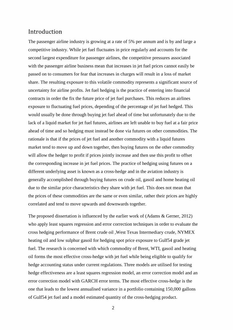
The passenger airline industry is growing at a rate of 5% per annum and is by and large a

competitive industry. While jet fuel fluctuates in price regularly and accounts for the

second largest expenditure for passenger airlines, the competitive pressures associated

with the passenger airline business mean that increases in jet fuel prices cannot easily be

passed on to consumers for fear that increases in charges will result in a loss of market

share. The resulting exposure to this volatile commodity represents a significant source of

uncertainty for airline profits. Jet fuel hedging is the practice of entering into financial

contracts in order the fix the future price of jet fuel purchases. This reduces an airlines

exposure to fluctuating fuel prices, depending of the percentage of jet fuel hedged. This

would usually be done through buying jet fuel ahead of time but unfortunately due to the

lack of a liquid market for jet fuel futures, airlines are left unable to buy fuel at a fair price

ahead of time and so hedging must instead be done via futures on other commodities. The

rationale is that if the prices of jet fuel and another commodity with a liquid futures

market tend to move up and down together, then buying futures on the other commodity

will allow the hedger to profit if prices jointly increase and then use this profit to offset

the corresponding increase in jet fuel prices. The practice of hedging using futures on a

different underlying asset is known as a cross-hedge and in the aviation industry is

generally accomplished through buying futures on crude oil, gasoil and home heating oil

due to the similar price characteristics they share with jet fuel. This does not mean that

the prices of these commodities are the same or even similar, rather their prices are highly

correlated and tend to move upwards and downwards together.

The proposed dissertation is influenced by the earlier work of (Adams & Gerner, 2012)

who apply least squares regression and error correction techniques in order to evaluate the

cross hedging performance of Brent crude oil ,West Texas Intermediary crude, NYMEX

heating oil and low sulphur gasoil for hedging spot price exposure to Gulf54 grade jet

fuel. The research is concerned with which commodity of Brent, WTI, gasoil and heating

oil forms the most effective cross-hedge with jet fuel while being eligible to qualify for

hedge accounting status under current regulations. Three models are utilised for testing

hedge effectiveness are a least squares regression model, an error correction model and an

error correction model with GARCH error terms. The most effective cross-hedge is the

one that leads to the lowest annualised variance in a portfolio containing 150,000 gallons

of Gulf54 jet fuel and a model estimated quantity of the cross-hedging product.

3

Jet Fuel Hedging

Jet fuel hedging is undertaken by a large number of airlines annually including Ryanair in

Europe and Southwest Airlines in the United States. Jet fuel is a volatile commodity and

from the early 2000’s the spot price of Gulf54 grade jet fuel rose from $0.53 per gallon to

over $4 per gallon at its peak in 2008, an increase of 647%. The price has since fallen

64% to $1.42 per gallon. Jet fuel accounts for the second largest expenditure for airlines

and since its price can drift substantially over time it’s found by (Carter, et al., 2006) that

if airlines can better manage the cost of fuel then they can more accurately estimate

budgetary costs and forecast future income. Fuel hedging also has positive benefits for the

overall value of the airline. Analysing US airlines over an eleven year period (Carter, et

al., 2006) find that participation in fuel hedging strategies is associated with increases in

airline value of between 5% and 10% while (Cobbs & Wolf, 2004) also determine that

using derivatives to hedge fuel costs creates a competitive advantage for the hedged

airline.

There are a number of strategies available to airlines when proposing hedging solutions to

the cost of jet fuel and (Cobbs & Wolf, 2004) suggest a strategy which is dynamically

managed throughout the life of the hedge achieves the greatest results and note that many

airlines prefer the use of over-the-counter derivatives such as collar structures and swaps

due to their customisability. Using these types of instruments airlines attempt to lock in

prices when they feel jet fuel prices are at a low point and cap prices when they feel they

are at a high point. While the use of these instruments represent a complex hedging

strategy (Carter, et al., 2004) note that their use has been quite successful for Southwest

Airlines. Not every airline will have the expertise to manage a derivative portfolio in

order to hedge fuel costs and so for other businesses hedging through the purchase of

commodity futures may be more appropriate.

Futures contracts allow one to enter into an agreement to buy a standardised quantity of

some product (say 1,000 gallons of Brent Crude Oil) for a certain price at a certain time in

the future. Unlike a Call Option which gives the buyer the right but not the obligation to

take delivery of the product, a futures contract is legally binding. As a result if an airline

enters into a futures contract to buy jet fuel at this time next year and the subsequent price

is below that which was agreed in the contract then the airline still has to pay the higher

price. From this perspective (Morrell & Swan, 2006) note that airlines hedge in order to

4

stabilize fuel prices, rather than speculate on whether the price of jet fuel will increase or

decrease in the future. A hedge is simply taking a position which minimises the price

variance of the asset being hedged. For example a $100 asset which is perfectly hedged

would never change in value from $100 regardless of market events. It’s also worth

noting that most futures are not settled with physical delivery of the underlying assets and

rather are settled for cash at maturity.

SFAS 133

Statements of Financial Accounting Standards 133 or SFAS 133 are an accounting

standard relating to ‘Accounting for Derivative Instruments and Hedging Activities’.

SFAS 133 was originally implemented as (FASB, 1998) which was introduced in order to

deal with some of the shortcomings of its predecessor SFAS 80. During the lifespan of a

derivatives hedge the value each derivative may deviate largely from its’ initial cost and

as a result the traditional accounting methods that required instruments to be booked and

carried at historical cost were not sufficient to reflect the true value of these derivative

assets whose prices changed daily. From this the first major doctrine of SFAS 133 is that

all derivative instruments are marked-to-market, or represented at their fair value. SFAS

133 also requires businesses to match gains in a derivative instrument with losses in a

hedged asset which has the effect of preventing companies from booking gains in either

the hedged item or derivative while failing to report losses on the other side of the hedge

until quarter close.

In order to qualify for hedge accounting under SFAS 133 it’s necessary for businesses to

demonstrate that each hedge is liable to be highly effective in reducing the risk exposure

of the underlying portfolio. It is noteworthy that (FASB, 1998) does not specify any one

measure of hedge effectiveness to be used in order to qualify for hedge accounting rules

and that the appropriateness of any assessment of hedge effectiveness can depend on the

nature of the risk being hedged. Once the measure of hedge effectiveness has been chosen

by the hedging party, (FASB, 1998) states that if the hedge fails this effectiveness test at

any time then the hedge ceases to qualify for hedge accounting rules. The (FASC, 2008)

note that the advantages of hedge accounting outweigh the disadvantages of fair value

accounting for financial instruments and there are a number of reasons why companies

want their hedge portfolios to qualify for hedge accounting rules. The principal advantage

is that it recognises the earnings effects of the hedging instrument and the hedged item in

5

the same financial period and also recognises their earnings effects in proportion to each

other which results in lower earnings volatility for companies. The lower earnings

volatility is in part due to the fact that when operating under hedge accounting rules

earnings and losses on hedged assets are deferred and recorded as offsetting gains or

losses in the value of the hedging instruments whereas outside these standards gains and

losses must be recorded individually and immediately (FASC, 2008).

In the absence of a specific recommendation much of the accounting profession has

adopted the 80-125 dollar offset ratio standard as a measure of hedge effectiveness. Under

current guidelines if one demonstrates that the R-Squared value obtained from regressing

price changes in the hedged asset on price changes in the hedging instrument is greater

than 0.8 then the hedge is deemed highly effective and will qualify for hedge accounting.

Hedge effectiveness is generally measured by the beta coefficient of a least squares

regression and must demonstrate that its value is greater than 0.8 at all times during the

life of the hedge in order to qualify for hedge accounting rules.

This method is criticised by (Charnes, et al., 2003) as during periods of low volatility the

R-Square value may fall below 0.8 and disqualify companies from hedge accounting and

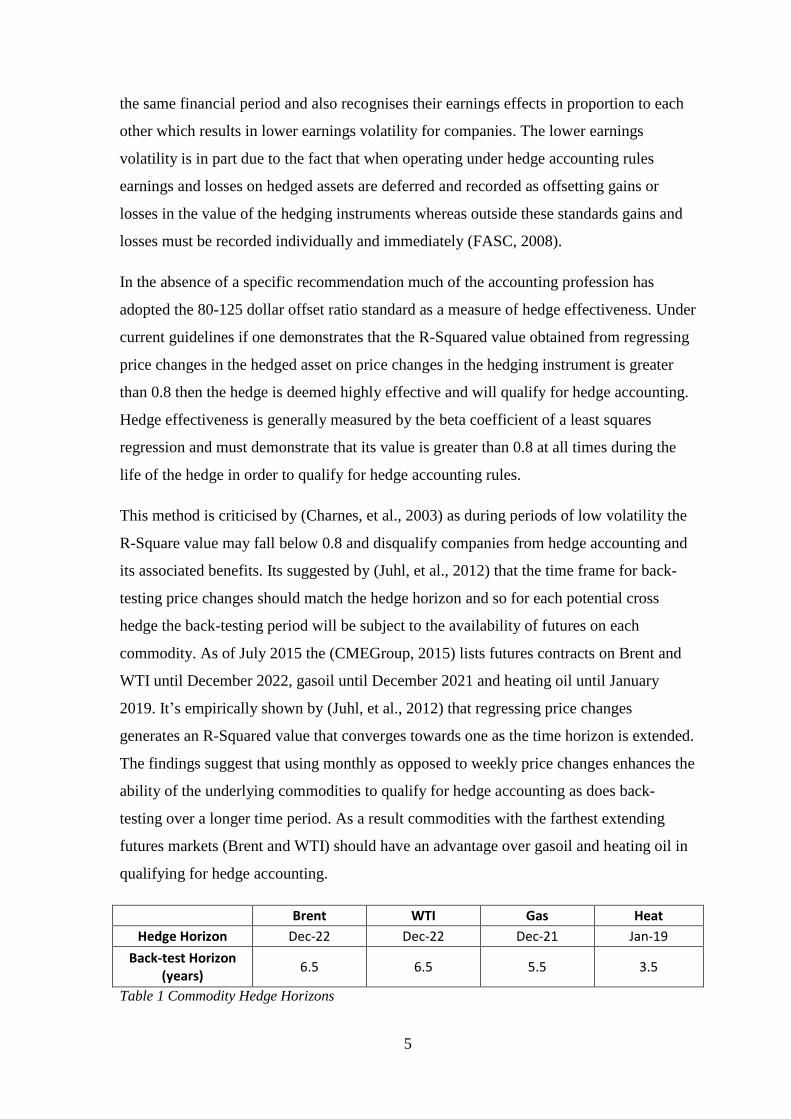
its associated benefits. Its suggested by (Juhl, et al., 2012) that the time frame for back-

testing price changes should match the hedge horizon and so for each potential cross

hedge the back-testing period will be subject to the availability of futures on each

commodity. As of July 2015 the (CMEGroup, 2015) lists futures contracts on Brent and

WTI until December 2022, gasoil until December 2021 and heating oil until January

2019. It’s empirically shown by (Juhl, et al., 2012) that regressing price changes

generates an R-Squared value that converges towards one as the time horizon is extended.

The findings suggest that using monthly as opposed to weekly price changes enhances the

ability of the underlying commodities to qualify for hedge accounting as does back-

testing over a longer time period. As a result commodities with the farthest extending

futures markets (Brent and WTI) should have an advantage over gasoil and heating oil in

qualifying for hedge accounting.

Brent WTI Gas Heat

Hedge Horizon Dec-22 Dec-22 Dec-21 Jan-19

Back-test Horizon (years)

6.5 6.5 5.5 3.5

Table 1 Commodity Hedge Horizons

6

(Juhl, et al., 2012) determine that if the commodity time series are co-integrated and that

price data is available for an adequate sample period then the hedger can be confident of

meeting hedge accounting standards and that with regards to hedge accounting it doesn’t

matter whether a least squares regression model or an error correction model are used to

determine hedge effectiveness as both will yield an R-Square that approaches one as the

hedge horizon is increased. In another study on optimal hedge ratio for cross-hedging jet

fuel (Adams & Gerner, 2012) perform hedge adjustments using a weekly horizon which

they note reduces commodity price risk without having to overspend on transaction fees

and is in line with other studies1. These studies do not account for the impact of hedge

accounting and while operating on a weekly horizon offers the opportunity to adjust the

hedge on a regular basis it may not display eligibility for hedge accounting under (FASB,

1998).

Starting with a weekly time horizon if the R-Square value lies below the 0.80 threshold

then the time horizon for the hedging product will be extended to monthly and re-

evaluated to see if the hedge meets SFAS accounting standards. The time horizon may

subsequently be extended up to a maximum of three months as each quarter is the

minimum time frame for which hedge effectiveness must be reported under FAS 133

guidelines. The time horizon for which each commodity qualifies for hedge accounting

(i.e. weekly, monthly or quarterly) will be the time frame carried forward for optimal

hedge ratio analysis. Due to the varying availability of futures contracts on Brent, WTI,

Gasoil and Home Heating oil and how this applies to (FASC, 2008), it will be assumed

that the hedge horizon for each commodity will be maximised in order to run the longest

possible back-test for each commodity. Thus the commodities Brent and WTI which have

the farthest extending futures will also have the longest back-test period.

1 (Clark, et al., 2003) (Coffey, et al., 2000)

7

Preliminary Considerations

Hedge Ratio & Hedging Performance

The hedge ratio is the proportion of the size of the position taken in futures contracts

compared to the size of the exposure. (Hull, 2015) notes that because jet fuel futures are

not actively traded airlines must hedge their exposure to jet fuel using futures on other

commodities in what is known as a cross-hedge. In a regular futures hedge when the asset

underlying the futures contract is the same as the asset being hedged the hedge ratio

would naturally be 1.0. Thus to hedge the cost of 10,000 barrels of crude oil the hedger

would have to buy 10 futures contracts, which corresponds to that exact amount. The goal

of hedging is to minimise the price variance of the hedged position. When the asset

underlying the futures contracts is not the same as the asset being hedged, their prices are

unlikely to be 100% correlated and so applying a hedge ratio of 1.0 may not be the best

solution.

Finding the hedge ratio which produces the minimum variance in the cross-hedge

portfolio is clearly dependent on the relationship between the price of the asset underlying

the futures contracts and the price of the asset being hedged. Studies such as (Ederington,

1979) were among the earliest to utilise the technique of regressing cash and futures

prices and use the resulting x-coefficient to determine the optimal cross-hedge ratio. This

has become the conventional approach in determining optimum hedge ratio though it has

been improved upon a number of times. In (Nelson & Plosser, 1982) it’s demonstrated

that non-stationary data (i.e. cash and futures price levels) can lead to inaccurate results in

regression testing. To account for these findings (Benninga, et al., 1984) introduce the

usage log returns in regression testing as they are trend stationary and this technique is

still widely used today. Through the regression method optimum hedge ratio is acquired

by finding the x-coefficient of an ordinary least squares (OLS) regression. (Hull, 2015)

describes the formula for optimal hedge ratio ℎ∗ as

ℎ∗ = 𝜌𝜎𝑆

𝜎𝐹

Equation 1 Optimal Hedge Ratio

In Equation 1 above 𝜎𝑆 corresponds to the standard deviation of the change in spot price,

𝜎𝐹 represents the standard deviation of the change in futures price and 𝜌 is the coefficient

of correlation between the spot and the futures prices. It’s maintained within the SFAS

133 regulations that the back-tested for a period for testing hedge effectiveness should be

8

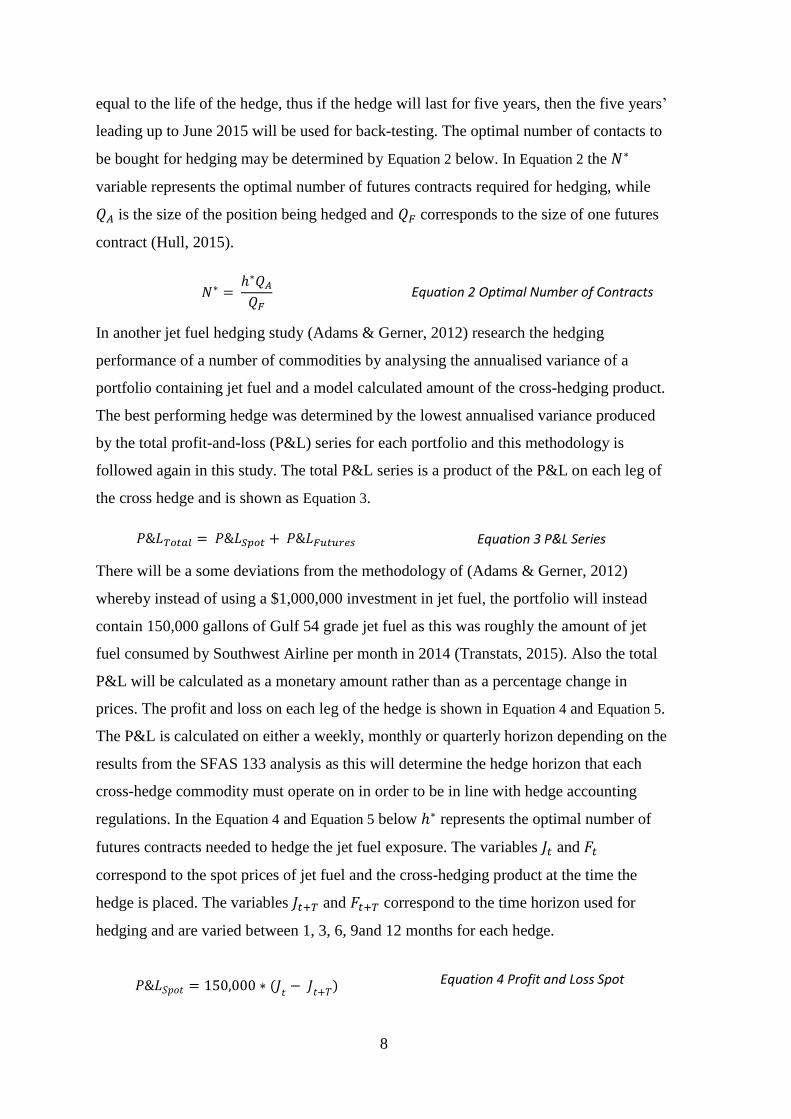
equal to the life of the hedge, thus if the hedge will last for five years, then the five years’

leading up to June 2015 will be used for back-testing. The optimal number of contacts to

be bought for hedging may be determined by Equation 2 below. In Equation 2 the 𝑁∗

variable represents the optimal number of futures contracts required for hedging, while

𝑄𝐴 is the size of the position being hedged and 𝑄𝐹 corresponds to the size of one futures

contract (Hull, 2015).

𝑁∗ = ℎ∗𝑄𝐴

𝑄𝐹 Equation 2 Optimal Number of Contracts

In another jet fuel hedging study (Adams & Gerner, 2012) research the hedging

performance of a number of commodities by analysing the annualised variance of a

portfolio containing jet fuel and a model calculated amount of the cross-hedging product.

The best performing hedge was determined by the lowest annualised variance produced

by the total profit-and-loss (P&L) series for each portfolio and this methodology is

followed again in this study. The total P&L series is a product of the P&L on each leg of

the cross hedge and is shown as Equation 3.

𝑃&𝐿𝑇𝑜𝑡𝑎𝑙 = 𝑃&𝐿𝑆𝑝𝑜𝑡 + 𝑃&𝐿𝐹𝑢𝑡𝑢𝑟𝑒𝑠 Equation 3 P&L Series

There will be a some deviations from the methodology of (Adams & Gerner, 2012)

whereby instead of using a $1,000,000 investment in jet fuel, the portfolio will instead

contain 150,000 gallons of Gulf 54 grade jet fuel as this was roughly the amount of jet

fuel consumed by Southwest Airline per month in 2014 (Transtats, 2015). Also the total

P&L will be calculated as a monetary amount rather than as a percentage change in

prices. The profit and loss on each leg of the hedge is shown in Equation 4 and Equation 5.

The P&L is calculated on either a weekly, monthly or quarterly horizon depending on the

results from the SFAS 133 analysis as this will determine the hedge horizon that each

cross-hedge commodity must operate on in order to be in line with hedge accounting

regulations. In the Equation 4 and Equation 5 below ℎ∗ represents the optimal number of

futures contracts needed to hedge the jet fuel exposure. The variables 𝐽𝑡 and 𝐹𝑡

correspond to the spot prices of jet fuel and the cross-hedging product at the time the

hedge is placed. The variables 𝐽𝑡+𝑇 and 𝐹𝑡+𝑇 correspond to the time horizon used for

hedging and are varied between 1, 3, 6, 9and 12 months for each hedge.

𝑃&𝐿𝑆𝑝𝑜𝑡 = 150,000 ∗ (𝐽𝑡

− 𝐽𝑡+𝑇) Equation 4 Profit and Loss Spot

9

𝑃&𝐿𝐹𝑢𝑡𝑢𝑟𝑒𝑠 = (𝐹𝑡+𝑇

− 𝐹𝑡) ∗ℎ∗ ∗ 150,000

𝑄𝐹

Equation 5 Profit and Loss Futures

The total returns series is a sum of Equation 4 and Equation 5 for each time period during

the back-testing window. The best performing cross-hedge will be the one which

produces the lowest annualised variance as measured by the standard deviation of the

total profit and loss series multiplied by the square root of number of periods per year.

For example the annualised variance equation for gasoil being hedged on a monthly

horizon is given in Equation 6, and the annualised variance will be calculated for each of

the three models across all time horizons.

𝐴𝑛𝑛 𝑉𝑎𝑟 = 𝑠𝑡𝑑(𝑇𝑜𝑡𝑎𝑙 𝑃&𝐿𝐺𝑎𝑠𝑜𝑖𝑙) ∗ √12 Equation 6 Annualised Variance Gasoil

The methodology for determining the optimal hedge ratio also differs from that of

(Adams & Gerner, 2012) in that the price levels are transformed to first differences

instead of log returns before being input into the OLS, ECM and ECM-GARCH models.

The reason for this approach is due to the way the P&L is calculated. Determining

optimal hedge ratio using log returns would yield erroneous P&L results as using log

returns does not capture the magnitude of the changes in monetary value for each

commodity, i.e. a positive 1% return of Gasoil does not perfectly hedge a 1% loss on jet

fuel because their prices are vastly different and this must be captured in the P&L

calculation. The final P&L methodology change from (Adams & Gerner, 2012) in how

the dynamic cross hedge ratio is calculated. In the analysis instead of calculating a new

optimal cross hedge ratio for each year based on all the previously available data, the 𝛽

value is calculated for each hedge placed during back-testing based on the most recent 5,

10 and 15 years of data to contrast the differences (if any) resulting from including more

years of data in determining optimal hedge ratio.

Hypothesis Testing & Statistical Significance

The methodology utilises a number of hypotheses tests throughout. Hypotheses are

investigated by specifying a null hypothesis and investigating whether this condition can

be accepted or rejected based on the evidence presented. In hypothesis testing the null

hypothesis is presumed to be true, until the data presented provides sufficient evidence to

show that it is not. There are two outcomes to hypothesis testing, rejecting the null and

failing to reject the null. The terminology here is important, as the null can never truly be

10

accepted, only rejected or not rejected based on the sample provided. Think in terms of a

murder trial where the null hypothesis is that the accused is innocent. There are two

outcomes, the first is that the court may be provided with sufficient evidence to reject this

hypothesis, i.e. the accused is guilty. On the other hand the trial may be provided be

insufficient evidence to reject this hypothesis. This doesn’t mean that the null hypothesis

is true and that the accused is innocent, just that there is not sufficient evidence to

disprove the null and the trial has found them not guilty i.e. it has failed to reject the null.

When carrying out a hypothesis test one must specify a significance level which also

represents the ‘size’ of the test. The test ‘size’ is the probability of falsely rejecting the

null i.e. the probability of a type I error (Alexander, 2008). A type I error is the false

rejection of a true null hypothesis, i.e. detecting an affect that is not present. There is also

a type II error which is failing to reject a false null hypothesis, i.e. failing to detect and

affect that is present. Thought of another way a type I error is finding an innocent person

guilty while a type II error is finding a guilty person innocent, and when testing a type I

error is more serious. Increasing the significance level reduces the size of the test but also

increases the probability of a type II error, thus decreasing its’ power which is a tests

ability to correctly reject the null hypothesis (Alexander, 2008).

The critical values for each hypothesis test represent the upper and lower percentiles of

the sample. Thus if the significance level is 5%, the critical values represent the points

between which 95% of the data lies. As a result choosing a lower significance level (of

say 90%) increases the tests chance of rejecting the null hypothesis but suffers from

losing statistical power making the results less convincing (Banerjee, et al., 1993). For the

null hypothesis to be rejected the test statistic must fall within the critical region (be more

extreme than the critical values) and produce a pValue which is lower than the

significance level. For a one sided hypothesis test such as the (Dickey & Fuller, 1979) test

for a unit root the test statistic must fall below the critical value.

11

Regression Model

A theoretical framework for determining the optimal futures position in a cross hedge is

described in (Anderson & Danthine, 1981) who specify that the proportion of output that

should be hedged in each contract, i.e. the cross-hedge ratio, is determined by the slope

coefficient output from regressing cash prices on futures prices. For most practical

purposes (Conroy, 2003) notes that one can simply use the spot prices for the cross-hedge

commodities in determining optimal hedge ratio and so that is the method pursued in this

paper. For practical purposes however the cross-hedge product spot prices will still be

referred to as futures prices for distinction from the jet fuel spot prices. The price levels

for each commodity represent a non-stationary array of data. The research of (Nelson &

Plosser, 1982) demonstrated that non-stationary data can lead to inaccurate results in

regression testing, and so to account for these findings (Benninga, et al., 1983) introduce

the usage log returns in place of cash and futures prices and this method is found to lead

to more accurate results when using regression methods for commodity hedging (Myers

& Thompson, 1989).

The use of regression testing also provides a measure of explanatory power between the

dependent and independent variables. The R-Squared value indicates the percentage of

variation in jet fuel returns which can be explained by the variation in the returns of the

cross-hedging products. While regression analysis has the advantage of being straight

forward to implement (Cecchetti, et al., 1988) note that this process for estimating

optimal hedge ratio suffers from major drawbacks. This research cites that no adjustment

can be made for the fact that the joint distribution of the time series varies over time and

that this important characteristic cannot be captured via the OLS approach. Other issues

are noted by (Kroner & Sultan, 1993) who show that if the time series are co-integrated

that the regression is misspecified as it involves over differencing the data and losing

information regarding the long run relationship between the spot and futures prices. This

can lead to a downward bias in hedge ratio estimation and as a result under-hedging.

Unit Root Testing

In time series analysis a trend-stationary series is one whose error term follows a

stationary process while an integrated time series is one whose error term follows a

random walk (DeJong, et al., 1992). Tests for stationarity are carried out on each of the

12

series as (Granger & Newbold, 1974) show that two integrated time series which are

completely unrelated can demonstrate an apparently significant relationship when one is

regressed on the other. The findings of (Granger & Newbold, 1974) led econometric

analysis to become interested in transformations to induce stationarity. Stationary series

have a number of favourable characteristics such as a finite variance and finite time

between crossings of the series mean, as well as this stationary series have the important

property that certain functions of the sample values converge to constants as the number

of sample values increases (Banerjee, et al., 1993). This means that for stationary time

series the mean and variance of the sample being tested converge towards the true mean

and variance of the process as the sample size is increased.

Shown below in Table 2 are the hypotheses for a unit root test where the variables display

either a stationary I(0) or a non-stationary I(1) trend. Its’ noted by (Alexander, 2008) that

if the test statistic falls outside the critical region and the null hypothesis is not rejected

that another unit root test should be performed of the first differenced time series to

analyse its order of integration. Differencing involves calculating the differences between

consecutive observations in a time series. The first difference of a time series 𝑥 at period 𝑡

is 𝑥𝑡 − 𝑥𝑡−1. If the price levels for any of the commodities analysed are found to be non-

stationary and 𝑦𝑡, the first differenced time series of that commodity, is subsequently

found to be stationary then the time series being analysed is termed to be integrated of the

order I(1). If the sample does not achieve stationarity until its second differences (the first

difference of 𝑦𝑡) then the sample is said to be integrated of the order I(2). Thus unit root

testing is not only useful in identifying stationary trends in data but also helps to identify

the order of integration of each time series.

Levels 𝐻0: 𝑋𝑡 ~ 𝐼(1) 𝐻1: 𝑋𝑡 ~ 𝐼(0)

First Differences 𝐻0: ∆𝑋𝑡 ~ 𝐼(1) 𝐻1: ∆𝑋𝑡 ~ 𝐼(0)

Table 2 Unit Root Hypotheses

As part of the methodology the Augmented Dickey-Fuller (ADF) test of (Dickey &

Fuller, 1979) will be carried out on the data to test each time series for stationarity. An

ADF test is a unit root test which returns a rejection decision based on the detection of a

unit root in the time series. The null hypothesis is that a unit root exists and the time

series is integrated, thus a rejection of the null hypothesis indicates that the time series is

trend-stationary. It is noted by (Alexander, 2008) that the ADF test is also the least

13

powerful unit root test. This is likely because the impact of type I errors have on the

results, i.e. at a 5% significance level the ADF test will incorrectly return a decision of

stationarity (where none is present) approximately once every twenty times. To account

for this the KPSS test of (Kwiatkowski, et al., 1992) will also be carried out on each time

series. The KPSS test is a stationarity test in which the null hypothesis is that the time

series is trend-stationary and it is expected the KPSS results should be consistent with the

ADF tests.

Regression Analysis

Regression testing is a process which involves evaluating the linear relationship between

variables. Regression analysis typically indicates how the value of a dependent variable

changes as a result of changes in value of some independent variable. Using this

statistical method we wish to find out how a change in the value of 𝑋 affects the value

of 𝑌, or looked at in a slightly different way, can we use the observed change in the value

of 𝑋 to predict the resulting change in the value of 𝑌. The simplest example of a linear

relationship is given by the equation of a straight line in Equation 7.

𝑌𝑡 = 𝛼 + 𝛽𝑋𝑡 + 휀𝑡 Equation 7 Linear Model

In Equation 7 above 𝑌 represents the dependent variable (jet fuel spot) and 𝑋 represents

the independent variable (commodity futures) while the intercept and slope of the

regressions line of best fit between the two are denoted by 𝛼 and 𝛽 respectively. The x-

coefficient or 𝛽 value also corresponds to the optimal hedge ratio estimated by the linear

regression. Figure 1 illustrates a regression between the first differenced series for Brent

crude oil and Gulf54 grade jet fuel. From Figure 1 it’s clear that not all of the data points

will form a perfectly straight line and as a result an error term is included in Equation 7

Linear Model which defines the distance between each data point and the regression line of

best fit. If the correlation between 𝑋 and 𝑌 is low then one would observe a high variance

in the errors which are represented in Equation 7 by 휀𝑡 while a high correlation between

regression variables would yield a low variance in 휀𝑡 (Alexander, 2008).

14

Figure 1 Jet-Brent OLS Regression Plot

Ordinary least squares (OLS) is a technique for estimating the unknown parameters of a

linear regression by minimising the regression residuals. The residuals represent the

difference between the observed value and the estimated value of the quantity of interest.

In the context of cross hedging where one is attempting to understand how changes in the

price of futures contracts can predict changes in the spot price of jet fuel, the OLS

regression will attempt to fit a linear model to the data such that the errors between the

predicted change in jet fuel spot prices and actual observed changes are minimised. The

research of (Engle & Granger, 1987) among others notes that the residual series made up of the

error terms may retain important information about the relationship between the variables.

Characteristics such as its speed of adjustment towards the line of best fit and whether the error

terms are autocorrelated remain unaccounted for in the linear regression model (Kroner & Sultan,

1993).

While regression analysis is unable to capture several time series characteristics important

in determining optimum hedge ratio the technique has been shown in some scenarios to

outperform other models such as the error correction model that captures long a short run

hedge dynamics. Using futures on the Nordic power exchange (Byström, 2003)

determines that an OLS hedge outperforms more elaborate moving average and

generalized autoregressive conditional heteroscedasticity (GARCH) hedging models. In

further support of OLS hedging methods (Lien, et al., 2002) find the OLS technique

outperforms a (vector) VGARCH model when hedging a sample of currency, commodity

15

and stock index futures. This may be related to the findings of (Stock, 1987) that if time

series are co-integrated and the 𝛼′𝑦𝑡 combination of its co-integrating vector and

logarithm vector is I(0) then a simple regression is likely to yield very consistent results

of the co-integrating vector (Baille & Bollerslev, 1994). In contrast with these findings

(Ghosh, 1993) shows that an error correction model (ECM) presents a significant

improvement over the OLS regression approach when determining optimum hedge ratios

using stock index futures as this method incorporates non-stationarity, the long run

equilibrium relationship and short-run dynamics of each time series. Similarly (Chou, et

al., 1997) find an ECM outperforms the traditional regression approach when Japans

Nikkei Stock Average index futures.

Residual Series

There are some characteristics of the residual time series resulting from the OLS

regression approach which can provide important information surrounding the suitability

of each model to fit the data. Autocorrelation refers to the cross-correlation of a signal

with itself at different points in time while heteroscedasticity refers to the mean variance

in the residual series changing over time (Engle, 1982). The influence of

heteroscedasticity and autocorrelation in the error structure (residuals) of a regression

may lead to spurious results if not accounted for in the analysis (Granger & Newbold,

1974).

In large sample sizes (Alexander, 2008) notes that the presence of autocorrelation and

heteroscedasticity will not have a damaging impact on the outcome of an OLS regression

but that in a small sample size where autocorrelation and heteroscedasticity are detected a

generalised least squares approach should be used instead of the ordinary least squares

method. This has consequences surrounding the hedge horizon used for testing as if hedge

horizon is increased past a monthly basis in order to meet hedge accounting standards, it

will greatly reduce the amount of data available for testing which could potentially

increase the impact that autocorrelation and heteroscedasticity can have on the results.

Autocorrelation

Autocorrelation is the linear dependence of a variable with itself at two different points in

time, or looked at in another way an autocorrelated time series is one which exhibits

similarity with a lagged version of itself. A basic assumption underlying the OLS

16

regression is that the error terms are independent and once this assumption is satisfied the

OLS procedure is valid whether or not the time series themselves are serially correlated

(Durbin & Watson, 1950). From this we can deduce that it is not important to test the

individual commodity time series for autocorrelation but instead need to analyse the

residual series produced by each OLS regression. The presence of autocorrelation is a

problem in the least squares approach because it indicates that the error terms are not

independent and this may lead to the variance of the least square estimators in the

regressions to be too large (Anderson, 1954). The presence of autocorrelation may require

modification to the usual methods of estimation and prediction and (Cochrane & Orcutt,

1949) note that when estimates of autoregressive properties are based on autocorrelated

residuals there is a large bias towards randomness. This implies that the presence of

autocorrelation in the residual series may substantially impact the results derived from the

ECM and ECM-GARCH models which incorporate residual information, or rather it can

diminish the advantage the ECM and ECM GARCH models have over the OLS

regression because the presence of autocorrelation muddles the useful information

contained in the residuals.

Heteroscedasticity

Heteroscedasticity refers to sub-populations in a collection of random variables having

different variability’s from others, which translates to the time series demonstrating

different variances over time. In a residual series this translates to serially uncorrelated

residual errors displaying a constant unconditional variance but a non-constant

conditional variance (Engle, 1982). Before the autoregressive conditional

heteroscedasticity (ARCH) model proposed by (Engle, 1982) most econometric models

assumed constant variance. The defining feature of an autoregressive conditional

heteroscedastic (ARCH) process is the specification of a non-constant variance which is

conditional on past variance levels. Under ARCH the conditional variance of the current

error term is dependent on its’ realised past values and (Engle, 1982) notes this model has

the advantage of reflecting clustering between large and small error terms (i.e. volatility

clustering).Thus in an ARCH process periods of low volatility tend to be followed by

periods of low volatility while periods of high volatility tend to be followed by further

periods of high volatility.

17

Error Correction Model

The error correction model (ECM) represents an extension of the OLS regression and

operates on the premise that important information that predicts the future evolution of

the time series under analysis is retained in the residual time series. As a result the ECM

incorporates a lagged version of the residual errors in order to capture elements of the

short term relationship between the variables. The ECM also accounts for the long run

equilibrium relationship between the time series through considering the presence of a co-

integration relationship between the variables. The research of (Engle & Granger, 1987)

shows that if the linear combination of two non-stationary variables forms a stationary

time series, then the equilibrium condition and adjustment process to equilibrium can be

represented by an error correction model (Ghosh, 1993). The incorporation of elements

that capture some of the short and long run dynamics of the time series accounts for a

number of the disadvantages of the OLS regression noted by (Kroner & Sultan, 1993).

Co-Integration

Integrated time series are non-stationary and tend to drift randomly over time, yet some

pairs of integrated series may be defined by some long-run relationship to which the

system converges to over time (Banerjee, et al., 1993). The research of (Engle & Granger,

1987) makes note that economic time series can wander substantially and yet some series

are expected to move so that they do not drift too far apart. If two time series are co-

integrated it will be observed that over time they will tend not to drift too far apart and

that the distance between them (i.e. their residual series) will follow a stationary trend that

is normally distributed around some mean value. The presence of co-integration suggests

a long run memory between the co-integrated time series. While the series may diverge

substantially in the short run and the effects of shocks may only vanish over long time

horizons, pairs of co-integrated series will always display a tendency over time to drift

back towards their equilibrium relationship (Baille & Bollerslev, 1994). In this respect the

drift between co-integrated series must be stochastically bounded and, at some point,

diminishing over time (Banerjee, et al., 1993). In terms of the time series which represent

jet fuel and each of the cross-hedge commodity prices, carrying out tests for co-

integration will indicate whether or not their price series are linked in the long run and

forms the basis of fitting an error correction model to the data (Stock & Watson, 1988).

18

“The components of the vector 𝑥𝑡 are said to co-integrated of order 𝑑, 𝑏, denoted

𝑥𝑡 ~ 𝐶𝐼(𝑑, 𝑏), if (i) all components of 𝑥𝑡 are I(d); (ii) there exists a vector α (≠0) so that

𝑧𝑡 = 𝛼′𝑥𝑡 ~ 𝐼(𝑑 − 𝑏), b > 0. The vector α is called the co-integrating vector”

To make sense of the co-integration definition above offered by (Engle & Granger, 1987)

consider the components of the vector 𝑥𝑡 are two time series 𝑗𝑡 and 𝑓𝑡 which represent the

spot price of jet fuel and the futures price of the cross-hedging commodity. Assume the

unit root tests carried out determine that 𝑗𝑡 and 𝑓𝑡 are both I(1) integrated variables which

fulfils the first condition in the above definition. It is noted by (Engle & Granger, 1987)

that for most observations 𝛼′𝑥𝑡 will not be in equilibrium and that there exists a univariate

quantity outlined above as 𝑧𝑡 called the equilibrium error. If there exists some vector α

such that the residual error series 𝑧𝑡 formed by a linear combination of α with 𝑥𝑡 is I(0),

or trend-stationary, then the second condition is fulfilled and time series 𝑗𝑡 and 𝑓𝑡 are said

to be co-integrated.

In other words co-integration implies that deviations from equilibrium are stationary with

finite variance even though the series themselves may be non-stationary with infinite

variance. Thus if 𝑧𝑡 represents the error or distance from 𝛼′𝑥𝑡 to the long run equilibrium,

it can be used to independently verify the existence of co-integration between time series

𝑗𝑡 and 𝑓𝑡 by testing whether the residuals derived from a regressing 𝑗𝑡 on 𝑓𝑡 display

stationarity.

It’s shown by (Ghosh, 1993) that smaller than optimal futures positions are taken when

the effect of co-integration is omitted from hedging models. A number of fuel hedging

strategies are described by (Cobbs & Wolf, 2004) however they fail to acknowledge a co-

integration relationship between the jet fuel and any of the cross-hedging products as

being significant though its importance is recognised in the research by (Adams &

Gerner, 2012) on which this study is based. It’s inclusion in the analysis is deemed

essential as “co-integration is the only true indispensable component when comparing ex-

post performance of various hedge strategies” (Da-Hsiang, 1996). There are a number of

tests for co-integration which may be pursued in this study, however the simple two-step

estimation of (Engle & Granger, 1987) is followed for a number of reasons. The two-step

estimation has a very practical advantage of being the most straight-forward of co-

integration tests and is easily implemented in MATLAB. Alternative cointegration testing

methods are available such as the vector auto-regression (VAR) method of (Johansen,

19

1991) which allows for testing of co-integration rank and seasonal dummies among the

variables. However due to each potential co-integration relationship containing only a

pair of variables, the more complex approach associated with the VAR method of

(Johansen, 1991) is rejected in favour of the more straight forward two-step approach of

(Engle & Granger, 1987). The effect of co-integration when hedging jet fuel futures is

studied by (Adams & Gerner, 2012) who’s research found that an error correction model

(ECM) outperforms an OLS regression when cross-hedging jet fuel with a number of

crude oil based commodities.

Error Correction Analysis

Error correction terms may be used as a way of capturing adjustments in a dependent

variable which depended not on the corresponding level of some explanatory variable but

on the extent to which the explanatory variable deviated from its equilibrium relationship

with the dependent variable (Banerjee, et al., 1993). In other words, assuming that some

long run equilibrium relationship is present between the time series (which is why co-

integration is a prerequisite), an error correction model (ECM) may be used to estimate

adjustments in jet fuel prices based on how its time series has deviated from its’

equilibrium relationship with the cross-hedging product. It’s noted by (Engle & Granger,

1987) that for a two variable system a classic error correction model would relate the

changes in one variable to past equilibrium errors as well as past changes in both

variables. (Kroner & Sultan, 1993) note that regression models can obscure the long run

relationship between spot and futures prices while (Adams & Gerner, 2012) note that the

ECM framework accounts for the autoregressive structure of spot and forward price

changes and thus incorporates the long run relationship between both markets. It can be

viewed such that if an OLS regression estimates the linear relationship between the first

differences for jet fuel and the hedging commodity, then the error correction model estimates the

dynamic structure between the first differenced series by incorporating short and long run

information about their co-integrated relationship (Alexander, 2008). The model operates on the

idea that the short term deviations from the long run equilibrium relationship will be subsequently

corrected by the time series on its own.

The error correction model employed in the methodology is the same one employed by

(Adams & Gerner, 2012) with the substitution of first differences for log returns and takes

the form

20

∆𝑓𝑑𝑆𝑡 = 𝑐 + 𝛽∆𝑓𝑑𝐹𝑡,𝑇 + ∑ 𝛾𝑘∆𝑓𝑑𝐹𝑡−𝑘,𝐾

𝐾

𝑘=1

+ ∑ 𝛿𝑙∆𝑓𝑑𝑆𝑡−𝑙

𝐿

𝑙=1

+ 𝜆𝑒𝑡−1 + 휀𝑡

Equation 8 Error Correction

Model

Where ∆𝑓𝑑𝑆𝑡 and ∆𝑓𝑑𝐹𝑡,𝑇 represent the changes in the first differenced price series, 𝑐 represents

the intercept and 𝛾𝑘 and 𝛿𝑙 signify the short run dynamics coming from the lagged changes in the

spot price (hence 𝐹𝑡−𝑘,𝐾). The 𝜆 term represents the adjustment parameter which captures the

speed at which each time series reacts to deviations from the long run equilibrium relationship

and 𝑒𝑡 is the error term, which comes in lagged form, as each time series must first deviate from

the long run relationship before beginning its correction process. The 𝑒𝑡 term is formed by the

residual series from an OLS regression of the differenced series for jet fuel on the differenced

series for the chosen cross-hedge commodity. Finally 휀𝑡 represents the standard error while 𝛽

represents the optimal hedge ratio.

The ECM analysis will be carried out using the same rolling window as the OLS regression and

will convert the residual series produced by each loop of the OLS regression model to lagged

form for use in the ECM, as shown in the MATLAB Dynamic Hedge Ratio section of

Appendix B. Like the OLS model the ECM will be run on either a weekly, monthly or quarterly

hedging horizon based on the SFAS 133 analysis for each commodity. The model itself is based

on data provided by (Adams, 2015). Since it’s noted by (Kroner & Sultan, 1993) that an OLS can

result in downward bias which leads to under hedging we may observe a slightly higher optimal

hedge ratio output from the error correction model when compared to the ordinary least squares

regression model.

The representation theorem of (Granger, 1986) specifies that that when integrated

variables share a co-integration relationship that a vector autoregressive (VAR) model of

first differences will be misspecified as the disequilibrium term is missing from the vector

autoregressive representation. This term is also missing from the more simplified OLS

regression Equation 7 outlined above. It’s noted by (Alexander, 2008) that when lagged

disequilibrium terms are included as explanatory variables that the model becomes well

specified. As shown above in Equation 8 the error correction framework accounts for the

misspecification of OLS regression models and VAR models by including a lagged error

correction term in order to incorporate the previous periods’ equilibrium error (Ghosh,

1993). The model also includes additional information about the lagged series through a

linear combination of the lagged values of the first differenced time series for each

commodity with a term that estimates the short run dynamics.

21

GARCH Extension

The OLS regression has been described by (Engle, 2001) as the “great workhorse of

applied econometrics” however he notes that when attempting to estimate and examine

the size of the errors within a model that the questions are about volatility, for which the

standard tools are the ARCH and GARCH models. Generalised autoregressive

conditional heteroscedasticity (GARCH) is a generalisation of the ARCH process

discussed earlier whereby the variance of the error terms is assumed to follow an

autoregressive moving average (ARMA) process. GARCH models are thus an extension

of the non-constant conditional variance approach of ARCH models whereby the

conditional variance at any one time is based on a weighted sum of its passed values. The

GARCH model of (Bollerslev, 1986) is generally considered superior because it can

account for the time varying variance of the spot and futures prices during the life of the

hedge and can also account for price shocks. While the classic error correction model

incorporates the cointegrated relationship and lagged residuals in order to capture the

short and long run dynamics between the time series, the GARCH extension substitutes

the lagged residual series for GARCH residuals in order to capture the non-constant

conditional variance of the residual time series as well as the short run dynamics.

GARCH Analysis

The error correction model employed by (Adams & Gerner, 2012) also specifies a

GARCH extension to obtain greater accuracy and they state that a univariate GARCH

should be sufficient to model the optimal hedge ratio. In contrast studies such as (Kroner

& Sultan, 1993) and (Baillie & Myers, 1991) use a bivariate GARCH model as they state

that in the case of two I(1) variables being co-integrated so that their linear combination is

I(0) then they should be represented by a bivariate model that includes an error correction

term. For the purpose of simplicity a univariate GARCH approach is taken where the

non-constant conditional variance is estimated using Equation 9. In order to incorporate

GARCH residuals into the model the lagged residual series used in the regular ECM will

be transformed to its GARCH representation using Equation 9 and then analysed in the

same way as the regular ECM.

ℎ𝑡2 = 𝜇 + 𝜃1휀𝑡−1

2 + 𝜃2ℎ𝑡−12 Equation 9 Conditional Variance

22

In a study based on exchange rates (Hansen & Lunde, 2005) find that there is no evidence

to suggest that a GARCH(1,1) model is outperformed by over 330 other ARCH-type

models in its ability to model conditional variance. Dynamic hedging using an error

correction model with a GARCH error structure was carried out by (Kroner & Sultan,

1993) using a GARCH(1,1) model while (Adams & Gerner, 2012) also employ the this

type of model for capturing non-constant condition variance. For these reasons a

GARCH(1,1) will be fitted to the data in order to compute the GARCH residuals. In a

GARCH(1,1) model the conditional variance is based on the most recent observation of

the residuals and the most recent estimate of the variance rate as shown by the 𝑡 − 1

subscript for the variables in Equation 9. The GARCH model will be fitted using the

MATLAB ‘estimate’ function which estimates the GARCH(1,1) model via maximum

likelihood methods. As with the lagged residuals of the ECM the ECM-GARCH will be

based off a new set of OLS residuals generated with every loop of the model. Once the

GARCH model has been fitted using the MATLAB function the residuals will be

transformed using Equation 9. Each residual may be represented as √ℎ𝑡2 and will be

substituted for the lagged error terms in the ECM model.

Basis Risk

Basis risk is described by (Figlewski, 1984) as the varying nature of the difference

between the spot and futures prices and that hedging using futures exposes the position to

this type of risk since the evolution of the futures price over time may not match the

change in value of the cash position. Since this basis may be represented by the residual

series between the spot and futures prices, then the error correction models incorporation

of the lagged error term as well as the adjustment parameter should enable an ECM to

better account for the evolution of basis risk when compared to an OLS regression. It’s

observed by (Figlewski, 1984) that this type of risk increases as the length of the hedging

horizon decreases so it’s likely that if the hedge horizon must be increased in order to

meet hedge accounting standards as per (Juhl, et al., 2012) that this will have the effect of

reducing basis risk for all of the models analysed.

23

Results & Discussion

SFAS 133

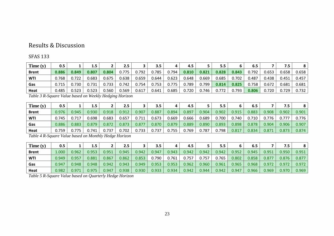
Time (y) 0.5 1 1.5 2 2.5 3 3.5 4 4.5 5 5.5 6 6.5 7 7.5 8

Brent 0.886 0.849 0.807 0.804 0.775 0.792 0.785 0.794 0.810 0.821 0.828 0.843 0.792 0.653 0.658 0.658

WTI 0.768 0.722 0.683 0.675 0.638 0.659 0.644 0.623 0.648 0.669 0.685 0.702 0.487 0.438 0.451 0.457

Gas 0.715 0.730 0.731 0.733 0.742 0.754 0.753 0.775 0.789 0.799 0.814 0.825 0.758 0.672 0.681 0.681

Heat 0.485 0.523 0.523 0.560 0.569 0.617 0.641 0.685 0.720 0.746 0.772 0.793 0.806 0.720 0.729 0.732 Table 3 R-Square Value based on Weekly Hedging Horizon

Time (y) 0.5 1 1.5 2 2.5 3 3.5 4 4.5 5 5.5 6 6.5 7 7.5 8

Brent 0.976 0.945 0.930 0.918 0.912 0.907 0.887 0.894 0.897 0.904 0.902 0.915 0.883 0.908 0.902 0.901

WTI 0.745 0.717 0.698 0.683 0.657 0.711 0.673 0.669 0.666 0.689 0.700 0.740 0.710 0.776 0.777 0.776

Gas 0.886 0.883 0.879 0.872 0.873 0.877 0.870 0.879 0.889 0.890 0.893 0.898 0.878 0.904 0.906 0.907

Heat 0.759 0.775 0.741 0.737 0.702 0.733 0.737 0.755 0.769 0.787 0.798 0.817 0.834 0.871 0.873 0.874 Table 4 R-Square Value based on Monthly Hedge Horizon

Time (y) 0.5 1 1.5 2 2.5 3 3.5 4 4.5 5 5.5 6 6.5 7 7.5 8

Brent 1.000 0.962 0.953 0.951 0.945 0.942 0.947 0.943 0.942 0.942 0.942 0.952 0.945 0.951 0.950 0.951

WTI 0.949 0.957 0.881 0.867 0.862 0.853 0.790 0.761 0.757 0.757 0.765 0.802 0.858 0.877 0.876 0.877

Gas 0.947 0.948 0.948 0.942 0.943 0.949 0.953 0.953 0.962 0.960 0.961 0.965 0.968 0.972 0.972 0.972

Heat 0.982 0.971 0.975 0.947 0.938 0.930 0.933 0.934 0.942 0.944 0.942 0.947 0.966 0.969 0.970 0.969 Table 5 R-Square Value based on Quarterly Hedge Horizon

24

Table 3, Table 4 and Table 5 on the previous page present the results of simple regression

analysis on the log returns series for jet fuel on the log returns series for each of cross-hedge

commodities. The R-Square values of each regression are presented as these values may be

presented as a means to qualify for hedge accounting status. It is recommended by (FASC,

2008) that the back-testing period for each commodity matches the hedge horizon and so the

times in years across the top of each of the tables correspond to horizons extending

backwards from June 1st 2015. Thus the results presented as 0.5 years correspond to an R-

Square derived from using data from January 1st 2015 to June 1

st 2015, 3 year results

correspond to testing from June 1st 2012 to June 1

st 2015 etc. The threshold for qualifying for

hedge accounting is an R-Square value of 0.8 and in Table 3, Table 4 and Table 5 the R-Square

results which meet this criteria are highlighted in green. Each commodity was analysed on a

hedge horizon ranging from 0.5 to 8 years and on a weekly, monthly and quarterly time

horizon. It’s important to bear in mind that the available hedge horizon for each commodity

varies under SFAS regulations varies due to differences in the availability of futures on each

cross hedge product. The time horizons are shown in Table 1 and as a reminder are 6.5 years

for Brent and WTI, 5.5 years for gasoil and 3.5 years for heating oil. Figure 2 illustrates the

results from the weekly analysis and it’s clear from the results that none of the commodities

can consistently meet (FASB, 1998) hedge accounting standards on a weekly time horizon.

Figure 2 SFAS Analysis Weekly Time Horizon

Figure 2 illustrates the data presented in Error! Reference source not found. and offers a

visual breakdown on the ability of each of the cross-hedge portfolios to achieve hedge

accounting status when used to hedge jet fuel. The R-Square values on the x-axis begin at 0.4

0.400

0.500

0.600

0.700

0.800

0.900

1.000

0.5 1 1.5 2 2.5 3 3.5 4 4.5 5 5.5 6 6.5 7 7.5 8

R-S

qu

are

Hedge Horizon (years)

SFAS Weekly Horizon

Brent WTI Gas Heat SFAS

25

while the commodity data is analysed on a weekly time horizon and for a hedge horizon

stretching from 0.5 to 8 years. The weekly price correlation between the commodities jumps

significantly between year 7 and year 6 (2008 and 2009) and while Brent and West Texas

Intermediate see their weekly price correlations rise overall by 2015, gasoil and heating oil

see their price correlations drop off slightly in recent years. The increase in the returns

correlations across all commodities during the time of the financial crisis is consistent with

the findings of (Silvennoinen & Thorp, 2013) who found that returns correlations between

commodities increased significantly during the financial crisis and is consistent with the

theory that asset returns are more highly correlated in a market downturn. Of the four cross-

hedging products analysed on a weekly basis only Brent and gasoil meet hedge accounting

criteria at any stage during the test period and neither do it on a consistent basis. As a results

none of the cross hedging products will be brought forward for profit and loss testing on a

weekly basis as hedging jet fuel with either Brent, WTI, gasoil or heating oil on this time

horizon can qualify for hedge accounting status.

Figure 3 SFAS Analysis Monthly Time Horizon

Figure 3 presents the R-Square analysis of the hedging commodities based on a monthly time

horizon and it’s clear from the figure that there is a significant improvement in meeting the

SFAS criteria when compared to the weekly analysis. On a monthly time horizon only Brent

crude oil and low sulphur gasoil achieve a consistently high R-Square when regressed against

jet fuel for hedge horizons extending from 0.5 to 8 years. According to the data Brent has had

a higher correlation than Gasoil with Gulf54 grade jet fuel in recent years. The results also

show that the correlation of returns between jet fuel and Brent has been increasing in recent

0.400

0.500

0.600

0.700

0.800

0.900

1.000

1.100

0.5 1 1.5 2 2.5 3 3.5 4 4.5 5 5.5 6 6.5 7 7.5 8

R-S

qu

are

Hedge Horizon (years)

SFAS Monthly Horizon

Brent WTI Gasoil Heat Oil SFAS

26

years while the R-Square for gasoil and jet fuel has remained relatively constant. In contrast

to the weekly findings three of the four commodities demonstrate a dip in correlation around

2008 which indicates that the drivers of monthly returns on jet fuel and the cross-hedging

products became inconsistent during the financial crisis due to the high levels of volatility in

the market. There is a significant fall in correlation between jet fuel and heating oil during the

past seven years and this trend is consistent with the weekly heating oil analysis in Figure 2,

while WTI does not meet the 0.8 R-Square criteria at any stage during testing when using a

monthly time period. The results from the monthly hedge analysis are significant enough to

carry Brent and gasoil forward for profit and loss analysis on a monthly time horizon while

WTI and Heatoil will be retained for quarterly analysis.

Figure 4 SFAS Analysis Quarterly Time Horizon

Although only WTI and heating oil were required to be analysed the other commodities are

included for comparison. Figure 4 shows the results for the quarterly horizon R-Square

analysis for each of the commodities and illustrates how three of the four cross hedging

products achieve a consistently high correlation over the 8 year hedge horizon. For Brent,

gasoil and heating oil there is a distinct trend of higher correlations across the board as well

as reduced volatility in R-Square estimates as we move from a weekly to a monthly and

finally to a quarterly time horizon. This is consistent with the findings of (Juhl, et al., 2012)

who found that extending the time horizon for a hedge increases its estimated R-Squared

value. On a quarterly basis Heatoil falls well within the acceptable range to qualify for hedge

accounting while WTI fails to meets the criteria about 30% of the time. While West Texas

Intermediary crude oil fails to consistently meet the accepted measure of hedge effectiveness

0.400

0.500

0.600

0.700

0.800

0.900

1.000

1.100

0.5 1 1.5 2 2.5 3 3.5 4 4.5 5 5.5 6 6.5 7 7.5 8

R-S

qu

are

Hedge Horizon (years)

SFAS Quarterly Horizon

Brent WTI Gasoil Heat Oil SFAS

27

it has demonstrated a high returns correlation with jet fuel for very recent observations. As a

result rather than exclude it completely from profit and loss analysis WTI will instead have

its max hedge horizon reduced from 6.5 to 3.5 years so that quarterly profit and loss back-

testing will only occur for the number years in which WTI could meet hedge account

standards.

Unit Root Testing

The results of the Augmented Dickey Fuller (ADF) tests for a unit root and Kwiatkowski

Phillips Schmidt Shin (KPSS) tests for stationarity are presented below. The tests are carried

out twice for each commodity, first on the levelled time series (regular prices) and then on the

first differenced time series (price changes). Note that the differenced time series does not

correspond to the log price return and represents a different transformation of the data which

is consistent with (Dickey & Fuller, 1979). The ‘h’ variable in the following tables represents

a logical value of 1 (TRUE) or 0 (FALSE) based on a rejection decision on the null

hypothesis for each test. A result of TRUE indicates the null is rejected while a result of

FALSE indicates the tests failure to reject the null. The default significance level for both

tests was left unchanged at 5%. Unlike the SFAS analysis which lists results for each hedge

commodity (as each had its correlation measured with jet fuel), the unit root tests are carried

out on each of the individual commodities time series including jet fuel. Daily data was used

for the period June 1st 2000 to June 1

st 2015.

Jet Brent WTI Gasoil Heat Oil

h FALSE FALSE FALSE FALSE FALSE

pValue 0.4814 0.5384 0.4921 0.5836 0.5481

stat -0.4657 -0.3099 -0.4363 -0.1866 -0.2836

cValue -1.9416 -1.9416 -1.9416 -1.9416 -1.9416

Table 6 Augmented Dickey Fuller Test Levelled Series

The results of the ADF tests carried out on the levelled time series for each commodity are

presented in Table 6. The results show the tests failure to reject the null hypothesis of a unit

root against the autoregressive alternative which indicates that there is not sufficient evidence

to dismiss the null hypothesis and thus each series must be considered non-stationary. The

failure to reject the null is indicated by the test statistic (stat) falling within the critical values

(cValue) in each test while the results are also not significant as indicated by the pValues for

each test lying above the default confidence interval. The high pValues indicate a strong

28

decision of failure to reject the null hypothesis for each of the commodities with gasoil price

levels demonstrating the strongest presence of a unit root and jet fuel levels the weakest.

Jet Brent WTI Gasoil Heat Oil

h TRUE TRUE TRUE TRUE TRUE

pValue 0.0100 0.0100 0.0100 0.0100 0.0100

stat 20.1403 17.7791 22.5057 19.3080 16.8177

cValue 0.1460 0.1460 0.1460 0.1460 0.1460

Table 7 Kwiatkowski Phillips Schmidt Shin Test Levelled Series

The null hypothesis tested in the KPSS analysis is that the time series data is trend stationary,

i.e. rejection of the null indicates a non-stationary trend in the data. Table 7 shows the results

of KPSS tests performed on the same sets of price level data as the initial ADF tests. The

results indicate a rejection of the null hypothesis of trend stationarity which is consistent with

the findings of the ADF tests in Table 6. The results are significant as indicated by the pValue.

From these results we can determine that the levelled time series are non-stationary and

integrated of order 𝐼(𝑑), where 𝑑 ≠ 0.

Jet Brent WTI Gasoil Heat Oil

h TRUE TRUE TRUE TRUE TRUE

pValue 0.0010 0.0010 0.0010 0.0010 0.0010

stat -61.8583 -64.7162 -64.5304 -59.8894 -63.4317

cValue -1.9416 -1.9416 -1.9416 -1.9416 -1.9416

Table 8 Augmented Dickey Fuller Test Differenced Series

Once the levelled time series analysis was complete the price data for each commodity was

transformed to first differences and retested in order to determine the order of integration of

each time series. The results of ADF tests on the first differences of each time series are

presented in Table 8 and the analysis indicates that the first differenced time series for each

commodity are trend stationary. There is a strong rejection of the null hypothesis of a unit

root based on the test statistic and the results are highly significant as indicated by the very

low pValue. The test statistics show that the first differenced series of Brent and WTI

demonstrate the strongest stationary trend while the first differenced time series for gasoil

demonstrates the weakest stationary trend which is consistent with the previous findings that

gasoil prices displayed the greatest evidence of a unit root before the data transformation.

29

Jet Brent WTI Gasoil Heat Oil

h FALSE FALSE FALSE FALSE FALSE

pValue 0.1000 0.1000 0.1000 0.1000 0.1000

stat 0.0516 0.0814 0.0537 0.0850 0.0643

cValue 0.1460 0.1460 0.1460 0.1460 0.1460

Table 9 Kwiatkowski Phillips Schmidt Shin Test Differenced Series

Finally KPSS tests were carried out again using the first differenced time series data and the

results shown in Table 9 indicate a failure to reject the null hypothesis for all commodities.

The failure to reject the null shows that there is not enough evidence to suggest each time

series is not trend stationary, however the pValues for the test results shown in Table 9

indicate that they are not significant and carry a higher than acceptable probability of a type I

error, i.e. the pValues suggest there is a 10% chance that the analysis has falsely rejected the

null and so reduces our confidence in the findings. Although the KPSS tests on the first

differenced time series carry a higher than usual probability of a Type I error the highly

significant results from the Augmented Dickey Fuller tests are deemed strong enough to

suggest that the first differenced time series for each commodity are integrated of the order

I(0). From this we can deduce that the levelled time series is integrated of the order 𝐼(𝑑),

where 𝑑 = 1 as it took just one difference of the data for it to to become trend stationary.

Residual Diagnostics

The residual time series derived from the OLS regression models have a number of

characteristics which we are interested in analysing and the results of tests for stationarity,

autocorrelation and heteroscedasticity are presented in Table 10, Table 11 and Table 12. Due to

the lowering of confidence in some of the KPSS test results received previously, the KPSS

tests for stationarity are replaced by the Phillips-Perron test for a single unit root in an attempt

to achieve more statistically significant results.

ADF PP

Brent WTI Gas Heat Brent WTI Gas Heat

h 1 1 1 1 1 1 1 1

pValue 0.001 0.001 0.001 0.001 0.001 0.001 0.001 0.001

stat -22.403 -12.107 -26.309 -16.686 -22.403 -12.107 -26.309 -16.686

cValue -1.942 -1.944 -1.942 -1.944 -1.942 -1.944 -1.942 -1.944

Table 10 Residual Series Stationarity Tests

Table 10 presents the results of stationarity tests performed on the residual time series formed

from regressing the first differenced time series of Brent, WTI, gasoil and heating oil on the

first differenced time series for jet fuel, and when discussing to each of the commodities in

30

the results, we are referring to its residual series with jet fuel. The time horizons for the

residual series are consistent with the SFAS analysis – Brent and gasoil residuals are obtained

from the monthly data while WTI and heating oil residuals are derived from the quarterly

data. Both tests reject the null hypothesis of a unit root in residual series for each cross-hedge

and have highly significant results. Gasoil exhibits the most extreme test statistic which

suggests that its residuals offer the greatest evidence of being trend stationary when

compared to the other commodities. WTI and heating oil offer the least evidence of

stationarity though this is to be expected since there is less data being analysed as testing is

performed on quarterly data. As mentioned earlier the trend stationary results for each cross-

hedge provide a strong indication that each of the commodities series are cointegrated with

jet fuel.

Ljung-Box Q (LBQ) tests detect autocorrelation within the residual time series and their

results are illustrated in Figure 5 for Brent and gasoil and in Appendix A for WTI and heating

oil. Under the LBQ test the null hypothesis is that the series exhibits no autocorrelation for a

fixed number of lags. The LBQ tests results for all commodities are also presented in the left

panel of Table 11 and reject the null hypothesis for all commodities which indicates that there

is significant evidence of autocorrelation within each of the residual series. This is consistent

with the plots in Figure 5 and Figure 9 which illustrate the autocorrelation functions falling

outside of the confidence bounds for all commodities. The low pValues for each test present a

strong rejection decision of the null which indicates that we can be confident that there is

significant evidence of autocorrelation in each of the residual series analysed.

Figure 5 Autocorrelation Plots Brent Gasoil

31

Gasoil exhibits a much higher degree of autocorrelation than Brent based on the pValues in

Table 11. This is not obvious in the plots in Figure 5 which illustrates the presence of

autocorrelation in Brent in up to 6 lags, though only the first 2 lags for gasoil. The results

suggest that the information retained in the residuals which will be utilised by the ECM and

ECM-GARCH models may be less useful than first thought as the residual series are subject

to being biased towards randomness since the data was not transformed to account for the

effect of autocorrelated errors. The gasoil hedge is most at risk followed by the Heatoil hedge

based on the pValues from the LBQ analysis.

LBQ ARCH

Brent WTI Gas Heat Brent WTI Gas Heat

h 1 1 1 1 1 1 1 0

pValue 4.5E-03 1.6E-03 5.2E-10 1.8E-05 5.5E-04 1.8E-09 0.0E+00 1.9E-01

stat 40.384 43.822 85.116 57.410 47.173 81.983 140.819 25.215

cValue 31.410 31.410 31.410 31.410 31.410 31.410 31.410 31.410

Table 11 Residual Series LBQ & ARCH Analysis

The right hand panel of Table 11 also lists the results of tests for autoregressive conditional

heteroscedasticity (ARCH). The ARCH testing was carried by performing LBQ tests on the

squares of the residual series. The rejection decisions for Brent, WTI and gasoil suggest that

there are significant ARCH effects in their respective residual series and the extremely low

pValues suggest the rejection decision is supported by strong evidence. The analysis fails to

detect sufficient evidence of ARCH effects in the heating oil residuals which suggests that the

ECM-GARCH model may not hold an advantage over the other models when applied to

hedging the jet-heating oil portfolio.

The results detecting the existence of autocorrelation and ARCH effects in the residuals for

the cross hedges involving Brent, WTI and gasoil indicates the presence of a short run

relationship between successive terms in each of their residual time series. The short run

relationship is that the magnitude of the variances in one period effect the variance levels in

the periods immediately after. The strong detection of ARCH effects in these commodities

suggest that the ECM-GARCH model which can capture these effects may be better able to

predict the optimal cross-hedge ratios for the Brent, WTI and gasoil portfolios.

32

HETEROSCEDASTICITY

Brent WTI Gas Heat

h 1 1 1 1

pValue 5.05E-08 0.000206 1.11E-16 1.42E-05

stat 29.69743 13.7722 69.19904 18.84536

cValue 3.841459 3.841459 3.841459 3.841459

Table 12 Residual Series Heteroscedasticity Analysis

Finally tests for residual heteroscedasticity indicate that the null of no residual

heteroscedasticity at the default 5% significance level should be rejected in favour of an

ARCH(1) model, which is consistent with the findings presented in Table 11. All

commodities reject the null hypothesis of no residual heteroscedasticity. The extremely low

pValues for Brent and gasoil suggests that these residual series display substantial evidence

of ARCH effects while WTI and heating oil also strongly reject the null hypothesis. Each

commodity had a GARCH model fitted for 1 to 4 lags and the best fit determined. In each

case 1 lag provided the best fit for the data. This is consistent with the LBQ and ARCH

analysis and indicates that a GARCH(1,1) model would provide the best fit for the data which

supports the assertions made in the literature review and methodology section.

Cointegration Analysis

The Engle-Granger cointegration test investigates the null hypothesis that no cointegration

relationship exists between Gulf54 grade jet fuel and each of the cross-hedging products

analysed. The analysis is undertaken as a two-step procedure and the pair of results for each

cross-hedge presents the findings from (i) a static regression on the levels of the variables and

(ii) a regression in an error corrected form. The analysis tests for cointegration between the

levelled time series as we are concerned with establishing a cointegration relationship

between two time series integrated of order I(1).

Brent WTI Gasoil Heatoil

h TRUE TRUE TRUE TRUE TRUE TRUE TRUE TRUE

pValue 0.001 0.001 0.001 0.001 0.001 0.001 0.001 0.001

stat -6.629 -76.869 -5.745 -49.944 -13.938 -237.268 -8.545 -85.315

cValue -3.357 -20.195 -3.398 -19.414 -3.357 -20.195 -3.398 -19.414

Table 13 Cointegration Analysis

All results in Table 13 reject the null of no cointegration and the results in all cases are

significant. From this we can determine that each commodity time series shares a

cointegrated relationship with jet fuel. Although the pValues for these tests cannot go below

0.001, the level to which each test rejects the null hypothesis are indicated by the test

33

statistics. From the results gasoil most strongly rejects the null hypothesis of no cointegration

while WTI offers the weakest rejection. The strongest evidence of cointegration is presented

by gasoil and jet fuel and consistent with the close price relationship they share as illustrated

in Figure 6 below. The results are also consistent with the results from SFAS 133 hedge

effectiveness testing which found that WTI shares the lowest correlation with jet fuel out of

the four cross hedging products.

Figure 6 Commodity Spot Prices 2009-2015

The results show that there is a long run equilibrium relationship between the variables and

that the error terms represented by the residual series between jet fuel and each of the cross

hedge products prices form a trend stationary processes. This reinforces the results obtained

in the residual series analysis which also determined the residual series in each of the cross

hedges is stationary. The cointegration testing also yielded the speed of adjustment

parameters for the time series shown in Equation 8. The results imply that gasoil heating oil

corrects towards their long run equilibrium relationships more quickly than the other

commodities and suggests that the effect of price shocks would persist longer in the Brent

and WTI time series. The results also suggest that the OLS regression may yield closer results

to the ECM models for gasoil and heating oil as the higher adjustment parameter would mean

the residuals would yield a lower variance from the long run equilibrium relationship over

time.

0

200

400

600

800

1000

1200

0

50

100

150

200

250

300

350

400

05

/09

08

/09

11

/09

02

/10

05

/10

08

/10

11

/10

02

/11

05

/11

08

/11

11

/11

02

/12

05

/12

08

/12

11

/12

02

/13

05

/13

08

/13

11

/13

02

/14

05

/14

08

/14

11

/14

02

/15

05

/15

Gas

oil

Spo

t

Jet

& B

ren

t Sp

ot

Time

Jet Fuel vs Gasoil Spot Price 2009-2015

JET BRENT GAS

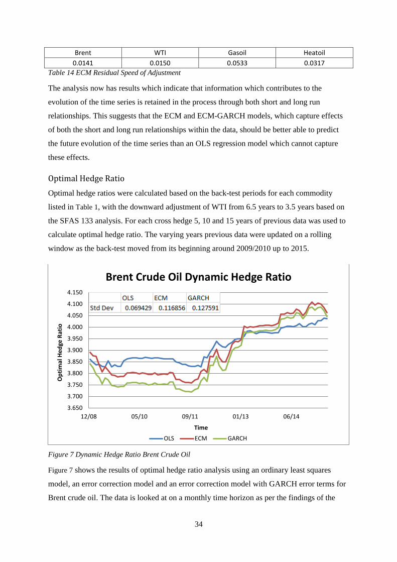
34

Brent WTI Gasoil Heatoil

0.0141 0.0150 0.0533 0.0317

Table 14 ECM Residual Speed of Adjustment

The analysis now has results which indicate that information which contributes to the

evolution of the time series is retained in the process through both short and long run

relationships. This suggests that the ECM and ECM-GARCH models, which capture effects

of both the short and long run relationships within the data, should be better able to predict

the future evolution of the time series than an OLS regression model which cannot capture

these effects.

Optimal Hedge Ratio

Optimal hedge ratios were calculated based on the back-test periods for each commodity

listed in Table 1, with the downward adjustment of WTI from 6.5 years to 3.5 years based on

the SFAS 133 analysis. For each cross hedge 5, 10 and 15 years of previous data was used to

calculate optimal hedge ratio. The varying years previous data were updated on a rolling

window as the back-test moved from its beginning around 2009/2010 up to 2015.

Figure 7 Dynamic Hedge Ratio Brent Crude Oil

Figure 7 shows the results of optimal hedge ratio analysis using an ordinary least squares

model, an error correction model and an error correction model with GARCH error terms for

Brent crude oil. The data is looked at on a monthly time horizon as per the findings of the

3.650

3.700

3.750

3.800

3.850

3.900

3.950

4.000

4.050

4.100

4.150

12/08 05/10 09/11 01/13 06/14

Op

tim

al H

ed

ge R

atio

Time

Brent Crude Oil Dynamic Hedge Ratio

OLS ECM GARCH

35

FAS 133 analysis and includes 78 observations spanning the back-test period from January

2009 to June 2015. In terms of the assertion of (Kroner & Sultan, 1993) that the OLS hedge

ratio estimation can suffer from downward bias and lead to under hedging, the results for the

Brent cross hedge do not offer conclusive evidence for or against this argument. Each of the

series track each other reasonably closely, while the ECM and ECM-GARCH models

consistently estimates a smaller hedge ratio than OLS up until 2013 after which this trend is

reversed. This may be due to the increase in correlation between Brent and jet fuel observed

around this time frame in Figure 3. The standard deviation of hedge ratio estimates for the

ECM models are larger than those of the OLS estimates. This suggests the ECM and ECM-

GARCH models are more flexible in determining optimal hedge ratio and react more to

changes in the data than the OLS approach which is consistent with the fact that these models

are more dynamic in their estimation approaches. Overall all three models produce estimates

for optimum hedge ratio which vary between 3.7 and 4.1. Since the ratios are calculated from

first differenced and jet fuel prices are in $/gallon and Brent prices in $/barrel the results

indicate that it takes between 3.7 and 4.1 barrels of jet fuel to hedge exposure to 1 gallon of

jet fuel.

Figure 8 Dynamic Hedge Ratio LS Gasoil

Illustrated in Figure 8 above are the optimal hedge ratios calculated for Gasoil using OLS,

ECM and ECM-GARCH models for data spanning a back-test period from January 2010 to

June 2015. The standard deviations of the ratios are much smaller than those of Brent, though

this would be expected as the gasoil prices are in metric-tonnes vs jet fuels in $/gallon. The

lower standard deviations (relative to hedge ratio estimations) observed in the gasoil analysis

0.025

0.026

0.027

0.028

0.029

0.03

0.031

0.032

0.033

0.034

0.035

12

/09

03

/10

06

/10

09

/10

12

/10

03

/11

06

/11

09

/11

12

/11

03

/12

06

/12

09

/12

12

/12

03

/13

06

/13

09

/13

12

/13

03

/14

06

/14

09

/14

12

/14

03

/15

Op

tim

al H

ed

ge R

atio

Time

Gasoil Dynamic Hedge Ratio

OLS ECM GARCH

36

may be attributed to the almost constant correlation between gasoil and jet fuel returns when

viewed on a monthly horizon in Figure 3.

The ECM-GARCH models incorporation of heteroscedasticity is evident from Figure 8 as we

can observe the optimal hedge ratio estimates from this model react more strongly to changes

in the data, and this is characterised by sharper adjustments in its estimated values. During

the period of falling spot prices for gasoil around the beginning of 2014 illustrated in Figure 6

the OLS estimates begin to diverge from the other two models. For the most recent years of

the back-test period the optimum hedge ratio estimates for the ECM and ECM-GARCH

models decrease slightly while the OLS estimates increase significantly. The increase in OLS

hedge ratio estimates are possibly due to an increase in volatility which one associates with

negative returns in a market downturn (Heston, 1993). The slight decrease in ECM and ECM-

GARCH estimations may be as a result of the commodity time series reacting more quickly

than expected in correcting its path towards the long run equilibrium relationship as indicated

by the data presented earlier in Table 14.

37

Hedge Performance

Hedging performance is calculated based on the minimum variance of a portfolio containing

150,000 gallons of jet fuel and the optimal number of units of the cross hedging product as

calculated by the OLS model, the ECM model and the ECM GARCH model. The optimal

number of units refers to gallons for Heatoil, barrels for Brent and WTI and metric-tonnes for

Gasoil. The equivalent number of contracts for each commodity can be calculated via

Equation 2. The reason for calculating the optimal hedging position in units of the cross-

hedging product is to obtain the most accurate results for the P&L variance analysis – so it is

assumed for the analysis that partial amounts of contracts may be purchased. For example if

the ECM model estimates it will take 3860 barrels of Brent (3.86 contracts) to hedge jet fuel

exposure on a particular month, this value is not rounded to the closest whole number of

contracts. This is because each of the model estimates will be relatively close to each other –

as shown in the previous section - and rounding them all to the nearest whole number would

obviously nullify the analysis.

The methodology surrounding the purchase of incomplete numbers of contracts represents a

limitation of the model which is not consistent with the reality of hedging and one of the

assumptions of Black-Scholes - namely that the hedger can only buy whole numbers of

contracts. For each of the commodities tested the amount of historical data used to calculate

the optimal hedge ratio for each of the three models was varied between 5, 10 and 15 years.

The analysis was also carried across a number of hedge horizons – 1, 3, 6, 9 and 12 months

for Brent and Gasoil and 1, 2, 3 and 4 quarters for WTI and Heatoil. The three lowest

variances in the analysis for each commodity are highlighted in green in Table 15, Table 16,

Table 17 and Table 18 with the lowest annualised variance overall also underlined. The

annualised variances listed are in US Dollars.

38

Brent Crude Oil

Back-test Window

OLS ECM GARCH Unhedged Hedge

Horizon

5

32,362 33,511 33,874 80,128 1M

32,653 33,853 34,222 80,411 3M

32,945 34,119 34,525 79,831 6M

32,931 33,836 34,274 71,735 9M

31,967 32,722 33,177 70,536 12M

10

32,330 32,547 32,388 80,128 1M

32,614 32,849 32,684 80,411 3M

32,924 33,157 32,986 79,831 6M

32,941 33,085 32,923 71,735 9M

31,994 32,087 31,930 70,536 12M

15

32,178 32,132 31,982 80,128 1M

32,456 32,419 32,263 80,411 3M

32,760 32,713 32,549 79,831 6M

32,783 32,671 32,515 71,735 9M

31,836 31,679 31,533 70,536 12M

Table 15 Minimum Variance Hedge Analysis Brent

Presented in Table 15 above are the back-testing results for a portfolio containing 150,000

gallons of Gulf54 grade jet fuel and a corresponding amount of Brent crude oil determined by

each of the three fuel hedging models. The figures represent the annualised variance for each

cross-hedge calculated from Equation 6. In all cases the variances of the hedged position is far

lower than the variances of the unhedged exposure to jet fuel price fluctuations. The

unhedged exposures also have a much greater deviation moving between 70 and 80 thousand

dollars whereas the variances of the hedged portfolios ranges between just 31.5 and 34

thousand dollars. The results support the assertion that hedging not only reduces portfolio

variance conditional on its underlying assets but also reduces its unconditional variance. The

effect of varying the hedge horizon also has an effect of the portfolio P&L with the 1 month

and 12 month horizons producing the lowest portfolio variance for each of the data ranges

employed which suggests that the model is better at predicting ratios for 12 months-time than

for intermediate time periods.

The results also follow an interesting trend surrounding the amount of data used for back-

testing. When using 5 years of data to calculate the optimal hedge ratio for each model the

OLS analysis produces better results that the ECM and ECM GARCH models. However the

results suggest that as the amount of data used for calculating optimal hedge ratio is expanded

to 10 and 15 years the more complex ECM and ECM GARCH models approach and

39

eventually overtake the OLS model in terms of hedge performance with the ECM GARCH

model producing the lowest overall portfolio variance for Brent crude oil when hedging on a

12 month horizon. This suggests that the ECM and ECM-GARCH models are able to form

progressively better optimal hedge ratio predictions based on an expanding data set which the

models are fitted to. This is supported by (Alexander, 2008) who states that GARCH models

based on too few observations may lack robustness which is likely the reason the ECM

GARCH eventually proves to provide the best performing hedge as the number of

observations on which the model is based are increased. The findings of the ECM with

GARCH error terms are consistent with those of (Adams & Gerner, 2012) who determine the

ECM GARCH to be the best performing model for dynamic hedging across all four

commodities used in this study.

The lowest variances in the Jet-Brent portfolio are achieved at the 12 month horizon and are

loosely consistent with the results for Jet-Gasoil portfolio presented in Table 16 below. The

analysis on the Jet-Gasoil portfolio suggests that the greatest reduction in variance is around

the 9 and 12 month horizons. However as presented in Table 14 gasoil has a greater speed of

adjustment parameter than Brent which means that the cointegrated time series of gasoil and

jet fuel tend to correct towards their long run relationship more quickly than those of Brent

and jet fuel which may explain why the best predictions are 9 months ahead for gasoil and 12

months ahead for Brent.

40

Low Sulphur Gasoil

Back-test Window

OLS ECM GARCH Unhedged Hedge

Horizon

5

50,244 51,979 54,227 80,496 1M

49,681 51,446 53,774 80,829 3M

50,245 52,318 54,538 80,044 6M

48,389 47,922 48,854 70,698 9M

48,739 47,658 48,360 69,340 12M

10

49,797 53,041 55,606 80,496 1M

49,189 52,538 55,200 80,829 3M

49,892 53,392 55,946 80,044 6M

47,841 48,621 50,520 70,698 9M

48,145 48,249 50,015 69,340 12M

15

49,670 53,543 55,901 80,496 1M

49,056 53,059 55,505 80,829 3M

49,790 53,886 56,228 80,044 6M

47,636 48,839 50,625 70,698 9M

47,903 48,381 50,013 69,340 12M

Table 16 Minimum Variance Hedge Analysis Gasoil

The analysis of the Jet-Gasoil portfolio also shows that the P&L variance of the hedged

positions far outperform the P&L variance of an unhedged position. Unlike the previous

results the Jet-Gasoil analysis does not present any evidence that the ECM and ECM GARCH

models provide better optimal hedge ratio predictions as the amount of data input is

expanded. Although the greatest reduction in variance is observed using 15 years of data to

calculate optimal hedge ratio, there is no compelling evidence to suggest that using more data

can consistently lead to more accurate predictions of optimal hedge ratio for the Jet-Gasoil

portfolio. The results show that the OLS model forms the best predictor of optimal hedge

ratio for a Jet-Gasoil portfolio. Although based on the results there is really no difference

between the lowest variance achieved by the ECM and OLS models as the OLS performs

better by a total of $22.

The residual diagnostics carried out previously may shed some light on poorer performance

of the ECM and ECM GARCH models for the Jet-Gasoil portfolio. There is much more

evidence of a stationary trend in the gasoil residuals when compared to the other three

commodities as shown in Table 10 which suggest that the OLS regressions trend line would

provide a better fit to the Jet-Gasoil residuals than for any of the other commodities which

41

would result in the OLS model giving a closer prediction to the ECM and ECM GARCH

models for this portfolio than for the other cross-hedges analysed.

The degree of autocorrelation in the residuals would have had a much greater impact on the

gasoil analysis than on any of the other portfolios as the results of Ljung-Box Q tests for

residual autocorrelation presented in Table 11 indicate much stronger evidence of

autocorrelation in the Jet-Gasoil residual series than in the other series analysed. This likely

had the effect of making the Jet-Gasoil residuals more biased towards randomness than for

the other commodities and likely reduced the usefulness of the additional information they

would have provided to the ECM and ECM GARCH models. If this assertion is true then

transformation of the residuals as per (Cochrane & Orcutt, 1949) would likely have improved

the performance of the ECM and ECM GARCH models relative to the OLS approach.

Although Table 12 shows that the Jet-Gasoil residuals also display a much high level of

heteroscedasticity than the other cross-hedges which can be accounted for in the ECM

GARCH model it’s clear that the damaging effect of autocorrelation in the residual series has

had a greater impact on the results based on the ECM GARCH approach proving to be the

worst performing model for the Jet-Brent portfolio.

The higher levels of heteroscedasticity in the Jet-Gasoil residuals may also explain why the

trend of increasing input data to produce more accurate results is not observed in the Gasoil

cross-hedge as it is in the Brent cross-hedge, as the much stronger evidence of

heteroscedasticity means that the conditional variance of the Jet-Gasoil residuals is much

more dependent on the variances immediately preceding each point than other the better

model specification associated with including more data from 10 and 15 years in the past.

Overall the cross-hedging portfolio containing gasoil does not perform as well as the Brent

portfolio with a difference of approximately $16,000 between the best performing hedges

with each commodity. The results so far indicate the Brent is the best cross-hedging product

for jet fuel at all of the time horizons analysed and provide some contrast with the results of

(Adams & Gerner, 2012) who find that gasoil proves to be the best cross-hedging product up

to three months and is overtaken by Brent for hedge horizons greater than three months.

42

West Texas Intermediary Crude Oil

Since the SFAS analysis determined that the WTI and Heatoil hedges can only meet

regulations on a three month horizon, the size of the jet fuel position being hedged by these

commodities was increased three fold to 450,000 gallons for the analysis. This is to reflect

the jet fuel required for each three month interval being hedged every quarter.

Table 17 presents the findings from the profit and loss analysis for the Jet-WTI portfolio.

While the results regarding the annualised variance of the hedged versus the unhedged

positions is consistent with the findings for Brent and gasoil, the increase in the hedge

horizon to once per quarter has had a drastically negative impact on the overall effectiveness

of WTI as a cross-hedging product. It is notable though that the WTI price movements

displayed the lowest correlation with Jet Fuel price movements on a monthly and quarterly

horizon before the profit and loss analysis took place as shown in Figure 3 and Figure 4.

Among all of the cross-hedging products analysed in the study, WTI produced the highest

annualised variance in the hedging portfolio indicating that it is the least effective cross-

hedging product analysed.

Back-test Window

OLS ECM GARCH Unhedged Hedge

Horizon

5

163,611 158,632 161,812 303,325 1Q

159,720 155,913 157,849 313,505 2Q

161,080 157,598 159,163 329,582 3Q

170,201 167,024 168,267 206,799 4Q

10

164,740 161,216 163,836 303,325 1Q

161,063 158,552 160,298 313,505 2Q

162,446 160,157 161,615 329,582 3Q

171,540 169,592 170,657 206,799 4Q

15

164,860 161,735 164,350 303,325 1Q

161,119 158,926 160,798 313,505 2Q

162,446 160,428 162,079 329,582 3Q

171,482 169,765 171,073 206,799 4Q

Table 17 Minimum Variance Hedge Analysis WTI

The results for the Jet-WTI cross indicate the error correction model produces the best results

when hedging on a quarterly horizon. The lowest variances were produced on a hedge

horizon of 6 to 9 months and using only 5 years of data. The results indicate that the inclusion

of more data in fitting each of the models does not produce more accurate predictions of

optimal hedge ratio. This is consistent with the findings of the SFAS 133 analysis presented

43

in Figure 4 which shows that the correlation between the returns series for WTI and Jet Fuel

have been much higher in the past four years when compared the eight year period analysed.

The results suggest that even though only the previous eight years were used in the SFAS

analysis that the correlation between WTI and Jet Fuel also remained at a lower level going

back to fifteen years.

The Jet Fuel and WTI time series presented the least evidence of cointegration as shown in

Table 13 and the residual diagnostics indicated that the Jet-WTI residual series also presented

the least evidence for stationarity as well as the lowest levels of heteroscedasticity out of all

of the potential cross-hedges analysed. The low levels of cointegration may explain the poor

performance overall of WTI when compared to the P&L results for heating oil shown in Table

18, which demonstrated the second highest level of cointegration after gasoil. The residual

analysis surrounding the stationarity and heteroscedasticity tests may explain the greater

performance of the ECM over the other two models as the low degree of stationarity and

heteroscedasticity between the jet fuel and WTI time series may have detracted from the

strengths of the OLS and ECM-GARCH models.

44

Home Heating Oil

Back-test Window

OLS ECM GARCH Unhedged Hedge

Horizon

5

63,702 64,314 69,348 326,588 1Q

64,785 65,166 68,715 336,264 2Q

64,995 65,004 67,461 350,555 3Q

65,109 65,171 70,625 270,233 4Q

10

65,212 67,404 75,030 326,588 1Q

66,493 68,628 75,731 336,264 2Q

66,948 68,974 75,841 350,555 3Q

66,701 69,131 78,645 270,233 4Q

15

64,455 66,488 70,958 326,588 1Q

65,767 67,709 71,762 336,264 2Q

66,203 68,020 71,770 350,555 3Q

65,565 67,964 73,714 270,233 4Q

Table 18 Minimum Variance Hedge Analysis Heatoil

Although the unhedged variances are larger for that of home heating oil than the other

quarterly hedge using WTI, the annualised variances for the Jet-Heatoil portfolio represent a

vast improvement on the WTI hedge performance. The results show that the OLS regression

produces the lowest annualised variance across all hedge horizons, though the error

correction model does produce one of the three lowest overall variances. The Jet-Heatoil

residual series displayed the second highest overall evidence of autocorrelation and the

second lowest overall evidence of heteroscedasticity. Although the jet fuel and heating oil

time series displayed the second highest level of cointegration, the effect of autocorrelation

on the information retained in the residuals as well as the weaker effect of heteroscedasticity

likely reduced the advantage that the ECM and ECM GARCH models had in being able to

capture some of the short and long run dynamics in the relationship between the Jet Fuel and

Heatoil time series.

It’s notable that in general the differences between the estimates from each model were small

and that in reality when adding the constraint of the hedger not being able to purchase partial

numbers of contracts that the differences between the models may be nullified.

45

Conclusions

This research investigated the hedging performance of Brent crude oil, West Texas

Intermediary crude oil, low sulphur gasoil and NY Harbour home heating oil when used as

cross-hedging instruments for Gulf54 grade jet fuel. The cross hedging products were

analysed under the constraints of meeting hedge accounting standards and compared using an

OLS regression model, an error correction model and an error correction model with GARCH

error terms. In all cases the use of each of the cross hedging products reduces the hedgers risk

when compared to an unhedged long position in jet fuel, though hedging exposure on a

weekly horizon is misspecified as doing so will block the portfolio from being able to qualify

for hedge accounting status under the current regulations. For Brent crude oil and low sulphur

gasoil hedging may be carried out on a monthly time horizon, though for WTI and heating oil

this horizon must be pushed out to three months in order to meet hedge regulations.

The results from the model performance show that the ECM-GARCH model produced the

lowest overall annualised variance for a portfolio containing 150,000 litres of Gulf54 grade

jet fuel and a Brent crude oil as a cross-hedging product. As well as this the model was

improved by expanding the amount of data used in specifying the GARCH parameters. It was

found the regular ECM model produced the best results for WTI while the OLS regression

produced the best results for gasoil and heating oil. The better than expected performance of

the OLS regression is significant but cannot be taken as substantial evidence of greater

overall performance as the effect of autocorrelation in the residuals was not accounted for

before performing analysis using the ECM and ECM-GARCH models and it’s likely that had

the residual data been transformed that it would have affected the overall results.

46

Bibliography Adams, Z., 2015. EVIEWS OLS, ECM & ECM GARCH Results. s.l.:Eviews File.

Adams, Z. & Gerner, M., 2012. Cross hedging jet-fuel price exposure. Energy

Economics, Volume 34, pp. 1301-1309.

Alexander, C., 2008. Practical Financial Econometrics. 1 ed. West Sussix: John Wiley &

Sons.

Alexander, C., 2008. Quantitative Methods in Finance. 1st ed. West Sussex: John Wiley

& Sons.

Anderson, R., 1954. The problem of autocorrelation in regression analysis. Journal of the

American Statistical Association, 49(265), pp. 113-129.

Anderson, R. & Danthine, J., 1981. Cross Hedging. The Journal of Political Economy,

86(6), pp. 1182-1196.

Baille, R. & Bollerslev, T., 1994. Cointegration, fractional cointegration and exchange

rate dynamics. The Journal of Finance, 2(49), pp. 737-745.

Baillie, R. & Myers, R., 1991. Bivariate GARCH estimation of the optimal commodity

futures hedge. Journal of Applied Economics, 2(6), pp. 109-124.

Banerjee, A., Doldado, J., Galbraith, J. & Hendry, D., 1993. Coi-Integration, Error

Correction and the Econometric Analysis of Non-Stationary Data. 1st ed. New York:

Oxford University Press.

Benninga, S., Eldor, R. & Zilcha, I., 1983. Optimal hedging in the futures market under

price uncertainty. Economics Letters, 2(13), pp. 141-145.

Benninga, S., Eldor, R. & Zilcha, I., 1984. The optimal hedge ratio in unbiased futures

markets. Journal of futures markets, 2(4), pp. 155-159.

Bollerslev, T., 1986. Generalized Autoregressive Conditional Heteroskedasticity. Journal

of Econometrics, 3(31), pp. 307-327.

Box, G. & Pierce, D., 1970. Distribution of residual autocorrelations in autoregressive-

integrated moving average time series models. Journal of the American statistical

Association, 65(332), pp. 1509-1526.

Byström, H., 2003. The hedging performance of electricity futures on the Nordic power

exchange. Applied Economics, 1(35), pp. 1-11.

Carter, D., Rogers, D. & Simkins, B., 2004. Fuel Hedging in the Airline Industry: The

Case of Southwest Airlines, Oklahoma: Oklahoma State University.

Carter, D., Rogers, D. & Simkins, B., 2006. Does hedging affect firm value? Evidence

from the US airline industry. Financial Management, pp. 53-86.

47

Cecchetti, S., Cumby, R. & Figlewski, S., 1988. Estimation of the Optimal Futures

Hedge. The Review of Economics and Statistics, 70(4), pp. 623-630.

Charnes, J., Koch, P. & Berkman, H., 2003. Measuring hedge effectiveness for FAS 133

compliance. Journal of applied corporate finance, 4(15), pp. 95-103.

Chou, W., Fan Denis, K. & Lee, C., 1997. Hedging with the Nikkei Index Futures: The

Convential Model versus the Error Correction Model. The Quarterly Review of

Economics and Finance, 4(36), pp. 495-505.

Clark, E., Tan, M. & Tunaru, R., 2003. Cross hedging jet fuel on the Singapore spot

market. International Journal of Banking and Finance, 1(2).

CMEGroup, 2015. CME GRoup Energy Trading, Chicago: CME Group Inc.

Cobbs, R. & Wolf, A., 2004. Jet fuel hedging strategies: options available for airlines

and a survey of industry practices. [Online]

Available at: http://www.kellogg.northwestern.edu/research/fimrc/papers/jet fuel.pdf

[Accessed 5 June 2015].

Cochrane, D. & Orcutt, G., 1949. Application of least squares regression to relationships

containing auto-correlated error terms. Journal of the American Statistical Association,

44(245), pp. 32-61.

Coffey, B., Anderson, J. & Parcell, J., 2000. Optimal Hedging Ratios and Hedging Risk

for Grain By-Product, Tampa Bay: AAEA Annual Meeting.

Conroy, R., 2003. Hedging with Forwards and Futures. [Online]

Available at:

http://faculty.darden.virginia.edu/conroyb/derivatives/Hedging%20with%20Forwards%2

0and%20Futures.pdf

[Accessed 2 July 2015].

Da-Hsiang, D., 1996. The Effect of the cointegration relationship on futures hedging: a

note. The journal of futures markets, 7(16), p. 773.

DeJong, D., Nankervis, C. & Savin, N., 1992. Integration versus Trend Stationarity in

Time Series. Journal of the Econometric Society, pp. 423-433.

Dickey, D. & Fuller, A., 1979. Distribution of the estimators for autoregressive time

series with a unit root. Journal of the American Statistical Association, 74(366a), pp. 427-

431.

Durbin, J. & Watson, G., 1950. Testing for serial correlation in least squares regression.

Biometrika, 3(37), pp. 409-428.

Ederington, L., 1979. The hedging performance of the new futures markets. The Journal

of Finance, 1(34), pp. 157-170.

48

Engle, R., 1982. Autoregressive conditional heteroscedasticity with estimates of variance

of United Kingdom inflation. Econometrica: Journal of the Econometric Society, pp. 987-

1007.

Engle, R., 2001. GARCH 101: The use of ARCH/GARCH models in applied

econometrics. Journal of economic perspectives, pp. 157-168.

Engle, R. & Granger, C., 1987. Co-integration and error correction: representation,

estimation, and testing. Econometrica: journal of the Econometric Society , pp. 251-276.

Engle, R. & Granger, C., 1987. Co-integration and error correction: representation,

estimation, and testing. Econometrica: journal of the Econometric Society , pp. 251-276.

FASB, 1998. Statement of Financial Accounting Standards No. 133, Connecticut:

Financial Accounting Standards Board.

FASC, 2008. Recommendations on Hedge accounting and accounting for transfers of

financial instruments, s.l.: Financial Accounting Standards Committee.

Figlewski, S., 1984. Hedging performance and basis risk in stock index futures. Journal

of Finance, pp. 657-669.

Ghosh, A., 1993. Hedging with stock index futures: Estimation and forecasting with error

correction model. Journal of Futures Markets, 7(13), pp. 743-752.

Granger, C., 1986. Developments in the study of cointegrated economic variable. Oxford

Bulletin of economics and statistics, 3(48), pp. 213-228.

Granger, C. & Newbold, P., 1974. Spurious regressions in econometrics. Journal of

Econometrics, 2(2), pp. 111-120.

Hansen, P. & Lunde, A., 2005. A forecast comparison of volatility models: does anything

beat a GARCH (1, 1)?. Journal of applied econometrics, 7(20), pp. 873-889.

Heston, S., 1993. A closed-form solution for options with stochastic volatility with

applications to bond and currency options. Review of financial studies, 2(6), pp. 327-343.

Hull, J., 2015. Options, futures, and Other Derivatives. 9th ed. New Jersey: Pearson

Education, Inc..

Johansen, S., 1991. Estimation and hypothesis testing of co-integration vectors in

Gaussian vector autoregressive models. Econometrica: Journal of the Econometric

Society, pp. 1551-1580.

Juhl, T., Kawaller, I. & Koch, P., 2012. The Effect of the Hedging Horizon on Optimal

Hedge Size and Effectiveness when Prices are Co-integrated. Journal of Futures Markets,

9(32), pp. 837-876.

49

Kroner, K. & Sultan, J., 1993. Time-varying distributions and dynamic hedging with

foreign currency futures. Journal of Financial and Quantitative Analysis, 4(28), pp. 535-

551.

Kwiatkowski, D., Phillips, P., Schmidt, P. & Shin, Y., 1992. Testing the null hypothesis

of stationarity against the alternative of a unit root: How sure are we that economic time

series have a unit root?. Journal of Econometrics, 1(54), pp. 159-178.

Lien, D., Tse, Y. & Tsui, K., 2002. Evaluating the hedging performance of the constant-

correlation GARCH model. Applied Financial Economics, 11(12), pp. 791-798.

Morrell, P. & Swan, W., 2006. Airline jet fuel hedging: theory and practice. Transport

Reviews, 6(26), pp. 713-730.

Myers, R. & Thompson, S., 1989. Generalized Optimal Hedge Ratio Estimation.

American Journal of Agricultural Economics, pp. 858-868.

Nelson, C. & Plosser, C., 1982. Trends and random walks in macroeconmic time series:

some evidence and implications. Journal of monetary economics, 2(10), pp. 139-162.

Silvennoinen, A. & Thorp, S., 2013. Financialization, crisis and commodity correlation

dynamics. Journal of International Financial Markets, Institutions and Money, 1(24), pp.

42-65.

Stock, J., 1987. Asymptotic properties of least squares estimators of cointegrating vectors.

Econometrica: Journal of the Econometric Society, pp. 1035-1056.

Stock, J. & Watson, M., 1988. Testing for Common Trends. Journal of the American

Statistical Association, 83(404), pp. 1097-1107.

Transtats, 2015. Airline Fuel Cost and Consumption. [Online]

Available at: www.transtats.bts.gov/fuel.asp?pn=1

[Accessed 24 August 2015].

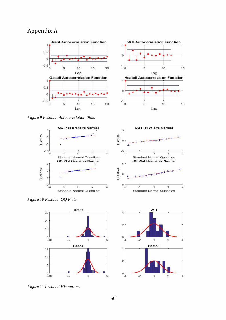
50

Appendix A

Figure 9 Residual Autocorrelation Plots

Figure 10 Residual QQ Plots

Figure 11 Residual Histograms

51

Appendix B

MATLAB Import Data

addpath(genpath('C:\Users\Niall\Documents\College\Masters\Dissertation\Data')); % add

selected folders and subfolders to path

DAILY = readtable('EIADAILY.csv'); % read in data

WEEKLY = readtable('EIAWEEKLY.csv');

MONTHLY = readtable('EIAMONTHLY.csv');

QUARTERLY = readtable('EIAQUARTERLY.csv');

MATLAB Define Parameters

COMM = 2; %2 = BRENT; 3 = WTI; 4 = GAS; 5 = HEAT

HOR = 1; % futures horizon in months

GAL = 150000; % no of gallons of Jet Fuel to Hedge

WIN = 15; % rolling window in years from which to calculate optimal hedge ratio

MATLAB Loop Arguments

if COMM == 3

LOOP = 3;

elseif COMM == 5

LOOP = 5;

else LOOP = 1;

end

% WTI & Heatoil both using quarterly prices vs. Brent and Gasoil both using monthly prices

% this is to save space repeating each loop 3 times - i.e. can use 'if COMM=LOOP, else'

% and avoid having to say 'if 3,elseif 5, else'

MATLAB SFAS 133

TH = [WIN,WIN,WIN,WIN]; %time horizons matrix

BT = [6.5 3 5.5 3.5]; % max backtest horizons as per SFAS 133

% Weekly Horizon

WEEKLY_DBL = table2array(WEEKLY(:,2:end)); % convert data series to double

WEEKLY_RETS = price2ret(WEEKLY_DBL); % convert to 15 years of returns

RSQW = zeros(1,4); % matrix to store R_Square Values for weekly horizon

LW = length(WEEKLY_RETS); % W to denote weekly

% fit linear regression

for k = 2:5

BTW = BT(1,k-1)*52; %length of SFAS back test & reset to match commodity on each loop

SFASW = (WEEKLY_RETS(LW-BTW:end,:)); %create matrix for SFAS horizon & resize on each

loop

FAS133W = fitlm(SFASW(:,1),SFASW(:,k));

RSQW(1,k-1) = FAS133W.Rsquared.Adjusted;

end

% Monthly Horizon

MONTHLY_DBL = table2array(MONTHLY(:,2:end)); % convert data series to double

MONTHLY_RETS = price2ret(MONTHLY_DBL);

RSQM = zeros(1,4); %matrix to store R_Square Values for monthly horizon

LM = length(MONTHLY_RETS);

52

for k = 2:5

BTM = BT(1,k-1)*12; %length of SFAS back test & reset to match commodity on each loop

SFASM = (MONTHLY_RETS(LM-BTM:end,:)); %create matrix for SFAS horizon & resize on each

loop

FAS133M = fitlm(SFASM(:,1),SFASM(:,k));

RSQM(1,k-1) = FAS133M.Rsquared.Adjusted;

end

% Quarterly Horizon

QUARTERLY_DBL = table2array(QUARTERLY(:,2:end)); % convert data series to double

QUARTERLY_RETS = price2ret(QUARTERLY_DBL);

RSQQ = zeros(1,4); %matrix to store R_Square Values for monthly horizon

LQ = length(QUARTERLY_RETS);

for k = 2:5

BTQ = BT(1,k-1)*4; %length of SFAS back test & reset to match commodity on each loop

SFASQ = (QUARTERLY_RETS(LQ-BTQ:end,:)); %create matrix for SFAS horizon & resize on each

loop

FAS133Q = fitlm(SFASQ(:,1),SFASQ(:,k));

RSQQ(1,k-1) = FAS133Q.Rsquared.Adjusted;

end

MATLAB Unit Root Analysis

DAILY_DBL = table2array(DAILY(:,2:end)); % first perform on levelled time series

% Augmented Dickey Fuller Test

ADF_LEVELS = zeros(4,5); %unit root levels results matrix

for i = 1:5

[h,pValue,stat,cValue] = adftest(DAILY_DBL(:,i)); % null = unit root present

ADF_LEVELS(1,i) = h;

ADF_LEVELS(2,i) = pValue; % default significance level = 0.05

ADF_LEVELS(3,i) = stat;

ADF_LEVELS(4,i) = cValue;

end

Variables = {'h';'pValue';'stat';'cValue'};

JET = ADF_LEVELS(:,1);

BRENT = ADF_LEVELS(:,2);

WTI = ADF_LEVELS(:,3);

GAS = ADF_LEVELS(:,4);

HEAT = ADF_LEVELS(:,5);

ADF_LVLTable = table(JET,BRENT,WTI,GAS,HEAT,'RowNames',Variables);

% Kwiatkowski-Phillips-Schmidt-Shin test

KPSS_LEVELS = zeros(4,5);

for i = 1:5

[h,pValue,stat,cValue] = kpsstest(DAILY_DBL(:,i));% null = stationary

KPSS_LEVELS(1,i) = h;

KPSS_LEVELS(2,i) = pValue;% default significance level = 0.05

KPSS_LEVELS(3,i) = stat;

KPSS_LEVELS(4,i) = cValue;

end

JET = KPSS_LEVELS(:,1);

BRENT = KPSS_LEVELS(:,2);

WTI = KPSS_LEVELS(:,3);

GAS = KPSS_LEVELS(:,4);

HEAT = KPSS_LEVELS(:,5);

KPSS_LVLTable = table(JET,BRENT,WTI,GAS,HEAT,'RowNames',Variables);

% perform tests on first differences

DAILY_DIFF = diff(DAILY_DBL);

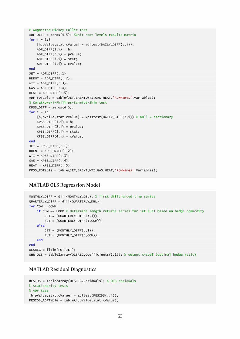
53

% Augmented Dickey Fuller Test

ADF_DIFF = zeros(4,5); %unit root levels results matrix

for i = 1:5

[h,pValue,stat,cValue] = adftest(DAILY_DIFF(:,i));

ADF_DIFF(1,i) = h;

ADF_DIFF(2,i) = pValue;

ADF_DIFF(3,i) = stat;

ADF_DIFF(4,i) = cValue;

end

JET = ADF_DIFF(:,1);

BRENT = ADF_DIFF(:,2);

WTI = ADF_DIFF(:,3);

GAS = ADF_DIFF(:,4);

HEAT = ADF_DIFF(:,5);

ADF_FDTable = table(JET,BRENT,WTI,GAS,HEAT,'RowNames',Variables);

% Kwiatkowski-Phillips-Schmidt-Shin test

KPSS_DIFF = zeros(4,5);

for i = 1:5

[h,pValue,stat,cValue] = kpsstest(DAILY_DIFF(:,i));% null = stationary

KPSS_DIFF(1,i) = h;

KPSS_DIFF(2,i) = pValue;

KPSS_DIFF(3,i) = stat;

KPSS_DIFF(4,i) = cValue;

end

JET = KPSS_DIFF(:,1);

BRENT = KPSS_DIFF(:,2);

WTI = KPSS_DIFF(:,3);

GAS = KPSS_DIFF(:,4);

HEAT = KPSS_DIFF(:,5);

KPSS_FDTable = table(JET,BRENT,WTI,GAS,HEAT,'RowNames',Variables);

MATLAB OLS Regression Model

MONTHLY_DIFF = diff(MONTHLY_DBL); % first differenced time series

QUARTERLY_DIFF = diff(QUARTERLY_DBL);

for COM = COMM

if COM == LOOP % determine length returns series for Jet Fuel based on hedge commodity

JET = (QUARTERLY_DIFF(:,1));

FUT = (QUARTERLY_DIFF(:,COM));

else

JET = (MONTHLY_DIFF(:,1));

FUT = (MONTHLY_DIFF(:,COM));

end

end

OLSREG = fitlm(FUT,JET);

OHR_OLS = table2array(OLSREG.Coefficients(2,1)); % output x-coef (optimal hedge ratio)

MATLAB Residual Diagnostics

RESIDS = table2array(OLSREG.Residuals); % OLS residuals

% stationarity tests

% ADF test

[h,pValue,stat,cValue] = adftest(RESIDS(:,4));

RESIDS_ADFTable = table(h,pValue,stat,cValue);

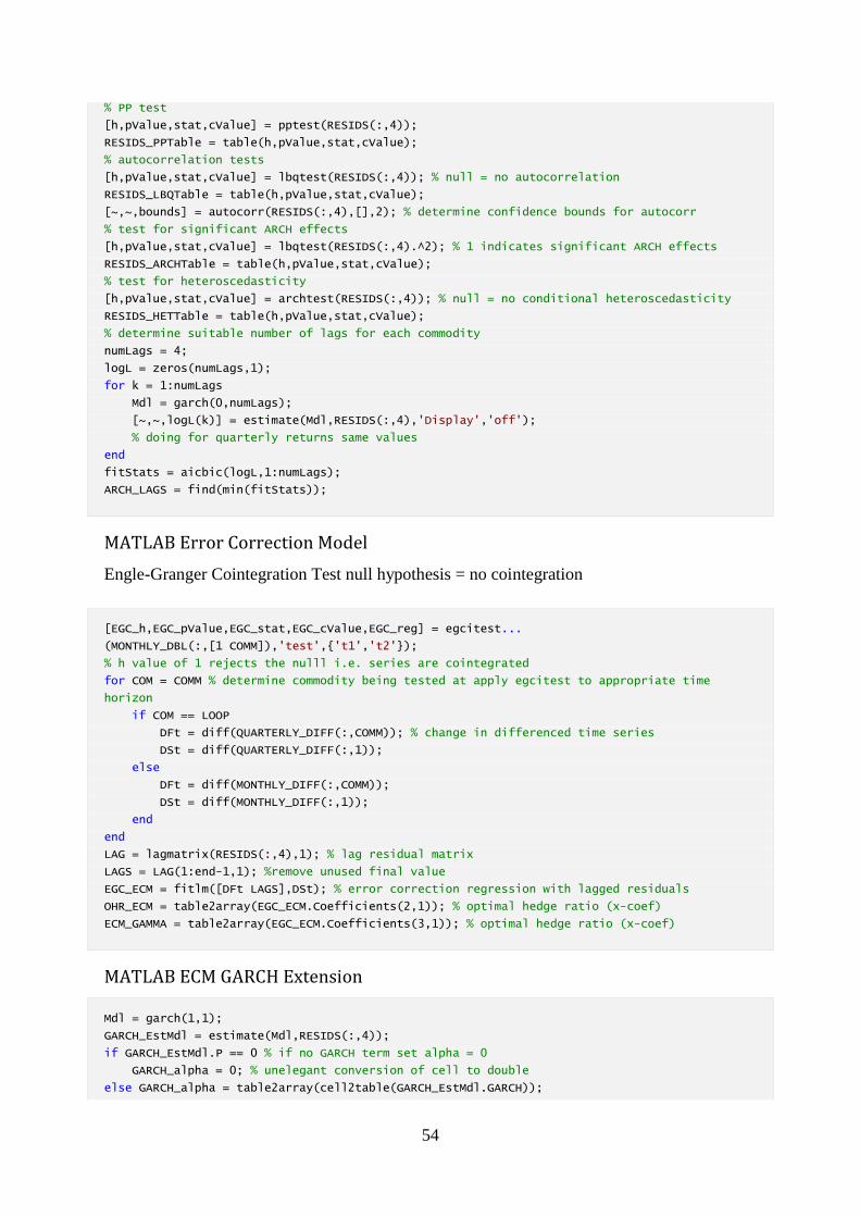
54

% PP test

[h,pValue,stat,cValue] = pptest(RESIDS(:,4));

RESIDS_PPTable = table(h,pValue,stat,cValue);

% autocorrelation tests

[h,pValue,stat,cValue] = lbqtest(RESIDS(:,4)); % null = no autocorrelation

RESIDS_LBQTable = table(h,pValue,stat,cValue);

[~,~,bounds] = autocorr(RESIDS(:,4),[],2); % determine confidence bounds for autocorr

% test for significant ARCH effects

[h,pValue,stat,cValue] = lbqtest(RESIDS(:,4).^2); % 1 indicates significant ARCH effects

RESIDS_ARCHTable = table(h,pValue,stat,cValue);

% test for heteroscedasticity

[h,pValue,stat,cValue] = archtest(RESIDS(:,4)); % null = no conditional heteroscedasticity

RESIDS_HETTable = table(h,pValue,stat,cValue);

% determine suitable number of lags for each commodity

numLags = 4;

logL = zeros(numLags,1);

for k = 1:numLags

Mdl = garch(0,numLags);

[~,~,logL(k)] = estimate(Mdl,RESIDS(:,4),'Display','off');

% doing for quarterly returns same values

end

fitStats = aicbic(logL,1:numLags);

ARCH_LAGS = find(min(fitStats));

MATLAB Error Correction Model

Engle-Granger Cointegration Test null hypothesis = no cointegration

[EGC_h,EGC_pValue,EGC_stat,EGC_cValue,EGC_reg] = egcitest...

(MONTHLY_DBL(:,[1 COMM]),'test',{'t1','t2'});

% h value of 1 rejects the nulll i.e. series are cointegrated

for COM = COMM % determine commodity being tested at apply egcitest to appropriate time

horizon

if COM == LOOP

DFt = diff(QUARTERLY_DIFF(:,COMM)); % change in differenced time series

DSt = diff(QUARTERLY_DIFF(:,1));

else

DFt = diff(MONTHLY_DIFF(:,COMM));

DSt = diff(MONTHLY_DIFF(:,1));

end

end

LAG = lagmatrix(RESIDS(:,4),1); % lag residual matrix

LAGS = LAG(1:end-1,1); %remove unused final value

EGC_ECM = fitlm([DFt LAGS],DSt); % error correction regression with lagged residuals

OHR_ECM = table2array(EGC_ECM.Coefficients(2,1)); % optimal hedge ratio (x-coef)

ECM_GAMMA = table2array(EGC_ECM.Coefficients(3,1)); % optimal hedge ratio (x-coef)

MATLAB ECM GARCH Extension

Mdl = garch(1,1);

GARCH_EstMdl = estimate(Mdl,RESIDS(:,4));

if GARCH_EstMdl.P == 0 % if no GARCH term set alpha = 0

GARCH_alpha = 0; % unelegant conversion of cell to double

else GARCH_alpha = table2array(cell2table(GARCH_EstMdl.GARCH));

55

end

GARCH_beta = table2array(cell2table(GARCH_EstMdl.ARCH));

GARCH_omega = GARCH_EstMdl.Constant;

GARCH_RESIDS = zeros(length(RESIDS(:,4))-1,1);

for i = 2:length(RESIDS(:,4))

GARCH_RESIDS(i-1,1) = GARCH_omega+(GARCH_alpha*(RESIDS(i,4)-RESIDS(i-1,4)))+...

(GARCH_beta*RESIDS(i,4).^2);

end

GARCH_ECM = fitlm([DFt GARCH_RESIDS],DSt); % error correction regression with lagged

residuals

OHR_GARCH = table2array(GARCH_ECM.Coefficients(2,1));

MATLAB Dynamic Hedge Ratio

DAYS = datenum('01-June-2015')-datenum('01-June-2000');

MONTHS = round(DAYS/365)*12; % count number of months

QUARTERS = round(DAYS/365)*4; % count number of quarters

% Define Backtest Parameters

for COM = COMM % commodities have different backtest horizon

if COM == 2

START = datenum('01-January-2009'); % Brent start period

COMOD = {'Brent'}; % labels for final table

elseif COM == 3

START = datenum('01-June-2012'); % WTI reduced due to hedge effectiveness tests

COMOD = {'WTI'};

elseif COM == 4

START = datenum('01-January-2010'); % Gasoil start period

COMOD = {'Gasoil'};

else START = datenum('01-January-2012'); % Heatoil start period

COMOD = {'Heatoil'};

end

end

FINISH = datenum('01-June-2015'); % sample end period

% Define Period in Months/Quarters

SAM_START = datenum('01-June-2015')-START; % period from START to June 2015 in days

SAM_FINISH = datenum('01-June-2015')-FINISH; % period from FINISH to June 2015 in days

SAM_START_M = round((SAM_START/365)*12); % define in months

SAM_FINISH_M = round((SAM_FINISH/365)*12);

SAM_START_Q = round((SAM_START/365)*4); % define in quarters

SAM_FINISH_Q = round((SAM_FINISH/365)*4);

% Calculate Dynamic Hedge Ratios

for COM = COMM % determine whether monthly or quarterly hedge horizon

if COM == LOOP % if using WTI or Heatoil

OHR_OLS_BT = zeros(1,SAM_START_Q-(SAM_FINISH_Q-1));

OHR_ECM_BT = OHR_OLS_BT;

OHR_GARCH_BT = OHR_OLS_BT;

JET_BT = zeros(length(SAM_FINISH_Q:SAM_FINISH_Q+(TH(1,COMM-1)*4)),1); %reset matrices

FUT_BT = zeros(length(SAM_FINISH_Q:SAM_FINISH_Q+(TH(1,COMM-1)*4)),1);

for k = SAM_FINISH_Q:SAM_START_Q % loop to run backtest

JET_BT = QUARTERLY_DIFF(LQ-(k+(TH(1,COMM-1)*4)):LQ-k,1); % use previous 8 years

of

% data starting at beginning of backtest period

FUT_BT = QUARTERLY_DIFF(LQ-(k+(TH(1,COMM-1)*4)):LQ-k,COMM); %using differenced

data

% OLS

OLSREG_BT = fitlm(FUT_BT,JET_BT); % OLS regression

56

OHR_OLS_BT(1,k-(SAM_FINISH_Q-1)) = table2array(OLSREG_BT.Coefficients(2,1));%

store OLS hedge ratio

% ECM

DFt = diff(FUT_BT); % delta first differences

DSt = diff(JET_BT);

RES = table2array(OLSREG_BT.Residuals(:,4));

LAG = lagmatrix(RES,1); % lagged residuals

LAGS = LAG(1:end-1,1);

ECM = fitlm([DFt LAGS],DSt);

OHR_ECM_BT(1,k-(SAM_FINISH_M-1)) = table2array(ECM.Coefficients(2,1));

% GARCH

GARCH_EstMdl = estimate(Mdl,RES);

if GARCH_EstMdl.P == 0 % if no GARCH term set alpha = 0

GARCH_alpha = 0;

else GARCH_alpha = table2array(cell2table(GARCH_EstMdl.GARCH));

end

GARCH_beta = table2array(cell2table(GARCH_EstMdl.ARCH));

GARCH_omega = GARCH_EstMdl.Constant;

GARCH_RES = zeros(length(RES)-1,1);

for i = 2:length(RES)

GARCH_RES(i-1,1) = GARCH_omega+(GARCH_alpha*(RES(i,:)-RES(i-1,:)))+...

(GARCH_beta*RES(i,:).^2);

end

GARCH_ECM = fitlm([DFt GARCH_RES],DSt);

OHR_GARCH_BT(1,k-(SAM_FINISH_M-1)) = table2array(GARCH_ECM.Coefficients(2,1));

end

else % if using Brent or Gasoil

OHR_OLS_BT = zeros(1,SAM_START_M-(SAM_FINISH_M-1));

OHR_ECM_BT = OHR_OLS_BT;

OHR_GARCH_BT = OHR_OLS_BT;

JET_BT = zeros(length(SAM_FINISH_M:SAM_FINISH_M+(TH(1,COMM-1)*12)),1); %reset

matrices

FUT_BT = zeros(length(SAM_FINISH_M:SAM_FINISH_M+(TH(1,COMM-1)*12)),1);

for k = SAM_FINISH_M:SAM_START_M % note change from quarterly to monthly horizon

% OLS

JET_BT = MONTHLY_DIFF(LM-(k+(TH(1,COM-1)*12)):LM-k,1);

FUT_BT = MONTHLY_DIFF(LM-(k+(TH(1,COM-1)*12)):LM-k,COMM);

OLSREG_BT = fitlm(FUT_BT,JET_BT);

OHR_OLS_BT(1,k-(SAM_FINISH_M-1)) = table2array(OLSREG_BT.Coefficients(2,1));

% ECM

DFt = diff(FUT_BT);

DSt = diff(JET_BT);

RES = table2array(OLSREG_BT.Residuals(:,4));

LAG = lagmatrix(RES,1);

LAGS = LAG(1:end-1,1);

ECM = fitlm([DFt LAGS],DSt);

OHR_ECM_BT(1,k-(SAM_FINISH_M-1)) = table2array(ECM.Coefficients(2,1));

% GARCH

GARCH_EstMdl = estimate(Mdl,RES);

if GARCH_EstMdl.P == 0 % if no GARCH term set alpha = 0

GARCH_alpha = 0;

else GARCH_alpha = table2array(cell2table(GARCH_EstMdl.GARCH));

end

GARCH_beta = table2array(cell2table(GARCH_EstMdl.ARCH));

GARCH_omega = GARCH_EstMdl.Constant;

GARCH_RES = zeros(length(RES)-1,1);

for i = 2:length(RES)

57

GARCH_RES(i-1,1) = GARCH_omega+(GARCH_alpha*(RES(i,:)-RES(i-1,:)))+...

(GARCH_beta*RES(i,:).^2);

end

GARCH_ECM = fitlm([DFt GARCH_RES],DSt);

OHR_GARCH_BT(1,k-(SAM_FINISH_M-1)) = table2array(GARCH_ECM.Coefficients(2,1));

end

end

end

OHR_OLS_BTT = transpose(OHR_OLS_BT); % transpose optimal hedge ratio series to vertical

matrices

OHR_ECM_BTT = transpose(OHR_ECM_BT); % want this format for P&L loops

OHR_GARCH_BTT = transpose(OHR_GARCH_BT);

MATLAB Calculate P&L

for COM = COMM

if COM == LOOP

JET_PRICE = QUARTERLY_DBL(LQ-(SAM_START_Q-1):end,1);

FUT_PRICE = QUARTERLY_DBL(LQ-(SAM_START_Q-1):end,COMM);

P = 4; % time periods for annualising variances

GAL = GAL*3; % triple fuel consumption on quarterly horizon

else

JET_PRICE = MONTHLY_DBL(LM-(SAM_START_M-1):end,1);

FUT_PRICE = MONTHLY_DBL(LM-(SAM_START_M-1):end,COMM);

P = 12; % time periods for annualising variances

end

end

JET_PL = zeros(length(JET_PRICE)-HOR,1);

FUT_PL_OLS = JET_PL; % reset matrix sizes for P&L

TOTAL_PL_OLS = JET_PL;

FUT_PL_ECM = JET_PL;

TOTAL_PL_ECM = JET_PL;

FUT_PL_GARCH = JET_PL;

TOTAL_PL_GARCH = JET_PL;

%calculate P&L for chosen commodity

for i = 1:length(JET_PRICE)- HOR

JET_PL(i,1) = (JET_PRICE(i,1)-JET_PRICE(i+1,1))*GAL; % JET P&L: t1-t0*gallons

N_OLS = OHR_OLS_BTT(i,1)*GAL; % number of units of futures to buy

FUT_PL_OLS(i,1) = (FUT_PRICE(i+1,1)-FUT_PRICE(i,1))*N_OLS; % FUT P&L: t0-t1*units bought

TOTAL_PL_OLS(i,1) = JET_PL(i,1) + FUT_PL_OLS(i,1); %JET P&L + FUT P&L

N_ECM = OHR_ECM_BTT(i,1)*GAL; % repeat for ECM hedge ratios

FUT_PL_ECM(i,1) = (FUT_PRICE(i+1,1)-FUT_PRICE(i,1))*N_ECM;

TOTAL_PL_ECM(i,1) = JET_PL(i,1) + FUT_PL_ECM(i,1);

N_GARCH = OHR_GARCH_BTT(i,1)*GAL; % repeat for GARCH hedge ratios

FUT_PL_GARCH(i,1) = (FUT_PRICE(i+1,1)-FUT_PRICE(i,1))*N_GARCH;

TOTAL_PL_GARCH(i,1) = JET_PL(i,1) + FUT_PL_GARCH(i,1);

end

VAR_JET = std(JET_PL)*sqrt(P); % unhedged variance

VAR_OLS = std(TOTAL_PL_OLS)*sqrt(P); % OLS variance

VAR_ECM = std(TOTAL_PL_ECM)*sqrt(P); % ECM variance

VAR_GARCH = std(TOTAL_PL_GARCH)*sqrt(P); % GARCH variance

% store & output minimum variance hedge ratio results in table

VAR = table(VAR_OLS,VAR_ECM,VAR_GARCH,VAR_JET,HOR,WIN,'RowNames',COMOD);

Published with MATLAB® R2015a