NFL 2013 Combine Data Multivariate Analysis

NFL 2013 Combine Data Multivariate Analysis

John Michael Croft, Brian Ginburg, Gary Keller and William Ward

Kennesaw State University

Page 1 of 31

Abstract

The purpose of this research is to examine the difference in multiple response variables

between groups of player positions via multivariate methods. Due to exploratory analyses and

data cleansing seeking to reduce multicolinearity among response variables, the final analysis

suggests multivariate normality reducing the probability of Type I errors when compared with a

series of univariate analyses of variances. The analysis provides strong evidence of significant

differences between groups across multiple response variables. Contrasts are utilized to highlight

the most significant differences between Group1 (FS; SS; CB; WR) vs Group 3 (OT; OC; OG;

DT) in response variables: Hands, Bench, Vertical (-.7inches, -11.87 reps, 8.7 inches,

respectively, on average) and Group 3 (OLB, ILB, DE, TE) vs Group 4 (RB) in response

variable: Height (5.97 inches on average).

Page 2 of 31

Exploratory Multivariate Analysis of the NFL Combine Data

The purpose of this analysis is to report findings from 2013 NFL Combine data using a

multivariate approach. All charts, graphs, figures, &c… can be found in the appendices at the

end of the analysis while some have been placed within the body to emphasize the importance of

the topic being addressed. Since 1982, the NFL Combine (an invitation only event) evaluates

college football players’ physical abilities and mental awareness. NFL teams use the results to

make targeted evaluations of draft prospects. Table 1 contains the original dataset variables, a

brief description, general and specific types, and measurement units.

Player positions form the basis of this analysis. Kickers (K), Long snappers (LS), and

Punters (P) are not found in the 2013 data subset, while Quarterbacks (QB) have been omitted

due to lack of observations (n=14<20). Table A displays the initial groups (A - F) prior to the

exploratory analysis and final groups (1 - 4) after the exploratory analysis.

FS FSSS SSCB CBDE WRDT DELB LBTE TEOT OTOG OGOC OC

Group E WR DT

Group F RB Group 4 RB

Table A: Player Position Groupings

Group 2

Group B

Group C

Group D Group 3

Group A

Initial Groups Final Groups

Group 1

The initial groups above are based on an assumption that players at similar positions have

similar attributes. Tight Ends have been arbitrarily assigned to Group C primarily for group

sample size consistency as well as expecting similar attributes (e.g. height, weight, &c...). The

final groups above will be discussed later but reclassify certain positions to better align with

Page 3 of 31

adjusted expectations after the exploratory analysis. Significant differences in response variables

due to perceived group attribute differences (e.g. big v. small; fast v. slow; short v. tall) were

expected. Figure 1 shows approximately equal initial group sizes. The global hypothesis expects

significant group differences in at least one response variable.

Data Cleansing

The following variables are considered redundant or inconsequential and have

been omitted from this analysis: College, FirstName, HeightFeet, HeightInches, LastName,

Name, Pick, PickRound, PickTotal, Round, and Year.

Missing values are assumed missing at random and have been set to missing to observe

percent missing per variable and per observation (see Tables 2 & 3). Variables missing more

than 20% were omitted from the analysis: Wonderlic, TwentyYD, ThreeCone, TwentySS.

Observations missing more than 33.34% were omitted from the analysis: ID #’s 9225, 8984,

9107, 9140. All remaining missing values were imputed via linear regression (by position) due to

the Central Limit Theorem (n>30) assuming normality.

While moderate response variable correlations are desirable, significant correlations (>.7)

were examined to reduce multicolinearity and increase the power of the analysis. Table 4 shows

all possible correlations with significant correlations highlighted. All response variables, other

than Hands and Bench, are significantly correlated with at least one other response variable. In

conjunction with evaluating standardized effect sizes (Figure 2), Broad and TenYd have been

omitted from further analysis. Acknowledging FortyYD has marginally higher correlations than

TenYD, assumed industry preference is to keep FortyYD in the analysis.

Page 4 of 31

Weight Arms Hands fortyyd_2 tenyd_2 vertical_2 broad_2 bench_2HeightInc

hesTotalWeight 1 0.63631 0.5426 0.88516 0.87387 -0.75372 -0.77584 0.64951 0.71823

Arms 0.63631 1 0.53112 0.48541 0.48194 -0.33836 -0.31332 0.23887 0.76487

Hands 0.5426 0.53112 1 0.46659 0.4461 -0.31323 -0.33992 0.37235 0.5269

fortyyd_2 0.88516 0.48541 0.46659 1 0.93863 -0.8223 -0.85232 0.49038 0.55655

tenyd_2 0.87387 0.48194 0.4461 0.93863 1 -0.81002 -0.83432 0.48381 0.57244

vertical_2 -0.7537 -0.3384 -0.3132 -0.8223 -0.81 1 0.89585 -0.36448 -0.41117

broad_2 -0.7758 -0.3133 -0.3399 -0.85232 -0.8343 0.89585 1 -0.40607 -0.41073

bench_2 0.64951 0.23887 0.37235 0.49038 0.48381 -0.36448 -0.40607 1 0.2994

HeightInchesTotal 0.71823 0.76487 0.5269 0.55655 0.57244 -0.41117 -0.41073 0.2994 1

Table 4: Pearson Correlation Coefficients

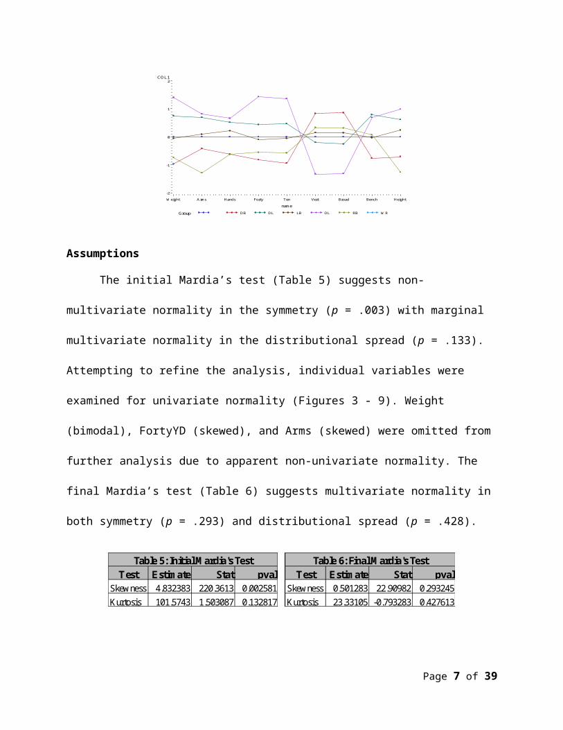
Figure 2: Initial Group Variable Profile PlotCOL1

-2

-1

0

1

2

name

Weight Arms Hands Forty Ten Vert Broad Bench Height

Group DB DL LB OL RB WR

Assumptions

The initial Mardia’s test (Table 5) suggests non-multivariate normality in the symmetry

(p = .003) with marginal multivariate normality in the distributional spread (p = .133).

Attempting to refine the analysis, individual variables were examined for univariate normality

(Figures 3 - 9). Weight (bimodal), FortyYD (skewed), and Arms (skewed) were omitted from

further analysis due to apparent non-univariate normality. The final Mardia’s test (Table 6)

suggests multivariate normality in both symmetry (p = .293) and distributional spread (p = .428).

Test Estimate Stat pvalSkewness 4.832383 220.3613 0.002581

Kurtosis 101.5743 1.503087 0.132817

Table 5: Initial Mardia's Test


Kurtosis 23.33105 -0.793283 0.427613

Table 6: Final Mardia's Test

Page 5 of 31

At this time the reader is reminded of and encouraged to review Table A, delineating the

initial groups (A - F) from the final groups (1 - 4). Figure 10 suggests concerns with variance

homogeneity between the initial groups - the Vertical boxplot is provided as an example. Other

variables’ boxplots suggest similar concerns but have been omitted as redundant. Table 7

supports nonhomogeneous variance between the initial groups (p < .001).

Players were reclassified into final groups (1-4) attemptimg to correct for non-

homogeneous variance. Group 1 is a combination of Groups A plus E; Group 2 is a combination

of Group C plus DE; Group 3 is a combination of Group D plus DT; Group 4 is the same as

Group F. Group sample sizes remain similar (Figure 11). Table 8 supports variance homogeneity

between final groups (p < .552).

Chi-Square DF Pr > ChiSq

113.146532 50 <.0001

Table 7: MVN Variance Test

Chi-Square DF Pr > ChiSq28.352169 30 0.5518


Observations are assumed independent from each other as players are measured

separately from one another (i.e. One player’s results do not influence another player’s results.)

Univariate independence is assumed suggesting multivariate independence can be assumed.

Mahalanobis distances were calculated per observation. An upper limit of 13 was

approximated using the mean and adding three standard deviations (3.9 + 3*(2.9)) to determine

outliers. Five outliers were detected but were not removed due to low marginal impact on the

analysis.

Results

Page 6 of 31

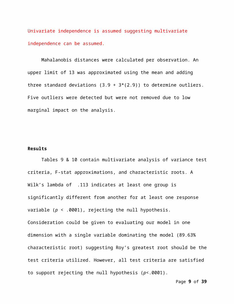
Tables 9 & 10 contain multivariate analysis of variance test criteria, F-stat

approximations, and characteristic roots. A Wilk’s lambda of .113 indicates at least one group is

significantly different from another for at least one response variable (p < .0001), rejecting the

null hypothesis. Consideration could be given to evaluating our model in one dimension with a

single variable dominating the model (89.63% characteristic root) suggesting Roy’s greatest root

should be the test criteria utilized. However, all test criteria are satisfied to support rejecting the

null hypothesis (p<.0001).

Statistic Value F Value Num DF Den DF Pr > FWilks' Lambda 0.1125846 74.43 12 696.12 <.0001Pillai's Trace 1.2195636 45.38 12 795 <.0001Hotelling-Lawley Trace

5.1503363 112.51 12 455.96 <.0001

Roy's Greatest Root 4.6160624 305.81 4 265 <.0001

Table 9: MANOVA Test Criteria & F Approximations

NOTE: F Statistic for Roy's Greatest Root is an upper bound.

Univariate analyses of variances were analyzed per response variables (Table 11). The

univariate results indicate significant differences between groups per response variable,

suggesting contrasts be analyzed per response variable.

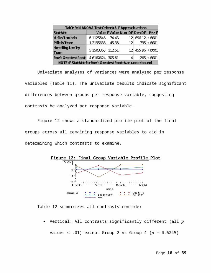
Figure 12 shows a standardized profile plot of the final groups across all remaining

response variables to aid in determining which contrasts to examine.

Figure 12: Final Group Variable Profile PlotCOL1

-2

-1

0

1

name

Hands Vert Bench Height

group_2 DB/WRLB/DE/TE OL/DTRB

Table 12 summarizes all contrasts consider:

Page 7 of 31

Vertical: All contrasts significantly different (all p values ≤ .01) except Group 2

vs Group 4 (p = 0.6245) with Group 1 vs Group 3 being most significant (SS =

2970.98, Estimate = 8.70).

Bench: All contrasts significantly different (all p values < .0001) except Group 2

vs Group 3 (p = .468) with Group 1 vs Group 3 being most significant (SS =

5474.55, Estimate = -11.81).

Hands: All contrasts significantly different (all p values ≤ .0243) except Group 2

vs Group 3 (p = .6897) with Group 1 vs. Group 3 being most significant (SS =

19.18, Estimate = -0.70).

Height: All contrasts significantly different (all p values ≤ .0012) with Group 3

vs. Group 4 being most significant (SS = 874.20, Estimate = 5.97).

Contrast Contrast SS Estimate Pr > FDB/WR vs LB/DE/TE 149.132746 1.9346678 <.0001

DB/WR vs OL/DT 2970.979953 8.69776183 <.0001

DB/WR vs RB 72.29268 1.67462185 0.0014

LB/DE/TE vs OL/DT 1692.05026 6.76309403 <.0001

LB/DE/TE vs RB 1.675503 -0.260046 0.6245

OL/DT vs RB 1211.140559 -7.02314 <.0001

DB/WR vs LB/DE/TE 2159.701381 -7.3623549 <.0001

DB/WR vs OL/DT 5474.545985 -11.806786 <.0001

DB/WR vs RB 1132.773171 -6.6288939 <.0001

LB/DE/TE vs OL/DT 730.726452 -4.4444314 <.0001

LB/DE/TE vs RB 13.329045 0.733461 0.4677

OL/DT vs RB 658.321367 5.1778925 <.0001

DB/WR vs LB/DE/TE 10.55147097 -0.5146078 <.0001

DB/WR vs OL/DT 19.17916754 -0.6988316 <.0001

DB/WR vs RB 0.03911035 0.03895072 0.6897

LB/DE/TE vs OL/DT 1.25549104 -0.1842237 0.0243

LB/DE/TE vs RB 7.59227804 0.55355856 <.0001

OL/DT vs RB 13.36559713 0.7377823 <.0001

DB/WR vs LB/DE/TE 332.3727022 -2.8882353 <.0001

DB/WR vs OL/DT 606.3480271 -3.9293312 <.0001

DB/WR vs RB 107.0115459 2.03744038 <.0001

LB/DE/TE vs OL/DT 40.0962606 -1.0410959 0.0012

LB/DE/TE vs RB 601.1413339 4.92567568 <.0001

OL/DT vs RB 874.1998387 5.96677157 <.0001

Hei

ght

Table 12: Contrasts & Estimates

Verti

cal

Benc

hH

ands

Conclusion

Page 8 of 31

The analysis supports the expected hypothesized significant differences between groups

of 2013 NFL draft combine participants. The most significant differences are found between

Group 1 vs Group 3 (Vertical; Bench; Hands); i.e. Defensive backs and wide receivers, on

average, jump 8.7 inches higher, bench press 11.87 less reps, and have hands .7 inches less than

offensive linemen and defensive tackles. On average, this is expected due to the nature of

positions within each group – defensive backs and wide receivers are required to be more athletic

overall, running faster longer, jumping higher to catch passes while offensive linemen and

defensive tackles require stamina and stability to pass block and run block constantly coming in

contact with the opposing team.

However, the most significant difference in height is between Group 3 vs Group 4; i.e.

Running backs, on average, are 5.97 inches shorter than offensive linemen and defensive tackles.

On average, this is expected due to the nature of positions within each group – running backs are

required to be more mobile and agile to break tackles, hurdle defenders and outrun the opposing

team while offensive linemen and defensive tackles were discuss above. Additionally defensive

tackles are looking to disrupt passing attempts with maximum vertical extension utilizing the

additional 5.97 inches in height.

Overall, the analysis provide strong evidence toward significant differences between

groups primarily due to the inherent athleticism commonly found within each group allowing

similar within group performances across response variables.

Recommend offensive linemen and defensive tackles focus primarily on stamina and

stability while defensive backs, wide receivers and running backs focus more on mobility and

agility. Linebackers, defensive ends, and tight ends should attempt to focus on some combination

Page 9 of 31

of stamina, stability, mobility and agility as versatility is required at those positions; recommend

heavier players focus on stamina and stability while lighter players focus on mobility and agility.

While linear combinations were not compared, it is noted the groups somewhat achieve

this organically by grouping positions of players with similar size, weight and athleticism.

Future Research

Comparing the results of the current analysis with same players’ production over the first

2-5 years of their career may be of interest (both drafted and undrafted participants) as well as

predicting future combine participant responses. Recommend future studies focus on the

differences among drafted and undrafted combine participants per same response variables.

Additionally, focusing only on drafted combine participants would allow draft picks to be

evaluated as an additional response variable.

Appendix 1: Tables

Page 10 of 31

FS FSSS SSCB CBDE WRDT DELB LBTE TEOT OTOG OGOC OC

Group E WR DT

Group F RB Group 4 RB

Table A: Player Position Groupings

Group 2

Group B

Group C

Group D Group 3

Group A

Initial Groups Final Groups

Group 1

Variable Name Discription General Type Specific Type Measurement UnitsArms Length of Arms Quantitative Interval/Ratio InchesBench Number of 225 pound reps Quantitative Interval/Ratio Number of repsBroad Broad Jump Quantitative Interval/Ratio InchesCollege College Attended Qualitative Nominal N/AFirstName First Name Categorical Nominal N/AFortyYD 40 Yard Dash Time Quantitative Interval/Ratio SecondsHands Length of Hands Quantitative Interval/Ratio InchesHeightFeet Height in Feet Only Quantitative Interval/Ratio FeetHeightInch Height in Inches Quantitative Interval/Ratio InchesHeightInches Remaining Inches Quantitative Interval/Ratio InchesID ID Number Quantitative Identifier Variable N/ALastName Last Name Categorical Nominal N/AName Player's Name Categorical Nominal N/APick Pick Number in Round and Overall Quantitative Interval/Ratio Pick in Round (Pick in Draft)PickRound Pick Number in Draft Round Quantitative Interval/Ratio Pick Number in RoundPickTotal Overall Draft Pick Number Quantitative Interval/Ratio Pick Number in Overall DraftPosition Primary Position Categorical Nominal N/ARound Draft Round Evaluated Quantitative Interval/Ratio Round NumberTenYD First 10 Yards Quantitative Interval/Ratio SecondsThreeCone 3 Cone Drill Time Quantitative Interval/Ratio SecondsTwentySS 20 Yard Shuttle Time Quantitative Interval/Ratio SecondsTwentyYD First 20 Yards Quantitative Interval/Ratio SecondsVertical Vertical Jump Quantitative Interval/Ratio InchesWeight Weight in Pounds Quantitative Interval/Ratio PoundsWonderlic Wonderlic Intelligence Score Quantitative Interval/Ratio ScoreYear Combine Year Quantitative Interval/Ratio Year

Table 1: List of Variables in the NFL Combine Data

Page 11 of 31

Variable N N Miss % Miss Individual N N Miss % MissWonderlic 0 287 100.00% 9225 6 6 50.00%TwentyYD 8 279 97.21% 8984 7 5 41.67%ThreeCone 205 82 28.57% 9107 7 5 41.67%TwentySS 219 68 23.69% 9140 7 5 41.67%Bench 230 57 19.86% 9007 8 4 33.33%TenYD 248 39 13.59% 9012 8 4 33.33%Vertical 248 39 13.59% 9018 8 4 33.33%Broad 255 32 11.15% 9028 8 4 33.33%FortyYD 272 15 5.23% 9037 8 4 33.33%Arms 286 1 0.35% 9043 8 4 33.33%Hands 286 1 0.35% 9058 8 4 33.33%id 287 0 0.00% 9064 8 4 33.33%Year 287 0 0.00% 9065 8 4 33.33%HeightFeet 287 0 0.00% 9083 8 4 33.33%HeightInches 287 0 0.00% 9095 8 4 33.33%Weight 287 0 0.00% 9139 8 4 33.33%HeightInchesTotal 287 0 0.00% 9185 8 4 33.33%

8972 9 3 25.00%8977 9 3 25.00%9009 9 3 25.00%9175 9 3 25.00%8966 10 2 16.67%8983 10 2 16.67%9001 10 2 16.67%

Table 2: Variable Reduction (>25% missing)

Table 3: Observation Reduction(>.334 Missing)

Weight Arms Hands fortyyd_2 tenyd_2 vertical_2 broad_2 bench_2HeightInc

hesTotalWeight 1 0.63631 0.5426 0.88516 0.87387 -0.75372 -0.77584 0.64951 0.71823

Arms 0.63631 1 0.53112 0.48541 0.48194 -0.33836 -0.31332 0.23887 0.76487

Hands 0.5426 0.53112 1 0.46659 0.4461 -0.31323 -0.33992 0.37235 0.5269

fortyyd_2 0.88516 0.48541 0.46659 1 0.93863 -0.8223 -0.85232 0.49038 0.55655

tenyd_2 0.87387 0.48194 0.4461 0.93863 1 -0.81002 -0.83432 0.48381 0.57244

vertical_2 -0.7537 -0.3384 -0.3132 -0.8223 -0.81 1 0.89585 -0.36448 -0.41117

broad_2 -0.7758 -0.3133 -0.3399 -0.85232 -0.8343 0.89585 1 -0.40607 -0.41073

bench_2 0.64951 0.23887 0.37235 0.49038 0.48381 -0.36448 -0.40607 1 0.2994

HeightInchesTotal 0.71823 0.76487 0.5269 0.55655 0.57244 -0.41117 -0.41073 0.2994 1

Table 4: Pearson Correlation Coefficients


Kurtosis 101.5743 1.503087 0.132817

Table 5: Initial Mardia's Test


Kurtosis 23.33105 -0.793283 0.427613

Table 6: Final Mardia's Test

Page 12 of 31

Chi-Square DF Pr > ChiSq

113.146532 50 <.0001


Chi-Square DF Pr > ChiSq28.352169 30 0.5518


Statistic Value F Value Num DF Den DF Pr > FWilks' Lambda 0.1125846 74.43 12 696.12 <.0001Pillai's Trace 1.2195636 45.38 12 795 <.0001Hotelling-Lawley Trace

5.1503363 112.51 12 455.96 <.0001

Roy's Greatest Root 4.6160624 305.81 4 265 <.0001

Table 9: MANOVA Test Criteria & F Approximations

NOTE: F Statistic for Roy's Greatest Root is an upper bound.

vertical_2 bench_2 HandsHeightInche

sTotal4.61606237 89.63 -0.0184358 0.00785156 0.0187705 0.01626727

0.4222601 8.2 0.01059568 -0.0034606 0.0141656 0.025248150.1120138 2.17 0.01125293 0.00875417 0.0206764 -0.0031582

0 0 -0.0011242 -0.0037193 0.1251432 -0.0135694

Table 10: Characteristic Roots and Vectors

Characteristic Root PercentCharacteristic Vector V'EV=1

Variable F Value Pr > FVertical 156.76 <.0001Bench 75.01 <.0001Hands 36.46 <.0001HeightinInchesTotal 109.42 <.0001

Table 11: Univariate Analysis of Variance

Page 13 of 31

Contrast Contrast SS Estimate Pr > FDB/WR vs LB/DE/TE 149.132746 1.9346678 <.0001

DB/WR vs OL/DT 2970.979953 8.69776183 <.0001

DB/WR vs RB 72.29268 1.67462185 0.0014

LB/DE/TE vs OL/DT 1692.05026 6.76309403 <.0001

LB/DE/TE vs RB 1.675503 -0.260046 0.6245

OL/DT vs RB 1211.140559 -7.02314 <.0001

DB/WR vs LB/DE/TE 2159.701381 -7.3623549 <.0001

DB/WR vs OL/DT 5474.545985 -11.806786 <.0001

DB/WR vs RB 1132.773171 -6.6288939 <.0001

LB/DE/TE vs OL/DT 730.726452 -4.4444314 <.0001

LB/DE/TE vs RB 13.329045 0.733461 0.4677

OL/DT vs RB 658.321367 5.1778925 <.0001

DB/WR vs LB/DE/TE 10.55147097 -0.5146078 <.0001

DB/WR vs OL/DT 19.17916754 -0.6988316 <.0001

DB/WR vs RB 0.03911035 0.03895072 0.6897

LB/DE/TE vs OL/DT 1.25549104 -0.1842237 0.0243

LB/DE/TE vs RB 7.59227804 0.55355856 <.0001

OL/DT vs RB 13.36559713 0.7377823 <.0001

DB/WR vs LB/DE/TE 332.3727022 -2.8882353 <.0001

DB/WR vs OL/DT 606.3480271 -3.9293312 <.0001

DB/WR vs RB 107.0115459 2.03744038 <.0001

LB/DE/TE vs OL/DT 40.0962606 -1.0410959 0.0012

LB/DE/TE vs RB 601.1413339 4.92567568 <.0001

OL/DT vs RB 874.1998387 5.96677157 <.0001

Hei

ght

Table 12: Contrasts & Estimates

Verti

cal

Benc

hH

ands

Page 14 of 31

Appendix 2: Figures

Figure 1: Initial Group Frequency Distribution

Figure 2: Initial Group Variable Profile Plot

COL1

-2

-1

0

1

2

name

Weight Arms Hands Forty Ten Vert Broad Bench Height

Group DB DL LB OL RB WR

Figure 3: Forty Yard Time Histogram (in seconds)

Page 15 of 31

Figure 4: Weight Histogram (in pounds)

Figure 5: Bench Press Histogram (# of reps)

Figure 6: Vertical Jump Histogram (in inches)

Figure 7: Hand Length Histogram (in inches)

Page 16 of 31

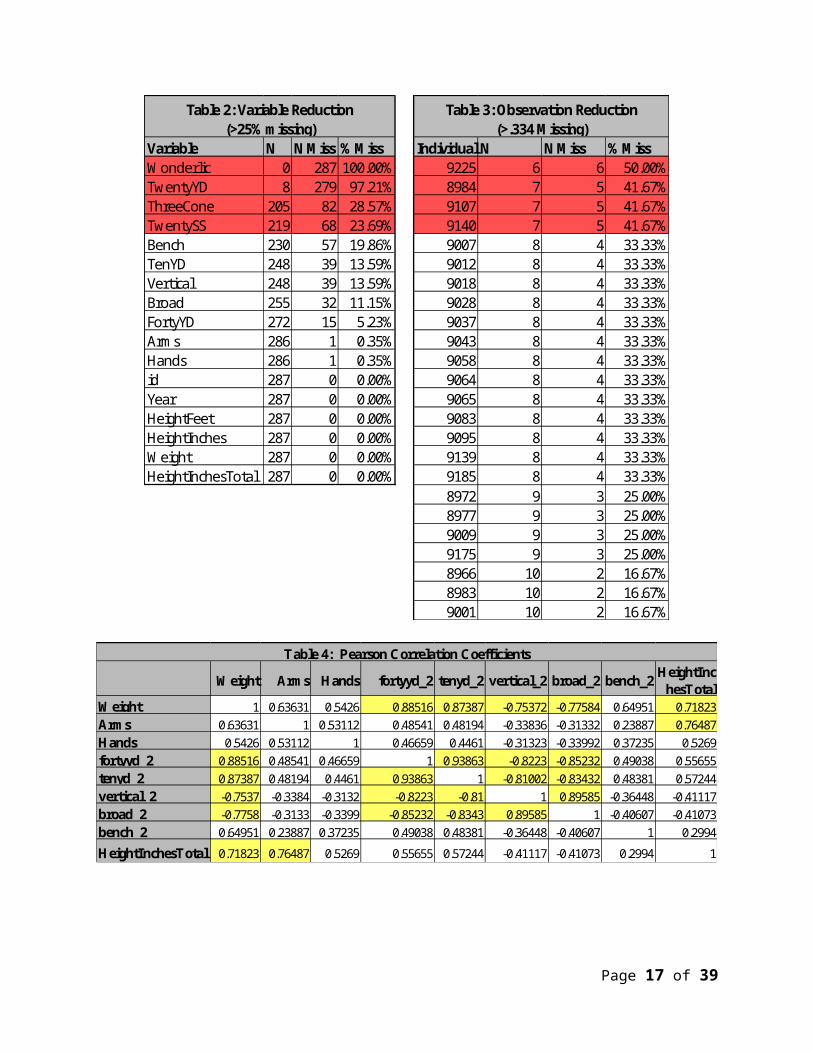
Figure 8: Height Histogram (in inches)

Figure 9: Arms Histogram (in inches)

Figure 10: Vertical Jump Boxplot (in inches)

Page 17 of 31

Figure 11: Final Group Frequency Distribution

Figure 12: Final Group Variable Profile PlotCOL1

-2

-1

0

1

name

Hands Vert Bench Height

group_2 DB/WRLB/DE/TE OL/DTRB

Appendix 3: SAS Code

Page 18 of 31

*========================================================================================================================* Create Library and Read Data to the Library *========================================================================================================================*;

libname C13 "\\Client\F$\Stat Classes\Current\Multivariate Data Analysis\Project1";

proc import datafile="\\Client\F$\Stat Classes\Current\Multivariate Data Analysis\Project1\combine.csv" out=combine dbms=csv replace; getnames=yes;run;

data C13.combine;set combine;

run;

*========================================================================================================================* Variable Audit *========================================================================================================================*;

proc means data = C13.combine;run;

*========================================================================================================================* Set all other 0 Values to missing *========================================================================================================================*;

data C13.combine_2 (drop = i);set C13.combine;

array var{*} arms hands fortyyd twentyyd tenyd twentyss threecone vertical broad bench round pickround picktotal wonderlic;

do i = 1 to 14; if var{i} = 0 then var{i} = . ;

end;run;

proc means data = C13.combine_2 n nmiss min max mean std;run;

data C13.combine_2 (drop = wonderlic twentyyd threecone twentyss);set C13.combine_2;

run;

Page 19 of 31

*========================================================================================================================* Use a transpose to identify individuals

that have several missing values. *========================================================================================================================*;

data temp (drop = college firstname lastname name pick pickround picktotal round year) ;

set C13.combine_2;run;

proc transpose data = temp out = transpose;run;

proc means data = transpose n nmiss;run;

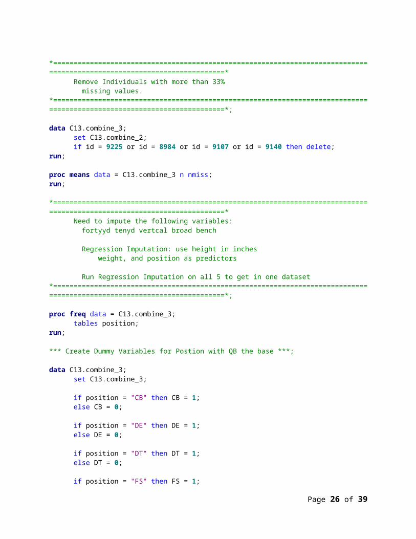
*========================================================================================================================* Remove Individuals with more than 33%

missing values. *========================================================================================================================*;

data C13.combine_3;set C13.combine_2;if id = 9225 or id = 8984 or id = 9107 or id = 9140 then delete;

run;

proc means data = C13.combine_3 n nmiss;run;

*========================================================================================================================* Need to impute the following variables:

fortyyd tenyd vertcal broad bench

Regression Imputation: use height in inchesweight, and position as predictors

Run Regression Imputation on all 5 to get in one dataset*========================================================================================================================*;

proc freq data = C13.combine_3;tables position;

run;

*** Create Dummy Variables for Postion with QB the base ***;

data C13.combine_3;set C13.combine_3;

if position = "CB" then CB = 1; else CB = 0;

Page 20 of 31

if position = "DE" then DE = 1; else DE = 0;

if position = "DT" then DT = 1; else DT = 0;

if position = "FS" then FS = 1; else FS = 0;

if position = "IL" then IL = 1; else IL = 0;

if position = "OC" then OC = 1; else OC = 0;

if position = "OG" then OG = 1; else OG = 0;

if position = "OL" then OL = 1; else OL = 0;

if position = "OT" then OT = 1; else OT = 0;

if position = "WR" then WR = 1; else WR = 0;

if position = "RB" then RB = 1; else RB = 0;

if position = "SS" then SS = 1; else SS = 0;

if position = "TE" then TE = 1; else TE = 0;

run;

*** Regression Imputation ***;

proc reg data = C13.combine_3;model fortyyd = CB DE DT FS IL OC OG OL OT WR RB SS TE / VIF;output out=impute_1 p=predicted_fortyyd;

run;quit;

proc reg data = impute_1;model tenyd = CB DE DT FS IL OC OG OL OT WR RB SS TE / VIF;output out=impute_2 p=predicted_tenyd;

run;quit;

proc reg data = impute_2;model vertical = CB DE DT FS IL OC OG OL OT WR RB SS TE / VIF;output out=impute_3 p=predicted_vertical;

run;quit;

Page 21 of 31

proc reg data = impute_3;model Broad = CB DE DT FS IL OC OG OL OT WR RB SS TE / VIF;output out=impute_4 p=predicted_broad;

run;quit;

proc reg data = impute_4;model Bench = CB DE DT FS IL OC OG OL OT WR RB SS TE / VIF;output out=impute_5 p=predicted_bench;

run;quit;

data C13.combine_Imputation_GK;set impute_5;

/*=====================================================fortyy_2, vertical_2, etc. are the imputed values

*=====================================================*/

if fortyyd = . then fortyyd_2 = predicted_fortyyd;else fortyyd_2 = fortyyd;

if tenyd = . then tenyd_2 = predicted_tenyd;else tenyd_2 = tenyd;

if vertical = . then vertical_2 = predicted_vertical;else vertical_2 = vertical;

if broad = . then broad_2 = predicted_broad;else broad_2 = broad;

if bench = . then bench_2 = predicted_bench;else bench_2 = bench;

run;

*===========================================================================================*

Remove unnecessary variable and create the groups.*==========================================================================================*;

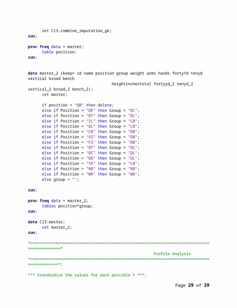
data master;set C13.combine_imputation_gk;

run;

proc freq data = master;table position;

run;

data master_2 (keep= id name position group weight arms hands fortyYd tenyd vertical broad bench

heightinchestotal fortyyd_2 tenyd_2 vertical_2 broad_2 bench_2);

Page 22 of 31

set master;

if position = "QB" then delete;else if Position = "DE" then Group = "DL"; else if Position = "DT" then Group = "DL";else if Position = "IL" then Group = "LB";else if Position = "OL" then Group = "LB";else if Position = "CB" then Group = "DB";else if Position = "SS" then Group = "DB";else if Position = "FS" then Group = "DB";else if Position = "OT" then Group = "OL";else if Position = "OC" then Group = "OL";else if Position = "OG" then Group = "OL";else if Position = "TE" then Group = "LB";else if Position = "RB" then Group = "RB";else if Position = "WR" then Group = "WR";else group = "";

run;

proc freq data = master_2;tables position*group;

run;

data C13.master;set master_2;

run;

*===========================================================================================*

Profile Analysis*==========================================================================================*;

*** Standardize the values for each possible Y ***;

proc means data = C13.master;var weight arms hands fortyyd_2 tenyd_2 vertical_2 broad_2 bench_2

heightinchestotal;output out = standard mean = avg_weight avg_arms avg_hands avg_forty

avg_ten avg_vert avg_broad avg_bench avg_height std = std_weight std_arms std_hands std_forty

std_ten std_vert std_broad std_bench std_height;run;

proc sql; create table standard_2 as select * from C13.master, standard;quit;

data standard_3 (drop= weight arms hands fortyyd_2 tenyd_2 vertical_2 broad_2 bench_2 heightinchestotal

avg_weight avg_arms avg_hands avg_forty avg_ten avg_vert avg_broad avg_bench avg_height

std_weight std_arms ste_hands std_forty std_ten std_vert std_broad std_bench std_height

Page 23 of 31

_type_ _freq_ fortyyd tenyd vertical broad bench name position id);

set standard_2;s_weight = (weight-avg_weight)/std_weight;s_arms = (arms-avg_arms)/std_arms;s_hands = (hands-avg_hands)/std_hands;s_forty = (fortyyd_2-avg_forty)/std_forty;s_ten = (tenyd_2-avg_ten)/std_ten;s_vert = (vertical_2-avg_vert)/std_vert;s_broad = (broad_2-avg_broad)/std_broad;s_bench = (bench_2-avg_bench)/std_bench;s_height = (heightinchestotal-avg_height)/std_height;

run;

*** Obtain the average of the standardized values and plot per group ***;

proc means data = standard_3;class group;var s_weight s_arms s_hands s_forty s_ten s_vert s_broad s_bench

s_height;output out = temp mean = avg_weight avg_arms avg_hands avg_forty

avg_ten avg_vert avg_broad avg_bench avg_height;run;

data temp2 (drop= _freq_ _type_);set temp;

run;

proc transpose data = temp2 out=trans;by group;

run;

proc format;value varfmt

1 = "Weight"2 = "Arms"3 = "Hands"4 = "Forty"5 = "Ten"6 = "Vert"7 = "Broad"8 = "Bench"9 = "Height";

run;

data temp3;set trans;

if _name_ = "avg_weight" then name = 1;else if _name_ = "avg_arms" then name = 2;else if _name_ = "avg_hands" then name = 3;else if _name_ = "avg_forty" then name = 4;else if _name_ = "avg_ten" then name = 5;else if _name_ = "avg_vert" then name = 6;else if _name_ = "avg_broad" then name = 7;else if _name_ = "avg_bench" then name = 8;

Page 24 of 31

else if _name_ = "avg_height" then name = 9;else name = 10;

format name varfmt.;run;

symbol1 interpol=join value=dot;proc gplot data = temp3;

plot col1*name=group;run;

*** Check correlations for vert and broad and ten and forty ***;

proc corr data = C13.master;var vertical_2 broad_2;

run;

proc corr data = C13.master;var fortyyd_2 tenyd_2;

run;

*** Drop Broad_2 and Ten_2 ***;

data C13.master_2 (drop= broad_2 tenyd_2 broad tenyd);set C13.master;

run;

*========================================================================================================================* Multivariate Normality Check: Mardia's Kurtosis / Skewness*========================================================================================================================*;

%let newinpt= vertical_2 bench_2 hands heightinchestotal;

proc iml;use C13.master_2;read all var {&newinpt} into y;

n = nrow(y) ;p = ncol(y) ;dfchi = p*(p+1)*(p+2)/6 ;

q = i(n) - (1/n)*j(n,n,1);s = (1/(n))*y`*q*y ; s_inv = inv(s) ;g_matrix = q*y*s_inv*y`*q;beta1hat = ( sum(g_matrix#g_matrix#g_matrix) )/(n*n);beta2hat =trace( g_matrix#g_matrix )/n ;k=(p+1)*(n+1)*(n+3)/(n*((n+1)*(p+1)-6));kappa1 = n*beta1hat*k/6 ;kappa2 = (beta2hat - p*(p+2) ) /sqrt(8*p*(p+2)/n) ;pvalskew = 1 - probchi(kappa1,dfchi) ;pvalkurt = 2*( 1 - probnorm(abs(kappa2)) );print s ;print s_inv ;print 'TESTS:';print 'Based on skewness: ' beta1hat kappa1 pvalskew ;

Page 25 of 31

print 'Based on kurtosis: ' beta2hat kappa2 pvalkurt;quit;

*** Macro to look at Univariate Normality ***;

%Macro Hist(var= );

proc univariate data = C13.master_2;var &var;histogram;

run;

%Mend;

%Hist (var=fortyyd_2);%Hist (var=vertical_2);%Hist (var=bench_2);%Hist (var=heightinchestotal);%Hist (var=weight);%Hist (var=arms);%Hist (var=hands);

*** Ran several iterations of this test to get a set of variables that are multivariate normal ***;

data C13.master_3 (drop= fortyyd vertical bench fortyyd_2 weight arms);set C13.master_2;

run;

*========================================================================================================================* Covariance Matrix Structure*========================================================================================================================*;

proc discrim data = C13.master_3 pool=test;class group;var vertical_2 bench_2 hands heightinchestotal;

run;

*** This assumption is highly violated. Try to group differently ***;

data regroup;set C13.master_3;

if position = "QB" then delete;else if Position = "DE" then group_2 = "LB/DE/TE"; else if Position = "DT" then group_2 = "OL/DT";else if Position = "IL" then group_2 = "LB/DE/TE";else if Position = "OL" then group_2 = "LB/DE/TE";else if Position = "CB" then group_2 = "DB/WR";else if Position = "SS" then group_2 = "DB/WR";else if Position = "FS" then group_2 = "DB/WR";else if Position = "OT" then group_2 = "OL/DT";else if Position = "OC" then group_2 = "OL/DT";else if Position = "OG" then group_2 = "OL/DT";else if Position = "TE" then group_2 = "LB/DE/TE";

Page 26 of 31

else if Position = "RB" then group_2 = "RB";else if Position = "WR" then group_2 = "DB/WR";else group_2 = "";

run;

proc discrim data = regroup pool=test;class group_2;var vertical_2 bench_2 hands heightinchestotal;

run;

data C13.master_4;set regroup;

run;

*========================================================================================================================*

Redo Profile Analysis Based on New Groups*========================================================================================================================*;

data new_standard;set c13.master;

if position = "QB" then delete;else if Position = "DE" then group_2 = "LB/DE/TE"; else if Position = "DT" then group_2 = "OL/DT";else if Position = "IL" then group_2 = "LB/DE/TE";else if Position = "OL" then group_2 = "LB/DE/TE";else if Position = "CB" then group_2 = "DB/WR";else if Position = "SS" then group_2 = "DB/WR";else if Position = "FS" then group_2 = "DB/WR";else if Position = "OT" then group_2 = "OL/DT";else if Position = "OC" then group_2 = "OL/DT";else if Position = "OG" then group_2 = "OL/DT";else if Position = "TE" then group_2 = "LB/DE/TE";else if Position = "RB" then group_2 = "RB";else if Position = "WR" then group_2 = "DB/WR";else group_2 = "";

run;


proc means data = new_standard;var weight arms hands fortyyd_2 tenyd_2 vertical_2 broad_2 bench_2

heightinchestotal;output out = standard mean = avg_weight avg_arms avg_hands avg_forty

avg_ten avg_vert avg_broad avg_bench avg_height std = std_weight std_arms std_hands std_forty

std_ten std_vert std_broad std_bench std_height;run;

proc sql; create table standard_2 as select * from new_standard, standard;quit;

Page 27 of 31

data standard_3 (drop= weight arms hands fortyyd_2 tenyd_2 vertical_2 broad_2 bench_2 heightinchestotal

avg_weight avg_arms avg_hands avg_forty avg_ten avg_vert avg_broad avg_bench avg_height

std_weight std_arms ste_hands std_forty std_ten std_vert std_broad std_bench std_height

_type_ _freq_ fortyyd tenyd vertical broad bench name position id);

set standard_2;s_weight = (weight-avg_weight)/std_weight;s_arms = (arms-avg_arms)/std_arms;s_hands = (hands-avg_hands)/std_hands;s_forty = (fortyyd_2-avg_forty)/std_forty;s_ten = (tenyd_2-avg_ten)/std_ten;s_vert = (vertical_2-avg_vert)/std_vert;s_broad = (broad_2-avg_broad)/std_broad;s_bench = (bench_2-avg_bench)/std_bench;s_height = (heightinchestotal-avg_height)/std_height;

run;


proc means data = standard_3;class group_2;var s_weight s_arms s_hands s_forty s_ten s_vert s_broad s_bench

s_height;output out = temp mean = avg_weight avg_arms avg_hands avg_forty

avg_ten avg_vert avg_broad avg_bench avg_height;run;


run;

proc transpose data = temp2 out=trans;by group_2;

run;

proc format;value varfmt

1 = "Weight"2 = "Arms"3 = "Hands"4 = "Forty"5 = "Ten"6 = "Vert"7 = "Broad"8 = "Bench"9 = "Height";

run;


if _name_ = "avg_weight" then name = 1;else if _name_ = "avg_arms" then name = 2;

Page 28 of 31

else if _name_ = "avg_hands" then name = 3;else if _name_ = "avg_forty" then name = 4;else if _name_ = "avg_ten" then name = 5;else if _name_ = "avg_vert" then name = 6;else if _name_ = "avg_broad" then name = 7;else if _name_ = "avg_bench" then name = 8;else if _name_ = "avg_height" then name = 9;else name = 10;

format name varfmt.;run;


plot col1*name=group_2;run;

*** Profile Analysis Leads to the Same Y's to removeMove on to Outlier Detection and MANOVA ***;

*========================================================================================================================*

Check for Outliers*========================================================================================================================*;

%INCLUDE "\\Client\F$\Stat Classes\Current\Multivariate Data Analysis\Project1\mnorm.sas";

*EXAMPLE 1;

%MNORM(DATA=C13.master_4,CLASS=Group_2 ,RESPONSE=vertical_2 bench_2 hands heightinchestotal ,ID=id)

proc means data = C13.master_4_mnorm mean median std;var MNORM_SMD;

run;

*** Mean is about 3.94 and STD is about 3.07 ***;

data outlier;set C13.master_4_mnorm;if MNORM_SMD > 3.94 + (3*3.07) then Outlier = 1;else outlier = 0;

run;

proc sort data = outlier;by descending MNORM_SMD;

run;

proc print data = outlier (obs=20);var ID name MNORM_SMD outlier;

run;

*** Limited Outliers (only 5) Assumption met ***;

Page 29 of 31

*========================================================================================================================*

Profile Analysis Pre-MANOVA*========================================================================================================================*;


proc means data = C13.master_4;var hands vertical_2 bench_2 heightinchestotal;output out = standard mean = avg_hands avg_vert avg_bench avg_height

std = std_hands std_vert std_bench std_height;run;

proc sql; create table standard_2 as select * from C13.master_4, standard;quit;

data standard_3;set standard_2;s_hands = (hands-avg_hands)/std_hands;s_vert = (vertical_2-avg_vert)/std_vert;s_bench = (bench_2-avg_bench)/std_bench;s_height = (heightinchestotal-avg_height)/std_height;

run;


proc means data = standard_3;class group_2;var s_hands s_vert s_bench s_height;output out = temp mean = avg_hands avg_vert avg_bench avg_height;

run;


run;

proc transpose data = temp2 out=trans;by group_2;

run;

proc format;value re_varfmt

1 = "Hands"2 = "Vert"3 = "Bench"4 = "Height";

run;


if _name_ = "avg_hands" then name = 1;

Page 30 of 31

else if _name_ = "avg_vert" then name = 2;else if _name_ = "avg_bench" then name = 3;else if _name_ = "avg_height" then name = 4;

format name re_varfmt.;run;


plot col1*name=group_2;run;

*========================================================================================================================*

MANOVA*========================================================================================================================*;

proc sort data = C13.master_4 out=test;by group_2;

run;

/*==================* Order of Groups

"DB/WR""LB/DE/TE""OL/DT""RB"

*==================*/

proc glm data = C13.master_4;class group_2;model vertical_2 bench_2 hands heightinchestotal = group_2;manova h = group_2;contrast "DB/WR vs LB/DE/TE" group_2 1 -1 0 0;contrast "DB/WR vs OL/DT" group_2 1 0 -1 0;contrast "DB/WR vs RB" group_2 1 0 0 -1;contrast "LB/DE/TE vs OL/DT" group_2 0 1 -1 0;contrast "LB/DE/TE vs RB" group_2 0 1 0 -1;contrast "OL/DT vs RB" group_2 0 0 1 -1; MANOVA H = _ALL_;

estimate "DB/WR vs LB/DE/TE" group_2 1 -1 0 0;estimate "DB/WR vs OL/DT" group_2 1 0 -1 0;estimate "DB/WR vs RB" group_2 1 0 0 -1;estimate "LB/DE/TE vs OL/DT" group_2 0 1 -1 0;estimate "LB/DE/TE vs RB" group_2 0 1 0 -1;estimate "OL/DT vs RB" group_2 0 0 1 -1;

run;

Page 31 of 31

Documents

NFL 2013 Combine Data Multivariate Analysis