Newton and Quasi-Newton MethodsGIAN Short Course on Optimization:

Applications, Algorithms, and Computation

Sven Leyffer

Argonne National Laboratory

September 12-24, 2016

Outline

1 Quadratic Models and Newton’s MethodModifying the Hessian to Ensure Descend

2 Quasi-Newton MethodsThe Rank-One Quasi-Newton Update.The BFGS Quasi-Newton Update.Limited-Memory Quasi-Newton Methods

2 / 35

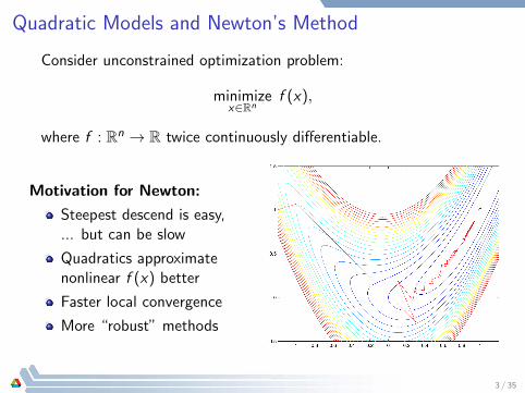
Quadratic Models and Newton’s Method

Consider unconstrained optimization problem:

minimizex∈Rn

f (x),

where f : Rn → R twice continuously differentiable.

Motivation for Newton:

Steepest descend is easy,... but can be slow

Quadratics approximatenonlinear f (x) better

Faster local convergence

More “robust” methods

3 / 35

Quadratic Models and Newton’s Method

minimizex∈Rn

f (x)

Main Idea Behind Newton

Quadratic function approximates a nonlinear f (x) well.

First-order conditions of quadratics are easy to solve.

Consider minimizing a quadratic function (wlog cons t= 0)

minimizex

q(x) =1

2xTHx + bT x

First-order conditions, ∇q(x) = 0, are

Hx = −b

... a linear system of equations

4 / 35

Quadratic Models and Newton’s Method

minimizex∈Rn

f (x)

Newton’s method uses truncated Taylor series:

f (x (k) + d) = f (k) + g (k)T d +1

2dTH(k)d + o(‖d‖2)

where a = o(‖d‖2) means that a‖d‖2 → 0 as ‖d‖2 → 0.

Notation Convention

Functions evaluated at x (k) are identified by superscripts:

f (k) := f (x (k))

g (k) := g(x (k)) := ∇f (x (k))

H(k) := H(x (k)) := ∇2f (x (k))

5 / 35

Quadratic Models and Newton’s Method

minimizex∈Rn

f (x)

Newton’s method defines quadratic approx. at x (k)

q(k)(d) := f (k) + g (k)T d +1

2dTH(k)d ,

and steps to minimum of q(k)(d).

If H(k) positive definite, solve linear system:

mind

q(k)(d) ⇔ ∇q(k)(d) = 0 ⇔ ∇H(k)d = −g (k).

... then sets x (k+1) := x (k) + d

6 / 35

Simple Version of Newton’s Method

minimizex∈Rn

f (x)

Simple Newton Line-Search MethodGiven x (0), set k = 0.repeat

Solve H(k)s(k) := −g(x (k)) for Newton direction

Find step length αk := Armijo(f (x), x (k), s(k))

Set x (k+1) := x (k) + αks(k) and k = k + 1.

until x (k) is (local) optimum;

See Matlab demo

7 / 35

Theory of Newton’s Method

Newton direction is a descend direction if H(k) is positive definite:

Lemma

If H(k) is positive definite, then s(k) from solve ofH(k)s(k) := −g(x (k)) is a descend direction.

Proof.Drop superscripts (k) for simplicityH is positive definite ⇒ H−1 inverse exists and is pos. definite⇒ gT s = gTH−1(−g) < 0⇒ s is a descend direction. �

8 / 35

Theory of Newton’s Method

Newton’s method converges quadratically... steepest descend only linearly

Theorem

f (x) twice continuously differentiable and that H(x) is Lipschitz:

‖H(x)− H(y)‖ ≤ L‖x − y‖

near local minimum x∗.If x (k) sufficiently close x∗, and if H∗ positive definite, thenNewton’s method converges quadratically and αk = 1.

This is a remarkable result:

Near a local solution, we do not need a line search.

Convergence is quadratic ... double the significant digits.

9 / 35

Theory of Newton’s Method

Newton’s method converges quadratically... steepest descend only linearly

Theorem

f (x) twice continuously differentiable and that H(x) is Lipschitz:

‖H(x)− H(y)‖ ≤ L‖x − y‖

near local minimum x∗.If x (k) sufficiently close x∗, and if H∗ positive definite, thenNewton’s method converges quadratically and αk = 1.

This is a remarkable result:

Near a local solution, we do not need a line search.

Convergence is quadratic ... double the significant digits.

9 / 35

Illustrative Example of Newton’s Method

Convergence & failure of Newton: f (x) = x41 + x1x2 + (1 + x2)2

10 / 35

Discussion of Newton’s Method IFull Newton step may fail to reduce f (x), E.g.

minimizex

f (x) = x2 − 1

4x4.

x (0) =√

2/5 creates alternating iterates −√

2/5 and√

2/5.

Remedy: Use a line search.11 / 35

Discussion of Newton’s Method II

Newton’s method solves linear system at every iteration.Can be computationally expensive, if n is large.Remedy: Apply iterative solvers, e.g. conjugate-gradients.

Newton’s method needs first and second derivatives.Finite differences are computationally expensive.Use automatic differentiation (AD) for gradient... Hessian is harder, get efficient Hessian products: H(k)vRemedy: Code efficient gradients, or use AD tools.

12 / 35

Discussion of Newton’s Method III

Problem, if Hessian, H(k) not positive definite

Newton direction may not be definedIf H(k) singular, then H(k)s = −g (k) not well defined:

Either H(k)s = −g (k) has no solution,or H(k)s = −g (k) has infinitely many solutions!

Even if Newton direction exists, it may not reduce f (x)⇒ Newton’s method fails even with line search

13 / 35

Discussion of Newton’s Method IV

Problem, if Hessian, H(k), has indefinite curvature:

Considerminimize

xf (x) = x4

1 + x1x2 + (1 + x2)2

Starting Newton at x (0) = 0, get

x (0) = 0, g (0) =

(02

), H(0) =

0 1

1 2

, ⇒ s(0) =

(−20

)

Line-search from x (0) in direction s(0):

x (0)+αs(0) =

(−2α

0

)⇒ f (x (0)+αs(0)) = (−2α)4+1 = 16α4+1 > 1

for all α > 0, hence cannot decrease f (x) ⇒ α0 = 0

⇒ Newton’s method stalls

14 / 35

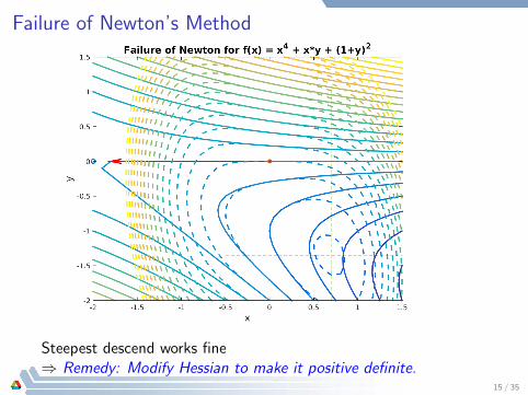
Failure of Newton’s Method

Steepest descend works fine⇒ Remedy: Modify Hessian to make it positive definite.

15 / 35

Modifying the Hessian to Ensure Descend I

Newton’s method can fail, if H(k), is not positive definite.

To modify the Hessian, estimate smallest eigenvalue, λmin(H(k)),

Define modification matrix, Mk :

Mk := max(

0, ε− λmin(H(k)))

I ,

where ε > 0 small, and I ∈ Rn×n identity matrix

Use modified Hessian, H(k) + Mk , which is positive definite

Matlab get smallest eigenvalue: Lmin = min(eig(H))

16 / 35

Modifying the Hessian to Ensure Descend II

Alternative modification

Compute Cholesky factors of H(k):

H(k) + Mk = LkLTk

where Lk lower triangular with positive diagonal

LkLTk is positive definite

Choose Mk = 0 if H(k) is positive definite

Choose Mk not unreasonably large

Related to LkDkLTk factors

... perform modification as we solve the Newton system,

H(k)s(k) := −g(x (k))

17 / 35

Modified Newton Line-Search Method

Given x (0), set k = 0. repeatForm Mk from eigenvalue est. or mod. Cholesky factors.

Get modified Newton direction:(H(k) + Mk

)s(k) := −g(x (k)).

Get step length αk := Armijo(f (x), x (k), s(k)).

Set x (k+1) := x (k) + αks(k) and k = k + 1.until x (k) is (local) optimum;

Modification H(k) − λmin(H(k))I bias towards steepest descend:Let µ = λmin(H(k))−1, then solve

λmin(H(k))(µH(k) + I

)s(k) := −g(x (k)),

As µ→ 0, recover steepest-descend direction, s(k) ' −g(x (k))

18 / 35

Outline

1 Quadratic Models and Newton’s MethodModifying the Hessian to Ensure Descend

2 Quasi-Newton MethodsThe Rank-One Quasi-Newton Update.The BFGS Quasi-Newton Update.Limited-Memory Quasi-Newton Methods

19 / 35

Quasi-Newton Methods

Quasi-Newton Methods avoid pitfalls of Newton’s method:

1 Failure Newton’s, if H(k) not positive definite;

2 Need for second derivatives;

3 Need to solve linear system at every iteration.

Study quasi-Newton and more modern limited-memoryquasi-Newton methods

Overcome computational pitfalls of Newton

Retain fast local convergence (almost)

Quasi-Newton methods work with approx. B(k) ' H(k)−1

⇒ Newton solve becomes matrix-vector product: s(k) = −B(k)g (k)

20 / 35

Quasi-Newton Methods

Choose initial approximation, B(0) = νI Define

γ(k) := g (k+1) − g (k) gradient difference

δ(k) := x (k+1) − x (k) iterate difference,

then, for quadratic q(x) := q0 + gT x + 12xTHx , get

γ(k) = Hδ(k) ⇔ δ(k) = H−1γ(k)

Because B(k) ' H(k)−1, ideally want B(k)γ(k) = δ(k)

Not possible, because need B(k) to compute x (k+1), hence use

Quasi-Newton Condition

B(k+1)γ(k) = δ(k)

21 / 35

Rank-One Quasi-Newton UpdateGoal: Find rank-one update such that B(k+1)γ(k) = δ(k)

Express symmetric rank-one matrix as outer product:

uuT = [u1u; . . . ; unu] , and set B(k+1) = B(k) + auuT .

Choose a ∈ R and u ∈ Rn such that update, B(k+1), satisfies

δ(k) = B(k+1)γ(k) = B(k)γ(k) + auuTγ(k)

... quasi-Newton conditionRewrite Quasi-newton condition as

⇔ δ(k) − B(k)γ(k) = auuTγ(k)

“Solving” last equation of u, then quasi-Newton condition implies

u =(δ(k) − B(k)γ(k)

)/(

auTγ(k))

assuming auTγ(k) 6= 022 / 35

Rank-One Quasi-Newton UpdateFrom previous page: Quasi-Newton condition implies

u =(δ(k) − B(k)γ(k)

)/(

auTγ(k))

assuming auTγ(k) 6= 0

We are looking for update auuT

Assume auTγ(k) 6= 0 (can be monitored)

Choose u = δ(k) − B(k)γ(k)

Given this choice of u, we must set a as

a =1

uTγ(k)=

1(δ(k) − B(k)γ(k)

)Tγ(k)

.

Double check that we satisfy the quasi-Newton condition:

B(k+1)γ(k) = B(k)γ(k) + auuTγ(k)

23 / 35

Rank-One Quasi-Newton Update

Substituting values for a and u we get ...

B(k+1)γ(k) = B(k)γ(k) +

(δ(k) − B(k)γ(k)

) (δ(k) − B(k)γ(k)

)Tγ(k)(

δ(k) − B(k)γ(k))Tγ(k)

= B(k)γ(k) + δ(k) − B(k)γ(k) = δ(k)

Rank-One Quasi-Newton Update

Assuming that (δ − Bγ)T γ 6= we use:

B(k+1) = B +(δ − Bγ) (δ − Bγ)T

(δ − Bγ)T γ.

24 / 35

Properties of Rank-One Quasi-Newton Update

Rank-One Quasi-Newton Update

B(k+1) = B +(δ − Bγ) (δ − Bγ)T

(δ − Bγ)T γ.

Theorem (Quadratic Termination of Rank-One)

If rank-one update is well defined, and δ(1), . . . , δ(n) linearlyindependent, then rank-one method terminates in at most n + 1steps with B(n+1) = H−1 for quadratic with pos. definite Hessian.

Remark (Disadvantages of Rank-One Formula)

1 Does not maintain positive definiteness of B(k)

⇒ steps may not be descend directions

2 Rank-one breaks down, if denominator is zero or small.

25 / 35

BFGS Quasi-Newton Update

BFGS rank-two update ... method of choice

BFGS Quasi-Newton Update

B(k+1) = B −(δγTB + BγδT

δTγ

)+

(1 +

γTBγ

δTγ

)δδT

δTγ.

... works well with low-accuracy line-search

Theorem (BFGS Update is Positive Definite)

If δTγ > 0, then BFGS update remains positive definite.

26 / 35

Picture of BFGS Quasi-Newton Update

We can visualize the BFGS update ...

27 / 35

Picture of BFGS Quasi-Newton Update

We can visualize the BFGS update ...

27 / 35

Convergence of BFGS Updates

Question (Convergence of BFGS with Wolfe Line Search)

Does BFGS converge for nonconvex f (x) with Wolfe line-search?

Wolfe Line-Search Conditions

Wolfe line search finds α:

f (x (k) + αks(k))− f (k) ≤ δαkg (k)T s(k)

g(x (k) + αks(k))T s(k) ≥ σg (k)T s(k).

Unfortunately, the answer is no!

28 / 35

Convergence of BFGS Updates

Question (Convergence of BFGS with Wolfe Line Search)

Does BFGS converge for nonconvex f (x) with Wolfe line-search?

Wolfe Line-Search Conditions

Wolfe line search finds α:

f (x (k) + αks(k))− f (k) ≤ δαkg (k)T s(k)

g(x (k) + αks(k))T s(k) ≥ σg (k)T s(k).

Unfortunately, the answer is no!

28 / 35

Dai [2013] Example of Failure of BFGS

Constructs “perfect 4D example” for BFGS method:

Steps s(k), gradients, g (k), satisfy

s(k) =

[R1 00 τR2

]s(k−1) and g (k) =

[τR1 0

0 R2

]g (k−1),

where τ parameter, and R1,R2 rotation matrices

R1 =

[cosα − sinαsinα cosα

]and R2 =

[cosβ − sinβsinβ cosβ

]Can show that

αk = 1 satisfies Wolfe or Armijo line search

f (x) is polynomial of degree 38 (strongly convex along s(k).

Iterates converge to circle around vertices of octagon... not stationary points.

29 / 35

Limited-Memory Quasi-Newton Methods

Disadvantage of quasi-Newton: Storage & computatn: O(n2)

Quasi-Newton matrices are dense (∃ sparse updates).

Storage & computation of O(n2) prohibitive for large n... solve inverse problems from geology with 1012 unknowns

Limited memory method are clever way to re-write quasi-Newton

Store m� n most recent difference pairs m ' 10

Cost per iteration only O(nm) not O(n2)

30 / 35

Limited-Memory Quasi-Newton Methods

Recall BFGS update:

B(k+1) = B −(δγTB + BγδT

δTγ

)+

(1 +

γTBγ

δTγ

)δδT

δTγ.

= B −(δγTB + BγδT

δTγ

)+

(γTBγ

δTγ

)δδT

δTγ+δδT

δTγ

Rewrite BFGS update as (substitute and prove for yourself!)

B(k+1)BFGS = V T

k BVk + ρkδδT ,

where

ρk =(δTγ

)−1, and Vk = I − ρkγδT .

Recur update back to initial matrix, B(0) � 0

31 / 35

Limited-Memory Quasi-Newton Methods

Idea: Apply m� n quasi-Newton updates at iteration k,corresponding to difference pairs, (δi , γi ) for i = k −m, . . . , k − 1:

B(k) =[V Tk−1 · · ·V T

k−m

]B(0)

[Vk−1 · · ·Vk−m

]+ρk−m

[V Tk−1 · · ·V T

k−m+1

]B(0)

[Vk−1 · · ·Vk−m+1

]+ . . .

+ρk−1δ(k−1)δ(k−1)

T

... can be implemented recursively!

32 / 35

Limited-Memory Quasi-Newton Methods

Recursive procedure to compute BFGS direction, s:

Limited Memory BFGS Search Direction ComputationGiven initial B(0), memory m, set gradient, q = ∇f (x (k)).for i = k − 1, . . . , k −m do

Set αi = ρiδ(i)T γ(i)

Update gradient: q = q − αiγ(i)

end

Apply initial quasi-Newton matrix: r = H(0)qfor i = k − 1, . . . , k −m do

Set β = ρiγ(i)T r

Update direction: r = r + δ(i)(αi − β)end

Return search direction: s(k) := r(= H(k)g (k)

)Cost of recursion is O(4nm) if H(0) is diagonal

33 / 35

General Quasi-Newton Methods

Given any of updates discussed, quasi-Newton algorithm is

General Quasi-Newton (qN) Line-Search MethodGiven x (0), set k = 0.repeat

Get quasi-Newton direction, s(k) = −B(k)g (k)

Step length αk := Armijo(f (x), x (k), s(k))

Set x (k+1) := x (k) + αks(k).

Form γ(k), δ(k), update qN matrix, B(k+1), set k = k + 1.until x (k) is (local) optimum;

34 / 35

Summary: Newton and Quasi-Newton Methods

Methods for unconstrained optimization:

minimizex

f (x)

Quadratic model provides better approx. of f (x)

Newton’s method minimizes quadratic for step d :

minimized

q(k)(d) := f (k) + g (k)T d +1

2dTH(k)d ,

Modify if H(k) not pos. def. (no descend): H(k) + Mk � 0Converges quadratically (near solution)

Quasi-Newton methods avoid need for Hessian H(k)

Update quasi-Newton approx. B(k) ≈ H(k)−1

Limited memory version for large-scale optimization

35 / 35