Embed Size (px)
Citation preview

IMM-NYU 333October 1964
NEW YORK UNIVERSITY
COURANT INSTITUTE OF MATHEMATICAL SCIENCES
ON INVARIANT SURFACES AND BIFURCATION OF PERIODIC
SOLUTIONS OF ORDINARY DIFFERENTIAL EQUATIONS
Robert John Sacker

The corrections below have been performed on the document to follow. The correctionsheet was included with the original publication.
(RJS, 6-2002)
Corrections to IMM-NYU 333
Page Line Reads Should Read
i 11 multiples multipliers7 9 α(ψ) α(µ)7 9 α
′(ψ1) α
′(µ1)
23 6 mapping transformation33 6 < c(r) < 4c(r)44 -4 p p44 -5 P (z, . . .) P (s, . . .)44 15 = 6=45 4 mapping transformation47 11 applying Applying55 2 mapping equation
57 8 e12 ε
12
77 3 cr−1(x, µ) cr−1(x)77 3 Lipr−1(x, µ) Lipr−1(x)
79 7 λ(x, µ) λ(µ)80 7 (all a term) ?
82 7 2β
β2
82 10 1β
β1
83 3 a(x, ) a(x, µ)84 2 |P |s |P |s)86 -2 brackets braces88 2 [ ] [ ]s

ON INVARIANT SURFACES AND BIFURCATION OF PERIODIC
SOLUTIONS OF ORDINARY DIFFERENTIAL EQUATIONSby Robert John Sacker
AbstractWe consider the ordinary differential equation
dx
dt= F (x, µ)
where x is a real n-vector and µ is a real parameter. It is assumed that for all µ in aneighborhood of a critical value µ1 this equation has a periodic solution x = ψ(t, µ) which isasymptotically stable for µ < µ1 (n-1 Floquet multipliers have modulus < 1). As µ increasesthrough µ1 we assume a conjugate pair of multipliers λ(µ) and λ(µ), leaves the unit disccausing ψ to become unstable. It is shown that a two-dimensional asymptotically stableinvariant torus will bifurcate form ψ provided (a) λ(µ1) is not a second, third, or fourth rootof unity, (b) d/dµ|λ(µ1)| > 0, and (c) a certain nonlinear term obtained from F (x, µ) hasthe proper sign (nonlinear damping).
Some cases in which (a) does not hold (resonance cases) are also discussed. In a particularsubcase of the case λ4(µ1) = 1 (but λ and λ2 6= 1), ψ bifurcates into a pair of subharmonicsolutions, exactly one of which is stable. When a single multiplier leaves, λ(µ1) = 1, ψ willin general bifurcate into one stable periodic solution. The case λ3(µ1) = 1 (but λ 6= 1) isdiscussed only by means of a an example in which the instability that develops is so violentcompared to previous cases that there is no stable manifold or periodic solution in a smallneighborhood of ψ.
The existence of the torus is established by two methods. The first is to take an n-1dimensional hyperplane S normal to the orbit ψ and show that the mapping of S into itself,induced by the vector field near ψ, has an invariant curve. In the second method the torus isobtained as the solution of a certain partial differential equation which is basic in the theoryof invariant surfaces.
i

The second main result is concerned with the theory of perturbation of an invariantsurface of a periodic vector field. We consider the differential system
x = f(x, y, µ)y = g(x, y, µ)
where x and y are real vectors, µ is a small real parameter and the functions are periodic inx (e.g., x represents the angular variables on a torus). The problem is to find an invariantmanifold τ(µ) : y = φ(x, µ) whenever τ(0) is known and has certain properties. One ofthe properties assumed by other authors is that the flow (vector field) on τ(0) is parallel,i.e, in appropriate coordinates on the surface, solutions can be obtained from one anotherby a translation. This restriction is dropped since, in general, parallel flow is lost after aperturbation is made. The essential property is the relative strength of the flow against theunperturbed surface and the flow in the surface.
The function φ(x, µ) satisfies the quasilinear partial differential equation∑ν
fν(x, φ, µ)∂φ
∂xν− g(x, φ, µ) = 0
which is solved by an iterative scheme. It is linearized and smoothed so that we have aC∞ equation Lu = h for the approximate solution u. This is made elliptic by addingthe Laplacian, c4u+ Lu = h, c = constant, so that existence and smoothness of a solutionbecomes a matter of quoting well known results. The existence of a solution of the quasilinearequation is obtained from “a-priori” estimates for the solution of the elliptic problem andits derivatives. If the flow against the surface is strong compared to the flow in the surface,then the solution φ(x, µ) will be very smooth since higher derivatives may be estimated.
ii

TABLE OF CONTENTS
Chapter PageI. INTRODUCTION AND SUMMARY 1
Definition of Bifurcation . . . . . . . . . . . . . . . . . . . . . . . . . . 1Statement of Problem and Results . . . . . . . . . . . . . . . . . . . . 3Method of Solution . . . . . . . . . . . . . . . . . . . . . . . . . . . . . 5Notation . . . . . . . . . . . . . . . . . . . . . . . . . . . . . . . . . . . 8
II. BIFURCATION - MAPPING METHOD1. Introduction . . . . . . . . . . . . . . . . . . . . . . . . . . . . . . . . 102. Reduction to a Mapping Problem . . . . . . . . . . . . . . . . . . . 103. Normal Form for the Mapping . . . . . . . . . . . . . . . . . . . . . 11
Definition of “Weight” . . . . . . . . . . . . . . . . . . . . . . . . 13Theorem 1 - Normal Form . . . . . . . . . . . . . . . . . . . . . . 13
4. Existence of Invariant Curve . . . . . . . . . . . . . . . . . . . . . . 15Theorem 2 . . . . . . . . . . . . . . . . . . . . . . . . . . . . . . . 15
5. Solution of Functional Equation . . . . . . . . . . . . . . . . . . . . 19Theorem 3 - Existence (Nonlinear Equation) . . . . . . . . . . . 19Lemma 1 - Existence (Linearized Equation) . . . . . . . . . . . 21Lemma 2 - “A-priori” Estimates . . . . . . . . . . . . . . . . . . 23Lemma 3 - Calculus Inequality . . . . . . . . . . . . . . . . . . . 24
III. BIFURCATION - INVARIANT SURFACE METHOD1. Introduction . . . . . . . . . . . . . . . . . . . . . . . . . . . . . . . . 262. Reduction to Normal Form . . . . . . . . . . . . . . . . . . . . . . . 26
Theorem 4 . . . . . . . . . . . . . . . . . . . . . . . . . . . . . . . 273. Non-resonance Case . . . . . . . . . . . . . . . . . . . . . . . . . . . 30
Theorem 5 . . . . . . . . . . . . . . . . . . . . . . . . . . . . . . . 304. Resonance Case: α(0) = i/4 . . . . . . . . . . . . . . . . . . . . . . 34
Theorem 6. . . . . . . . . . . . . . . . . . . . . . . . . . . . . . . . 345. Another Resonance Case - One Real Exponent . . . . . . . . . . . 39
Theorem 7 . . . . . . . . . . . . . . . . . . . . . . . . . . . . . . . 406. Resonance Case: α(0) = i/3 (an example) . . . . . . . . . . . . . . 41
Violence of Instability . . . . . . . . . . . . . . . . . . . . . . . . . 427. Rate of Growth of Bifurcating Manifold . . . . . . . . . . . . . . . 44
IV. INVARIANT SURFACES1. Introduction . . . . . . . . . . . . . . . . . . . . . . . . . . . . . . . . 462. Notation . . . . . . . . . . . . . . . . . . . . . . . . . . . . . . . . . . 483. Main Theorem . . . . . . . . . . . . . . . . . . . . . . . . . . . . . . 49
Definition of λ . . . . . . . . . . . . . . . . . . . . . . . . . . . . . 49Theorem 8 - Existence (Nonlinear Problem) . . . . . . . . . . . 49
4.“A-priori” Estimates and Solution of Linear Problem . . . . . . . . 53Lemma 4 - “A-priori” Estimates . . . . . . . . . . . . . . . . . . 54Lemma 5 - Existence (Linear Problem) . . . . . . . . . . . . . . 58
5. An Example of Non-parallelizable Flow . . . . . . . . . . . . . . . . 59BIBLIOGRAPHY . . . . . . . . . . . . . . . . . . . . . . . . . . . . . . . . . . . . . . . . . . 61
iii

CHAPTER I
INTRODUCTION AND SUMMARY
In this dissertation we are concerned with the ordinary differential equation
dx
dt= F (x, µ) (1.1)
where x and F are real n-vectors and µ is a real parameter. We will say that (1.1) has
an invariant manifold σk, of dimension k ≤ n, if any solution passing through a point of σk
remains on σk for all time t. The manifold σk is said to be asymptotically stable if all solutions
of (1.1) sufficiently near σk approach σk as t→ +∞, and unstable if in any arbitrarily small
neighborhood N of σk there is at least one solution which leaves N as t→ +∞.
Assume that for µ < µ0, σk is asymptotically stable, but for µ > µ0, it is unstable. One
of the simplest examples of this for n = 2, k = 0, is
z = (i+ µ)z + βz2z
= i[1 + Im β|z|2]z + [µ+Re β|z|2]z(1.2)
where z = x1 + ix2, µ0 = 0 and σ0 = 0. The characteristic exponents for the singular point
z = 0 are α(µ) = i+µ and α. If Re β < 0 (nonlinear damping) then for µ > 0 this equation
has an asymptotically stable limit cycle
|z| =(
µ
−Re β
) 12
i.e., a stable invariant manifold σ1(µ) with σ1(0) = σ0, which branches off or bifurcates form
σ0 as µ increases through zero (Fig. 1).
Definition: We say that the manifold σ` bifurcates* from σk as µ increases through µ0 if
σ`(µ0) = σk but σ`(µ) and σk have no points in common for µ > µ0.
The above example illustrates a general result obtained by E. Hopf [2] which may be
stated in a somewhat weaker form as follows. Assume (1.1) is analytic and has a stationary
solution x = 0 for |µ| sufficiently small. Assume that for µ < 0 all the characteristic
exponents a(µ) satisfy Re a(µ) < 0. As µ increases through zero assume a conjugate pair
of exponents α(µ), α(µ) 6= 0 crosses the imaginary axis and enters the right half plane
with Re α(0) = 0, Re α′(0) > 0, while the remaining exponents satisfy Re α(µ) ≤ a0 for
some constant a0 < 0. Then if a certain constant depending on terms of degree ≤ 3 in the
expansion of F about x = 0 has the proper sign (nonlinear damping), then the solution
*See Minorsky [1] for a discussion of bifurcation.
1

2

σ0 : x = 0 bifurcates into an asymptotically stable* periodic solution σ1(µ) : x = ψ(t, µ)
for µ > 0 sufficiently small. ψ(t, 0) = 0 and ψ(t, µ) 6= 0 for µ > 0. If the constant has the
opposite sign, then ψ will exist in advance (µ < 0) but will be unstable, i.e, as µ decreases
through zero the unstable origin σ0 becomes stable and bifurcates into an unstable periodic
solution. Hopf assumed analyticity of the functions and used power series expansions in his
proof- the method of Poincare.
In this dissertation we consider the case in which ψ(t, µ) becomes unstable as µ increases
further and passes through a second critical point µ1, and a pair of Floquet exponents
α(µ), α(µ) enters the right half plane Re ς > 0 with Re α′(µ1) > 0, i.e., a pair of Floquet
multipliers λ(µ), λ(µ) leaves the unit disc |ς| ≤ 1 with d/dµ|λ(µ1)| > 0.
The Floquet exponents are associated with (1.1) linearized along ψ(t, µ),
y = Fx(ψ(t, µ), µ)y (1.3)µ
If the frequency of ψ1 ≡ ψ(t, µ1) is ω1 then Im α(µ1) ≡ ω2 (determined only up to integral
multiples of ω1) is the frequency of oscillation about ψ1 of solutions of (1.3)µ1 starting near
ψ1. Floquet theory asserts that (1.3)µ1 has a family of solutions of the form
φ(t) = A(t) cosω2t+B(t) sinω2t
where A and B have frequency ω1. If ω2/ω1 is irrational (non-resonance case) then φ(t) is
not periodic. If ω2/ω1 = rational = p/q in lowest form (resonance case) then φ(t) is periodic
and has frequency ω1/q, i.e., the period P = qP1 (P1 = 2π/ω1 is the period of ψ1). If q > 1
we call φ(t) a subharmonic solution. In terms of the Floquet multiplier λ(µ1) = ei2π
ω2ω1 ,
non-resonance is characterized by λq(µ1) 6= 1 for any integer q and resonance by λq(µ1) = 1
for some integer q.
Throughout this work we will assume that F has ρ ≥ 5 continuous derivatives with
respect to x and µ in some neighborhood of ψ(t, µ). We will prove the following.
Statement 1: If certain low order resonances are avoided, specifically, if
(a) ω2/ω1 6= p/q in lowest form with q = 1, 2, 3, 4 i.e., if λq(µ1) 6= 1 for those q, and if
(b) Re α′(µ1) > 0 and
(c) a certain constant obtained from the terms of degree ≤ 3 in the expansion of F about
ψ(t, µ1) has the proper sign, then ψ(t, µ) bifurcates into a unique asymptotically stable torus
σ2(µ) as µ increases through µ1. For r an integer, 0 ≤ r ≤ ρ− 1, σ2(µ) exists as an r-times
continuously differentiable manifold for 0 < µ−µ1 < δr where δr depends on r, the terms of
*i.e., n− 1 of the Floquet exponents associated with ψ(t, µ) have negative real parts.
3

degree ≤ 3 mentioned in (c), and M0 = |F |r*. In general δr → 0 as r →∞. If the constant
in (c) has the opposite sign, then the torus σ2 exists in advance (µ < µ1) and is unstable.
A model of such bifurcation phenomenon was given by E. Hopf [3]. Hence we show
essentially that for the second bifurcation (i.e., periodic solution into torus) Hopf’s model is
the generic situation.
It is worth noting that even if F (x, µ) is analytic, this torus may not be analytic but only
represented by functions with finitely many derivatives. Thus any method based on power
series expansions must fail.
Three resonance cases are discussed and we prove the following.
Statement 2: If
(a) ω2/ω1 = 1/4, i.e., λ4(µ1) = 1
(b) Re α′(µ1) > 0 and
(c) certain conditions are satisfied by the terms of degree ≤ 3 in the expansion of F
about ψ(t, µ1), then as µ increases through µ1, ψ(t, µ) bifurcates into a pair of subharmonic
solutions**. One solution is asymptotically stable and the other is unstable.
The next result deals with the case in which one real Floquet exponent α(µ) becomes
positive.
Statement 3: If
(a) α(µ1) = 0, α(µ) real, (b) α′(µ1) > 0 and
(c) a certain constant obtained from the terms of degree ≤ 2 in the expansion of F about
ψ(t, µ1) is not zero, then as µ increases through µ1, ψ(t, µ) bifurcates into an asymptotically
stable periodic solution having the same period.**
The third resonance case, ω2/ω1 = 1/3, is discussed by means of an example which
illustrates the violent instability which develops after bifurcation.
The resonances (Statements 2 and 3 and the example) are treated in Chapter III where
the rate of growth of the bifurcating manifolds is also discussed. The proofs of Statements 2
and 3 require the usual construction of periodic solutions by means of the implicit function
theorem [4]. In contrast, Statement 1 requires the construction of a 2-dimensional surface
and thus different techniques are needed. Statement 1 is proved in Chapter II and again in
Chapter III. In Chapter II the problem is treated by working with the mapping induced by
*This norm is defined at the end of the chapter. The differentiation is with respect to x and µ and the
supremum is taken over a small neighborhood of ψ(t, u).** The deviation of period with µ is eliminated by introducing a new parameter s in place of t.
4

the vector field near ψ, the so-called “method of surfaces of section” of Poincare and G.D.
Birkhoff. The method is described in detail in the introduction to that chapter.
In Chapter III we treat the differential equation directly. The torus is obtained as the
solution of a certain partial differential equation which arises in the theory of perturbation
of an invariant surface of a periodic vector field. This theory, treated in Chapter IV, is
concerned with the problem of finding an invariant manifold τ(µ) of
x = f(x, y, µ)y = g(x, y, µ)
(1.4)
whenever τ(0) is known and has certain properties. µ is a small parameter, x and y are
vectors, and the functions are periodic in x. If τ(0) is the surface φ0(x), then the problem is
to find a solution τ(µ) : y = φ(x, µ) of the quasilinear partial differential equation∑ν
fν(x, φ, µ)∂φ
∂xν− g(x, φ, µ) = 0 (1.5)
with φ(x, 0) = φ0(x). The properties of the flow (vector field) in the surface τ(0) and the
flow against* the surface are essential in determining the existence and smoothness of the
perturbed surface. We say that the flow in τ(0) is parallel if x = constant on the surface.
The flow is parallelizable if it is parallel in appropriate coordinates on the surface. The case
of parallel flow has received much attention (Diliberto [5, 6], Bogoliubov and Mitropolski [7,
8], Hale [9, 10], Diliberto and Hufford [11]).
In treating the general problem of perturbation of invariant surfaces the assumption of
parallel flow is much too stringent and unnatural since it is generally lost after the perturba-
tion is made. When the unperturbed surface contains lower dimensional invariant manifolds
(e.g., stationary points) it is usually impossible to parallelize the flow. The characteristics on
the surface may form envelopes and it seems unsatisfactory to use methods such as those of
Bogoliubov and Mitropolski [7] in which (1.5) is solved by integrating along characteristics.
The characteristics method is associated with initial value problems whereas the problem
of solving (1.5) defined on a torus may be formulated more naturally as a boundary value
problem in which the boundary condition to be imposed is the periodicity of the solution
in x. It is the latter formulation which is considered in Chapter IV. The solution of (1.5)
is obtained by an iterative process. At each stage the equation is linearized and smoothed
so that we obtain an equation Lu = h where h and the coefficients in L are C∞ functions.
This is then modified to give an elliptic equation
c4u+ Lu = h
*We do not consider the case in which the flow is away from τ(0).
5

where c = c(n) is a constant which tends to zero as n, the number of iterations, tends to ∞and 4 is the Laplacian. Under the given conditions we obtain existence and C∞ smoothness
of a solution of the above equation. The existence of the solution of the nonlinear equation
then follows from the “a priori” estimates for the solution of the linear equation and its
derivatives. In deriving these estimates there are two parameters, β > 0 and λ ≤ 0, which
play a fundamental role. β is a measure of the flow against the unperturbed surface and λ
is a measure of the flow in the surface. It is shown that if β + rλ > 0, r and integer ≥ 2,
and another condition* is satisfied, then for sufficiently small µ the perturbed surface τ(µ)
has r − 1 Lipschitz continuous derivatives. This is the second main result established in
this dissertation (Theorem 8). It says essentially that if the flow against the surface is great
(β large) compared to the flow in surface, then the perturbed surface will be very smooth.
Heuristically we can see the need for such an assumption. For consider (in one x dimension)
two characteristics C1 and C2 approaching the equilibrium x = 0, (see Figs. 2 and 3 where
τ(0) is the line y ≡ 0). If as in Fig. 2, the flow against y ≡ 0 is small compared to the flow
in y ≡ 0 (shown by arrows), then a cusp may develop. McCarthy [13] and Kyner [14] discuss
an example of such a situation. If the relative strength of these flows is reversed (Fig. 3)
then C1 and C2 tend to meet in a smooth fashion.
Thus even if f and g are C∞ functions and τ(0) is a C∞ surface it may happen that τ(µ)
has only finitely many derivatives. In fact, in the example of Kyner the perturbed surface
has a cusp for arbitrarily small µ > 0.
The result of Kyner [14] is not restricted to parallel flow. In the case of non-parallelizable
flow he postulates the invertibility of a certain linear transformation and obtains a perturbed
surface which is Lipschitz continuous. Higher derivatives are not treated.
In the special case in which the flow on τ(0) is parallel, λ = 0 and thus τ(µ) will have
any finite number of continuous derivatives provided µ is sufficiently small. Such is the case
if we consider the equation
ξ = F (ξ) + µF ∗(ξ, t, µ) (1.6)
(ξ an n-vector) where the functions are C∞ in all arguments and have period T in t. It is
assumed that for µ = 0 there is a limit cycle Γ which is asymptotically stable (n− 1 of the
characteristic exponents of the linear variational equation have negative real parts). τ(0) is
then the torus Γ× {0 ≤ t ≤ T} with the faces t = 0 and t = T identified (see Fig. 4). It is
known ([15], [8], [9], [11]) that coordinates can be introduced such that the flow on τ(0) is
parallel. Hale [9] and Diliberto and Hufford [11] treat (1.6) in the degenerate case in which
*This condition (number 3 in Theorem 8) is used to solve the linearized equation and is precisely the
“positive” condition of Friedrichs [12].
6

7

the flow against τ(0) vanishes for µ = 0 (some of the characteristic exponents have zero
real part for µ = 0). It is this case which arises in the bifurcation problem in Chapter III
(see equation 3.24) and thus the results of these authors could have been applied at this
stage to prove existence of the torus. The theory of Chapter IV also takes this degeneracy
into account and may be considered as a new derivation of the results of the above authors.
Its chief advantage, however, lies in its applications to cases of non-parallelizable flow. (see
example in Chapter IV).
Notation: We now introduce some notation which will be used throughout the rest of
our work. For r a positive integer
F (x, y, µ) ∈ Cr(x, y) ∩ C(µ)
means that F has r derivatives with respect to x and y which are continuous in (x, y, µ).
F (x, y, µ) ∈ Cr(x, y) ∩ Lipr(x, y) ∩ C(µ)
means the same as above and the derivatives are Lipschitz continuous in x and y uniformly
in µ.
For a vector f = (fi) define
|f | =
(∑i
f 2i
) 12
= (f, f)12
We will consider functions f(x, µ) defined for x a vector in some domain G and µ a small
parameter. For r ≥ 0 an integer define the norm
|f |r = max0≤ρ≤r
supx∈G|Dρf |
where Dρ is any ρth order derivative of f with respect to the components xi of x. Unless
otherwise stated, differentiation will never be performed with respect to µ.
For two real vectors u = (u1, . . . , un) and v = (v1, . . . , vn), the symbol (u, v) will denote
the usual inner product
(u, v) =n∑k=1
ukvk.
8

9

CHAPTER II
BIFURCATION - MAPPING METHOD
1. Introduction
In this chapter we treat the bifurcation problem by considering the mapping induced
by the vector field near the periodic solution: the method of surfaces of section mentioned
earlier.
We consider the differential equation
dx
dt= F (x, µ) (2.1)
where x and F are real n-vectors and µ is a real parameter. Suppose that for all sufficiently
small µ, |µ| < µ∗, (2.1) has a periodic solution x = ψ(t, µ) with period 2π. Assume that F
has ρ ≥ 5 continuous derivatives with respect to x and µ in some neighborhood of ψ and
that in this neighborhood
|F |ρ ≤M0
where differentiation is with respect to x and µ.
Suppose that ψ is asymptotically stable for µ < 0 in the sense that n-1 of the Floquet
multipliers lie inside the unit circle in the complex plane. As µ increases through zero we
assume that a conjugate pair of the multipliers
λ(µ) = e2πα(µ), λ(µ) = e2πα(µ)
leaves the unit circle with
Re α(0) = 0, Re α′(0) > 0
while the remaining n-3 stay inside. Hence the periodic solution ψ becomes unstable.
We do not require that ψ is obtained by a bifurcation from an equilibrium as discussed
in Chapter I but just consider any periodic solution which loses its stability in the above
manner as µ passes through a critical value (assumed to be µ = 0).
2. Reduction to a Mapping Problem
We now obtain the mapping described by the flow near the periodic solution ψ. Let C
be the curve described by ψ. Choose a point P on C and let S be the n-1 dimensional
hyperplane normal to C at P . Let P be the origin of coordinates x = (x(1), . . . , x(n−1))
describing S. It is known [16; p.50] that any solution of (2.1) starting on S and close enough
to P will return to S for the first time after a time lapse of 2π+ ε(x) where ε→ 0 as x→ 0.
In a small neighborhood of P this defines a mapping T of S into itself having P as a fixed
point
T : x1 = Dx+ . . . (2.2)
10

It is known [16; p.163] that the eigenvalues of D are just the n − 1 previously mentioned
Floquet multipliers. Thus for µ < 0, P is an asymptotically stable fixed point which becomes
unstable as µ increases through zero.
The existence of a torus will be established by showing that P bifurcates into a closed
curve C, lying in S which is invariant under T , i.e., if q is a point of C, then Tq = q1 is on
C (see Fig. 5).
3. Normal Form for the Mapping
By appropriately transforming coordinates we will put the mapping in a certain normal
form which is needed in the existence theorem. We assume that a real linear transformation
of coordinates has been carried out so that D is in the real form
D =
Re λ(µ) −Im λ(µ)
0Im λ(µ) Re λ(µ)
0 S(µ)
where S(µ) is a matrix whose eigenvalues σ(µ) satisfy
|σ(0)| < 1 (2.3)
and
sup|Y |=1
|S(0)Y | = σ0 < 1
where Y = Col(x(3), . . . , x(n−1)) and |Y | is the ordinary Euclidean length of a vector (Y, Y )12 .
Let z = x(1) + ix(2). Then in the z, Y coordinates the mapping is
z1 = λ(µ)z + U(z, z, Y, µ)T :
Y1 = S(µ)Y + V (z, z, Y, µ)(2.4)
where U is complex and V is real. The functions U, V, λ and S have five continuous derivatives
in a neighborhood of (z, Y, µ) = 0 which we assume to be
|z|2 + |Y |2 ≤ 2, |µ| < µ∗.
We assume U and V to be expanded into Taylor series up to polynomials of degree 4 plus
remainder.
In order to motivate the following theorem consider the following example of a mapping
z1 = ei+µ+β|z|2z
Y1 = SY + b|z|2
11

12

where β is complex, b is a real constant vector and S is a matrix which satisfies (2.3). If
Re β < 0, this mapping has the invariant curve
|z| =(
µ
−Re β
) 12
, Y = (S − I)−1bµ
−Re β
contained in a neighborhood |z| ≤ c√µ, |Y | ≤ c2µ, c a constant. We now consider the effect
of perturbing this example by adding more nonlinear terms. In such an oblate neighborhood
Y is small of order µ whereas z is small only to order µ12 . More precisely consider the
neighborhood
N : z = aζ, Y = a2Y
where |ζ|2 + |Y |2 ≤ 2 and a is a small parameter, 0 ≤ a ≤ 1. In N the monomial Mτ =
Y p(i)z
qzr, τ = 2p + q + r, satisfies |Mτ |k ≤ c(k)aτ where differentiation is with respect to
Y(i), ζ, and ζ and c(k) is a constant depending only on k.
Definition. We call τ the weight of Mτ . In the following theorem we will transform the
mapping (2.4) into a form similar to the above example in which monomials of weight 2 and
3 will serve to determine the invariant curve in the first approximation while the remaining
terms will act as small perturbations. The transformations used are of the type treated by
B. Segre [17]. See also A. Kelly [18] for an excellent bibliography.
Theorem 1. If λ4(0) 6= 1, λ3(0) 6= 1 and (2.3) is satisfied, then there exists a µ0 ≤ µ∗
such that for |µ| < µ0 there exists a transformation
z = cw + P (w, w,W, c, µ)0 < c ≤ 1
Y = cW + P (w, w,W, c, µ)
with P and P polynomials in w, w, and W , which carries (2.4) into the form
w1 = e2πα(µ)+c2β(µ)|w|2w +R4(w, w,W, c, µ)
W1 = S(µ)W +R3(w, w,W,C, µ)(2.5)
where Rk are function whose Taylor expansions* about (w, w,W ) = 0 contain no terms
of weight < k. P and P contain no constant or linear terms. For proper choice of c the
transformation is one-to-one in the neighborhood |w|2 + |W |2 ≤ 2.
Proof: In this proof subscripts on functions will carry the same significance as for Rk
defined above. We write the first equation of (2.4) as
z1 = λ(µ)z + u(z, z, µ) + v(z, z, Y, µ) + F4 (2.6)
*By the smoothness assumption made after (2.4), Rk is well defined provided k ≤ 4.
13

where u contains quadratic and third order terms in z and z and v = Y ′[p(µ)z+ q(µ)z] with
p, q vectors and prime denoting transpose. We transform (2.6) by
z = w + r(µ)wkw`, k + ` = 2, 3 (2.7)
to obtain
w1 = λ(µ)w + u(w, w, µ)− g(µ)wkw` + v(w, w, Y, µ) + F4
where
g(µ) = (λkλ` − λ)r(µ), λ = λ(µ)
Unless k = 2, l = 1 we see that r(µ) may be determined so that (2.7) removes the term
wkw` from u. By successive applications of (2.7), we obtain the form
w1 = λ(µ)w + b(µ)|w|2w + v(w, w, Y, µ) +G4. (2.8)
The transformation
w = ζ + Y ′r(µ)ζkζ`, k + ` = 1 (2.9)
with r(µ) a vector carries (2.8) into
ζ1 = λ(µ)ζ + b(µ)|ζ|2ζ + v(ζ, ζ, Y, µ)− Y ′g(µ)ζkζ` + G4
where
g(µ) = [S ′(µ)λkλ` − λI]r(µ), λ = λ(µ)
and I is the identity matrix. Since λ(0) is on the unit circle and from (2.3) the eigenvalues
of S ′(0) are inside the unit circle, we see that r(µ) may be determined for µ sufficiently small
such that the term ζkζ` is removed from v. The mapping now has the form
ζ1 = λ(µ)ζ + b(µ)|ζ|2ζ +H4. (2.10)
The second equation of (2.4) may be written
Y1 = S(µ)Y + s(ζ, ζ, µ) +H3 (2.11)
where s is quadratic in ζ and ζ. The transformation
Y = X + r(µ)ζkζ`, k + ` = 2
reduces (2.11) to
X1 = S(µ)X + s(ζ, ζ, µ)− g(µ)ζkζ` + H3
where
g(µ) = [λkλ`I − S(µ)]r(µ), λ = λ(µ).
14

Just as before r(µ) may be determined for µ sufficiently small. Thus the mapping has the
form (2.10) together with
X1 = S(µ)X + V3.
Using λ(µ) = e2πα(µ), (2.10) may be written
ζ1 = e2πα(µ)[1 + β(µ)|ζ|2]ζ +H4
= e2πα(µ)+β(µ)|ζ|2ζ + H4
with β = b/λ. All the previous transformations may be combined into one; z = ζ + . . . , Y =
X + . . . where the dots represent polynomials in ζ, ζ, X without constant and linear terms.
It is one-to-one in a neighborhood |ζ|2 + |X|2 ≤ 2c. The transformation ζ = cw, X = cW
then gives the desired results.
4. Existence of an Invariant Curve
Having the mapping in the form (2.5) we may now establish the existence of an invariant
curve and hence, according to the discussion of Section 2, an invariant torus of the differential
equation (2.1).
Theorem 2. In (2.4) assume
1. λ4(0) 6= 1, λ3(0) 6= 1 (non-resonance)
2. λ(µ), S(µ), U, V ∈ C`(z, z, Y, µ) for ` an integer ≥ 5, |µ| ≤ µ∗, |z|2 + |Y |2 ≤ 2 and
assume S(µ) satisfies (2.3).
In (2.5) assume
3. A = 2πRe α′(0) > 0, B = Re β(0) < 0.
Let r, 1 ≤ r ≤ ` be a positive integer. Then there exists µr ≤ µ∗ such that for 0 ≤ µ < µr,
(2.4) has an asymptotically stable invariant curve
z = a0√µeiθ + µf(θ, µ)eiθ
Y = µg(θ, µ)(2.12)
where a0 =√−A/B . f and g are defined for all θ and 0 < µ < µr, have period 2π in θ,
f, g ∈ Cr−1(θ) ∩ Lipr−1(θ) ∩ C(µ)
and
|f |r−1, |g|r−1 ≤ c(r)
15

where c(r) is a constant which depends only on r and differentiation is with respect to θ
only. In general µr → 0 as r increases. µr depends on the coefficients of terms of degree ≤ 3
in(2.4), i.e., on terms of degree ≤ 3 in the expansion of (2.1) about ψ. µr also depends on
the constant M0 defined after (2.1).
Proof. In (2.5) we assume c to be fixed such that the mapping is one-to-one for |w|2 +
|W |2 ≤ 2. Note that c depends only on the coefficients of terms of degree ≤ 3 in (2.5).
We restrict attention to a neighborhood w = az,
W = a2Y (2.13)
where |z|2 + |Y |2 ≤ 2 and 0 ≤ a ≤ 1. Then (2.5) becomes
z1 = e2πα(µ)+a2c2β(µ)|z|2z + f1(z, z, Y, a, µ)
Y1 = S(µ)Y + f2(z, z, Y, a, µ)
and
|f1|r ≤ c(r)a3, |f2|r ≤ c(r)a
where differentiation is with respect to z, z and Y . Note that the subscripts on the functions
are used simply for identification and have nothing to do with “weight” as they did in the
previous theorem.
Expanding α, β, and S, we obtain
z1 = exp[2πα(0) + µ2πα′(0) + a2c2β(0)|z|2]z + f3(z, z, Y, a, µ)
Y1 = S(0)Y + f4(z, z, Y, a, µ)
where
|f3|r ≤ c(r)(µ2 + a2µ+ a3), |f4|r ≤ c(r)(a+ µ).
LettingS(0) = S, 2πα(0) = iτ
2πα′(0) = A+ iA, β(0) = B + iB
and choosing
a =
√−Aµc2B
, 0 ≤ µ < µ0 = min
(µ∗,
c2B
−A
)we obtain
z1 = exp[i(τ + µφ) + µA(1− |z|2)]z + f5(z, z, Y, µ)
Y1 = SY + f6(z, z, Y, µ)(2.14)
where
φ = A− AB
B|z|2
16

and
|f5|r ≤ c(r)µ32 , |f6|r ≤ c(r)µ
12 .
The unperturbed mapping (f5, f6 ≡ 0) has an invariant curve |z| = 1, Y ≡ 0. We
introduce coordinates in a small toriod (see Fig. 6) surrounding this curve.
z = (1 + ρ)eiθ, |ρ|2 + |Y |2 ≤ 1
4. (2.15)
The first equation of (2.14) becomes
ρ1 = (1− 2µA)ρ− 3µAρ2 − µAρ3 + f7(ρ, θ, Y, µ)
θ1 = θ + τ + µ
[A− AB
B(1 + ρ)2
]+ f8(ρ, θ, Y, µ)
where
|f7|r, |f8|r ≤ c(r)µ3
2.
Letting ρ = µ12u, Y = µ
12v, we finally obtain (2.16)
u1 = (1− 2µA)u + µ[g(θ) + G(θ, u, v, µ)]
θ1 = θ + τ + µ[f0 + F (θ, u, v, µ)]
v1 = Sv + h(θ) + H(θ, u, v, µ)
(2.17)
where f0 is a constant, all functions have period 2π in θ and
|g|r, |h|r ≤ c(r); |G|r, |H|r, |F |r ≤ c(r,K)µ12 (2.18)
for
|u|2 + |v|2 ≤ K2, 0 ≤ µ ≤ 1
4K2
where differentiation is with respect to all variables except µ. c and c are constants which
depend only on the arguments shown. See Fig. 7 for a description of the toroidal neighbor-
hood in the W, w coordinates. Finding an invariant curve u = u(θ, µ), v = v(θ, µ) of (2.17)
is equivalent to solving the functional equation
u(θ1)− (1− 2µA)u(θ) = µG(θ, u, v, µ)
v(θ1)− Sv(θ) = H(θ, u, v, µ)
θ1 = θ + τ + µF (θ, u, v, µ)
(2.19)
17

18

where F = f0+F , f0 a constant, G = g(θ)+G and H = h(θ)+H satisfy (2.18). Theorem
3 which follows guarantees the existence of a unique solution u = u(θ, µ), v = v(θ, µ) of (2.19)
satisfying all our requirements. The form (2.12) is obtained by applying the transformations
(2.16), (2.15), (2.13) and finally, the transformation of Theorem 1.
We now prove the stability of the invariant curve. If u(θ, µ), v(θ, µ) is the solution of
(2.19) for 0 < µ < µr, let u = u(θ, µ) + δu, v = v(θ, µ) + δv in (2.17) to obtain the nonlinear
variational mapping
δu1 = (1− 2µA)δu+ µ(Gu − u′Fu)δu+ µ(Gv − u′Fv)δv
δv1 = Sδv + (Hu − µv′Fu)δu+ (Hv − µv′Fv)δv
where prime is d/dθ and Fu etc. are evaluated at u(θ, µ)+εδu, v(θ, µ)+εδv, 0 < ε < 1. From
(2.18) we see that the derivatives of F,G, and H with respect to u and v are ≤ (constant)
µ12 uniformly in a small tube R : |δu|2 + |δv|2 ≤ constant. Hence in R for µ sufficiently
small, 0 < µ < µr ≤ µr, the above mapping is a contraction. This completes the proof of
the theorem.
5. Solution of Functional Equation
The above stability argument is based on the principle of contraction, i.e., the eigenvalues
of the linear part of the mapping are less than unity in modulus. This same principle will
now be utilized to prove existence of a solution of equation (2.19).
Theorem 3. In (2.19) assume
1. A > 0, |Sv| ≤ σ0|v|, 0 < σ0 < 1 σ0 constant
2. F,G,H ∈ Cr(θ, u, v) ∩ C(µ), r ≥ 1,
for 0 ≤ µ < µ0 and |u|2 + |v|2 ≤ K2, K sufficiently large and assume these functions
satisfy (2.18) and have period 2π in θ.
Then there exists µr ≤ µ0 such that for 0 < µ < µr (2.19) has a unique solution
u(θ, µ), v(θ, µ) having period 2π in θ.
u, v ∈ Cr−1(θ) ∩ Lipr−1(θ) ∩ c(µ)
and |u|r−1, |v|r−1 ≤ K uniformly in µ where differentiation is with respect to θ only. µr
depends on A, σ0, r and the constants c and c in (2.18). In general, µr → 0 as r increases.
Proof. Define b = min(2A, 1− σ0). Then 0 < b < 1. Also define
K = b−r−1c0(r) c(r)2δ(r+1)+3
19

where c0(r) and δ are defined in Lemma 2 and c(r) comes from (2.18). We will construct
successive approximations un and vn with u0 ≡ 0, v0 ≡ 0. For convenience let wn =(unvn
).
As an induction assumption suppose wn−1 satisfies
wn−1 ∈ Cr(θ) ∩ C(µ), 0 < µ < µ0. (2.20)
|wn−1|r < K (2.21)
Inserting this approximation in (2.19) we obtain
u(θ1) − (1− 2µA)u(θ) = µGn(θ, µ)
v(θ1) − Sv(θ) = Hn(θ, µ)(2.22)
θ1 = θ + τ + µFn(θ, µ)
to be solved for wn(θ, µ), where
Fn(θ, µ) = F (θ, wn−1(θ, µ), µ) (2.23)
and so on. We now verify the conditions of Lemma 1.* We have Fn, Gn, Hn ∈ Cr(θ) ∩ C(µ)
for 0 < µ < µ′0 = min(µ0, 1/4K2). Also if we define m = infθ,µ Fnθ we have, using (2.18),
b + rm ≥ b− crµ 12 > b/2 for µ small, 0 < µ < µ′ ≤ µ′0, where c depends on K and c(r,K).
Unless F ≡ 0 we see that µ′ → 0 as r increases. By Lemma 1,∗ (2.22) has a solution wn(θ, µ)
which satisfies (2.20) for 0 < µ < µ′′ ≤ µ′. To verify (2.21) for wn define Qn =
(GnHn
)and
apply Lemma 2∗.
|wn|r ≤c0(r)|Qn|r[1 + |Fnθ |r−1]δ(r)
(b+ rm)r+1.
From (2.18) we have
|Fnθ |r−1 ≤ c1µ12 < 1
|Qn|r ≤ 2c(r) + c1µ12 < 4c(r)
for µ small, 0 < µ < µ < µ′′. Thus
|wn|r < (2/b)r+14c(r)c0(r)2δ(r) = K.
Repeating this procedure we generate a sequence {wn} which satisfies (2.20) and (2.21) for
0 < µ < µ.
To show convergence define δun+1(θ) = un+1(θ, µ)− un(θ, µ), δGn+1 = Gn+1−Gn and so
on. Then from (2.22)
δun+1(θ1)− (1− 2µA)δn+1u(θ) = µ[δGn+1 − u′nδFn+1]
δvn+1(θ1)− Sδvn+1(θ) = δHn+1 − v′nδFn+1.
*This lemma is proved later.
20

θ1 = θ + τ + µFn+1(θ, µ)
Defining Qn as before, we have from the first estimate of Lemma 2
|δwn+1|0 ≤2
b{|Qn+1|0 + |wn|1 |δFn+1|0}.
Using (2.21), (2.23) and (2.18) we have
|δwn+1|0 ≤ cµ12 |δwn|0 ≤
1
2|δwn|0
for µ sufficiently small, 0 < µ < µ ≤ µ, i.e., uniform convergence of the wn. For the θ
derivative w(λ)n 0 ≤ λ ≤ r−1 we have from Lemma 3 (with m = 1, x1 = θ, ` = r) and (2.21)
|w(λ)n+p − w(λ)
n |0 ≤ 2K c(λ, r)|wn+p − wn|1−(x/r)0 .
Hence {wn} converges to a solution w of (2.19) and w(θ, µ) ∈ Cr−1(θ)∩C(µ). The Lipschitz
condition follows from passing to the limit in
|w(λ)n (θ′, µ)− w(λ)
n (θ, µ)| ≤ |wn|λ+1|θ′ − θ| ≤ K|θ′ − θ|.
Uniqueness follows by applying the convergence argument to the sequence {w1, w2, w1, w2, . . .}where w1 and w2 are two supposed solutions. Finally we note that |w|r−1 ≤ K. Thus the
theorem is proved with µr = µ.
Lemma 1. (Solution of Linear Functional Equation)
Consider the equation
u(θ1) − (1− 2µA)u(θ) = µG(θ)
v(θ1) − Sv(θ) = H(θ)(2.25)
θ1 = θ + τ + µF (θ, µ) (2.26)
where τ is constant, 0 < µ < µ′, A > 0 and |Sv| ≤ σ0|v| for some σ0, 0 < σ0 < 1. Define
b = min(2A, 1− σ0) and m = infθ,µ Fθ. Assume
1. b+ rm > 0 for some integer r ≥ 0
2. F,G,H ∈ Cr(θ) ∩ C(µ) and have period 2π in θ.
Then for
0 < µ < µ′′
= min
[1
2A,
1
|m|, µ′, 1
](2.25-6) has a solution u(θ, µ), v(θ, µ) ∈ Cr(θ) ∩ c(µ) having period 2π in θ.
Remark. Since F is periodic in θ, m will be ≤ 0 and hence if 1 is true for some integer
r = r0 then it is true for any smaller integer r < r0.
21

Proof. Each equation has the form
Y (θ1)−D(µ)Y (θ) = P (θ, µ) (2.27)
with
|D(µ)Y | ≤ (1− µb)|Y | (2.28)
where D(µ) represents either S(µ) or 1−2µA. Let I be any closed subinterval of (0, µ′′). We
may solve (2.26) for the negative iterates θ−1, θ−2, . . . where θ−n+1 = θ−n + τ + µF (θ−n, µ)
since ∣∣∣∣dθ1
dθ
∣∣∣∣ ≥ 1 + µm > 0 for µ ∈ I.
We allow D to depend on θ also and write
Y (θ)−D(θ−1, µ)Y (θ−1) = P (θ−1, µ)
D(θ−1, µ)Y (θ−1)−D(θ−1, µ)D(θ−2, µ)Y (θ−2) = D(θ−1, µ)P (θ−2, µ)...
Adding and passing to the limit
Y (θ, µ) =∞∑j=1
j−1∏k=1
D(θ−k, µ)P (θ−j, µ)
where∏0
k=1 ≡ 1. From (2.28) we see that the series converges uniformly for all θ and for
µ ∈ I. If r = 0 we are finished. If r = 1 we differentiate term by term using
d
dθθ−j =
dθ−jdθ−j+1
. . .dθ−1
dθ
and ∣∣∣∣ ddθθ−j∣∣∣∣ ≤ ( 1
1 + µFθ
)j.
The differentiated series converges uniformly for the same values of θ and µ since for |y| = 1,
|D(µ)y|1 + µFθ
≤ 1− µb1 + µm
≤ c < 1 (2.29)
where c depends only on I, b and m. Hence Y (θ, µ) ∈ C1(θ) ∩ C(µ). If r > 1 assume for
s ≤ r that Y ∈ Cs−1(θ) ∩ C(µ). Then differentiate (2.27) s− 1 times with respect to θ
Y (s−1)(θ1)− D(µ)Y (s−1)(θ)
(1 + µFθ)s−1= P (θ, µ) (2.30)
where P contains derivatives Y (λ), 0 ≤ λ ≤ s − 2 considered as known functions. Thus
P ∈ C1(θ) ∩ C(µ). We now consider this as an equation for Y (s−1) and repeat the above
22

procedure with D(µ)[1+µFθ]1−s in place of D(µ). Using the fact that for x > −1, (1+x)s ≥
1 + sx we see that the corresponding condition (2.29) is
|D(µ)y|[1 + µFθ]s
≤ 1− µb1 + µsm
≤ c1 < 1
hence the solution of (2.30) is in C1(θ) ∩ C(µ), i.e.,
Y (θ, µ) ∈ Cr(θ) ∩ C(µ). Q.E.D.
Lemma 2. “A-priori” Estimates. Consider equation (2.25-6) of Lemma 1 and assume
everything in the statement of that lemma. Letting Q =(GH
)we then have the following
estimates for the solution w =(uv
)of (2.25-6).
|w|0 ≤2
b|Q|0
|w|1 ≤2|Q|1
(b+m)2
and in general for 1 ≤ s ≤ r, s an integer,
|w|s ≤c0(s)|Q|s[1 + |Fθ|s−1]δ(s)
(b+ sm)s+1
where, as before, m = infθ,µ Fθ. c0(s) is a constant which depends only on s. δ(1) = 0 and
δ(n+ 1) = δ(n) + n.
Proof. We will use the fact that for x > −1 and n ≥ 0 an integer (1 + x)n ≥ 1 + nx.
(2.30)
From the first equation of (2.25)
|u(θ1)| ≤ (1− µb)|u|0 + µ|G|0
for all θ1 and in particular at the point where |u|0 is assumed. Thus |u|0 ≤ b−1|G|0.
Similarly for v
|v|0 ≤ (1− b)|v|0 + |H|0
and therefore |v|0 ≤ b−1|H|0. Adding we obtain the first estimate. For the second estimate
we differentiate to obtain
u(1)(θ1)(1 + µFθ)− (1− 2µA)u(1)(θ) = µGθ.
Noting the restrictions imposed on µ in Lemma 1,
(1 + µm)|u(1)|0 ≤ (1− µb)|u(1)|0 + µ|G|1
23

and similarly for v. Thus
|w(1)|0 ≤ 2(b+m)−1|Q|1.
Using b + m ≤ b < 1 we have |w|1 ≤2|Q|1
(b+m)2. To prove the general statement for s ≥ 2
assume it true for s− 1 and differentiate the first equation in (2.25) s times
u(s)(θ1)(1 + µFθ)s − (1− 2µA)u(s)(θ) = µ[G(s) + gs]
where gs is a linear combination of terms of the form
u(p)
q∏i=1
F (λi) (2.31)
where 0 ≤ p, q ≤ s− 1 and 1 ≤ λi ≤ s.
At the point θ1 where |u(s)(θ1)| = |u(s)|0 we have, using (2.30), 1 +µsm ≤ (1 +µFθ)s and
therefore
|u(s)|0(1 + µsm) ≤ (1− µb)|u(s)|0 + µ[|G|s + |gs|0]
or
|u(s)|0 ≤|Q|s + |gs|0b+ sm
.
Using the estimate for s− 1 and the fact that b+ sm ≤ . . . ≤ b+m ≤ b ≤ 1, we obtain
|u(s)|0 ≤c(s)|Q|s[1 + |Fθ|s−1]δ(s)
(b+ sm)s+1.
In estimating gs, since the maximum number of terms in the product in (2.31) is s − 1, we
choose δ(s) = δ(s− 1) + s− 1. Repeating this for the second equation in (2.25) and adding
we obtain the desired result. Q.E.D.
We now establish an inequality which is useful in proving the convergence of the deriva-
tives g(λ)n , 0 ≤ λ < l, of a sequence whenever the original sequence {gn} converges and the
sequence {g(l)n } is uniformly bounded.
Lemma 3. Suppose f(x) = (f1, . . . , fn) ∈ C`(x) for all x = (x1, . . . , xm). Then for
0 ≤ λ < `
|Dλf |0 ≤ c(λ, `)|f |1−(λ/`)0 |f |λ/``
for positive integers λ and `, where Dλ is any partial derivative of order λ. c depends on m
and n but not f .
Proof. We define the norm
[f ]r = supx,i|Drfi|
24

where the supremum is taken over all rth order derivatives. We introduce the smoothing
operator (J. Moser [19])
TNf(x) =
∞∫−∞
. . .
∞∫−∞
KN(x− x′)f(x′)dx′1 . . . dx′m (2.33)
valid for any N > 0 and all x. The kernel is given by
KN(x) = NmK(Nx1) . . . K(Nxm)
where K(t) ∈ C∞ for all t and K(t) ≡ 0 for |t| > 1, and
∞∫−∞
tk K(t)dt =
{1 for k = 00, 0 < k < s
with s an integer to be fixed later. K is constructed [19] from a C∞ function φ. We assume
that the mode of construction as well as φ are fixed. Therefore K depends only on t and s.
For (2.33) the following inequalities can be verified for σ, s, r ≥ 0:
[TNf ]r+σ ≤ c1(σ, s)Nσ[f ]r (2.34)
[f − TNf ]r ≤ c2(s) N−s[f ]r+s (2.35)
where c1 and c2 depend on m but not on N and f . Letting N = ([f ]`/[f ]0)1/`, we use (2.35)
with r = λ, s = `− λ and (2.34) with r = 0, σ = λ to obtain
[f ]λ ≤ c(λ, `)[f ]1−(λ/`)0 [f ]
λ/`` .
The final result follows using
c3(n)|Dpf |0 ≤ [f ]p ≤ |f |p
where c3 is a constant depending only on n. Q.E.D.
25

CHAPTER III
BIFURCATION - INVARIANT SURFACE METHOD
1. Introduction
In this chapter we treat the bifurcation problem by reducing it to a problem of pertur-
bation of an invariant surface of a vector field.
We consider the differential equation
dx
dt= F (x, µ) (3.1)
where x and F are real n-vectors, n ≥ 3, and µ is a real parameter. Suppose that for all
sufficiently small µ, (3.1) has a periodic solution x = ψ(t, µ) which is asymptotically stable
for µ < 0 in the sense that n − 1 of the Floquet exponents have negative real parts, i.e.,
n−1 of the Floquet multipliers lie inside the unit circle in the complex plane. As µ increases
through zero we assume that a conjugate pair of these exponents α(µ) and α(µ) crosses the
imaginary axis and enters the right half plane with
Re α(0) = 0, Re α′(0) > 0 (3.2)
while the remaining n− 3 stay in the left half plane.
We assume that F (x, µ) has ρ ≥ 5 continuous derivatives with respect to x and µ in a
neighborhood of ψ and in that neighborhood |F |ρ ≤M0 where differentiation is with respect
to x and µ and M0 is constant.
2. Reduction to Normal Form
We will now transform equation (3.1) into a form suitable for discussing the behavior of
solutions near the trajectory ψ.
Following Nemytskii and Stepanov [20] we introduce the arc length s along ψ as the new
independent variable and y1, . . . yn−1 as new dependent variables. The yi are coordinates in
the hyperplane Ss normal to ψ at the point s. Without loss of generality we assume that
the trajectory ψ has arc length 2π, i.e., ω1 = 1. In these new coordinates (3.1) takes the real
form
y = A(s, µ)y + F (s, y, µ) (3.3)
where F (s, 0, µ) ≡ 0, Fy(s, 0, µ) ≡ 0. The functions are periodic in s with period 2π and ·means d/ds.
Note: If we let S0 be the hyperplane S discussed at the beginning of Chapter II, then
the mapping T : y0 → y is just y(2π, y0, µ) where y(s, y0, µ) is the solution of (3.3) which
satisfies y(0, y0, µ) = y0.
26

It is known [21] that if α(0) 6= n(i/2), n = odd integer, there exists a real periodic matrix
Q(s, µ) having period 2π such that the change of variables
y = Q(s, µ)u
reduces (3.3) to
u = C(µ)u+G(s, u, µ) (3.4)
where G has period 2π in s, G(s, 0, µ) ≡ 0, Gu(s, 0, µ) ≡ 0 and Cµ is in the real form
C(µ) =
Re α(µ) −Im α(µ)
Im α(µ) Re α(µ)
S(µ)
.The roots of C(µ) are the n−1 non-zero Floquet exponents associated with ψ. By assumption
the roots σ(0) of S(0) satisfy Re σ(0) < σ0 < 0 and Re α(µ) satisfies (3.2). We also assume
that a linear transformation has been performed such that (Y, S, (0)Y ) ≤ σ0(Y, Y ) where
Y = col(u3, . . . , un−1).
If we let
z = u1 + iu2, z = u1 − iu2
(3.4) becomesz = α(µ)z +G1(s, z, z, Y, µ)
Y = S(µ)Y +G2(s, z, z, Y, µ)(3.5)
where G1 (complex) and G2 (real) have period 2π in s, contain no linear terms in z, z, and Y
and Gi(s, 0, 0, 0, µ) ≡ 0. The functions α(µ), S(µ), and Gi have ρ ≥ 5 continuous derivatives
in a neighborhood of (z, y, µ) = 0 which we assume to be |µ| ≤ µ∗, |z|2 + |Y |2 ≤ 2. We
assume the Gi to be expanded into Taylor series in z, z, and Yi up to terms of degree 4 plus
remainder. As in Chapter II we will transform (3.5) into a form in which terms of weight ≤ 3
occur in a particular way. We recall that for the term c(s, µ) zkz`Y mi the weight τ is defined
to be τ = k+ `+ 2m. This problem of removing nonlinear terms from a differential equation
by coordinate transformation has been treated by many authors. (See G.D. Birkhoff [22]
and the references given in Chapter II prior to Theorem 1.)
Theorem 4. In (3.5) assume that
1. Re α(0) = 0, Re α′(0) > 0
2. the eigenvalues of S(0) satisfy Re σ(0) < 0
27

3. α(0) 6= ν i/3, ν i/4, ν an integer
4. Gi ∈ C4(s, z, z, Y, µ)
Then there exists a µ0 ≤ µ∗ depending only on α(µ) and S(µ) such that for |µ| < µ0,
there exists a transformation
z = cw + P (s, w, w,W, c, µ)
Y = cW + P (s, w, w,W, c, µ),(3.6)
c constant, 0 < c ≤ 1, which carries (3.5) into the form
w = α(µ)w + c2β(µ)|w|2w +R4(s, w, w,W, c, µ)
W = S(µ)W +R3(s, w, w,W, c, µ)(3.7)
where P and P are polynomials in w, w and W having no terms of degree zero or one, and
the Rk are functions whose Taylor expansions about (w, w,W ) = 0 contain no terms having
weight* < k. The transformation is one-to-one in a neighborhood |w|2 + |W |2 ≤ 2 and all
functions of s have period 2π in s. The transformation is unique once c has been fixed. In
case 3 is violated, the following is true.
If α(0) = 0 then (3.7) should read
w = α(µ)w + c[f(µ)w2 + g(µ)ww + h(µ)w2] +R3
W = S(µ)W + R3
(3.8)
where R3 and R3 are functions of (s, w, w,W, c, µ).**
If α(0) = i/4 then (3.7) should read
w = α(µ)w + c2[β(µ)|w|2w + γ(µ)eisw3] +R4
W = S(µ)W +R3
(3.9)
where R3 and R4 are functions of (s, w, w,W, c, µ).
Proof. Throughout, subscripts will have the same significance as above,i.e., Rk contains
no terms of weight < k. We write the first equation of (3.5) as
z = α(µ)z + Un(s, z, z, µ) + . . . (3.10)
*“Weight” is defined in Chapter II, Section 3.** For this assertion, hypothesis 4 may be replaced by Gi ∈ C3.
28

where Un contains all the terms of degree ρ, 2 ≤ ρ ≤ n, in z, z. We write Un displaying a
particular nth degree term
Un = U(s, z, z, µ) + b(s, µ)zkz`, k + ` = n
where
b(s, µ) =∞∑
m=−∞
b(m)(µ)eims.
Define d(s, µ) ≡ 0 if (k − 1)α(0) + `α(0) 6= ni, n an integer, and d(s, µ) = b(−n)(µ)e−ins if
(k − 1)α(0) + `α(0) = ni. Then for sufficiently small µ the equation
γ + [(k − 1)α(µ) + `α(µ)]γ = b(s, µ)− d(s, µ)
has a periodic solution γ(s, µ) having period 2π in s. The real part of the bracketed term is
6= 0 for µ 6= 0 and therefore γ(s, µ) is uniquely determined. The transformation
z = w + γ(s, µ)wkw` (3.11)
then carries (3.10) into
w = α(µ)w + U(s, w, w, µ) + d(s, µ)wkw` + . . .
where the dots contain no terms of degree ≤ n in w and w. If α(0) 6= ν i/3, ν i/4 then
successive applications of (3.11) for n = 2 and 3 leads to the form w = α(µ)w+β(µ)|w|2w+. . .
we write this as
w = α(µ)w + β(µ)|w|2w + Y · v(s, w, w, µ) +G4 (3.12)
where v = a(s, µ)w + b(s, µ)w, a and b vectors. Consider the vector differential equation
γ + [S ′(µ) + {(k − 1)α(µ) + `α(µ)}I]γ = h(s, µ)
where prime denotes transpose, I is the identity matrix and h is periodic in s. For µ
sufficiently small this equation has a unique periodic solution γ(s, µ) and the transformation
w = ζ + Y · γ(s, µ)ζkζ` (3.13)
carries (3.12) into
ζ = α(µ)ζ + β(µ)|ζ|2ζ + Y · [v(s, ζ, ζ, µ)− h(s, µ)ζkζ`] + G4.
Applying this for k = 1, ` = 0, h = a(s, µ) and k = 0, ` = 1, h = b(s, µ) we obtain the form
ζ = α(µ)ζ + β(µ)|ζ|2ζ +H4.
After carrying out the above transformations on the second equation of (3.5) we write that
equation as
Y = S(µ)Y + v(s, ζ, ζ, µ) + H3 (3.14)
29

where v = f1(s, µ)ζ2 + f2ζζ + f3ζ2. For µ sufficiently small the vector differential equation
γ + [{kα(µ) + `α(µ)}I − S(µ)]γ = h(s, µ)
with h periodic in s, has a unique periodic solution γ(s, µ) and the transformation
Y = X + γ(s, µ)ζkζ`
carries (3.19) into the form
X = S(µ)X + v(s, ζ, ζ, µ)− h(s, µ)ζkζ` +H ′3.
Applying this transformation for k + ` = 2 we obtain the form X = S(µ)X +H′′3 .
The previous transformations may be combined into
z = ζ +Q(s, ζ, ζ, X, µ)
Y = X + Q(s, ζ, ζ, X, µ)
which is one-to-one in a small neighborhood |ζ|2 + |X|2 ≤ 2c, 0 < c ≤ 1. The transformation
ζ = cw, X = cW then gives the desired result (3.7).
In the case α(0) = 0 we apply (3.11) only for k + ` = 2, skip (3.13) and proceed from
(3.14) as before. In the case α(0) = i/4 the procedure goes as before except that in equation
(3.12) there now appears a new term γ(µ)eisw3. Q.E.D.
3. Non-resonance Case: α(0) 6= ν i/3, ν i/4, ν an integer
In this section we obtain the results of Chapter II by the method of perturbation of an
invariant surface. The problem is reduced to solving a certain partial differential equation
defined on a torus. The actual solution of this equation is carried out in Chapter IV.
The following theorem states that as µ increases through zero the periodic solution ψ
bifurcates into an asymptotically stable torus.
Theorem 5. In (3.5) assume
1. α(0) 6= ν i/3, ν i/4, ν an integer
2. Re α(0) = 0, A = Re α′(0) > 0 and the matrix S = S(0) satisfies (Y, SY ) ≤ σ0(Y, Y )
for σ0 < 0 a constant
3. α(µ), S(µ), Gi ∈ C`(s, z, z, Y, µ), ` and integer ≥ 5
4. In equation (3.7) B = Re β(0) < 0.
30

Then given any integer r, 2 ≤ r ≤ `, there exists µr ≤ µ∗ such that for 0 < µ < µr, (3.5)
has an asymptotically stable invariant torus
z(s, θ, µ) = a0√µ eiθ + µf(s, θ, µ)
τ2(µ) :Y (s, θ, µ) = µg(s, θ, µ)
(3.20)
where a0 =√−A/B. f and g are defined for 0 < µ < µr, have period 2π in θ and s
f, g ∈ Cr−1(θ, s) ∩ Lipr−1(θ, s) ∩ C(µ)
and |f |r−1, |g|r−1 ≤ c(r) with c(r) a constant depending only on r. In general µr → 0 as
r increases. µr depends on M0 (defined after (3.2)) and the terms of degree ≤ 3 in the
expansion of (3.5) about (z, z, Y ) = 0.
Proof. In (3.6) Assume c to be fixed such that the transformation is one-to-one for
|w|2 + |W |2 ≤ 2. Note that c depends only on terms of degree ≤ 3 in the expansion of (3.5)
about (z, z, Y ) = 0. We no longer indicate the dependence on c in the functions.
We restrict attention to a neighborhood
w = az, W = a2Y (3.21)
where |z|2 + |Y |2 ≤ 2 and a, 0 ≤ a < 1, is a small parameter to be fixed later. In the new
coordinates (3.7) becomes
z = α(µ)z + a2c2β(µ)|z|2z + f1(s, z, z, Y, a, µ)
Y = S(µ)Y + f2(s, z, z, Y, a, µ)
with |f1|k ≤ c(k)a3, |f2|k ≤ c(k)a where differentiation is with respect to all variables except
a and µ. Note that the subscripts on the functions are used simply for identification and
have nothing to do with “weight” as they did in the previous theorem.
Expanding α(µ), S(µ) and β(µ) we obtain
z = [α(0) + µα′(0) + a2c2β(0)|z|2]z
+f3(s, z, z, Y, a, µ)
Y = S(0)Y + f4(s, z, z, Y, a, µ)
where
|f3|k ≤ c(k)(a3 + µa2 + µ2), |f4|k ≤ c(k)(a+ µ).
Let S(0) = S, α(0) = iω, α′(0) = A+ iA, β(0) = B + iB and choose
a =
√−Aµc2B
, 0 ≤ µ < µ0 =c2B
−A.
31

Then the above equation becomes
z = i[ω + µφ]z + µA[1− |z|2]z + f5(s, z, z, Y, µ)
Y = SY + f6(s, z, z, Y, µ)
where
φ = A− BA
B|z|2
and
|f5|k ≤ c(k)µ32 , |f6|k ≤ c(k)µ
12 .
The unperturbed equation (f5, f6 ≡ 0) has an invariant torus |z| = 1, Y = 0. In order to
treat the perturbation terms we introduce coordinates in a neighborhood of this surface by
making the transformation
z = (1 + ρ)eiθ, |ρ|2 + |Y |2 ≤ 1
4(3.22)
to obtainρ = −2µAρ+ [−µAρ2 + f7(s, θ, ρ, Y, µ)]
θ = ω + [µ(c1 + c2ρ+ c3ρ2) + f8(s, θ, ρ, Y, µ)]
Y = SY + f9(s, θ, ρ, Y, µ)
where the ci are constants. We now treat f9 and the expressions in brackets as perturbation
and note that the unperturbed system has an invariant torus τ2 : ρ = 0, Y = 0, which
is asymptotically stable for µ > 0. The problem is to find an invariant torus τ2 for the
perturbed system. By making the transformation
ρ =√µ u, Y =
õ v (3.23)
we obtainu = −2µAu+ µ[G0
1(s, θ) + G1(s, θ, u, v, µ)]
θ = ω + µ[F 0 + F (s, θ, u, v, µ)]
v = Sv +G02(s, θ) + G2(s, θ, u, v, µ).
(3.24)
The functions on the right have period 2π in θ and s and are defined for |µ|2 + |v|2 ≤ K2,
0 ≤ µ < µ0 = min(µ0, 1/4K2) where K is an arbitrary constant to be fixed later. These
functions satisfy F 0 ≡ constant and
|G0i |k ≤ c(k); |Gi|k, |F |k ≤ c(k)µ
12 .
32

The problem of finding an invariant surface for (3.24) is equivalent to finding a solution
u = u(s, θ, µ), v = v(s, θ, µ) of the partial differential equation
∂u
∂θ[ω + µF ] +
∂u
∂s+ 2µAu = µG1
∂v
∂θ[ω + µF ] +
∂v
∂s− Sv = G2
where Gi = G0i +Gi and F = F 0+F . If we define w =
(uv
), G =
(G1
G2
), D(w, θ, s, µ) =(
1/µ 00 I
){(ω + µF )
∂
∂θ+
∂
∂s
}and P =
(2A 00 −S
), the equation takes the form
D(w, s, θ, µ)w + Pw = G(w, s, θ, µ) (3.25)
which is a special case of equation (4.4) of Chapter IV with m = 2, x1 = θ, x2 = s, A01 ≡ F 0
and A02 ≡ 1. It is shown in that chapter that for a given integer r, 2 ≤ r ≤ l, there exist
values K and µ such that for 0 < µ < µ, (3.25) has a unique solution τ2 : w = w(θ, s, µ)
having period 2π in θ and s,
w ∈ Cr−1(θ, s) ∩ Lipr−1(θ, s) ∩ C(µ)
and |w|r−1 ≤ K. The form (3.20) then follows by applying the transformations (3.23), (3.22),
(3.21) and finally the transformation (3.6) of the previous theorem.
We now show that τ2 is asymptotically stable. Let u∗(s, µ), v∗(s, µ), θ∗(s, µ) be a solution
of (3.24) which is sufficiently near τ2 for some value of s. Write
u∗(s, µ) = u(s, θ∗(s, µ), µ) + δu
v∗(s, µ) = v(s, θ∗(s, µ), µ) + δv
which defines the variations δu and δv, where u and v represent τ2. Putting this into (3.24)
we obtainδu+ 2µAδu = µ(G1u − uθFu)δu+ µ(G1v − uθFv)δv
δv − Sδv = (G2u − µvθFu)δu+ (G2v − µvθFv)δv(3.26)
where the terms in parentheses are functions obtained by replacing θ by θ∗(s, µ) and the
derivatives, Fu etc., arise from the mean value theorem, e.g.,
Fu = Fu(s, θ∗, u(θ∗, s, µ) + εδu, v(θ∗, s, µ) + εδv, µ)
where 0 < ε < 1. From the form of F and Gi given just before (3.25) we see that their
derivatives with respect to u and v satisfy
|Fu|0, . . . ≤ c0µ12 , c0 = constant
33

uniformly in a small region R : |δu|2 + |δv|2 ≤M containing τ2. Thus (3.26) has the form
δu = [−2µA+ P1]δu+ P2δv
δv = Q1δu+ [S +Q2]δv
where Pi and Qi are continuous functions of (δu, δv, s, µ) which satisfy |Pi|0 ≤ bµ32 , |Qi|0 ≤
bµ12 , b constant, uniformly in s for δu, δv in R. If we define U = |δu|2 + µ|δv|2 and
m = min(2A,−σ0) then for 0 < µ < min[1, (m/8b)2] it can be shown that U ≤ −µ(m/2)U
and therefore U → 0 as s→∞. Q.E.D.
4. Resonance Case α(0) = i/4
We now discuss a case in which a particular low order resonance occurs. Since the
frequency of ψ has been normalized (ω1 = 1), we are in the case in which ω2 = 1/4, i.e.,
for solutions of the linearized (Floquet) equation the frequency of motion along the periodic
solution ψ is four times as great as the frequency about ψ. In this resonance case we see that
the normal form of the equation (Theorem 4) is given by (3.9) in which a new parameter γ(µ)
now appears. The relative size of the parameters α′(0), β(0), and γ(0) determines several
cases. We discuss on possible case and show that ψ bifurcates into a pair of subharmonic
solutions one of which is asymptotically stable. More precisely
Theorem 6. In (3.5) assume
1. α(0) = i/4
2. Re α′(0) > 0, Im α′(0) = 0 and S = S(0) satisfies (Y, SY ) ≤ σ0(Y, Y ) for some
constant σ0 < 0
3. α(µ), S(µ), Gi ∈ C4(s, z, z, Y, µ) and periodic in s with period 2π, and in (3.41) below
assume
4. Re β(0) < 0, Im β(0) = 0, and 0 < |γ(0)| < |β(0)|
Then there exists a µ0 depending on M0 (defined after (3.2)) and the terms of degree
≤ 3 in the expansion of (3.5) about (z, z, Y ) = 0 such that for 0 < µ < µ0, (3.5) has two
subharmonic solutions. Each has the form
z =õ z0 e
i s4 + µf(s, µ)
Y = µg(s, µ)(3.40)
where z0 is a constant, f and g have period 8π in s, f, g ∈ C4(s, µ12 ), i.e., C4 a functions
of s and µ12 , and |f |4, |g|4 ≤ constant (independent of µ). One solution is asymptotically
34

stable and the other is unstable. For the stable solution z0 =
(−α′(0)
β(0) + |γ(0)|
) 12
and for the
unstable solution z0 =
(−α′(0)
β(0)− |γ(0)|
) 12
eiπ4
Proof. We apply Theorem 4 to obtain the canonical form
w = α(µ)w + c2[β(µ)|w|2w + γ(µ)eisw3] +R4(s, w, w,W, µ)
W = S(µ)W +R3(s, w, w,W, µ)(3.41)
valid for |w|2 + |W |2 ≤ 2, where Rk contains no terms of weight < k. Letting α′(0) =
A, c2β(0) = B and c2γ(0) = C we have A > 0, B < 0 and by replacing s by s+ constant
we may assume C > 0. Hence 0 < C < −B. We then make the transformation
w =√µζ, W = µv (3.42)
where |ζ|2 + |v|2 ≤ −4A
B + Cand 0 < µ < min
(B + C
−2A, 1
), to obtain
ζ =i
4ζ + µh(s, ζ, ζ) + f1(s, ζ, ζ, v, µ)
v = Sv + f2(s, ζ, ζ, v, µ)
(3.43)
where
h(s, ζ, ζ) = Aζ +B|ζ|2ζ + Ceisζ3
and
|f1|4 ≤ Kµ32 , |f2|4 ≤ Kµ
12 , K = constant > 0 (3.44)
In this system we consider the terms f1 and f2 as small perturbations and discuss first
the system obtained by dropping them. We will show that the unperturbed system has a
pair of subharmonic solutions having the stated properties and that this remains true if the
perturbation is taken sufficiently small. We thus introduce a new parameter ε by writing
f1 = µε12 f1, f2 = ε
12 f2 where |fj|4 ≤ K. Then for ε = µ we have (3.43) and ε = 0 gives us
the unperturbed equation. Let ε = 0 and make the transformation
ζ = ηeis
4 (3.45)
to obtainη = µ[Aη +B|η|2η + Cη3]
v = Sv(3.46)
35

or in polar coordinates, η = reiθ
r = µ[A+ (B + C cos 4θ)r2]r
θ = −µCr2 sin 4θ
v = Sv.
(3.47)
The stationary points of this equation are (see Fig. 8)
Pn =
(ηnvn
), Qn =
(ηnvn
)where
ηn =
√(−AB + C
)einπ
2
ηn =
√(−A
B − C
)ei
π4
+ nπ
2
!
vn = 0, n = 0, 1, 2, 3.
36

37

These stationary points correspond to a pair of periodic solutions of equation (3.43) with
ε = 0 :
p0(s) =
η0eis
4
0
, q0(s) =
η0eis
4
0
.
The linear variational equation obtained from (3.47) has the matrix
J =
J1 0
0 S
where
J1 =
−2µA 0
0 4µCA
B + C
at Pn
and
J1 =
−2µA 0
0 −4µCA
B − C
at Qn.
Thus p0(s) is asymptotically stable and q0(s) is unstable. It is easily seen that p0 and q0 are
the only periodic solutions (other than the zero solution) of (3.43) for ε = 0.
We now treat the perturbed equation. For µ = ε = 0, (3.43) has a family of periodic
solutions ζ = ζ0eis/4, v = 0 having period 8π where ζ0 is an arbitrary constant. Accord-
ing to standard theory, e.g., [4], for sufficiently small µ and ε there exist initial conditions
ζ0(µ, ε), v0(µ, ε) with ζ0(0, 0) = ζ0 and v0(0, 0) = v0 and a periodic solution of (3.43) satis-
fying these initial conditions for s = 0 if for µ = ε = 0,
(e8πS − I)v0 = 0
H(ζ0, ζ0) ≡∫ 8π
0
e−it4h(t, ζ0e
i t4 , ζ0e
−i t4
)dt = 0
and
J =∂(H, H)
∂(ζ0, ζ0)6= 0.
Evaluating the integral, we obtain
H(ζ0, ζ0) = 8π(Aζ0 +B|ζ0|2ζ0 + Cζ30 ).
Hence the first two of these conditions are satisfied are satisfied if
(ζ0
v0
)is one of the
38

points Pn or Qn. Evaluating J , we obtain
J = |Hζ |2 − |Hζ |2
=
(8πA
B + C
)2
[(C −B)2 − (B + 3C)2]
at Pn and
J =
(8πA
B − C
)2
[(C +B)2 − (B − 3C)2]
at Qn. Thus J 6= 0 since 0 < C < |B| and there exist periodic solutions p(s, µ, ε) and
q(s, µ, ε) such thatp(s, 0, 0) = p(s, µ, 0) = p0(s)
q(s, 0, 0) = q(s, µ, 0) = q0(s).
These solutions exist for all sufficiently small µ and ε and in particular for µ = ε. If we assume
the functions in (3.41) are smooth as functions of (s, w, w,W, µ) then (3.43) is smooth as
a function of (s, ζ, ζ, v, µ12 ). Hence p(s, µ, µ) = p0(s) + µ
12 p(s, µ), |p|4 ≤ constant, where
the constant is independent of µ, and similarly for q(s, µ, µ). Using the estimates (3.44),
it follows from standard arguments that p(s, µ, µ) and q(s, µ, µ) have the same stability
properties as p0(s) and q0(s) respectively. The form (3.40) follows from applying (3.42) and
the transformation of Theorem 4.
5. Another Resonance Case
In previous sections we considered cases in which a conjugate pair of Floquet exponents
crossed the imaginary axis as µ increased through zero. We now consider the case in which
a real exponent α(µ) enters the right half plane and satisfies
α(0) = 0, α′(0) > 0.
Since ω2 = 0 (notation of Chapter I) there is no tendency for solutions of the linearized
equation to oscillate about the periodic solution ψ. Hence in this case we expect that ψ
bifurcates into another periodic solution having the same period.
We repeat equation (3.4)
u = C(µ)u+G(s, u, µ) (3.50)
where G(s, 0, µ) ≡ 0 and Gu(s, 0, µ) ≡ 0 and assume that C(µ) is in the real form
C(µ) =
α(µ) 0
0 S(µ)
39
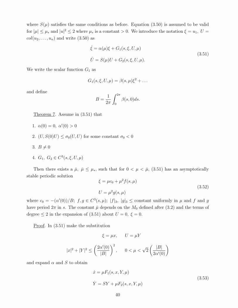
where S(µ) satisfies the same conditions as before. Equation (3.50) is assumed to be valid
for |µ| ≤ µ∗ and |u|2 ≤ 2 where µ∗ is a constant > 0. We introduce the notation ξ = u1, U =
col(u2, . . . , un) and write (3.50) as
ξ = α(µ)ξ +G1(s, ξ, U, µ)
U = S(µ)U +G2(s, ξ, U, µ).
(3.51)
We write the scalar function G1 as
G1(s, ξ, U, µ) = β(s, µ)ξ2 + . . .
and define
B =1
2π
∫ 2π
0
β(s, 0)ds.
Theorem 7. Assume in (3.51) that
1. α(0) = 0, α′(0) > 0
2. (U, S(0)U) ≤ σ0(U,U) for some constant σ0 < 0
3. B 6= 0
4. G1, G2 ∈ C3(s, ξ, U, µ)
Then there exists a µ, µ ≤ µ∗, such that for 0 < µ < µ, (3.51) has an asymptotically
stable periodic solutionξ = µc0 + µ2f(s, µ)
U = µ2g(s, µ)(3.52)
where c0 = −(α′(0))/B; f, g ∈ C3(s, µ); |f |3, |g|3 ≤ constant uniformly in µ and f and g
have period 2π in s. The constant µ depends on the M0 defined after (3.2) and the terms of
degree ≤ 2 in the expansion of (3.51) about U = 0, ξ = 0.
Proof. In (3.51) make the substitution
ξ = µx, U = µY
|x|2 + |Y |2 ≤(
2α′(0)
|B|
)2
, 0 < µ <√
2
(|B|
2α′(0)
)and expand α and S to obtain
x = µF1(s, x, Y, µ)
Y = SY + µF2(s, x, Y, µ)(3.53)
40

where S = S(0) and
F1(s, x, Y, µ) = α′(0)x+ β(s, 0)x2 + µF (s, x, Y, µ)
where |F |3 ≤ constant uniformly in µ. For µ = 0 (3.53) has a periodic solution p0 : x =
x0, Y = 0 where x0 is an arbitrary constant. It is known that for sufficiently small µ, (3.53)
will have a periodic solution pµ(s) of period 2π which for µ = 0 reduces to p0, if x0 satisfies
H(x0) =
∫ 2π
0
F1(s, x0, 0, 0)ds = 0
and H ′(x0) 6= 0. Furthermore the solution will be asymptotically stable if H ′(x0) < 0. We
see that H(x0) = 2π[α′(0)x0 + Bx20] and therefore x0 = −(α′(0))/B and H ′(x0) = −α′(0).
From the assumed smoothness of the functions in (3.53) we have pµ(s) = p0 +µp(s, µ) where
|p|3 ≤ constant uniformly in µ. Q.E.D.
6. Resonance case α(0) = i/3 (An Example)
We now discuss an example of this resonance case for the sake of completeness and to
point out the rather violent type of instability which develops as the exponents α(µ) and
α(µ) cross the imaginary axis. We consider the case in which the second equation of (3.5) is
absent. By transformations of the type (3.11) we may put the first equation of (3.5) into a
standard form similar to those obtained in Theorem 4,
w = α(µ)w + cδ(µ)eisw2 +R(w, w, s, µ).
where R is a function whose Taylor expansion about w = w = 0 contains no quadratic terms
and w = ρeiφ. We consider the case in which α(µ) = i/3 + µ, cδ(µ) ≡ 1 and R = −|w|2w,
w =
(i
3+ µ
)w + eisw2 − |w|2w. (3.60)
Letting w = zeis3 we obtain
z = µz + z2 − |z|2z. (3.61)
In polar coordinates z = reiθ this equation is
r = (µ+ r cos 3θ − r2)r
θ = −r sin 3θ.
There are seven stationary points,
r = 0
Pn : r = 1 + 0(µ), θ = n2π3
Qn : r = µ+ 0(µ2), θ = π3
+ n2π3
41

n = 0, 1, 2; and 0( ) is meant as µ → 0.* For µ > 0, the origin is an unstable node, Pn
are stable nodes and Qn are saddle points (see Fig. 9). The rays r ≥ 0, θ = n(π/3),
n = 0, 1, . . . , 5 are invariant manifolds and the disc 4 : r ≤ 5/4 is invariant as s → +∞.
Thus 4 consists of six invariant subsets
4k : 0 ≤ r ≤ 5
4, k
π
3≤ θ ≤ (k + 1)
π
3
k = 0, . . . , 5. Applying the theorem of Poincare and Bendixson to the 4k we see that the
points Pn and Qn must be joined by arcs which are solutions of (3.61). Let Γ : r = γ(θ, µ)
denote the closed curve formed by the sum of these arcs and the points Pn and Qn. Then
γ has period 2π/3 in θ. In the w, s space the original periodic solution ψ is the line w = 0
with points 2nπ identified. The z plane rotates in such a manner that when s increases by
2π, Γ sweeps out a 2-dimensional torus
τµ : w = γ(φ− s
3, µ)eiφ. (3.62)
The points Pn sweep out a stable periodic solution p = p(s, µ) of period 6π obtained by
setting φ = s/3 in (3.62). Similarly theQn sweep out an unstable periodic solution q = q(s, µ)
obtained by setting φ = s/3 + π/3. As µ > 0 tends to zero, q(s, µ) → 0 and we may say
that q bifurcates from ψ as µ increases through zero. However as µ → 0, p approaches a
limiting position p(s, 0) = eis
3 . Hence in the z plane Γ has a limiting position which consists
of three spikes 0 ≤ r ≤ 1, θ = n2π
3, n = 0, 1, 2 and we see that τµ does not bifurcate from
ψ in the sense of the definition of Chapter I, i.e., it does not collapse onto ψ as µ > 0 tends
to zero. We also see that for arbitrarily small µ > 0 there are solutions starting arbitrarily
close to ψ which run out a distance 1 + 0(µ) to the orbit p(s, µ). This is in contrast to
the non-resonance case of Section 3 where nearby solutions may run out a distance of the
order√µ to the torus (3.20). Even is the resonance case α(0) = i/4 we see, by the same
reasoning above, that the unperturbed equation (3.46) has an invariant curve Γ (Fig. 8).
Thus equation (3.43), with f1 and f2 omitted, has an invariant torus τµ lying at a distance of
the order√µ and therefore solutions starting near ψ can run out only that far. The problem
of the existence of τµ for the perturbed equation is not treated in this dissertation.
*See Titchmarsh [24] for definition of 0( ).
42

43

7. Rate of Growth of Bifurcating Manifold
We have discussed cases in which the periodic solution ψ becomes unstable and a new
stable manifold bifurcates as µ increases through zero. Since the stable oscillations of a
system are the only ones observable after a long time, it is of interest to know how these new
stable states change as the parameter µ changes. In particular, how far away is the stable
motion from the original periodic motion ψ? Such information is given by the quantity
ρ = ρ(µ) which is some appropriate measure of the distance from ψ to the stable bifurcating
manifold.* Of course for µ < 0, ψ is stable and ρ(µ) ≡ 0. Let S be the normal hyperplane
to the orbit ψ at some point of ψ. In the case in which one real root crosses the origin
(Section 5) the bifurcating manifold is a periodic solution which intersects S at some point
P . The distance from P to ψ is, in the first approximation, ρ(µ) = (constant) µ, (Fig. 10).
In the non-resonance case of Section 3 the bifurcating manifold is the torus (3.20) whose
intersection with S is, in the first approximation, a circle of radius ρ(µ) = (constant)√µ,
(Fig. 11). Also in the resonance case α(0) = i/4 the stable bifurcating manifold is the
subharmonic solution (3.40) which intersects S at a distance ρ(µ) = (constant)√µ in the
first approximation.
Thus we see that in the last two cases the bifurcation is more violent in the sense that
near the bifurcation point, ρ′(µ) becomes infinite.
For the example of the last section (α(0) = i/3), the subharmonic solution p(s, µ) inter-
sects S at a distance of 1 in the first approximation. Hence ρ(µ) is a discontinuous function
(Fig. 12)
ρ(µ) =
0 µ < 0
1 µ ≥ 0.
*See Minorsky [1] for a discussion of bifurcation and the function ρ.
44

45
CHAPTER IV
INVARIANT SURFACES
1. Introduction
In Theorem 5 of Chapter III we saw that a closed invariant surface of a vector field was
defined as the solution of a certain partial differential equation of first order involving periodic
functions. In this chapter we treat the problem of existence, uniqueness and smoothness
of the solution of a slightly more general equation. Thus we consider the real periodic
quasilinear system of first order
D(w, x, µ)w + P (x, µ)w = G(w, x, µ) (4.0)
where x = (x1, . . . , xm), w = col(w1, . . . , wn) = (uv) with u = col(u1, . . . , un1) and v =
col(v1, . . . , vn2).
P (x, µ) =
P1(x, µ) 0
0 P2(x, µ)
D(w, x, µ) = Cd =
cI1 0
0 I2
d
and
G(w, x, µ) =
(G1
G2
)= G0(x) + G(w, x, µ)
where Pj is an nj × nj matrix, Ij is the nj × nj identity, c = 1/µ > 1 and
d =m∑ν=1
aν(w, x, µ)∂
∂xν
with aν scalar functions. The functions aν , P and G are defined for
(w, x, µ) ∈ W ×R× {0 ≤ µ ≤ µ0}
with W : |w| < constant and R : 0 ≤ xi ≤ Ri a period parallelogram.
From the coefficients of d define the vector a(w, x, µ) = (a1, . . . , am) and assume that
(1) a(w, x, µ) = ω + µA(w, x, µ) if n1 > 0
(2) a(w, x, µ) = A(w, x, µ) if n1 = 0
where ω is a constant vector and
A(w, x, µ) = A0(x) + A(w, x, µ). (4.1)
46

The case n1 > 0 is the “degenerate” case mentioned in Chapter I in which the flow against
the unperturbed surface vanishes for µ = 0 (see 4.2 below).
Equation (4.0) expresses the fact that w(x, µ) = (uv) should represent an invariant surface
for the differential system
u = µP1(x, µ)u+ µG1(w, x, µ)
v = −P2(x, µ)v +G2(w, x, µ)
x = a(w, x, µ)
(4.2)
In Chapter I we considered the following differential system:
x = f(x, y, µ)
y = g(x, y, µ)(4.3)
where x and y are vectors, µ is a small parameter and the functions are periodic in x.
We assume that for µ = 0 (4.3) has an invariant surface y = φ0(x). The problem is to
find an invariant surface y = φ(x, µ) for µ ≥ 0 such that φ(x, 0) = φ0(x). If we assume
φ0(x) ≡ 0 then (4.3) can be put into the form (4.2) with the u equation absent (n1 = 0)
by setting y = µv − gy(x, 0, µ) = P2(x, µ) and a(v, x, µ) = f(x, y, µ). Then we see that
A0(x) = f(x, 0, 0).
The basic idea of the method of solution of (4.0) can be illustrated with a single equation
in one variable
a(u, x)ux + b(x)u = f(u, x) (4.4)
where x is a periodic variable and b(x) ≥ β > 0, β a constant. The equation is first replaced
by a similar equation with C∞ coefficients and right hand side. Then it is linearized by
substituting an approximate C∞ solution into the functions a(u, x) and f(u, x) to obtain the
C∞ equation
a(x)ux + b(x)u = f(x).
This equation is made elliptic by adding a higher derivative:
−εuxx + a(x)ux + b(x)u = f(x) (4.5)
with ε > 0.
The existence of a C∞ solution of this equation is then treated from the standpoint of
the classical theory (Lemma 5). We then obtain an “a-priori” estimate for the solution by
multiplying (4.5) by u to obtain.
−ε[
1
2(u2)xx − u2
x
]+
1
2a(x)(u2)x + b(x)u2 = f(x)u.
47

At the maximum of u2, (u2)xx ≤ 0 and (u2)x = 0. Hence we obtain, independently of ε,
|u|0 ≤1
β|f |0.
This estimate and similar ones for higher derivatives are then used to prove convergence of
the approximations to a solution of (4.4). The parameter ε = ε(n) goes to zero as n, the
number of iterations, goes to ∞.
2. Notation
Let A(x, µ) = (Aj1 , . . . ,jk ) be a k-dimensional array of functions defined for x ∈ R and
µ in some interval. Define
(A,B) =∑
Aj1 . . .jk Bj1 . . .jk ,
|A|0 = maxx∈R|A(x, µ)|
|A| = (A,A)12
(A,B)2 =∫R
(A,B)dx and ‖A‖ = (A,A)122 .
For r a positive integer let
∂r =∂
∂x`1
∂
∂x`2. . .
∂
∂x`r
1 ≤ `i ≤ m, denote any rth order partial derivative and let
∑[r]
=m∑`1=1i=l,...,r
.
The rth derivative of A with respect to x in an r + k dimensional array
A(r) = (∂rAj1 . . .jk) .
For r = 1 or 2 we write Ax or Axx. Then
|A(r)|2 =∑[r]
|∂rA|2 =∑[r]
(∂rA, ∂rA).
Finally define
|A|r = max0≤k≤r
|A(k)|0.
Note that the value of this norm is a function of the parameter µ. Any estimate involving
|A|r is understood to be true for each value of µ under consideration.
48

3. Main Theorem
We will now prove the existence, uniqueness and smoothness of a solution of (4.0). From
the vector A0(x) = (A01, . . . , A
0m) define the symmetric matrix
1
2
[∂A0
i
∂xj+∂A0
j
∂xi
].
Let λk(x) denote an eigenvalue of this matrix and define
λ = mink,x
λk(x).
Since A0(x) is periodic the functions ∂A0i /∂xj have zero mean value, i.e.,∫R
∂A0i
∂xjdx = 0.
In particular, the trace of the above matrix has zero mean value and thus for some k and
x, λk(x) ≤ 0. Therefore λ ≤ 0
Theorem 8. In (4.0) assume that for all x ∈ R and µ, θ ≤ µ ≤ µ0,
1. (w,P (x, µ)w) ≥ β(w,w) for some constant β > 0
2. β + rλ > 0 for some integer r ≥ 2
3. (w,P1w)− 12divA0(x) ≥ β0 > 0 for some constant β0 and all |w| = 1. If n1 = 0, replace
P1 by P2.
4. P (x, µ), G(w, x, µ), A(w, x, µ) ∈ C`(w, x)∩C(µ) for ` an integer ≥ r and |w| ≤ K, K
sufficiently large
5. max{|A|r, |G|r} = c(r,K, µ)
where c→ 0 as µ→ 0.
Define M = max{|A0|r, |G0|r, supµ |P |r}. Then there exist constants K and µ, µ ≤ µ0
such that for 0 < µ < µ, (4.0) has a unique solution w(x, µ) ∈ Cr−1(x) ∩ Lipr−1 (x) ∩ C(µ)
and |w|r−1 ≤ K. K depends only on M, β + rλ and r. µ depends on r, M, c, β, β0 and K
and in general µ decreases as r increases.
Remark. If A0(x) ≡ constant as in Theorem 5 of Chapter III, then λ = 0 and the
smoothness of the solution of (4.0) is limited only by the smoothness of the equation and the
smallness of µ. Thus if ` =∞ in (4) above then there exist intervals 0 < µ < µr, µr+1 ≤ µr
with r arbitrarily large, on which the assertion holds, i.e., w is smoother for smaller values
49

of µ. Reversing this we see that as µ increases,the number of derivatives which the theorem
guarantees is diminished.
Proof. Define β′ = β + rλ and let K be a constant
K ≥(
2
β′
)r+1
3Mr∏
(3M, 2M) + 1
where rQ is the polynomial with positive coefficients defined in Lemma 4 (proved later). We
construct successive approximations wn(x, µ) with w0 ≡ 0. This is done inductively.
Suppose wn−1(x, µ) satisfies
wn−1 ∈ C∞(x) for each fixed µ, 0 < µ < µ′ (4.30)
wn−1 ∈ Cr−1(x) ∩ C(µ) (4.31)
|wn−1|r < K.
On the set {|w| ≤ K} × R × {0 ≤ µ ≤ µ0} approximate the functions A = A(w, x, µ),
G = G(w, x, µ) and P = P (x, µ) by functions, A, G, P ∈ C∞(w, x, µ) and consider the linear
partial differential equation
Dn(x, µ)w + P (x, µ)w = Gn(x, µ)
where
Gn(x, µ) = G(wn−1(x, µ), x, µ)
and (4.33)
Dn(x, µ) = D(wn−1(x, µ), x, µ),
i.e., in the expression for D, the function A is replaced by
An(x, µ) = A(wn−1(x, µ), x, µ).
We assume the approximation to be so close that
|An − An|r + |Gn −Gn|r + |P − P |r ≤Mn (4.34)
where
Mn =1
n2min
(β′
12r,
β0
4√m,
β
4√m, M
)and the subscript r denotes differentiation with respect to x. An and Gn are defined by
(4.33) with the tildes omitted. We modify this equation still further to obtain an elliptic
equation for which the existence and smoothness of a solution is well known. Thus consider
Lnw ≡ −εn4w + Dn(x, µ)w + P (x, µ)w = Gn(x, µ) (4.35)
50

where 4 is the Laplacian in m variables, εn → 0 as n→∞ and εn > εn+1 > 0.
Define an = ω + µAn and use (4.34) to obtain(w,
[P − 1
2div anC
]w
)≥ 1
2min[β0, β](w,w)
for µ sufficiently small. Hence by Lemma 5, (4.35) has a solution w = wn(x, µ) ∈ C∞(x) for
each fixed µ. If we define p = β− β′/12 then using (4.34) we obtain (w, Pw) ≥ p(w,w). Let
λ = λ(µ) be obtained from An(x, µ) just as λ was obtained from A0(x). Then using (4.34)
and the fact that r|λ− λ| ≤ r|A0− An|` ≤ rMn + 2Krc(l,K, µ) we have p+ rλ ≥ β′/2 for µ
sufficiently small. We see here that for larger r we need smaller µ. Thus applying Lemma 4,
|wn|r ≤(
2
β′
)r+1
|Gn|rr∏(|Anxx |r−2, |P |r
).
We have|Gn|r ≤Mn + |G0|r + |G|r ≤ 2M + c′ ≤ 3M
|Anxx |r−2 ≤Mn + |A0|r + |A|r ≤ 2M + c′ ≤ 3M
and
|P |r ≤Mn + |P |r ≤ 2M
for µ sufficiently small. Differentiation is with respect to x only. G and A are as defined
in (4.1) with wn−1(x, µ) substituted for w. c′ depends on r,K and c defined in hypothesis
5 and is obtained by applying the chain rule to G and A; c′ → 0 as µ → 0. Hence from
the way K was defined, |Wn|r < K. We now verify that wn satisfies (4.31). For a function
fn(x, µ) define δfn = fn2 − fn1 = fn(x, µ2)− fn(x, µ1). From (4.35)
Ln2δwn = δGn − (δDn)wn1 − (δP )wn1
where Ln2 is Ln with µ = µ2. From the estimate of Lemma 4,
p
2|δwn|0 ≤ |δGn|0 + |δAn|0 |wn|1 + |δP |0 |wn|0.
Since |wn|1 < K this can be made small for µ2 − µ1 small. From Lemma 3, Chapter II,
|δw(j)n |0 ≤ 2Kc(j, r)|δwn|
1− jr
0
for 0 ≤ j ≤ r − 1. Thus w(j)n is continuous in µ uniformly in x. Since wn ∈ C∞(x) for fixed
µ, we have wn ∈ Cr−1(x)∩C(µ). Thus for µ′ sufficiently small and fixed we have a sequence
{wn} satisfying (4.30)-(4.32).
To show convergence define δn+1 = wn+1 − wn. Then from (4.35) Ln+1δn+1 = H where
H = Gn+1 − Gn −4wn(εn − εn+1)− (Dn+1 − Dn)wn.
51

From the estimate of Lemma 4
|δn+1|0 ≤2
p|H|0.
We have|(Dn+1 − Dn)wn|0 ≤ [2Mn + |An+1 − An|0]K
≤ 2KMn +K|Aw|0 |δn|0where An = A(wn−1, x, µ). Similarly
|Gn+1 − Gn|0 ≤ 2Mn + |Gw|0 |δn|0
and
|4wn|0 ≤√m |wn|2.
But |Aw|0 = |Aw|0 ≤ c(1, K, µ) and |Gw|0 = |Gw|0 ≤ c(1, K, µ). Thus for µ sufficiently small
|δn+1|0 ≤1
2|δn|0 + qn
where
qn = 8Kp−1Mn + 2p−1√m(εn − εn+1).
Since Σ∞1 qn <∞ we see that Σ∞0 |δn+1|0 <∞ and hence the wn converge uniformly in x and
µ.
Letting z = wn+p − wn, p > 0 an integer, we have, using Lemma 3,
|z(j)|0 ≤ 2Kc(j, r)|z|1−jr
0
for 0 ≤ j ≤ r−1. Thus the sequence {wn} converges to a limit function w ∈ Cr−1(x)∩C(µ).
The Lipschitz condition follows from
|w(r−1)n (x1, µ)− w(r−1)
n (x2, µ)| ≤ |wn|r|x1 − x2|
≤ K|x1 − x2|
and passing to the limit. For uniqueness assume w1 and w2 ∈ C1(x) ∩ C(µ) are solutions of
(4.4) and satisfy |wi|1 ≤ K. Then δw = w2 − w1 satisfies the linear equation
D2δw + Pδw = δG− (δD)w1
where
D2 = D(w2, x, µ), δG = G(w2, x, µ)−G(w1, x, µ)
and
δD = D(w2, x, µ)−D(w1, x, µ).
52

Now apply Lemma 4 in the ε = r = 0 case to obtain
β
2|δw|0 ≤ |δG|0 + |δA|0K
= |δG|0 + |δA|0K
≤ (|Gw|0 + |Aw|0K)|δw|0
≤ β
4|δw|0
for µ sufficiently small (Hypothesis 5). Thus |δw|0 = 0. Q.E.D.
4. “A-priori” Estimates and Solution of Linear Problem
We now derive some estimates appropriate for a solution of the real linear elliptic partial
differential equation
Lw ≡ −ε4w +D(x, µ)w + P (x, µ)w = G(x, µ) (4.40)
where x = (x1, . . . , xm), w andG are column n-vectors with w = (uv) u = col(u1, . . . , un1), v =
col(v1, . . . , vn2),
D = Cd =
cI1 0
0 I2
d,c =
1
µ> 1
Ij = nj × nj identity
with
d =m∑ν=1
aν(x, µ)∂
∂xν, aν scalar and
P (x, µ) =
P1(x, µ) 0
0 P2(x, µ)
, Pj an nj × nj matrix.
From the coefficients in d we have the vector a(x, µ) = (a1, . . . , am) where (1) a(x, µ) =
ω + µA(x, µ) if n1 > 0 or (2) a(x, µ) = A(x, µ) if n1 = 0 where ω is a constant vector. We
assume A = A(x, µ), P = P (x, µ) and G = G(x, µ) are defined for (x, µ) ∈ R× Iµ where R
is a period parallelogram and Iµ : 0 < µ < µ.
Consider the symmetric matrix
1
2
[∂Ai∂xj
+∂Aj∂xi
]and let λk(x, µ), k = l, . . . ,m denote the eigenvalues. Define
λ′ = infµ
mink,x
λk(x, µ)
53

and note that λ′ ≤ 0 due to the periodicity of A and the same argument as given before
Theorem 8.
Lemma 4. “A-priori” Estimates
Assume ε ≥ 0 and for r ≥ 0 an integer, assume
1. A,P,G ∈ Cr(x) for each fixed µ ∈ Iµ and w ∈ C`(x); ` = r + 2 if ε > 0, ` = r + 1 if
ε = 0.
2. (w,Pw) ≥ β(w,w) for (x, µ) ∈ R× Iµ where β > 0 is a constant
3. β + rλ′ > 0.
Then
|w|0 ≤2|G|0β
and in general for 0 ≤ s ≤ r
|w|s ≤|G|s
s∏(|Axx|s−2, |P |s)
(β + sλ′)s+1(4.41)
for all µ ∈ Iµ, where for k < 0, | |k is taken to be zero. sQ(a, b) is a polynomial in a and b of
degree s having positive coefficients which depend only on s. The estimates are independent
of ε.
Proof. Due to the form of P and the fact that 4 and D are diagonal operators, (4.40)
has the form
−ε4u+ cdu+ P1u = G1 (4.42)
−ε4v + dv + P2v = G2. (4.43)
We have |w|0 ≤ |u|0 + |v|0 ≤ 2|w|0, |P |0 ≤ |P1|0 + |P2|0 ≤ 2|P |0 and (v, Pjv) ≥ β(v, v) for
j = 1 and 2. We obtain the estimate for (4.43) and note that the estimate for (4.42) follows
by replacing a by ca.
Multiply (4.43) by v (scalar product) and use the identities
(v,4v) =1
24(v, v)− |vx|2
(v, dv) =1
2d(v, v)
to obtain
−ε[
1
24(v, v)− |vx|2
]+
1
2d(v, v) + (v, P2v) = (v,G2).
54

Let x0 be a point at which (v, v) is a maximum, i.e., at x0, (v, v) = |v|20. Since 4(v, v) ≤ 0
and d(v, v) = 0 at x0 we obtain (v, P2v)|x=x0 ≤ (v,G2)|x=x0 and therefore β|v|0 ≤ |G2|0.
To obtain the general estimate (4.41) we assume the solution has a sufficient number
of derivatives and apply the same argument to the differentiated equation. The rule for
applying ∂s to a product fg of two functions is
∂s(fg) = f(∂sg) +s∑j=1
∂f
∂x`j
(∂s−1j g
)+ . . .
where
∂s−1j =
∂
∂x`1· · · ∂
∂x`j−1
∂
∂x`j+1
· · · ∂
∂x`s
and the dots (present only if s ≥ 2) represent a sum which is bilinear in f and g involving
derivatives of f of order ≥ 2. Thus
∂s(dv) = d(∂sv) +Qs +Rs
where
Qs =s∑j=1
m∑ν=1
∂aν∂x`j
∂
∂xν
(∂s−1j v
)and
Rs =∑ν
p+q=s+1l≤p≤s−1
[v(p) ∗ a(q)ν ]
where Rs ≡ 0 for s ≤ 1, Qs ≡ 0 for s = 0 and the ∗ notation denotes a linear combination
of terms ∂pv∂qaν . Now apply ∂s to (4.43), multiply by ∂sv and sum to obtain∑[s]
{−ε[
1
24(∂sv, ∂sv)− |∂svx|2
]+
1
2d(∂sv, ∂sv)
+(∂sv, P2∂sv +Qs)} = H
(4.44)
where
H =∑[s]
(∂sv, ∂sG2 + Rs)
with
Rs = −Rs +∑t+p=s
0≤p≤s−1
[P
(t)2 ∗ v(p)
].
We now show that ∑[s]
(∂sv, P2∂sv +Qs) ≥ (β + sλ′) |v(s)|2. (4.45)
55

From the assumption (2), ∑[2]
(∂sv, P2∂sv) ≥ β
∑[s]
(∂sv, ∂sv)
= β |v(s)|2.
For the second part, S, we have
S ≡∑[s]
(∂sv,Qs) =
n2∑i=1
∑[s]
∂svi(Qs)i
=
n2∑i=1
s∑j=1
m∑`p=1
p=1,...,sp 6=j
m∑
ν,`j=1
∂aν∂x`j
[∂
∂xν
(∂s−1j vi
)]∂svi
.
The term in braces is a quadratic form,
K ≡m∑
ν,`j=1
αν,`jξνeξ`je,
where
αν,`j =∂aν∂x`j
, ξνe =∂
∂xν
(∂s−1j vi
)ξ`je = ∂svi = ∂
∂x`j
(∂s−1j vi
)and e is the vector of subscripts
e = (i, `1, . . . `j−1, `j+1, . . . `s).
From the way in which λ′ is defined,
K ≥ λ′m∑k=1
ξ2ke
and therefore
S ≥ λ′s∑j=1
n2∑i=1
m∑k,`p=1p=1,...,sp 6=j
[∂
∂xk
(∂s−1j vi
)]2
= λ′s∑j=1
|v(s)|2 = sλ′|v(s)|2
which proves (4.45). We now repeat the argument after (4.43) where x0 is a point at which
|v(s)|2 ≡∑[s]
(∂sv, ∂sv)
56

is a maximum to obtain
(β + sλ′)|v(s)|0 ≤ |H|0 ≤ |G(s)|0 + |Rs|0.
Using the fact that
[β + sλ′] ≤ [β + (s− 1)λ′] ≤ . . . ≤ β + λ′ ≤ β ≤ |P |0 (4.46)
we write this as
(β + sλ′)s+1|v(s)|0 ≤ βs|G|s + [β + (s− 1)λ′]s|Rs|0.
We now prove (4.41) inductively. Assume it is true with s replaced by 0, 1, . . . , s − 1. The
expression Rs is linear in v and each term contains a factor ∂ρv with ρ ≤ s − 1. Using the
induction assumption and (4.46) we obtain
(β + sλ′)s+1|v(s)|0 ≤ |G|ss∏′
(|Axx|s−2, |P |s)
wheres∏′
is a polynomial of the type described after (4.41). (Note: |ax| = |µAx| ≤ |Ax|since 0 < µ < 1. In deriving the estimate for u in (4.42) we get |cax| = |Ax| and hence the
estimates are exactly the same.) From (4.41), with s replaced by s− 1, we have
(β + sλ′)s+1|v|s−1 ≤ |G|ss∏′′
(|Axx|s−2, |P |s)
where we have again used (4.46) and the fact that | |p ≤ | |q for p < q.
Now defines∏
to be the polynomial whose coefficients are twice the maximum of the
corresponding coefficients ins∏′
ands∏′′
. Then (4.41) follows since
|v|s = max(|v(s)|0, |v|s−1).
In regard to the assumption made on ` in (1), note that in (4.44) for s = r we need
v ∈ Cr+2 if ε > 0 and v ∈ Cr+1 if ε = 0. Q.E.D.
Finally comes the problem of existence of a solution of equation (4.40), Lw = G. We
no longer employ the maximum norm used in the solution of the quasi-linear equation, but
introduce the Hilbert space of square integrable functions having period parallelogram R.
By obtaining an “a-priori” estimate for a solution of the adjoint equation we prove the
existence of a “weak” solution of Lw = G. The proof follows that of Friedrichs [12; p. 353].
Certain difficulties, which arise in considering domains with boundaries, disappear due to
the periodicity. The C∞ differentiability of the weak solution then follows from a result of
P. D. Lax [23]. The following lemma is a statement of these classical results.
57

Lemma 5. - (Existence) In (4.40) assume
1. ε > 0
2. (w, [P (x, µ)− 1
2div a(x, µ)C]w) ≥ p(w,w) for (x, µ) ∈ R× Iµ and p > 0 a constant
3. for each µ ∈ Iµ, A, P,G ∈ C∞(x).
Then for each fixed µ ∈ Iu, (4.40) has a unique solution w(x, µ) ∈ C∞(x).
Proof. For the equation Lw = G we have∫R
(w,Lw) =
∫R
(w,G)
and integrating by parts
ε
∫R
|wx|2 +
∫R
(w, [P − 1
2div a C]w) =
∫(w,G)
where periodicity was used to drop out the boundary terms. From this we obtain
‖w‖ ≤ 1
p‖G‖. (4.47)
For the adjoint operator L∗φ ≡ −ε4φ − D(x, µ)φ + P (x, µ)φ with P = P − (div a)C, we
obtain the same estimate
‖φ‖ ≤ 1
p‖L∗φ‖ (4.48)
Let L2(R) denote the Hilbert space of functions f(x), x ∈ R, such that ‖f‖ < ∞. Using
(4.48), for each fixed µ, we prove the existence of a “weak” solution of Lw = G, i.e., a
function w(x, µ) ∈ L2(R) such that (w,L∗φ)2 = (G, φ)2 for all φ in a dense subset of L2(R).
For defineQ = {q : q = L∗φ, φ ∈ C∞(x), x ∈ R, φ
periodic with period parallelogram R}
On Q define the functional ψ(q) = (G, φ)2. The estimate (4.48) implies uniqueness for
the adjoint equation and hence ψ is well defined, i.e., given q ∈ Q, there is exactly one
φ ∈ C∞(x) such that q = L∗φ. ψ is bounded and linear due to (4.48) and the linearity of
L∗. Thus by Riesz’s representation theorem ψ(q) = (w, q)2 for some w(x, µ) ∈ L2(R), i.e.,
(G, φ)2 = (w,L∗φ)2.
In the previous reference to P. D. Lax, it is shown that for such a weak solution w(x, µ),
if G and the coefficients of L have derivatives in x up to order t which are in L2(R) then
58

w(x, µ) has derivatives in x up to order t+ 2 which are in L2(R). This implies, by Sobolev’s
lemma, that w(x, µ) ∈ Cr(x) where r = t − [m/2] + 1. Hence in our case w(x, µ) ∈ C∞(x)
for each fixed µ.
Uniqueness follows from the estimate (4.47).
Q.E.D.
5. An Example of Non-parallelizable Flow
The following is an example of the situation described in Chapter I in which the flow on
the unperturbed surface τ(0) is not parallelizable. Here τ(0) is a 2-dimensional torus having
1-dimensional invariant submanifolds which intersect at stationary points (Fig. 13).
θ1 = −k1 sin θ1 + µF1(y, θ1, θ2, µ)
θ2 = −k2 sin θ2 + µF2(y, θ1, θ2, µ)
y = −y + µG(y, θ1, θ2, µ)
where ki > 0 are constants, y is distance measured along the normal to the surface and Fi
and G ∈ C∞ in all arguments.
In this example β = 1 and λ = −max(k1, k2). Applying Theorem 8 we see that if
−λ < 1/r, r an integer ≥ 2, then for µ sufficiently small there exists an invariant manifold
y = ψ(θ1, θ2, µ) where ψ has r− 1 Lipschitz continuous derivatives with respect to θ1 and θ2
and is continuous in µ with ψ(θ1, θ2, 0) ≡ 0.
59

60

BIBLIOGRAPHY
1. Minorsky, Nicholas, Nonlinear Oscillations. New York: D. Van Nostran Company,
Inc., 1962, Chapter 7.
2. Hopf, E., “Abzweigung einer periodischen Losung von einer stationaren Losung eines
Differentialsystems,” Sachs. Akad. Wiss. Leipzig, Math-Phys. Klasse, Berichten. XCIV
Band, Sitzung 19. Jan. 1942.
3. Hopf, E., “Repeated Branching through Loss of Stability - an Example,” Proc. Conf. Diff. Eqns.
Univ. Maryland, Mar. 1955 (Bound volume: Univ. Maryland book store 1956).
4. Coddington, E. A. and Levinson, N., Theory of Ordinary Differential Equations. New
York: McGraw-Hill Book Company, Inc., 1955, p.362.
5. Diliberto, Stephen P., “Perturbation Theorems for Periodic Surfaces - I,” Rendiconti del Circolo Matematico di Palermo.
Series II, Tomo IX, pp. 265-299.
6. Diliberto, Stephen P., “Perturbation Theorems for Periodic Surfaces - II,” Rendiconti del Circolo Matematico di Palermo.
Series II, Tomo X, pp. 111-161.
7. Bogoliubov, N. N. and Mitropolsky, Y. A., Asymptotic Methods in the Theory of Nonlinear Oscillations.
New York: Gordon and Breach publishers, 1961, Chapters 5 and 6. (English transla-
tion from Russian).
8. Bogoliubov, N. N. and Mitropolsky, Y. A., “The Method of Integral Manifolds in
Nonlinear Mechanics,” Contributions to Differential Equations. Vol. II, Nos. 1-4,
1963, pp. 123-196.
9. Hale, Jack K., “Integral Manifolds of Perturbed Differential Systems,” Annals of Mathematics.
Vol. 73, No. 3, 1961, pp.496-531.
10. Hale, Jack K., “On the Method of Krylov-Bogoliubov-Mitropolsky for the Existence of
Integral Manifolds of Perturbed Differential Systems,” Boletin de la Sociedad Matematica Mexicana.
1960.
11. Diliberto, S. P. and Hufford, G., “Perturbation Theorems for Nonlinear Ordinary
Differential Equations,” Contributions to the Theory of Nonlinear Oscillations (S. Lef-
schetz). Vol III, 1956, pp. 207-236.
12. Friedrichs, K. O., “Symmetric Positive Linear Differential Equations,” Communications on Pure and Applied Math.
Vol XI, No. 3, August 1958, pp. 333-418
61

13. McCarthy, John, “The Stability of Invariant Manifolds - Part I,” Technical Report
No. 36, Office of Naval Research, Applied Math. and Statistics Lab., Stanford Univ.,
Stanford, Calif., Feb. 1955.
14. Kyner, Walter T., “Invariant Manifolds,” Rendiconti del Circolo Matematico. Series
II, Tomo IX, 1961, pp. 98-110.
15. Levinson, Norman, “Small Periodic Perturbations of an Autonomous System with a
Stable Orbit,” Annals of Mathematics. Vol. 52, No. 3, Nov. 1950, pp. 727-738.
16. Lefschetz, Solomon, Differential Equations: Geometric Theory - Second Edition. New
York: Interscience Publishers, 1963.
17. Segre, Beniamino, Some Properties of Differentiable Varieties and Transformations. Berlin-
Gottingen-Heidelberg: Springer-Verlag, 1957, Part 2.
18. Kelly, A., “Using Change of Variables to Find Invariant Manifolds of Systems of Ordi-
nary Differential Equations in a Neighborhood of a Critical Point, Periodic Orbit, or
Periodic Surface - History of the Problem,” Technical Report No. 3, Office of Naval
Research, Dept. of Math., Univ. of Calif., Berkeley, May 1963.
19. Moser, Jurgen K., “On Invariant Curves of Area-Preserving Mappings of an Annulus,”
Akad. Wiss. Gottingen, Math.-Phys. Klasse Nachrichten. No. 1, 1962, pp. 1-20, (In
particular pp.10-12).
20. Nemytskii, V. V. and Stepanov, V. V., Qualitative Theory of Differential Equations.
Princeton, N.J.: Princeton Univ. Press 1960, pp. 249-252 (English translation from
Russian).
21. Malkin, I. G., Some Problems in the Theory of Nonlinear Oscillations. (Book 1). Moscow,
1956, (U.S. Atomic Energy Comm. translation AEC-tr-3766 (Book 1), p. 207).
22. Birkhoff, G. D., Dynamical Systems. Providence, R. I.: Amer. Math. Soc. Colloq.
Publications, Vol. IX, 1927, p. 69.
23. Lax, Peter D., “On Cauchy’s Problem for Hyperbolic Equations and the Differentiabil-
ity of Solutions of Elliptic Equations,” Communications on Pure Applied Math., Vol.
VIII, No. 4, Nov. 1955, pp. 615-633.
24. Titchmarsh, E. C., The Theory of Functions - Second Edition. London: Oxford Uni-
versity Press, 1939, p. 1.
62