1

New York City Crime Declines - Methodological Issues*

David F. GreenbergSociology DepartmentNew York University

295 Lafayette St. 4 FloorNew York, NY 10012(212) 998-8345 (tel).

dg4@nyu.edu

For presentation to the John Jay Conference on the New York City Crime Drop

September 2011

*This text is not a paper in the usual sense. It was written to be the methodology section of a grantproposal.

2

New York City Crime Decline - Methodological Issues

Research dealing with the exceptionally steep crime decline seen in New York City in the

decade of the 1990s, and its continuation in the first decade of the 21 century when crime ratesst

leveled off in many other cities, must deal with a number of methodological issues. Much of the

abundant research literature already published on this subject (Chauhan, Preeti, n.d.) evinces

weaknesses on methodological points, and as a result, it does not provide definitive explanations of

the New York crime decline. This includes both studies of variation between neighborhoods within

the city of New York, and studies that compare New York with other cities. I discuss several of these

methodological concerns, with particular attention to the identification of optimal strategies for

improving on the earlier work.

VARIABLE SELECTION

Any statistical study designed to assess the influences of possible causes on their putative

effects must begin by choosing the variables that will represent the effects or outcomes, and those

that will represent their supposed causes. In popular discourse one hears of the “crime rate” but there

are actually numerous crime rates or counts. For this study it would make sense to focus primarily

on the 8 offenses classified by the FBI as “index offenses” (which are murder and non-negligent

homicide, forcible rape, aggravated assault, robbery, burglary, grand larceny, motor vehicle theft,

arson). These are likely to be the best measured, i.e. trends in the reported volume of these crimes

are most likely to reflect underlying crime patterns, with the least distortion by changes in reporting,

For decades, criminologists have understood that under-reporting and under-recording1

lead to measurement error in officially- constructed crime rates. Initially this led to concern thatthere was more crime than thought. For our purposes, the accuracy of point estimates of crimerates is unimportant. It is changes in those estimates that are important. Relatively little is knownabout changes in reporting and recording practices, especially as these vary across locations.These sorts of variations could potentially distort comparisons of change in crime rates acrossjurisdictions. The difficulty of studying these effects has led criminologists to ignore them.

Pro-active policing will also be important in the generation of crime rates for some non-2

index crimes, particularly the possession and sale of illegal drugs.

Corman and Mocan (2000) raise another slight complication when they observe that the3

population figures for New York neighborhoods are controversial. For this reason theyrecommend using counts. They do not indicate what is controversial about these numbers, or whythis is a good remedy. One suspects that the issue is the extent of under-counting. This might be aparticularly important issue where there are many illegal immigrants. This could be an importantsource of measurement error in various parts of the United States, not just in New York. Onewould expect researchers to control statistically for changes in precinct populations over time inan analysis of counts. Failure to do so would risk specification bias. The matter meritsinvestigation, for if population counts suffer from measurement error problems, this will affectthe analyses. New Orleans illustrates this point. It has been alleged that following Hurricane

3

and in police enforcement and recording practices. Counts of crimes charged as misdemeanors, such1

as prostitution, disorderly conduct, and so forth are, on the face of it, very likely to be substantially

influenced by decisions by police departments to crack down on certain kinds of offenses, or to give

them a lower priority in law enforcement, unlike the major felonies. For example, arrests for

possession of marijuana have risen more than ten-fold in New York in the last quarter-century, with

no evidence that this rise was occasioned by an increase in the extent of use or sale (Drug Policy

Alliance, 2011; Speri, 2011). Decisions about where in a city to assign police, policies and practices

regarding stops, frisks and searches, and to ignore or to make an arrest in public order cases, will all

influence recorded crime rates for misdemeanors far more than for the index crimes. Reservations2

about the validity of misdemeanor counts as a measure of crime do not, it should be emphasized,

preclude the use of arrests for misdemeanors as a possible influence on crime rates. This supposed3

Katrina, the Census Bureau was under pressure not to show a large population decline, and so itover-estimated the population. In later years it supposedly provided more accurate (smaller)figures, making it look like a big increase in the crime rate had taken place.

4

influence has figured in controversies regarding “order-maintenance” policing in New York. It is a

matter of considerable public interest to resolve questions as to what effect this type of policing

strategy has on serious crime rates.

A complication is that counts of all eight index crimes are not equally reliable. Corman and

Mocan (2000) observe that in 1986, the definition of grand larceny in New York changed, making

it difficult to use in analyses going back farther than that in time. Similar definitional changes may

have been made in other cities as well. If they all occurred at the same time, this can easily be taken

into account. If the changes occurred at different times, and those times are unknown, there is a

potential for bias. Corman and Mocan (2000) also say that they found rape counts to have fluctuated

too much from year to year to be considered trustworthy. In addition, Rosenfeld (2007) notes that

definitions of assault changed over time.

Even if index crimes are, on the whole, measured more precisely than misdemeanors, the

accuracy of the New York police departments’ felony crime counts cannot be taken for granted. For

as long as New York mayors and police superintendents have been boasting of their success in

reducing crime, academically-based criminologists (Eli Silverman, Andrew Karmen) and journalists

writing for the broader public (in such venues as The Village Voice) have contended that political

and administrative pressures have led to undercounts of crimes through such procedures as not

accepting or recording complaints of victimization, or of recording them as offenses less serious than

is warranted by the facts of the case. These behaviors are allegedly responses to administrative

pressures on police captains to reduce crime rates in their precincts.

5

In principle there are ways of checking some of the New York Police Department’s numbers.

In a lecture given at the New York University School of Law in the fall of 2010, Franklin Zimring

spoke of research he has been carrying out on the great New York crime decline, to check the

accuracy of NYPD crime figures. This entailed, for example, looking at reports of automobile theft

to insurance companies, and homicide counts as listed by the Center for Disease Control. His

conclusion was that for purposes of studying the crime decline, NYPD numbers were quite accurate,

though not 100% perfect. This is reassuring. However, the following week, the Village Voice

reported that hospital emergency room episodes involving aggravated assault did not show good

correspondence with NYPD data. Hospital cases were going up, while NYPD figures were showing

that assaults were dropping. The New York Post dismissed this discrepancy, asserting that hospitals

were increasingly likely to report emergency assault cases to the police, bringing about a perceived

rise that was not real. However, it provided no source for this claim. The matter needs to be looked

into.

In recognition of the criticisms that NYPD -produced crime counts have received, Police

Commissioner Raymond W. Kelly has recently announced the appointment of an external review

panel to review the statistics (Baker and Rashbaum, 2011). Even if it should turn out that New York

City’s crime statistics are sound, a comparison of New York City with other cities will entail the use

of crime counts from those cities as well. The accuracy of those counts is likely to be unknown and

unverifiable in almost all cases.

Most criminologists use agency-generated counts while ignoring the potential bias that errors

in these counts could be producing, or they have restricted their analyses to homicides, arguing that

the necessity of explaining a dead body is likely to make homicide counts more accurate than counts

In 2010, the number of blacks killed in New York rose by 31%, while the number of4

whites killed fell by 27% (Wills, Bennett-Smith and Parascandola, 2011). These divergenceswould be obscured in an analysis of overall killings not broken down by race.

6

for other serious crimes. However, even this cannot be taken for granted.

Where possible, it would be desirable to compare tallies of homicides assembled by the FBI in its

annual Uniform Crime Reports and Supplemental Homicide Reports on the basis of reports from

police departments with those from other sources, such as the National Center for Health Statistics,

and the vital statistics tables produced by individual state agencies. These should be consulted and

compared to assess the validity and reliability of the homicide counts to be used in this study. It is

my understanding that divergences in these tallies have developed in recent years due to incomplete

agency reporting and delays in reporting. It may be that a way can be found to draw on multiple

sources to construct an improved homicide count. Regrettably, victimization data of the sort

produced by the National Criminal Victimization Survey are not available at the city level.

In the case of homicide, it would also be desirable to analyze disaggregated rates, that is,

homicide rates for specific classes of victims, defined by age, race and sex. This is because the

causes of changes in homicide rates may be better illuminated if the patterns for specific classes of

individuals are distinct. For example, if we learn that homicide deaths among young black males in

the mid-1980s were elevated, but that victimization rates for older blacks, and for members of other

races, did not experience a comparable upsurge, this might point us to causal mechanisms that

distinguish the ages and races of homicide offenders. (Blumstein and Rosenfeld, 1998; Pritchard4

and Buler, 2003).

UNIT OF ANALYSIS

What should the unit of analysis be? For an analysis of changes in crime rates undertaken

7

for the purpose of identifying local conditions that led some parts of the city to experience greater

or lesser drops than others, data providing information on local crime rates and area conditions are

needed. No pre-existing data set is going to be perfect for this purpose. Practical considerations will

force the use of data sets compiled by city government agencies. The NYCPrecinct data set is likely

to be as good a data st as one would be able to get.

For purposes of understanding what made New York distinct from other cities, the choice

of unit of analysis is less obvious. Here are the main options: (1) One could take the city as a unit.

This is a potentially problematic choice, because the crime decline may not have occurred uniformly

throughout the city. If it occurred only in certain neighborhoods or boroughs, an analysis that was

based on treating the city as a unitary entity could fail to see processes that were important, because

the city-wide characteristics used in the analysis might not adequately characterize the particular city

areas where decline took place. In that connection, Steven Levitt (2001) observed in a commentary

on a national analysis of crime that neighborhood-level unemployment rates in Chicago in one year

ranged from 3% to 41%. To use a city-wide average to characterize the city would be to wash out

its within-city neighborhood variability. It is well known that crime rates vary greatly from one

neighborhood to another, and a good deal of criminological research have been invested in

understanding whether temporal trends in crime rates vary across neighborhoods (Kubrin and

Herting, 2003; Weisburd et al, 2004).. An important question to address early in the analysis, then,

is: was the crime decline fairly uniform from one neighborhood to another? Or were there sharply

divergent patterns in different neighborhoods?

Preliminary Precinct-Level Analyses

To answer to this question, I carried out some preliminary analyses by using the

A fuller analysis would want to update the present data set, which ends in the year 2001.5

Crime counts for New York precincts are now available from the NYPD web site going up to2009. This addition would be important for statistical reasons (more observations means morestatistical power) and for substantive reasons. I believe that in the decade of the 1990s, NewYork’s crime decline was only moderately greater than that in many other cities (privatecommunication from Al Blumstein). More striking, that decline continued in the next decade,when crime rates in other cities had leveled off. Judging from the counts for 2010 listed on theweb site of the New York Police Department, the decline in violent felonies may have reversed.Homicides, for example increased from 471 in 2009 to 536 in 2010. This is an increase of 13.8%.Year-to-date figures for 2011 show a continued increase, from 310 to 349.

8

NYCprecinct data set furnished to me by Richard Rosenfield. This data set contains information

about crime and several dozen explanatory variables for New York precincts for the years 1988-

2001. All of these variables were treated as independent causes, rather than as imperfect measures5

of a latent variable. The latter approach might lead researchers to use factor analysis to construct

indexes representing neighborhood “concentrated disadvantage” or other concepts. This approach

has been used fruitfully in some studies of urban crime patterns (e.g. Rosenfeld, Fornango and

Rengifo, 2007; Messner et al., 2007), and is likely to be promising in future research. It should

improve the accuracy with which the impact of socio-economic status is measured.

After considering the results of the preliminary analyses, I will argue that a precinct-level

analysis is likely to be too limited in scope to provide definitive answers to the New York anomaly.

It does, however, offer the potential for understanding neighborhood variation in crime trends. Most

of the methodological issues treated here in the context of a study of precincts would also arise in

studying larger political units such as cities or counties. Consequently this discussion has

considerable relevance to the explanation of inter-city variation. I discuss these methodological

issues in this section so that the points can be illustrated with actual data.

The first step in my analysis was to regress the logged crime rates on time separately for

This is accomplished with the Stata syntax statsby _b, by(precinctid) verbose nodots:6

regress lncrimerate time.

9

each of the 75 New York precincts, save the regression coefficients, and then look at the estimates

and their distributions. Table 1 lists the precinct-specific intercepts and regression coefficients for6

the logged homicide rate, while Figure 1 shows the distribution of estimates graphically. The table

and histogram show that all the slopes are negative. The intercepts, which are also listed, are of less

interest here. They simply show that the homicide rates found in some precincts are higher than

those in others, which is well known. Our interest lies in the slopes, which measure change in these

rates over time. Homicides dropped in every precinct, although more in some than in others. The

correlation between the individual intercepts and the individual slopes is -.85, indicating that

homicides dropped much faster in high-homicide precincts than in low-homicide precincts.

_____________________________________________________________________________

Insert Table 1 and Figure 1 about here.

_____________________________________________________________________________

Table 2 shows the intercepts and slopes for the logged robbery rates, and Figure 2 shows the

corresponding histogram. Every precinct but one sustained a drop in the robbery rate, albeit a larger

drop in some precincts than in others. Robbery rates rose in that one precinct by a very small amount

(Precinct 20 on the Upper West Side was the exception). For this offense, the correlation between

the individual intercepts and slopes was -.73.

______________________________________________________________________________

Insert Table 2 and Figure 2 about here.

______________________________________________________________________________

Weisburd et al. (2004) come to the opposite conclusion in their study of crime7

trajectories for Seattle neighborhoods. However, their results show that the 18 distincttrajectories they claim to have identified for Seattle neighborhood crime rates differ from oneanother mainly in their levels. There are some differences in slopes as well, but they are ofmodest magnitude. Truly distinct slopes were present only in a tiny number of neighborhoods.

I am not sure what the word “complaints” means in this data set. Are these complaints8

initiated by citizens, or by police, or both?

10

For assaults, the rates fell in every precinct except 20 and 23, where they rose by a very small

amount (see Table 3). For this offense, the correlation between intercepts and slopes was -.58.

Though the precincts in which crime rates did not fall may warrant special investigation to discover

how they differed from the rest of the city, the exceptions to the generalization that crime fell are so

few that it seems reasonable to treat the city as a whole as a unit for purposes of comparison with

other cities. However, because the rates of decline did vary among precincts for all three offenses,7

an analysis this within-city variation in trends would also be worthwhile.

______________________________________________________________________________

Insert Table 3 and Figure 3 about here.

______________________________________________________________________________

When I repeated this type of analysis using misdemeanors and violations as dependent

variables, I found that in most precincts, misdemeanor complaints rose (See Table 4). Only in 118

precincts did they fall. Most of those precincts had low precinct numbers. This pattern could be

explained in various ways. Conceivably, the factors that led to the fall of violent felonies led to the

rise of misdemeanors. Alternately, misdemeanor complaints are much more influenced by police

initiatives than are violent felony complaints. One may speculate that as felony arrests fell, the police

went out looking for minor infractions to keep themselves busy, or to justify their budgets and

British property crime rates, for example, began dropping in the mid-1990s.9

11

staffing levels, or that they had more resources for policing lesser offenses. Alternately, they may

have been operating on the belief that making arrests for misdemeanors reduces felony crime. It

could also be that the threat of serious penalties for felonies pushed prospective criminals to take

up less serious misdemeanors. Instead of desisting from crime altogether, they may have shifted from

felonies to less serious crimes. The trends in logged violation rates, shown in Table 5, against show

that most precincts had a rise in violations; only in five of the seventy-five did they fall (See Table

5).

_____________________________________________________________________________

Insert Tables 4 and 5 about here.

______________________________________________________________________________

One may think that a fall in felonies in all or almost all precincts between 1988 and 2001

could have been due to changing levels of precinct characteristics; or it could have been due to some

other factors not measured by the variables in the data set. Given that the crime drop occurred in

many American cities - and in cities in other parts of the world - it is not likely that the factors 9

responsible for the big drop in New York were totally distinct to New York. This reasoning points

to national trends that may have occurred more strongly in some cities than in others. Still, these

global changes would not explain the variability in the magnitude of changes between precincts. It

is to that subject we now turn.

To assess the plausibility that changes in levels of the predictors were responsible for trends

in the crime rates, I pooled the data set, and used the xtreg command in version 11 of Stata to assess

the average impact of the various regressors on the logged crime rates. This estimation was done

A panel data set consists of observations for multiple objects (e.g., people or cities) at10

multiple times. Usually those time points are evenly spaced, though for some types of analysisthis is not required. In the analyses discussed here, the time points are one year apart.

12

separately for homicide, robbery and assault. In these preliminary analyses I treated all neighborhood

conditions represented in the data set as potential candidates for causes, and interpret the estimates

using causal language. It should be kept in mind, however, that for reasons mentioned later, an

independent variable could make a significant contribution to an estimation without being a direct

cause of the dependent variable

In carrying out this analysis, some attention must be given to the manner in which non-

independence of observations is handled in this analysis. In a panel data set, observations for N10

precincts at T times, yielding NT observations, are not equivalent to NT observations for as many

precincts, measured at a single point in time. When multiple observations are collected for each

object in the data set, those observations are not statistically independent. Observations of a variable

measured in the same precinct at different times are more likely to be close together than

observations of cases from different precincts. If this is the case, conventional inferential statistics

are not valid, and in typical panel data analyses, the bias can be large. To a degree, this type of

heterogeneity can be taken into account by introducing variables measuring known sources of

heterogeneity into the analysis (e.g. demographic and economic characteristics).

Commonly, this strategy does not deal adequately with heterogeneity. It may account for

some of the heterogeneity, but often it does not do so completely. This is because there are likely

to be unmeasured sources of heterogeneity. They may be unmeasured because the researcher didn’t

think of them, or because data for them were not to be had. If we denote an unmeasured stable

Note that no subscript for time is present here. That is because we are assuming the11

characteristic to be stable over time.

A static model is one in which the dependent variable is the level of a variable. A12

dynamic model has change as the dependent variable.

Bernard Harcout (2011) provides a nice illustration of this principle in his recent study13

of the impact of incarceration on state homicide rates using state-level panel data. The inclusionof mental hospital populations in his analysis (something no previous researcher has done)changes the conclusions one would reach about the effects of imprisonment on homicide. Overthe past 40 years, mental hospital populations and prison populations have moved inversely. Theformer have declined by large amounts, while prison populations have risen dramatically. Whenmental hospital populations are included in the analysis, the effect of imprisonment becomessignificantly negative. (Because of the study’s fail to consider endogeneity and stationarity issuesits conclusions cannot be considered definitive). Moreover, the fact that New York City crimerates dropped substantially while its institutionalization rates were falling substantially raisesquestions about his findings. Nevertheless the strength of Harcourt’s results suggests that it willbe important in any analysis of trends in city crime rates to obtain measures of the prison

13

icharacteristic of case i by u , then we can write a simple static equation for the influence of a11 12

variable x in precinct i in year t, in this way:

Here, the i subscript indexes the precincts, and runs from 1 to N; t represents the year or wave of

itan observation and runs from 1 to T, while e represents random shocks that are uncorrelated with

x and with one another, across cities and across time.

iEstimation of this equation poses special challenges. The u are not measured, so values of

this variable cannot be inserted in the equation as one would do with an observed variable. They thus

represent the contributions of an omitted variable. If an omitted variable is uncorrelated with all of

the independent variables included in the equation, the omission will not bias parameter estimates,

but it will bias significance tests. If it is correlated with both the outcome variable and any of the

predictors, parameter estimates themselves will be biased.13

(1)

population, jail population and mental hospital population.

It is important to remember that de-meaning protects the analysis from potential bias14

due to time-invariant omitted predictor variables. It does not protect against time-invariantomitted predictors.

We will discuss nonstationarity issues below.15

14

Two ways of handling the unmeasured heterogeneity are widely used. The “random effects”

model assumes that the sources of unmeasured heterogeneity are uncorrelated with the measured

independent variables. This estimator makes use of both cross-sectional and temporal variation in

the variables, weighting the two contributions optimally in the estimation. However, if the

assumption that the unmeasured heterogeneity is in fact correlated with the measured independent

variables, the estimates will be biased.

The fixed effects method of estimation abandons the assumption that the unmeasured

variables are uncorrelated with the measured independent variables, and purges them from the

estimation by “demeaning” the variables, i.e. subtracting from each variable its mean. When this is

done the estimation relies exclusively on temporal change in each variable, ignoring cross-sectional

variation.14

To determine which of these circumstances prevails, a Hausman test is carried out. It

compares the estimates from the“random effects” model with those from the fixed effects model.

A comparison of fixed effect and random effects models for logged homicide rates, using the

Hausman test, strongly favored fixed effects models, so they were used in all analyses. Estimation

was done using “robust” standard errors clustered on precinct id number, so as to avoid the bias in

significance tests stemming from serial correlation of errors and from possible non-stationarity of

the variables in the model. This corrects for lack of independence of multiple observations from15

15

the same precinct. For the purpose of this analysis, cross-precinct spatial lags were ignored, as were

dynamic effects. Models of the sort considered here are sometimes called “random intercept”

models. Consideration of variability in slopes across precincts, and of temporal change in the

strength of effects, is left for future research.

It is common in many analyses of social science panel data sets that there are cross-sectional

correlations across observations at a given point in time. Such correlations can be generated by a

trend that is common to all the units under study. If, hypothetically, the Zeitgeist changes over time

in ways that increase or decrease crime in a manner that affects each city in the same direction, this

would produce a correlation of cross-sectional residuals, provided that the source of the trend was

not represented among the predictors in the model.

Two strategies are commonly used for handling these unmeasured sources of trends. One is

to introduce dummy variables (i.e. binary variables coded 0 and 1) for each wave, i.e. for each year

or each month, excepting the first, to the model, creating a “two-way fixed effects model.” The

second is to introduce linear or polynomial terms in time into the model. The first has the advantage

of being non-parametric. It does not require the researcher to specify the precise temporal

dependence of the omitted variable(s). Its disadvantage - of more concern in some analyses than

others - is that many degrees of freedom can be used up in this way. The use of polynomials has the

reverse strengths and weaknesses. It does not use up a lot of degrees of freedom, but it offers an

inferior fit. However, in many applications, the fit is not significantly worse, and it provides a

satisfactory fit to temporal change over a restricted time period.

The dummy variable approach can be represented by the equation

(2)

We elaborated our models that contain linear and quadratic terms in time by adding16

precinct-specific linear trends to the model. However, these estimations produced extraordinarilyhigh multi-collinearity, and consequently we do not present those estimations here.

16

Here the term in lambda represents the fixed effects for waves. The second approach can be

represented by this equation:

Here the coefficient of x when a fixed effect estimation is done represents variability about the

common trend. This approach has the potential to address questions about factors that distinguish

the temporal development of change in New York City from change in other cities. It is likely that

in such an estimation, one will find non-vanishing contributions from the dummy variables for time,

or for the polynomial in time, but they would not be worrisome, as they would not be the subject of

the investigation. 16

For this exploratory purpose I initially estimated models with dummy variables for each year,

omitting the first year to avoid under-identification. Correlations of estimates for the coefficients for

these time dummies were very high, so it seemed preferable not to use them, but to use linear and,

quadratic terms in time in the panel regressions instead, to capture curvilinearity. Several covariates

(e.g. percent non-Hispanic white, percent other) had to be dropped because of multicollinearity.

Experimentation was done with inclusion of both lagged and instantaneous effects of unemployment

and of law enforcement variables on the dependent variable, but the substantive results were

insensitive to these choices. One of the many models of this sort that I estimated is shown in Table

6.

_____________________________________________________________________________

(3)

17

Insert Table 6 about here,.

_____________________________________________________________________________

This model has 31 predictor variables, treated for the purposes of this analysis as exogenous

to crime rates, even though this assumption may seem dubious for some of the variables. The

observations are weighted by the mean population of the precinct, a procedure that should improve

the precision of estimates. Moreover, when the analysis is done with an eye toward understanding

changes in the city as a whole, it makes sense to over-weight the most heavily populated precincts.

We see from the table that the model is much better able to explain “within” variation than

“between variation.” In other words, it can explain trends decently, but not cross-sectional

differences in homicide rates between precincts. One might worry that a good deal of the explanation

of the trend comes from the contribution of the “time” variable, which helps to model the trend

without explaining it. However, when“time” is dropped from the model, the percentage of the

“within” variation explained drops only very slightly. It is also worth noting that most (95.5%) of

the cross-sectional variance in homicide rates is due to the unobservable fixed effects representing

unmeasured heterogeneity that is stable over time. This means that the variables accounting for the

great majority of change are not in the model.

Of the coefficients in Table 6 that achieve statistical significance in two-way tests at the .05

level, poverty and black male unemployment raise the homicide rate. The percentage of the

population that is between ages 25 and 34 significantly reduces it, as do felony and misdemeanor

arrests per capita. The number of police per capita and the rate of deaths from cocaine per capita

raise the rate. The positive coefficient for the police rate may reflect reverse causation, with more

police being assigned to precincts with above-average homicide rates. The linear time variable is

When all the measured predictors are dropped from the estimation, and the logged homicide rateis regressed against time alone, the coefficient for time remains exactly as in Table 6, but thesignificance level is much higher, because fewer degrees of freedom are used up in theestimation. This result illustrates the important point that when time is introduced into the modelas an explicit predictor, the coefficients for the observed variables express the impact of thosevariables on movements of the precinct crime rate up or down from that global city-wide trend.They do not explain the trend itself.

Arguably, the attention paid here to formal significance testing, is inappropriate.18

Significance testing is a way to determine whether patterns found in a simple random sample canbe generalized to a larger population from which the same was drawn. In our case we have datafor all 75 precincts in the city. There is no larger population; the data set is the population. Whileone can imagine the data set to have been drawn randomly from a hypothesized largerpopulation, the fact of the matter is that it was not. Based on this reasoning, the importance of avariable should be assessed by the magnitude of the coefficients, not by their statisticalsignificance.

18

strongly negative, capturing a city-wide downward trend, while the positive quadratic term represents

a positive second derivative, or curvature, in the shape of the expected crime-time curve. The17

conventional significance tests in this analysis cannot be taken at face value, for two reasons. First,

they do not correct for the fact that we are doing 31 t-tests for slopes. When the number of tests

increases, the probability of obtaining a significant coefficient by chance from a population in which

none is present increases substantially. A Bonferroni correction, which adjusts for multiple testing,

would render all but the coefficients for felony arrests, misdemeanor arrests and time non-

significant. 18

Second, the analysis we have conducted treats each precinct’s crime rate as influenced only

by the characteristics of that precinct - its demographic make-up, its economic and social conditions,

and the levels of law enforcement operative in that precinct. However, crime rates in a given precinct

can be influenced by crime rates and by the values of predictor variables in other precincts. For

example, residents of one precinct may arm themselves in response to high levels of violent crime

in neighboring precincts. Prospective criminals responding to social conditions in the neighborhood

This procedure, it might be noted, only imperfectly captures the effects of conditions in19

one precinct on crime rates in other precincts. In New York, it is a relatively easy matter to get ona subway and travel to distant parts of the city to commit a crime. What proportion of New Yorkcrimes actually take place at some distance from an offender’s residence is not currently known.Nationally, it is thought to be low. To the best of my knowledge, this has not been studiedspecifically in New York City. The copy of the data set analyzed here is not set up for studyingcross-precinct influences, but this should be kept in mind for future research.

Richard Rosenfeld has suggested to me that one variable not considered here that20

would be worth adding to the data set is the percent of the precinct’s population living nearpublic housing. In addition, if the data can be obtained, the number of individuals from a precinctin jail or prison would better capture the incapacitative effect of imprisonment than prisonadmissions in the given year.

19

where they live may go to other precincts to commit their crimes. For example, a resident of a low-

income neighborhood might select an upper-income neighborhood for burglary, because the potential

loot in that neighborhood would probably be more valuable. The effects of conditions in one precinct

on neighboring precincts can be taken into account through the use of “spatial lag” modeling, a

procedure introduced to criminology by Messner et al. (1999) and utilized by Rosenfeld, Fornango

and Rengifo (2007), who measure the influence of precincts located close by. This type of analysis19

calls for special coding of the data set being analyzed, as well as special statistical procedures. It is

not done here, but should be kept in mind for future research on crime trends within the City of New

York.

Given that we have included a wide range of variables representing precinct-level

demographic and social variables, as well as measures of the economy and of law enforcement

agency strength, finding additional precinct-level variables that will account for the decline might

be a challenge. 20

Do these conclusions hold for other offence categories? Table 7 repeats the analysis using

the logged robbery rate instead of the homicide rate.

If one credits this argument, one must then ask why the same mechanism did not work21

for homicides and assaults.

20

______________________________________________________________________________

Insert Table 7 about here.

______________________________________________________________________________

Several of the predictors are significant (percent native American-Aleutian and the prison

admission rate increase robbery, while male unemployment rate, mean household income, percent

age 25-34 percent age 35-44 and the police rate reduce it. The positive sign for the admissions rate

is most plausibly due to reciprocal causality: in precincts where robbery rates are high, more people

are sentenced to prison for all offenses combined. However, it could also be that taking people out

of a community and locking them up disorganizes the community, increasing the number of

robberies (Clear, 2007; Clear et al., 2003). That the linear time is strongly significant shows that21

there exists a common downward trend in robberies unexplained by the independent variables

explicitly included in the model. Unlike the homicide model, the quadratic term in time is slightly

negative, and not significant. With a Bonferroni correction, only the linear time term would be

statistically significant.

Table 8 repeats this type of analysis for aggravated assaults. The unknown force impacting

on homicide and robbery rates is also present when it comes to assaults. Here we find that the total

divorce rate depresses assaults, as does the felony arrest rate. Assaults are boosted by poverty, and

unexpectedly, by residential stability, owner occupancy of residences and the misdemeanor arrest

rate. They drop linearly with time, but not as sharply as homicides and robberies. Of these

coefficients, only the linear drop in time would still be significant were a Bonferroni correction to

be made.

21

______________________________________________________________________________

Insert Table 8 about here.

______________________________________________________________________________

The models just presented do not incorporate serial correlation of errors. It is desirable to do

this explicitly because inferential statistics can be biased when these are not taken into account when

they are present. Doing this sacrifices one wave of data. Estimates of such models using Stata’s

xtregar command with the “regress” option for handling serial correlation within Stata’s xtregar

command, are presented in Tables 9, 10 and 11.

____________________________________________________________________________

Insert Tables 9, 10 and 11 about here.

____________________________________________________________________________

With autoregressive errors incorporated into the model, percent black has become

significantly positive. Poverty boosts the homicide rate as do owner-occupied residences (an

unexpected finding) , the percentage of the population that is between 25 and 34, the cocaine death

rate. Welfare spending reduces homicides, as does the average median income and the felony arrest

rate. Robberies are increased by the presence of blacks and American Indians-Aleutians, as well by

the total divorce rate, residential stability, welfare spending, the number of police per capita, the

prison admissions rate, and the percent of the population between age 25 and 34, and age 35 and 44.

Robberies are cut by the average median income and the felony arrest rate.

Finally, assaults are increased by the presence of blacks and Amerindians-Aleuts, the percent

of the population that is foreign-born, percent with a foreign residence five years ago, stability of

residence, the percentage of the population between ages 15 and 24 and between 25 and 34, the

22

police rate and the prison admissions rate; they are reduced by the median income, housing density,

and the felony arrest rate. These effects are strong enough to survive a Bonferroni correction.

In all of the above models estimated on the precinctNYC data set, the coefficients for the

observed variables represent characteristics of precincts that raise or lower the crime rate relative to

the overall city trend. This trend is pronounced for each of the three offenses. Only if the trend

variable became insignificant as a result of the inclusion of the observed independent variables could

we say that the observed variables fully explain the trend. That is not the case here.

A further set of analyses was undertaken in response to the suggestion made by Harcourt and

Ludwig (2006) that earlier researchers had found misdemeanor arrests to reduce violent crime

because they had estimated mis-specified models that failed to take into account the possibility of

a “reversion to the mean” effect. This phrase refers to processes by which an unusually high level

of a variable like crime elicits social responses that tend to reduce that level - to restore it to a steady-

state value. It is sometimes called “regression to the mean.” If a unit root process is present, however,

there is no steady-state value, and consequently no tendency to revert to it. The strong negative

correlation already noted between intercepts and slopes of our individual time series regressions

points to the possible existence of regression to the mean effects. To test formally for the existence

of such a self-correcting process one introduces a lagged dependent variable as a predictor in a

regression equation, e.g.

Models of this kind are sometimes called “dynamic” because the dependent variable is implicitly a

change score, rather than the level of the outcome of interest. Such models can represent a reversion

(4)

If one fails to incorporate fixed-effects in the model (as Harcourt and Ludwig appear to22

fail to do - it is hard to be sure about this because they do not say anything about their estimationmethod) - then serially correlated errors will produce bias. In this data set, serial correlation oferrors is absent when fixed effects are included in the model.

Unlike Harcourt and Ludwig (2006), who estimate models for “violent crime,” we23

estimate separate models for homicides, robberies and arrests, because the results alreadypresented suggest that different models are appropriate for the different offenses. Lumping allviolent offenses together could wash out significant effects.” We also utilize a much richer set ofpredictors than do Harcourt and Ludwig.

23

to the mean, a partial adjustment process, or the tendency of the effects of independent variables die

out slowly.

Models of this kind can be estimated in a variety of ways, including the fixed-effect

estimators we have been using. A complication is that these estimates can be biased, because the

residuals from the estimations are going to be correlated with the lagged endogenous variable if fixed

effects are present (Nickell bias). The bias is of order 1/T , which in this data set is about 7%. With

the addition of further waves, the magnitude of the bias will drop. Tables 12, 13 and 14 contain22

these estimates. Ideally one should adopt a method of analysis that is not vulnerable to this type23

of bias (see discussion below), but if there are sufficient waves, the magnitude of bias is not likely

to be worrisome.

______________________________________________________________________________

Insert Tables 12, 13 and 14 about here.

______________________________________________________________________________

The coefficient for the lagged homicide in Table 12 is small and not statistically significant,

implying that there is no unit root process at work. The substantive findings for the other variables

are largely unchanged from those reported in Table 9.

In the model for robbery shown in Table 13, there is a fairly strong reversion to the mean

24

effect. Unemployment, mean income, owner occupancy, vacant housing and felony arrests all reduce

robberies. The prison admissions rate raises them.

In the model for assault shown in Table 14, there is again a strong reversion to the mean

effect. Divorce, earlier residence in Puerto Rico and felony arrests tend to reduce assaults, stability

of residence, poverty and owner-occupied housing and misdemeanor arrests increase them.

Importantly, none of the estimates for the three offenses suggests that misdemeanor arrests reduce

violent crime, in contrast to the findings claimed in studies by Kelling and Sousa (2001), and by

Corman and Mocan (2005). Our findings about misdemeanor arrests are, however, consistent with

those reported by Harcourt and Ludwig (2006) in their Table 2, column 6, and their Table 3.

Our results can also be compared with those obtained by Messner et al. (2007). These authors

restrict their analysis to homicides and robberies, and conduct separate analyses for gun-related and

non-gun-related homicides. Their procedure is somewhat different from that adopted in the analyses

by Kelling and Souza, Harcourt and Ludwig, and in this analysis. Specifically, they work with first-

differences of crime rates and a small set of explanatory variables, and include time-1 values of the

explanatory variables as predictors (a procedure discussed in detail below). By relying on random

effects estimation, they are able to keep those time-1 variables as predictors in the model. The usual

worry about random-effects estimation is that estimates will be biased if there are fixed effects

correlated with the independent variables. By taking first-differences, those fixed effects are purged

from the model. A fixed-effects estimation, however, would have allowed the researchers to examine

the possibility of precinct-specific trends. Their model also, it should be noted, does not allow for

reversion to the mean effects, whether for levels or change scores. It is, essentially, a moving

equilibrium model. Without testing for an autoregressive effect one cannot know whether this is a

These authors are aware of the desirability of including felony arrests in their models,24

but note that its inclusion increases standard errors of estimates due to the correlation of thisvariable with the prison admissions rate. Consequently they deleted the felony arrest rate fromtheir models, and replaced it with the ratio of prison admissions to felony arrests. This variable isof potential interest in its own right, but it is not a proxy for the felony arrest rate. Indeed the twovariables are correlated in this data set at -.04. I find the correlation between felony arrests percapita and prison admissions per capita to be 0.51 in the NYCPrecinct data set, which is notalarmingly high, and consequently use both variables. The correlation between changes in thesevariables is just .38.

25

problem. Our results suggest that it may not be a problem for the homicide estimations, but could

be a problem for robbery.

Messner et al. find in their full model (their Table 1, model 3, Table 3) that misdemeanor

arrests reduce gun-related homicides and robberies, and that unemployment and the percent of the

population below the age of 35 also reduce robberies. The age-categorization in this analysis is too

crude to be helpful in understanding the relationship between the age distribution of crime and

changes in crime rates. Their failure to consider reversion to the mean effects reduces the credibility

of their analyses relative to the ones presented here. Our estimations show that where arrests

contribute to the reduction of violent crime rates, it is the felony arrests that are doing the work, not

misdemeanor arrests. The reasons why the present estimates differ from those in the Messner et al.

study are not clear.

Rosenfeld, Fornango and Rengifo (2007) also analyze New York City precinct data, using

multi-level modeling to assess the influence of precinct characteristics on levels of crime rates and

linear changes in these levels. This analysis uses a richer set of predictors than the other studies, but

does not include felony arrests as a predictor. This omission leaves room for uncertainty as to the24

meaning to be attached to the significant negative coefficients for order maintenance policing found

in this analysis. The paper’s use of random effects estimation means that bias resulting from the

The use of time-1 values of the predictors in the Rosenfeld, Forango and Rengifo25

models, it should be noted, is not the usual way of dealing with reversion to the mean, and it isproblematic. It singles out the time-1 values as having a significance not granted to all laterwaves. The dynamic approach reflected in Eq. 4 does not make this implausible assumption.When scores are transformed by subtracting their time-1 values, their autocorrelations will beconstant regardless of the number of lags between them, independently of the effects of anycausal variables, if the true difference scores are uncorrelated. Dealing with this artifactualpattern generated by the definition of the variable complicates the analysis greatly. The procedureleads to biased parameter estimates, and imposes on the data set a structure that is almostcertainly incorrect. To see the problem from another angle, consider a simple regression equationfor y, with a time-1 value of the dependent variable as a predictor, and a time-invariant covariatex. Suppressing subscripts for precincts, we have . This is equivalent to the

equation . When t = 2, this says that a unit increase in x increases y

by the amount gamma. When y = 3, the equation says that x increases the difference over thebaseline value at t = 1 by amount gamma. However, .

If unit change in x changes y from time 1 to time 2 by gamma, and from time 1 to time 3 bygamma, then unit change in x will have no effect on change in y between time 2 and time 3, orfor any later periods. This is not a plausible way to model change, given that x, by assumption,continues to characterize the precinct for the entire time span covered by the data set. If x istreated as time-varying rather than time-invariant, further inconsistencies arise. It should benoted that Harcourt and Ludwig (2006) also use a time-1 crime rate as a predictor. Theconventional way, with values of predictors and of the endogenous variable lagged by one time

unit, avoids these difficulties.

26

correlation of residuals with predictors included in the model cannot be excluded. In most of our

fixed effect estimations, these correlations are large.25

Subject to the limitations of the analysis presented here (e.g. its treatment of all predictor

variables as exogenous to crime rate), we can learn something about the factors that may have

contributed to the crime drop by comparing the mean levels of the significant variables in Tables 9,

10 and 11 in the first and last year of the data set. Table 15 shows this comparison for the four

significant variables for homicide in Table 9. Poverty rose somewhat over the fourteen years

between 1988 and 2001. Because the coefficient for this variable is a positive .052, the change in the

level of poverty tended to increase the homicide rate. Change in the level of poverty, therefore, did

not reduce homicides. Welfare payments rose, and because the coefficient of this variable is

In some exploratory analyses I have done with a panel data st of U.S. counties, I find26

evidence supportive of the claim that violent crimes other than homicide influence the homiciderate, with the strongest effects coming from forcible rape and aggravated assault.

27

negative, the increase tended to reduce the homicide rate. The percentage of the population between

ages 25 and 34 fell, boosting the homicide rate, while a large increase in felony arrests (by an

astonishing 69%) tended to reduce homicides. The magnitude of these contributions can be assessed

by comparing the drop due to arrests (-.124) with the constant term of 2.54. All these contributions

from the observed variables make very modest contributions to the overall change. In the case of

felony arrests it is a 5% effect.

______________________________________________________________________________

Insert Table 15 about here.

______________________________________________________________________________

A refinement of these estimations to be considered in future work is to allow for the

possibility that some crimes lead to other crimes. Rosenfeld (2009) suggested that robberies could

have a meaningful impact on homicides. Even though robbery usually does not result in a death,

Rosenfeld reasoned, there are so many more robberies than killings, that if even a small percentage

of robberies end with a homicide, the impact on the homicide rate could be appreciable. Table 16

adds the logged robbery rate, assault rate and rape rate - and finds a strongly significant effect for

robbery (as predicted), but not for assaults and rapes. The meaning of the other coefficients in the26

model has changed: they reflect the influence of the regressors on the logged homicide rate

controlling for assault and rape rates. A full analysis of the effects of the predictors would have to

take into account their direct and indirect effects.

______________________________________________________________________________

28

Insert Table 16 about here.

______________________________________________________________________________

It is striking how few of the independent variables in the precinct data set contribute to the

explanation of homicide, robbery and assault. One possible explanation is that crimes are attributed

to the precinct where they occurred, not to the precinct where the offender lives (which in many

cases would be unknown). They need not coincide. Consequently it is not clear whether the results

are picking up the attributes of precincts that attract criminals, or the attributes of precincts that give

rise to criminals.

In principle it would be possible to carry out separate analyses for the years prior to the onset

of the great crime decline, and for the years since it began. The current data set is ill-suited for such

an analysis, because the data set contains information for just a few years before the decline began.

If the data set is extended to earlier years this approach could be undertaken, but in the absence of

theoretical considerations as to why a variable should have different effects in the two time periods,

this should be considered a low priority for research.

In any event, because the precinct-level data set is not well-suited for explaining city-wide

trends, it would be better to look at analyses that treat the city as a whole, especially since the

downward trend was seen in all or almost all precincts.

New York City - Time Series

A second methodological strategy would be to treat New York City as one entity, and to

restrict the analysis to New York alone, through time series analyses. This is the approach taken by

Corman and Mocan (2005). There are some limitations to this procedure. If one restricts the analysis

to the past few decades and uses only annual crime data, there will be a limited number of data

ARIMA models are generally said to require a minimum of 100 observations to achieve27

good identification.

29

points. For example, a time series that begins in 1970 and ends in 2009 would have 40

observations. Given that one ought to have 5 to 10 observations for each independent variable in a

regression equation (a figure commonly cited in methodology papers and textbooks) this doesn’t

leave a lot of room for introducing a host of independent variables. One might think of extending27

the time series back into earlier decades, but quality data are not likely to be available for all

variables of interest. Moreover, the farther back in time one pushes the analysis, the more likely it

is that social change will have produced changes in the values of the coefficients. The social meaning

of being young, unemployed or black may well have changed sufficiently to make the assumption

of constancy of regression coefficients misleading. If this is taken into account in the model, then

the extension of the time series into the past will not yield gains in degrees of freedom. Monthly data

would, in principle, allow for more freedom here, but this would require that data for the important

predictors be available on a monthly basis. That is not likely to be the case for all variables of

interest. It is probably due to unavailability of monthly data that Corman and Mocan (2000, 2001)

restrict their analyses to a limited number of independent variables, running the risk of omitted

variable bias.

Ability to accommodate a number of regressors is just one of the methodological issues that

a time series analysis would have to address. A second issue is that conventional time series methods

are not designed to provide information on the causes of trends. Consider a simple time series

tanalysis for a dependent variable y and one or more independent variables A common strategy for

estimating the coefficients in this equation is called ARIMA modeling. It begins by determining

whether the dependent variable is stationary. In this context, stationarity means that there is no

The same can be said about the use of splines to represent the time dependence. When a28

dependent variable like a crime rate goes up and down over a substantial period of time, fitting itwith a polynomial of high order is likely to overfit the data and provide poor estimates of theparameters due to severe multicollinearity. The use of splines, which join together polynomialsof short order piecewise might be tempting. Apart from the computational limitations ofcommercial software, the spline technique would still be fitting the data without explaining it.Possibly splines would find some use in a time series analysis, but time series analyses are aninherently limited method for studying this issue. In a panel data analysis, fixed effects for timecan accommodate temporal changes of an arbitrary nature that are shared by all the units beingstudied. For this reason, there would be little reason to turn to splines for that type of analysis.

30

systematic trend in the mean of the series or in its variance; and that the covariances between

variables with a given lag are not time-dependent. Where nonstationarity is present in can cause

problems for the analysis, and steps must be taken to ameliorate these problems. For example, if a

trend is present in the dependent variable y, it is differenced as many times as are necessary to

achieve stationarity. The same is done for the independent variables. The ARIMA analysis, which

entails estimating the contributions of autoregressive and moving average terms, and of pre-whitened

intervention terms, thus gets rid of the trends by differencing the non-stationary variables, and then

carrying out the rest of the analysis not on the original data containing the trend, but on the

transformed data from which trends have been eliminated. As a result, the analysis identifies factors

that influence fluctuation about the overall trend line, without contributing to the explanation of the

trend itself.

In the past two decades, econometric research has shown that the standard ARIMA

procedures are not always optimal. Sometimes it is better to introduce a linear or quadratic term in

time into a regression to cope with non-stationarity, instead of differencing. But this procedure still

does not explain the trends. It merely models them.28

Time series econometrics in the past two decades has given a great deal of attention to “unit

root” processes. A unit root can be defined in relation to an autoregressive coefficient. If the

One unfortunate feature of the unit root tests is that they will tend to confirm the29

existence of a unit root even when there is none, in time series where a structural break occurs orwhre an outlier is present. Previous studies that claim to find unit roots (Hale, 1998; Greenberg,2001) may have done so mistakenly because of this. Indeed, Cook and Cook (2011) presentevidence that this is in fact the case for U.S. crime rates.

31

regression equation

governs the temporal evolution of y, the series is said to have a unit root if the value of rho is exactly

equal to 1. A unit root process is sometimes called a random walk process, because the defining

equation implies that

When rho = 1 the expression in parentheses vanishes, and the right-hand side is equal to random

noise.

These processes are of interest because if a time series possesses a unit root (or is close to

having one), conventional significance tests are invalid. In particular, t-tests tend to be much too

high. In addition to biasing significance tests, a unit root process can lead to spurious regressions -

in other words, significant regression coefficients that are artifacts of the unit root process.29

There exist tests for assessing whether a unit root process is present, e.g. the adjusted Dickey-

Fuller test and the Phillips-Peron test. These essentially test whether the coefficient of the lagged

endogenous variable in Eq. 6 is significantly different from 0 in a one-sided test. Both tests are

available in commercially available statistics packages such as Stata.

In most circumstances, differencing is an effective way to deal with unit processes. But in

(5)

(6)

32

special circumstances it is not advised. That is the case if a dependent variableand one or more

independent variables are cointegrated. A set of cointegrated variables tend to move together even

though each of them considered individually might appear to be moving randomly.

A few studies have found evidence for cointegration of crime rate time series in U.S. crime

data. For example, Greenberg (2001) found that homicides and robberies were each cointegrated

with the divorce rate. When two or more time series are cointegrated, conventional time series

estimation procedures such as differencing will result in what is tantamount to omitted variable bias.

Instead, special estimation procedures (error correction models) are called for. These methods permit

the simultaneous estimation of both short-term fluctuations around an equilibrium relationship

among the cointegrated variables, and the equilibrium relationship representing a long-term

relationship among the cointegrated variables. It is the nature of an equilibrium relationship that by

itself it does not distinguish causes from effects among the cointegrated variables. In other words,

if x and y are cointegrated, statistics does not tell us whether x is a cause of y or y is a cause of x.

How serious a problem this is will depend on the model under consideration. Sometimes the

researcher will have outside knowledge permitting a causal interpretation of cointegrated variables.

One might feel confident, for example, that homicide is not a significant cause of divorce, so that

a cointegrated relationship between divorce and homicide would suggest that divorce is a cause of

homicide, or is correlated with a cause of homicide.

In considering this issue, it should be kept in mind that there is no guarantee that there is a

cointegrating relationship. This is an empirical question, and it calls for the use of tests for the

presence of cointegration. If those tests show no compelling evidence for cointegration, then

differencing is undertaken.

In my opinion, it can be worthwhile to carry out cointegration tests, but it is uncertain that

33

the time series approach will prove successful in helping us understand the distinct patterns of

temporal evolution of New York City crime rates due to the limitations imposed by the relatively

short time span such a study would cover. More promising methods are suggested by the observation

that the question of New York City distinctiveness is, at its heart, a comparative one. It asks why in

the 1990s did New York’s crime rates decline more than they declined in other American cities, and

why in the subsequent decade they continued to decline when they were not doing so elsewhere.

This understanding leads to consideration of a third research design - a panel analysis of cities rather

than precincts.

Panel Analysis of City Data

Most of the statistical issues associated with a panel data analysis of city data have already

been discussed in our discussion of a precinct-level panel data analysis. However, there are some

special issues that would not need to be taken into account in the estimation of of panel models. In

particular, the issue of spatial lags, discussed there, is less likely to be a problem in analyzing city

data, because few criminals are likely to be living in one city while traveling to other cities to commit

crimes. However, state fixed effects should be considered, as a way of taking into account

characteristics of a state’s legal system or prison system that would potentially be relevant to all

cities in that state. Alternately, a multi-level approach, with cities nested within years, nested in

states, could be considered.

The issue of endogeneity of predictors was mentioned in the precinct discussion, but was not

discussed fully. It is an important issue. Arguably, many statistical studies of factors influencing

crime rates are flawed by failure to take into account the potential for reverse causation, in which

crime rates influence the “independent” variables of the model. When this occurs, OLS regression

estimates are biased because the “independent variable” will be correlated with the residual term,

In over-identified models there are tests for the suitability of instrumental variables, but30

these tests are carried out for one instrument at a time. Each test for a given variable assumes thevalidity of the other instruments. TANSTAAFL!

34

in violation of an assumption that must hold if the estimates are to be unbiased, or even consistent.

Some researchers deal with this by using predictors lagged by one year, but this is not an entirely

satisfactory solution. Other researchers use instrumental variable methods for the estimation. This

is a statistical technique that purges a predictor of that part of itself that is correlated with the

residual.

In principle, this is a sound approach, but in practice it can be problematic. It necessitates

making assumptions about the direct effect of the instruments on the dependent variable that are not

tested (or not tested fully ). In some instances they may be dubious. As Durlauf and Nagin (2011)30

have observed, arrests and imprisonments are not themselves policy variables. They are outcomes

of policies, and they may be influenced by crime rates. Other factors, like those measuring drug use,

may not be exogenous to property and violent crime. Possession and sale of illegal drugs are

themselves crimes, and may be influenced by levels of other kinds of crime or changes in crime

counts or rates (and by much else as well).

Endogeneity has implications for statistical analyses. If variable x, used as a predictor in a

regression equation whose dependent variable is y, is itself influenced by y, the estimate of the

regression coefficient will measure the reverse influence, not the influence assumed in the

estimation. In statistical terms, this situation results in the residuals being correlated with the

independent variable, which biases parameter estimation. This bias can be avoided through the use

of instrumental variable estimation. This procedure requires the identification of appropriate

instruments, which is not always an easy task A suitable instrument must be correlated with an

In over-identified models there are tests for the suitability of instrumental variables,31

but these tests are carried out for one instrument at a time. Each test for a given variable assumesthe validity of the other instruments. TANSTAAFL!

Of these variants of the GMM approach, the Arrelano-Bover (1995) “forward32

orthogonal deviation” method of eliminating the time-invariant fixed effects is preferred over themore commonly-used Arellano-Bond (1991) procedure, because the latter method introducesfirst-order serial correlation of errors, while the former does not.

35

outcome, but not a direct cause of it. This assumption is either not tested or is not tested fully

(Kessler and Greenberg, 1981).

There are tests for the appropriateness of putative instruments, but they are imperfect. A31

variety of methods for estimating such models is available. Kessler and Greenberg (1981) proposed

the use of variables lagged by a number of years as instruments. In recent years this approach has

been extended through the introduction of the now-popular GMM (generalized method of moments).

When applied to dynamic panel data sets, this approach yields the Arellano-Bond, Arellano-Bover

and Blundell-Bond estimators. These estimators use lagged values of the variables in the model (or

lagged changes in these variables) as instruments. These variables are likely to be the least

problematic for this project. When one formulates a dynamic model, in which a lagged dependent32

variable appears as a predictor or a change score, one is implicitly making the assumption that values

of the dependent variable with more lags do not belong in the basic question. Consequently the

assumption being made is not usually a controversial one.

The issue of stationarity, previously discussed in relation to time series, also arises with panel

data. A panel data set is, after all, nothing more than a collection of individual time series for a

number of different entities, such as cities. Econometricians have developed a number of statistical

tests for panel unit root processes, testing different formulations of the null hypothesis. These are

built into some statistical packages, including Stata. The econometrics literature has, up to this point,

The importance of using proper standard errors can be illustrated with the widely33

publicized and controversial study of abortion and crime conducted by Donohue and Levitt, whoclaimed that liberalization of abortion laws resulted in the birth of fewer unwanted children,reducing delinquency and crime with a lag of about 18 years. When their models are re-estimatedwith robust standard errors, the effects of abortion law liberalization are no longer statisticallysignificant. Likewise, Joanna Shepherd’s findings about the effects of “Three Strikes” legislationon crime rates were also invalidated.

36

not been very clear as to what should be done with panel data should the unit root tests be consistent

with the existence of a unit root. However, some recent (and as yet unpublished) simulations show

that if one estimates models of pooled time series and cross-sections with robust standard errors that

are clustered on the panel id (e.g. on the precinct or the city), these perform quite well. This33

estimation procedure was used in our panel analyses for the New York precincts. The estimate

obtained in this way, it must be conceded, cannot be shown to be consistent, but this is not

necessarily a major disadvantage. Consistency refers to the behavior of an estimator as the sample

size grows without limit. However, a data set consisting of U.S. cities larger than a certain minimum

size, for example, may well be too small to get much benefit from this.

Needless to say, a panel data analysis can only be carried out for variables that are measured

at regular time intervals for the cities in the data set. This has implications for variable selection. If,

for example, one wanted to study the effect on crime rates of city police departments adopting

COMPSTAT, one would have to be able to find out for each city whether, in each year of the study,

a city had it The same for abortion, expenditures on drug law enforcement, and so forth.

The econometric methods just described, involving the pooling of time series and cross-

sections, are just one of several statistical approaches that can be used for addressing the issue of

explaining trends in New York crime rates. I will discuss briefly what the strengths and weaknesses

of other methods might be (e.g. multi-level modeling, structural equation modeling, and finite

A panel data analysis of county homicide rates over a 15-year time span found this to34

be the case (Phillips and Greenberg, 2008) . This was also true of county robbery rates (Phillips

37

mixture modeling)

Other Methods.

Multi-level modeling has been used in several panel studies of New York crime rate trends

(e.g. Rosenfeld, Fornango and Rengifo, 2007). The typical multi-level model of a panel data set

posits a level-one equation that is a function of time. The greater easy of estimating linear equations

leads researchers to represent that function as a polynomial of first, second or third degree - that is,

as depending linearly, quadratically or cubically on time. This equation represents the overall

tendencies of the level of the dependent variable to move up or down. As pointed out earlier, by

choosing a polynomial of small order, this method loses some of the fluctuations of the data set that

may be taking place around the polynomial. The gain from doing this is that fewer degrees of

freedom are used up in the estimation, and the output of the analysis is less voluminous.

Unlike conventional regression methods, multi-level modeling makes it possible to allow for

unmeasured heterogeneity in the data set by allowing for variation across cases in intercepts and

slopes. This variation is introduced through a level-two equation. In our case the level-two predictors

would be characteristics of precincts or cities.

This approach has a couple of advantages in the early stages of research. By allowing for

variation in the intercepts and slopes across cases, it is possible to test formally whether there are

significant differences among the cities or precincts. If there are not, then one can simplify one’s

analysis greatly. In our problem it is almost certain that there will be significant variation in the

slopes and intercepts across New York City precincts, and among cities. Second, for time-34

and `, forthcoming) - see below. What is true for counties is likely to be true for cities.

38

invariant predictors, such as region of the country, it is very easy to discover the existence of

time*predictor interactions using commercial packages for multi-level modeling such as HLM. The

interaction terms are created easily by clicking on menu items. This easily identifies which of a large

number of possible interaction terms need to be taken into account. In a pooling approach, all the

interaction terms must be created manually, which can be laborious. However, this is only of limited

benefit, because it is appropriate only for time-invariant predictors. However, many predictors that

one would want to use in this study are time-varying. For such predictors one must the interaction

terms manually and then to introduce them directly into the level-one equation.

As an indication of what can be done with this approach I include a table from a forthcoming

book chapter (Greenberg and Phillips, forthcoming) that gives an exposition of how multilevel

modeling can be used to estimate latent growth curve models. The chapter analyzes annual robbery

counts in 400 U.S. counties for the years 1985-1999. It estimates a “level-1" equation of robberies

against year and year assuming that the counts are Poisson distributed with possible over-2,

dispersion. A “level-2" equation allows the intercepts, linear and quadratic slopes to depend on time-

invariant county characteristics (regional dummy variable). As mentioned above, time-varying

characteristics (percent black, percent male, percent age 15-34 in the population, and the

unemployment rate) can be incorporated into the analysis by placing them in the level-1 equation.

For purposes of this analysis, all variables were left uncentered.

_____________________________________________________________________________

Insert Table 17 about here.

_____________________________________________________________________________

39

The results of this analysis are shown in four panels of Table 17. Panel A shows the

correlations among the estimated intercepts and slopes. They are unremarkable except for a fairly

strong negative correlation between the linear and quadratic slopes. Recall that this negative

correlation was also found in our analysis of New York City precinct data. Counties whose robbery

rates rose faster in the early part of the time span covered by the data set saw those rates decline

faster in the post-peak years. Panel B displays the reliabilities of the estimated coefficients in the

level-1 equation. Panel C shows the variance components. These are estimates of the unexplained

variance for each of the level-1 coefficients. Comparison of these variance components with a those

for a base containing no county-level predictors shows that the model is moderately successful in

explaining variation across counties in the estimates of the intercepts and the linear and quadratic

slopes. At the same time, there is a substantial amount of variance still to be explained. This is not

surprising: the model includes a very small number of predictors. Apart from unemployment, all the

variables are demographic. Finally, Panel D shows the estimates of the level-2 coefficients. They

show that the set of predictors has distinct effects on the intercepts (which deal with the cross-

sections at the start of the time series in 1985, and the linear and quadratic slopes, which have to do

with the growth and decline in robberies.

A more extensive discussion of these estimates can be found in Greenberg and Phillips

(forthcoming). Here we point out only a few implications. The significance tests show that the

intercepts for the equation for year and those for year are not statistically significant. This means2

that in counties in the Northeast (the reference category for the regional dummies) and where the

other predictors (unemployment, percent black, percent male, percent age 15-34) are at or close to

zero, there was no statistically significant rise in crime rates or subsequent fall in crime rates.

Temporal changes were present to a significant only in certain counties. The racial composition of

This type of analysis produces empirical Bayesian estimates of intercepts, linear and35

quadratic slopes for each county in the data set. If the 5 counties comprising New York Cityexperienced declines that are not adequately explained by the variables in the model, theestimates for these counties should fall in the tail end of the estimates for the counties.

For purposes of determining whether the drop in New York City crime rates was36

unusual relative to other U.S. cities, the estimation of individual time series has both advantagesand disadvantages. Unlike multi-level modeling, it yields unbiased estimates of parameters in thePoisson regression. The empirical Bayesian estimates yielded by multi-level modelingprocedures are weighted averages of the estimates for an individual city and those obtained forthe data set as a whole, with the relative weights determined optimally. This procedure tends topull unusual cases toward the group mean, a procedure that is not ideal for detecting unusualcases. On the other hand, the individual time series are based on a smaller number ofobservations for each city. This implies larger standard errors and the potential for introducing asmaller number of explanatory variables into a causal model. For purposes of comparing trendsthe latter consideration will not be relevant. Where it is important, multi-level modeling willgenerally be preferable.

40

the counties was especially important: it strongly influenced the rise and the fall in crime rates. By

specifying the crime rise and the crime drop spatially, this finding complements the specification of

the crime rise to young black males). If the popular stereotype linking drug dealing to young black

males is at least partly valid, these estimates might lend further support to the notion that the drop

in violent crime was concommitant with, and perhaps a consequence, of a sharp decline in drug-

dealing. That drop, of course, remains to be explained.35

Second, by estimating individual time series for each county and then collecting the estimated

linear and quadratic slopes for each county, one can see where the slopes of individual counties fall

on this distribution. The data set includes the 5 New York boroughs, each of which makes up a36

distinct county. A preliminary examination of the estimates obtained in this way suggests that the

crime drop was unusually high in New York, but not uniquely so.

As mentioned above, in the pooling approach, one can easily assess whether a fixed effects

or random effects model is to be analyzed by using the Wu-Hausman test. To estimate each model,

41

one simply places a keyword in the command syntax for the estimation of each model. In the

commercially-available programs for multi-level modeling (e.g. HLM), there is no built-in facility

for estimating a fixed-effects model. This can, however be done, manually, by de-meaning the

variables before the estimation, or by group-centering the predictors.

Several other disadvantages of the multi-level modeling approach should be noted. HLM

does not allow for the estimation of models involving reciprocal causality, or for instrumental

variable estimation. This is also true of the HLM package and Stata’s command xtmixed. However,

the user-crated gllaam routine would be able to handle this type of estimation in Stata, and Mplus

can also do this.

Structural equation modeling (SEM) is done by positing a structural model for the

relationships among conceptual (latent) variables, and a measurement model linking observed

variables to the conceptual variables. This method allows for the possibility that the observed

variables only imperfectly tap the true, underlying variables that figure in a causal model. In other

words, it permits measurement error to be taken into account. It also provides measures of global

goodness of fit that are not provided by pooling procedures or by multi-level modeling. In the past

few years it has become clear how this approach can be used to estimate the kinds of models

discussed above, such as fixed effects models or multi-level models for panel data. This approach

is now being used by some researchers to analyze panel data with a small number of waves. It might

prove to be cumbersome when there are a lot of waves, say 30 or more. It is not likely, therefore, to

offer much in the way of advantages. The creation of indices for sets of predictors that are highly

correlated may circumvent the need for explicit measurement models.

Lastly, finite mixture modeling, also known as a “group-based” approach has become

fashionable in recent years. It posits that the trajectories charting change in variables over time can

42

be adequately modeled with a small number of discrete groups, each of which has its own distinct

intercept and slopes, with membership in the groups being mutually exclusive. The models assume

that within a group there is no internal variation in the slopes and interceptions. This procedure can

be carried out easily in SAS using PROC TRAJ, and variants of it can also be done in Stata, Mplus

and Latent Gold. Most applications have been to studies of individual criminal histories, but in

principle it can be used for grouped data, e.g. where the objects being studied are not persons but

neighborhoods or cities. David Weisburd et. al. (2004) has analyzed neighborhood data this way, and

Parker, McCall and Land (forthcoming) have applied it to cities.

There are potential weaknesses and limitations in the finite group method. The assumption

of internal heterogeneity to groups is likely to be only an approximation, and possibly not a very

good one unless one adds a large number of trajectories - a step that would reduce the parsimony of

the approach, and the precision with which trajectory parameters are estimated. The number of

groups extracted seems to be sensitive to details of the model specification, such as the choice of th

Bayes constantttttt in the estimation. It is known that where the distribution of variables is skewed,

the finite mixture model will extract too many groups. Under this circumstance, even when there are

no distinct groups, the method finds more than one group, and estimates the parameters of the

distinct trajectories that are actually artifacts of the estimation procedure. Given that the purpose of

the present study is to understand the distinctiveness of New York’s crime decline, it would defeat

the purpose of the study to utilize a method that artificially obscured differences in the patterns of

different cities by assuming right from the start that New York followed a trajectory that is exactly

identical to the patterns exhibited by others.

CONCLUSION

43

To sum up, a panel data analysis of U.S. cities offers a potentially viable approach to an

analysis of temporal trends in New York crime rates as compared with other U.S. cities. The most

promising methods for this will be instrumental variable estimation of a pooled data set. Growth

curve modeling may also be helpful in identifying patterns in the early stages of the analysis.

A limitation of this approach should also be noted. In the Phillips and Greenberg (2008) data

set, counties with higher percent black in the population had homicide rates that grew faster than

other counties when national trends were upward; and they dropped faster than other counties when

national trends were downward. This describes a pattern, but does not explain it.

A number of the variables commonly used in panel data studies of crime rates are of this kind: they

characterize the demographics and economic circumstances in cities, but do not tell us why they

made a difference. To an extent, ethnographic studies can help do this, but they typically provide

information about one or a few locations, which limits their value for this purpose.

References

Arellano, Manuel and Stephen Bond (1991). “Some Tests of Specification for Panel Data: Monte

Carlo Evidence and an Application to Employment Equations,” Review of Economic Studies

58: 277-297.

Arellano, Manuel and Olympia Bovar (1995). “Another Look at the Instrumental Variable

Estimation of Error-Components Models,” Journal of Econometrics 68: 29-51.

Baker, Al and William K. Rashbaum (2011). “City Police Ask Panel to Review Crime Statistics,”

New York Times (Jan. 6): A1, A24

Blusmtein, Alfred and Richard Rosenfeld (1998). “Explaining Recent Trends in U.S. Homicide

Rates,” Journal of Criminal Law and Criminology. 88: .

44

Chauhan. Preeti (n.d.). “A Review of the Research Literature on the New York City Crime Decline.”

Clear, Todd R. (2007). Imprisoning Communities: How Mass Incarceration Makes Disadvantaged

Communities Worse. New York: Oxford University Press.

_____, Dina R. Rose, Elin Waring, and Kristen Scully (2003). “Coercive Mobility and Crime: A

Preliminary Examination of Concentrated Incarceration and Social Disorganization,” Justice

Quarterly 20: 33-64.

Coo, Jemma and Steve Cook (2011). “Are U.S. Crime Rates Really Unit Root Processes?”

Journal of Quantitative Criminology (2011): 299-314.

Corman, Hope and Naci Mocan (2000). “A Time-Series Analysis of Crime, Deterrence, and Drug

Abuse in New York City,” American Economic Review 90.3: 584-604.

Corman, Hope and Naci Mocan (2001). “Carrots. Sticks and Broken Windows,” Journal of Law

and Economics 48: 235- .

Drug Policy Alliance (2011). “$75 Million a Year: The Cost of New York City’s Marijuana

Possession Arrests.” Available at www.drugpolicy.org (Last accessed, March 35, 2011).

Durlauf, Steven N. and Daniel S. Nagin (2011). “Overview of ‘Imprisonment and Crime’: Can Both

Be Reduced?” Criminology and Public Policy 10: 9-12.

Greenberg, David F. (2001). "The Time Series Analysis of Crime Rates," Journal of

Quantitative Criminology 17: 291-327.

Greenberg, David F. (forthcoming) “Hierarchical Linear Modeling of Growth Curve Trajectories

Using HLM,” in G. David Garson (ed.), Hierarchical Linear Modeling: Guide and

Applications. Thousand Oaks, CA: Sage.

Hale, Chris (1998).. “Crime and the Business Cycle in Post-War Britain Revisited,” British

Journal of Criminology 38: 681-698.

45

Harcourt, Bernard E (2011). “An Institutionalization Effect: The Impact of Mental Hospitalization

and Imprisonment on Homicide in the United States, 1934-2001,” Journal of Legal Studies

40: 49-83.

_____. and Jens Ludwig (2006). “Broken Windows: New Evidence from New York City and a Five-

City Social Experiment,” University of Chicago Law Review 73: 271-320.

Kelling, George L. and William H. Sousa, Jr. (2001). Do Police Matter? An Analysis of the Impact

of New York City’s Police Reforms. New York: Manhattan Institute Center for Civic

Innovation Civic Report No. 22.

Kessler, Ronald C. and David F. Greenberg (1981). Linear Panel Analysis: Models of Quantitative

Change. New York: Academic Press.

Kubrin, Charis E. and Jerald R. Herting (2003). “Neighborhood Correlates of Homicide Trends:

An Analysis Using Growth-Curve Modeling.” Sociological Quarterly 44:329-350.

Levitt, Steven D. (2001). “Alternative Strategies for Identifying the Link Between Unemployment

and Crime,” Journal of Quantitative Criminology 17: 377-90.

Messner, Steven F., Luc Anselin, Robert D. Baller, Darnell F. Hawkins, Glenn Deane and

Stewart E. Tolnay (1999). “The Spatial Patterning of County Homicide Rates: An

Application of Exploratory Spatial Data Analysis,” Journal of Quantitative Criminology 15:

423-50.

Messner, Steven F., Sandro Galea, Kenneth J. Tardiff, Melissa Tracy, Angela A. Bucciarelli,

Tinka Markham Piper, Victoria Frye and David Vlahov (2007). “Policing, Drugs, and the

Homicide Decline in New York City in the 1990s,” Criminology 45.2 (2007): 385-413.

Phillips, Julie A. and David F. Greenberg (2008). “A Comparison of Methods for Analyzing

Criminological Panel Data,” Journal of Quantitative Criminology 24: 51-72.

46

Pritchard, C. and A. Buler (2003). “A Comparative Study of Children and Adult Homicide Rates

in the U.S.A. and the Major Western Countries, 1974-1999: Grounds for Concern? Journal

of Family Violence 18: 396-402.

Rosenfeld, Richard. (2007). “Explaining the Divergence between UCR and NCVS Aggravated

Assault Trends,” in James P. Lynch and Lynn A. Addington (eds.), Understanding Crime

Statistics: Revisiting the Divergence of the NCVS and the UCR. New York: Cambridge

University Press,.

_____ 2009. “Crime is the Problem: Homicide, Acquisitive Crime, and Economic Conditions.”

Journal of Quantitative Criminology 25: 287-306.

Rosenfeld, Richard, Robert Fornango and Andres Rengifo (2007). “The Impact of Order-

Maintenance Policing on New York City Homicide and Robbery Rates, 1988-2001,”

Criminology 45: 355-84.

Speri, Alice (2011). “2010 Marijuana Arrests Top 1978-96 Total,” New York Times.

Wills, Kerry, Meredith Bennett-Smith and Rocco Parascandola (2011). “Blacks at Risk: African

American Homicide Rate Jumps 31%, Dips 27% for Whites,” Daily News (March 9): 3.

Weisburd, David, Shawn Bushway, Cynthia Lum and Sue-Ming Yang (2004). “Trajectories of

Crime at Places: a Longitudinal Study of Street Segments in the City of Seattle,”

Criminology 42 : 283-318.

47

Table 1. Regression of Logged Homicide Rates Against Time

48

Table 2. Regression Slopes of Logged Robbery Rates against Time.

49

Table 3. Regression Slopes of Logged Assault Rates against Time

50

Table 4. Regression slopes of Logged Misdemeanor Complaint Rates against Time

51

Table 5. Regression Slopes of Logged Violation Rates against Time

52

Table 6. Regression of Logged Homicide Rates Against Time, Weighted by Mean PrecinctPopulation

53

Table 7. Fixed-Effects Estimation of Effects of Predictors on Logged Robbery Rates, Weighted by Mean Precinct Population

54

Table 8. Fixed-Effects Estimation of Effects of Predictors on Logged Assault Rates, Weighted by Mean Precinct Population

55

Table 9. Fixed-Effects Estimation of Effects of Predictors on Logged Homicide Rates withe First- Order Serially Correlated Residuals, Weighted by Mean Precinct Population

56

Table 10. Fixed-Effects Estimation of Effects of Predictors on Logged Robbery Rates withe First-Order Serially Correlated Residuals, Weighted by Mean Precinct Population

57

Table 11. Fixed-Effects Estimation of Effects of Predictors on Logged Assault Rates withe First-Order Serially Correlated Residuals, Weighted by Mean Precinct Population

58

Table 12. Fixed Effects Dynamic Model for Logged Homicide Rates, Weighted by Mean Precinct Population

59

Table 13. Fixed-Effect Dynamic Estimates for the Logged Robbery Rate, Weighted by Mean Precinct Population

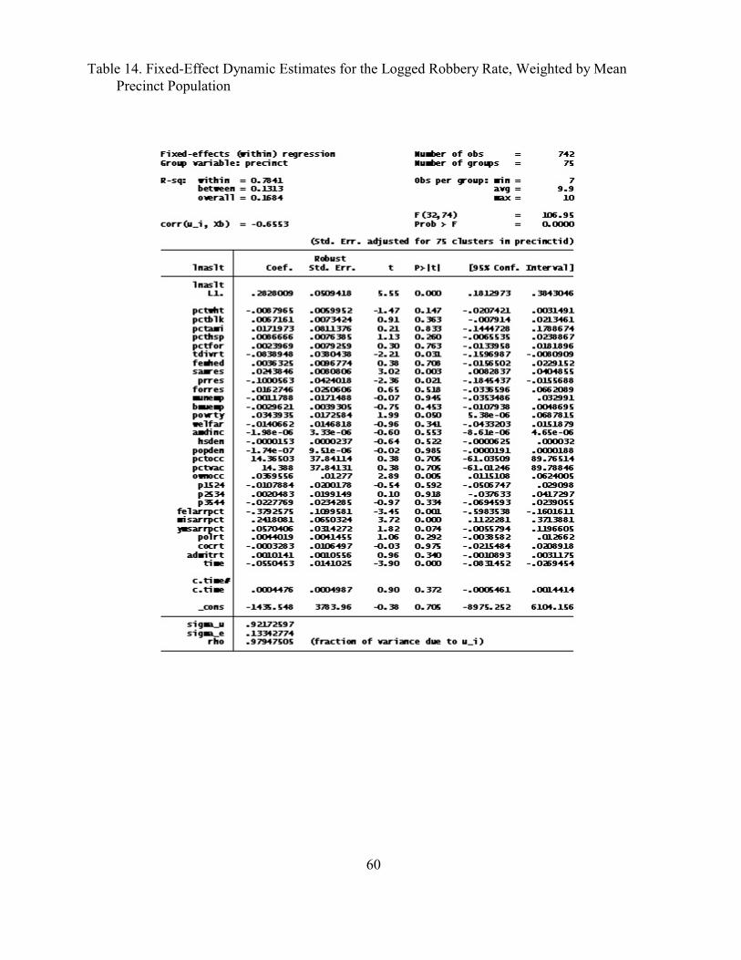
60

Table 14. Fixed-Effect Dynamic Estimates for the Logged Robbery Rate, Weighted by Mean Precinct Population

61

Table 15. Contribution of Four Variables to Change in Logged Homicide Rates

Variable Level, 1988 Level, 2001 Estimated Coefficient Contribution

Poverty 18.80 21.54 .052 .142

Welfare 13.73 16.19 -.058 -.143

Percent 25-34 19.03 16.65 -.085 .202

Felony Arrests .265 .447 -.684 -.124

The “Level” entries represent the mean of precinct values, weighted by precinct population

62

Table 16. “Crime Causes Crime” Dynamic Fixed Effects Model for Logged Homicide Rates

63

Table 17. Poisson Regression for Robbery Counts (with Over-dispersion)

Panel A. Tau Matrix (as correlations)

INTRCPT1, P0 1 -.180 -..105 YEAR,P1 -.180 1 -.753 YEAR2, P2 -.105 -.753 1

Panel B. Reliability Estimates for Random Level-1 Estimates

Random Level-1 Coefficient Reliability Estimate

INTRCPT1, PO .881 YEAR, P1 .501 YEAR2, P6 .548

Panel C. Final Estimation of Variance Components

Random Effect Standard Variance df Chi-square P-value Deviation Component___________________________________

INTRCPT1, R0 .760 .578 396 48499.587 .000YEAR SLOPE, R1 .064 .004 396 2319.467 .000YEAR2 SLOPE R2 .005 .000 396 2614.114 .000Level-1 E 4.778 22.82734

64

(Table 17 continued)

Panel D. Final Estimation of Fixed Effects (with robust standard errors)

Standard Approx. Fixed Effect Coefficient Error T-ratio d.f. P-value

For I NTRCTP1, PO INTRCPT2, B00 -5.672 1.209 -4.691 396 .000 UNEMPRT, B01 .054 .005 10.868 5976 .000 PERBLACK, B02 .057 .004 14.755 5976 .000 PERMALE, B03 -.046 .027 -1.694 5976 .000 PER1534, B04 - .001 .009 -.165 4976 .869 REGIONS, B05 -.064 .114 -.561 396 .575 REGIONW, B06 .566 .130 4.365 396 .000 REGIONMW, B07 -.138 .111 -1.251 396 .212For YEAR slope, P1 (×100) INTRCPT2, B10 .25.276 20.789 1.216 396 .225 UNEMPRT, b11 -.293 .001 -2.183 5976 .029 PERBLACK, B12 .196 .405 4.825 5976 .000 PERMALE, B13 -.098 .448 -.219 5976 .827 PER1534, B14 -.521 .111 -4.782 5976 .000 REGIONS, B15 4.159 20.789 1.268 396 .001 REGIONW, B16 2.679 1.563 1.714 396 .087 REGIONMW, B17 4.971 1.351 3.681 396 .000For YEAR2 slope, P2 (×1000) INTERCPT2, B20 -12.812 15.553 -.824 396 .411 UNEMPRT, B21 -.224 .098 -2.285 5976 .029 PERBLACK, B22 -.185 .028 -6.639 5976 .000 PERMALE, B23 -.053 .323 -.165 5976 .869 PER1534 .451 .071 6.326 5976 .000 REGIONS, B25 -1.885 .945 -1.995 396 .046 REGIONW, B26 -1.207 1.171 -1.031 396 .304 REGIONMW, B27 -4.946 1.011 -4.894 396 .000

65

Figure 1. Histogram of slopes in regression of logged homicide rate against time.

66

Figure 2. Histogram of slopes in regression of logged robbery rate against time

67

Figure 3. Histogram of Slopes in regression of logged assault rate against time