ISA Transactions 52 (2013) 662–671

Contents lists available at ScienceDirect

ISA Transactions

0019-05http://d

n CorrE-m

rodrigo.antoni.g

journal homepage: www.elsevier.com/locate/isatrans

Research Article

New validation algorithm for data association in SLAM

Edmundo Guerra a, Rodrigo Munguia b, Yolanda Bolea a, Antoni Grau a,n

a Automatic Control Department, Technical University of Catalonia, 5 Pau Gargallo St, 08028 Barcelona, Spainb Departament of Computer Science, CUCEI, Universidad de Guadalajara, 44430 Guadalajara, Mexico

a r t i c l e i n f o

Article history:Received 23 November 2012Received in revised form9 April 2013Accepted 25 April 2013Available online 20 May 2013This paper was recommended for publica-tion by Jeff Pieper

Keywords:Monocular SLAMRoboticsOnly-bearing sensorData association

78/$ - see front matter & 2013 ISA. Publishedx.doi.org/10.1016/j.isatra.2013.04.008

esponding author. Tel.: +34 93 4016975; fax:ail addresses: edmundo.guerra@upc.edu (E. Gmunguia@upc.edu (R. Munguia), yolanda.bolerau@upc.edu (A. Grau).

a b s t r a c t

In this work, a novel data validation algorithm for a single-camera SLAM system is introduced. A 6-degree-of-freedom monocular SLAM method based on the delayed inverse-depth (DI-D) featureinitialization is used as a benchmark. This SLAM methodology has been improved with the introductionof the proposed data association batch validation technique, the highest order hypothesis compatibilitytest, HOHCT. This new algorithm is based on the evaluation of statistically compatible hypotheses, and asearch algorithm designed to exploit the characteristics of delayed inverse-depth technique. In order toshow the capabilities of the proposed technique, experimental tests have been compared with classicalmethods. The results of the proposed technique outperformed the results of the classical approaches.

& 2013 ISA. Published by Elsevier Ltd. All rights reserved.

1. Introduction

The simultaneous localization and mapping (SLAM) is a well-known problem in the robotics community, being one of its mostactive fields of research. SLAM problem states how a mobile robotcan operate in an unknown environment by means of onlyonboard sensors to build a map of its surroundings and how touse it to simultaneously navigate through the environment. Thus,SLAM is one of the most important problems to solve in robotics inorder to build truly autonomous mobile robots. There exist manytechniques and algorithms developed to address this problemrunning on-line in a robotic device. Most of these solutions focuson the estimation of self-mapped features detected by sensors. Themost frequently used sensors in SLAM techniques includeodometers, radar, GPS, and several kinds of range finders such aslaser, sonar and infrared-based sensors [1,2].

All these sensors have their own advantages, but several draw-backs must be considered. A common feature of range finders is thecomplex, time consuming algorithms to solve data association.Besides, most of the range finder sensors will produce only 2Dinformation, thus additional sensors are required to know the fullpose of the system to estimate the height, such as GPS and thepreviously mentioned odometers. GPS is a reliable sensor only as far

by Elsevier Ltd. All rights reserved

+34 93 4017045.uerra),a@upc.edu (Y. Bolea),

as it can guarantee the reception of signals from multiple satellites,and therefore it is unable to operate for experimentation in manyenvironments. On the other side, odometers usually provide moreaccurate orientation data autonomously, and can be used to trackfull pose through dead reckoning, but they tend to suffer fromgreatly drift. Thus, SLAM techniques based on range finder willrequire a more complex system introducing additional sensors forpose estimation. At the same time, consumer demand has pushedindustry towards a mass production of cheap and reliable cameradevices at relatively low prices. All these factors have contributed tothe appearance of recent works around the use of cameras as mainsensors. The requirements of accessibility and easiness associatedwith the use of cameras, and the amount and diversity of the dataprovided by them as sensors, make computer vision an obviouschoice in order to streamline autonomous robotics.

The use of a camera as the main sensor within SLAM context isof interest by the information it is able to provide. Computer visionresearch is constantly developing techniques to obtain informationfrom images that can be used in visual SLAM. Anyway, monocularSLAM with 6 degrees of freedom (as presented in this work)remains one of the hardest SLAM variants because only-bearingdata is provided by the camera, and thus especial techniques areneeded to obtain information about the depth of a given point inan image. This problem has several solutions within the structure-from-motion field of research [3,4]. These solutions, although theyare closely related to monocular SLAM, rely on global nonlinearoptimization methods, making them unsuitable for the lesspowerful systems.

.

Nomenclature

Scalars

sV linear speed variancesΩ angular speed variancexi, yi, zi camera coordinatesθi,ϕi camera azimuth and elevationri real depth to featureρi inverse depth to featureaW linear speed covarianceαW angular speed covarianceαmin minimum parallax anglebmin minimum baseline distanceud, vd image point coordinatessu,sv image noise variancesD2H Mahalanobis distance for hypothesis H

Χ2d, τ Chi-squared distribution

hnHOHCT terminal nodes visited by HOHCT algorithm

hnJCBB terminal nodes visited by JCBB algorithm

Vector

x augmented state vectorxv robot camera state vectorrWC camera optical center position quaternion

qWC robot camera orientation quaternionνW robot camera linear speed vectorωW robot camera angular speed vectoryi feature i vectorfv camera motion prediction modelυW linear speed pulse assumed by modelζW angular speed pulse assumed by modelhc measurement prediction modelg Kalman innovation vectorz features measurement vectorh predicted features vectorgH Kalman innovation for hypothesis

Matrix

Q process noise matrix∇Fu process noise Jacobian matrixRCW world to camera transformation matrix∇Hi measurement model Jacobian matrixS innovation covariance matrixRuv measurement noise matrixW Kalman gain matrixP augmented state covariance matrix∇Fx stated prediction model Jacobian matrixSH innovation covariance matrix for hypothesis H

E. Guerra et al. / ISA Transactions 52 (2013) 662–671 663

Some relevant works on monocular SLAM rely on additionalsensors. In [5], mixing inertial sensors with a camera into aniterated extended Kalman filter (IEKF) is proposed. Other authorshave studied extensively different estimation and filtering techni-ques, such as particle filters (PF) [6], sum of Gaussians [7] andmultiple hypotheses filters [8]. Still, some of the most notableworks are based on the well-known extended Kalman filter EKF:Davison [9] proved the feasibility of real-time monocular SLAMwithin EKF; and Montiel [10] developed the inverse-depth I-Dparameterization, which allows initializing features when they areseen by the robot with a heuristically chosen value for depth.

Within the monocular SLAM problem, the batch validationproblem has been considered only since recent years. A goodsurvey of techniques can be found in [11]. Early implementationsof SLAM techniques dealt with each data association individuallybut this validation strategy frequently leads to unreliable results,as it is easy to have a wrong match due to environment textureand geometry. Eventually batch validation was introduced, con-sidering multiple data associations to be validated at the sametime. Currently several tests and methodologies exist to deal withbatch validation of data association. One of the most usualvalidation methods is the joint compatibility branch and boundtechnique, JCBB [12]. This method is considered a strong batchvalidation technique but the algorithm has in its worst case anexponential cost, partly mitigated by several optimizations. Thismethod shows great results within the context of undelayed depthfeature initialization, as it allows ignoring those deemed incom-patible matches with the rest of data association pairs, testing anestimation of the Mahalanobis distance of the innovation. Thisdistance is used to deal with data association but some ambi-guities are produced requiring the development of more sophis-ticated methods, such as Kwok et al. [13], where the authorspropose the utilization of cost functions, enhancing robustnessand assuring performance of a bearing-only SLAM methodology.Another widely known batch validation technique is the combinedconstraint data association (CCDA) by Bailey [14], based on graphs

instead of trees. The technique strengths reside in the ability totest batch validation without knowing the device pose robustly incluttered environments. Latest trends include the utilization ofrandom sample consensus (RANSAC) techniques, such as the 1-point RANSAC [15,16].

This work presents a novel algorithm (HOHCT) to address thedata association validation problem in a Monocular SLAM frame-work based on the delayed inverse-depth initialization (DI-D)technique but it can be applied to another point feature SLAMapproaches. The DI-D method is widely explained and tested in aseries of previous authors' works [17,18,22] which still presentedsome weak points regarding the data association in certain cases,because no data validation technique was featured. In these paperssome important aspects such as parameter tuning, loop-closure,applied to large environments, and a comparison with othermethods are covered in detail, wheresa this work focuses on theHOHCT applied to DI-D as data validation technique. The experi-mental results with real data show that the performance of the DI-D method is clearly improved with the inclusion of the HOHCTvalidation test. Moreover, compared with the JCBB, the proposedmethod outperforms it more efficiently in terms ofcomputational cost.

2. Monocular SLAM with DI-D initialization

The following section describes the procedure to perform themonocular SLAM technique, as shown in Algorithm 1. The descrip-tion of the proposed methodology is based on terms of processesthrough pseudocode and deals with mathematical aspects throughformulation.

x¼ ½xv; y1;…yn�T ð1Þ

xv ¼ rWC qWC vW ωWh iT

ð2Þ

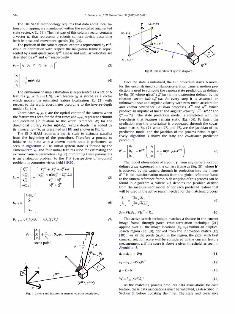
Fig. 2. Initialization of system diagram.

E. Guerra et al. / ISA Transactions 52 (2013) 662–671664

The EKF SLAM methodology requires that data about localiza-tion and mapping are maintained within the so-called augmentedstate vector, x(Eq. (1)). The first part of this column vector containsa vector xv that represents a robotic camera device, describingboth its pose and movement speeds (Eq. (2)).

The position of the camera optical center is represented by rWC,while its orientation with respect the navigation frame is repre-sented by a unit quaternion qWC. Linear and angular velocities aredescribed by νW and ωW respectively.

yi ¼ xi yi zi θi ϕi ρih iT

ð3Þ

xiyizi

264

375þ 1

ρimðθi;ϕiÞ ð4Þ

The environment map estimation is represented as a set of Nfeatures yi, with i¼[1..N]. Each feature yi is stored as a vectorwhich models the estimated feature localization (Eq. (3)) withrespect to the world coordinates according to the inverse-depthmodel (Eq. (4)).

Coordinates xi, yi, zi are the optical center of the camera whenthe feature was seen for the first time; and θi,ϕi, represent azimuthand elevation (in relation to the world reference W) for thedirectional unitary vector m(θi,ϕi). Feature depth ri is coded byits inverse: ρi¼1/ri as presented in [10] and shown in Fig. 1.

The DI-D SLAM requires a metric scale to estimate parallaxfrom the beginning of the procedure. Therefore a process toinitialize the state with a known metric scale is performed, asseen in Algorithm 2. The initial system state is formed by thecamera-state xv, and four initial features used for estimating theextrinsic camera parameters (Fig. 2). Computing these parametersis an analogous problem to the PnP (perspective of n-points)problem in computer vision field [19,20].

f v ¼

rWCkþ1

qWCkþ1

vWkþ1

ωWkþ1

2666664

3777775¼

rWCk þ ðvWk þ υW

k ÞΔtqWCkþ1 � qððωW

k þ ζWk ÞΔtÞvWk þ υW

k

ωWk þ ζWk

2666664

3777775 ð5Þ

xkþ1 ¼

f vðxvÞy1⋮yn

266664

377775 ð6Þ

Pkþ1 ¼∇FxPk∇FxT þ∇FuQ∇FuT ð7Þ

Fig. 1. Camera and features in augmented state description.

Once the state is initialized, the EKF procedure starts. A modelfor the unconstrained constant-acceleration camera motion pre-diction is used to compute the camera state prediction, as definedby Eq. (5) where q((ωW

k +ζWk )Δt) is the quaternion defined by therotation vector (ωW

k +ζWk )Δt. At every step it is assumed anunknown linear and angular velocity with zero-mean accelerationand known covariance Gaussian processes, aW and αW, whichproduce an impulse of linear and angular velocity: υW¼aWΔt andζW¼αWΔt. The state prediction model is completed with thehypothesis that features remain static (Eq. (6)). To finish theprediction step the uncertainty is propagated through the covar-iance matrix, Eq. (7), where ∇Fx and ∇Fu are the Jacobian of theprediction model and the Jacobian of the process noise, respec-tively. Algorithm 3 shows the state and covariance predictionprocedure.

hc ¼hx

hyhz

264

375¼ RCW

xiyizi

264

375þ 1

ρimðθi;ϕiÞ−rWC

0B@

1CA ð8Þ

The model observation of a point yi from any camera locationdefines a ray expressed in the camera frame as (Eq. (8)) where hC

is observed by the camera through its projection into the image.RCW is the transformation matrix from the global reference frameto the camera reference frame. A description of this process can befound in Algorithm 4, where ∇Hi denotes the Jacobian derivedfrom the measurement model hC for each predicted feature thatwill be used in the active search needed for the matching process.

SxSy

" #¼

2nffiffiffiffiffiffiffiffiffiffiffiSið1;1Þ

p2n

ffiffiffiffiffiffiffiffiffiffiffiSið2;2Þ

p" #

ð9Þ

Si ¼∇HiPkþ1∇HiT þ Ruv ð10Þ

This active search technique matches a feature in the currentimage frame through patch cross-correlation technique [21],applied over all the image locations (ud, vd) within an ellipticalsearch region (Eq. (9)) derived from the innovation matrix (Eq.(10)). For all the pixels (ud,vd) in the region, the pixel with bestcross-correlation score will be considered as the current featuremeasurement zi if the score is above a given threshold, as seen inAlgorithm 5.

xk ¼ xkþ1 þWg ð11Þ

Pk ¼ Pkþ1−WSiWT ð12Þ

g¼ zi−hi ð13Þ

W ¼ Pkþ1∇HTi S

−1i ð14Þ

As the matching process produces data associations for eachfeature, these data associations must be validated, as described inSection 3, before updating the filter. The state and covariance

E. Guerra et al. / ISA Transactions 52 (2013) 662–671 665

update equations follow classical EKF formulation (Eqs. (11)–(14)).This process is described in Algorithm 6.

To add features to the state, the DI-D feature initialization isused, [17]. Based on stochastic triangulation, a hypothesis of aninitial feature depth using a delay is defined (Fig. 3). The initializa-tion process can be summarized in a few steps, as shown inAlgorithm 7:

�

When a feature is detected for the first time k, featureinformation, current state xk and covariance Pk are stored.These data are called candidate points λ.

�

In subsequent instants k+dt, the parallax α is estimated using:(i) the base-line, (ii) the associated data λ, and (iii) the currentstate x.

�

If a minimum parallax threshold αmin is reached, the candidatepoint is initialized as a new feature ynew . The new covariancematrix P is fully estimated by the initialization process.

3. Highest order hypothesis compatibility test

Delayed inverse-depth (DI-D) initialization uses an activesearch technique to address the problem of data association. Evenwith a correct matching data association errors may be present: amoving object can be correctly matched but it can give a landmarkinformation which disrupts the map, as this ‘fake’ landmark is notstatic. Other errors may arise when dealing with ambiguoustextures and features on the mapped environment, producingincorrect matching due reflections, repeated designs, compositelandmarks, etc.

The proposed algorithm, HOHCT, exploits the fact that delayedinitialization implementations for monocular SLAM are morerobust to data association errors. This robustness comes from thefact that candidate features must satisfy a series of tests andconditions before being considered as suitable landmarks to beinitialized. In the context of the implemented DI-D [17], a featuremust be tracked correctly within a minimal number of frames andit has to achieve a parallax value greater than a minimum αmin toguarantee accurate depth estimation, see [22]. These conditionsallow the DI-D monocular SLAM to reject most of the weak and/orincorrectly matched features. Still, data association errors canhappen sparsely, so the technique works on the optimistic hypoth-esis that most of the time the number of incorrect data association

Fig. 3. Diagram of parallax α estimation.

pairs will be low. The data validation test presented is based on acomparison of a quality metric against a statistical threshold ofacceptance, like in JCBB [12,23]. So, the tested data associationpairs are valid or invalid as a whole set, being jointly consistent orcompatible.

D2Η ¼ gT

ΗS−1iΗ gΗ≤χ

2d;τ ð15Þ

So, this compatibility test evaluates hypotheses, where eachhypothesis is a subset of the data association pairs obtained fromthe matching process. The pairs of each subset are tested togetherto find whether they form a compatible hypothesis or not. Todetermine the compatibility of a hypothesis the Mahalanobisdistance is estimated (Eq. (15)). This distance is used as a qualitymetric tested against a threshold given by the Chi-squareddistribution, [12,23,24], where χ2d,τ is the Chi-squared distributionwith a default confidence level of τ, and d is the number of dataassociation pairs accepted into the hypothesis. The distance itselfis estimated from gH and SiH, which are the innovation andinnovation covariance for the hypothesis respectively, computedin the update and matching steps of EKF, in Eq. (13) and Eq. (10).Not all the data association pairs are taken into account in eachhypothesis, so only relevant rows and columns of gH and SiH willbe considered.

In DI-D monocular SLAM each mapped landmark is associatedwith a unique feature of the image, so the mentioned hypothesiscan be represented as an array of Boolean values, where each pairis accepted or rejected. An example of pair rejection after theHOHCT application can be seen in Fig. 4. Initially an optimistichypothesis taking all pairs is tested. If this hypothesis fails to passthe compatibility test, a search for a satisfactory hypothesis isperformed. While a vector of Boolean values has to be found, arecursive exploration on a binary tree could be too cumbersome,as it generally involves traversing excessive nodes, even withpruning, which in turn represents an increase of the computa-tional complexity. Thus, unlike JCBB, an approach combiningiteration and recursion is taken, shown in Algorithm 8. For a givenset of data association pairs, the hybrid recursive/iterative part ofthe algorithm searches a hypothesis which has an exact number ofcompatible pairs. This search will be performed iteratively, con-sidering at each step a decreasing number of compatible pairs. So,on the first performed search, the hypothesis that all the pairs areconsidered compatible except one will be searched. If this searchdoes not find any compatible hypothesis, a new search for ahypothesis with all the pairs deemed compatible except two willbe performed. Thus, as seen in Algorithm 8, when the search fails,the number of pairs to be rejected (represented by index ‘i’) fromthe full set of pairs (containing ‘m’ data association pairs) isincremented by 1, until a compatible hypothesis is found. At thispoint the hypothesis contains ‘m−i’ compatible data pairs, and only‘i’ rejected pairs.

The loop in the HOHCT-test function in Algorithm 8 maintainsthe accounting for failed searches, increasing the index ‘i’ and

Fig. 4. Example: pair elimination and hypothesis formation.

Fig. 5. Example of search with m¼4 with increasing number of pairs to be rejected generating different trees.

Fig. 6. Environment used for tests.

E. Guerra et al. / ISA Transactions 52 (2013) 662–671666

performing new searches. Each call to HOHCT-Rec function fromHOHCT-test function starts a new search where a tree is explored.In this exploration the accepted pairs in the hypothesis areindicated with ‘1’, being introduced by the iterative part of thefunction; on the other hand rejected pairs (indicated as ‘0’) areintroduced by the recursive part of the function. This allowsmaking a search into an optimized binary subtree where onlythe interesting nodes (those having exactly ‘m−i’ accepted pairs)will be tested for joint compatibility.

In Fig. 5 the different trees that could be considered arerepresented. Tree 1 represents the first set of hypotheses that willbe used to calculate the distance between pairs. If there are nocompatible hypotheses (if the statistical test fails) then Tree 2 isbuilt and the compatibility is checked again; this process of treecreation is iteratively repeated until a compatible hypothesisis found.

Given the sparse error conditions found in the DI-D initializa-tion SLAM, this ordered search will have normally a linear costwith the number of matched landmarks, with exceptional casesachieving cubic cost in some specific frames, still very far from theexponential cost that binary tree recursion could represent overthe whole number of matched landmarks. In this work, therejected landmarks are eliminated just as deemed incompatible.

4. Experimental results and discussion

In order to test the performance of the proposed method,several video sequences were acquired using a low cost camera.Then, a prototype implementation in C++ of the algorithm wasexecuted off-line using those video sequences as input signals. Inthe experiments, several parameter values were used: variancesfor linear and angular velocity respectively sV¼4(m/s)2, sΩ¼4(m/s)2, noise variances su¼sv¼1 pixel, minimum base-linebmin¼15 cm and minimum parallax angle αmin¼51. These valueshave been adjusted heuristically, according to criteria described in[22]. Regarding the values in [22], the parameters αmin, sV and sΩhave increased their value to deal with greater uncertainty fromsample to sample, introduced by a lower frame rate (from 30 to15 fps), as discussed below. As such, the base-line bmin wasincreased to guarantee the new minimum parallax needed tocompute an initial estimation of feature depth. The default con-fidence level for the Chi-squared distribution in the HOHCT wasset to τ¼0.95.

A Logitech C920 HD camera was used in experiments. This lowcost camera has an USB interface and wide angle lens, acquiringHD color video. However, in experiments, grey level videosequences, with a resolution of 424�240 pixels captured at 15

frames/s, were used. This low image resolution is widely used inorder to achieve approximated real-time SLAM algorithms. Lowerresolutions like 320�240 pixels are also used in several worksproducing good results, [15,23]. While a camera with a higherframe rate would probably led to better trajectory estimationresults, higher resolutions are rarely used in SLAM context as theimage processing costs grow rapidly, without improving propor-tionally the effectiveness of the algorithm.

The video sequences have been acquired inside the Vision andIntelligent Systems laboratory, where a rail guide is assembled inorder to provide an approximate ground truth reference, see Fig. 6.Every video sequence has been acquired sliding the camera(manually), at different speeds, along the rail guide. The durationof the different sequences runs from 35 s to 1 min, for a total of7350 frames accumulated over the different sequences.

Fig. 7 illustrates some examples of factors inducing dataassociations deemed incompatible. The star shaped marks areenveloping the area where incompatible data associations lay andare ignored. Blue and red crosses are signaling points of interestwhere landmark candidates lay for the DI-D and points of interestbeing tracked to estimate their parallax. Green crosses are signal-ing the observed landmarks, and the small red circumferences arecentered on the predicted point features. Although some of theincompatibilities are small, the accumulated effect of the inducederror over several frames and the relative size of the landmark setcan produce intense dampening effect on map estimation.

Fig. 8 illustrates the estimated map and trajectory for fourdifferent video sequences. The left and right columns show theresults for each sequence, with and without HOHCT data valida-tion. It is important to note that all the video sequences have beenacquired at a relatively low frame rate of 15 frames/s instead of thestandard minimum of 25–30 frames/s on most monocular SLAM

Fig. 7. (a) Incompatibility due repeated design. (b) Incompatibility found at composite landmark. (c) Incompatibilities produced by reflections on materials and curvedsurfaces. (For interpretation of the references to color in this figure, the reader is referred to the web version of this article.)

E. Guerra et al. / ISA Transactions 52 (2013) 662–671 667

experiments, thus making the SLAM process harder. As it could beexpected, the estimations obtained with the HOHCT validationwere consistently better. In this case the experimental resultsshow that HOHCT validation test significantly improves the algo-rithm robustness, by rejecting harmful matches. An importantimprovement that was commonly observed is the enhancedpreservation of the metric scale on estimations. Also, as it mightbe expected, video sequences that were acquired moving thecamera in a slow fashion offer more coherent results due to thelow frame rate.

To test the local reliability of the proposed approach, sub-mapping techniques were not considered, as they would difficultthe metric scale estimation propagation. As keeping into the stateall the observed features produces an excessive growth of compu-tational costs in the SLAM framework, a visual odometry strategywas adopted. Thus, older features, considering their ‘age’ as thetime since they were last observed, are removed in order tomaintain a stable number of features, and therefore stabilizingthe computational cost per frame. This characteristic makesprevious mapped areas unrecognizable for the SLAM algorithmitself but alleviates the computational cost while maintaining lowtrajectory drift, as seen in Fig. 8.

However, in the context of visual odometry, this fact is notconsidered as a problem. A modified monocular SLAM methodthat maintains the computational operation stable can be viewedas a complex real-time virtual sensor, which provides appearance-based sensing and emulates typical sensors such as a laser forrange measurements and encoders for dead reckoning (visualodometry).

In authors' related work [17] the virtual sensor idea is pro-posed, developed, and extended so that, using a distributedscheme, it is possible to recognize previous mapped areas for loopclosing tasks. In this scheme, the outputs provided by the virtualsensor have been used by an additional SLAM process (decoupledfrom the camera's frame rate) in order to build and to maintain theglobal map and final camera pose. This present work considers theapproach of monocular SLAM as a virtual sensor.

hHOHCTn ¼ ∑r

i ¼ 1ni ð16Þ

hnJCBB ¼ 2n− ∑

r

i ¼ 12n−i ð17Þ

The benefits of the application of the HOHCT validation comestogether with the addition of the computational cost of exploring atree with hn

HOHCT leaf nodes and testing them against the Maha-lanobis distance. In Eq. (16), n is the number of landmarksobserved and r the quantity of these observations deemed incom-patible at the optimal hypothesis. Thus the number of hypothesisto explore defines the order of the cost (the Mahalanobis distancefor each hypothesis is efficiently computed according to Eq. (15)).Meanwhile, the cost of using JCBB in terms of visited leaf nodes isdescribed in Eq. (17), where n and r are the number of dataassociation pairs and the number of pairs to be rejected at theoptimal hypothesis, respectively. It is well worth to see how thevalue with more relevance in Eq. (17) is the number of data pairs n,on term 2n, which increases the cost exponentially. This exponen-tial cost can be relieved by a high number of rejected data pairs, r.As discussed above, the DI-D tends to produce strong dataassociation pairs with low rejected associations, r, thus makingJCBB to grow near exponential swiftly, because r will rarely growenough to compensate the term 2n.

Still, the theoretical computational cost for the HOHCT test couldbe higher. However, the experimental data show that the HOHCTalgorithm tends to present linear cost when used along with thedelayed feature initialization technique. In Table 1, the resultsobtained in the tests are shown. For a sample of 7350 frames(accumulated over different video sequences) only 22 times (0.3% ofthe cases) the computational cost of the test becomes quadratic. Forthe same sample, the case where r¼3 is never found. The differencein terms of nodes to explore was observed in experimental computa-tional times. Table 2 shows the results obtained in terms of time perframe in milliseconds. Considering that for the experiments slowsequences at 15 fps were used, both approaches reached average real-time performance. It must be noted that the sequences were acquiredmanually but with an artificial ground truth, easing the featuretracking and matching processes, thus improving the performance.Anyway, the average computational time per frame of the DI-D SLAMwith JCBB validation doubled the total time of the DI-D SLAM withHOHCT, and presented a much greater standard deviation. This was

Fig. 8. Map and trajectory estimation results obtained from four video sequences: (a) 845 frames, (b) 675 frames, (c) 615 frames and (d) 750 frames. Left column displaysresults using HOHCT, while right column displays results for the same sequences without using HOHCT batch validation. The units in axes are in centimeters.

E. Guerra et al. / ISA Transactions 52 (2013) 662–671668

due to the fact that worst cases on JCBB, as shown in Eq. (17), are ofnear exponential nature, but not as time consuming as one mightexpect. This is because JCBB can compute matrix inversions incre-mentally in optimal ways. This technique reduces the matrix

inversion cost from cubic to quadratic for iteratively growing matrix(such as those found at the JCBB) after the first matrix is inverted. Thisoptimization hugely reduces the JCBB computational cost, but notenough to fully compensate the size of the search space explored.

Table 1Results of HOHCT failed tests and number of matching deemed incompatible.

Rejected pairs per frame (r) Incidences Relative frequency (%)

r¼2 (incompatible) 22 0.3r¼1 (incompatible) 234 3.18r¼0 (compatible) 7094 96.52Total 7350 100

Table 2Average computation time per frame for the DI-D Monocular SLAM with JCBB andHOHCT validations

Average time per frame (ms) Standard deviation

JCBB 52.73 19.20HOHCT 24.31 2.62

E. Guerra et al. / ISA Transactions 52 (2013) 662–671 669

5. Conclusions

The main contribution of this paper is to present a novelalgorithm (HOHCT) for addressing the problem of batch validationof data association in the context of monocular SLAM. HOHCTevaluates the compatibility of a given set of matches of visualfeatures, and tries to obtain the largest subset of compatiblematches efficiently. Although HOHCT is derived in order to exploitsome of the characteristics of the delayed inverse-depth (DI-D)monocular SLAM method, it can be easily applied to othermonocular SLAM approaches. The main feature exploited is thelow rate of spurious data association pair produced by the DI-Dframework.

In DI-D, landmarks are only introduced into the EKF once theavailable depth estimation is accurate enough. This leads to theintroduction of fewer landmarks into the EKF but with moreaccuracy than the un-delayed approaches. Still a data associationgating technique is needed, so a batch validation technique basedon statistical thresholding is introduced. This technique, the high-est order hypothesis compatibility test HOHCT, has been shown toimprove greatly the monocular SLAM results on certain circum-stances. These circumstances include emergence of ‘false’ land-marks, difficult illumination conditions, and irregular trajectorieswith non-smooth changes on linear or angular velocities. Addi-tionally, tests show that the algorithm responsible for finding thebest hypothesis when the batch validation test fails will rarely gobeyond quadratic cost with respect to the set of observed features,in fact being more prone to linear cost, though having anexponential worst case scenario. This fact allows to produce a firstprototype of a DI-D Monocular SLAM framework with HOHCTvalidation which demonstrates to be able to reach real timeperformance for the studied cases, under 15 fps assumption.

Algorithms

Algorithm 1. DI-D SLAM with HOHCT.

Procedure DI-D SLAM with HOHTC (x0, P0, vid, refini)Input:x0 initial state for the robotic cameraP0 initial state covariancevid sequential image videorefini initial reference pointsbeginimgref:¼vid.FirstFrame()

k:¼1;(xk, Pk):¼ Initialize (imgref, refini)while true doimg:¼vid.NextFrame()(xk+1, Pk+1):¼StatePrediction (xk, Pk)(hi, ∇Hi):¼MeasurementPrediction (xk+1, Pk+1)(zi, Si):¼Matching (hi, ∇Hi,Pk+1,img)(hi, zi,∇Hi, Si):¼HOHCT-test (hi, zi, ∇Hi,, Si)(xk, Pk):¼Update (xk+1, Pk+1, hi, zi, Si)(xk, Pk):¼AddFeatures(xk, Pk, img)k:¼k+1;

end whileend

Algorithm 2. Metric scale and system initialization.

Function (xk, Pk):¼ Initialize (img, refini)Input:img image from sequencerefini coordinates of initial points on screenOutput:xk initial state for the robotic cameraPk initial state covariancebegincompute 4-points PnP with refini datafor each point ‘i’ in refini dosave image patch around point refini[i]update xk with data from feature ‘i’update Pk with data from feature ‘i’

end forreturn (xk, Pk)

Algorithm 3. State and covariance prediction.

Function (xk+1, Pk+1):¼StatePrediction (xk, Pk)Input:xk previous robot state estimationPk previous state covarianceOutput:xk+1 state estimation predictionPk+1 estimation covariancebeginupdate robotic camera state prediction fvcompute state prediction jacobian ∇Fxcompute process noise jacobian ∇Fuupdate state prediction covariance Pk+1

return (xk+1, Pk+1)

Algorithm 4. Measurement prediction and jacobian ∇Hicomputation.

Function (hi, ∇Hi) :¼MeasurementPrediction (xk+1, Pk+1)Input:xk+1 state estimation predictionPk+1 estimation covarianceOutput:hi features observation prediction∇Hi observation Jacobianbeginfor each feature ‘i’ in xk+1 docalculate measurement prediction hi

i

if hii is not NULL thenadd hi

i to hicompute Jacobian ∇Hi

i for hii

add ∇Hii to ∇Hi

end if

E. Guerra et al. / ISA Transactions 52 (2013) 662–671670

end forreturn (hi, ∇Hi)

Algorithm 5. Data association through active search matching.

Function (zi, Si) :¼Matching (hi, ∇Hi, Pk+1, img)Input:Pk+1 estimation covariancehi features observation prediction∇Hi observation Jacobianimg image from sequenceOutput:Si innovation covariance matrixzi matching observations foundbegincalculate RiSi :¼∇Hi Pk+1∇Hi

T+Rifor all predicted observations ‘n’ in hi do

if hi(‘n’) is not NULL thencompute acceptance Region with Si(px,py) :¼NULL;_maxCorrelation :¼0;

for all the points ‘i,j’ in Region dobuild a patchij around ‘i,j’calculate patchij _crossCorrelationif _crossCorrelation4¼_maxCorrelation then(px,py) :¼ ‘i,j’_maxCorrelation :¼_crossCorrelation

end ifend forif_maxCorrelation4_correlationThreshold thenadd ‘i,j’ to zi

end ifend if

end forreturn (zi, Si)

Algorithm 6. Update step of the Extended Kalman Filter.

Function(xk, Pk) :¼Update (xk+1, Pk+1, hi, zi, Si)Input:zi matching observations foundxk+1 state estimation prediction from previous statePk+1 estimation covariancehi features observation predictionSi innovation covariance matrixOutput:xk updated state estimationPk updated covariance matrixbegincompute innovation gupdate measurement model jacobian ∇Hi

if HOHCT failed thenupdate innovation covariance matrix Si

end ifcompute Kalman gain matrix Wupdate state estimation and covariance, (xk ,Pk)return (xk, Pk)

Algorithm 7. Process to add features automatically.

Function (xk, Pk) :¼AddFeatures(xk, Pk, img)Input:img image from sequencexk updated state estimationPk updated covariance matrix

Output:xk updated state estimationPk updated covariance matrixbegin_activeFeat:¼Number of mapped features on frame_activeCandidate :¼number of candidates from database

seen on frameif (_activeFeat +_activeCandidateoMinFeatOnScreen) thendetect more candidatesadd new candidates to candidate Database

end iftrack features on candidates Database between framesfor each candidate ‘i’ in candidates Database doif candidate ‘i’ has enough parallax then

add feature ‘i’ to state and covariance (xk, Pk)end if

end forreturn (xk, Pk)

Algorithm 8. HOHCT test and algorithm.

Function (hi, zi, Si,∇Hi) :¼HOHCT-test (hi, zi,∇Hi, Si)Input:zi matching observations foundhi features observation predictionSi innovation covariance matrix∇Hi observation JacobianOutput:zi matching observations foundhi features observation predictionSi innovation covariance matrix∇Hi observation Jacobianbeginm: ¼Number of Matches in zihyp :¼[1] m // Grab all matchesif � JointCompatible( hyp, hi,zi, ∇Hi,Si) theni :¼1while iom do // Hypothesis reducer loop(hyp,d2) :¼ HOHCT-Rec(m,0,[],i,hi, zi,∇Hi,Si)If JointCompatible(hyp,hi, zi,∇Hi,Si) then

i :¼melse

i :¼ i+1end ifend whileremove incompatible pairings from hi and ziupdate jacobian ∇Hi and matrix Siend ifreturn (hi, zi, Si,∇Hi)Function (hypb, d2b) :¼ HOHCT-Rec (m, mhyp, hyps, rm, hi,zi,∇Hi,Si)Input:m size of full hypothesismhyp size previously formed hypothesishyps hypothesis built through recursionrm matches yet to removeOutput:hypb best hypothesis found from hyps

d2b best Mahalanobis distancebeginif (rm¼0) or (m¼mhyp) thenhypb:¼[mhyp [1]m−mhyp]d2b :¼Mahalanobis (hi, zi,∇Hi , Si)

elsehypb:¼[hyps[1]m-mhyp]d2b :¼Mahalanobis(hi, zi, ∇Hi, Si)

E. Guerra et al. / ISA Transactions 52 (2013) 662–671 671

for r:¼(mhyp+1) : (m−rm+1) do(h,d):¼HOHCT-Rec (m, mhyp+1, [hyps0],rm−1,hi,zi, ∇Hi, Si)If (dod2b) thend2b :¼d ; hypb :¼h

end ifhyps:¼[hyps1] ; mhyp:¼mhyp+1

end forend ifreturn (hypb, d2b)

Acknowledgments

This work has been funded by the Spanish Ministry of ScienceProject DPI2010-17112.

References

[1] Teslic L, Skrjanc I, Klancar G. Using a LRF sensor in the Kalman-filtering-basedlocalization of a mobile robot. ISA Transactions 2010;49:145–53.

[2] Vázquez-Martín R, Núñez P, Bandera A, Sandoval F. Curvature-based environ-ment description for robot navigation using laser range sensors. Sensors2009;8:5894–918.

[3] Jin H, Favaro P, Soatto S. A semi-direct approach to structure from motion. TheVisual Computer 2003;19(6):377–94.

[4] Fitzgibbon AW, Zisserman A. Automatic camera recovery for closed or openimage sequences. In: Proceedings of the European Conference on ComputerVision; 1998.

[5] Strelow S, Sanjiv D. Online motion estimation from image and inertialmeasurements. Workshop on Integration of Vision and Inertial SensorsINERVIS; 2003.

[6] Kwok NM, Dissanayake G. Bearing-only SLAM in indoor environments.Australasian Conference on Robotics and Automation; 2003.

[7] Kwok NM, Dissanayake G, Ha QP. Bearing-only SLAM using a SPRT basedGaussian sum filter. In: Proceedings of the IEEE International Conference onRobotics and Automation (ICRA05), Barcelona, Spain; 2005. p. 1121–6.

[8] Kwok NM, Dissanayake G. An efficient multiple hypothesis filter for bearing-only SLAM. In: Proceedings of IEEE/RSJ International Conference on IntelligentRobots and Systems (IROS04), Sendai, Japan, Sep/Oct 2004; 2004. p. 736–41.

[9] Davison A, Gonzalez Y, Kita N. Real-Time 3D SLAM with wide-angle vision.IFAC Symposium on Intelligent Autonomous Vehicles; 2004.

[10] Montiel JMM, Civera J, Davison A. Unified inverse depth parameterization formonocular SLAM. Robotics: Science and Systems Conference; 2006.

[11] Durrant-Whyte H, Bailey T. Simultaneous localization and mapping: part I.IEEE Robotics & Automation Magazine 2006;13:99–106.

[12] Neira J, Tardos JD. Data association in stochastic mapping using the jointcompatibility test. IEEE Transaction on Robotics and Automation 2001;17(6):890–7.

[13] Kwok NM, Ha QP, Fang G. Data association in bearing-only SLAM using a costfunction-based approach. In: Proceedings of the 2007 IEEE InternationalConference on Robotics and Automation (ICRA07), Roma, Italy, April 2007. p.4108–13.

[14] Bailey T. Mobile robot localisation and mapping in extensive outdoor envir-onments. Ph.D. dissertation, University of Sydney, Australian Centre for FieldRobotics; 2002.

[15] Civera J, Grasa OG, Davison AJ, Montiel JMM. 1-point RANSAC for EKF-basedStructure from motion. International Conference on Intelligent Robots andSystems; 2009. p. 3498–504.

[16] Williams B, Smith P, Reid I. Automatic relocalisation for a single-camerasimultaneous localisation and mapping system. International Conference onRobotics and Automation; 2007.

[17] Authors and title hidden for the blinded version. IEEE Transactions onInstrumentation and Measurement 2009;58(8):2377–84.

[18] Authors and title hidden for the blinded version. 17th IFAC World Congress;2008.

[19] Chatterjee C, Roychowdhury V. Algorithms for coplanar camera calibration.Machine Vision and Applications 2000;12:84–97.

[20] Fishler M, Bolles RC. Random sample consensus: a paradigm for model fittingwith applications to image analysis and automated cartography. Communica-tions of ACM 1981;24(6):381–95.

[21] Davison A, Murray D. Mobile robot localisation using active vision. In:Proceedings of the European Conference on Computer Vision; 1998.

[22] Authors and title hidden for the blinded version. Proceedings of the 3rdEuropean Conference on Mobile Robots ECMR, Freiburg Germany; 2007.

[23] Clemente L, Davison A, Reid I, Neira J, Tardós, JD. Mapping large loops with asingle hand-held camera. In: Proceeding of Robotics: Science Systems 2007;June 2007, Atlanta.

[24] David A. Matrix algebra from a statistician's perspective. Springer-Verlag;1998.