New Product DynamicsIllustrative System Dynamics Models

Craig W. KirkwoodArizona State University

Copyright c© 1998, C. W. Kirkwood (version 1b – 12/4/98, 10/8/12)

All rights reserved. No part of this publication can be reproduced, stored in a re-trieval system, or transmitted, in any form or by any means, electronic, mechan-ical, photocopying, recording, or otherwise without the prior written permissionof the copyright holder.

Vensim is a registered trademark of Ventana Systems, Inc.

Contents

1 Total Market Dynamics . . . . . . . . . . . . . . . . . 1

1.1 Infinite Potential Customers 21.2 Finite Potential Customers 41.3 Determining Logistic Model Parameters 71.4 References 111.5 Exercises 11

2 Competitive Market Dynamics . . . . . . . . . . . 13

2.1 Infinite Potential Customers 132.2 Finite Potential Customers 142.3 Bandwagon Markets 152.4 References 19

Preface

These notes provide illustrative examples of models for new product marketdynamics based on “word-of-mouth” modeling concepts. Both differential equa-tion and Vensim system dynamics model notation are presented for these models.A version of Vensim is available free for instructional use over the World WideWeb at www.vensim.com. Further support material related to system dynamicsis available from my web site at www.public.asu.edu/∼kirkwood.

C H A P T E R 1

TotalMarketDynamics

This chapter discusses system dynamics models for the dynamics of a marketfor an innovative durable good. Specifically, the models address the growth ofthe total market for a newly developed product that is purchased once by acustomer. The models presented in this chapter are useful in themselves andform basic building blocks for models of competitive markets presented in thenext chapter.

The models in this chapter take a “contagion” view of the process by whichcustomers purchase a product. The basic idea is that potential customers “catch”the desire to purchase a product from those who have already purchased the prod-uct, and therefore the rate at which the product is purchased depends on 1) howmany customers have already purchased the product, 2) how many potential cus-tomers remain for the product, and 3) how persuasive the current customers arein presenting the virtues of the product when they contact potential customers.

This can also be viewed as a “predator-prey” situation, where those who havepurchased the product are predators on the potential customers (the “prey”) andattempt to convert them to the “purchased” state. (Or you may prefer thinkingof those who have purchased the product as zombies who attempt to convertthe potential customers into the zombie-like state of being actual customers forthe product.) A more neutral term for this type of model is “word-of-mouth,”which carries the implication that positive word-of-mouth from satisfied currentcustomers leads potential customers to make a purchase.

While these images help in remembering the structure the models, the actualsituation for most products is more complex. Word of mouth models providea relatively simple description of the complex process that occurs when a newproduct type is introduced. The customers who have purchased the product maynot literally walk around and attempt to sell the product to potential customers,but the degree of attention paid to a new product by potential customers andthose who communicate with them tends to depend on both the number ofpeople who have bought the product and the number of potential customers.Thus, as the product becomes more widely purchased, it receives more attentionin the trade and general press, and is generally more talked about by potentialcustomers. Hence, word-of-mouth sales models do not necessarily imply thatcurrent customers literally talk directly to potential customers and “make the

2 CHAPTER 1 TOTAL MARKET DYNAMICS

sale.” The communication may be more in the nature of a general “buzz” aboutthe product that is “in the air,” and which makes a potential customer morelikely to purchase the product.

In the final analysis, the usefulness of a model should be judged by its valuein providing insights into a situation, and also by its ability to match empiricaldata. By those criteria, the models in this chapter, while relatively simple, areuseful.

1.1 Infinite Potential Customers

We call those who have already purchased the new product of interest “ActualCustomers” and those who might purchase the product “Potential Customers.”In this section, we consider situations where the population of Potential Cus-tomers for the new product is so much larger than the population of ActualCustomers that the number of Potential Customers remains essentially the sameeven when the number of Actual Customers grows.

The model assumes that for a short period of time ∆t each Actual Customerconverts c∆t Potential Customers into Actual Customers, where c is a posi-tive constant (the “conversion coefficient”) that encodes how effective ActualCustomers are at converting Potential Customers. If at time t there are n(t)Actual Customers, each of which converts c∆t Potential Customers into ActualCustomers during the next ∆t time period, then at time t + ∆t the number ofActual Customers will be n(t + ∆t) = n(t) + n(t)c∆t.

By the usual calculus arguments, this equation can be converted to the dif-ferential equation

dn(t)

dt= cn(t) (1.1)

or the integral equation

n(t) = no +

∫

t

0

cn(τ ) dτ (1.2)

where no is the number of Actual Customers at time t = 0. The solution tothese equations is well known to be the familiar exponential

n(t) = noect, t ≥ 0 (1.3)

The Vensim equivalent of equation 1.2 is shown in Figure 1.1, and the modeloutput displayed in this figure shows the familiar exponential growth pattern forboth the number of Actual Customers and the flow of Potential Customers intoActual Customers.

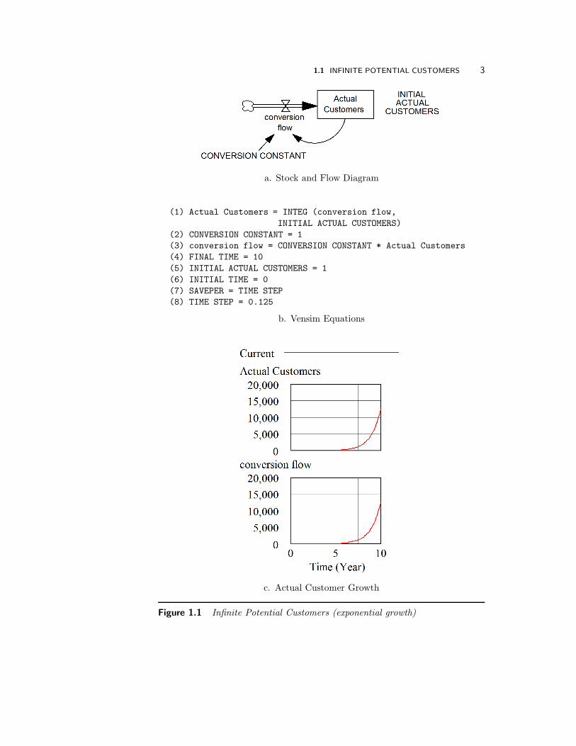
1.1 INFINITE POTENTIAL CUSTOMERS 3

a. Stock and Flow Diagram

(1) Actual Customers = INTEG (conversion flow,

INITIAL ACTUAL CUSTOMERS)

(2) CONVERSION CONSTANT = 1

(3) conversion flow = CONVERSION CONSTANT * Actual Customers

(4) FINAL TIME = 10

(5) INITIAL ACTUAL CUSTOMERS = 1

(6) INITIAL TIME = 0

(7) SAVEPER = TIME STEP

(8) TIME STEP = 0.125

b. Vensim Equations

c. Actual Customer Growth

Figure 1.1 Infinite Potential Customers (exponential growth)

4 CHAPTER 1 TOTAL MARKET DYNAMICS

1.2 Finite Potential Customers

In realistic markets, the exponential growth pattern shown in Figure 1.1 cannotcontinue forever because ultimately all the Potential Customers for a product willbe converted to Actual Customers. This section considers a model that addressesthis reality, and thus develops a model that more closely matches empirical datafor many new product types.

Assume that the total number of Potential Customers for the product is M .Then the total number of remaining Potential Customers at time t is M − n(t),where n(t) is the number of Actual Customers at time t.

Further assume that c represents the conversion rate per Actual Customerwhen there are M Potential Customers. To complete the model specification,we must make an assumption about how the conversion rate for each ActualCustomer changes when the number of Potential Customers drops as they areconverted to Actual Customers. A reasonable assumption to make is that thisconversion rate is linearly proportional to the total number of Potential Cus-tomers who remain at any time. Thus, for example, if half of the PotentialCustomers remain, then the conversion rate for each Actual Customer is c/2,and if a quarter of the Potential Customers remain, then the conversion rate foreach Actual Customer is c/4.

With this assumption, the number of Potential Customers converted by eachActual Customer in a time interval ∆t is {[M − n(t)]/M} × c∆t, and hencethe number of Potential Customers converted by all n(t) Actual Customers isn(t) × {[M − n(t)]/M} × c∆t. By analogous arguments to those used to deriveequation 1.1, these assumptions lead to the differential equation

dn(t)

dt= c ×

M − n(t)

M× n(t) (1.4)

or the equivalent integral equation

n(t) = no +

∫

t

0

c ×M − n(τ )

M× n(τ ) dτ (1.5)

where no is the number of Actual Customers at time t = 0.The solution to equation 1.4 or 1.5 is known to be

n(t) =M

1 + [(M − no)/no]e−ct, t ≥ 0 (1.6)

(Roughgarden 1998). The curves represented by equation 1.6 are called logisticcurves.

The Vensim equivalent of equation 1.5 is shown in Figure 1.2. The curve forActual Customers as a function of time that is shown in Figure 1.2c displays the“s-shaped” pattern that is shown by all logistic growth curves, and the curveshown for conversion flow demonstrates the symmetric bell-shaped curve that isshown by all logistic conversion flows.

1.2 FINITE POTENTIAL CUSTOMERS 5

a. Stock and Flow Diagram

(01) Actual Customers= INTEG (conversion flow,INITIAL ACTUAL CUSTOMERS)

(02) CONVERSION CONSTANT = 1(03) conversion flow = CONVERSION CONSTANT

*(Potential Customers / TOTAL MARKET) * Actual Customers(04) FINAL TIME = 10(05) INITIAL ACTUAL CUSTOMERS = 1(06) INITIAL TIME = 0(07) Potential Customers= INTEG (-conversion flow,

TOTAL MARKET - INITIAL ACTUAL CUSTOMERS)(08) SAVEPER = TIME STEP(09) TIME STEP = 0.125(10) TOTAL MARKET = 100

b. Vensim Equations

c. Actual Customer Growth

Figure 1.2 Finite Potential Customers (logistic growth)

6 CHAPTER 1 TOTAL MARKET DYNAMICS

Properties of Logistic Curves

While this is not obvious from a casual inspection, equation 1.6 reduces toequation 1.3 in the limit as M becomes very large, and equation 1.6 is alsoapproximately equal to equation 1.3 when n(t) is much less than M . Thesefacts can be shown by multiplying the top and bottom of equation 1.6 each by[no/(M − no)]e

ct to yield

n(t) =M × [no/(M − no)]e

ct

[no/(M − no)]ect + 1. (1.7)

For sufficiently small t and/or sufficiently large M , the first term in the denom-inator of equation 1.7 will be much less than 1, and hence the denominator willreduce to approximately 1. In the numerator, M/(M−no) will be approximately1, and hence equation 1.7 will reduce to equation 1.3.

The practical implication of these facts is that when the number of ActualCustomers is much less than the number of Potential Customers, logistic growthappears to be just the same as exponential growth. However, there is a limit outthere somewhere in the future!

The rate at which the number of Actual Customers grows is given by thederivative of n(t), and the time tmax at which this is a maximum can be foundby taking the derivative of the growth rate [that is, the second derivative of n(t)]and setting this equal to zero. The arithmetic is messy, but straightforward, andthe result is

tmax =

(

1

c

)

× ln

(

M − no

no

)

(1.8)

Substituting this into equation 1.6 demonstrates that n(tmax) = M/2. That is,the growth rate of Actual Customers is at its greatest value when the number ofActual Customers is equal to half of all the possible Actual Customers.

Also, it is straightforward to show by direct substitution that the growth rateof Actual Customers is symmetric in time around t = tmax. That is, dn(t)/dt =dn(2tmax − t)/dt. Furthermore, as t approaches either minus infinity or plusinfinity, dn(t)/dt approaches zero, while n(t) approaches zero as t approachesminus infinity and n(t) approaches M as t approaches plus infinity. Thus, all ofthe Potential Customers are eventually converted to Actual Customers.

A final property that can be useful for plotting logistic growth curves is tomake the transformation r(t) = n(t)/[M − n(t)]. This defines r(t) as the ratioof the Actual Customers to the remaining Potential Customers at time t. Bydirect substitution using equation 1.6, it is straightforward to show that

ln[r(t)] = ln

(

no

M − no

)

+ ct (1.9)

That is, r(t) plots against time as a straight line on semi-logarithmic graphpaper.

1.3 DETERMINING LOGISTIC MODEL PARAMETERS 7

1.3 Determining Logistic Model Parameters

Examples of actual data displaying logistic growth patterns are shown in Farrell(1993), Fisher and Pry (1971), and Modis (1998). To use a logistic model, itis necessary to determine values for the three model parameters c, n0, and M .It is straightforward to use standard data analysis procedures to fit the logisticcurve in Figure 1.6 to existing data, and the procedure will be discussed below.However, in some applications, it is desired to use the logistic growth model toforecast future sales for a new product, and in such situations there will not bea complete times series of data to use in fitting the curve. (Putting this anotherway, if you already have the complete sales data for a new product, then youprobably don’t have much need to develop a growth model!)

The process of developing a logistic model when you do not have completesales data is helped by the fact that all three of the model parameters haveintuitive interpretations: The constant M is the total potential market for theproduct, c is the rate of sales per Actual Customer when the number of ActualCustomers is very small relative to the total potential market, and no is theinitial number of customers. Thus, data on early sales can be directly used toestimate c and no.

For example, suppose that sales for a new product are anticipated to rampup to a relatively large quantity over a period of several years, and that salesduring the first year are 1,000 units, with a growth to 3,000 the next year.Then, an estimate for no could be 1,000, with an estimate of c being (3, 000 −1, 000)/1, 000 = 2. That is, at a low saturation of the market, each ActualCustomer generates 2 sales per year. (It should be noted that in most realisticsituations growth will not be as smooth as predicted by the logistic curve, andtherefore estimates of no and c based on early limited data should be used withcaution since the data may be “noisy.”)

Unfortunately, early sales data gives little information about the ultimate mar-ket M for the product. As discussed above, in the early stages of a new product,logistic growth is identical to exponential growth, and thus the early sales datadoes not indicate much about the size of the total market M . Estimating po-tential market size for a new product is a standard topic in marketing research,and the interested reader is referred to that literature for further information.

Fitting Data

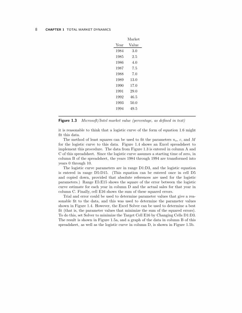
In situations where there is substantial sales data available, standard curve fittingmethods can be used to determine the parameters for the logistic growth curve.As an example, consider the data shown in Figure 1.3 for the market value ofMicrosoft and Intel as a percentage of the total market value for Microsoft, Intel,IBM, and Digital over the period 1984 through 1994 (Modis, 1998, Figure 1-4).The market value data is presumably correlated with product sales, and therefore

8 CHAPTER 1 TOTAL MARKET DYNAMICS

Market

Year Value

1984 3.0

1985 2.5

1986 4.0

1987 7.5

1988 7.0

1989 13.0

1990 17.0

1991 29.0

1992 46.5

1993 50.0

1994 49.5

Figure 1.3 Microsoft/Intel market value (percentage, as defined in text)

it is reasonable to think that a logistic curve of the form of equation 1.6 mightfit this data.

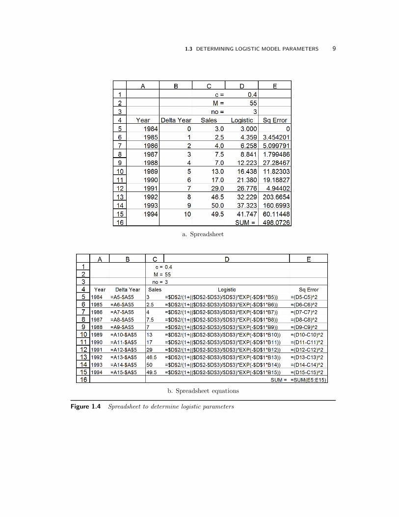
The method of least squares can be used to fit the parameters no, c, and Mfor the logistic curve to this data. Figure 1.4 shows an Excel spreadsheet toimplement this procedure. The data from Figure 1.3 is entered in column A andC of this spreadsheet. Since the logistic curve assumes a starting time of zero, incolumn B of the spreadsheet, the years 1984 through 1994 are transformed intoyears 0 through 10.

The logistic curve parameters are in range D1:D3, and the logistic equationis entered in range D5:D15. (This equation can be entered once in cell D5and copied down, provided that absolute references are used for the logisticparameters.) Range E5:E15 shows the square of the error between the logisticcurve estimate for each year in column D and the actual sales for that year incolumn C. Finally, cell E16 shows the sum of these squared errors.

Trial and error could be used to determine parameter values that give a rea-sonable fit to the data, and this was used to determine the parameter valuesshown in Figure 1.4. However, the Excel Solver can be used to determine a bestfit (that is, the parameter values that minimize the sum of the squared errors).To do this, set Solver to minimize the Target Cell E16 by Changing Cells D1:D3.The result is shown in Figure 1.5a, and a graph of the data in column B of thisspreadsheet, as well as the logistic curve in column D, is shown in Figure 1.5b.

1.3 DETERMINING LOGISTIC MODEL PARAMETERS 9

a. Spreadsheet

b. Spreadsheet equations

Figure 1.4 Spreadsheet to determine logistic parameters

10 CHAPTER 1 TOTAL MARKET DYNAMICS

a. Spreadsheet with best fit logistic curve parameters

b. Plots of data and logistic curve

Figure 1.5 Logistic fit to Figure 1.3 data

1.5 EXERCISES 11

1.4 References

C. J. Farrell, “A Theory of Technological Progress,” Technological Forecastingand Social Change, Vol. 44, pp. 161–178 (1993).

J. C. Fisher and R. H. Pry, “A Simple Substitution Model of TechnologicalChange,” Technological Forecasting and Social Change, Vol. 3, pp. 75–88(1971).

T. Modis, Conquering Uncertainty: Understanding Corporate Cycles and Posi-tioning Your Company to Survive the Changing Environment, McGraw-Hill,New York, 1998.

J. Roughgarden, Primer of Ecological Theory, Prentice Hall, Upper Saddle River,New Jersey, 1998.

1.5 Exercises

1.1 The following table shows the percentage of total revenue for Arthur An-derson generated by consulting activities over the period 1980 through 1995(Modis, 1998, Figure 1-5).

Year Revenue

1980 48.5

1981 50.0

1982 50.5

1983 51.0

1984 52.5

1985 53.5

1986 57.0

1987 60.0

1988 63.5

1989 67.0

1990 68.5

1991 71.0

1992 72.0

1993 71.5

1994 75.5

1995 76.0

A plot of this data shows that it has a logistic curve shape, except thatthe initial value of this curve is not at zero. This can be explained by

12 CHAPTER 1 TOTAL MARKET DYNAMICS

the following hypothesis: Prior to approximately 1980, consulting serviceswere an approximately stable portion of total Arthur Anderson revenue.Then, starting in 1980, consulting services started to be purchased by anew market (for example, computer systems consulting), and the growthof this new market followed a logistic process.

For the remainder of this exercise, assume that the “base revenue” forconsulting prior to 1980 was 45 per cent of total revenue, and work withthe revenue increase above this base revenue amount, rather than with theraw revenue numbers given in the table above.

(i) Follow the procedure demonstrated in Section 1.3 to determine the“best fit” parameters for a logistic curve fit to the revenue increaseover the period 1980 through 1995.

(ii) Plot the actual revenue increase data shown in the table above on thesame graph with the logistic curve fit determined in the precedingquestion.

(ii) Determine the logistic curve estimate for the ultimate percentage ofArthur Anderson total revenue that consulting will attain.

C H A P T E R 2

CompetitiveMarketDynamics

In this chapter, the models developed in the preceeding chapter are extended tosituations where there are competitors who are each attempting to sell a durablegood to the same set of Potential Customers. We assume that the PotentialCustomers only purchase the durable good once, and therefore if a PotentialCustomer purchases from one of the competitors, that Potential Customer islost forever to the other competitors.

We will use the same word-of-mouth modeling approach as in the precedingchapter for each of the competitors. That is, we will assume that PotentialCustomers become Actual Customers for each of the competitors in proportionto the number of Actual Customers for that competitor. We will restrict our-selves to situations with two competitors, although generalizing to more thantwo competitors is straightforward.

2.1 Infinite Potential Customers

First, consider the situation where the number of Potential Customers is in-finitely large compared to the number of Actual Customers. Assume that fora short period of time ∆t each Actual Customer of competitor number i con-verts ci∆t Potential Customers into Actual Customers for competitor number i,where ci is a positive constant that encodes how effective Actual Customers forcompetitor i are at converting Potential Customers.

If at time t there are ni(t) Actual Customers for competitor i, each of whichconverts ci∆t Potential Customers into Actual Customers for competitor i duringthe next ∆t time period, then at time t + ∆t the number of Actual Customersfor competitor i will be ni(t + ∆t) = ni(t) + ni(t)ci∆t.

This leads to the differential equations

dn1(t)

dt= c1n1(t) (2.1)

dn2(t)

dt= c2n2(t) (2.2)

14 CHAPTER 2 COMPETITIVE MARKET DYNAMICS

or the corresponding integral equations

n1(t) = n1o +

∫ t

0

c1n1(τ ) dτ (2.3)

n2(t) = n2o +

∫ t

0

c2n2(τ ) dτ (2.4)

where nio is the number of Actual Customers for competitor i at time t = 0. Sinceequations 2.1 and 2.2 (or equivalently, equations 2.3 and 2.4) are independent ofeach other, then n1(t) and n2(t) will not depend on each other. Hence, from thearguments in the preceding chapter, the solution to these equations are

ni(t) = nioecit, t ≥ 0, i = 1, 2 (2.5)

Thus, in a situation with an infinite number of Potential Customers, the twocompetitors can happily ignore each other and blissfully attract new customers.

2.2 Finite Potential Customers

The situation is different when there are a finite number of Potential CustomersM . We will make an analogous assumption to that in the preceding chapterwith respect to how Potential Customers are converted into Actual Customersfor each competitor. That is, the number of Potential Customers converted byeach Actual Customer of competitor i into additional Actual Customers for com-petitor i in a time interval ∆t when there are M remaining Potential Customersis ci∆t, and the number converted varies linearly with the remaining proportion[M−n1(t)−n2(t)]/M of unconverted Potential Customers. [Both n1(t) and n2(t)appear in the numerator of this expression because both of the competitors aresimultaneously removing customers from the Potential Customer pool.]

With this assumption, the number of Potential Customers converted by eachActual Customer of competitor i into additional Actual Customers of competitori in a time interval ∆t is {[M −n1(t)−n2(t)]/M}× ci∆t, and hence the numberof Potential Customers converted by all ni(t) Actual Customers of competitor iis ni(t) × {[M − n1(t) − n2(t)]/M} × ci∆t.

Thus, using analogous arguments to those presented above for equations 2.1through 2.4, these assumptions lead to the differential equations

dn1(t)

dt= c1 ×

M − n1(t) − n2(t)

M× n1(t) (2.6)

dn2(t)

dt= c2 ×

M − n1(t) − n2(t)

M× n2(t) (2.7)

or the equivalent integral equations

n1(t) = n1o +

∫

t

0

c1 ×M − n1(τ ) − n2(τ )

M× n1(τ ) dτ (2.8)

n2(t) = n2o +

∫ t

0

c2 ×M − n1(τ ) − n2(τ )

M× n2(τ ) dτ (2.9)

2.3 BANDWAGON MARKETS 15

These equations are special cases of the Lotka-Volterra competition equationsthat have been extensively studied in ecology (Roughgarden 1998).

There are not closed form solutions to these equations, but before we turn tonumerical solutions of them, we will generalize equation 2.7 to the following:

dn2(t)

dt=

{

0, t < toc2 ×

M−n1(t)−n2(t)M

× n2(t), t ≥ to(2.10)

That is, we assume that competitor number 2 does not start selling its productuntil time t = to. (Of course, when to = 0, equation 2.10 reduces to equation2.7.)

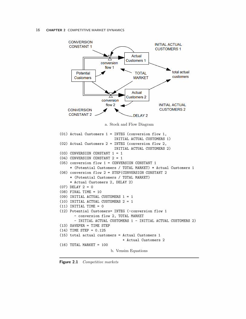
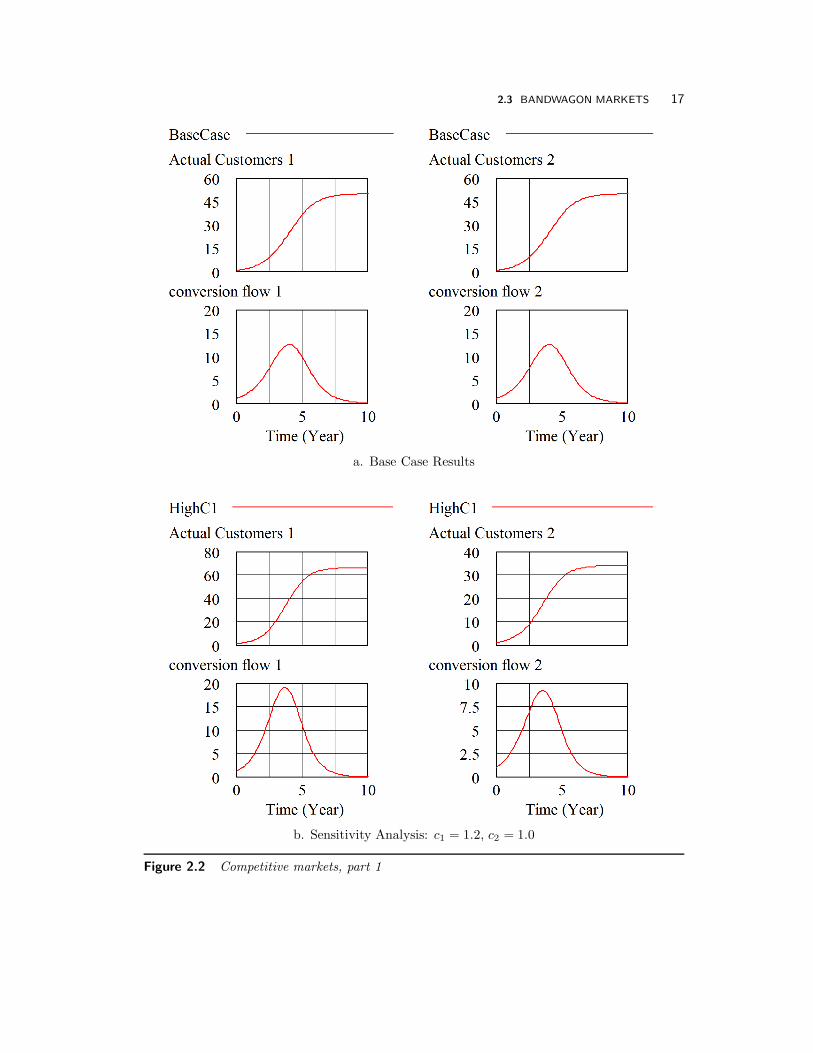
The stock and flow diagram and Vensim equations for this model are shown inFigure 2.1. For the base case analysis, the values of c1 and c2 are set equal, as arethe values of n1o and n2o. The results of running this model are shown in Figure2.2a, and these show the not very surprising result that the two competitors splitthe market equally.

Figure 2.2b shows how things change if the relative attractiveness of competi-tor number 1 increases by twenty per cent to c1 = 1.2. (Note that the verticalscales are different for the two graphs in Figure 2.2b.) Not surprisingly, competi-tor number 1 attracts substantially more customers in this situation. However,the impact of the twenty per cent increase on the final market share is more thantwenty per cent. Competitor number 1 ends up with about sixty-six per centof the market, while competitor number 2 only has about thirty-four per cent.Thus, the twenty per cent advantage in c1 translates into a thirty-two per cent[(66 − 50)/50] improvement in market share, or a 66/34 = 1.94 ratio in marketshare advantage.

Figure 2.3 illustrates how other asymmetries between the two competitorsimpact the market share. In Figure 2.3a, the initial number of Actual Customersn1o for competitor number 1 is increased from the base case of one to two. Asthe figure shows, this has a similar impact on market share to increasing c1 to1.2.

In Figure 2.3b, competitor number 2 is delayed in starting to market a productby 0.75 years (nine months), and this also has a similar impact on market shareto increasing c1 to 1.2.

2.3 Bandwagon Markets

The model of competition in the preceding section assumes that the effective-ness of Actual Customers for each competitor in recruiting Potential Customersremains constant over time in the following sense: The rate at which any par-ticular Actual Customer recruits any particular Potential Customer is c1/M forActual Customers of competitor number 1 and c2/M for Actual Customers ofcompetitor number 2. This remains constant over time and regardless of thenumber of Actual or Potential Customers. (That is, the variation in the flow ofnew Actual Customers results from the fact that the numbers of Potential and

16 CHAPTER 2 COMPETITIVE MARKET DYNAMICS

a. Stock and Flow Diagram

(01) Actual Customers 1 = INTEG (conversion flow 1,

INITIAL ACTUAL CUSTOMERS 1)

(02) Actual Customers 2 = INTEG (conversion flow 2,

INITIAL ACTUAL CUSTOMERS 2)

(03) CONVERSION CONSTANT 1 = 1

(04) CONVERSION CONSTANT 2 = 1

(05) conversion flow 1 = CONVERSION CONSTANT 1

* (Potential Customers / TOTAL MARKET) * Actual Customers 1

(06) conversion flow 2 = STEP(CONVERSION CONSTANT 2

* (Potential Customers / TOTAL MARKET)

* Actual Customers 2, DELAY 2)

(07) DELAY 2 = 0

(08) FINAL TIME = 10

(09) INITIAL ACTUAL CUSTOMERS 1 = 1

(10) INITIAL ACTUAL CUSTOMERS 2 = 1

(11) INITIAL TIME = 0

(12) Potential Customers= INTEG (-conversion flow 1

- conversion flow 2, TOTAL MARKET

- INITIAL ACTUAL CUSTOMERS 1 - INITIAL ACTUAL CUSTOMERS 2)

(13) SAVEPER = TIME STEP

(14) TIME STEP = 0.125

(15) total actual customers = Actual Customers 1

+ Actual Customers 2

(16) TOTAL MARKET = 100

b. Vensim Equations

Figure 2.1 Competitive markets

2.3 BANDWAGON MARKETS 17

a. Base Case Results

b. Sensitivity Analysis: c1 = 1.2, c2 = 1.0

Figure 2.2 Competitive markets, part 1

18 CHAPTER 2 COMPETITIVE MARKET DYNAMICS

a. Sensitivity Analysis: n1o = 2, n2o = 1

b. Sensitivity Analysis: to = 0.75

Figure 2.3 Competitive markets, part 2

2.4 REFERENCES 19

Actual Customers is varying, and not from a variation in the effectiveness of the“word of mouth” for Actual Customers of the two competitors.)

However, it has been pointed out (Arthur 1990) that in some markets theeffectiveness of recruiting appears to change depending on the number of ActualCustomers. There is a so-called “bandwagon effect” where the effectiveness ofthe recruiting increases as the number of Actual Customers for a particularcompetitor increases. This can be explained by saying that Potential Customerswant to “go with a winner,” or are afraid of purchasing a less popular productthat might then be orphaned.

This phenomenon can be represented by replacing equations 2.6 and 2.10 withthe following:

dn1(t)

dt= c1 × f1[n1(t)/M ]×

M − n1(t) − n2(t)

M× n1(t) (2.11)

dn2(t)

dt=

{

0, t < toc2 × f2[n2(t)/M ] × M−n1(t)−n2(t)

M× n2(t), t ≥ to

(2.12)

In these equations, f1[n1(t)/M ] and f2[n2(t)/M ] represent the impact of thebandwagon effect. Of course, if fi[ni(t)/M ] = 1, then equations 2.11 and 2.12reduce to 2.6 and 2.10, respectively.

To investigate the impact of the bandwagon effect, assume that fi varieslinearly with respect to its argument. Specifically,

fi(x) = si × x + (1 − si/2), (2.13)

where si is the slope of a straight line. Note that with this equation form,fi(1/2) = 1 regardless of the value of si.

We might expect that in many cases, s1 = s2, and a Vensim model of equations2.11 and 2.12 for this case is shown in Figure 2.4, with si = 1.5.

The results of simulation runs for this model corresponding to those shown inFigure 2.2 and Figure 2.3 are shown in Figure 2.5 and Figure 2.6. Note that withbandwagon effects, a differential advantage of one competitor translates into agreater market share advantage than in the models of the preceding section. Theresult is more of a “winner take all” situation.

2.4 References

W. B. Arthur, “Positive Feedbacks in the Economy,” Scientific American,Vol. 262, No. 2, pp. 92–99 (February 1990).

J. Roughgarden, Primer of Ecological Theory, Prentice Hall, Upper Saddle River,New Jersey, 1998.

20 CHAPTER 2 COMPETITIVE MARKET DYNAMICS

a. Stock and Flow Diagram

(01) Actual Customers 1 = INTEG (conversion flow 1,INITIAL ACTUAL CUSTOMERS 1)

(02) Actual Customers 2 = INTEG (conversion flow 2,INITIAL ACTUAL CUSTOMERS 2)

(03) CONVERSION CONSTANT 1 = 1(04) CONVERSION CONSTANT 2 = 1(05) conversion flow 1 = CONVERSION CONSTANT 1

* (EFFECTIVENESS SLOPE * (Actual Customers 1/ TOTAL MARKET) + (1 - (EFFECTIVENESS SLOPE / 2)))

* (Potential Customers / TOTAL MARKET) * Actual Customers 1(06) conversion flow 2 = STEP(CONVERSION CONSTANT 2

* (EFFECTIVENESS SLOPE * (Actual Customers 2 / TOTAL MARKET)+ (1 - (EFFECTIVENESS SLOPE / 2))) * (Potential Customers /

TOTAL MARKET) * Actual Customers 2, DELAY 2)(07) DELAY 2 = 0(08) EFFECTIVENESS SLOPE = 1.5(09) FINAL TIME = 20(10) INITIAL ACTUAL CUSTOMERS 1 = 1(11) INITIAL ACTUAL CUSTOMERS 2 = 1(12) INITIAL TIME = 0(13) Potential Customers= INTEG (-conversion flow 1

- conversion flow 2, TOTAL MARKET- INITIAL ACTUAL CUSTOMERS 1 - INITIAL ACTUAL CUSTOMERS 2)

(14) SAVEPER = TIME STEP(15) TIME STEP = 0.125(16) total actual customers = Actual Customers 1

+ Actual Customers 2(17) TOTAL MARKET = 100

b. Vensim Equations

Figure 2.4 Bandwagon effect

2.4 REFERENCES 21

a. Base Case Results

b. Sensitivity Analysis: c1 = 1.2, c2 = 1.0

Figure 2.5 Bandwagon effects, part 1

22 CHAPTER 2 COMPETITIVE MARKET DYNAMICS

a. Sensitivity Analysis: n1o = 2, n2o = 1

b. Sensitivity Analysis: to = 0.75

Figure 2.6 Bandwagon effects, part 2