NREL is a national laboratory of the U.S. Department of Energy, Office of Energy Efficiency & Renewable Energy, operated by the Alliance for Sustainable Energy, LLC.

Contract No. DE-AC36-08GO28308

The New Modularization Framework for the FAST Wind Turbine CAE Tool Preprint J. Jonkman To be presented at the 51st AIAA Aerospace Sciences Meeting, including the New Horizons Forum and Aerospace Exposition Dallas, Texas January 7-10, 2013

Conference Paper NREL/CP-5000-57228 January 2013

NOTICE

The submitted manuscript has been offered by an employee of the Alliance for Sustainable Energy, LLC (Alliance), a contractor of the US Government under Contract No. DE-AC36-08GO28308. Accordingly, the US Government and Alliance retain a nonexclusive royalty-free license to publish or reproduce the published form of this contribution, or allow others to do so, for US Government purposes.

This report was prepared as an account of work sponsored by an agency of the United States government. Neither the United States government nor any agency thereof, nor any of their employees, makes any warranty, express or implied, or assumes any legal liability or responsibility for the accuracy, completeness, or usefulness of any information, apparatus, product, or process disclosed, or represents that its use would not infringe privately owned rights. Reference herein to any specific commercial product, process, or service by trade name, trademark, manufacturer, or otherwise does not necessarily constitute or imply its endorsement, recommendation, or favoring by the United States government or any agency thereof. The views and opinions of authors expressed herein do not necessarily state or reflect those of the United States government or any agency thereof.

Available electronically at http://www.osti.gov/bridge

Available for a processing fee to U.S. Department of Energy and its contractors, in paper, from:

U.S. Department of Energy Office of Scientific and Technical Information P.O. Box 62 Oak Ridge, TN 37831-0062 phone: 865.576.8401 fax: 865.576.5728 email: mailto:reports@adonis.osti.gov

Available for sale to the public, in paper, from:

U.S. Department of Commerce National Technical Information Service 5285 Port Royal Road Springfield, VA 22161 phone: 800.553.6847 fax: 703.605.6900 email: orders@ntis.fedworld.gov online ordering: http://www.ntis.gov/help/ordermethods.aspx

Cover Photos: (left to right) PIX 16416, PIX 17423, PIX 16560, PIX 17613, PIX 17436, PIX 17721

Printed on paper containing at least 50% wastepaper, including 10% post consumer waste.

1

The New Modularization Framework for the FAST Wind Turbine CAE Tool*

Jason M. Jonkman† National Renewable Energy Laboratory (NREL), Golden, Colorado, 80401

NREL recently has put considerable effort into improving the overall modularity of its FAST wind turbine aero-hydro-servo-elastic tool to (1) improve the ability to read, implement, and maintain source code; (2) increase module sharing and shared code development across the wind community; (3) improve numerical performance and robustness; and (4) greatly enhance flexibility and expandability to enable further developments of functionality without the need to recode established modules. The new FAST modularization framework supports module-independent inputs, outputs, states, and parameters; states in continuous-time, discrete-time, and constraint form; loose and tight coupling; independent time and spatial discretizations; time marching, operating-point determination, and linearization; data encapsulation; dynamic allocation; and save/retrieve capability. This paper explains the features of the new FAST modularization framework, as well as the concepts and mathematical background needed to understand and apply it correctly. It is envisioned that the new modularization framework will transform FAST into a powerful, flexible, and robust wind turbine modeling tool with a large number of developers and a range of modeling fidelities across the aerodynamic, hydrodynamic, servo-dynamic, and structural-dynamic components.

Nomenclature A = continuous-state matrix for linearized continuous-state equations AADC = continuous-state matrix for linearized discrete-state equations Ad = discrete-state matrix for linearized discrete-state equations ADAC = discrete-state matrix for linearized continuous-state equations B = input matrix for linearized continuous-state equations BADC = input matrix for linearized discrete-state equations C = continuous-state matrix for linearized output equations CDAC = discrete-state matrix for linearized output equations D = input-transmission matrix for linearized output equations

G = the matrix formed by 1U U Z Z

u z z u

−∂ ∂ ∂ ∂ − ∂ ∂ ∂ ∂

H( ) = Heaviside-step (unit-step) function n = discrete-step counter N = total number of modules coupled together p(t) = parameters t = time u(t) = inputs U( ) = input-output transformation functions

*The submitted manuscript has been offered by an employee of the Alliance for Sustainable Energy, LLC (Alliance), a contractor of the US Government under Contract No. DE-AC36-08GO28308. Accordingly, the U.S. Government and Alliance retain a nonexclusive royalty-free license to publish or reproduce the published form of this contribution, or allow others to do so, for US Government purposes. †Senior Engineer, National Wind Technology Center (NWTC), 15013 Denver West Parkway, AIAA Professional Member.

2

x(t) = continuous states ( )x t = first time derivative of the continuous states

X( ) = continuous-state functions xd[n] = discrete states Xd( ) = discrete-state functions y(t) = outputs Y( ) = output functions z(t) = constraint (algebraic) states Z( ) = constraint-state (algebraic) functions Δt = discrete time step (increment)

I. Introduction HE wind industry relies extensively on computer-aided-engineering (CAE) tools for wind turbine performance, loads, and stability analyses. Limitations—and consequent inaccuracies—in the tools slow the advancement of

wind power. Accurate tools are required for the wind industry to develop more innovative, optimized, reliable, and cost-effective wind technology. Overcoming current modeling limitations increases in importance as turbines scale up to larger sizes, incorporate novel architectures and load-control technologies, and are installed on offshore support platforms.

Over the past two decades, the U.S. Department of Energy (DOE) has sponsored NREL’s development of CAE tools for wind turbine analysis. The tools are developed as free, publicly available, open-source, professional-grade products as a resource for the wind industry. The tools are used by thousands of wind turbine designers, manufacturers, consultants, certifiers, researchers, educators, and students throughout the world. The open-source approach facilitates the tools’ credibility and adaptability by the wind industry. The tools are modular, well documented, and supported by NREL through workshops and an on-line forum. They have been verified through model-to-model comparisons and validated with test measurements.

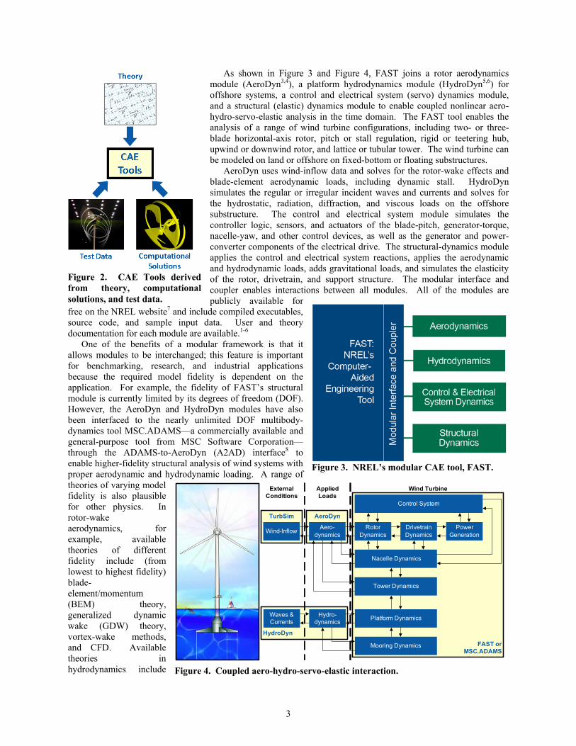
Analyzing wind-energy structures requires CAE tools that model the important physical phenomena (illustrated in Figure 1) and system couplings, including the environmental excitation (wind, waves, and current) and full-system dynamic response (rotor, drivetrain, nacelle, support structure, and controller).

However, industry design work demands that CAE tools run on typical computers because the certification-driven design process is iterative and must consider a vast set of environmental conditions and operational scenarios. Computationally intensive solutions are generally unsuitable for these applications because the long run times make it impossible to consider all of the required cases. So, CAE tools cannot solely be massively discretized high-performance computing (HPC) solutions of the fundamental laws of physics (e.g., computational fluid dynamics (CFD) solutions of the Navier-Stokes equations). Instead, NREL’s core CAE tool, FAST,1,2 is based on advanced engineering models—derived from fundamental laws, but with appropriate simplifications and assumptions, and supplemented where applicable with computational solutions and test data, as illustrated in Figure 2.

T

Figure 1. Physical phenomena affecting a floating wind turbine system.

3

As shown in Figure 3 and Figure 4, FAST joins a rotor aerodynamics module (AeroDyn3,4), a platform hydrodynamics module (HydroDyn5,6) for offshore systems, a control and electrical system (servo) dynamics module, and a structural (elastic) dynamics module to enable coupled nonlinear aero-hydro-servo-elastic analysis in the time domain. The FAST tool enables the analysis of a range of wind turbine configurations, including two- or three-blade horizontal-axis rotor, pitch or stall regulation, rigid or teetering hub, upwind or downwind rotor, and lattice or tubular tower. The wind turbine can be modeled on land or offshore on fixed-bottom or floating substructures.

AeroDyn uses wind-inflow data and solves for the rotor-wake effects and blade-element aerodynamic loads, including dynamic stall. HydroDyn simulates the regular or irregular incident waves and currents and solves for the hydrostatic, radiation, diffraction, and viscous loads on the offshore substructure. The control and electrical system module simulates the controller logic, sensors, and actuators of the blade-pitch, generator-torque, nacelle-yaw, and other control devices, as well as the generator and power-converter components of the electrical drive. The structural-dynamics module applies the control and electrical system reactions, applies the aerodynamic and hydrodynamic loads, adds gravitational loads, and simulates the elasticity of the rotor, drivetrain, and support structure. The modular interface and coupler enables interactions between all modules. All of the modules are publicly available for

free on the NREL website7 and include compiled executables, source code, and sample input data. User and theory documentation for each module are available.1-6

One of the benefits of a modular framework is that it allows modules to be interchanged; this feature is important for benchmarking, research, and industrial applications because the required model fidelity is dependent on the application. For example, the fidelity of FAST’s structural module is currently limited by its degrees of freedom (DOF). However, the AeroDyn and HydroDyn modules have also been interfaced to the nearly unlimited DOF multibody-dynamics tool MSC.ADAMS—a commercially available and general-purpose tool from MSC Software Corporation—through the ADAMS-to-AeroDyn (A2AD) interface8 to enable higher-fidelity structural analysis of wind systems with proper aerodynamic and hydrodynamic loading. A range of theories of varying model fidelity is also plausible for other physics. In rotor-wake aerodynamics, for example, available theories of different fidelity include (from lowest to highest fidelity) blade-element/momentum (BEM) theory, generalized dynamic wake (GDW) theory, vortex-wake methods, and CFD. Available theories in hydrodynamics include

Figure 3. NREL’s modular CAE tool, FAST.

FAST orMSC.ADAMS

HydroDyn

AeroDyn

External Conditions

Applied Loads

Wind Turbine

TurbSim

Hydro-dynamics

Aero-dynamics

Waves & Currents

Wind-Inflow Power Generation

Rotor Dynamics

Platform Dynamics

Mooring Dynamics

Drivetrain Dynamics

Control System

Nacelle Dynamics

Tower Dynamics

Figure 4. Coupled aero-hydro-servo-elastic interaction.

Figure 2. CAE Tools derived from theory, computational solutions, and test data.

4

Morison’s equation with linear waves; Morison’s equation with higher-order waves; potential-flow theory with linear radiation, diffraction, and hydrostatics; second-order potential-flow theory; and CFD. Many of these theories have not been implemented within FAST, but would be of great value. There are also many CAE tools where these individual theories have been implemented (e.g., the Aerodynamic Wind turbine Simulation Module (AWSM)9 from the Energy research Centre of the Netherlands (ECN) for the vortex-wake method), but most have not yet been interfaced with FAST. The concept of interchanging modules is illustrated in Figure 5, although in practice all modules are interfaced through a common driver program (i.e., modular interface and coupler or “glue code”) as illustrated in Figure 3.

While the FAST CAE tool has always been modular, NREL recently has put considerable effort into improving its overall modularity to accomplish the following benefits: (1) improved ability to read, implement, and maintain source code; (2) increased module sharing and shared code development across the wind community; (3) improved numerical performance and robustness; and (4) greatly enhanced flexiblity and expandability to enable further developments of functionality without the need to recode established modules. It is envisioned that the new modularization framework will transform FAST into a powerful, flexible, and robust wind turbine CAE tool with a large number of developers and a range of modeling fidelities across the aerodynamic, hydrodynamic, servo-dynamic, and structural-dynamic components.

This paper explains the features of the new FAST modularization framework, as well as the concepts and mathematical background needed to understand and apply it correctly. Specific problems with earlier versions of FAST that the new modularization framework addresses are summarized in Table 1 and are discussed where

appropriate in this paper. While not covered in this paper, a programmer’s handbook10 explaining the code development requirements and best practices has been written to support shared code development across the wind community. The handbook includes a Fortran-based‡ source-code template for developing modules within the framework, including the necessary data structures and interface procedures. Please note that the current FAST source code at the time of publication (v7.02.00d-bjj) does not yet conform to this framework; effort is being made to convert to this new framework.

‡Mixed-language programming (e.g., with C-based source code) is possible through appropriate adaptations.

Table 1. Summary of problems and solutions addressed by the new FAST modularization framework.

Problem Solution

• Limited range of modeling fidelity• Framework allowing modules to be exchanged• Development of new modules of higher fidelity

• Solution driven by structural solver • Separate module interface and coupler

• Inability to isolate a given model• Modules that can be called by separate driver programs or interfaced together to form a coupled solution

• Dependent spatial discretizations and time steps across modules

• Library of spatial elements and mesh-to-mesh mapping• Data transfer with interpolation/extrapolation in time

• Inability to linearize all system equations

• Tight coupling with options for operating-point determination and linearization

• Focus on single turbine• Dynamic allocation of modules for wind-plant simulation

• “Spaghetti code” due to unclear data transfer and global data

• Modularization with data encapsulation

• Limited number of developers due to code size & complexity

• Modularization of code into separate components• Programmer’s handbook explaining code development requirements and best practices

• Potentially poor numerical accuracy and stability

• Multiple coupling schemes and integration/solver options

Figure 5. Conceptualization of module interchange.

5

II. Features of the New Modularization Framework At its core, the new FAST modularization framework is a means by which various mathematical systems

(modeling the important physical phenomena as illustrated in Figure 1) are implemented in distinct modules and interconnected to solve for the global, coupled, dynamic response of a wind turbine system. The new FAST modularization framework supports module-independent inputs, outputs, states, and parameters; states in continuous-time, discrete-time, and constraint form; loose and tight coupling; independent time and spatial discretizations; time marching, operating-point determination, and linearization; data encapsulation; dynamic allocation; and save/retrieve capability. While not covered in this paper, modularization also establishes a basis for mixed-language programming, multicore processing, co-simulation across a network, hiding the details of individual model components to protect intellectual property (IP), and developing hardware-in-the-loop (HIL) simulation.

A. Inputs, Outputs, States, and Parameters Mathematical models of dynamic systems can be developed in terms of inputs, outputs, states, and parameters.

Inputs (identified in this paper by u) are a set of values supplied to a system (i.e., module) and that, together with the states, are needed to calculate future states and/or the system’s output. Outputs (y) are a set of values calculated by and returned from a system and dependent on the system’s states, inputs, and/or parameters through output equations (with functions Y). States are a set of internal values of a system influenced by inputs and/or time and used to calculate future state values and/or the system’s output. There are three types of states. Continuous states (x) are states that are differentiable in time and characterized by continuous-time differential equations (with functions X). Discrete states (with functions xd) are states that only have a value at discrete steps in time and are characterized by discrete-time difference (recurrence) equations (with functions Xd). Constraint states (z) are states that are not differentiated or discrete (i.e., constraint states are algebraic variables) and are characterized by algebraic constraint equations (i.e., equations without time derivatives) (with functions Z). Parameters (p) are a set of internal system values, independent of the states and inputs, that can be fully defined at initialization (possibly with time-dependence that can be fully prescribed at initialization) and characterize a system’s state equations (differential, difference, and/or constraint) and output equations.

As examples in the wind turbine application, structural displacements and velocities are typically represented as continuous states (structural accelerations are not states themselves, but are time derivatives of the velocity states), control-system logic and dynamic-stall formulations are often implemented with discrete states, and structural joints impose constraint states; BEM wake models and other quasi-static or quasi-steady formulations also involve constraint states. For a rotor-aerodynamics module, examples of inputs and outputs include blade-element motion (position, orientation, and translational and rotational velocity) and blade-element loads (forces and moments), respectively. Examples of parameters include structural definitions such as blade and tower length, mass, and stiffness and time-only-dependent environmental conditions such as wind inflow and incident waves not influenced by the structural response. These examples, along with a few others, are summarized in Table 2. Table 2. Examples of inputs, outputs, states, and parameters in the wind turbine application.

Variable Aerodynamics Hydrodynamics Controller Structural Dynamics

• Inputs• Turbine displacements• Turbine velocities

• Substructure displacements• Substructure velocities

• Structural accelerations• Reaction loads

• Aerodynamic loads• Hydrodynamic loads• Controller commands

• Outputs • Aerodynamic loads • Hydrodynamic loads • Controller commands

• Displacements• Velocities• Accelerations• Reaction Loads

• Continuous states • Induction in GDW• State-space-based radiation "memory"

• Analog control signals• Displacements• Velocities

• Discrete states• Beddoes-Leishman dynamic-stall states

• Numerical-convolution- based radiation "memory"

• Digital control signals

• Constraint states • Induction in BEM• Constraint loads at joints• Quasi-static mooring system

• Parameters• Turbine geometry• Static airfoil data• Undisturbed wind inflow

• Substructure geometry• Hydrodynamic coefficients• Undisturbed incident waves

• Controller gains• Controller limits

• Geometry• Mass/inertia• Stiffness coefficients• Damping coefficients

6

The developer can choose a module’s specific inputs, outputs, states, and parameters in the new FAST modularization framework. When choosing inputs for a module as part of the module development process, the only restriction is that a module’s inputs must be algebraically derivable from the available outputs of the modules coupled together (including, perhaps, from the module under development—a recursive formulation)—see Section II.D.

B. Loose and Tight Coupling Before its modularization was improved, FAST applied a loosely coupled time-integration scheme, where data

(inputs and outputs) are exchanged between the modules at each coupling step, but where each module tracks its own states and integrates its own equations with its own solver. Figure 6 illustrates the difference between loose-

and tight-coupling schemes. In a tightly coupled time-integration scheme, each module sets up its own equations, but the states are tracked and integrated by a solver common to all of the modules. The new FAST modularization allows for both loose and tight coupling.

Loose coupling is convenient for introducing legacy code and can be quite computationally efficient because the choice of solver and time steps can be fit-for-purpose to the module. But loose coupling can lead to numerical errors (e.g., drift) or numerical stability problems in the coupled solution in some cases.11,§ These numerical problems can sometimes

be resolved through predictor-corrector-based loose coupling schemes.12 In the new FAST modularization framework, a given loosely coupled module must have a fixed coupling step, and the continuous-time and discrete-time states within a given module must share this time step.

Tight coupling has numerical advantages over loose coupling if the common solver is appropriately suited for the problem; however, the modules have to be developed in a form amenable to tight coupling, which is less common among legacy tools and profoundly impacts how new modules must be developed. Computational performance can be lost in tight coupling because the same (perhaps variable) time step must be applied to all continuous-time states of all interconnected modules. In the new FAST modularization framework, separate modules can have different discrete-time steps, but all of the discrete-time states within a given module must share the same discrete time step. In addition, in the new FAST modularization framework, tight coupling also permits operating-point determination and linearization—see Section II.F.

An initial assessment of the numerical stability, numerical accuracy, and computational performance of various coupling schemes is provided in a companion paper.12

The loose or tight coupling of individual modules is achieved through the modular interface and coupler described in Section II.G. Because of the modularization, it is also possible to isolate the dynamics of an individual module in an uncoupled way. A module in the new FAST modularization framework does not run by itself, but it is called by a separate driver program. The uncoupled solution of a module intended for loose and tight coupling is illustrated in Figure 7.

C. Module Form The mathematical formulation of a module permitted within the new FAST modularization framework is very

general, making the overall framework extremely powerful and flexible enough to be considered for almost any system. A general (need-not-be-linear) state-space formulation is considered with any combination of continuous- §While there is no evidence that numerical errors have influenced the solution of FAST calculations to date, such problems will arise in some cases if the coupling scheme is not addressed appropriately. Numerical problems are known to exist for other CAE tools when coupling modules with (1) effective inertias that are of similar magnitude, (2) characteristic frequencies or length scales that vary greatly, or (3) solver types that are too dissimilar. For example, in some CAE tools for offshore floating wind turbines, the loose coupling of a dynamic mooring system module with an aero-hydro-servo-elastic tool has been known to introduce numerical problems.11

Mod

ular

Inte

rface

and

Coup

ler

Mod

ular

Inte

rfac

ean

d Co

uple

r

( )

( )

( )

Module 1

Module 2

Module N

∫

∫

∫

( )

( )

( )

Module 1

Module 2

Module N

∫

Figure 6. Loose- (left) and tight- (right) coupling schemes.

D r iv e rP r o g r a m

M o d u le∫

D r iv e rP r o g r a m M o d u le∫

Figure 7. Uncoupled solution of a module intended for loose (left) and tight (right) coupling.

7

time-state, discrete-time-state, constraint-state, and output equations. No assumption is made about the theory from which the state-space formulation was derived. A system described by partial differential equations (PDEs) in space and time can be written in a general state-space formulation once the spatial dimensions have been discretized. If no states are present, the system is often referred to as a “feed-forward only system.” If both continuous and discrete states are present, the system is often referred to as a “sampled system” or “hybrid system.” If there are no constraint states, the continuous-time state equations form ordinary differential equations (ODEs), which have well-understood numerical solutions. With constraint states, the system is characterized by differential algebraic equations (DAEs)—that is, differential equations combined with algebraic constraint equations—which are much harder to solve.13

The tight-coupling feature of the new FAST modularization framework permits systems of the form of a hybrid semi-explicit DAE of index 1. This form—as described in more detail below—has only the following limitations: (1) the continuous-time state derivatives and discrete-time state updates must be written as an explicit function of the states, inputs, and parameters and (2) the constraints must be of index 1. These are the same limitations imposed within even the most advanced solvers available in the popular MATLAB/Simulink commercial computing package.14 The most general form allowed by the framework in tight coupling is represented mathematically as

( )dx X x,x ,z,u,t= , · (1a)

[ ] [ ]( )d d dt n t t n t t n t t n t

x n 1 X x ,x n ,z ,u ,t∆ ∆ ∆ ∆= = = =

+ = , · (1b)

( )d0 Z x,x ,z,u,t= with Z 0z

∂≠

∂, and (1c)

( )dy Y x,x ,z,u,t= . · (1d)

The continuous states, x, are defined by the explicit first-order ODEs of Eq. (1a) with the continuous-state functions, X, on the right-hand side (RHS). The continuous states are time dependent, so, x(t) is implied by x where t is time and x is the first time derivative of x. The continuous-state equations are written in first-order form without loss of generality.** The continuous-state functions—as well as the other functions of Eq. (1)—can depend on the continuous states, x, discrete states, xd, constraint states, z, inputs, u, and time, t (and, of course, are characterized by the parameters, p, not shown). Just as x(t) is implied by x, the time-dependency of xd, z, u, and p is also implied. (The direct time dependency of the continuous-state functions—as well as the other functions of Eq. (1)—results from the parameters having direct continuous-time-dependence, p(t), fully prescribed at initialization.) While t is a scalar, it should be understood that x, xd, z, u, and p may be one-dimensional arrays (vectors) of variables, each of different size. X is a vector of the same size as x so that the number of equations matches the number of states.

The discrete states, xd, are defined by the explicit difference (recurrence) equations of Eq. (1b) from step n to n 1+ with the discrete-state functions, Xd, on the RHS. In this paper, square brackets [] in functions denote discrete

**Second-order (or higher) form can easily be reduced to first-order form. For example, if q and q are continuous

states of the second-order system described by ( )dq Q q,q,x ,z,u,t= where q is the second time derivative of q

and Q are the second-order continuous-state equations, first-order form can be realized by using q

xq

=

, with

qx

q

=

and ( )d

qX

Q q,q,x ,z,u,t =

.

In the existing structural module of FAST, the equations of motion take on the generalized form of Newton’s second law, ( ) ( )M q,u,t q F q,q,u,t= , where M is the generalized mass matrix and F is the generalized force vector (no discrete or constraint states are included, but M depends on the displacements and control inputs in general); in this case, ( ) ( ) ( )1Q q,q,u,t M q,u,t F q,q,u,t−= .

8

time whereas round brackets () in functions denote continuous time; the brackets are dropped when implied. The discrete state and discrete-state functions are evaluated only at discrete steps in time based on the fixed discrete time step (interval), Δt, which is greater than zero and the same for all discrete states of a given module. While n and Δt are scalars, Xd is a vector of the same size as xd so that the number of equations matches the number of states. Because the discrete-state functions can depend on continuous-time variables, an analog-to-digital conversion (ADC) is required whereby the continuous-time variables are sampled (evaluated) at the discrete time step, as represented by

t n t∆= in Eq. (1b). Likewise, the zero-order hold (ZOH) method of digital-to-analog conversion

(DAC) is used when continuous-time functions depend on discrete states. Mathematically,

( ) [ ] ( ) ( )( )( )d d

nx t x n H t n t H t n 1 t∆ ∆

∞

=−∞

= − − − +∑ is used in place of xd[n] in all continuous-time

functions, where xd(t) are the discrete states expressed in continuous time and are piecewise constant and H is the Heaviside-step (unit-step) function; although the summation does not have to be implemented in practice, effectively, if xd exists, xd[n] is applied over ( )n t t n 1 t∆ ∆<= < + in all continuous-time functions. Even if discrete states are present in a module, the constraint states, z, inputs, u, outputs, y, and parameters, p, are always expressed in continuous time. (Because they are characterized by continuous-time parameters, p, the discrete-state functions, Xd, are expressed in continuous time even though they are evaluated at discrete time steps.)

The constraint (algebraic) states, z, are defined implicitly in continuous-time form by Eq. (1c) with the constraint-state (algebraic) functions, Z, on the RHS. Z is a vector of the same size as z so that the number of equations matches the number of states. Equation (1c) can be understood in the following context: given the continuous states, x, discrete states, xd, inputs, u, and time, t (and, of course, the parameters, p, not shown), Z can be used to solve for constraint states, z, at time t for use in the other functions of Eq. (1). In tight coupling, the constraints must be of index 1, which means that the constraint-state function must be invertible such that the constraint states could be written as an explicit function of the other states, inputs, and parameters, guaranteeing the local (but not global) existence and uniqueness of a solution. Although the inverse of Z with respect to z does not have to be formulated in practice, it must exist and be bounded in a neighborhood around a solution.

Mathematically, this requires that Z 0z

∂≠

∂, where is used to represent the determinant of the Jacobian matrix

Zz

∂∂

. The requirement Z 0z

∂≠

∂ also means that the matrix inverse of the Jacobian,

1Zz

−∂ ∂

, exists and is

bounded in a neighborhood around a solution, which will be used later. For a system whose DOF result in a naturally higher constraint index (e.g., constraints imposed through Lagrange multipliers in multi-body dynamics often result in index-3 constraints), an index reduction technique must be applied to reduce the index to 1 before the system can be implemented within a tightly coupled module in the new FAST modularization framework. In some systems, it is possible that alternate DOF will naturally result in a lower constraint index.

The outputs, y, are defined explicitly in continuous time by Eq. (1d) with the output functions, Y, on the RHS. Variables y and Y may be one-dimensional arrays (vectors), but of the same size so that the number of equations matches the number of states; the time-dependency of y is also implied. The output equations permit direct feedthrough of input. The output functions need not depend explicitly on the first time derivative of the continuous states, x , because x itself depends on the same variables Y does.

Unlike in tight coupling, a loosely coupled module in the new FAST modularization framework is not limited to a semi-explicit DAE of index 1. An even more general state-space formulation is available in loose coupling (e.g., an index-3 constraint is allowed), but the numerical solution (including time integration) of the loosely coupled equations is implemented by the module developer within the module and the overall solvability, numerical stability, and convergence of the coupled solution is not guaranteed (these can be verified in tight coupling—see Section II.D).

The semi-explicit DAE of index 1 formulation available in Eq. (1) for tight coupling is a subset of the more general formulation available in loose coupling. As such, it is possible (likely desirable) in the FAST modularization framework to develop a given module for both loose and tight coupling when the system is expressible in the semi-explicit DAE of index 1 formulation of Eq. (1).

9

D. Input-Output Transformations and Coupled Solution The module interface and coupler described in Section II.G interconnects all of the individual modules together

and drives the overall coupled solution forward. One key role of the module interface and coupler is to derive the inputs to the individual modules from the available outputs of the modules coupled together.

Given N total number of modules coupled together, the inputs, u, from each individual module can be combined into a single one-dimensional array (vector) across all coupled modules; likewise for the outputs, y,

( )

( )

( )

1

2

N

u

uu

u

=

and

( )

( )

( )

1

2

N

y

yy

y

=

. (2)

In Eq. (2), superscript (i) is used to identify the ith module and u without a superscript denotes the combined vector of inputs across all coupled modules; the same convention is used for the outputs, y. In this paper, it should be clear from the context whether a variable refers to an individual module or the specific variable combined from all modules into a single vector. Also in this paper, curly brackets {} in arrays denote one-dimensional vectors whereas square brackets [] in arrays denote two-dimensional matrices; the brackets are dropped when implied.

The input-output transformation equations used by the new FAST modularization framework in both loose and tight coupling are represented mathematically in their most general form as ( u is defined following Eq. (4) below)

( )0 U u, y,t= with U 0u

∂≠

∂ . (3)

The input-output transformation equations of Eq. (3) are algebraic (that is, without derivatives) and expressed implicitly in continuous time with the input-output transformation functions, U, on the RHS. U is a vector of the same size as u so that the number of equations matches the number of inputs across all modules. If two or more of the modules coupled together share some of the same exact inputs, the size of u and U can be reduced by that same number. Equation (3) can be understood in the following context: given the outputs across all coupled modules, y, and time, t, U can be used to solve for the inputs across all coupled modules, u, at time t. Of course, if modules have direct feedthrough of input to output, the solve can present a problem, as discussed below. The input-output transformation functions must be defined specifically for each collection of modules coupled together. Because no assumption is made about the theory from which each module was derived, it is possible to mix methodologies if the inputs and outputs are compatible. Equation (3) implies that the input of any module is permitted to depend on any module’s output, including, perhaps, a module’s own output—a recursive formulation. To clarify this point, it is useful to identify the input-output transformation equations for each individual module as shown in Eq. (4) below. (Equation (4) is equivalent to Eq. (3), but with input-output transformation for each module identified.) It should be clear by Eq. (4) that while there are separate input-output transformation equations for each module, each transformation can depend on the inputs and outputs across all modules, and so cannot be solved independently from the other modules’ input-output transformations in general. The input-output transformation functions may also depend on time-dependent parameters, implied by the dependency on time, t, in Eqs. (3) and (4). While the general form of the input-output transformation equations expressed in Eqs. (3) and (4) is powerful, it is fairly common for the transformation to be quite trivial.†† ††For example, modules are often developed so that the input of one module equals the output of another, as implied by Table 2. For the case of a two module system each with its input equaling the output of the other, the input-

output transformation equations are ( ) ( )( ) ( )

( ) ( )

( ) ( )

1 1 2

2 2 1

U u, y,t0 u y0 U u, y,t u y

− = = −

with I 0U 1 00 Iu ∂

= = ≠ ∂ and

0 IUI 0y

− ∂= −∂

, where I is the identify matrix.

10

( ) ( )( ) ( )

( ) ( )

1

2

N

U u, y,t00 U u, y,t

0 U u, y,t

=

with

U 0u

∂≠

∂ (4)

Similar to the restriction on constraint index in tight coupling, the input-output transformation functions must be invertible such that the inputs could be written as an explicit function of the outputs, guaranteeing the local (but not global) existence and uniqueness of a solution. This restriction on the input-output transformation functions exists for both loose and tight coupling in the FAST modularization framework. Although the function inverse does not have to be formulated in practice, it must exist and be bounded in a neighborhood around a solution.

Mathematically, this requires that U 0u

∂≠

∂ , where u is a dummy variable representing u that is needed to clarify

that the partial derivative of U is with respect to the u explicitly identified in Eq. (3), or ( )0 U u, y,t= . That is, the partial derivative of U in Eq. (3) does not involve the chain rule with the u that is included in the calculation of y by Eq. (1d). Making use of the chain rule, however, reveals that

U U U Yu u y u

∂ ∂ ∂ ∂= +

∂ ∂ ∂ ∂ and

U U Yz y z

∂ ∂ ∂=

∂ ∂ ∂, (5)

which are used below. Because inputs are derived from outputs and the new FAST

modularization framework permits the output of individual modules to depend directly on their input (i.e., direct feedthrough of input to output), the input-output transformations themselves form algebraic constraint equations. This condition is equivalent to what is referred to as “algebraic loops” in MATLAB/Simulink. In some cases, it is possible that there is no global solution, no local solution, or no solution at all.

In a tightly coupled system, the existence of a solution can be checked, but this is not possible in a loosely coupled system because of the possibility of the more general state-space formulation available with loose coupling. To clarify this point, again consider N total number of modules coupled together, as illustrated in Figure 8, which follows the organization of Figure 6 (without integration shown), but which uses the nomenclature for the state, output, and input functions and inputs and outputs. Just as the inputs and outputs from each individual module were combined across all modules in Eq. (2), the states, state functions, and output functions can be combined into vectors across all modules as well

( )

( )

( )

1

2

N

x

xx

x

=

,

( )

( )

( )

d 1

d 2d

d N

x

xx

x

=

,

( )

( )

( )

1

2

N

z

zz

z

=

, (6a)

( )

( )

( ) ( ) ( ) ( )

( )

( )

( ) ( ) ( ) ( )

( )

( )

( ) ( ) ( ) ( )

1

1 d 1 1 1

1

2

2 d 2 2 2

2

N

N d N N N

N

uX ,X ,Z ,Y

y

uX ,X ,Z ,Y

Uy

uX ,X ,Z ,Y

yy

Figure 8. Coupling of N modules.

11

( )

( )

( )

1

2

N

X

XX

X

=

,

( )

( )

( )

d 1

d 2d

d N

X

XX

X

=

,

( )

( )

( )

1

2

N

Z

ZZ

Z

=

, and

( )

( )

( )

1

2

N

Y

YY

Y

=

. (6b)

Substituting the last of Eq. (6b) and Eq. (1d) into Eq. (3), results in ( )( )d0 U u,Y x,x ,z,u,t ,t= , meaning

that—like the other functions of Eq. (1)—the input-output transformation functions, U, could be written as functions of the continuous states, x, discrete states, xd, constraint states, z, inputs, u, combined across all modules and time, t—that is, ( )d0 U x,x ,z,u,t= . Taking this form of U with Eqs. (2) and (6) together with Eq. (1) and grouping Z

and U reveals that in tight coupling, the coupled solution of all modules forms a global hybrid semi-explicit DAE

( )dx X x,x ,z,u,t= , · (7a)

[ ] [ ]( )d d dt n t t n t t n t t n t

x n 1 X x ,x n ,z ,u ,t∆ ∆ ∆ ∆= = = =

+ = ,· · (7b)

( )( )

d

d

Z x,x ,z,u,t00 U x,x ,z,u,t

=

with

Z Zz u 0U Uz u

∂ ∂ ∂ ∂ ≠ ∂ ∂ ∂ ∂

, and (7c)

( )dy Y x,x ,z,u,t= . · (7d)

Although they appear nearly identical, Eq. (7) should not be confused with Eq. (1). Equation (7) applies to the coupled solution of all modules in tight coupling whereas Eq. (1) applies only to an individual module in tight coupling. Importantly, even if none of the individual modules themselves have internal constraint states (meaning that z and Z are absent from Eqs. (1) and (7)), the coupled solution of all modules still forms a DAE in tight coupling. The inputs across all modules, u, act as additional constraint states defined by the constraint-state (algebraic) equations (which are actually the input-output transformation equations) in Eq. (7c) with the input-output transformation functions, U, on the RHS. Effectively, the coupling illustrated in Figure 8 has been reduced in tight coupling to the system illustrated in Figure 9. Please note that if the discrete time step (interval), Δt, differs between individual modules, separate discrete-state and discrete-state-function groupings are needed, even though they have been shown grouped together in Eq. (7).

To ensure that the global semi-explicit DAE of the coupled solution of all modules in tight coupling has an index of 1, the condition identified by the determinant in Eq. (7c) is needed in addition to the conditions required of the determinants in Eqs. (1c) and (3). Through the properties of determinants of block matrices, it can be shown that

1

Z ZZ U U Z Zz u

U U z u z z uz u

−∂ ∂

∂ ∂ ∂ ∂ ∂ ∂ ∂ = − ∂ ∂ ∂ ∂ ∂ ∂ ∂ ∂ ∂

, (8)

which is nonzero by Eq. (7c). The first determinant on the right of Eq. (8) is nonzero by Eq. (1c) (expanded across all coupled modules), which means that the second determinant on the right of Eq. (8) must also be nonzero. The

d ZX ,X , ,Y

U

y

Figure 9. Effective tightly coupled system.

12

matrix in the second determinant on the right of Eq. (8) will be identified with symbol G from now on. Inserting Eq. (5) into G, it can thus be shown that the condition identified by the determinant in Eq. (7c) is equivalent to

( )

( )

( )

( )

( )

( )

( )

( )

( )

( )

( )

( )

( )

( )

( )

( )

( )

( )

( )

( )

( )

( )

( )

( )

11 1 1 1

1 1 1 1

12 2 2 2

2 2 2 2

1N N N N

N N N N

Y Y Z Z 0 0u z z u

Y Y Z Z0 0U UG u z z uu y

Y Y Z Z0 0u z z u

−

−

−

∂ ∂ ∂ ∂ − ∂ ∂ ∂ ∂ ∂ ∂ ∂ ∂ −∂ ∂ = + ∂ ∂ ∂ ∂ ∂ ∂

∂ ∂ ∂ ∂ − ∂ ∂ ∂ ∂

with G 0≠ , (9)

which means that the matrix inverse 1G− exists as will be used later.

The Jacobian matrices Uu

∂∂

and Uy

∂∂

from Eq. (9) are written out in terms of their relationships between

individual modules in Eq. (10) below. In general, these Jacobian matrices could be fully populated, but in practice they are likely quite sparse.

( )

( )

( )

( )

( )

( )

( )

( )

( )

( )

( )

( )

( )

( )

( )

( )

( )

( )

1 1 1

1 2 N

2 2 2

1 2 N

N N N

1 2 N

U U Uu u uU U UUu u uu

U U Uu u u

∂ ∂ ∂ ∂ ∂ ∂

∂ ∂ ∂∂ = ∂ ∂ ∂ ∂

∂ ∂ ∂ ∂ ∂ ∂

and

( )

( )

( )

( )

( )

( )

( )

( )

( )

( )

( )

( )

( )

( )

( )

( )

( )

( )

1 1 1

1 2 N

2 2 2

1 2 N

N N N

1 2 N

U U Uy y y

U U UU

y y yy

U U Uy y y

∂ ∂ ∂ ∂ ∂ ∂

∂ ∂ ∂ ∂= ∂ ∂ ∂

∂ ∂ ∂ ∂ ∂ ∂ ∂

(10)

The condition identified by Eq. (9) determines the existence of a solution in tight coupling, and can be checked

by the module interface and coupler, provided that the Jacobian matrices Yu

∂∂

, Yz

∂∂

, Zz

∂∂

, and Zu∂∂

are known for

each individual module and Uu

∂∂

and Uy

∂∂

are known. The important role that direct feedthrough of input to

output plays in determining whether a solution exists should be clear by Eq. (9).‡‡ Of course, it is best to check the

‡‡In the two module example of footnote ††,

( )

( )

( )

( )

( )

( )

( )

( )

( )

( )

( )

( )

( )

( )

( )

( )

12 2 2 2

2 2 2 2

11 1 1 1

1 1 1 1

Y Y Z ZIu z z u

GY Y Z Z Iu z z u

−

−

∂ ∂ ∂ ∂ − − ∂ ∂ ∂ ∂ = ∂ ∂ ∂ ∂ − − ∂ ∂ ∂ ∂

. To ensure G 0≠ ,

( )

( )

( )

( )

( )

( )

( )

( )

( )

( )

( )

( )

( )

( )

( )

( )

1 11 1 1 1 2 2 2 2

1 1 1 1 2 2 2 2

Y Y Z Z Y Y Z ZI 0u z z u u z z u

− − ∂ ∂ ∂ ∂ ∂ ∂ ∂ ∂ − − − ≠ ∂ ∂ ∂ ∂ ∂ ∂ ∂ ∂

, which means that the direct

13

condition identified by Eq. (9) in the module-development process if possible, rather than waiting for the solution process. To minimize the potential that a solution does not exist, it is best to develop modules such that the output does not have direct feedthrough from at least one of the modules coupled together.§§ When a solution does exist, the tight coupling solvers being developed for the new FAST modularization framework can solve the coupled DAE of Eq. (7) robustly (again, limited to index 1).

In loose coupling, the more general formulation permitted prohibits the use of Eq. (9). For example, in an index-

3 formulation, the determinant of the Jacobian matrix Zz

∂∂

equals zero, meaning that the matrix inverse of the

Jacobian, 1Z

z

−∂ ∂

, used in Eq. (9) cannot be calculated. In reality, there is no reason to form the combined system

arrays of Eqs. (6) through (10) in loose coupling. Instead, the new FAST modularization framework in loose coupling uses a root-finding algorithm to solve Eq. (3), but it is not possible to check for the existence of a solution in the process. The numerical problems related to loose coupling can sometimes be resolved through predictor-corrector-based loose coupling schemes,12 as discussed in Section II.B.

Descriptions of the root-finding algorithms being developed for the loose-coupling feature of FAST and of the index-1 DAE time-integration schemes being developed for the tight-coupling feature of FAST are outside the scope of this paper.

Some CAE tools introduce a time delay between the input and output to avoid the complications related to the input-output transformations (e.g., to use values of the output from the prior time step to derive the inputs at the current time step). This is a common solution approach, but this approach may introduce numerical errors that may adversely affect the accuracy and stability of the coupled solution and is not the approach taken in the new FAST modularization framework.

E. Independent Time and Spatial Discretizations In the new FAST modularization framework, a system’s (i.e., module’s) inputs and outputs are allowed to (but

need not) reside on a discretized spatial boundary characterizing the outer extent of the system; likewise, the states (continuous, discrete, and/or constraint) and parameters are allowed to (but need not) reside within a system’s discretized domain. Before its modularization was improved, FAST required that the spatial discretization of interface boundaries in the aerodynamic, hydrodynamic, and structural modules be identical. In the new modularization framework, independent spatial discretizations are allowed. Allowing each module to use its own appropriate discretization will greatly improve the computational efficiency and provide more flexibility. Using too coarse a discretization reduces solution accuracy, and using too fine a resolution reduces computational performance. Finer discretizations are needed in areas of significant property or response gradient, such as mass and stiffness variations for a structural model or the exponential decay of hydrodynamic loads with depth for a hydrodynamic model. Figure 10 illustrates the mapping of independent structural and hydrodynamic discretizations.

A library of spatial elements, operations on those elements, and functions to map between meshes of different discretizations has been developed based on the isoparametric formulations popular in finite-element analysis (FEA).15 The mesh library allows for varying spatial dimension in motions and loads, including point (lumped, e.g., rigid bodies and concentrated loads), line (one-dimensional, e.g., beams and forces per unit length), surface (two-dimensional, e.g., shells and pressure forces), and volume (three-dimensional, e.g., solids and body forces) discretizations. The mapping allows for the discretizations to conform to boundaries moving due to, for example, structural deflection or variations of the fluid surface.

feedthrough of input to output in the first system cannot equal the inverse of the direct feedthrough of the second system (including the influence of the constraint states on the direct feedthrough). §§In the two module example of footnotes †† and ‡‡, when the output of one of the modules is the conjugate quantity of the output of the other module, it likely happens naturally that the output does not have direct feedthrough from at least one of the modules. For example, force and displacement are conjugate quantities; if one of the modules uses force as input and outputs displacement and the second module uses displacement as input and outputs force, the

first of the modules will not have direct feedthrough, ( )

( )

1

1

Y 0u

∂=

∂ and

( )

( )

1

1

Y 0z

∂=

∂, and clearly G I 1 0= = ≠ in

this case.

14

When module inputs, u, and/or outputs, y, reside on a discretized spatial boundary characterizing the outer extent of the system, the mesh library will be used by the modular interface and coupler in the formulation of the input-output transformation functions, U, in Eq. (3). The mathematical details of the mesh library are outside the scope of this paper.

Likewise, the new FAST modularization framework allows for distinct time steps between individual modules. As identified in Sections II.B and II.C, there are three types of time steps in the FAST modularization framework: (1) the discrete time step (interval), Δt, (2) the (fixed) coupling step of a loosely coupled module, and (3) the common (perhaps variable) time step used to integrate the continuous-time states of all interconnected modules in tight coupling. In loose coupling, time-step types (1) and

(2) must be equal within a given loosely coupled module although separate modules may have different steps. In tight coupling, separate modules may have different discrete time steps.

When coupled modules have different time steps, the modular interface and coupler will interpolate and extrapolate the module inputs and outputs in time. This is done to ensure that the input-output transformation functions, U, are solved at a given time (as discussed in Section II.D), enabling modules to be called at appropriate times. The mathematical details of this time-based interpolation and extrapolation are outside the scope of this paper.

F. Time Marching, Operating-Point Determination, and Linearization The primary purpose of FAST is to perform time-domain simulations of the aero-hydro-servo-elastic response of

wind-energy systems. Mathematically, the coupled system equations form an initial value problem (IVP) whereby the response of the system can be found in time if the parameters of all modules are known for all time, p(t), and initial values (i.e., initial conditions (ICs)) are given for the states of all modules. To clarify, ICs need to be provided only for the continuous states, x(0), and discrete states, xd[0]. The initial values of constraint states, inputs, and outputs can be derived from these ICs and the parameters, but the solution is aided by initial guesses for the constraint states, zGuess(0), and inputs, uGuess(0). The new FAST modularization framework supports this time-marching calculation with both loose and tight coupling.

FAST’s new tight-coupling feature, however, permits two additional types of calculations. The first of the new calculations is operating-point (OP, or fixed-point) determination. Several types of OPs can be found, including static equilibrium (constant displacement), steady state (constant velocity), and periodic steady state (periodic variation in response). These OPs can be found with or without trim of inputs to achieve a desired condition. Time marching can be performed from given ICs or from an OP. The mathematical details of the OP calculation are outside the scope of this paper. The second of the new calculations is linearization of the underlying nonlinear system equations, which is valuable for full-system modal analysis (e.g., determining natural frequencies, damping, and mode shapes), linear-system-based controls design (e.g., developing linear state-space representations of a wind turbine plant), and linear-system-based stability analysis. Linearization can be performed about an OP defined by given ICs, a given time in the time-marching process, or an OP found through the OP calculation discussed above. Before its modularization was improved, only the structural module of FAST could be linearized (without states in other modules). With the new formulation, the OP and linearization calculations can take place across the entire coupled system (including aerodynamics, hydrodynamics, servo dynamics, and structural dynamics)—see Section III for the mathematical details. OP and linearization calculations are not available in loose coupling because the loosely coupled state-space formulation does not have the limitations of tight coupling, and more general formulations may not be suitable for OP and linearization calculations.

G. Module Interface and Coupler Before its modularization was improved, the structural module of FAST also functioned to couple the

aerodynamic, hydrodynamic, and control and electrical system dynamics modules together. This functionality meant that the coupled solution was dictated by the solution of the structural module and made it difficult to make modifications to the structural module. The new FAST modularization framework introduces the module interface

Figure 10. Mapping independent structural and hydrodynamic discretizations.

15

and coupler—also known as the “glue” code—that is distinct from individual modules. The module interface and coupler’s role is to interconnect all of the individual modules, algebraically derive inputs from outputs as discussed in Section II.D (including mapping between different spatial discretizations and time interpolation and extrapolation as discussed in Section II.E), and drive the overall coupled solution forward. In tight coupling, the module interface and coupler has the added tasks of integrating the coupled system equations using one of its own solvers and driving the OP and linearization calculations when those options are selected.

All modules are intended to interface directly to the module interface and coupler as shown in Figure 3, Figure 6, and Figure 8. A given module can, itself, be further modularized into separate modules that are interfaced directly with each other if and only if they behave collectively and interface with the module interface and coupler as an individual module would. When these conditions cannot be met or are too cumbersome to implement, the separate modules should be interfaced directly to the module interface and coupler. There is no limit to the number of modules, N, that the module interface and coupler can interconnect.

H. Data Encapsulation and Dynamic Allocation The new FAST modularization framework also supports data encapsulation. Specifically, the new framework

requires that there be no global variables, so, no actual data (whether inputs, outputs, states, or parameters) are stored inside the modules. Instead, the data are stored in the driver (main) program—in this case the module interface and coupler—using data structures defined in the modules, and the data are passed to/from the modules through subroutine arguments. Access to the data is restricted as much as possible in the Fortran programming language.

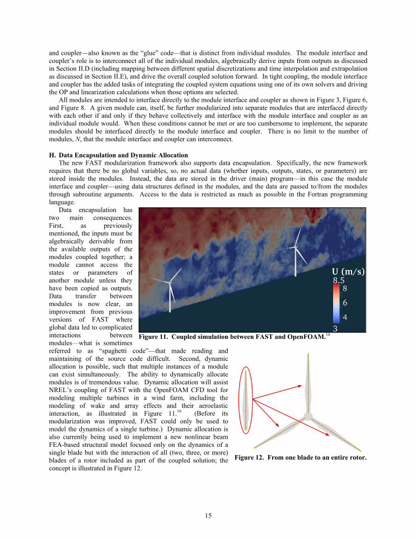
Data encapsulation has two main consequences. First, as previously mentioned, the inputs must be algebraically derivable from the available outputs of the modules coupled together; a module cannot access the states or parameters of another module unless they have been copied as outputs. Data transfer between modules is now clear, an improvement from previous versions of FAST where global data led to complicated interactions between modules—what is sometimes referred to as “spaghetti code”—that made reading and maintaining of the source code difficult. Second, dynamic allocation is possible, such that multiple instances of a module can exist simultaneously. The ability to dynamically allocate modules is of tremendous value. Dynamic allocation will assist NREL’s coupling of FAST with the OpenFOAM CFD tool for modeling multiple turbines in a wind farm, including the modeling of wake and array effects and their aeroelastic interaction, as illustrated in Figure 11.16 (Before its modularization was improved, FAST could only be used to model the dynamics of a single turbine.) Dynamic allocation is also currently being used to implement a new nonlinear beam FEA-based structural model focused only on the dynamics of a single blade but with the interaction of all (two, three, or more) blades of a rotor included as part of the coupled solution; the concept is illustrated in Figure 12.

Figure 11. Coupled simulation between FAST and OpenFOAM.16

Figure 12. From one blade to an entire rotor.

16

I. Save/Retrieve Capability The new FAST modularization framework also supports the ability to save the data across all modules at a given

instance during the course of a simulation. The data can be written to a file and retrieved later to continue the simulation starting from that point (i.e., restart). This save/retrieve feature is especially useful in the solution of computationally expensive systems to minimize the performance impact of HPC disruptions and/or the rerunning of common segments of the simulation.

III. Linearization As discussed in Section II.F, the tight coupling functionality of the new FAST modularization framework

supports OP determination and linearization of individual modules as well as of the overall coupled system; the linearization functionality is not available in loose coupling. This section summarizes the mathematical details of the linearization functionality for tight coupling, which is important to its understanding and proper application. The linearization mathematics is also illustrative of the coupling properties inherent in coupled system modeling within the new FAST modularization framework whether the underlying modules are fundamentally linear in nature or not.

A. Linearization of a Module A linear representation of a nonlinear system model is valid only for small deviations (perturbations) from an

OP. As discussed in Section II.F, an OP in the new FAST modularization framework can be defined by given ICs, a given time in the time-marching process, or an OP found through the OP determination calculation. Assuming OP values are given for the continuous states,

opx , discrete states, d

opx , inputs,

opu , and time,

opt , of a tightly

coupled module, Eqs. (1a), (1c), and (1d) can be used to calculate the OP values of the first time derivative of the continuous state,

opx , constraint states,

opz , and outputs,

opy . In this paper,

op denotes an OP value of a

variable or the evaluation of a function about the OP. Except for the OP time, op

t , each of these variables can be

perturbed (represented by Δ) about their respective OP values

op

x x x∆= + , d d d

opx x x∆= + ,

opu u u∆= + , (11a)

op

x x x∆= + , op

z z z∆= + , and op

y y y∆= + . (11b)

Substituting the expressions of Eq. (11) into Eq. (1), expanding as a Taylor-series approximation, and keeping only the linear terms (i.e., neglecting products of perturbations), it can be shown that the most general linearized form of Eq. (1) is represented mathematically as

DAC dx A x A x B u∆ ∆ ∆ ∆= + + , · (12a) [ ] [ ]d ADC d d ADC

t n t t n tx n 1 A x A x n B u

∆ ∆∆ ∆ ∆ ∆

= =+ = + + , and (12b)

DAC dy C x C x D u∆ ∆ ∆ ∆= + + , · (12c)

where

1

op

X X Z ZAx z z x

− ∂ ∂ ∂ ∂ = − ∂ ∂ ∂ ∂ , ·· (13a)

1

DACd d

op

X X Z ZAx z z x

− ∂ ∂ ∂ ∂ = − ∂ ∂ ∂ ∂ ,· ·· (13b)

17

1

op

X X Z ZBu z z u

− ∂ ∂ ∂ ∂ = − ∂ ∂ ∂ ∂ ,· ·· (13c)

1d d

ADC

op

X X Z ZAx z z x

− ∂ ∂ ∂ ∂ = − ∂ ∂ ∂ ∂ ,· ·· (13d)

1d d

dd d

op

X X Z ZAx z z x

− ∂ ∂ ∂ ∂ = − ∂ ∂ ∂ ∂ , (13e)

1d d

ADC

op

X X Z ZBu z z u

− ∂ ∂ ∂ ∂ = − ∂ ∂ ∂ ∂ , · (13f)

1

op

Y Y Z ZCx z z x

− ∂ ∂ ∂ ∂ = − ∂ ∂ ∂ ∂ , ·· (13g)

1

DACd d

op

Y Y Z ZCx z z x

− ∂ ∂ ∂ ∂ = − ∂ ∂ ∂ ∂ , and· (13h)

1

op

Y Y Z ZDu z z u

− ∂ ∂ ∂ ∂ = − ∂ ∂ ∂ ∂ . ·· (13i)

The perturbations of continuous states, Δx, are defined by the linear continuous-state equations of Eq. (12a) expressed as explicit first-order ODEs, where the RHS is the linearized form of the nonlinear continuous-state functions, X, of Eq. (1a). A is the continuous-state matrix, ADAC is the discrete-state matrix, and B is the input matrix of the linearized continuous-state equations. A is a square matrix with the number of rows and columns equal to the number of continuous states. The number of rows in ADAC equals the number of continuous states, and the number of columns equals the number of discrete states. The number of rows in B equals the number of continuous states, and the number of columns equals the number of inputs. These matrices, as well as the other matrices of Eq. (12), are time invariant and depend on the Jacobians of the functions in Eq. (1) as shown in Eq. (13) and discussed below. Like the continuous states themselves, the perturbations of continuous states are time dependent, so, Δx(t) is implied by Δx where t is time and x∆ is the first time derivative of Δx. And like the continuous-state equations themselves, the linear continuous-state equations are written in first-order form without loss of generality.***

***In the second-order example of footnote **, the linearized form of a second-order system without discrete and

constraint states, ( )q Q q,q,u,t= , is opop op

Q Q Qq q q uq q u

∆ ∆ ∆ ∆∂ ∂ ∂= + +∂ ∂ ∂

. The linearized first-order

form of this system can be realized by using q

xq

∆∆

∆

=

, with q

xq

∆∆

∆

=

,

op op

0 IA Q Q

q q

= ∂ ∂ ∂ ∂

, and

op

0B Q

u

= ∂ ∂

.

18

The perturbations of discrete states, Δxd, are defined by the linear discrete-state equations of (12b) expressed as explicit difference (recurrence) equations from step n to n 1+ , where the RHS is the linearized form of the nonlinear discrete-state functions, Xd, of Eq. (1b). Matrices AADC, Ad, and BADC are the continuous-state, discrete-state, and input matrices of the linearized discrete-state equations, respectively. While Ad is a square matrix with the number of rows and columns equal to the number of discrete states, the number of rows in AADC and BADC equals the number of discrete states, the number of columns in AADC equals the number of continuous states, and the number of columns in BADC equals the number of inputs. Like the discrete states and discrete-state functions themselves, the perturbations of discrete states and linearized discrete-state equations are evaluated only at discrete steps in time based on the fixed discrete time step (interval), Δt, which is greater than zero and the same for all discrete states of a given module. The ADC and DAC discussed in Section II.C also apply to the linearized system. (The superscripts ADC and DAC in the linearized system matrices indicate analog-to-digital and digital-to-analog conversions, respectively.) The OP time,

opt , need not be an integer multiple of the discrete time step, Δt. Even if discrete

states are present in a module, the perturbations of inputs, Δu, and outputs, Δy, are always expressed in continuous time.

The perturbations of outputs, Δy, are defined by the linear output equations of (12c) expressed explicitly in continuous time, where the RHS is the linearized form of the nonlinear output functions, Y, of Eq. (1d). Matrices C,

For the generalized form of Newton’s second law used by the existing structural module of FAST,

( ) ( ) ( )1Q q,q,u,t M q,u,t F q,q,u,t−= , it can be shown that 1 1

op op

Q F MM M Fq q q

− − ∂ ∂ ∂= − ∂ ∂ ∂

,

1

op op

Q FMq q

− ∂ ∂= ∂ ∂

, and 1 1

op op

Q F MM M Fu u u

− − ∂ ∂ ∂ = − ∂ ∂ ∂ . The standard generalized linear form of

Newton’s second law is typically written as uM q C q K q F u∆ ∆ ∆ ∆+ + = , where M is the generalized linear mass matrix, C is the generalized linear damping matrix (not to be confused with C from Eq. (13g)), K is the generalized linear stiffness matrix, and Fu is the generalized linear input forcing matrix. Relating these matrices to

the Jacobians of Q, it is clear that op

M M= , op

FCq

∂= −

∂ , 1

op

F MK M Fq q

− ∂ ∂= − − ∂ ∂

, and

u 1

op

F MF M Fu u

−∂ ∂ = − ∂ ∂ . It may be surprising that K doesn’t equal

op

Fq

∂−∂

and Fu doesn’t equal op

Fu

∂∂

,

which are common expressions. Noticing that { }1opop

M F q− = , it is seen that—because the mass matrix

depends on the displacements and control inputs (whereby op

M 0q

∂≠

∂ and

op

M 0u

∂≠

∂ in general)—the stiffness

and input forcing matrices are impacted by an OP that is not the static-equilibrium or steady-state condition (whereby

opq 0≠ ). While the linear model is still valid for the OP that is not the static-equilibrium or steady-state

condition about which the model was linearized, it is of less practical use than when op

FKq

∂= −

∂ and

u

op

FFu

∂=∂

. As such, it is usually important for the OP to be a static-equilibrium or steady-state condition

(whereby op

q 0= , op

FKq

∂= −

∂, and u

op

FFu

∂=∂

).

19

CDAC, and D are the continuous-state, discrete-state, and input-transmission matrices of the linearized output equations, respectively. The number of rows in C, CDAC, and D equals the number of outputs, and the number of columns in C, CDAC, and D equals the number of continuous states, discrete states, and inputs, respectively. The input-transmission matrix, D, is present if the module has direct feedthrough of input to output.

All matrices of Eq. (12) depend on the Jacobians of the functions in Eq. (1), as shown in Eq. (13). To be able to form the linearized system, a tightly coupled module must be able to calculate and return the OP values of the 16

Jacobian matrices, op

Xx

∂∂

, dop

Xx∂∂

, op

Xz

∂∂

, op

Xu

∂∂

, d

op

Xx

∂∂

, d

dop

Xx

∂∂

, d

op

Xz

∂∂

, d

op

Xu

∂∂

, op

Zx

∂∂

, dop

Zx∂∂

,

op

Zz

∂∂

, op

Zu∂∂

, op

Yx

∂∂

, dop

Yx∂∂

, op

Yz

∂∂

, and op

Yu

∂∂

. These Jacobian matrices—and thus all matrices of Eq.

(12)—can be functions of the OP values of the continuous states, op

x , discrete states, d

opx , constraint states,

opz , inputs,

opu , and time,

opt , (and, of course, are characterized by the parameters evaluated at the OP time,

( )opp t ), but are themselves time invariant. (If the nonlinear system of Eq. (1) was characterized with time-

dependent parameters, p(t), the parameters are effectively replaced with time-invariant parameters, ( )opp t , in the

linearized system of Eq. (12).) Module developers can choose to compute these Jacobian matrices in the module either numerically (e.g., through a central-difference perturbation technique) or analytically. The analytical approach is preferred when practical because it is more accurate than numerical approaches, whose accuracy is dictated by the perturbation size of the numerical technique.

The constraint-state (algebraic) equations have been eliminated from the linearized system of Eq. (12) because once linearized, the constraint-state equations can be easily solved for the perturbations of constraint states, Δz. The perturbations of constraint states are then substituted into the remaining equations of Eq. (12), essentially eliminating Δz as a separate variable. By eliminating the constraint-state equations, each of the matrices of Eq. (12) depend on Jacobians that are taken with respect to the constraint states and of the Jacobians of the constraint-state functions as shown in Eq. (13). The existence of the matrix inverse of the Jacobian of the constraint-state functions

with respect to constraint states, 1Z

z

−∂ ∂

, resulted from the limitation in tight coupling that the constraints must be

of index 1, as discussed in Section II.C. Equation (12) is readily identifiable as a general state-space representation of a linear time-invariant (LTI)

system with a combination of continuous and discrete states (i.e., a “sampled” or “hybrid” LTI system). A linearized system with continuous states but without discrete states reduces to a standard continuous LTI state-space model characterized by matrices A, B, C, and D. A linearized system with discrete states but without continuous states reduces to a discrete LTI state-space model, but with continuous inputs and outputs, characterized by matrices Ad, BADC, CDAC, and D.

It is usually important for the OP to be a static-equilibrium or steady-state condition. An OP that is not the static-equilibrium or steady-state condition may have an undesirable effect on the linear system matrices, as discussed in footnote ***. But, if the system implemented in a module was naturally linear to begin with, the linearization process will simply result in the same linear system regardless of the OP.

B. Linearization of the Overall Coupled System Once an OP has been determined across all coupled modules and each individual module has been linearized as

discussed in Section III.A, linearization of the overall coupled system is possible. Given N total number of linearized modules coupled together, the perturbations of inputs and outputs can be combined into vectors across all modules, just as the inputs and outputs from each individual module were combined across all modules in Eq. (2),

20

( )

( )

( )

1

2

N

u

uu

u

∆

∆∆

∆

=

and

( )

( )

( )

1

2

N

y

yy

y

∆

∆∆

∆

=

. (14)

Similar to how Eq. (1) was linearized to form Eq. (12), the input-output transformation functions, U, of Eq. (3) can be linearized

op op

U U0 u yu y

∆ ∆∂ ∂= +∂ ∂

with op

U 0u

∂≠

∂ , (15)

where the Jacobian matrices Uu

∂∂

and

Uy

∂∂

—written out in Eq. (10)—have been

evaluated at the OP and are time invariant. Equation (15) can be used to solve for the perturbations of inputs given the perturbations of outputs across all coupled modules.

It is convenient to see the effect of externally provided inputs on the linear coupled system model. For example, the linear model of the coupled system could be used as a linear plant model from which to develop an advanced linear state-space-based controller, where the linear plant model includes the coupled dynamics of wind turbine aero-elastics plus the dynamics of a baseline controller; it would be useful in this case to see the effect of additional control inputs on top of the baseline control signals in the linear system response. To accommodate this feature, the input perturbations derived from Eq. (15) are augmented with additional (but not quantified) input perturbations, Δu+, before being sent to each module. The concept is illustrated in Figure 13, which follows the organization of Figure 8 but uses the nomenclature of the matrices from the linearized state, output, and input equations and perturbations of inputs and outputs. Mathematically,

u u u∆ ∆ ∆ += + , (16)

where u∆ is a dummy variable representing the input perturbations derived from Eq. (15), Δu+ are the additional input perturbations, and Δu are the actual input perturbations sent to each module. All of the input perturbations of Eq. (16) are vectors combining the perturbations across all coupled modules. The perturbations of states can also be combined into vectors across all modules

+

( )

( ) ( ) ( ) ( ) ( )

( ) ( ) ( )

( ) ( ) ( ) ( )

( )

( ) ( ) ( ) ( ) ( )

( ) ( ) ( )

( ) ( ) ( ) ( )

( )

( ) ( ) ( ) ( ) ( )

( ) ( ) ( )

( ) ( ) ( ) ( )

1

1 1 1 DAC 1 1

ADC 1 d 1 ADC 1

1 1 DAC 1 1

2

2 2 2 DAC 2 2op

ADC 2 d 2 ADC 2

2 2 DAC 2 2op

N

N N N DAC N N

ADC N d N ADC N

N N DAC N N

u

u u A ,A ,B ,

A ,A ,B ,

y C ,C ,D

uU ,u u u A ,A ,B ,U A ,A ,B ,y y C ,C ,D

u

u u A ,A ,B

A ,A ,B ,

y C ,C ,D

y

∆

∆ ∆

∆

∆

∆ ∆

∆

∆

∆ ∆

∆

∆

+

+

+

∂∂

∂∂

+

+

Figure 13. Coupling of N linearized modules.

21

( )

( )

( )

1

2

N

u

uu

u

∆

∆∆

∆

+

++

+

=

,

( )

( )

( )

1

2

N

x

xx

x

∆

∆∆

∆

=

, and

( )

( )

( )

d 1

d 2d

d N

x

xx

x

∆

∆∆

∆

=

. (17)

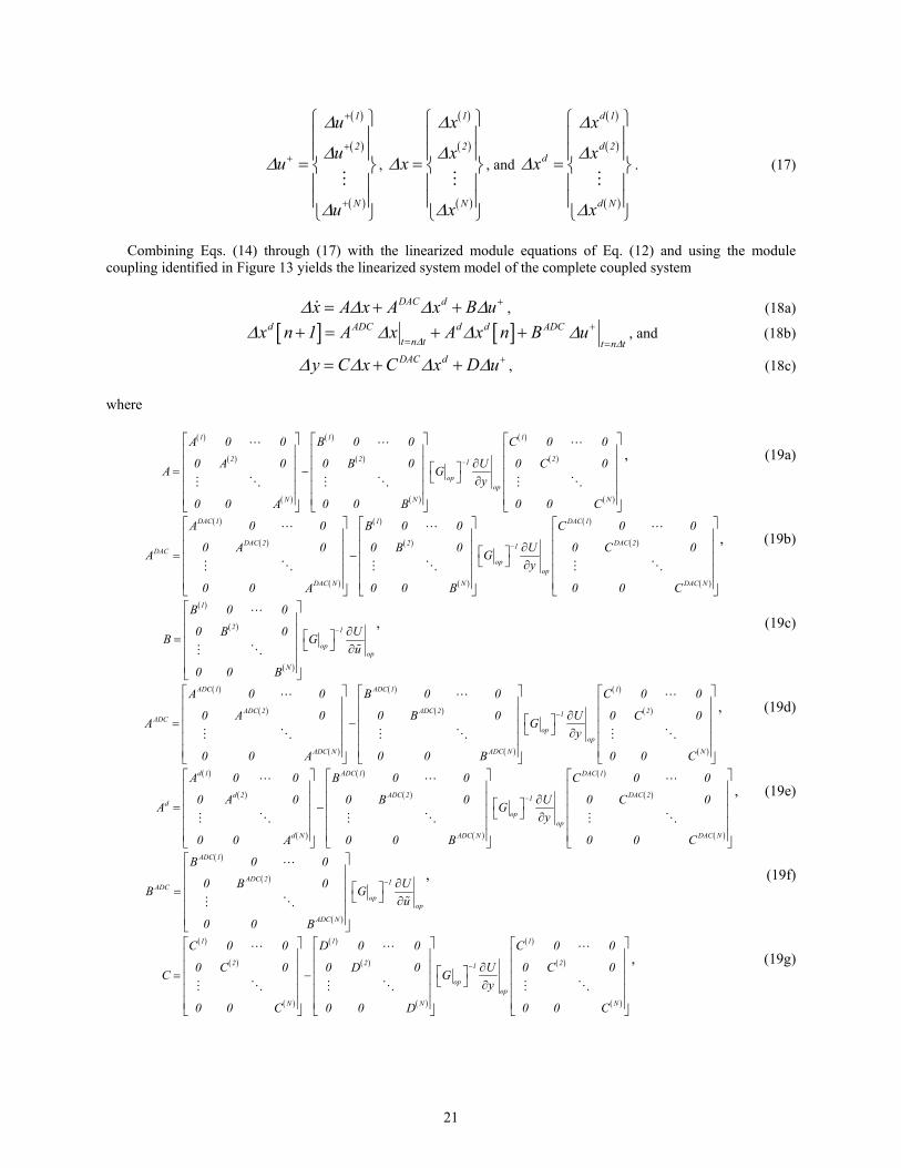
Combining Eqs. (14) through (17) with the linearized module equations of Eq. (12) and using the module coupling identified in Figure 13 yields the linearized system model of the complete coupled system

DAC dx A x A x B u∆ ∆ ∆ ∆ += + + , · (18a)

[ ] [ ]d ADC d d ADCt n t t n t

x n 1 A x A x n B u∆ ∆

∆ ∆ ∆ ∆ += =

+ = + + , and (18b)

DAC dy C x C x D u∆ ∆ ∆ ∆ += + + , · (18c)

where

( )

( )

( )

( )

( )

( )

( )

( )

( )

1 1 1

2 2 21

opop

N N N

A 0 0 B 0 0 C 0 0

U0 A 0 0 B 0 0 C 0A Gy

0 0 A 0 0 B 0 0 C

−

∂ = − ∂

,· ·· (19a)

( )

( )

( )

( )

( )

( )

( )

( )

( )

DAC 1 1 DAC 1

DAC 2 2 DAC 21DAC

opop

DAC N N DAC N

A 0 0 B 0 0 C 0 0

U0 A 0 0 B 0 0 C 0A Gy

0 0 A 0 0 B 0 0 C

−

∂ = − ∂

, ·· (19b)

( )

( )

( )

1

2 1

opop

N

B 0 0

U0 B 0B Gu

0 0 B

−

∂ = ∂

,· ·· (19c)

( )

( )

( )

( )

( )

( )

( )

( )

( )

ADC 1 ADC 1 1

ADC 2 ADC 2 21ADC

opop

ADC N ADC N N

A 0 0 B 0 0 C 0 0

U0 A 0 0 B 0 0 C 0A Gy

0 0 A 0 0 B 0 0 C

−

∂ = − ∂

,· · ·· (19d)

( )

( )

( )

( )

( )

( )

( )

( )

( )

d 1 ADC 1 DAC 1

d 2 ADC 2 DAC 21d

opop

d N ADC N DAC N

A 0 0 B 0 0 C 0 0

U0 A 0 0 B 0 0 C 0A Gy

0 0 A 0 0 B 0 0 C

−

∂ = − ∂

,·· (19e)

( )

( )

( )

ADC 1

ADC 2 1ADC

opop

ADC N

B 0 0

U0 B 0B Gu

0 0 B

−

∂ = ∂

, · (19f)

( )

( )

( )

( )

( )

( )

( )

( )

( )

1 1 1

2 2 21

opop

N N N

C 0 0 D 0 0 C 0 0

U0 C 0 0 D 0 0 C 0C Gy

0 0 C 0 0 D 0 0 C

−

∂ = − ∂

,· ·· (19g)

22

( )

( )

( )

( )

( )

( )

( )

( )

( )

DAC 1 1 DAC 1

DAC 2 2 DAC 21DAC

opop

DAC N N DAC N

C 0 0 D 0 0 C 0 0

U0 C 0 0 D 0 0 C 0C Gy

0 0 C 0 0 D 0 0 C

−

∂ = − ∂

, and· (19h)

( )

( )

( )

1

2 1

opop

N

D 0 0

U0 D 0D Gu

0 0 D

−

∂ = ∂

.· ·· (19i)

Equation (18) is the linearized form of the nonlinear coupled system equations of Eq. (7) with additional input perturbations, Δu+. Similar to how the constraint-state equations have been eliminated from the linearized system of Eq. (12), the inputs that act as additional constraint states in Eq. (7c) have been eliminated from Eq. (18). This was possible because, once linearized, the additional constraint-state equations (i.e., the linearized input-output transformation equations) can be easily solved, essentially eliminating u∆ as separate variables. Eliminating u∆ causes each of the matrices of Eq. (19) to depend on the matrix

opG , which is the matrix G from Eq. (9) evaluated

at the OP,

( )

( )

( )

1

2

opop op

N

D 0 0

U U 0 D 0Gu y

0 0 D

∂ ∂ = + ∂ ∂

with

opG 0≠ . (20)

Although they appear nearly identical, Eq. (18) should not be confused with Eq. (12). Equation (18) applies to the coupled linear solution of all modules whereas Eq. (12) applies only to an individual linearized module. Effectively, the coupling illustrated in Figure 13 has been reduced to the system illustrated in Figure 14. Please note that if the discrete time step (interval), Δt, differs between individual modules, separate discrete-state-perturbation and linear discrete-state-equation groupings are needed, even though they have been shown grouped together in Eq. (18).

Equation (19) shows that all matrices of Eq. (18) are derived from the linearized input-output transformation functions evaluated at the OP from Eq. (15) and from the linearized matrices of each individual module from Eq. (13). So, once all individual modules have been linearized, the linearized system model of the complete coupled system can be assembled. All matrices of Eq. (18) are time invariant.

Like Eq. (12), Eq. (18) is readily identifiable as a general state-space representation of an LTI system with a combination of continuous and discrete states (i.e., a “sampled” or “hybrid” LTI system). A coupled linearized system with continuous states but without discrete states reduces to a standard continuous LTI state-space model characterized by matrices A, B, C, and D. A coupled linearized system with discrete states but without continuous states reduces to a discrete LTI state-space model, but with continuous inputs and outputs, characterized by matrices Ad, BADC, CDAC, and D.

The matrices of the linearized coupled system model are very illustrative of the coupling properties inherent in

coupled system modeling. While many of the matrices in Eq. (19) are block-diagonal, matrices 1

opG

− ,

op

Uu

∂∂

,

DAC

ADC d ADC

DAC

u

A,A ,B,A ,A ,B ,C,C ,D

y

∆

∆

+

Figure 14. Effective coupled linear system.

23

and op

Uy

∂∂

may be full in general, so, the matrices of the linearized coupled system model may also be full in

general. The module-to-module coupling is apparent.†††

†††In the two module example of footnotes †† and ‡‡, ( )

( )

2

op 1

I DG

D I

−=

− with ( ) ( )1 2

opG I D D 0= − ≠ .

The matrices of the linearized coupled system model for this two module example are given below and clearly show off-diagonal terms and coupling between the two modules:

( ) ( ) ( ) ( ) ( ) ( ) ( ) ( ) ( ) ( ) ( ) ( ) ( ) ( )

( ) ( ) ( ) ( ) ( ) ( ) ( ) ( ) ( ) ( )

1 11 1 2 1 2 1 1 2 1 2 1 2 1 2

1 12 1 2 1 2 2 1 2 1 2

A B D I D D C B C B D I D D D CA

B I D D C A B I D D D C

− −

− −

+ − + − = − + −

,

( ) ( ) ( ) ( ) ( ) ( ) ( ) ( ) ( ) ( ) ( ) ( ) ( ) ( )

( ) ( ) ( ) ( ) ( ) ( ) ( ) ( ) ( ) ( )

1 1DAC 1 1 2 1 2 DAC 1 1 DAC 2 1 2 1 2 1 DAC 2

DAC1 12 1 2 DAC 1 DAC 2 2 1 2 1 DAC 2

A B D I D D C B C B D I D D D CA

B I D D C A B I D D D C

− −

− −

+ − + − = − + −

,

( ) ( ) ( ) ( ) ( ) ( ) ( ) ( ) ( ) ( )

( ) ( ) ( ) ( ) ( ) ( ) ( )

1 11 1 2 1 2 1 1 2 1 2

1 12 1 2 1 2 1 2

B B D I D D D B D I D DB

B I D D D B I D D

− −

− −

+ − − = − −

,

( ) ( ) ( ) ( ) ( ) ( ) ( ) ( ) ( ) ( ) ( ) ( ) ( ) ( )

( ) ( ) ( ) ( ) ( ) ( ) ( ) ( ) ( ) ( )

1 1ADC 1 ADC 1 2 1 2 1 ADC 1 2 ADC 1 2 1 2 1 2

ADC1 1ADC 2 1 2 1 ADC 2 ADC 2 1 2 1 2

A B D I D D C B C B D I D D D CA

B I D D C A B I D D D C

− −

− −

+ − + − = − + −

,

( ) ( ) ( ) ( ) ( ) ( ) ( ) ( ) ( ) ( ) ( ) ( ) ( ) ( )

( ) ( ) ( ) ( ) ( ) ( ) ( ) ( ) ( ) ( )

1 1d 1 ADC 1 2 1 2 DAC 1 ADC 1 DAC 2 ADC 1 2 1 2 1 DAC 2

d1 1ADC 2 1 2 DAC 1 d 2 ADC 2 1 2 1 DAC 2

A B D I D D C B C B D I D D D CA

B I D D C A B I D D D C

− −

− −

+ − + − = − + −

,

( ) ( ) ( ) ( ) ( ) ( ) ( ) ( ) ( ) ( )

( ) ( ) ( ) ( ) ( ) ( ) ( )

1 1ADC 1 ADC 1 2 1 2 1 ADC 1 2 1 2

ADC1 1ADC 2 1 2 1 ADC 2 1 2

B B D I D D D B D I D DB

B I D D D B I D D

− −

− −

+ − − = − −

,

( ) ( ) ( ) ( ) ( ) ( ) ( ) ( ) ( ) ( ) ( ) ( ) ( ) ( )

( ) ( ) ( ) ( ) ( ) ( ) ( ) ( ) ( ) ( )

1 11 1 2 1 2 1 1 2 1 2 1 2 1 2

1 12 1 2 1 2 2 1 2 1 2

C D D I D D C D C D D I D D D CC

D I D D C C D I D D D C

− −

− −

+ − + − = − + −

,

( ) ( ) ( ) ( ) ( ) ( ) ( ) ( ) ( ) ( ) ( ) ( ) ( ) ( )

( ) ( ) ( ) ( ) ( ) ( ) ( ) ( ) ( ) ( )

1 1DAC 1 1 2 1 2 DAC 1 1 DAC 2 1 2 1 2 1 DAC 2

DAC1 12 1 2 DAC 1 DAC 2 2 1 2 1 DAC 2

C D D I D D C D C D D I D D D CC

D I D D C C D I D D D C

− −

− −

+ − + − = − + −

, and

( ) ( ) ( ) ( ) ( ) ( ) ( ) ( ) ( ) ( )

( ) ( ) ( ) ( ) ( ) ( ) ( )

1 11 1 2 1 2 1 1 2 1 2

1 12 1 2 1 2 1 2

D D D I D D D D D I D DD

D I D D D D I D D

− −

− −

+ − − = − −

.

In the example of footnote §§ where the output of one of the modules is the conjugate quantity of the output of the

other module, ( )1D 0= , so all terms in the equations above involving ( ) ( ) 11 2I D D−

− reduce to I, and the

24

The continuous-state matrix for the linearized continuous-state equations of the coupled system, A, depends on the continuous-state and input matrices for the linearized continuous-state equations from each individual module, the continuous-state and input-transmission matrices for the linearized output equations from each individual module, and the linearized input-output transformation functions evaluated at the OP, as shown in Eq. (19a) and Eq. (20). These dependencies are similar for the discrete-state matrix for the linearized continuous-state equations of the coupled system, ADAC; the continuous-state and discrete-state matrices for the linearized discrete-state equations of the coupled system, AADC and Ad, respectively; and the continuous-state and discrete-state matrices for the linearized output equations of the coupled system, C and CDAC, respectively. The input matrix for the linearized continuous-state equations of the coupled system, B, depends on the input matrix for the linearized continuous-state equations from each module, the input-transmission matrices for the linearized output equations from each individual module, and the linearized input-output transformation functions evaluated at the OP, as shown in Eq. (19c) and Eq. (20). These dependencies are similar for the input matrix for the linearized discrete-state equations of the coupled system, BADC, and input-transmission matrix for the linearized output equations of the coupled system, D. It is interesting to note that the input-transmission matrices of each individual module, D, impact all matrices of the linearized coupled system as illustrated in footnote †††, further highlighting the importance of the role played by direct feedthrough of input to output in the coupled system response.

IV. Conclusion NREL recently has put considerable effort into improving the overall modularity of its FAST wind turbine aero-

hydro-servo-elastic tool to (1) improve the ability to read, implement, and maintain source code; (2) increase module sharing and shared code development across the wind community; (3) improve numerical performance and robustness; and (4) greatly enhance flexibility and expandability to enable further developments of functionality without the need to recode established modules. The new FAST modularization framework supports module-independent inputs, outputs, states, and parameters; states in continuous-time, discrete-time, and constraint form; loose and tight coupling; independent time and spatial discretizations; time marching, operating-point determination, and linearization; data encapsulation; dynamic allocation; and save/retrieve capability. This paper explains the features of the new framework, as well as the concepts and mathematical background needed to understand and apply them correctly. Table 3 summarizes the features of the new FAST modularization framework dependent on whether the modules are loosely or tightly coupled.

It is envisioned that the new modularization framework will transform FAST into a powerful, flexible, and robust wind turbine modeling tool with a large number of developers and a range of modeling fidelities across the aerodynamic, hydrodynamic, servo-dynamic, and structural-dynamic components.

At its core, the new FAST modularization framework is a means by which various mathematical systems are implemented in distinct modules and interconnected to solve for the global, coupled, dynamic response of a system. While the intent was to establish a framework to better model wind turbines, in reality, the new FAST modularization framework is quite general and could be applied to systems other than wind turbines, as long as the mathematical models of those systems are implemented in modules developed under the same framework.

Future Work Work is ongoing to convert the existing modules of FAST, including AeroDyn and HydroDyn, to the format

required of the new modularization framework, including the data structures and interface procedures. The loose coupling functionality and mesh library will be completed first, followed by the tight coupling functionality for time

matrices of the linearized coupled system model simplify greatly as follows:

( ) ( ) ( ) ( ) ( ) ( )

( ) ( ) ( )

1 1 2 1 1 2

2 1 2

A B D C B CA

B C A

+=

, ( ) ( ) ( ) ( ) ( ) ( )

( ) ( ) ( )

DAC 1 1 2 DAC 1 1 DAC 2DAC

2 DAC 1 DAC 2

A B D C B CA

B C A

+=

, ( ) ( ) ( )

( )

1 1 2

2

B B DB

0 B

=

,

( ) ( ) ( ) ( ) ( ) ( )

( ) ( ) ( )

ADC 1 ADC 1 2 1 ADC 1 2ADC

ADC 2 1 ADC 2

A B D C B CA

B C A

+=

, ( ) ( ) ( ) ( ) ( ) ( )

( ) ( ) ( )

d 1 ADC 1 2 DAC 1 ADC 1 DAC 2d

ADC 2 DAC 1 d 2

A B D C B CA

B C A

+=

,

( ) ( ) ( )

( )

ADC 1 ADC 1 2ADC

ADC 2

B B DB

0 B

=

, ( )

( ) ( ) ( )

1

2 1 2

C 0C

D C C

=

, ( )

( ) ( ) ( )

DAC 1DAC

2 DAC 1 DAC 2

C 0C

D C C

=

, and ( )2

0 0D

0 D

=

.

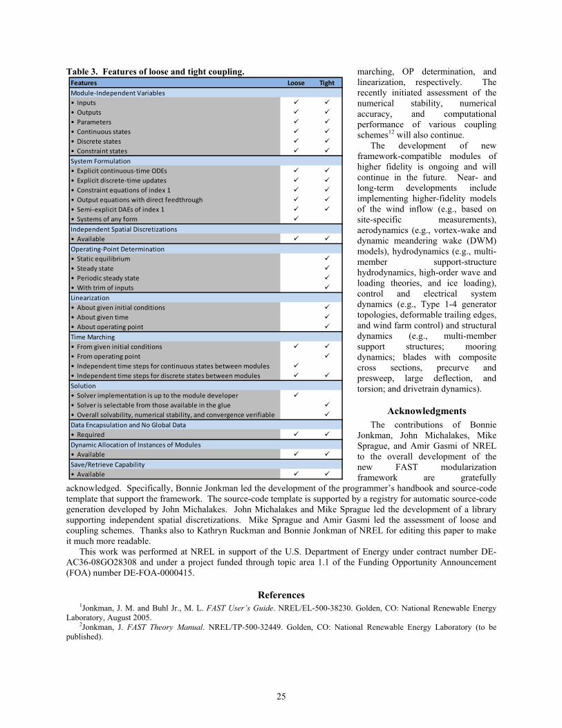
25

marching, OP determination, and linearization, respectively. The recently initiated assessment of the numerical stability, numerical accuracy, and computational performance of various coupling schemes12 will also continue.

The development of new framework-compatible modules of higher fidelity is ongoing and will continue in the future. Near- and long-term developments include implementing higher-fidelity models of the wind inflow (e.g., based on site-specific measurements), aerodynamics (e.g., vortex-wake and dynamic meandering wake (DWM) models), hydrodynamics (e.g., multi-member support-structure hydrodynamics, high-order wave and loading theories, and ice loading), control and electrical system dynamics (e.g., Type 1-4 generator topologies, deformable trailing edges, and wind farm control) and structural dynamics (e.g., multi-member support structures; mooring dynamics; blades with composite cross sections, precurve and presweep, large deflection, and torsion; and drivetrain dynamics).

Acknowledgments The contributions of Bonnie

Jonkman, John Michalakes, Mike Sprague, and Amir Gasmi of NREL to the overall development of the new FAST modularization framework are gratefully

acknowledged. Specifically, Bonnie Jonkman led the development of the programmer’s handbook and source-code template that support the framework. The source-code template is supported by a registry for automatic source-code generation developed by John Michalakes. John Michalakes and Mike Sprague led the development of a library supporting independent spatial discretizations. Mike Sprague and Amir Gasmi led the assessment of loose and coupling schemes. Thanks also to Kathryn Ruckman and Bonnie Jonkman of NREL for editing this paper to make it much more readable.

This work was performed at NREL in support of the U.S. Department of Energy under contract number DE-AC36-08GO28308 and under a project funded through topic area 1.1 of the Funding Opportunity Announcement (FOA) number DE-FOA-0000415.

References 1Jonkman, J. M. and Buhl Jr., M. L. FAST User’s Guide. NREL/EL-500-38230. Golden, CO: National Renewable Energy

Laboratory, August 2005. 2Jonkman, J. FAST Theory Manual. NREL/TP-500-32449. Golden, CO: National Renewable Energy Laboratory (to be

published).

Table 3. Features of loose and tight coupling. Features Loose TightModule-Independent Variables• Inputs • Outputs • Parameters • Continuous states • Discrete states • Constraint states

System Formulation• Explicit continuous-time ODEs • Explicit discrete-time updates • Constraint equations of index 1 • Output equations with direct feedthrough • Semi-explicit DAEs of index 1 • Systems of any form

Independent Spatial Discretizations• Available

Operating-Point Determination• Static equilibrium • Steady state • Periodic steady state • With trim of inputs

Linearization• About given initial conditions • About given time • About operating point

Time Marching• From given initial conditions • From operating point • Independent time steps for continuous states between modules • Independent time steps for discrete states between modules

Solution• Solver implementation is up to the module developer • Solver is selectable from those available in the glue • Overall solvability, numerical stability, and convergence verifiable

Data Encapsulation and No Global Data• Required

Dynamic Allocation of Instances of Modules• Available

Save/Retrieve Capability• Available

26

3Laino, D. J. and Hansen, A. C. User’s Guide to the Wind Turbine Dynamics Aerodynamics Computer Software AeroDyn. Salt Lake City, UT: Windward Engineering LLC. Prepared for the National Renewable Energy Laboratory under Subcontract No. TCX-9-29209-01, December 2002.

4Moriarty, P. J. and Hansen, A. C. AeroDyn Theory Manual. NREL/EL-500-36881. Golden, CO: National Renewable Energy Laboratory, December 2005.

5Jonkman, J. M. Dynamics Modeling and Loads Analysis of an Offshore Floating Wind Turbine. Ph.D. Thesis. Department of Aerospace Engineering Sciences, University of Colorado, Boulder, CO, 2007; NREL/TP-500-41958. Golden, CO: National Renewable Energy Laboratory.

6Jonkman, J. M. “Dynamics of Offshore Floating Wind Turbines—Model Development and Verification.” Wind Energy. Vol. 12, No. 5, July 2009, pp. 459-492; NREL/JA-500-45311. Golden, CO: National Renewable Energy Laboratory; DOI: 10.1002/we.347.

7Web page: http://wind.nrel.gov/designcodes/ (accessed June 1, 2012). 8Laino, D. J. and Hansen, A. C. User’s Guide to the Computer Software Routines AeroDyn Interface for ADAMS®. Salt Lake

City, UT: Windward Engineering LLC. Prepared for the National Renewable Energy Laboratory under Subcontract No. TCX-9-29209-01, September 2001.

9van Garrel, A. Development of a Wind Turbine Aerodynamics Simulation Module. ECN-C--03-079. Petten, The Netherlands: Energy research Centre of the Netherlands, August 2003.

10Jonkman, B. J.; Michalakes, J.; Jonkman, J. M.; Buhl Jr., M. L.; Platt, A.; and Sprague, M. A. NWTC Programmer’s Handbook: A Guide for Software Development within the FAST Computer-Aided Engineering Tool. Golden, CO: National Renewable Energy Laboratory (to be published).

11Cordle, A. and Jonkman, J. “State of the Art in Floating Wind Turbine Design Tools.” The Proceedings of the Twenty-First (2011) International Offshore and Polar Engineering Conference, 19–24 June 2011, Maui, HI [CD-ROM]. Vol. 1, pp. 367-374. 2011-TPC-1059. Cupertino, CA: International Society of Offshore and Polar Engineers (ISOPE), June 2011; NREL/CP-500-50543. Golden, CO: National Renewable Energy Laboratory.

12Gasmi, A.; Sprague, M. A.; Jonkman, J. M.; and Jones, W. B. “Numerical Stability and Accuracy of Temporally Coupled Multi-Physics Modules in Wind-Turbine CAE Tools.” 51st AIAA Aerospace Sciences Meeting including the New Horizons Forum and Aerospace Exposition, 7–10 January 2013, Grapevine (Dallas/Ft. Worth Region), TX. Reston, VA: American Institute of Aeronautics and Astronautics, January 2013 (to be published); NREL/CP-500-57298. Golden, CO: National Renewable Energy Laboratory.

13Bendtsen, C. and Thomsen, P. G., Numerical Solution of Differential Algebraic Equations. IMM-REP-1999-8. Lyngby, Denmark: Technical University of Denmark, May 1999.

14Shampine, L. F.; Reichelt, M. W.; and Kierzenka, J. A., “Solving Index-1 DAEs in MATLAB and Simulink.” SIAM Review, Vol. 41, No. 3, 1997, pp. 538-552.

15Felippa, C. A. Introduction to Finite Element Methods, Boulder, CO: University of Colorado, Fall 2004. 16Lee, S.; Churchfield, M.; Moriarty, P.; Jonkman, J.; and Michalakes, J. “Atmospheric and Wake Turbulence Impacts on

Wind Turbine Fatigue Loadings.” 50th AIAA Aerospace Sciences Meeting including the New Horizons Forum and Aerospace Exposition, 9–12 January 2012, Nashville, TN [online proceedings]. URL: http://pdf.aiaa.org/getfile.cfm?urlX=527I%276D%26X%5BRO%2FSPWIP4S%5EQ%3AG%224%3A%5C%25%0A. AIAA-2012-0540. Reston, VA: American Institute of Aeronautics and Astronautics, January 2012; NREL/CP-500-53567. Golden, CO: National Renewable Energy Laboratory.