New mapping techniques to estimate the preferential loss

HYDROLOGICAL PROCESSESHydrol. Process. (2015)Published online in Wiley Online Library(wileyonlinelibrary.com) DOI: 10.1002/hyp.10582

New mapping techniques to estimate the preferential loss ofsmall wetlands on prairie landscapes

J. N. Serran1 and I. F. Creed2*1 Department of Geography, Western University, 1151 Richmond Street, London, Ontario, Canada, N6A 5B72 Department of Biology, Western University, 1151 Richmond Street, London, Ontario, Canada, N6A 5B7

*CUnE-m

Co

Abstract:

Reliable estimates of wetland loss require improved wetland inventories and effective monitoring programmes. The PrairiePothole Region of North America is experiencing rapid urban, agricultural and economic development, which places wetlands atrisk, especially small geographically isolated wetlands. This loss is concomitant with a loss of ecosystem services. To improveupon current wetland inventories, a method for mapping wetlands using an automated object-based approach was developed fora regional watershed in Alberta. The method improves upon existing wetland mapping methods by effectively mapping smallwetlands and better capturing the convolution of wetland edges. This approach uses digital terrain objects derived from lightdetection and ranging data, from which 130 157 wetlands were identified. Wetland loss estimates (% number and % area) wereobtained by applying a wetland area versus frequency power-law function to the wetland inventory. We estimated a 16.2%historic loss of wetland number and a 2.6% loss of wetland area, with the size of these lost wetlands <0.04 ha. The improvedtechniques for mapping wetland loss and estimating wetland loss provide a more accurate representation of the magnitude ofwetland loss in the Prairie Pothole Region. Copyright © 2015 John Wiley & Sons, Ltd.

KEY WORDS mapping techniques; wetland; wetland loss; power-law; area; frequency

Received 5 February 2015; Accepted 16 June 2015

INTRODUCTION

The Prairie Pothole Region is a large physiographic regionextending from the Prairie Provinces of Canada into theNorthern Great Plains of the USA. This unique landscape isdue to the deposition of glacial till and the forces of meltingice andglacial scouring during the last glacial period (Kantrudet al., 1989). Glacial retreat left the landscape pockmarkedwith millions of small typically disconnected depressions or‘potholes’. These potholes are isolated from the surface waternetwork, and thus are known as geographically isolatedwetlands (Tiner, 2003). It is estimated that up to 70% ofwetlands have been lost or degraded in areas near theCanada–US border (Warner and Asada, 2006). These lossesare attributed to increasing urban and agricultural develop-ment pressures causing wetlands to be dredged and drainedfor the purposes of economic expansion (Davidson, 2014). Inthe US portion of the Prairie Pothole Region, 95% of the lossof wetlands to uplands from 1997–2009 occurred as a resultof agricultural development (Dahl, 2014).When these wetlands are lost, associated functions are

lost as well (Naugle et al., 2001; Zedler and Kercher,

orrespondence to: Irena F. Creed, Department of Biology, Westerniversity, London, ON, Canada, N6A 5B7.ail: [email protected]

pyright © 2015 John Wiley & Sons, Ltd.

2005). A common misconception about prairie potholes isthat the lack of surface water and connectivity to thesurface water network indicates that these wetlandsfunction less than more permanent wetlands and thereforeprovide fewer ecosystem services (e.g. Semlitsch andBodie, 1998; McLaughlin et al., 2014). Although prairiepotholes are disconnected from the surface water network,they have been found to have important contributions to thegroundwater system via wetland-groundwater interactionsand can be either groundwater sinks or sources (McLaughlinet al., 2014). In addition, prairie potholes are consideredimportant biogeochemical reactors within watersheds asthey remove nutrients such as nitrogen (Crumpton andGoldsborough, 1998; Lane et al., 2015) and phosphorus(Reddy et al., 1999; Craft and Casey, 2000; Dunne et al.,2007) and sequester carbon (Badiou et al., 2011; Creedet al., 2013) at rates comparable with or higher thanconnected wetlands. Prairie potholes provide ecosystemservices such as the desynchronization and attenuation offloodwater before it enters the surface water network (Laneand D’Amico, 2010; Pomeroy et al., 2014) and theimprovement of downstream water quality (Westbrooket al., 2011).Wetlands need to be managed effectively in a manner

that balances the needs for economic development and thepreservation of ecological services provided by wetlands.

J. N. SERRAN AND I. F. CREED

Successful wetland management requires accurate wetlandinventories to estimate rates of change in wetland numberand area and to understand the spatial and temporalpatterns of these changes (Li and Chen, 2005). Unfortu-nately, current wetland inventories are often incomplete,time-consuming to create, non-standardized and out of date(Baker et al., 2006). National wetland data exist for bothCanada [CanadianWetland Inventory (CWI)] and the USA[National Wetland Inventory (NWI)]. However, the size ofthe minimum mapping unit (MMU) for these inventoriesranges from 0.02 (manually derived) to 1 ha for the CWI(Fournier et al., 2007) and from 0.4–1.2 ha for the NWI(Martin et al., 2012). These current wetland inventories aretoo coarse in resolution to be useful in the Prairie PotholeRegion (Finlayson et al., 1999; Clare and Creed, 2013; Naet al., 2013; Davidson, 2014) where the majority of prairiepotholes are smaller than 1 ha (van der Valk and Pederson,2003). It is difficult to effectively manage and obtainestimates of the loss of small wetlands when all wetlandsare not captured (Na et al., 2013). Small (<1ha) wetlandsare vulnerable to continued loss on prairie landscapes, inpart because they are often not included in wetlandinventories.Wetland managers need high-resolution wetland map-

ping techniques that are sensitive to the detection of smallwetlands and simple standardized methods to estimate theloss of all sizes of wetlands. Several challenges exist whencreating accurate and automated wetland inventories,including the lack of techniques to capture their size andshape because wetlands on prairie landscapes often holdwater for only short periods of time, such as after the springmelt or during summer storms (Tiner, 2003). The com-plexity of the edges of isolated wetland basins is oftendifficult to capture in wetland inventories because of coarseresolution data inputs and dynamic water levels. Edges arefrequently under-estimated or over-estimated when wet-lands are digitized manually. It is important to capture theshape of wetland boundaries as wetland morphometryaffects wetland function. For example, the convolutednessof an isolated wetland’s edges can be an indicator of theability of a wetland to process nutrients (e.g. denitrify)(Marton et al., 2015). The small area, transient nature anddynamic open water boundary make these wetlandsdifficult to map and particularly vulnerable to anthropo-genic loss.Another challenge is the lack or inadequacy of wetland

monitoring programmes to estimate the magnitude andrate of loss. To effectively estimate wetland loss overtime, we need historic inventories or information to serveas a benchmark; however, these data often do not exist.Further, there is no standardized approach for estimatingwetland loss (Dahl and Watmough, 2007). One approachto estimating wetland loss is to combine historic wetlandinventories (e.g. NWI data) and current land cover data. A

Copyright © 2015 John Wiley & Sons, Ltd.

change in a historically mapped wetland to urban landcover denotes loss (e.g. Johnston, 2013). Several studies inCanada (Watmough and Schmoll, 2007) and the USA(Johnston, 2013; Dahl, 2014) have used a combination ofhistoric aerial photographs, multi-spectral imagery andplot/transect studies to estimate historic changes in wetlandsover time. However, thesemethods are time-consuming andprone to error due to the quality of the data sources used orhuman error (Davidson, 2014).The purpose of this paper is to present new techniques that

overcome these challenges. The first objective is to present atechnique for mapping wetlands that is particularly sensitiveto mapping the small (<1ha) wetlands that dominate theprairie pothole landscape. The second objective is to use thiswetland inventory to estimate historic loss of these wetlands.The resulting wetland inventory will allow for bettermanagement of wetlands and for better understanding andmonitoring of wetland losses.

METHODS

Test area

The Beaverhill watershed (4500 km2) is located inCentral Alberta and covers a portion of the Prairie PotholeRegion (700000km2) of North America (Figure 1).The climate is continental with an average annual

temperature of 2.6 °C characterized by warm summersand cold winters and a total average annual precipitationof 446.1mm, with the majority of the precipitation fallingduring the growing season (April–October) (EnvironmentCanada, 2010). Precipitation minus potential evapotrans-piration (Hamon, 1961) for the watershed is typicallynegative, with a few periods of moisture availabilityexperienced during the growing season (Figure 2). Thelandscape is a rolling, hummocky terrain that was createdbecause of glaciation. Elevation within the watershedranges from 586–812m above sea level. The landscape ispockmarked with a large number of depressions that fillup with water either temporarily in the spring or have asurface water connection, which allows them to containwater permanently all year round. Soil types within thestudy area include primarily Black Chernozemic, BlackSolonetzic and Orthic Grey Luvisols, and the bedrock iscomposed of sandstone, siltstone, mudstone, shale andironstone beds (Howitt, 1988). The natural vegetationwithin the watershed is characteristic of the Parklandnatural region of Alberta and the Central Parkland andCentral Mixwood natural sub-regions of Alberta, includ-ing a mixture of aspen and prairie vegetation dominatedby plains rough fescue (Festuca hallii (Vasey) Piper) andaspen trees (Populus tremuloides Michx.) (NaturalRegions Committee, 2006). Climate oscillations betweendry and wet periods are common (Figure 2) (Duvick and

Hydrol. Process. (2015)

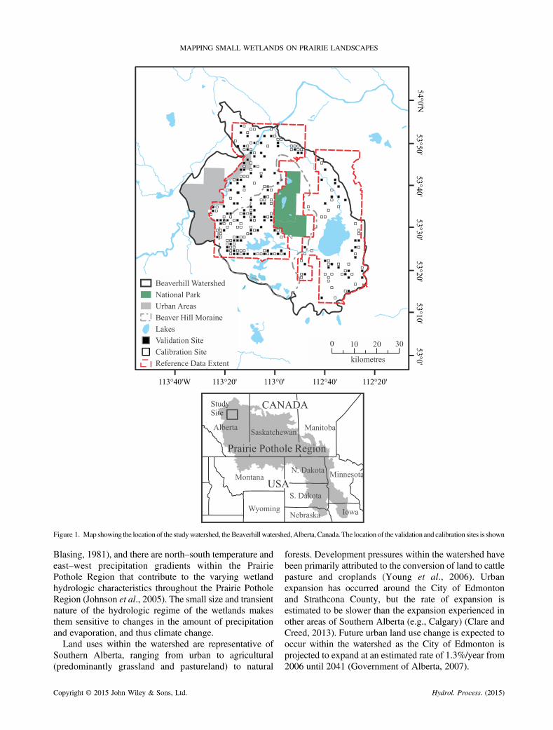
Figure 1. Map showing the location of the studywatershed, theBeaverhill watershed,Alberta, Canada. The location of the validation and calibration sites is shown

MAPPING SMALL WETLANDS ON PRAIRIE LANDSCAPES

Blasing, 1981), and there are north–south temperature andeast–west precipitation gradients within the PrairiePothole Region that contribute to the varying wetlandhydrologic characteristics throughout the Prairie PotholeRegion (Johnson et al., 2005). The small size and transientnature of the hydrologic regime of the wetlands makesthem sensitive to changes in the amount of precipitationand evaporation, and thus climate change.Land uses within the watershed are representative of

Southern Alberta, ranging from urban to agricultural(predominantly grassland and pastureland) to natural


forests. Development pressures within the watershed havebeen primarily attributed to the conversion of land to cattlepasture and croplands (Young et al., 2006). Urbanexpansion has occurred around the City of Edmontonand Strathcona County, but the rate of expansion isestimated to be slower than the expansion experienced inother areas of Southern Alberta (e.g., Calgary) (Clare andCreed, 2013). Future urban land use change is expected tooccur within the watershed as the City of Edmonton isprojected to expand at an estimated rate of 1.3%/year from2006 until 2041 (Government of Alberta, 2007).


Figure 2. TheBeaverhill Lakewater level and precipitation-potential evapotranspiration (P-PET) (growing season) for theBeaverhill watershed from1900–2010


Wetland inventory

We used multiple datasets from various sources to mapwetlands within the study area (Table I). The MMU is theminimum area of a wetland that can be reliably mappedusing a given wetland mapping method. The MMU variesfor each individual wetland mapping method and isdependent upon the resolution of the input data, any knownerrors in the data and the method used to map wetlands. Weused the high-resolution, manually delineated portion of theCWI derived from aerial photography (MMU=0.02ha) tocalibrate and validate our automatic object-based wetlandinventory derived from a light detection and ranging(LiDAR) digital elevation model (DEM). The data usedfor the manually derived wetland inventory (collected in2007) and our object-based wetland inventory (2009) werecollected within 2years of each other, and we assumed therewas no significant wetland loss from 2007–2009.

Manually delineated wetlands. Within certain areas ofthe Canadian portion of the Prairie Pothole Region, there isa high-resolution wetland inventory that was created byDucks Unlimited Canada (2014) and is part of the CWI.This manually derived high-resolution wetland inventorycovered a large portion of the study area but did not includeany urban areas. The high-resolution wetland inventorywas created from stereo-pairs derived from 1 : 20000 aerialphotographs that were captured during the growing seasonof 2007 (Figure 3). Original negatives of the images werescanned on a photogrammetric scanner to a pixel resolutionof 25 cm. Stereo-models were then created using existingground control points, and elevation data were obtained

Table I. List of data layers used in this project. Where the minimum m(MRU) was calculated by using

Data layer Resolution MRU/MM

Digital elevation model 3m MRU=0Canadian Wetland Inventory 1 : 20 000 MMU=0National Road Network 1 : 50 000 MRU=0


from a hydrologically enhanced DEM. To delineatewetland boundaries, stereo interpretation was used toidentify geomorphic and vegetative indicators of awetland’s presence, and the boundaries of the wetlandswere captured manually using this information. Individualwetland features were mapped according to the NationalWetlands Data Model (Natural Resources Canada, 2010)and classified according to the Canadian Wetland Classi-fication System (National Wetlands Working Group,1997). To meet the needs of our study, the boundaries ofthe individual wetland features were dissolved to createwetland objects. Wetlands classified as dugouts or human-made features were removed from the reference data as thefocus of this study was on natural wetlands.

Automatically delineated wetlands. A strong associa-tion exists between depressions on the landscape, definedas low-lying areas that are completely surrounded byhigher elevation, and wetland occurrence (e.g. Creedet al., 2003). A LiDAR DEM with a horizontal resolutionof 3m and an estimated vertical accuracy of 15 cm wasused to develop a probability of depression (pdep) layerthat forms the foundation of the wetland mappingtechnique. Themajority of LiDAR data were captured duringthe months of June–November of 2009 [a small amount ofLiDAR captured during the Fall (August–November) of2007 and 2008 was infilled where required] during a periodwith large moisture deficits, reducing the amount ofstanding water on the landscape.The pdep layer was developed using the Monte Carlo

method of Lindsay et al. (2004). Random elevation errors

apping unit (MMU) was not provided, a minimum resolvable unitthe method by Tobler (1987)

U (ha) Source data years Source

.0009 2009 Airborne Imaging Inc.

.02 2007 Ducks Unlimited

.25 2009 Statistics Canada


Figure 3. Flow chart showing steps used for the manually derived high-resolution portion of the reference CWI data. A, B, C and D designations indicatesteps that are comparable with those with the same letter in Figure 4, which describes the automated object-based wetland inventory using terrain objects.DEM, digital elevation model; CWI, Canadian Wetland Inventory; GPS, global positioning system; CWCS, Canadian Wetland Classification System


were added to the bare earth LiDAR DEM with a standarddeviation equal to the DEM’s vertical accuracy of 0.15m.Depressions in the DEM were filled using the Wang andLiu (2006) algorithm, and after the filling, modified cellswere identified and recorded. This process was repeateduntil a stable solution was reached, meaning that the rootmean square difference between two realizations was lessthan 0.001, with a maximum of 1000 iterations. Theprobability of depression was then calculated by thenumber of times a cell was recorded as having been filleddivided by the number of iterations. A value of 0 in thepdep layer means that the cell was not filled during any ofthe simulations and therefore has no probability of being adepression; a value of 1 indicates that the cell was filled inevery simulation and therefore has a 100% probability ofbeing a depression (Creed and Beall, 2009).The resulting pdep layer was segmented into terrain

objects following the multi-resolution segmentation algo-rithm (Baatz and Schäpe, 2000) using eCognitionDeveloper (v 8.0). By conducting object-based segmenta-tion on the probability of depression layer, we were able toimprove representation of wetland boundaries and capturea broad range of wetland size. The multi-resolutionsegmentation algorithm begins with one pixel and mergessimilar single pixels based on a pair-wise clusteringprocesses; this algorithm was conducted at different scalesto allow for the detection of both small and large wetlands(Carleer and Wolff, 2006). The pair-wise clustering


process merges regions with similar colour, smoothness,compactness to create relatively homogeneous imageobjects (Carleer and Wolff, 2006; Aldred and Wang,2011). User-specified segmentation parameters such ascolour, shape, compactness and scale can define andconstrain the segmentation process. Shape was given noweight in the segmentation in our analysis. In addition, ahigh compactness criterion (0.8) was used to producecompact terrain objects. The scale parameter in object-based segmentation is a unitless value that determines themaximum possible change in heterogeneity that can becaused by merging neighbouring image segments into onesegment (Ikokou and Smit, 2013). The lower the threshold,the lower the possible change in heterogeneity and thus thesmaller the image segment. We used a small-scaleparameter of 2 and a larger scale parameter of 20 to mapwetlands. The scale parameter of 2 is typically smaller thanwhat is used in existing wetland studies (Reif et al., 2009;Moffett and Gorelick, 2013), but it was deemed asappropriate for this study as it allowed for the detectionof small wetlands that are characteristic of prairielandscapes. The larger scale parameter was required asthe smaller scale parameter terrain objects, when classified,were found to miss portions of larger wetlands because ofthe variation in mean terrain object pdep values withinwetlands.We also buffered a vector polyline road layer for each

of the sites by 15m on each side, including the road



network line, to reduce the probability of misclassifyingroadside ditches as wetlands. Fifteen metres wasdetermined to be sufficient as the roadside ditches ofmost roads were included entirely within this buffer. This15m buffer layer was input as a vector layer to constrainthe segmentation so that the terrain objects would nottransverse roads and was also input as a binary rasterlayer that was used in the classification of terrain objects.Wetland boundaries were delineated by classifying

terrain objects. For mapping smaller wetlands (scaleparameter = 2), the mean pdep value within terrain objectsthreshold was determined using calibration sites. Weestablished 125 randomly distributed 1.5× 1.5 km cali-bration sites (Figure 1) within the watershed based on thefollowing criteria: (1) they were within the extent of thereference data in the watershed and (2) they did not have alarge water body occupying the entire site. The selectionof thresholds is important because it affects the numberand size of wetlands that are classified as wetlands. Forexample, the selection of a low mean pdep value thresholdresults in a higher number and larger size of wetlandsbeing delineated, whereas a higher mean pdep valuethreshold results in a lower number and smaller size ofwetlands.We applied nine different mean pdep thresholds to the

terrain objects at 0.05 intervals ranging from 0.30–0.70.Terrain objects with a mean pdep value greater than orequal to the nine thresholds were classified as a wetlandfor each wetland map. The Pearson coefficient (r) andabsolute difference in wetland area between the object-based wetlands and the reference wetlands were thencalculated. A threshold was selected that (1) maximizedthe r between the two images and (2) minimized theabsolute magnitude of the difference in wetland areabetween the object-based classification and the referencedata. A threshold was selected for each calibration site,and then the average threshold for all sites was calculated.For mapping larger wetlands (scale parameter = 20), thethreshold for the mean pdep value in a terrain object toclassify as a wetland was determined by iterativelyassessing smaller pdep threshold values and comparing theresults to the small scale parameter (2) results – if wetlandareas that were not being classified as wetlands using thesmaller scale parameter were classified as wetlands for agiven threshold, then the threshold was selected for thelarger scale parameter.We merged and dissolved the results of classifying

both scale parameters to form a single wetland inventory.We removed any wetland objects that had an area of lessthan the MMU of the reference data (0.02 ha) in both thereference data and the mapped data to conduct theaccuracy assessment and ensure fair comparisons. A flowchart of the method to create the manually delineatedwetlands is shown in Figure 4.


Comparison of manually derived versus automaticallyderived wetland inventories. To assess the accuracy of ourwetland mapping method, we used the segmentation andthreshold parameters that were established via the calibrationprocess on 125 validation sites that were randomlydistributed throughout the watershed. The reference dataand the object-based wetland inventories were thencompared – if a mapped wetland intersected a wetlandwithin the reference data, then that wetland was present inboth datasets and therefore assumed to be correct. Althoughthis accuracy assessment method does not compare thewetland size or shape, we deemed it to be appropriate as theshape and size of wetlands can be dynamic, varying withclimatic conditions, and therefore comparing wetland sizeand shape would likely lead to erroneous accuracy statisticsbecause the inventories were not created at the exact sametime using the exact same method and data inputs. Theomission accuracy (producer accuracy) was calculated as thenumber of wetlands in the reference data that intersect theobject-based wetland data divided by the total number ofwetlands in the reference data. The commission accuracy(user accuracy) was calculated as the number of wetlands inthe object-based mapped data that intersected the referencedata divided by the total number of wetlands in the object-based mapped data. Wetlands that did not intersect thereference data were referred to as ‘potential’wetlands due tothe fact that, without field verification, it is difficult todetermine their presence on the landscape.We also compared centroids in the reference data and the

object-based wetland inventory to further determine theaccuracy of our method. Although the shape and size ofwetlands between the two wetland inventories are likelynot similar because of the difference in time periodscaptured, the centroids of the wetlands should be close toeach other. To examine whether or not the centroids wereclose, we took all wetlands that intersected each other inthe reference data and the object-based wetland inventory.The average width of the reference wetland was thencalculated, and centroids for both data were created. Thedistance between the centroids in both data was calculatedand then compared with the average width of the referencewetland. If the distance between centroids was less than theaverage width of the reference wetland, then the mappedwetlands in both datasets were considered to be similar.

Open water permanence. We generated an open waterpermanence map by applying a different object-basedsegmentation method to historic black and white aerialphotographs and manually classifying resulting imageobjects for the years 1962, 1970, 1982, 1993, 1999 and2009. The 1962, 1993 and 2009 aerial photographs weretaken during the spring (April or May, with exception of aminor part of 1993where July andAugust 1992 imageswereused to fill in gaps and 2009 where April and May 2007


Figure 4. Flow chart of steps used for the automated object-based wetland inventory using terrain objects. See Figure 3 caption for description of A, B, Cand D designations. DTM, digital terrain model


images were used to fill in gaps). The aerial photographs for1970, 1982 and 1999 were taken in the summer of theirrespective years (July–September), except for 48% of the1982 aerial photograph, which was infilled with summer1981 data where required. This time series represents thevaryinghydrologic conditionswithin thewatershed (Figure 2).To conduct the object-based segmentation, we used a scaleparameter of 40, due to the increased spectral heterogeneitywithin the aerial photographs. We used a low shape to colourratio (0) and a compactness criterion of 0.5. We conductedoverlay analysis with inventories for the 6years, and if aportion of a wetland had water for all 6years, it wasconsidered to have 100% probability of water permanence.Both the object-based wetland inventory and the referencedata were overlaid onto the water permanence map toexamine the hydroperiod ofwetlands that were beingmapped.

Wetland loss

A power-law function of wetland area versus wetlandfrequency was used to estimate historic wetland change


(Miller et al., 2009; Zhang et al., 2009). The selection ofthe power-law function was based on the premise thatwater bodies are fractal (Brown et al., 2002), meaningthat there is a repeating pattern of water body morphom-etry at all scales, and thus, the frequency of the area ofwater bodies when plotted on logarithmic–logarithmicscales produces a straight line (negative linear relation-ship) in an undisturbed region (Kent and Wong, 1982). Adeviation from this theoretical line reflects a loss inwetland number and area if the deviation is below theline, and a gain if the deviation is above the line. Wetlandchange was estimated by the difference in area betweenthe line and the observed break in slope in the line(Figure 5). A log wetland area versus log wetlandfrequency plot was generated for wetlands larger than0.02 ha in size; the bins for wetland area were equal to theresolution of the data that was used to create the wetlandinventory [i.e. 0.0001ha (1m2)]. Piecewise linear regres-sion analyses were performed to identify breakpoints(Seber and Lee, 2012). When conducting a piecewiselinear regression, a separate regression line is fit for each


Figure 5. Interpretation of the power-law wetland area versus frequencyplots


different linear trend that occurs within the data, andbreakpoints are identified between each different trend.The breakpoint indicates an abrupt change in the data and isoften considered to be a critical threshold that can be usedfor decision-making (Vieth, 1989). First, a three-segmentpiecewise linear regression was performed; wetlandsabove the larger wetland area breakpoint were removed(the larger area breakpoint would occur at a bin with afrequency of 1, so bins with a frequency of 1 were removedfrom the analysis). Second, a two-segment piecewise linearregression was performed on the remaining data and astraight line was created by extrapolating a linearregression from the data above the smaller wetland areabreakpoint and below the larger wetland area breakpoint.Wetland number loss was calculated as the differencebetween the wetland number estimated by the theoreticalline and the actual wetland number observed for all areaclasses below the small wetland area breakpoint, andwetland area loss was calculated as the difference betweenthe wetland area estimated by the theoretical line and theactual wetland area observed for all area classes below thesmall wetland area breakpoint.

Figure 6. Probability of depression (pdep) threshold used to classify terrain obintervals were tested using 125 calibration sites. Where (a) shows the differeobject-based wetland inventory at various pdep thresholds and (b) shows the

data at various p


RESULTS

Wetland inventory technique

Calibration of technique. The statistics used to deter-mine thresholds in the mean pdep value within terrainobjects, including the correlation coefficient and theabsolute magnitude of the difference in wetland areabetween the manually and the object-based wetland data,were calculated using Whitebox [v 3]. There was a strongdownward trend with increasing pdep threshold whencalculating the absolute difference in area between thereference data and the object-based wetland inventory(Figure 6a). The trend for the correlation between the twoimages (Figure 6b) was not as clear because of the varyingresponse of each validation site to the probability ofdepression thresholds. The threshold for the small-scaleparameter of 2 was calculated to be 0.52 (any terrain objectthat had amean pdep value greater than 52%was classified asa wetland). The threshold for the larger scale parameter of20 was 0.45; when this threshold was applied to the largerterrain objects, portions of the wetland that were notcaptured by the smaller scale parameter were captured.

Validation of technique. The omission error for all of thevalidation study sites for wetlands larger than 0.02 ha insize was 18%, and the commission error was 45%. The sizeof the wetlands that were being committed or omittedwithin the validation sites (potential wetlands) tended to besmall in size (<0.5 ha), with a large number of the wetlandsbeing <0.1 ha (i.e. approximately 32×32m) (Figure 7a).Five of the validation sites were located in industrial areason the edge of the city of Edmonton. These industrialvalidation sites had higher errors, with an overall omissionerror of 21% and overall commission error of 72%.Applying object-based segmentation to the pdep maps forthe validation sites, as opposed to applying a straight pixelclassification threshold to the pdep map, decreased ourcommission error by 5%. Using object-based techniques to

jects as wetlands – potential pdep thresholds ranging from 0.3–0.7 at 0.05nce in absolute value of wetland area between the reference data and thecorrelation between the object-based wetland inventory and the referencedep thresholds


Figure 7. Frequency distribution of (a) wetland area for the validation sites within Beaverhill watershed; (b) wetlands that were mapped by the automatedobject-based method but were not contained in the reference data for the validation sites; and (c) wetlands that were not mapped by the automated object-based method but were contained in the reference data for the validation sites. In (a), black area represents those frequencies captured by the CanadianWetland Inventory (CWI) reference data and the white area represents those additional frequencies captured by the automated object-based method


segment the image into two sizes of terrain objects, wewere able to decrease the omission error by 4%. Theapplication of object-based techniques to the pdep mapsincreased the detection of wetlands on the landscape.Analysis of the distance between wetland centroids in

the reference data and the object-based wetland inventoryyielded an average distance of +6.4m between thecentroids of all intersecting wetlands. When the differencebetween the average width of the reference wetland and thedistance between the two centroids was calculated, it wasfound that 74.3% of the mapped wetlands had centroidsthat were separated by a distance that was less than theaverage width of the reference wetland, indicating a largeamount of overlap between the two wetland polygons inboth datasets.

Wetland inventory

A larger number of potential wetlands <1ha in areawere mapped than the reference data (Figure 7b, c). Withinthe validation sites, the wetland mapping techniqueidentified 5276 wetlands and potential wetlands largerthan 0.02 ha, with a total area of 2749.41 ha. The averagearea of these wetlands was 0.52 ha (range =0.02–63.33ha;median= 0.089ha), in comparison with the 1 ha averagearea of wetlands within the reference data. For the entirewatershed, 130 157 wetlands (including potential wet-lands) larger than 0.02 ha were identified, with a total areaof 111 167ha. The average wetland size for the entirewatershed was 0.85 ha (range = 0.02–19 040.19 ha;median= 0.09 ha). The object-based wetland inventorymapped 63% more wetlands and 39% more wetland areathan the reference data for the Beaverhill watershed, wherethe reference data included the manually derived wetlandinventory plus System Pour L’Observation Terre (SPOT)imagery derived wetlands for areas (about 60% of thewatershed) not covered by the manually derived wetlandinventory. The SPOT imagery was collected in 2006 and2008 and is 10m in resolution. Wetlands were mappedusing multi-spectral classification methods.We used the perimeter-to-area ratio as an indicator of the

convolutedness of the wetland boundary. The object-basedwetland inventory suggested that wetland boundaries were


more convoluted than the reference data, with the averagePA ratio being 0.22 for the object-based wetland inventory,compared with 0.15 for the CWI for wetlands greater than0.02 ha in both inventories. In addition to capturing theincreased convolution of wetland edges, the object-basedmethod was able to automatically detect hydrologicalconnections among wetlands because of the high-resolutionnature of the LiDARDEM. These hydrologically connectedwetlands appeared as individual wetlands in the referencedata; however, when an aerial photograph was underlainunder the wetland inventory, surface hydrologic connec-tions (e.g. rivers or streams) between the CWI wetlandswere observed in the aerial photographs (Figure 8). Whenthe water permanence layer was underlain on the object-based wetland inventory, it indicated that the object-basedmethod accurately detected wetlands with 100% probabilityof open water, but also detected wetlands that weretransiently filled with water. The higher number and areaof wetlands detected using the object-based method tendedto be transient wetlands (Figure 9).

Wetland loss technique

When the power-law was applied to any wetland largerthan 0.02 ha in the object-based wetland inventory, weestimated a historic loss of 16.2% number loss and 2.6%area loss (Figure 10b). The smaller wetland area breakpointfor this analysis occurred around 0.04 ha, indicating themaximum wetland area being lost was 0.04 ha.

DISCUSSION

The Prairie Pothole Region of North America containsmillions of depressional wetlands. The small and shallownature of these wetlands allows for quick conversion ofwetlands to agriculture (Galatowitsch and van der Valk,1996). To better manage these important ecosystems,improved estimates of wetland location and loss are neededto allow decision makers to balance economic anddevelopment needs while maintaining the importantfunctions and ecosystem services wetlands provide (Zedlerand Kercher, 2005).


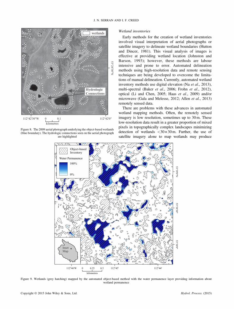
Figure 8. The 2009 aerial photograph underlying the object-based wetlands(blue boundary). The hydrologic connections seen on the aerial photograph

are highlighted

Figure 9. Wetlands (grey hatching) mapped by the automated object-basedwetland per



Wetland inventories

Early methods for the creation of wetland inventoriesinvolved visual interpretation of aerial photographs orsatellite imagery to delineate wetland boundaries (Huttonand Dincer, 1981). This visual analysis of images iseffective at providing wetland location (Johnston andBarson, 1993); however, these methods are labourintensive and prone to error. Automated delineationmethods using high-resolution data and remote sensingtechniques are being developed to overcome the limita-tions of manual delineation. Currently, automated wetlandinventory methods use digital elevation (Na et al., 2013),multi-spectral (Baker et al., 2006; Frohn et al., 2012),optical (Li and Chen, 2005; Haas et al., 2009) and/ormicrowave (Gala and Melesse, 2012; Allen et al., 2013)remotely sensed data.There are problems with these advances in automated

wetland mapping methods. Often, the remotely sensedimagery is low resolution, sometimes up to 30m. Theselow-resolution data result in a greater proportion of mixedpixels in topographically complex landscapes minimizingdetection of wetlands <30×30m. Further, the use ofsatellite imagery alone to map wetlands may produce

method with the water permanence layer providing information aboutmanence


Figure 10. Interpretation of the power-law applied to any wetland objectgreater than 0.02 ha in the object-based wetland inventory. Historically,there has been an estimated 16.17% number loss and 2.56% area loss of

wetlands


inaccurate results because of spectral similarities betweendifferent types of vegetation (Ozesmi and Bauer, 2002;Maxa and Bolstad, 2009). The accuracy of theseautomated wetland-mapping techniques improves whenancillary data are considered. For example, Maxa andBolstad (2009) used high-resolution LiDAR data andIKONOS imagery to map wetlands. They manuallycaptured wetland boundaries using a fusion of the twoimages and found that using a combination of LiDAR andIKONOS was 18.5% more accurate than the WisconsinWetland Inventory maps for the same region (Maxa andBolstad, 2009). Lang et al. (2012) developed topographicindices from a LiDAR DEM and compared them withexisting inundation and wetland maps. They found that ahybrid of topographic indices (e.g. topographic wetnessindices and relief information) provided a good indicationof wetland location and inundation period and that theresulting maps using the hybrid topographic indicatorswere similar to existing aerial photograph-derived wetlandmaps. These studies indicate that topographic information,such as those derived from LiDAR DEMs, can assist inmapping wetlands.The automated wetland mapping technique developed

in this study, based on terrain objects derived fromLIDAR DEMs, was effective at mapping wetlands andsensitive to capturing small (<1ha) wetlands that arecharacteristic of the Prairie Pothole Region. A highernumber and area of small, ephemeral wetlands that wereon the landscape but not included in the reference datawere detected based on the water permanence map. UsingLiDAR data to map wetlands is particularly advantageousin the prairies because LiDAR can effectively delineatewetlands in areas with low relief and detect smalldepressions (Lindsay et al., 2004; Lindsay and Creed,2005; Lang et al., 2010). Additionally, as shown by theincreased perimeter-to-area ratio in our automated


wetland inventory in comparison with the reference data,the object-based techniques were able to better capture thehydrologically dynamic wetland boundaries. The object-based segmentation and classification of LiDAR datacontributed to the success of our method because itconsiders terrain homogeneity within not only the object,but also the surrounding pixels as well as the spatiallocation of the terrain object (Moffett and Gorelick,2013). The automated approach to developing wetlandinventories will allow managers to monitor changes in thespatial and temporal distribution of wetlands and todevelop policies to reduce the vulnerability of thesewetlands to further loss.Another advantage of our wetland mapping method is

that it is time independent when compared with otherwetland mapping methods. When using aerial photogra-phy or other satellite imagery to map wetlands, it is oftendifficult to delineate the full extent of the individualwetland basin as the vegetation patterns may makeestablishing the boundary of the wetland difficult incertain types of wetlands (e.g. ephemeral wetlands), andwetland boundaries are extremely dynamic and dependenton the climate of a given year (Maxa and Bolstad, 2009).Further, it is dependent on the time of year and the seasonthe remotely sensed images were collected in. To mapwetlands using aerial photographs or satellite imagery,visual cues, pixel values or spectral signatures arerequired, which are affected by the time and date of yearthey are captured. One advantage of creating a wetlandmapping method based on LiDAR data is that the resultsare less sensitive to climate and time of year to the samedegree as aerial photographs and satellite images.However, to achieve the best results, LiDAR should becaptured in the driest part of the year, or during dry years,to capture the full extent of any depressions because it isless able to penetrate the surface of the water.A potential drawback of our automatic wetland

mapping method is that it is sensitive to land use.Specifically, it is effective at detecting the presence ofwetlands in natural and agricultural land types; however,it is less effective in urban and industrialized areas. It isunable to distinguish between natural and man-madedepressions on the landscape; e.g. in urban and industrialareas, the wetland mapping method detects man-madefeatures such as the depressions surrounding industrialtanks that are then included in the wetland inventory.Therefore, as indicated by the high commission errors inindustrial areas of the watershed, the application of ourmethod to urban areas should be carried out cautiously.To conduct our wetland mapping method in other

geographic regions, segmentation parameters and meanterrain object pdep thresholds will require modification.We have provided the necessary tools within theSupporting Information (including the software used for



calculating pdep as well as the segmentation rule sets foreCognition Developer) for this wetland mapping methodto be modified and used by wetland managers.

Wetland loss

The power-law function is based on the negative linearrelationship that exists between wetland area and frequen-cy when plotted on log–log scales. A deviation from thistheoretical line indicates either wetland loss or gain. Thebenefits of using the power-law to estimate wetland loss arethat only a wetland inventory is required for input into thepower-law, and it provides a standardized method forassessing wetland loss rate estimates. However, to detectthe break in slope, high-resolution wetland inventories arerequired as deviations from the theoretical relationshiptypically occur at wetland size classes that are <0.5 ha insize. A portion of the deviation from the theoretical linecould be attributed to a landscape that has increaseddrainage or evapotranspiration that affects wetland char-acteristics such as soils, plants and water. This can make itdifficult to differentiate wetlands from surroundinguplands. However, our wetland inventory was not createdbased on the spectral properties of soils, plants and water,but the presence of a depression that holds water, at leasttemporarily. Depressions can be detected under differingclimate conditions and are sensitive to climate; thus, weassume that our deviation is due to wetland loss.The power-law is sensitive to the selection of the area

class size (i.e. the interval of wetland area on the x-axis ofthe power-law plot), the wetland area minimum andmaximum thresholds to be included in the analysis andminimum frequency within the area class size bins used togenerate the plot. Increasing the area class size results in anincrease in both % area and % number loss because of theincrease in frequency in the area classes that break from thetheoretical line. Having the area class equal to the pixel sizeof the input data used to create the wetland inventoryallows for more accurate wetland area loss estimates as awetland within the inventory can only increase in area bythe size of the pixel. To our knowledge, there are noexisting studies that test the effects of modifying thepower-law parameters. Previous studies have used thepower-law to assess the difference in wetland distributionon the landscape over time (e.g. Van Meter and Basu,2014), but the power-law has not been used to directlyestimate the magnitude of wetland loss. In addition to thearea class size, the power-law is also sensitive to thenumber of wetlands within a wetland inventory. Theapproach should not be used for small geographic areas(<500km2) with a small sample size of wetlands (<10 000wetlands) because there may not be a high enoughfrequency in the area classes to form a useable power-law. For this reason, it is recommended that this analysis becarried out at a regional watershed scale at a minimum.


The accuracy of our estimated wetland loss can becompared with other estimates within the region.Environment Canada estimated wetland loss in theCanadian prairies by estimating wetland loss along aseries of transects. Watmough (2011) estimated cumulativewetland loss by combining recent lost area (1985–2011) andhistoric (drained or filled wetland basins mapped at the timeof the 1985 baseline) estimates, with a minimum mappingunit for the field campaign ranging from 0.015–0.022ha.They used aerial photograph analyses and field verificationto delineate wetlands and identify any sign of anthropogenicdisturbances. This approach to monitoring wetland losses istime consuming and requires data that typically do not existat high enough resolution over large geographic areas, andtherefore cannot be used to obtain estimates of wetland lossacross the entire Canadian prairies. The results of their studycalculated a mean cumulative historic wetland area lossranging from 1.6–53.2% per transection in the Beaverhillwatershed region. Our area estimate of 2.6% is towards thelower end of the range of loss estimates. Watmough andSchmoll (2007) also found that the average size of lostwetlands was 0.20ha, supporting our observation of thepreferential loss of small wetlands within the prairies.Several studies cite wetland loss rates for the developedareas of Canada (e.g. Bedford, 1999; Warner and Asada,2006; Austen and Hanson, 2007). Our power-law analysisfound a much lower wetland area loss within the Beaverhillwatershed, a phenomenon that could be attributed to thelarge part of the Beaverhill watershed that is designated asparks or protected areas.

Future research needs

Future work using the power-law will focus onapplying the method to the entire Prairie Pothole Regionto provide a geographically based assessment of wetlandloss (e.g., where is the highest historic wetland loss?) andapplying the method to a time series of wetlandinventories to determine the rate of wetland loss overtime. This will allow us to look at wetland change in thecontext of wetland policies that have been implementedand allow us to examine the effectiveness of policyactions to arrest wetland loss over time.

CONCLUSION

This study demonstrates how the ability of wetlandinventory mapping methods to detect small wetlands andcapture edge boundary convolutedness can be improvedby the use of LiDAR DEMs and object-based techniques.With the increasing availability of LiDAR data, thiswetland mapping method shows promise for mappingwetlands over large geographic regions. These wetlandinventories will be able to provide information on the



location of individual wetlands and the density anddistribution of wetlands over landscapes, providinginsight into the ability of a wetland to provide functionsand ecosystem services. Further, the application a power-law function to the wetland inventory provides a simple,standardized method to estimate historic wetland lossrates. The wetland mapping and loss estimation methodsdeveloped here have the ability to improve wetlandmanagement and wetland policies.

ACKNOWLEDGEMENTS

This research was supported by an Alberta WetlandResearch Initiative Grant and a National Science andEngineering Research Council (NSERC) of CanadaDiscovery Grant to I. F.C. and a NSERC CGS-M awardto J.N. S. We acknowledge David Aldred for his technicalassistance with the development of the mapping tech-nique. We also acknowledge Lyle Boychuk of DucksUnlimited Canada for providing the reference data andDr Michael Watmough of Environment Canada forproviding wetland loss data.

REFERENCES

Aldred DA, Wang J. 2011. A method for obtaining and applyingclassification parameters in object-based urban rooftop extraction fromVHR multispectral images. International Journal of Remote Sensing32: 2811–2823.

Allen R, Wang T, Gore B. 2013. Coastal wetland mapping combiningmulti-date SAR and LiDAR. Geocarto International 28: 616–631.

Austen E, Hanson A. 2007. An analysis of wetland policy in AtlanticCanada. Canadian Water Resources Journal 32: 163–178.DOI:10.4296/cwrj3203163.

Baatz M, Schäpe A. 2000. Multi-resolution segmentation: an optimizationapproach for high quality multi-scale image segmentation. Paperpresented at the Applied Geographical Data Processing SymposiumXII Heidelberg, Germany.

Badiou P, McDougal R, Pennock D, Clark B. 2011. Greenhouse gasemissions and carbon sequestration potential in restored wetlands of theCanadian prairie pothole region. Wetlands Ecology and Management19: 237–256. DOI:10.1007/s11273-011-9214-6.

Baker C, Lawrence R, Montagne C, Patten D. 2006. Mapping wetlandsand riparian areas using Landsat ETM+ imagery and decision-tree-based models. Wetlands 26: 465–474. DOI:10.1672/0277-5212(2006)26[465:MWARAU]2.0.CO;2.

Bedford BL. 1999. Cumulative effects on wetland landscapes: links towetland restoration in the United States and southern Canada. Wetlands19: 775–788. DOI:10.1007/BF03161784.

Brown JH, Gupta VK, Li BL, Milne BT, Restrepo C, West GB. 2002. Thefractal nature of nature: power-laws, ecological complexity andbiodiversity. Philosophical Transactions of the Royal Society, B:Biological Sciences 357: 619–626. DOI:10.1098/rstb.2001.0993.

Carleer AP, Wolff E. 2006. Urban land cover multi-level region-basedclassification ofVHRdata by selecting relevant features. International Journalof Remote Sensing 27: 1035–1051. DOI:10.1080/01431160500297956.

Clare S, Creed IF. 2013. Tracking wetland loss to improve evidence-basedwetland policy learning and decision making. Wetlands Ecology andManagement 22: 235–245. DOI:10.1007/s11273-013-9326-2.

Craft CB, Casey WP. 2000. Sediment and nutrient accumulation infloodplain and depressional freshwater wetlands of Georgia, USA.Wetlands 20: 323–332. DOI:10.1672/0277-5212(2000)020[0323:SANAIF]2.0.CO;2.


Creed IF, Beall FD. 2009. Distributed topographic indicators forpredicting nitrogen export from headwater catchments. Water Re-sources Research 45: . DOI:10.1029/2008WR007285.

Creed IF, Sanford SE, Beall FD, Molot LA, Dillon PJ. 2003. Crypticwetlands: integrating hidden wetlands in regression models of theexport of dissolved organic carbon from forested landscapes. Hydro-logical Processes 17: 3629–3648. DOI:10.1002/hyp.1357.

Creed IF, Miller J, Aldred D, Adams JK, Spitale S, Bourbonniere RA.2013. Hydrologic profiling for greenhouse gas effluxes from naturalgrasslands in the prairie pothole region of Canada. Journal ofGeophysical Research, Biogeosciences 118: 680–697. DOI:10.1002/jgrg.20050.

Crumpton WG, Goldsborough LG. 1998. Nitrogen transformation and fatein prairie wetlands. Great Plains Research 8: .

Dahl TE. 2014. Status and Trends of Prairie Wetlands of the United States1997 to 2009. U.S. Department of the Interior, Fish and WildlifeService, Ecological Services: Washington D.C..

Dahl TE, Watmough MD. 2007. Current approaches to wetland status andtrends monitoring in prairie Canada and the continental United States ofAmerica. Canadian Journal of Remote Sensing 33: S17–S27.DOI:10.5589/m07-050.

Davidson NC. 2014. How much wetland has the world lost? Long-termand recent trends in global wetland area. Marine and FreshwaterResearch 65: 934–941. DOI: doi.org/10.1071/MF14173.

Ducks Unlimited Canada. 2014. Canadian wetland inventory [data file].Retrieved from Ducks Unlimited Canada.

Dunne EJ, Smith J, Perkins DB, Clark MW, Jawitz JW, Reddy KR. 2007.Phosphorus storages in historically isolated wetland ecosystems andsurrounding pasture uplands. Ecological Engineering 31: 16–28.DOI:10.1016/j.ecoleng.2007.05.004.

Duvick D, Blasing T. 1981. A dendroclimatic reconstruction of annualprecipitation amounts in Iowa since 1680. Water Resources Research17: 1183–1189. DOI:10.1029/WR017i004p01183.

Environment Canada. 2010. Canadian climate normals. Retrieved onjanuary 5, 2014 from http://climate.weather.gc.ca/climate_normals/index_e.html.

Finlayson CM, Davidson NC, Spiers AG, Stevenson NJ. 1999. Globalwetland inventory–current status and future priorities. Marine andFreshwater Research 50: 717–727. DOI:10.1071/MF99098.

Fournier RA, Grenier M, Lavoie A, Hélie R. 2007. Towards a strategy toimplement the Canadian Wetland Inventory using satellite remotesensing. Canadian Journal of Remote Sensing 33: S1–S16.DOI:10.5589/m07-051.

Frohn RC, D’Amico E, Lane C, Autrey B, Rhodus J, Liu H. 2012. Multi-temporal sub-pixel Landsat ETM+ classification of isolated wetlands inCuyahoga County, Ohio, USA. Wetlands 32: 289–299. DOI:10.1007/s13157-011-0254-8.

Gala T, Melesse A. 2012. Monitoring prairie wet area with an integratedLANDSAT ETM+, RADARSAT-1 SAR and ancillary data fromLIDAR. Catena 95: 12–23. DOI:10.1016/j.catena.2012.02.022.

Galatowitsch S, van der Valk A. 1996. Vegetation and environmentalconditions in recently restored wetlands in the prairie pothole region ofthe USA. Vegetatio 126: 89–99. DOI:10.1007/BF00047764.

Government of Alberta. 2007. Working together: report of the capitalregion integrated growth management plan project team. Edmonton,Alberta 1–111.

Haas E, Bartholomé E, Combal B. 2009. Time series analysis of opticalremote sensing data for the mapping of temporary surface water bodiesin sub-Saharan western Africa. Journal of Hydrology 370: 52–63.DOI:10.1016/j.jhydrol.2009.02.052.

Hamon WR. 1961. Estimating potential evapotranspiration. Proceedingsof the American Society of Civil Engineers Journal of HydraulicDivision 87: 107–120.

Howitt RW. 1988. Soil survey of the County of Beaver (Vol. 47): Albertasoil survey report.

Hutton SM, Dincer T. 1981. Using Landsat imagery to study theOkavango Swamp, Botswana. Paper presented at the Proceedings of theFifth Annual William T. Pecora Memorial Symposium on RemoteSensing, Sioux Falls, South Dakota

Ikokou GB, Smit J. 2013. A technique for optimal selection ofsegmentation scale parameters for object-oriented classification ofurban scenes. South African Journal of Geomatics 2: 358–369.


http://climate.weather.gc.ca/climate_normals/index_e.html

http://climate.weather.gc.ca/climate_normals/index_e.html


Johnson WC, Millett BV, Gilmanov T, Voldseth R, Guntenspergen G,Naugle D. 2005. Vulnerability of northern prairie wetlands to climatechange. BioScience 55: 863–872. DOI:10.1641/0006-3568(2005)055[0863:VONPWT]2.0.C.

Johnston C. 2013. Wetland losses due to row crop expansion in theDakota Prairie Pothole Region. Wetlands 33: 175–182. DOI:10.1007/s13157-012-0365-x.

Johnston RM, Barson MM. 1993. Remote sensing of Australian wetlands:an evaluation of Landsat TMdata for inventory and classification.Marineand Freshwater Research 44: 235–252. DOI:10.1071/MF9930235.

Kantrud HA, Krapu GL, Swanson GA, Allen JA. 1989. Prairie basinwetlands of the Dakotas: a community profile: DTIC document

Kent C, Wong J. 1982. An index of littoral zone complexity and itsmeasurement. Canadian Journal of Fisheries and Aquatic Sciences 39:847–853. DOI:10.1139/f82-115.

Lane C, D’Amico E. 2010. Calculating the ecosystem service of waterstorage in isolated wetlands using LiDAR in North Central Florida,USA. Wetlands 30: 967–977. DOI:10.1007/s13157-010-0085-z.

Lane C, Autrey B, Jicha T, Lehto L, Elonen C, Seifert-Monson L. 2015.Denitrification potential in geographically isolated wetlands of NorthCarolina andFlorida,USA.Wetlands1–13.DOI:10.1007/s13157-015-0633-7.

Lang M, McCarty G, Wilen B, Awl J. 2010. Light detection and ranging:new information for improved wetland mapping and monitoring.National Wetlands Newsletter 32: 10–13.

Lang M, McCarty G, Oesterling R, Yeo I. 2012. Topographic metrics forimproved mapping of forested wetlands. Wetlands 33: 141–155.DOI:10.1007/s13157-012-0359-8.

Li J, Chen W. 2005. A rule-based method for mapping Canada’s wetlandsusing optical, radar and DEM data. International Journal of RemoteSensing 26: 5051–5069. DOI:10.1080/01431160500166516.

Lindsay JB, Creed IF. 2005. Sensitivity of digital landscapes to artifactdepressions in remotely-sensed DEMs. Photogrammetric Engineeringand Remote Sensing 71: 1029–1036.

Lindsay JB, Creed IF, Beall FD. 2004. Drainage basin morphometrics fordepressional landscapes. Water Resources Research 40: . DOI:10.1029/2004WR003322.

Martin GI, Kirkman LK, Hepinstall-Cymerman J. 2012. Mappinggeographically isolated wetlands in the Dougherty Plain, Georgia,USA. Wetlands 32: 149–160. DOI:10.1007/s13157-011-0263-7.

Marton JM, Creed IF, Lewis DB, Lane CR, Basu NB, Cohen MJ, CraftCB. 2015. Geographically isolated wetlands are important biogeo-chemical reactors on the landscape. BioScience 65: 408–418.DOI:10.1093/biosci/biv009.

Maxa M, Bolstad P. 2009. Mapping northern wetlands with highresolution satellite images and LiDAR. Wetlands 29: 248–260.DOI:10.1672/08-91.1.

McLaughlin DL, Kaplan DA, Cohen MJ. 2014. A significant nexus:geographically isolated wetlands influence landscape hydrology. WaterResources Research 50: 7153–7166. DOI:10.1002/2013WR015002.

Miller BA, Crumpton WG, van der Valk AG. 2009. Spatial distribution ofhistoric wetland classes on the Des Moines Lobe, Iowa. Wetlands 29:1146–1152. DOI:10.1672/08-158.1.

Moffett KB, Gorelick SM. 2013. Distinguishing wetland vegetation andchannel features with object-based image segmentation. InternationalJournal of Remote Sensing 34: 1332–1354. DOI:10.1080/01431161.2012.718463.

Na X, Zang S, Liu L, Li M. 2013. Wetland mapping in the ZhalongNational Natural Reserve, China, using optical and radar imagery andtopographical data. Journal of Applied Remote Sensing 7: .DOI:10.1117/1.JRS.7.073554.

National Wetlands Working Group. 1997. In the Canadian WetlandClassification System, Warner B, Rubec C (eds). Wetlands ResearchBranch, University of Waterloo: Waterloo, Ontario.

NaturalRegions Committee. 2006.Natural regions and subregions of Alberta.Compiled by DJ Downing, WW Pettapiece. Government of Alberta.

Natural Resources Canada. 2010. National wetlands data model:Geomatics Canada.

Naugle DE, Johnson RR, Estey ME, Higgins KF. 2001. A landscapeapproach to conserving wetland bird habitat in the prairie pothole region


of eastern South Dakota. Wetlands 21: 1–17. DOI:10.1672/0277-5212(2000)020[0588:ALATCW]2.0.CO;2.

Ozesmi SL, Bauer ME. 2002. Satellite remote sensing of wetlands.Wetlands Ecology and Management 10: 381–402. DOI:10.1023/A:1020908432489.

Pomeroy JW, Shook K, Fang X, Dumanski S, Westbrook C, Brown T.2014. Improving and Testing the Prairie Hydrological Model at SmithCreek Research Basin. University of Saskatchewan: Centre forHydrology: Saskatoon, Saskatchewan; 1–102.

Reddy K, Kadlec R, Flaig E, Gale P. 1999. Phosphorus retention instreams and wetlands: a review. Critical Reviews in EnvironmentalScience and Technology 29: 83–146. DOI:10.1080/10643389991259182.

Reif M, Frohn R, Lane C, Autrey B. 2009. Mapping isolated wetlands in akarst landscape: GIS and remote sensing methods. GIScience & RemoteSensing 46: 187–211. DOI:10.2747/1548-1603.46.2.187.

Seber GA, Lee AJ. 2012. Linear Regression Analysis. John Wiley & Sons:Hoboken, New Jersey; 936.

Semlitsch RD, Bodie JR. 1998. Are small, isolated wetlands expendable?Conservation Biology 12: 1129–1133. DOI:10.1046/j.1523-1739.1998.98166.x.

Tiner RW. 2003. Geographically isolated wetlands of the United States.Wetlands 23: 494–516. DOI:10.1672/0277-5212(2003)023[0494:GIWOTU]2.0.CO;2.

Tobler W. 1987. Measuring spatial resolution. Paper presented at theInternational Workshop on Geographical Information Systems, Beijing.

van der Valk AG, Pederson RL. 2003. The SWANCC decision and itsimplications for prairie potholes. Wetlands 23: 590–596. DOI:10.1672/0277-5212(2003)023[0590:TSDAII]2.0.CO;2.

Van Meter KJ, Basu NB. 2014. Signatures of human impact: sizedistributions and spatial organization of wetlands in the prairie potholelandscape. Ecological Applications . DOI:10.1890/14-0662.1.

Vieth E. 1989. Fitting piecewise linear regression functions to biologicalresponses. Journal of Applied Physiology 67: 390–396.

Wang L, Liu H. 2006. An efficient method for identifying and fillingsurface depressions in digital elevation models for hydrologic analysisand modelling. International Journal of Geographical InformationScience 20: 193–213. DOI:10.1080/13658810500433453.

Warner BG, Asada T. 2006. Knowledge gaps and challenges in wetlandsunder climate change in Canada. In Climate Change and ManagedEcosystems, Lal R, Price M, Apps M, Bhatti J (eds). CRC Press:Boca Raton, Florida; 355–372.

Watmough MD. 2011. Gross wetland loss estimates [dataset].Watmough MD, Schmoll MJ. 2007. Environment Canada’s Prairie andNorthern Region Habitat Monitoring Program Phase II: RecentHabitat Trends in the Prairie Habitat Joint Venture. EnvironmentCanada, Canadian Wildlife Service: Edmonton, Alberta, Canada.

Westbrook CJ, Brunet N, Phillips I, Davies J-M. 2011. Wetland drainageeffects on prairie water quality – final report. Centre for HydrologyReport No. 9.

Young JE, Sánchez-Azofeifa GA, Hannon SJ, Chapman R. 2006. Trendsin land cover change and isolation of protected areas at the interface ofthe southern boreal mixedwood and aspen parkland in Alberta, Canada.Forest Ecology and Management 230: 151–161. DOI:10.1016/j.foreco.2006.04.031.

Zedler JB, Kercher S. 2005. Wetland resources: status, trends, ecosystemservices, and restorability. Annual Review of Environment andResources 30: 39–74. DOI:10.1146/annurev.energy.30.050504.144248.

Zhang B, Schwartz FW, Liu G. 2009. Systematics in the size structure ofprairie pothole lakes through drought and deluge. Water ResourcesResearch 45: DOI:10.1029/2008WR006878.

SUPPORTING INFORMATION

Additional supporting information may be found in theonline version of this article at the publisher’s web-site.


Documents

New mapping techniques to estimate the preferential loss