New High Performing Heuristics for Minimizing Makespan … · New High Performing Heuristics for Minimizing Makespan in Permutation Flowshops ... 2 The Nawaz, Enscore and Ham

New High Performing Heuristics for Minimizing

Makespan in Permutation Flowshops

Shahriar Farahmand Rad1, Rubén Ruiz2∗, Naser Boroojerdian1

1 Faculty of Mathematics and Computer Sciences, Amirkabir University of Technology,

Tehran, Iran. {farahmand,broojerd}@aut.ac.ir

2 Dept. of Applied Statistics and Operations Research, Polytechnic University of Valencia,

Valencia, Spain. [email protected]

May 25, 2006

Abstract

The well known NEH heuristic from Nawaz, Enscore and Ham proposed in 1983 has

been recognized as the highest performing method for the permutation flowshop schedul-

ing problem under the makespan minimization criterion. This performance lead is main-

tained even today when compared against contemporary and more complex heuristics as

shown in recent studies. In this paper we show five new methods that outperform NEH

as supported by careful statistical analyses using the well known instances of Taillard.

The proposed methods try to counter the excessive greediness of NEH by carrying out

re-insertions of already inserted jobs at some points in the construction of the solution.

The five proposed heuristics range from extensions that are slightly slower than NEH in

most tested instances to more comprehensive methods based on local search that yield

excellent results at the expense of some added computational time. Additionally, NEH

has been profusely used in the flowshop scheduling literature as a seed sequence in high

performing metaheuristics. We demonstrate that using some of our proposed heuristics

as seeds yields better final results in comparison.

Keywords: scheduling, flowshop, makespan, heuristics

∗Corresponding author. Tel: +34 96 387 70 07, ext: 74946. Fax: +34 96 387 74 99

1

1 Introduction

Flowshop scheduling deals about determining the best sequence of n jobs that are to be processed

on m machines in the same order. pij denotes the non-negative, known and deterministic processing

time of job j at machine i. Without loss of generality, we can assume that all jobs visit machine 1

first, then machine 2 and so on until machine m. It is common in the scheduling literature to look

for a sequence of jobs that minimizes the maximum completion time which coincides with the time

at which the last job in the sequence finishes at machine m. This objective is commonly referred to

as makespan or Cmax.

There are a number of assumptions that are usually considered (Baker, 1974):

• All jobs are independent and available for processing at time 0.

• Machines are continuously available.

• At any time, each machine can process at most one job and each job can be processed only

on one machine.

• The processing of a given job at a machine cannot be interrupted, i.e, no preemption is allowed.

• Setup times are sequence independent and are included in the processing times or otherwise

can be ignored.

• An infinite in-process storage buffer is assumed. If a given job needs an unavailable machine

then it joins a queue of unlimited size waiting for that machine.

Generally, there are as many possible sequences as there are job permutations and since this permu-

tations can change from machine to machine, the solution space contains (n!)m schedules. However,

in the flowshop scheduling literature this general case is seldom considered. A common simplification

is to have the same permutation for all machines. Hence n! schedules are possible and the problem

is denoted as F/prmu/Cmax following the notation given in Graham et al. (1979). This problem is

also known as the permutation flowshop scheduling problem or PFSP in short.

The PFSP with only two machines (m = 2) was shown in 1954 to be polynomially solvable to opti-

mality in O(n log n) steps by Johnson. However, for three or more machines, the problem is known

to be NP-Complete in the strong sense (Garey et al., 1976).

The PFSP has been thoroughly studied in the literature and there are literally hundreds of pa-

pers published that deal with flowshops or similar problems. Focusing on the PFSP with Cmax, some

of the classical and most cited heuristics were proposed by Page (1961), Palmer (1965), Campbell

et al. (1970), Gupta (1971), Aggarwal and Stafford (1975), Bonney and Gundry (1976), Dannenbring

(1977), King and Spachis (1980) and Stinson and Smith (1982). All these methods are previous to

the NEH algorithm of Nawaz et al. (1983). After this date, many papers in which newer algo-

rithms were proposed have been published. Some examples are Hundal and Rajgopal (1988), Ho

2

and Chang (1991), Sarin and Lefoka (1993), Koulamas (1998), Suliman (2000) and Davoud Pour

(2001), to name just a few. These methods and many other less known heuristics are excellently

reviewed in Framinan et al. (2004). A complete computational evaluation of methods is provided in

Ruiz and Maroto (2005) and another recent review is given by Hejazi and Saghafian (2005).

Several studies place NEH as the best performing method. Direct evaluations against older

methods are given in Turner and Booth (1987) and Taillard (1990) where NEH is shown to provide

better results than other highly cited heuristics such as the CDS method of Campbell et al. (1970).

More importantly, in Ruiz and Maroto (2005), NEH was tested against 25 other heuristics, including

the more modern and complex algorithms of Koulamas (1998), Suliman (2000) and Davoud Pour

(2001), as well as those of Hundal and Rajgopal (1988) and Ho and Chang (1991). The results,

supported by careful statistical analyses, show that NEH is vastly superior to all tested methods

and at the same time much faster. As a result, NEH is used today as a seed sequence in many, if

not all, effective metaheuristics proposed for the PFSP. Some examples where the NEH is used as

a seed sequence for Tabu Search, Simulated Annealing, Genetic Algorithms, Iterated Local Search,

Ant Colony Optimization and many other metaheuristic algorithms can be seen in Reeves (1993),

Chen et al. (1995), Reeves (1995), Murata et al. (1996), Nowicki and Smutnicki (1996), Reeves and

Yamada (1998), Stützle (1998), Wang and Zheng (2003), Rajendran and Ziegler (2004), Grabowski

and Wodecki (2004), Ruiz et al. (2006) and Ruiz and Stützle (2006). This is just a small extract of

the many algorithms that rely on NEH for an effective initialization.

In this paper we study several alternative algorithms that make use of the principles of the NEH

heuristic and try to overcome some of its drawbacks. We propose five new heuristics that range

from key extensions that provide significantly better results at a slightly CPU time penalty to more

comprehensive improvements based on local search that yield excellent results at the expense of some

added computational time. We carry out large experimentations and careful statistical analyses to

soundly test the results. Additionally, and given the large body of literature that makes use of NEH

as an initialization, we test the effect of using some of the proposed methods as a seed sequence in

contrast to NEH. The statistically significant results indicate that using our proposed methods as

seed sequences provides better results in many recent state-of-the-art metaheuristics.

The remainder of this paper is organized as follows: Section 2 provides a comprehensive intro-

duction to the NEH heuristic. Section 3 provides the explanations of the five new proposed heuristics

which are later comprehensively evaluated in Section 4. In Section 5 we study the benefits of using

the new proposed methods as seed sequences in some of the best existing metaheuristics. Finally,

the conclusions of this study are given in Section 6.

3

2 The Nawaz, Enscore and Ham (NEH) heuristic

The NEH procedure is based on the idea that jobs with high processing times on all the machines

should be scheduled as early as possible. NEH is divided into three simple steps:

1. Calculate the total processing times of all jobs:

Pj =m

∑

i=1

pij

2. Jobs are sorted in descending order of Pj .

3. Take job j, j = 1, . . . , n and find the best schedule by placing it in all the possible j positions

in the sequence of jobs that are already scheduled. For example, if j = 3, the already built

sequence would contain the first two jobs of the sorted list calculated in step 2, then, the third

job could be placed either in the first, in the second, or in the third position of the sequence.

The best sequence of the three would be selected for the next iteration in which the fourth

job will be considered.

Given a sequence π of n jobs, where π(j) denotes the job in the jth position, the makespan (Cmax)

of a given sequence can be calculated with the following formulae:

Ci,π(j)= max

{

Ci−1,π(j), Ci,π(j−1)

}

+ piπ(j)

Cmax = Cm,π(n)(1)

where Ci,j denotes the completion time of job j at machine i. Additionally, C0,π(j)= 0 and Ci,π(0)

= 0,

∀i ∈ M, ∀j ∈ N . Calculating the Cmax has a complexity of O(nm).

As can be seen, step 1 has a complexity of O(nm). Second step is just an ordering and takes

O(n log n). In step 3 we have a loop of n steps where at each step j we carry out j insertions of jobs

and for each insertion we have to calculate the Cmax value of j jobs. In total, there are n(n+1)2 − 1

insertions (when j = 1 there are no insertions to be made). Only in the last step we have the

complete n jobs so the complexity is O(n3m) which can be slow, specially for larger values of n. A

closer look at the previous formulae shows that when inserting the jth job in position, let’s say, k, all

Ci,h, h = {k − 1, k − 2, . . . , 1} were already calculated in the previous insertion. A similar approach

was followed by Taillard (1990) and as a result the complexity of all insertions in a given step can be

calculated in O(nm) by a series of matrix calculations. This reduces the total complexity of NEH

to O(n2m). Such improved method is many times referred to as NEHT or NEH with Taillard’s

accelerations. As it will be shown in later sections, NEHT is extremely fast even for large values of

n.

Some authors have studied the NEH method, but mainly the first and second steps. Framinan et al.

(2003) studied 177 different initial orders for the jobs prior to start insertions at step 3. While this

4

study was carried out for different objectives, as regards Cmax, the order initially proposed by Nawaz

et al. (1983) was shown to be the most effective. Ruiz et al. (2006) used a modified version of NEH

in which after step 2, some jobs were exchanged at random. This resulted in a NEH method that can

be used for generating different good individuals for the initial population in Genetic Algorithms.

One possible criticism of the NEH method is that once a job is inserted into the sequence, the

relative position with respect to the other existing jobs is not changed as the algorithm progresses.

When inserting a new job, many times it is beneficial to reconsider previously inserted jobs in order

to better accommodate this new job. Another possible drawback is that NEH is essentially a greedy

method. At each step we look for the best possible place for the job while possibly a not so best

position will result in better solutions once the next job in the sequence is inserted. Our proposed

heuristics try to take advantage of these drawbacks in order to improve the results.

3 New heuristics

In this section we propose five new high performing heuristics. The first two are based on some well

known mathematic properties of the PFSP problem and the later three use the idea of re-inserting

already scheduled jobs.

Let M = (pij), 1 ≤ i ≤ m, 1 ≤ j ≤ n, be the matrix of processing times in the PFSP. It is known in

the scheduling literature that the following directed graph can be constructed where the nodes are

weighted with the processing times:

p11• −→

p12• −→

p13• −→ · · · −→

p1,m−1• −→

p1m

•

↓ ↓ ↓ ↓ ↓p21• −→

p22• −→

p23• −→ · · · −→

p2,m−1• −→

p2m

•

↓ ↓ ↓ ↓ ↓p31• −→

p32• −→

p33• −→ · · · −→

p3,m−1• −→

p3m

•

↓ ↓ ↓ ↓ ↓...

......

......

↓ ↓ ↓ ↓ ↓pn1• −→

pn2• −→

pn3• −→ · · · −→

pn,m−1• −→

pnm

•

As shown in Bellman et al. (1982) the makespan of a flow shop problem is equal to the length of the

longest path between vertices (1, 1) and (n, m) in the corresponding directed graph obtained from

the matrix M . Columns in this matrix cannot be swapped or exchanged since they represent the

different machines but in order to reduce the length of the longest path in the graph we can arrange

the rows (jobs) accordingly. Therefore, the PFSP problem can be seen as an arrangement of rows

in M so that the length of the longest path is reduced. As it is shown in Figure 1, arrows in the

constructed directed graph are such that if the a given solution passes through (i, j) then it is not

5

possible to reach node (i′, j′), if i < i′, j′ < j or if i′ < i, j < j′.

[Insert Figure 1 about here]

Additionally, and as shown in Figure 2, if the line which is drawn between two possible nodes has a

positive slope, then it is not possible to reach one path from the other.


Based on this idea, we choose the rows in M one by one and evaluate the possible nodes at each row

while trying to minimize Cmax. This method is somehow similar to NEH method. The fundamental

difference is that in the NEH, rows are selected according to Pj whereas in the first two proposed

algorithms, selection of jobs is based on the weights of the different nodes ofthe same row. This

means that each row is selected a maximum of m times. Following the above discussion, we present

the first algorithm, referred to as FRB1, in Figure 3.


As it can be seen, we first sort in decreasing order all processing times pij in a vector called PV .

We start with an empty processing time matrix M ′ that will be filled as the algorithm progresses.

Then we carry out n · m steps. At each step we take the next element in PV which corresponds to

the processing time of a given job and machine. We copy this processing time in M ′ and extract

the job if it was already in the solution. Then we insert the job (if new) or re-insert it in all possible

positions of the incumbent sequence. The new position for the job is the one that results in the

lowest Cmax. Notice that the processing times matrix M ′ is not complete until the last step.

It can be seen that we have n · m steps and at each step the most expensive calculation is the

calculation of the Cmax values for all possible positions of the job. The worst case is when all n jobs

are already in the solution and this can be done in O(nm) steps using Taillard’s accelerations as in

the NEHT method. Therefore, the complexity of the FRB1 algorithm is O(n2m2).

The second algorithm, called FRB2, is a simple modification of FRB1 in which we do not use

the matrix M ′ and rather consider always all processing times. The pseudocode of the algorithm is

shown in Figure 4.


It should be noted that if at a given step, the job selected is the same as the job that was selected in

the previous step, we do nothing and skip to the next step (being all the processing times present,

there is no point in re-inserting the job in all possible positions since the outcome is not going to

change). Therefore, although the computational complexity of FRB2 is the same as that of FRB1,

the empirical running time is expected to be slightly lower.

The three remaining methods are based in a different principle. After inserting one new job into

6

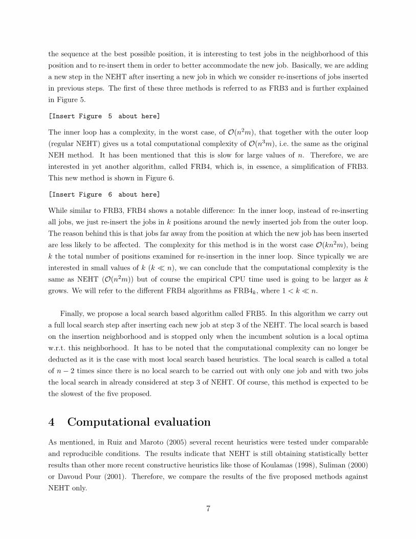
the sequence at the best possible position, it is interesting to test jobs in the neighborhood of this

position and to re-insert them in order to better accommodate the new job. Basically, we are adding

a new step in the NEHT after inserting a new job in which we consider re-insertions of jobs inserted

in previous steps. The first of these three methods is referred to as FRB3 and is further explained

in Figure 5.


The inner loop has a complexity, in the worst case, of O(n2m), that together with the outer loop

(regular NEHT) gives us a total computational complexity of O(n3m), i.e. the same as the original

NEH method. It has been mentioned that this is slow for large values of n. Therefore, we are

interested in yet another algorithm, called FRB4, which is, in essence, a simplification of FRB3.

This new method is shown in Figure 6.


While similar to FRB3, FRB4 shows a notable difference: In the inner loop, instead of re-inserting

all jobs, we just re-insert the jobs in k positions around the newly inserted job from the outer loop.

The reason behind this is that jobs far away from the position at which the new job has been inserted

are less likely to be affected. The complexity for this method is in the worst case O(kn2m), being

k the total number of positions examined for re-insertion in the inner loop. Since typically we are

interested in small values of k (k ≪ n), we can conclude that the computational complexity is the

same as NEHT (O(n2m)) but of course the empirical CPU time used is going to be larger as k

grows. We will refer to the different FRB4 algorithms as FRB4k, where 1 < k ≪ n.

Finally, we propose a local search based algorithm called FRB5. In this algorithm we carry out

a full local search step after inserting each new job at step 3 of the NEHT. The local search is based

on the insertion neighborhood and is stopped only when the incumbent solution is a local optima

w.r.t. this neighborhood. It has to be noted that the computational complexity can no longer be

deducted as it is the case with most local search based heuristics. The local search is called a total

of n − 2 times since there is no local search to be carried out with only one job and with two jobs

the local search in already considered at step 3 of NEHT. Of course, this method is expected to be

the slowest of the five proposed.

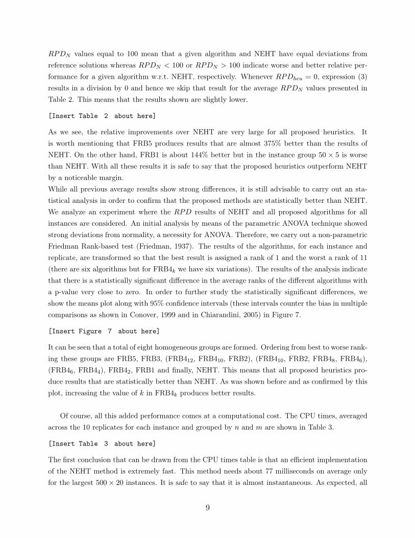
4 Computational evaluation

As mentioned, in Ruiz and Maroto (2005) several recent heuristics were tested under comparable

and reproducible conditions. The results indicate that NEHT is still obtaining statistically better

results than other more recent constructive heuristics like those of Koulamas (1998), Suliman (2000)

or Davoud Pour (2001). Therefore, we compare the results of the five proposed methods against

NEHT only.

7

We implement NEHT and FRB1-FRB5 heuristics in Delphi 2006 and carry out all tests on a Pentium

IV PC/AT computer running at 3.2 GHz with 2 GBytes of RAM memory. All algorithms share most

code and especially the critical functions that evaluate the Cmax as well as Taillard’s accelerations.

Therefore, results are completely comparable.

For the comparisons we use the well known, standard benchmark set of Taillard (1993). This set

comprises 120 instances divided into 12 groups with 10 replicates each. The sizes range from 20

jobs, 5 machines to 500 jobs, 20 machines. Authors in the flowshop scheduling literature have been

using this benchmark extensively in the past years. For each instance, a very tight lower bound and

upper bound is known. At the time of the writing of this paper, all 10 instances in the 50 × 20 set,

nine in 100 × 20, six in 200 × 20 and three in 500 × 20 are still open. For all other instances, the

optimum solution is already known.

Taking this into account, the performance measure that we will be using is the Relative Percentage

Deviation (RPD) over the optimum or best known solution (upper bound) for each instance:

Relative Percentage Deviation (RPD) =Heusol − Bestsol

Bestsol

× 100 (2)

where Heusol is the solution given by any of the tested heuristics for a given instance and Bestsol

is the optimum solution or the lowest known upper bound for Taillard’s instances as of May 2006.

These best solutions are available at Taillard (2006). It has to be noted that FRB5 is a local search

based algorithm and therefore it is stochastic in nature. In order to better estimate its performance,

a total of 10 replicates for each instance are carried out and the results averaged. All other algo-

rithms are deterministic but we also carry out 10 replicates so to better estimate the elapsed CPU

time. Finally, for heuristic FRB4k we test k = {2, 4, 6, 8, 10, 12}. The results for all methods are

shown in Table 1.

[Insert Table 1 about here]

The average results indicate that all proposed algorithms outperform NEHT. Only on some excep-

tions NEHT provides better results. More specifically, NEHT outperforms FRB1 in 30 cases, gives

better solutions in 2 cases and worse in 88 instances. For FRB2 this three values (better NEHT,

equal to NEHT and worse NEHT) are 12, 3 and 105. For FRB3 these values are 3, 2 and 115 whereas

for FRB42 and FRB412 21, 4, 95 and 3, 3, 114, respectively. Finally, for FRB5, NEHT gives better

solution only in 2 cases, equal solution in 3 cases and worse solution in all 115 remaining instances.

So it is clear than the proposed methods outperform the classical NEHT method. Another way of

looking at the results of Table 1 is to transform the data so that we see the Relative Percentage

Deviation over the NEHT method (RPDN ):

Relative Percentage Deviation over NEHT (RPDN ) =RPDNEHT

RPDheu

× 100 (3)

8

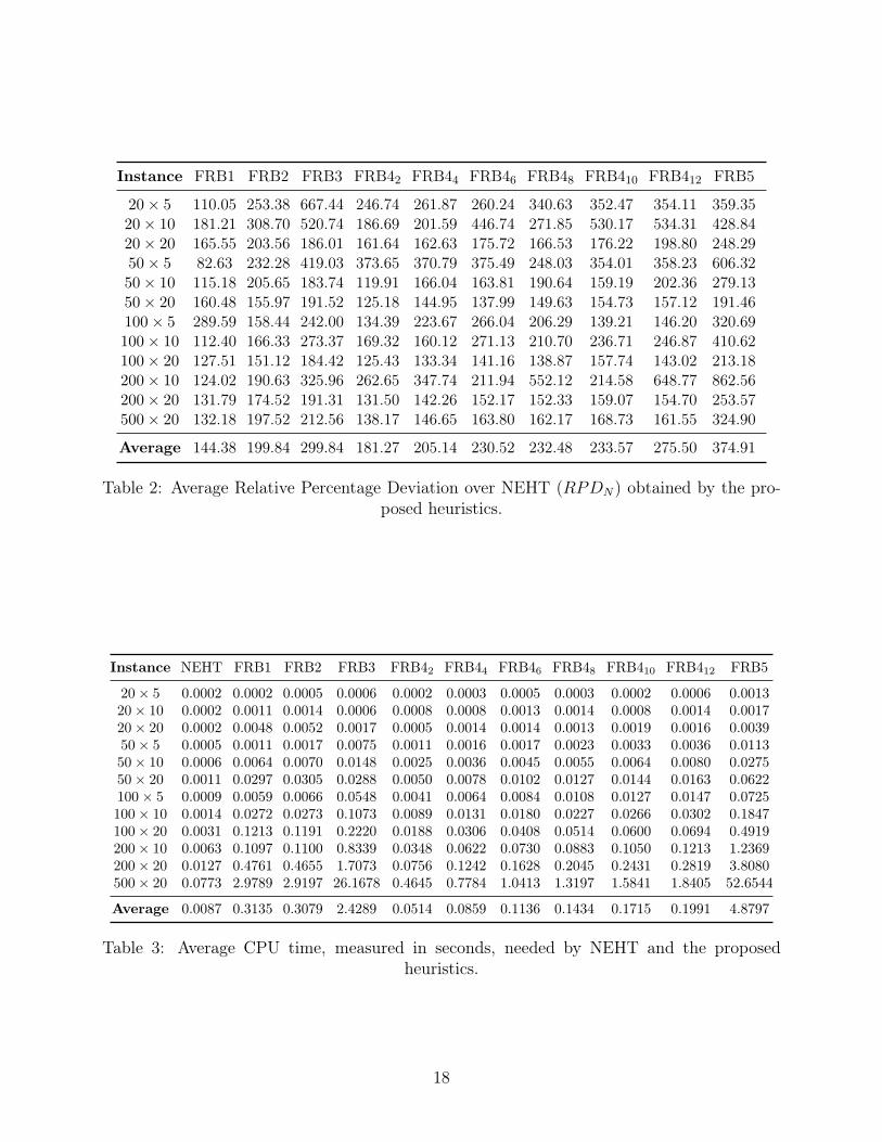
RPDN values equal to 100 mean that a given algorithm and NEHT have equal deviations from

reference solutions whereas RPDN < 100 or RPDN > 100 indicate worse and better relative per-

formance for a given algorithm w.r.t. NEHT, respectively. Whenever RPDheu = 0, expression (3)

results in a division by 0 and hence we skip that result for the average RPDN values presented in

Table 2. This means that the results shown are slightly lower.


As we see, the relative improvements over NEHT are very large for all proposed heuristics. It

is worth mentioning that FRB5 produces results that are almost 375% better than the results of

NEHT. On the other hand, FRB1 is about 144% better but in the instance group 50 × 5 is worse

than NEHT. With all these results it is safe to say that the proposed heuristics outperform NEHT

by a noticeable margin.

While all previous average results show strong differences, it is still advisable to carry out an sta-

tistical analysis in order to confirm that the proposed methods are statistically better than NEHT.

We analyze an experiment where the RPD results of NEHT and all proposed algorithms for all

instances are considered. An initial analysis by means of the parametric ANOVA technique showed

strong deviations from normality, a necessity for ANOVA. Therefore, we carry out a non-parametric

Friedman Rank-based test (Friedman, 1937). The results of the algorithms, for each instance and

replicate, are transformed so that the best result is assigned a rank of 1 and the worst a rank of 11

(there are six algorithms but for FRB4k we have six variations). The results of the analysis indicate

that there is a statistically significant difference in the average ranks of the different algorithms with

a p-value very close to zero. In order to further study the statistically significant differences, we

show the means plot along with 95% confidence intervals (these intervals counter the bias in multiple

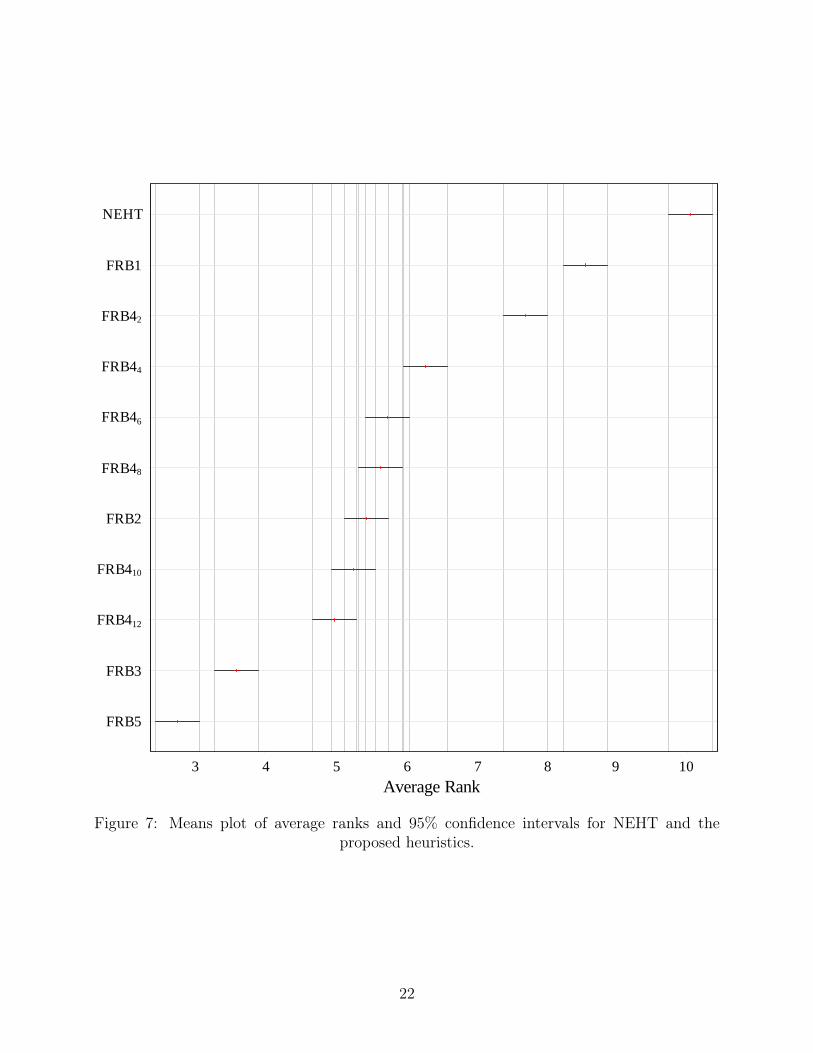
comparisons as shown in Conover, 1999 and in Chiarandini, 2005) in Figure 7.


It can be seen that a total of eight homogeneous groups are formed. Ordering from best to worse rank-

ing these groups are FRB5, FRB3, (FRB412, FRB410, FRB2), (FRB410, FRB2, FRB48, FRB46),

(FRB46, FRB44), FRB42, FRB1 and finally, NEHT. This means that all proposed heuristics pro-

duce results that are statistically better than NEHT. As was shown before and as confirmed by this

plot, increasing the value of k in FRB4k produces better results.

Of course, all this added performance comes at a computational cost. The CPU times, averaged

across the 10 replicates for each instance and grouped by n and m are shown in Table 3.


The first conclusion that can be drawn from the CPU times table is that an efficient implementation

of the NEHT method is extremely fast. This method needs about 77 milliseconds on average only

for the largest 500 × 20 instances. It is safe to say that it is almost instantaneous. As expected, all

9

other methods are slower but it has to be stressed that they are still very fast. Among the proposed

heuristics, the fastest is FRB42 which needs 51 milliseconds on average and less than half a second

for the largest instances. Considering that this heuristic is about 181% better than NEHT, such

an increase of CPU time seems justified. Increasing the value of k has detrimental effects on CPU

time as could be expected. In any case, increasing k all the way to 12 as in FRB412 results in CPU

times of about 0.2 seconds on average and less than 2 seconds for the largest instances which can

be still considered as a very fast heuristic. Recall that FRB412 is about 375% better than NEHT.

The methods motivated by the directed graph concept, namely FRB1 and FRB2, are also very fast

with about a third of a second on average. Only for the largest instances these methods need times

measured in less than three seconds. Finally, FRB3, which re-inserts all previously inserted jobs in

a given step and FRB5, which is based on local search, are significantly slower as one could expect.

Nevertheless, both methods have large CPU time needs only for the 500 × 20 instances and very

reasonable CPU times for the other instances. For example, FRB3 is, on average, 521% better than

NEHT on the 20 × 10 set and it only needs about 0.6 milliseconds (on the verge of our ability to

measure CPU time). Another example is FRB5 which is a whooping 863% better than NEHT in

the 200 × 10 set needing 1.2 seconds. From our perspective, such an increase of CPU time is easily

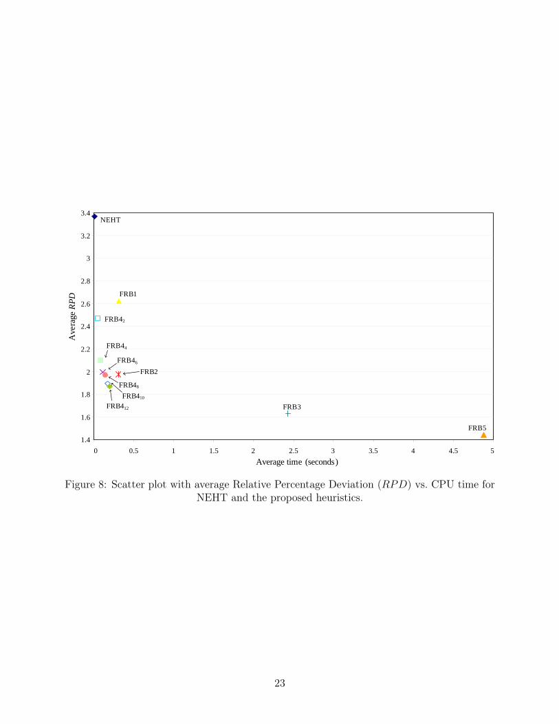
justified in view of the quality of results obtained. Finally, the scatter plot shown in Figure 8 depicts

the average RPD versus average CPU times for all methods.


As shown, even though NEHT is staggeringly fast, most proposed methods provide much better

results under half a second on average.

5 Using the proposed heuristics as seed sequences

In this Section we now answer to the question of what improvements can be expected if our proposed

methods are used as seed sequences for more elaborated and costlier metaheuristics. In order to

do so, we use three recent, high performing metaheuristics and a classical method. We test the

Simulated Annealing of Osman and Potts (1989), refereed to as SA_OP. This method originally

starts from a random solution and here we test initializations with several of our proposed meth-

ods. Additionally, we test the best Ant Colony Optimization algorithm of Rajendran and Ziegler

(2004), which we will refer to as PACO. This method uses NEHT as an initialization. We also test

the hybrid Genetic Algorithm of Ruiz et al. (2006) (HGA_RMA) which initializes the population

by using NEHT. Lastly, we test the recent Iterated Greedy method with local search of Ruiz and

Stützle (2006) (IG_RSLS). This simple algorithm was shown to yield state-of-the-art results for the

permutation flowshop problem with Cmax criterion.

We carry out a careful experimental design. We control three main factors. The main one is the

10

algorithm itself which has four levels (SA_OP, PACO, HGA_RMA and IG_RSLS). The second

factor is the type of initialization which also takes four levels (Default, FRB2, FRB3 and FRB5).

The last factor is the type of instance which is a discrete factor with 12 levels, one for 20× 5 and so

on until 12 for 500× 20. Note that n and m cannot be considered as separated factors since not all

combinations exist in Taillard’s benchmark instances. For each combination of factors we run the

algorithms 10 times with each Taillard’s instance so there is a grand total of 4 · 4 · 10 · 120 = 19, 200

treatments.

All algorithms share the same stopping criterion, which is elapsed CPU time. This time is set to

a value that depends on the size of the instance to n · (m/2) · 30 milliseconds. All algorithms are

carefully coded so that they use exactly this time in order to avoid deviations in the results. This

elapsed time allows for 1.5 seconds in the smallest 20 × 5 instances and 150 seconds for the largest

500 × 20 set. This time is large enough to observe if an effective initialization still improves the

results of a given algorithm. Obviously, with a sufficiently large time, all algorithms are expected to

obtain good results regardless of the initialization.

In the resulting experiment, all three factors as well as all two-factor interactions are clearly

significant with p-values very close to zero. The type of algorithm is the most significant factor

(highest F-Ratio), meaning that the four tested metaheuristics show, as expected, different perfor-

mance. For some “easy” instances, namely those with small n and m, the effect of the initialization is

very difficult to observe, i.e. more or less all algorithms are capable of obtaining very good solutions

(many times optimal) regardless of the heuristic used for obtaining the seed sequence. However,

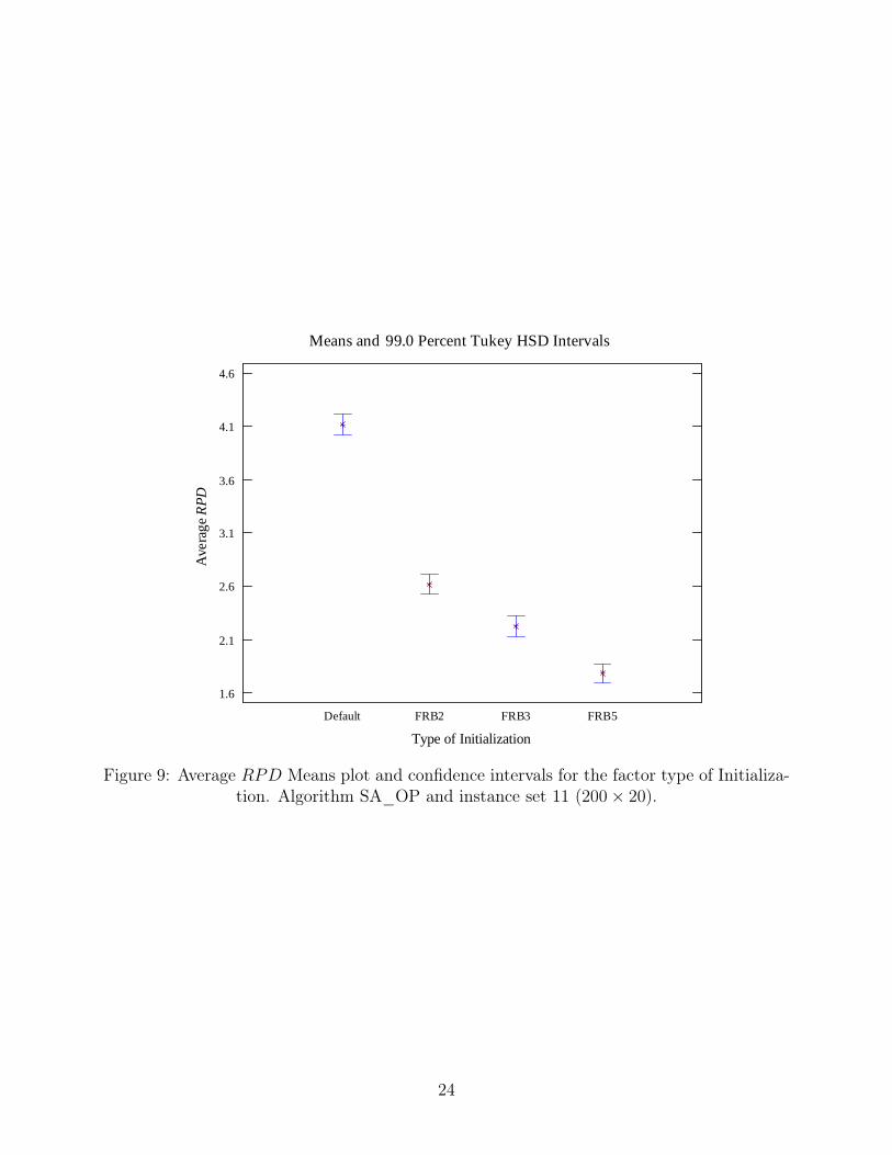
for some algorithms and not so easy instances, the initialization makes a big difference. Figure 9

shows the means plot for the initialization factor after having fixed the algorithm to SA_OP and

the instance set 11 (200 × 20).


As it can be seen, SA_OP benefits greatly from a better initialization. Similarly, for the tested

proposed algorithms, FRB2, FRB3 and FRB5, solutions improve steadily, obtaining the best statis-

tically significant results with FRB5. Note that we are using Honest Significant Difference (HSD)

intervals which counteract the bias in multiple pairwise comparisons and we are also considering a

high level of confidence (99%). Recall that non-overlapping intervals mean that the observed means

are statistically different. The picture is more or less similar for other algorithms if one focuses on

the hard to solve instances. However, since default for other algorithms is indeed NEHT, we see less

differences between this default initialization and FRB2, for example.

Another question is if for the largest instances for which we have 150 seconds, the costlier FRB3 and

FRB5 heuristics provide any advantage over NEHT. Figure 10 depicts the means plot for algorithm

PACO and instance set 12 (500 × 20).


11

Here we see that FRB2 is statistically not preferred to NEHT and this last one is equivalent to

FRB3. However, results are vastly improved when FRB5 (which consumes about a third of the time

PACO has available) is used for initialization. Similar results are obtained for other algorithms as

shown in Figure 11 for IG_RSRS .


In this case NEHT, FRB2 and FRB3 provide statistically similar results but once again FRB5 pro-

vides statistically better results and by a noticeably margin. Notice that the Y-axis indicates the

average RPD obtained for the 10 instances in the 500× 20 set and 10 replicates (i.e., 100 results for

each means plotted). The average result given by the FRB5 initialization is 0.52 versus the average

given by the default of 0.6. This means an improvement of about 15%. We hypothesize that it is

very “expensive” for the tested metaheuristic algorithms to reach a high-quality solution in a limited

time starting from a worse solution. High performing heuristics are complementary to these sort of

metaheuristic methods. The latter are capable to continue the search once the heuristic has finished

and to do a more in-depth, finely-tuned search from that point. Starting from random or low quality

solutions implies that the metaheuristic method has to work a long way in order to reach promising

regions of the search space.

Although not shown here, short experiments with a lower CPU time stopping criterion, like for

example n · (m/2) · 15 milliseconds, resulted in even more pronounced differences for all methods

while times over n · (m/2) · 100 ms. or more neglected most statistically significant differences. As a

result, we can conclude that the tested classical SA_OP algorithm as well a current state-of-the-art

methods such as PACO, HGA_RMA and IG_RSLS benefit from a good seed solution given by the

proposed methods.

6 Conclusions

In this paper we have shown five new high performing constructive heuristics for the well known

permutation flowshop scheduling problem under the minimization of the makespan or Cmax. It is

well known that the NEH heuristic of Nawaz et al. (1983) is the best constructive heuristic for this

problem according to several studies (Turner and Booth (1987), Taillard (1990) and Ruiz and Maroto

(2005)), being significantly better than other more recent approaches. One of the key strengths of the

NEH is that it performs insertions of jobs while constructing the sequence, which is in itself a type

of a very direct local search. However, the insertion is carried out in a greedy fashion which results,

in some cases, in solutions far from optimum values. Our proposed heuristics try to counteract this

excessive greediness by re-inserting previously inserted jobs. We have conducted a comprehensive

set of computational experiments and statistical analyses that demonstrate that the five proposed

heuristics outperform in most cases the NEH heuristic, and in some cases by almost 863%. For some

12

of the proposed methods, the CPU time penalty is very small as most heuristics yield solutions in

less than half a second on average.

Additionally, we have tested the effect of initializing several state-of-the-art existing metaheuristics

with some of our proposed methods in contrast to an initialization with the NEH method. Namely, we

have tested an Iterated Greedy method, a hybrid Genetic Algorithm, an Ant Colony Optimization

procedure as well as a classical Simulated Annealing algorithm. The statistically sound results

indicate that using even our most CPU demanding heuristic yields significant improvements when

used as a seed sequence in the tested methods.

As a conclusion, our proposed heuristics can be regarded as the new best fast constructive heuristics

for the permutation flowshop scheduling problem with makespan objective.

Acknowledgments

Rubén Ruiz is partly funded by the Spanish Department of Science and Technology (research project

ref. DPI2004-06366-C03-01).

References

Aggarwal, S. C. and Stafford, Jr, E. F. (1975). A heuristic algorithm for the flowshop problem with

a common sequence on all machines. Decision Sciences, 6(2):237–251.

Baker, K. R. (1974). Introduction to Sequencing and Scheduling. John Wiley & Sons, New York.

Bellman, R., Esogbue, A. O., and Nabeshima, I. (1982). Mathematical Aspects of Scheduling and

Applications. Pergamon Press, New York.

Bonney, M. and Gundry, S. (1976). Solutions to the constrained flowshop sequencing problem.

Operational Research Quarterly, 27(4):869–883.

Campbell, H. G., Dudek, R. A., and Smith, M. L. (1970). A heuristic algorithm for the n job, m

machine sequencing problem. Management Science, 16(10):B630–B637.

Chen, C.-L., Vempati, V. S., and Aljaber, N. (1995). An application of genetic algorithms for flow

shop problems. European Journal of Operational Research, 80:389–396.

Chiarandini, M. (2005). Stochastic local search methods for highly constrained combinatorial optimi-

sation problems. PhD thesis, Computer Science Department. Darmstadt University of Technology.

Darmstadt, Germany.

Conover, W. (1999). Practical Nonparametric Statistics. John Wiley & Sons, New York, third

edition.

13

Dannenbring, D. G. (1977). An evaluation of flow shop sequencing heuristics. Management Science,

23(11):1174–1182.

Davoud Pour, H. (2001). A new heuristic for the n-job, m-machine flow-shop problem. Production

Planning and Control, 12(7):648–653.

Framinan, J. M., Gupta, J. N. D., and Leisten, R. (2004). A review and classification of heuristics for

permutation flow-shop scheduling with makespan objective. Journal of the Operational Research

Society, 55:1243–1255.

Framinan, J. M., Leisten, R., and Rajendran, C. (2003). Different initial sequences for the heuristic

of Nawaz, Enscore and Ham to minimize makespan, idletime or flowtime in the static permutation

flowshop sequencing problem. International Journal of Production Research, 41(1):121–148.

Friedman, M. (1937). The use of ranks to avoid the assumption of normality implicit in the analysis

of variance. Journal of the American Statistical Association, 32:675–701.

Garey, M. R., Johnson, D. S., and Sethi, R. (1976). The complexity of flowshop and jobshop

scheduling. Mathematics of Operations Research, 1(2):117–129.

Grabowski, J. and Wodecki, M. (2004). A very fast tabu search algorithm for the permutation glow

shop problem with makespan criterion. Computers & Operations Research, 31:1891–1909.

Graham, R. L., Lawler, E. L., Lenstra, J. K., and Rinnooy Kan, A. H. G. (1979). Optimization

and approximation in deterministic sequencing and scheduling: A survey. Annals of Discrete

Mathematics, 5:287–326.

Gupta, J. N. D. (1971). A functional heuristic algorithm for the flowshop scheduling problem.

Operational Research Quarterly, 22(1):39–47.

Hejazi, S. R. and Saghafian, S. (2005). Flowshop-scheduling problems with makespan criterion: a

review. International Journal of Production Research, 43(14):2895–2929.

Ho, J. C. and Chang, Y.-L. (1991). A new heuristic for the n-job, m-machine flow-shop problem.

European Journal of Operational Research, 52:194–202.

Hundal, T. S. and Rajgopal, J. (1988). An extension of Palmer’s heuristic for the flow shop scheduling

problem. International Journal of Production Research, 26(6):1119–1124.

Johnson, S. M. (1954). Optimal two- and three-stage production schedules with setup times included.

Naval Research Logistics Quarterly, 1:61–68.

King, J. R. and Spachis, A. S. (1980). Heuristics for flow-shop scheduling. International Journal of

Production Research, 18(3):345–357.

14

Koulamas, C. (1998). A new constructive heuristic for the flowshop scheduling problem. European

Journal of Operational Research, 105:66–71.

Murata, T., Ishibuchi, H., and Tanaka, H. (1996). Genetic algorithms for flowshop scheduling

problems. Computers & Industrial Engineering, 30(4):1061–1071.

Nawaz, M., Enscore, Jr, E. E., and Ham, I. (1983). A heuristic algorithm for the m-machine, n-

job flow-shop sequencing problem. OMEGA, The International Journal of Management Science,

11(1):91–95.

Nowicki, E. and Smutnicki, C. (1996). A fast tabu search algorithm for the permutation flow-shop

problem. European Journal of Operational Research, 91:160–175.

Osman, I. and Potts, C. (1989). Simulated annealing for permutation flow-shop scheduling. OMEGA,

The International Journal of Management Science, 17(6):551–557.

Page, E. S. (1961). An approach to the scheduling of jobs on machines. Journal of the Royal

Statistical Society, B Series, 23(2):484–492.

Palmer, D. S. (1965). Sequencing jobs through a multi-stage process in the minimum total time - a

quick method of obtaining a near optimum. Operational Research Quarterly, 16(1):101–107.

Rajendran, C. and Ziegler, H. (2004). Ant-colony algorithms for permutation flowshop scheduling to

minimize makespan/total flowtime of jobs. European Journal of Operational Research, 155:426–

438.

Reeves, C. and Yamada, T. (1998). Genetic algorithms, path relinking, and the flowshop sequencing

problem. Evolutionary Computation, 6(1):45–60.

Reeves, C. R. (1993). Improving the efficiency of tabu search for machine scheduling problems.

Journal of the Operational Research Society, 44(4):375–382.

Reeves, C. R. (1995). A genetic algorithm for flowshop sequencing. Computers & Operations

Research, 22(1):5–13.

Ruiz, R. and Maroto, C. (2005). A comprehensive review and evaluation of permutation flowshop

heuristics. European Journal of Operational Research, 165:479–494.

Ruiz, R., Maroto, C., and Alcaraz, J. (2006). Two new robust genetic algorithms for the flowshop

scheduling problem. OMEGA, the International Journal of Management Science, 34:461–476.

Ruiz, R. and Stützle, T. (2006). A simple and effective iterated greedy algorithm for the permutation

flowshop scheduling problem. European Journal of Operational Research. In press.

15

Sarin, S. and Lefoka, M. (1993). Scheduling heuristic for the n-job m-machine flow shop. OMEGA,

The International Journal of Management Science, 21(2):229–234.

Stinson, J. P. and Smith, A. W. (1982). A heuristic programming procedure for sequencing the

static flowshop. International Journal of Production Research, 20(6):753–764.

Stützle, T. (1998). Applying iterated local search to the permutation flow shop problem. Technical

report, AIDA-98-04, FG Intellektik,TU Darmstadt.

Suliman, S. M. A. (2000). A two-phase heuristic approach to the permutation flow-shop scheduling

problem. International Journal of Production Economics, 64:143–152.

Taillard, E. (1990). Some efficient heuristic methods for the flow shop sequencing problem. European

Journal of Operational Research, 47:67–74.

Taillard, E. (1993). Benchmarks for basic scheduling problems. European Journal of Operational

Research, 64:278–285.

Taillard, E. (2006). Summary of best known lower and upper bounds of Taillard’s

instances. http://ina.eivd.ch/collaborateurs/etd/problemes.dir/ordonnancement.dir/

ordonnancement.html.

Turner, S. and Booth, D. (1987). Comparison of heuristics for flow shop sequencing. OMEGA, The

International Journal of Management Science, 15(1):75–78.

Wang, L. and Zheng, D. Z. (2003). An effective hybrid heuristic for flow shop scheduling. The

International Journal of Advanced Manufacturing Technology, 21:38–44.

16

Instance NEHT FRB1 FRB2 FRB3 FRB42 FRB44 FRB46 FRB48 FRB410 FRB412 FRB5

20 × 5 3.35 3.57 1.52 0.89 2.02 1.22 1.24 1.14 1.11 1.12 1.0820 × 10 5.02 3.11 2.54 1.86 3.23 2.70 2.20 2.45 1.80 1.79 2.1920 × 20 3.73 2.34 2.17 2.18 2.49 2.40 2.24 2.26 2.18 2.08 1.80

50 × 5 0.84 0.91 0.40 0.22 0.32 0.40 0.29 0.43 0.34 0.30 0.19

50 × 10 5.12 4.44 3.10 2.99 4.32 3.11 3.31 2.79 3.45 2.89 2.25

50 × 20 6.31 4.19 4.11 3.36 5.08 4.39 4.59 4.30 4.14 4.04 3.37100 × 5 0.46 0.42 0.30 0.21 0.39 0.18 0.18 0.32 0.25 0.28 0.16

100 × 10 2.13 1.92 1.34 0.94 1.58 1.38 1.04 1.12 1.17 1.22 0.80

100 × 20 5.23 4.16 3.52 2.90 4.31 4.00 3.74 3.80 3.39 3.73 2.51

200 × 10 1.43 1.22 0.89 0.52 0.75 0.67 0.71 0.61 0.73 0.60 0.38

200 × 20 4.52 3.46 2.62 2.41 3.49 3.22 2.99 2.99 2.84 2.95 1.84

500 × 20 2.24 1.68 1.16 1.06 1.62 1.52 1.39 1.40 1.33 1.40 0.72

Average 3.37 2.62 1.97 1.63 2.47 2.10 1.99 1.97 1.89 1.87 1.44

Table 1: Average Relative Percentage Deviation (RPD) over the optimum or best knownsolution obtained by NEHT and the proposed heuristics. Italics and bold figures indicate

worst and best values, respectively.

17

Instance FRB1 FRB2 FRB3 FRB42 FRB44 FRB46 FRB48 FRB410 FRB412 FRB5

20 × 5 110.05 253.38 667.44 246.74 261.87 260.24 340.63 352.47 354.11 359.3520 × 10 181.21 308.70 520.74 186.69 201.59 446.74 271.85 530.17 534.31 428.8420 × 20 165.55 203.56 186.01 161.64 162.63 175.72 166.53 176.22 198.80 248.2950 × 5 82.63 232.28 419.03 373.65 370.79 375.49 248.03 354.01 358.23 606.3250 × 10 115.18 205.65 183.74 119.91 166.04 163.81 190.64 159.19 202.36 279.1350 × 20 160.48 155.97 191.52 125.18 144.95 137.99 149.63 154.73 157.12 191.46100 × 5 289.59 158.44 242.00 134.39 223.67 266.04 206.29 139.21 146.20 320.69100 × 10 112.40 166.33 273.37 169.32 160.12 271.13 210.70 236.71 246.87 410.62100 × 20 127.51 151.12 184.42 125.43 133.34 141.16 138.87 157.74 143.02 213.18200 × 10 124.02 190.63 325.96 262.65 347.74 211.94 552.12 214.58 648.77 862.56200 × 20 131.79 174.52 191.31 131.50 142.26 152.17 152.33 159.07 154.70 253.57500 × 20 132.18 197.52 212.56 138.17 146.65 163.80 162.17 168.73 161.55 324.90

Average 144.38 199.84 299.84 181.27 205.14 230.52 232.48 233.57 275.50 374.91

Table 2: Average Relative Percentage Deviation over NEHT (RPDN) obtained by the pro-posed heuristics.

Instance NEHT FRB1 FRB2 FRB3 FRB42 FRB44 FRB46 FRB48 FRB410 FRB412 FRB5

20 × 5 0.0002 0.0002 0.0005 0.0006 0.0002 0.0003 0.0005 0.0003 0.0002 0.0006 0.001320 × 10 0.0002 0.0011 0.0014 0.0006 0.0008 0.0008 0.0013 0.0014 0.0008 0.0014 0.001720 × 20 0.0002 0.0048 0.0052 0.0017 0.0005 0.0014 0.0014 0.0013 0.0019 0.0016 0.003950 × 5 0.0005 0.0011 0.0017 0.0075 0.0011 0.0016 0.0017 0.0023 0.0033 0.0036 0.011350 × 10 0.0006 0.0064 0.0070 0.0148 0.0025 0.0036 0.0045 0.0055 0.0064 0.0080 0.027550 × 20 0.0011 0.0297 0.0305 0.0288 0.0050 0.0078 0.0102 0.0127 0.0144 0.0163 0.0622100 × 5 0.0009 0.0059 0.0066 0.0548 0.0041 0.0064 0.0084 0.0108 0.0127 0.0147 0.0725100 × 10 0.0014 0.0272 0.0273 0.1073 0.0089 0.0131 0.0180 0.0227 0.0266 0.0302 0.1847100 × 20 0.0031 0.1213 0.1191 0.2220 0.0188 0.0306 0.0408 0.0514 0.0600 0.0694 0.4919200 × 10 0.0063 0.1097 0.1100 0.8339 0.0348 0.0622 0.0730 0.0883 0.1050 0.1213 1.2369200 × 20 0.0127 0.4761 0.4655 1.7073 0.0756 0.1242 0.1628 0.2045 0.2431 0.2819 3.8080500 × 20 0.0773 2.9789 2.9197 26.1678 0.4645 0.7784 1.0413 1.3197 1.5841 1.8405 52.6544

Average 0.0087 0.3135 0.3079 2.4289 0.0514 0.0859 0.1136 0.1434 0.1715 0.1991 4.8797

Table 3: Average CPU time, measured in seconds, needed by NEHT and the proposedheuristics.

18

(1,1)

(i,j)

(n,m)

Figure 1: Example of path in the graph. Shaded regions are not reachable from node (i, j).

(n,m)

(1,1)

Figure 2: Two possible paths in the directed graph. Example of a line joining two nodes ateach path with positive slope.

19

procedure FRB1

PV := {p11, p21, . . . , pm,1, p12, p22, . . . , pm,2, . . . , p1,n, p2,n, . . . , pm,n}Sort PV in decreasing orderM ′ := 0 % processing time matrix (initially zero)π := ∅ % empty initial sequencefor step := 1 to (n · m) do

j := job(PV [step]) % job to which the pij at position step of PV belongsif j ∈ π then % if job j is already sequenced

Extract job j from π

endif

Copy the processing time PV [step] to M ′

Test job j in all possible positions of π % (Taillard’s accelerations)Insert job j in π at the position resulting in the lowest Cmax

endfor

end

Figure 3: Algorithm FRB1.

procedure FRB2

PV := {p11, p21, . . . , pm,1, p12, p22, . . . , pm,2, . . . , p1,n, p2,n, . . . , pm,n}Sort PV in decreasing orderlastjob := 0π := ∅

for step := 1 to (n · m) do

j := job(PV [step])if lastjob 6= j then

if j ∈ π then

Extract job j from π

endif

Test job j in all possible positions of π % (Taillard’s accelerations)Insert job j in π at the position resulting in the lowest Cmax

lastjob := j

endif

endfor

end


20

procedure FRB3

Calculate Pj =∑m

i=1 pij,∀n ∈ N

Sort Pj in decreasing orderπ := ∅

for step := 1 to n do

j := job(Pj[step])Test job j in all possible positions of π % (Taillard’s accelerations)Insert job j in π at the position resulting in the lowest Cmax

for step2 := 1 to step do

Extract job h at position step2 from π

Test job h in all possible positions of π % (Taillard’s accelerations)Insert job h in π at the position resulting in the lowest Cmax

endfor

endfor

end


procedure FRB4k

Calculate Pj =∑m

i=1 pij,∀n ∈ N

Sort Pj in decreasing orderπ := ∅

for step := 1 to n do

j := job(Pj[step])Test job j in all possible positions of π % (Taillard’s accelerations)Insert job j in π at position p resulting in the lowest Cmax

for step2 := max(1, p − k) to min(step, p + k) do

Extract job h at position step2 from π

Test job h in all possible positions of π % (Taillard’s accelerations)Insert job h in π at the position resulting in the lowest Cmax

endfor

endfor

end

Figure 6: Algorithm FRB4k.

21

FRB5

FRB3

FRB412

FRB410

FRB2

FRB48

FRB46

FRB44

FRB42

FRB1

NEHT

4 6 8 103 5 7 9

Average Rank

Figure 7: Means plot of average ranks and 95% confidence intervals for NEHT and theproposed heuristics.

22

��

��

��

��

��

��

��

��

��

NEHT

FRB1

FRB2

FRB3

FRB42

FRB44

FRB46

FRB410

FRB412

FRB5

FRB48

1.4

1.6

1.8

2

2.2

2.4

2.6

2.8

3

3.2

3.4

0 0.5 1 1.5 2 2.5 3 3.5 4 4.5 5

Average time (seconds)

Ave

rage

RP

D

Figure 8: Scatter plot with average Relative Percentage Deviation (RPD) vs. CPU time forNEHT and the proposed heuristics.

23

Means and 99.0 Percent Tukey HSD Intervals

Type of Initialization

Ave

rage

RP

D

Default FRB2 FRB3 FRB5

1.6

2.1

2.6

3.1

3.6

4.1

4.6

Figure 9: Average RPD Means plot and confidence intervals for the factor type of Initializa-tion. Algorithm SA_OP and instance set 11 (200 × 20).

24

0.65

0.75

0.85

0.95

1.05

1.15



Ave

rage

RP

D


Figure 10: Average RPD Means plot and confidence intervals for the factor type of Initial-ization. Algorithm PACO and instance set 12 (500 × 20).

25

0.5

0.52

0.54

0.56

0.58

0.6

0.62



Ave

rage

RP

D


Figure 11: Average RPD Means plot and confidence intervals for the factor type of Initial-ization. Algorithm IG_RSLS and instance set 12 (500 × 20).

26

Documents

New High Performing Heuristics for Minimizing Makespan … · New High Performing Heuristics for Minimizing Makespan in Permutation Flowshops ... 2 The Nawaz, Enscore and Ham