New frontiers in deep learning and quantitative finance

New frontiers in deep learning and quantitative finance: an

overviewGiovanni Faonte

R&D-CoreAI, Goldman Sachs

Machine Learning in Finance Workshop 2021

Giovanni Faonte (PhD)

R&D-CoreAI, Goldman Sachs

DISCLAIMER: All views and opinions expressed in this presentation are of its author and do not reflect those of my employer. They are for

informational purposes only. All examples and plots are from public documents or synthetic demo data.

Centralized group focused on strategic challenges

Work with the business teams now – build relationships, understand the business, develop track record of delivering production-grade code.

One foot in GS, another in the external research community

Establishing collaborations with other research groups, in industry and academia

Table of contents

Introduction

Technical dive into applications to Quantitative Finance• Calibration and pricing engines

• Differential equation solvers

• Neural strategies

• Generative modeling

Final remarks

Introduction

Machine Learning (in particular Deep Learning (DL)) techniques have led to important breakthroughs in the past 10 years revolutionizing industrial applications and research in:

• computer vision (autonomous navigation, drones)

• natural language processing/understanding (text analysis, recommendation systems)

• agents modeling (deep reinforcement learning) (robotics, control problems, game theory)

• biology (proteins structure prediction)

These techniques have substantially widen the path to realize what were only theoretical possibilities before and they occupy a prominent position today in broader field of Artificial Intelligence (AI).

Introduction

Key features

• It offers a general framework for learning/fitting functions over high-dimensional data (text, images, …) with good out-of-sample performance

• It allows for custom non-linearity in the design of the models (neural network)

Neural networks are a class of (parametric) differentiable functions defined in terms of layers (rather elementary possibly non-linearfunctions) composed based of a connecting graph

• They are central in Deep Learning (Deep usually refers to Machine Learning algorithms involving neural networks with many layers**)

• Their parameters (weights) are fit based on samples and an objective for the task at hand. They satisfy the Universal Function Approximation Theorem:

• Operationally, back-propagation and stochastic gradient descent (with its variations) resulted into a very effective optimization tool for finding these approximations.

Universal Function Approximation Theorem:

The set of neural networks, with prescribed non-linear activations and bounds on the number of neurons and layers depending on d, is dense in the uniform topology of C(K, R^d), for K compact.

**Note: For the sake of simplicity, in this presentation we will use Deep Learning for any Machine Learning algorithm involving Neural Networks.

Introduction

Recent years have seen a sharp surge in research activities and implemented systems in Quantitative Finance (QF) leveraging Deep (and Machine) Learning techniques, with a number of new teams entering the field

Academic IndustryColumbia UniversityNew York UniversityOxford UniversityUniversity of TorontoYale University…

BloombergGoldman SachsJP Morgan Chase & Co….

Figs Credit: T. Warin, A. Stojkov, Machine Learning in Finance: A Metadata-Based Systematic Review of the Literature.

Plots:

(left) Publications count Web of Science database ,

keywords ‘neural network’ + ‘finance’

(right) Publications count Web of Science database ,

keywords ‘finance’ + other relevant keywords

Introduction

These advances could lead to transformational changes to quantitative finance in the years to come and induce a paradigm shift both on the foundations and the techniques used in the practice.

Foundation Technique

QF Methods Stochastic processes

Partial (integral) differential equations

Portfolio optimization (CAPM)

Factor models

Finite differences methods

Monte Carlo simulations

Constrained optimization

Linear techniques

DL Methods Deep/Machine learning

Reactive learning

Model-free/Data driven

Neural networks

Supervised/unsupervised learning

Reinforcement learning

Deep generative modeling

Signals vectorization (e.g. deep NLP features)

Non-linear techniques

Calibration and pricing engines

Calibration and pricing enginesBusiness problem

Calibration engine:

Provided:

• parametric stochastic model S=S(ϴ)

• set of liquid instruments with payoffs P

• associated observed market prices Obs

determine stochastic parameters ϴ such that induced MC (Monte Carlo) prices match observed market prices. Optimal parameters can be used, for instance, for pricing consistently related illiquid instruments.

Pricing engine:

Provided: a set of parameters (ϴ,ψ) (stochastic and instrument specific) determine the price of the instrument via MC.

Similar approach can be used for determining derivatives valuation adjustments (XVAs).

Calibration and pricing enginesQF methods

Technique: Monte Carlo Simulation

For a choice of stochastic parameters, randomly sample paths from the associate stochastic process and evaluate payoffs expectedvalues of the instruments of interest.

For calibration engines multiple MC runs need to be executed while searching in the space of stochastic parameters to match observed market data.

Advantages:

• Flexible in terms of varying risk parameters and assumptions

• Extends to a large class of instruments/payoffs (vanilla, exotics)

• Largely adopted, consolidated

Disadvantages:

• Heavy computationally

• For calibration engines the computational burden grows even more due to multiple runs required

• Complex stochastic models become outside the scope of production

• Interpolation errors might effect quality (discrete approach in parameters space)

Calibration and pricing enginesDL methods

Technique: Supervised learning neural networks

• Utilize the MC engine as an oracle to generate training data for a neural network and train to minimize MSE loss:

• Provided observed market data and learned neural calibration engine, determine stochastic parameters by solving (either numerically or with gradient-based techniques) for the minima:

Calibration and pricing enginesDL methods

Advantages:

• Inference time order of magnitudes (9000-16000x) faster than MC while preserving accuracy

• Provides a genuine (non-linear) differentiable function which can leverage automatic differentiation framework for both inference (e.g. sensitivities) and training (Differential ML)

• Can produce high-dimensional output (e.g. full implied volatility surface) further reducing inference time

Disadvantages:

• Still relies on MC to generate training data and the amount of data required for training might need to grow exponentially with the dimensionality of the input

• Training time is still not negligible although reasonable

• Architectural choices might affect accuracy for more complex/high-dimensional models

Open questions:

• Dependency on the architectural design may provide venue for research in Neural Architecture Search techniques

• Dedicated sampling strategies may reduce training time for these models

Table Credit: B. Horvath, A. Muguruza and M. Tomas, Deep learning volatility: a deep neural network perspective on pricing and calibration in (rough) volatility models,

Quantitative Finance, 21:1, 2021.

Differential Equations Solvers

Differential Equations SolversBusiness problem

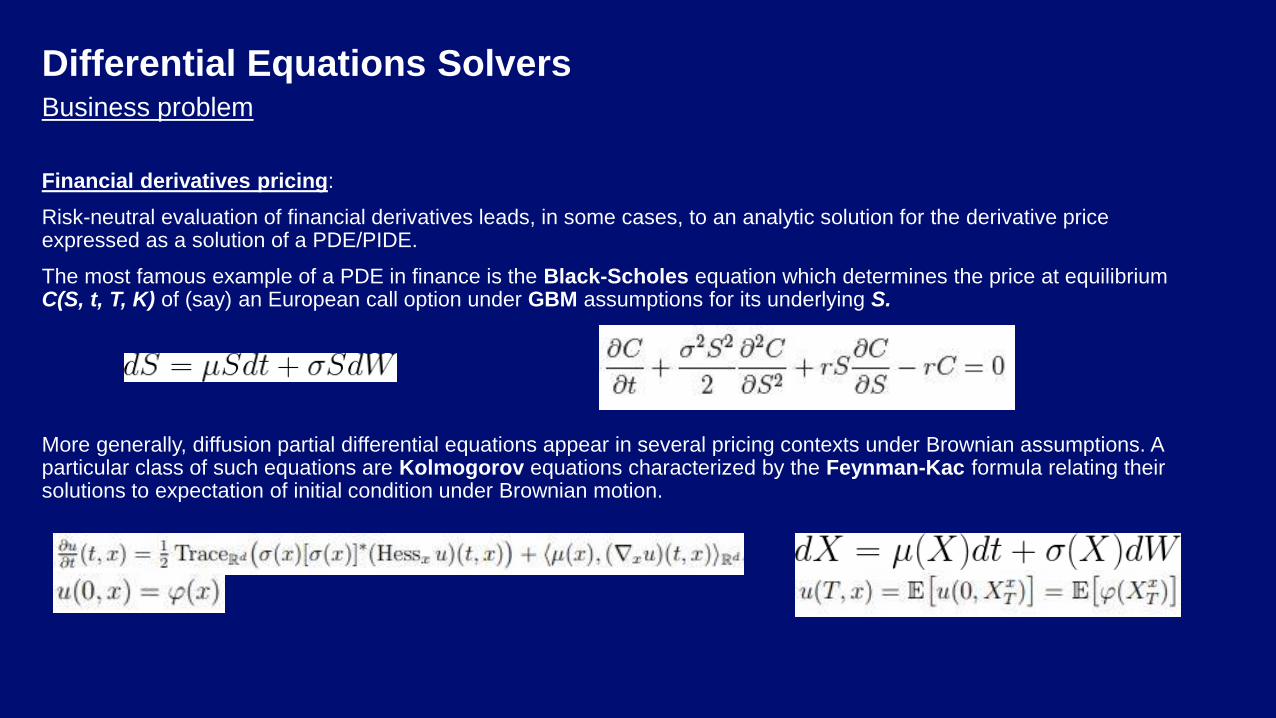
Financial derivatives pricing:

Risk-neutral evaluation of financial derivatives leads, in some cases, to an analytic solution for the derivative price expressed as a solution of a PDE/PIDE.

The most famous example of a PDE in finance is the Black-Scholes equation which determines the price at equilibriumC(S, t, T, K) of (say) an European call option under GBM assumptions for its underlying S.

More generally, diffusion partial differential equations appear in several pricing contexts under Brownian assumptions. A particular class of such equations are Kolmogorov equations characterized by the Feynman-Kac formula relating their solutions to expectation of initial condition under Brownian motion.


PIDEs arise in quantitative finance for risk-neural evaluation of financial derivatives under heavy-tailed dynamics (e.g. Lévyprocesses). For instance, under exponential Lévy assumptions for underlying S

where Xt is a Lévy process, the martingale property allows to determine a risk-neutral price in expectation that can be expressed as a solution of a partial integral equation of the form

This formulation in terms of PIDEs extends to other similar pricing frameworks under heavy-tailed (see for instance [1] for a detailed account).

[1]: R. Cont and P. Tankov, Financial Modelling with Jump Processes. Chapman and Hall, 2003.


Stochastic optimal control in finance:

Stochastic optimal control problems arise in several contexts in finance (portfolio allocation, Merton’s optimal investment-consumption problem, super-replication, optimal liquidation). Formally, a (discrete) stochastic optimal control problem is Markov Decision Process defined in terms of a state process Xt, a control process αt and a cost functional J

Stochastic optimal control problems lead to the Hamilton-Jacobi-Bellman partial differential equation for the value function of the problem u for some (possibly parametric) Hamiltonian H

Differential Equations SolversQF methods

Technique: Finite differences methods

Approximation numerical technique based on discretization of the partial (integral) differential equations. Fixed a grid in the equation variables and a discretization schema for differentials (implicit, explicit method), reduce the equation to a linear system solved starting from the known initial/boundary conditions.

Advantages:

• Largely adopted, consolidated

• Adaptable to a large number of types of equations

• Error analysis can be done analytically (e.g. using Taylor expansion)

Disadvantages:

• Curse of dimensionality: computational complexity generally grows exponentially with the number of variables of the equation.(some specific methods have been developed for certain type of equations to theoretically grant polynomial growth)

• Relies on linear estimates of both the coefficients and the solution of the equation on the grid of reference

• Grid choices affect stability of the solver

• Does not come with a default framework to also fit observed data while solving the equation

• Generally underperforms when the complexity of the equation grows (more variables, non-linear equations)

Differential Equations SolversDL methods

Technique: Deep Galerkin Method ([1])

Learning the solution to the equation as a neural network f in the variables minimizing the residual equation and boundary conditions error J(f)

Successfully implemented for different types of partial differential equations in the literature:

1. High-dimensional (200) free boundary Black-Scholes PDE [1]

2. High-dimensional HJB equation [1]

3. Derivatives pricing PIDE under Lévy processes (2]

4. Path-dependent derivatives pricing PDEs [3]

5. PDEs of relevance to physics: Burger equation, Schrödinger equation, General Stokes equations [4], [5]

[1]: J. Sirignano and K. Spiliopoulos, DGM: A deep learning algorithm for solving partial differential equations. Journal of Computational Physics 375(3), 2017.

[2]: A. Hirsa and W. Fu, An unsupervised deep learning approach in solving partial integro-differential equations, 2020..

[3]: Y. Saporito and Z. Zhang, Path-Dependent Deep Galerkin Method: A Neural Network Approach to Solve Path-Dependent Partial Differential Equations. SIAM J. Finan.

Math., 12(3) 2021

[4]: M. Raissi, P. Perdikaris, and G. E. Karniadakis (Part 1), Physics informed deep learning: Data-driven solutions of nonlinear partial differential equations

[5]: J. Li et al., The Deep Learning Galerkin Method for the General Stokes Equations, 2020.


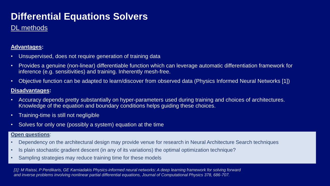
Advantages:

• Unsupervised, does not require generation of training data

• Provides a genuine (non-linear) differentiable function which can leverage automatic differentiation framework for inference (e.g. sensitivities) and training. Inherently mesh-free.

• Objective function can be adapted to learn/discover from observed data (Physics Informed Neural Networks [1])

Disadvantages:

• Accuracy depends pretty substantially on hyper-parameters used during training and choices of architectures. Knowledge of the equation and boundary conditions helps guiding these choices.

• Training-time is still not negligible

• Solves for only one (possibly a system) equation at the time

Open questions:

• Dependency on the architectural design may provide venue for research in Neural Architecture Search techniques

• Is plain stochastic gradient descent (in any of its variations) the optimal optimization technique?

• Sampling strategies may reduce training time for these models

[1]: M Raissi, P Perdikaris, GE Karniadakis Physics-informed neural networks: A deep learning framework for solving forward

and inverse problems involving nonlinear partial differential equations, Journal of Computational Physics 378, 686-707.


Technique: Neural Operator learning

Supervised learning approach to learn a (typically non-linear) operator mapping between two infinite dimensional spaces (of functions) from a finite collection of observations of input-output pairs.

In the context of differential equations, the operator maps parameters/boundary conditions for the problem to the associated solution.

Fourier layers, introduced in ([2]), have shown promising results in such infinite dimensional setup for Burger’s equation, Darcy flow and Navier-Stokes equations. Neural network learns a kernel for the equation in Fourier space.

[1]: L. Lu, P. Jin, and G. Karniadakis. Deeponet: Learning nonlinear operators for identifying differential equations based on the universal

approximation theorem of operators. 2019

[2]: Z. Li et al., Fourier neural operator for parametric PDEs, 2021.


Advantages:

• More scalable since it can solve a family of equations rather than one at the time

• Resolution/mesh independent

Disadvantages:

• Supervised, relies on training data generation that must come from classical solver (reported for Navier-Stokes 10k samples)

• Operates in infinite dimensional space hence theoretical convergences guarantees might be weaker

Plots: Neural solver Black-Scholes PDE

GS CoreAI RDE Demo

(orange) Model prediction

(blue) Analytic BS solution

Remarks

Curse of dimensionality:

As of today, there is no general theorem proving that neural network based techniques overcome the curse of dimensionality. However, there has been intermediate proof for certain classes of PDEs:

• Grohs et al. ([1]) proved that there exist neural network approximation for solution of linear Black-Scholes PDEs with number of parameters growing at most polynomially in both the reciprocal approximation accuracy and the PDE dimension.

• Hutzenthaler et al. ([2]) extends this result to semi-linear heat PDEs with Lipschitz continuous nonlinearities

Desirable: empirical study of computational performance of these models stratified by equation type, dimensionality, dataset size and architectural complexity. Same for MC replication problems.

[1]: P. Grohs et al., A proof that artificial neural networks overcome the curse of dimensionality in the numerical approximation of Black-Scholes partial differential

equations, 2018.

[2]: M. Hutzenthaler et al., A proof that rectified deep neural networks overcome the curse of dimensionality in the numerical approximation of semi linear heat

equations. SN Partial Differential Equations and Applications 1 (2020), 1–34.

Representation learning vs function fitting:

Applications of deep learning usually rely on the notion of representation learning. Deep neural networks have shown the ability to automatically engineer intermediate features representing, for instance, semantic or visual ques from raw data. Increasing number of layers allows the model to refine these representations resulting typically in better performance.

In the applications so far described, is somewhat unclear what representation learning means. These tasks resemble more of a function fitting problem provided explicit features/variables (e.g. spot prices, tenors, etc.). This could explain, for instance, more rigid dependency on the choice of an architecture for the problem.

Neural strategies

Neural strategiesBusiness problem

Determine an optimal policy/decision with respect to a given objective which depends on some observation of a state of the system.

Hedging of financial derivatives:

Hedging strategy involves determining optimal portfolio allocation across different assets (typically some underlying and derivatives) to minimize (hedge) risk-exposure of the portfolio.

Derivative contracts are commonly used for hedging. The most common liquid contracts are: future contracts, options and swaps. Hedging can involve also non-liquid exotic contracts for which the determination of an hedging strategy can be more challenging.

Portfolio management:

In the context of Asset Management trading strategies attempt to optimize a certain metric (e.g. Sharpe ratio) to attain optimal frontier portfolios.

Stochastic optimal control in finance:

Stochastic optimal control problems, as previously discussed, arise in several contexts in finance (portfolio allocation, Merton’s optimal investment-consumption problem, super-replication, optimal liquidation). In this context we can talk about a strategy that solves the optimal control.

Neural strategiesQF methods

Technique: Stochastic calculus

Quantitative finance and stochastic calculus allow, under simplified assumptions, to determine analytic solutions to the hedgingproblem. For instance, consider a portfolio involving an underlying asset S and a call option C on S and assume that S is modeled by the (GBM) SDE:

Ito's calculus and Black-Scholes pricing theory provide an exact analytic hedge (delta-hedging) of the portfolio against movements of S.

Advantages:

• Analytic nature allows to have confidence about the hedged risk

Disadvantages:

• For more complex products, stochastic models and risk factors, determining an analytic solution to this problem can be challenging. In practice, hedges can be calculated numerically from sensitivity analysis of pricing engines

• Under more realistic assumptions (e.g. transaction costs, incomplete markets) an exact theoretical hedge may not be determined (see [1]) which leads to the formalization of the problem in terms of risk-preferences theory

• Challenging modeling of other features, such as news, that could impact market prices

[1]: H. M. Soner, S. E. Shreve and J. Cvitanić, There is no Nontrivial Hedging Portfolio for Option Pricing with Transaction Costs, The Annals of Applied Probability Vol. 5,

No. 2 (May, 1995)

Neural strategiesDL methods

Technique: Local optimization: risk-sensitive reinforcement learning

Reinforcement learning (possibly DeepRL) algorithms rely on:

1. MDP with a local reward function R(s,a)

2. Solving the Bellman’s equation via estimation of a Q(s,a) or a value V(s) function

In the context of risk-management (hedging) and portfolio optimization, a local risk-adjustment of the reward R(s,a) must be provided to the algorithm to meet prescribed risk minimization objectives.

The main theoretical references are risk-sensitive and risk-constrained reinforcement learning

• Risk-sensitive RL: objectives are augmented with a local-risk penalty to adjust the agent rewards (see for instance [1], [2]).

• Risk-constrained RL: the risk penalty is induced by a constrained optimization problem that leads, via a Lagrangian formulation, to the adjustment of the reward (see for instance [3], [4]).

[1] Y. Shen, M. J. Tobia, T. Sommer and K. Obermayer, Risk-sensitive Reinforcement Learning, Available at arxiv 1311.2097

[2] L. Bisi, L. Sabbioni, E. Vittori, M. Papini and M. Restelli, Risk-Averse Trust Region Optimization for Reward-Volatility Reduction, Available at arxiv 1912.03193

[3] A. Tamar, Y. Chow et al., Policy Gradient for Coherent Risk Measures, Advances in Neural Information Processing Systems 28 (NIPS 2015)

[4] C. Tessler, et al. Reward Constrained Policy Optimization, In Proc. of the 7th International Conference on Learning Representations, ICLR19, 2019


Algorithms in this framework have been proposed In the context of hedging :

1. Q-learning algorithm (QLBS) for hedging based on risk-adjusted returns for an option replicating portfolio, as in the Markowitz portfolio theory ([1])

2. Deep DPG algorithm for hedging based on quadratic risk-adjustment ([2])

3. TRVO algorithm for hedging based on quadratic risk-adjustment ([3])

4. Policy gradient and actor-critic algorithms constraint on the conditional value-at-risk ([4])

[1] I. Halperin, QLBS: Q-Learner in the Black-Scholes(-Merton) Worlds, 2017. Available at SSRN 3087076.

[2] J. Cao, J. Chen, J. Hull and Z. Poulo, Deep Hedging of Derivatives Using Reinforcement Learning, 2021. Available at SSRN 3514586.

[3] E. Vittori, M. Trapletti and M. Restelli, Option Hedging with Risk Averse Reinforcement Learning, Available at SSRN 3514586.

[4] Y. Chow, M. Ghavamzadeh et al., Risk-Constrained Reinforcement Learning with Percentile Risk Criteria, Journal of Machine Learning Research 1, Vol. 18, No. 1


Advantages:

• Provide more flexibility in terms of the risk-objective which is local in the state

• Can handle real-markets phenomena such as transaction costs, liquidity, etc.

• Deep RL techniques come with non-linearity, high-dimensionality and a flexible notion of a state that can be adapted to other features (e.g. news vectorization).

Disadvantages:

• Algorithms do not ensure risk guarantees at a global (trajectory) level

• Choices of risk parameters can be challenging

Open questions:

• Determining locally adjusted algorithms that can ensure risk-management guarantees at a global (trade) level


Technique: Global optimization

Global optimization techniques solve for an optimal strategy via direct policy search: cumulative rewards over batches of trajectories are aggregated and fed into a risk-adjusted objective which induces the risk-preferences for the strategy. Neural agent parameters are updated via direct back-propagation.

An example of application of this technique to hedging is Deep Hedging [1], where the class of convex risk-measures is considered. Among these, entropic risk measure (corresponding to exponential utility) and CVaR

This approach has been recently extended in [2] to the class of translational invariant risk measure.

Global optimization techniques have been tested also in the context of asset management (see [3]) where the optimization objective is a Sharpe ratio metric.

[1] H. Buehler, L. Gonon, J. Teichmann and B. Wood, Deep hedging, Quantitative Finance, 1-21.

[2] A. Carbonneau, F. Godin, Deep equal risk pricing of financial derivatives with non-translation invariant risk measures, 2021

[3] J. Wang et al. , AlphaStock: A Buying-Winners-and-Selling-Losers Investment Strategy using Interpretable Deep Reinforcement Attention Networks, KDD '19:

Proceedings of the 25th ACM SIGKDD International Conference on Knowledge Discovery and Data Mining July 2019


Advantages:

• Provides a global-aware optimization (at a trade level)

• Easy to factor in real-markets frictions (transaction costs, liquidity, etc.)

• Includes the class of short-fall risk in the optimization objectives

• Could be used for more complex products

Disadvantages:

• Relies on a simulation engine for the liquid instruments that the agent trades

• Easier to tune when a known a risk-neutral probability measure is givenPlots: Neural Black-Scholes delta hedging replication

GS CoreAI RDE Demo

Open questions:

• Efficiency of SGD for this task, explore gradient-free optimization applied in RL (e.g. evolution strategies)

• Determine a price from the hedge (proposal under equal risk pricing framework without transaction costs [1])

• Determine algorithmically a risk-neutral measure from the physical measure (proposal [2])

[1] A. Carbonneau, F. Godin, Deep Equal Risk Pricing of Financial Derivatives with Multiple Hedging Instruments, 2021.

[2] H. Buehler et al., Deep Hedging: Learning Risk-Neutral Implied Volatility Dynamics, 2021. Available at SSRN 3808555

Modeling of financial time-series

Modeling of financial time-seriesBusiness problem

Time-series modeling:

Most of the methodologies (both currently used or AI based) discussed so far rely on a simulation engine for financial time-series to simulate paths for statistical computations or learning.

Key feature for any simulation engine is the ability to replicate empirical statistics of observed time-series. These features are known in the literature as stylized facts. For assets returns (see [1]), most salient observed statistics are:

• autocorrelations (linear) are often insignificant

• (unconditional) distribution displays a power-law or Pareto-like tail (heavy tails)

• volatility display a positive autocorrelation over several days (volatility clustering)

• ACF of absolute returns decays slowly as a function of the time lag

• measures of volatility are negatively correlated with returns (leverage effect)

Further, time-series can express non-linear relations as for the case of price-volumes (see [2]).

Figs Credit: [1] R. Cont, Empirical properties of asset returns: stylized facts and statistical issues, Quantitative Finance Vol. 1 (2001), pp. 223-236.

[2] S. Behrendt, A. Schmidt, Nonlinearity matters: The stock price-trading volume relation revisited, Economic Modelling Vol. 98, 2021.

Modeling of financial time-seriesQF methods

Technique: Calibration of stochastic processes

Standard practice involves assuming a stochastic model for the time-series and calibrating its parameters to observed data (e.g.Euler-Murayama schema). Most common stochastic processes are GBM, Heston stochastic volatility model, Vasicek model, Hull-White model, GARCH models.

Advantages:

• Consolidated practice with a sound statistical theory

Disadvantages:

• Relies on a statistical prior assumption about the distribution

• More complex stochastic models can lead to computational over-heads

• Non-linear relations may be weakly captured

• Statistical theory weakens outside of ‘Gaussian world’, especially with respect to heavy-tailed distributions

Modeling of financial time-seriesDL methods

Technique: Deep generative modeling of financial time-series

Deep generative models have been recently developed and tested for simulation of financial time-series data. Originally developed for generation of images, language and audio, they appear to provide a viable path for simulation in finance.

These are unsupervised models based on neural architectures such as VAEs (variational auto-encoders) or GANs (generative adversarial networks).

Specific applications to financial modeling include:

• WGAN, DCGAN, RegGAN (see [1])

• VAE, CVAE under scarce data regimes (see [2])

• Autoregressive GAN for option prices (see [3])

• TCN (WaveNet) (see [4])

[1] G. Di Cerbo, A. Hirsa and A. Shayaan, Regularized Generative Adversarial Network, Available at SSRN 3796240.

[2] H. Buhler, B. Horvath, T. Lyons et al., A Data-Driven Market Simulator for Small Data Environments, Available at SSRN 3632431, June 21, 2020.

[3] M. Wiese, et al. Deep Hedging: Learning to Simulate Equity Option Markets, NeurIPS 2019 Workshop on Robust AI in Financial Services, 2019.

[4] M. Wiese, R. Knobloch, R. Korn and P. Kretschmer, Quant GANs: deep generation of financial time series, Quantitative Finance Volume 20, 2020 - Issue 9.

Figs Credit: T. Karras et al., A Style-Based Generator Architecture for Generative Adversarial Networks, 2019 IEEE/CVF Conference on Computer Vision and Pattern

Recognition (CVPR)


GANs (Generative Adversarial Networks) are characterized by two neural networks called the generator and the discriminator. Given distributions X and Z (X is an observed distribution and Z is a latent stochastic code)

• Generator G attempts to produce, for each sample z in Z, an element G(z) close in distribution to elements of X

• Discriminator D attempts to discriminate between samples generated by G and natural samples of X

More specifically, GAN optimization is achieved through solving a min-max problem of the form:

Temporal convolutional neural networks (WaveNet [1]), originally developed for audio processing, have been tested in a GAN framework for financial time-series generation in [2] highlighting the relevance of encoding temporal correlation via a prescribed architectural bias of the generator network.

Experimental evidence provided shows that this model out-performs GARCH in reproduction of stylized facts for S&P500returns

[1] A. van den Oord et al., Wavenet: A generative model for raw audio, 2016.

[2] M. Wiese, R. Knobloch, R. Korn and P. Kretschmer, Quant GANs: deep generation of financial time series, Quantitative Finance Volume 20, 2020 - Issue 9.


Architectural biases appear to be able to represent some stylized facts depending on the temporal structure of the time-series.

How about heavy-tailed distributions?

A pretty general theoretical result of [1] states that Lipschitz continuous functions (in particular C^1 functions) cannot change the tail behavior of the input distribution.

This implies, in particular, that (any) GAN cannot generate an heavy-tailed distribution from Gaussian latent code.

The authors address this issue by sampling from a Pareto latent code. Further, they propose a method based on extreme value theory for tail-index and loss function parameters selection.

Figs Credit: [1] T. Huster et al., Pareto GAN: Extending the Representational Power of GANs to Heavy-Tailed Distributions, ICML 2021.


Advantages:

• Model free, does not require strong assumptions on the modeling

• Can recover some stylized facts

• Architectural biases have representational power for temporal structure and to express non-linearity

Disadvantages:

• Require medium to large datasets for training, computationally intense to train

• GANs are notoriously hard to train (collapse mode) hence could require intense hyper-parameters search

Open questions:

• Latent noise distribution affects the statistics of data generated, how to effectively use heavy-tailed noise for accurate reproduction of tails and overcome their underrepresentation

• Develop architectures that canonically capture cross-sectional correlation structure

Final Remarks

A possible venue for interaction of techniques and theories:

Classical quantitative finance is founded on a very rigorous statistical and mathematical theory which determines a certain degree of rigidity.

Deep learning, on the other hand, is a flexible, multi-purpose, data driven technique whose foundations are to some extent still not well understood.

A possible outcome of this interaction, as the two approaches converge, could lead to a better assessment of both frameworks weaknesses. On a speculative note:

• Fitting well defined mathematical problems with neural networks could lead to a better understanding of learnability in a more general context

• Rigorous knowledge of statistical modeling in quantitative finance could benefit understanding and modeling training dynamics inneural network weights

• Development of risk-aware RL frameworks could extend outside the scope of finance (e.g. risk-aware RL in autonomous navigation and robotics)

Statistical Mathematical Theory

Data drivenQF DL

Documents

New frontiers in deep learning and quantitative finance