NEW EXPLICIT MICROPLANE MODEL FOR CONCRETE : THEORETICAL ASPECTS AND

NUMERICAL IMPLEMENTATION

IGNACW CAROL* and PERE C. PRATT School of Civil Engineering. ETSECCPB-Technical l!nivcrsit! ef C;rt;dania.

OXfl?-t Barc&wn. Spain

I. INl’KOI>UCTION

In ic)3S, G. 1. Taylor suggested ;I new class of materiul ~nockls for plastic polycrysttlllinc

metals in which the constitutive material properties arc ~h~ir~~~t~ri~~d by relations hctwccn

the stress and strain ~~?rnpon~nts on planes of vurious ~ri~nt~lti~ns in the materiaf (now

called the microplancs). which arc constrrtinrd either staticrtlly or ~in~rn~lti~~llly to the

macro-stress or mitcr+stritin. fktsccl on the statio constraint. this basic icloa has been

extcnsivcly dcvrlopcd for mctitls under the n;lmc of slip theory. beginning with the pion-

ccring work of Butdorf and Hudiunski (1939). Lutcr. the models with static constraint have

been iiditptcd for gcomatcrials (Zienkicwicz and Park, 1977; Pandc ilnd Sharmit. 1983).

In ;lpplication to concrete and gcomatcrials. the name “slip theory” bccumc misleading

bccausc most of the inclustic rcsponsc is due to dam:tgc such as microcracking. and the

rnl>rc gcncrrtl term “misropfanc modci” was coined (Uahnt itncf Oh, 19Y3 ; fk&mt. 1984).

f t was ills0 rccognizfd that the str~~in-s~~~.t~nin~ obscrvcd in ~~~~~l~~&~riillS CittlilOt bC rep-

rescntcd with ;t static constr~~int bcc:~usc the nli~r~~pli~n~ system becomes unstable, and

conscqucntly ;L kinematicconstraint has hctn adopttXi (f3a%unt and Oh. 19X3, 1985; Buiitnt,

1984: BitPant and Gamharova. IWJ: Ikti.itItt :tnd f’ritt. IVXX). although ;I more gcncral

mixed constraint might conceivably also bc used.

The microplanc model with kinematic constraint and strain-softening hiis proved to

bc a powerful approach for modcfling rather complex aspects of trianial hchavior of

t Formerly Vkiting Scholars. Ccnbx for Advanced Ccmcnt-kwd M:~tcrials. Northweslcrn University.

Evanston. IL 6020X. U.S.r\.

1173

Inr j ..... dfd .. S[r~,!l.4rn\,li..=tJ.'n ~.rr 11"'3··11\)1. !oN":

Pnnh.:d In Great Bnt.un. on=:o ~oJ\) Q~ S5 on .. .till

I I!.N: Pcrgamnn Prc!.s pk

NEW EXPLICIT MICROPLANE MODEL FOR CONCRETE: THEORETICAL ASPECTS AND

NUMERICAL IMPLEMENTATION

IG~AClO CAROlt and PERE C. PRATt &hool ofCivi\ Engineering. ETSECCPB-Technical Universit~ "fCltalonia.

oxn:;~ Barcdona. Spain

and

ZDE~i:K P. BAZA~T IXpartment of Civil Engin~-.:ring. Center for Adv<ll1l.:ed Cement-Based Materials,

:"-iorthwestern University, Ev,\Oston, IL 601Ut(, U.S.A.

(Rccdl'{·tl:! Arri/1990; ill rt'l"isecl.li.rm 10 .lu{llIsl t991l

Ailstract-The microplane mood is a powerful ,tppruach for the represent;ttillll of the complex triaxial behavior of concrete and other similar materials. 1I0wev.:r. most drorls in pfl'vil'us for­mutations were devoted to the devdopment of the modd ilsdf ami 10 Ihe e:l.perilllental ~hlla lilting. rather than to a eomprch"nsive theoretie.iI deseriptilln or tll atl.tinl1lent or ,I nl\,dlliar and wmputatillllally etlki,'nt implementatioll in a <:,l(l1puh:r <:"de. In this paper. these l,bjel:tives arc pursued. The rormulati,)(1 or the nwdd has heen Illodified 10 rationali/e the stru<:lure uf the oasil: hypolheses. simplify Ihe equatill(lS ami genera life the eOIll.:epl, whenever po"iolc. The result is a new formulalion which. while relaining the l;lVt,r;IOlc properlies achieved previullsly. is alsll easier I" ul1lkrst;lIlll. and coovenicnt f"r computer implement<lti"n and large-seak c;lkulalions. A COIll­putational schemc is prcsentell wilh the lInilicd structurc or a g<:ncr;t1 <:odc serving thc dl,uolc purposc of test spel:imen an<llysis aflll tillite dement <lnalysis. III praclice. Ilti~ ~tructure includes two dillercnt l1l;tin programs which callthc same sct of conslitutive slIoroutines. t\ salicnt lealurc of the new version of Ihe modd is thaI the C()f1IPllt;llioll of the stress corrcsponding to a prescrihct! strain inen:m<:nt of linitc si/c is fully explicit. Slcp-oy-s":p numcncal inlegr;lliul1. uSII;llly lleceS'ary fur the pmcticaillse of conslitutive mudds. can he avoided. ('onscqll!:nlly. the clllllpkxily of the colle and Ihe Cllst or COl1lput;!tiollS call he ~Iram'llic;tlly rcdl\l.:cd. SlIlIle c.\ampics of apI>hcatiolls, used III verify th.: pn:violls version of Ih.: mudd. ;Ire ;tlso prcscnt.:d. They dClllonstrate that this ncw formulation gives a Illuch hcllcr numcrical dlicien<:y for code impklllclllatioll while k.:.:ping th.: salllc ~ksirahlc leatur.:s and accur;!cy in .:xpcrimcntaillata lilling.

I. INTRODUCTION

In t93X. G. l. Taylor suggested a new class or material models for plastic polycrystalline metals in which the constitutive material properties arc characterized by relations between the stress and strain components on planes of various orientations in the material (now called the microplanes). which arc constrained eithcr statically or kinematically to the macro-stress or mm.:m-strain. Based on the static constraint. this basic idea h~IS been extensively developed for metals under the name of slip theory, beginning with the pion­eering work of Batdorf and Budianski (1949). Luter. the models with static constraint have been adapted for geomateriuls (Zienkiewiez and Pande. 1977; Pande and Sharma. 1983). In application to concretc and geomaterials, the name "slip theory" became misleading because most of the inelastic response is due to damage such as microcrucking, and the more general term "microplane model" was coined (Bazant and Oh. 19M3; Bazanl. (984). It was also recognized that the strain-softening observed in geomaterials cannot be rep­resented with a static constraint because the microphlllc system becomes unstablc, and consequently a kinematic constraint has been .tdopted (Bazant and Oh, 19X3. 19X5; Ba7::lIlt. 1984: Bazant and Gamharov<l, 19X4: Bazanl and Prat. 19XX). although a mort:: general mixed constraint might conceivably also be used.

The microplane model with kinematic constmint and strain-softening has proved to be a powerful approach for modelling rather complex aspects of tri'lxial behavior of

t Formerly Visiting Scholars. C.:nter ror Advanced Cement-Based Materials. Northwestern University, Evanston, IL ('020~. U.S.A

117-'

1174 I. CAKOL Cl ul.

brittle-plastic materials such as concrete. rock. ceramics and some composites (Baiant and

Gambarova. 1984; Baiant and Oh. 1985; Baiant and Prat. 1988; Baiant and Oibolt.

1990). However, as usual in the exploration of new constitutive models. most attention has

so far been paid to achieving an accurate representation of the main aspects of material

behavior given by experimental curves rather than to other theoretical or numerical aspects

also important for constitutive modelling.

Further work has lead to the conclusion that the theoretical description of the model

given in previous works can be simplified. the same concepts can be presented in a more

comprehensive way, and a new and clearer interpretation of some of the equations and

variables involved in the formulation is possible. Also, some derivations can be given a

more rigorous or alternative description, and some changes can be made in the hypotheses

and assumptions, so that the final formulation is better suited for practical application.

From the viewpoint of numerical implementation and code development. the previous

formulations of the microplane model also lacked a systematic approach. In general. the

computer implementation of a constitutive model is undertaken with one of the following

two purposes: (i) representation of the material behavior itself. as a relationship between

stress and strain (“single-point constitutive verification”). or (ii) representation of the

material behavior in the context of structural analysis (“F.E. analysis”). Without ;I unitied

scheme of implementation, the programs developed for these two purposes may well have

completely different structures, and the part of the code corresponding to the constitutivc

model may feature two completely different implementations of the same model. which in

a way was the case for the previous versions of the microplane model.

In this paper both aspects, a new theoretical description (Section 7) and ;I new numerical

imptcmcntation scheme (Section 3) for the microplane model, arc prcscnted. Altogether,

these aspects yield a new version of the model which, while keeping all the useful features

achieved in the previous version in terms of constitutivc verification. is also casicr to

understand and better suited for practical use in the context of a general F.E. code. The

new computer schcmc includes two model-indcpcndcnt main programs calling the s;unc

material subroutine which gives ;LCCCSS LO all the model-specific routines and computations.

In this way, all the inconveniences caused by having two dilfercnt programs implementing

the same model are overcome automatically : the code needs to he written only once. and

once verified at the constitutive level it is automatically working for I:.E. computations.

Moreover, any further modifications introduced to the model need to bc cncodcd only once.

Thus. both the single-point and F.E. analysis programs always contain the sarnc version of

the model, and the results obtained from both levels of analysis arc fully consistent for

comparison or complementary use in the same practical problem. By virtue of the general

scheme used and the new theoretical assumptions for the modct, the computations in these

subroutines (which basically must perform a load-stepcomputation from prescribed strain)

are fully explicit, without any step-by-step integration procedure. This makes the code

simple to implement and fast to run.

Section 4 presents some examples. The results obtained arecompared with expcrimcntnl

data and published results of the previous version of the microplane model. The comparison

is made in terms ofcapability to fit experimental data as well as numerical efficiency. Fimtlly,

Section 5 gives a brief summary and the main conclusions drawn from this work.

2. TIIEORETICAL DESCRlPTtON OF THE EXPLICIT MICROPLANE MODT:L

At a point within the material, a microplane is defined as an arbitrary plane which cuts

through the material at that point, defined by the orientation of its normal unit vector of

components n,. The most direct and easiest physical interpretation of a microplane comes

from the observation of the material microstructure, as the interface or discontinuity plane

between grains or different components in the heterogeneous medium (Batant and Gambarova.

1984; Baiant and Oh, 1985; Baiant and Prat. 1988).

On a generic microplane. certain components of strains and stresses are considered.

These are the normal and shear strains and stresses on that plane. A set of stress-strain

laws are defined as the relations between strains and stresses on the microplane. These laws,

IIU L CAROL 1ft ul.

brittle-plastic materials such as concrete. rock. ceramics and some compositt:s (Bazant and Gambarova. 1984; Baiant and Oh. 1985; Baiant and Prato 1988; Bazant and Ozbolt. 1990). However. as usual in the exploration of new constitutive modds. most attention has so far been paid to achieving an accurate representation of the main aspt:cts of material behavior given by experimental curves rather than to other theoretical or numerical aspects also important for constitutive modelling.

Further work has lead to the conclusion that the theoretical description of the model given in previous works can be simplified. the same concepts can be presented in a more comprehensive way. and a new and clearer interpretation of some of the equations and variables involved in the formulation is possible. Also. some derivations can be given a more rigorous or alternative description. and some changes can be made in the hypotheses and assumptions. so that the final formulation is better suited for practical application.

From the viewpoint of numerical implementation and code development. the previous formulations of the microplane model also lacked a systematic approach. In general. the computer implementation of a constitutive model is undertaken with one of the following two purposes: (i) representation of the material behavior itself. as a relationship between stress and strain ("single-point constitutive verification"). or (ii) representation of the material behavior in the context of structural analysis ("F.E. analysis"). Without a unified scheme of implementation. the programs developed for these two purposes may well have completely different structures. and the part of the code corresponding to the constitutive model may feature two completely different implementations of the same model. which in a way was the case for the previous versions of the microplane model.

In this paper both aspects. a new theoretical description (Section 2) and a new numerical implementation scheme (Section 3) for the microplane model, arc presented. Altogether. these aspects yield a new version of the model which. while keeping all the useful features achieved in the previous version in terms of constitutive verification. is also easier to understand and better suited for practical usc in the context of a general F.E. code. The new computer scheme includes two model-independent main programs calling the sallle material subroutine which gives access to all the model-specific routines and computations. In this way. all the inconveniences caused by having two different programs implementing the same model arc overcome automatically: the code needs to he written only once. and once verified at the constitutive level it is automatically working for F.E. wmputations. Moreover. any further modifications introduced to the model need to he encoded only once. Thus. both the single-point and F.E. analysis programs always contain the same version of the model, and the results obtained from both levels of analysis arc fully consistent for comparison or complementary use in the same practical problem. By virtue of the general scheme used and the new theoretical assumptions for the model. the computations in these subroutines (which basically must perform a load-step computation from prescribed strain) are fully explicit, without any step-by-step integration procedure. This makes the code simple to implement and fast to run.

Section 4 presents some examples. The results obtained are compared with experimental data and published results of the previous version of the microplane model. The comparison is made in terms of capability to fit experimental data as well as numerical elliciency. Finally, Section 5 gives a brief summary and the main conclusions drawn from this work.

2. THEORETICAL DESCRIPTION OF THE EXPLICIT MICROPLANE MODEL

At a point within the material. a microplane is defined as an arbitrary plane which cuts through the material at that point. defined by the orientation of its normal unit vector of components n,. The most direct and easiest physical interpretation of a microplane comes from the observation of the material microstructure. as the interface or discontinuity plane between grains or different components in the heterogeneous medium (Bazant and Gambarova. 1984; Bazant and Oh. 1985: Bazant and Prato 1988).

On a generic microplane. certain components of strains and stresses are considered. These are the normal and shear strains and stresses on that plane. A set of stress-strain laws are defined as the relations between strains and stresses on the microplane. These laws,

Yew explicit microplane model for concrete II75

together with the relations between macroscopic and microplane stresses and macroscopic

and microplane strains. constitute the material model.

2. I. Kinematicail~ construinetl microplune s_wem In the first models of this type developed for metals and soils. a static constraint (the

microplane stresses are equal to the resolved components of the stress tensor on that plane)

was assumed as the fundamental micro-macro relationship. However. to represent the

behavior of quasibrittle materials such as concrete or rock. showing strain softening. a

kinematic constraint (the microplane strains are equal to the resolved components of the

strain tensor on the plane) seems to be necessary. As will be shown in Section 3. this

assumption fits very well into the strain-to-stress scheme used for numerical calculations

and makes possible fully explicit types of calculations with great economy in computer

time.

The theoretical framework for the new explicit microplane model is based on the three

hypotheses given below, similar to those used by Baiant and Prat (1985). with some changes

that affect the resulting formulation and its numerical implementation :

H.yotltcsis 1. The normal and shear (tangential) strains cs and cr on a microplane of

unit normal II, arc the resolved components of the macroscopic striin tensor E,, in that

direction. which implies that

+ = 1:,,tr,n, (1)

Er = f:,,tt, -i:~tt, = (h,, -tt,tt,)ttAt:,k. (‘I

Additionally. the normal strain is split in two parts. the volumetric strain I:~ and the (normal)

dcvintoric strain I:,,. the cxprcssions of which arc

t:,, = 1:s -I:“. (J)

The latin lowercase subscripts rcfcr to Car&an coordinates .r,(i = I. 3. 3). and subscript

ropstition implies summation.

Note that the tangential strain is II vector with three components in space, but its

direction always lies in the microplane of normal n, [(cheek that Er,tt, = 0, from cqn (?)I.

Also the normal strains are vectors with three Cartesian components in the normal direction

II,, though only their magnitudes c.+ t:” and El, arc used. A useful alternative interpretation

of the variables E”, t:,, and E,., can bc obtained if they are dcrivrd in terms of the volumetric

.Q and dcviatoric v,, = I:,, -t:vS,i pilrts of the macroscopic strain instead ofdircctly from the

tensor t:,,. Then. the volumetric strain at microplanc lcvcl G,. which is the same for all the

microplancs, is directly equal to the macroscopic volumetric strain. The normal deviatoric

strain E,, and the tang~ntii~l strain c,,. which ilrc dilTixcnt for each microplane, arc equal to

the normal and tangential components of the projection of the dcviatoric strain tensor. v,,.

on the microplanc considcrctl.

tf~pothcsis II. Associated with the three strains cv. c,, and Er,. the three corresponding

stresses gv. (r,, and ur, arc introduced so that their rcspcctivc products give directly the

work done on the microplanc. The strain--stress laws at this Icvcl arc a set of empirical

relationships defining the evolution of each one of those three strcsscs as a function of the

three microplanc strains (and possibly their history) exclusively.

The fact that the laws for cv. CT,, and cr,, ilK functions of strains cnclusively is a very

important difl’crence with the previous version of the model (Baiant and Prat, 1958). This

hypothesis permits the model to bc fully kincmatically constrained. Consequently, other

kinds ofdependences. such as the dependence of OTT, on a certain invariant of the macroscopic

".:W .:xplicit microplanc: model for concrete: 1175

together with the relations between macroscopic and microplane stresses and macroscopic and microplane strains. constitute the material model.

2.1. Kinematically constrained microplane system In the first models of this type developed for metals and soils. a static constraint (the

microplane stresses are equal to the resolved components of the stress tensor on that plane) was assumed as the fundamental micf<rmacro relationship. However. to represent the behavior of quasibrittle materials such as concrete or rock. showing strain softening. a kinematic constraint (the microplane strains are equal to the resolved components of the strain tensor on the plane) seems to be necessary. As will be shown in Section 3. this assumption fits very well into the strain-to-stress scheme used for numerical calculations and makes possible fully explicit types of calculations with great economy in computer time.

The theoretical framework for the new explicit microplane modd is based on the three hypotheses given bdow. similar to those used by Baiant and Prat (1988). with some changes that affect the resulting formulation and its numerical implementation:

Hypothesis I. The normal and shear (tangential) strains t:~ and f.r. on a microplane of unit normal ", arc the resolved components of the macroscopic strain tensor f.il in that direction. which implies that

( I )

(2)

Additionally. the normal strain is split in two parts. the volumetric strain f., and the (normal) deviatork strain I:". the expressions or which arc

(3)

(4)

The latin lowercase subscripts refer to Cartesian coordin'ltes x,(i = I. 2. 3). and subscript repetition implies summation.

Note that the tangential strain is a vector with three components in space. but its direction always lies in the mieroplane of normal n, [(check that I:r", = n. from eqn (2)). Also the normal strains arc vectors with three Cartesian components in the normal direction ",. though only their magnitudes f.~. I:v and t:() arc used. A useful alternative interpretation of the variables I:v. I:() and f.r, can be obtained if they arc derived in terms of the volumetric f.y and deviatoric e" = /:" -I:y()'i parts of the macroscopic strain instead of directly from the tensor I:,/, Then. the volumetric strain at microplane level f.y. whieh is the same for all the mieroplanes. is directly equal to the macroscopic volumetric strain. The normal deviatorie strain ell and the tangential strain I:", which arc different for each microplane, arc equal to the normal and tangential components of the projection of the deviatoric strain tensor. e".

on the microplane considered.

Hypothesis II. Associated with the three strains f.y. f.1l and I:r,' the three corresponding stresses (Jv. (Ju and (Jr, .Ire introduced so that their respective products give directly the work done on the microplane. The strain--stress laws at this level arc a set of empirical relationships defining the evolution of each one of those three stresses as a function of the three microplane strains (and possibly their history) exclusively.

The fact that the laws for (Ty. (Til and (Tr, arc functions of strains exclusively is a very important difference with the previous version of the model (Bazant and Prat, 1988). This hypothesis permits the model to be fully kinematically constrained. Consequently. other kinds of dependences. such as the dependence of fTT, on a certain invariant of the macroscopic

1176 1. CAROL Cl Ui

stress tensor assumed in previous works (which in fact established a “mixed” kinematic-

static constraint for the model) are in this case excluded from the formulation.

Hypothesis II/. The relationship between the microplane stresses bv. c,, and oT, and

the macroscopic stress tensor a,, is obtained by applying the principle of virtual work. Its

application to this case is explained in some detail in Appendix A. including certain

considerations about symmetry requirements for the tensors a,, and E,, necessary to ensure

interchangeability of the indices iandjin the final expressions (the symmetry considerations

used in the Appendix are an alternative to the a priori symmetrization of eqn (2) used in

previous works to reach the same final effect). The expression for the macroscopic stress is

then :

s ;(nJ,,+n,6,,-%,n,n,)dR

n -

where the integral domain represented by R represents the upper half hemisphere and Sii

is the Kronecker delta.

An important new feature of eqn (5) is that it is written in terms of the total values of

stresses instead of differential increments. The equation would also be valid ifall the stress

variables were replaced by their differential increments. which was how it was prcscnted in

the original formulation (Raiant and Prat, 1988). If. howcvcr. the equation is written in

terms of the total values. then the current (total) value of the macroscopic stress tensor a,,

can bc ohtaincd from the current (total) values of the microplanc strcsscs av. c,, and a1, at

any moment during the load history, by direct application of cqn 5. This dcsirahlc fcaturc

cannot bc obtained from the incrcmcntal-type equation.

Another advantageous aspect of eqn (5) is that is permits a clear intcrprctation of the

contribution of each of the microplanc strcssrs (av, a,, and a,,) to the m;icroscopic stress

tensor c,,. From that equation. one can SW that the by term gives it volumetric contribution

to 6,,. and the c,, term gives a pure dcviatoric contribution to the macroscopic stress tensor

(this bccomcs clear by noting that this term bccomcs Lcro if i =j). The a,, term is the only

one which gives both volumetric and dcviatoric contributions to the macroscopic stress

tensor. Consequently, this term is responsible for the intrinsic coupling the model shows

bctwccn volumetric and deviatoric behavior, such as dcviatoric-induced dilatancy, etc.

With the three hypothcscs presented. and provided that spccilic definition of the

microplanc stress-strain relationships is given according to Hypothesis Ii, the basic frame-

work of the model is complete and it is already possible to calculate the macroscopic stresses

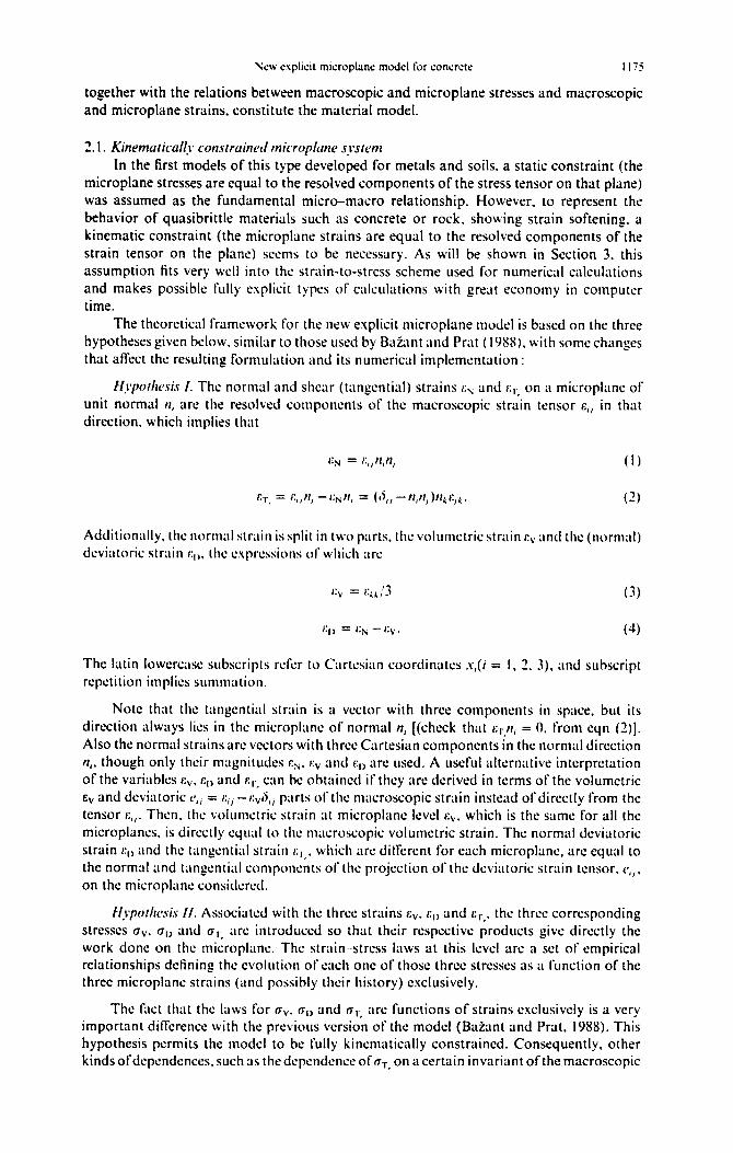
which correspond to a prescribed value of macroscopic strains [see the scheme in Fig. (I)] : from the macroscopic strain increment, the microplane strain incrcmcnts are evaluated by

using cqns (l)-(4) then the microplane stresses are computed using the stress-strain laws

dcfincd at the microlcvel, and finally the new macroscopic stress tensor is obtained by

integration of microplane stresses according to eqn (5).

MACROSCOPIC MICROPLANE

LEVEL LEVEL

STRAIN Eii

I KilWlll~liC

(INPUT DATA.) conctraint ‘- G #ED ,ETr

I

1

Microplanr laws -

STRESS ai principle of

(OUTPUT Virtual Work av ,a0 ,Gr

RESULT 1 I

Fig. I. Basic scheme for the computation of macroscopic stresses rrom the macroscopic strains.

1176 I. CAROL el ul.

stress tensor assumed in previous works (which in fact established a "mixed" kinematic­static constraint for the model) are in this case excluded from the formulation.

Hypothesis III. The relationship between the microplane stresses (fv. (fo and aT, and the macroscopic stress tensor ai, is obtained by applying the principle of virtual work. Its application to this case is explained in some detail in Appendix A. including certain considerations about symmetry requirements for the tensors 0',/ and c'l necessary to ensure interchangeability of the indices i and j in the final expressions (the symmetry considerations used in the Appendix are an alternative to the a priori symmetrization of eqn (2) used in previous works to reach the same final effect). The expression for the macroscopic stress is then:

(5)

where the integral domain represented by n represents the upper half hemisphere and (j;i

is the Kronecker delta.

An important new feature of eqn (5) is that it is written in terms of the total values of stresses instead of differential increments. The equation would also be valid if all the stress variables were replaced by their differential increments. which was how it was presented in the original formulation (Bazant and Prato 1988). If. however. the equation is written in terms of the total values. then the current (total) value of the macroscopic stress tensor "'i

can be obtained from the current (total) values of the microplane stresses "v. ITp and ITI, at any moment during the load history. by direct application of eqn 5. This desirable feature cannot be obtained from the incremental-type equation.

Another advantageous 'Ispect of eqn (5) is that is permits a clear interpretation of the contribution of each of the microplane stresses ("v. "D and "I) to the macroscopic stress tensor ",/. From that equation. one can see that the "v term gives a volumetric contribution to ",/. and the "I, term gives a pure deviatoric contribution to the macroscopic stress tensor (this becomes clear by noting that this term becomes zero if i = j). The ITIl term is the only one which gives both volumetric and deviatoric contributions to the macroscopic stress tensor. Consequently. this term is responsible for the intrinsic coupling the model shows between volumetric and deviatoric behavior. such as deviatoric-induced dilatancy. etc.

With the three hypotheses presented. and provided that specific definition of the microplane stress-strain relationships is given according to Hypothesis II. the basic frame­work of the model is complete and it is already possible to calculate the macroscopic stresses which correspond to a prescribed value of macroscopic strains [see the scheme in Fig. (I)] : from the macroscopic strain inerement, the microplane strain increments are evaluated by using eqns (1)-(4) then the microplane stresses are computed using the stress-strain laws deli ned at the microlevel, and finally the new macroscopic stress tensor is obtained by integration of microplane stresses according to eqn (5).

MACROSCOPIC MICROPLANE LEVEL LEVEL

STRAIN Eli Kln.matic Ev ,ED ,ETr ..

(INPUT DATA) con_traint

J ! Mieraplan ..

prinCiPI} of

laws -

STRESS all .. Ov 'aD ,0Tr (OUTPUT Virtual Wor. RESULT) I

Fig. I. Basic scheme ror the computation or macroscopic stresses from the macroscopic strains.

New explicit microplane modsl for concrrtr 11’7

Although not always necessary, in certain situations (e.g. as a part of a FL program).

it is useful to calculate additionafly the macroscopic tangential stiffness tensor Diik,. relating

macroscopic stress and strain increments. In particular. this tensor is required to obtain the

tangential stiffness matrix of the structure whose eigenvalues decide path bifurcations and

determine the stable paths (Baiant. 1988 ; de Borst. 1987). The expressions for D,,II can be

easily derived from the incremental counterpart ofeqn (5) by substituting for the microplane

stresses their expressions in terms of microplane strains and then, for the microplane strains

their expressions in terms of the macroscopic strains. However. since the resulting stiffness

expression can be different depending on the type of stress-strain laws used at microplane

level, this derivation will be given in Section 2.4, after the definition of the microplane IUNS.

Within the basic framework presented. a very wide range of models can still be defined

depending on how the microplane stress-strain relationships are chosen. In this work. the

laws for bv, on and or, have been selected on the basis of those used in previous versions

of the microplane model (Baiant and Pmt. 1988) but with some modihcations and new

dependencies so as to make numerical implementation more convenient.

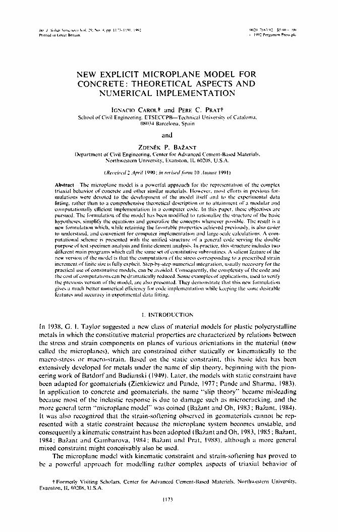
(a) E’oltirnttri~ km. This microplane lr~w dircctIy reproduces the macroscopic behavior

of the material when only volumetric strains or stresses are present. Thcrcforo. a curve that

tits cxpcrimcntal data for hydrostatic tests may be directly introduced. For compression

(av > 0) the following law is i1SSlUllCd :

while for hydrostatic tension (av < 0)

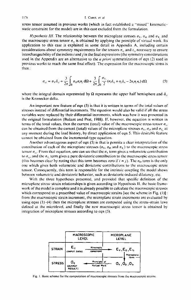
whsrc Et, 11, h, p, (1. u,, 11, arc empirical material constants obtain4 by titting a single cxpcrimcnt:rl curve. The volumetric law is plotted in Fib 1. 21. For unloading--rclonding, both the tcnsilc and compressive curves act as envelopes. In compression the unloading branches

are assumed to always have the initial slope E z, and the origin of the tcnsilc part of the diagram always shifts to the point in which the unloading compressive branch rcachcs the

horizontal axis. The unloading-reloading in tension is assumed to follow a sCWnt slope

bctwccn the maximum point reached in the tensile curve and the origin of that curve.

(b) ~V{~r~rl~~f ~l~~~irr~t~rj~ hs. This law is based on the same type of cxp~n~Iiti~ll stress-

strain envelope curve used for the tensile part of the volumetric behavior, but now con-

sidering two ditferent sets of parameters for tension and compression

where Ei. a,. p,, u2. pz are empirical material constants, The law is rcprcscnted in Fig. 2b.

For unloading-reloading. straight lines arc assumed with a certain slope. For compressive behavior the initial slope EE is always used, while a secant slope (from the origin to the

point of maximum positive strain previously reached} is used on the tensile side of the

diagram. For unloading in compression, the origin of the tensile pnrt of the diagram is always assumed to shift to the point in which the unloading compressive branch intersects the horizontal axis.

New explicit microplane mode:! ror concrete: 11'7

Although not always necessary. in certain situations (e.g. as a part of a F.E. program). it is useful to calculate additionally the macroscopic tangential stiffness tensor Dllkl • relating macroscopic stress and strain increments. In particular. this tensor is required to obtain the tangential stiffness matrix of the structure whose eigenvalues decide path bifurcations and determine the stable paths (Bazant. 1988; de Borst. 1987). The expressions for DII" can be easily derived from the incremental counterpart of eqn (5) by substituting for the microplane stresses their expressions in terms of microplane strains and then. for the microplane strains their expressions in terms of the macroscopic strains. However. since the resulting stitTness expression can be different depending on the type of stress-strain laws used at micro plane level. this derivation will be given in Section 2.4. after the definition of the microplane laws.

2.2. COllstilUtice relationships used at the microplCllle terel Within the basic framework presented. a very wide range of models can still be defined

depending on how the microplane stress-strain relationships are chosen. In this work. the laws for UY. Un and UT, have been selected on the basis of those used in previous versions of the microplane model (Ba:z.mt and Prato 1988) but with some modifications and new dependencies so as to make numerical implementation more convenient.

(a) Volumetric law. This microplane law directly reproduces the macroscopic behavior of the material when only volumetric stmins or stresses are present. Therefore. a curve that fits experiment .. 1 data for hydrostatic tests m~ly be directly introduced. For compression (lTy > 0) the following law is assumed:

(6)

while for hydrostatic tension (lTy < 0)

(7)

where £~. tI. h. p. tJ. tI,. 1', are empirical material constants obt~lincd by fitling a single experimental curve. The volumetric law is plotted in Fig. 241. For unloading--rcloading. both the tensile and compressive curves act as envelopes. In compression the unloading bmnches arc assumed to always have the initial slope E~. and the origin of the tcnsile part or the diagram ,llways shifts to the point in which the unloading compressive branch reaches the horizontal axis. The unlouding-rcloading in tension is assumed to follow a secant slope between the maximum point reached in the tensile curve and the origin of that curve.

(b) Normal del'ialOric fall'. This law is based on the same type of exponential stress-­strain envelope curve used for the tensile part of the volumetric behavior. but now con­sidering two different sets of parameters for tension and compression

(8)

(9)

where Eg. a,. PI' a~. p~ are empirical material constants. The law is represented in Fig. 2h. For unloading-reloading. straight lines arc assumed with a certain slope. For compressive behavior the initial slope Eg is always used. while a secant slope (from the origin to the point of maximum positive strain previously reached) is used on the tensile side of the diagram. For unloading in compression. the origin of the tensile part of the diagram is always assumed to shift to the point in which the unloading compressive branch intersects the horizontal axis.

1. CAKl)L Y1 d

a)Volumetrlc stress-strarn relatlonshlp

b) Normal dewatoric stress-stram relatlonshm

c)Tangent~al stress-strain madulc relatlonshlp

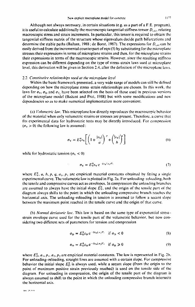
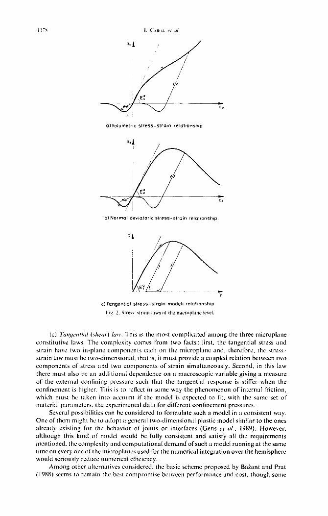
I:ig. 2. Strczs str;tirl I;iws ;It tIi~ microplaw lovcl.

(c) 7irr~,qc~r/itr/ (slk~r) /UW. This is the most complicated among the Lhrcc niicroplanc

constitutivc laws. The complexity comes from two facts : first. the tangcntiul stress illld

strain h:lvc two in-plant components t!i\ch on the microplanc and. thcrcforc, the stress

strain law must lx two-dimcnsionul, that is, it must provide it coupled relation bctwccn two

components of stress itnd two components of strain simultnncously. Second. in this law

thcrc must also bc an additional dcpcndcncc 011 il macroscopic v:tri;~blc giving ii measure

of the c.ytcrn;lI conlining prcssurc such that the tangential rcsponsc is stilrcr when the

contincmcnt is hi&r. This is to rcllcct in sonic way the phcnomcnon of internal friction.

which must bc taken into account it’ the model is cxpcctcd to lit. with the same set 01 material paramctcrs. the cspcrimcntal data li)r dillkrcnt confincnicnt prcssurcs.

Scvcr:ll possibilities can bc considcrcd to Ibrmulatc such iI model in ;I consistent way.

One of them might bc to adopt ;I gcncral t~vo-tliln~nsion;lI plastic model similar to the ones already existing ror the bchilvior of joints or intcrfnces (Gas CI (I/.. 1989). However,

illthough this kind of model would bc I’ully consistent and satisfy all the rcquircmcnts mcntioncd. the complexity ilnd computiltionill domand’of such iI model running at the same time on cvcry one of’thc microplancs used for the numerical integration over the hemisphcrc would seriously rcducc nunicrical cf~iciency.

Among other altcrnativcs considcrcd. the basic schcmc proposed by Baiant and Prat (19S8) seems to remain the btst compromise bctwccn performance and cost, though sonic

117S I. CAIWL ~I 1.1i.

.' ' , I

a) Volumetric stress -strain relationship

---:+~,----,I-----------­

b) Normal deviatoric stress-strain relationship.

C) Tangential stress - strain moduli relat lonshi p

hg. 2. Sln:ss slrain laws at th.: mi.:roplan.: kvd.

E.

(l:) Tal/gel/tia/ (.I'/iear) /all'. This is the most complicated among the three mil:roplane constitutive laws. The complexity l:Ol11es from two f:ll:tS: first. the tangential stress and strain have two in-plane l:omponents eadl on the mil:roplane and. therefore. the stress· strain law must be two-dimension.ll. that is. it must provide a coupled relation between two l:omponents of stress and two wmponents of strain simultaneously. Sewnd. in this law there must also be an additional dependelKe on a mal:rosl:opil: variable giving a measure of the external confining pressure SUdl that the tangential response is stiller when the confinement is higher. This is to relled in some way the phenomenon of internal fridion. whil:h must be taken into al:l:ount if the model is expel:ted to fit, with the same set of material parameters. the experiment.tI d.lta for dillerent l:onfinel11ent pressures.

Several possibilities l:an be l:onsidered to formulute sUl:h a model in a l:onsistent way. One of them might be to adopt a general two-dimensional plastic model similar to the ones already existing for the behavior of joints or interl:lces (Gens £'1 a/ .• 1989). However. although this kind of model would be fully wnsistent and satisfy all the requirements mentioned. the complexity and l:omputational demand' ofsueh a model running at the same time on everyone of the mil:roplanes used for the numerical integration over the hemisphere would seriously reduce numeril:al elliciency.

Among other alternatives considered. the basic scheme proposed by Bazant and Prat (1988) seems to remain the best compromise between perrormance and cost. though some

SW r.kphcir microplait: modd for wncrctr 1170

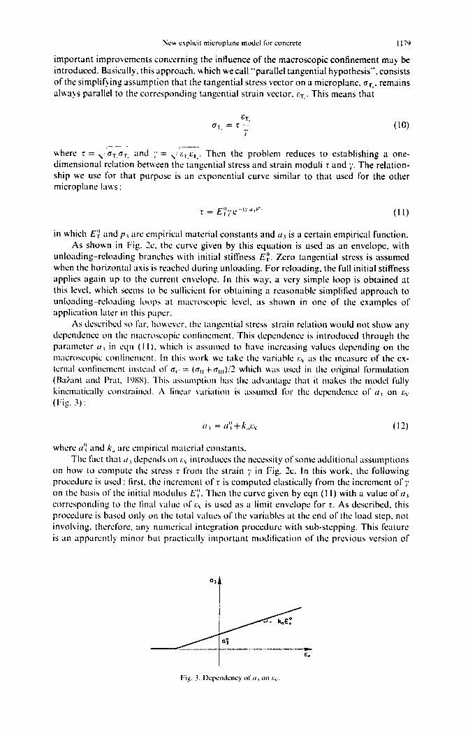
important improvements concernin g the intluence of the macroscopic confinement may be

introduced. Basically. this approach, which we call “parallel tangential hypothesis”. consists

of the simplifying assumption that the tangential stress vector on a microplane. or,, remains

ahva\s parallel to the corresponding tangential strain vector. Er,. This means that

Err ‘T, ., ET--

I

where r = \ ‘GGy illld ;’ = bIcCiI. Then the problem reduces to establishing a one-

dimensional relation between the tangentiul stress and strain moduli T and 7. The relation-

ship ~‘e use for that purpose is an exponential curve similar to that used for the other microplime la\vs :

in which E’: and p, are empirical m;~teri:ll constants and (li is ;L certain empirical function.

As shown in Fig. 2c. the curve given by this equation is used as an envelope. with

unloading-reloading branchcs with initial stiffness E” r. Zero tangential stress is assumed

when the horizontal axis is reached during unloading. For reloading the full initial stifTness

applies again up to the current envelope. In this way. ;I very simple loop is obtained at

this Icvcl. which seems to be sulticicnt for obtaining n reilsonablc simplified approach to

unloaJing-rclo~ldirlg lo~~ps at macroscopic Icvel, as shown in one of the examples of

application IiltCr in this paper.

AS dcscribcd so far. howcvcr. the tilngcntiill stress strain relation would not show any

dcpcndcncc on the macroscopic conlincnicnt. This tlcpcndcncc is inlrotluccd through the

paramctcr (I, in eqn ( I I ). which is assumctl to have increasing valucS dcpcnding on the

m;lcroscopic conlincrncnt. In this work WC take the vuriahlc ~:v ilS the measure of the cx-

turnal conlincmcnt instcacl of ~7~. = (f~,, + rr,,,)/7 which WilS usctl in the 0rigiIlill formulation

(fkliit~~t ilntl I’rat. I’M). This assumption has the ;ltlv:mt:lgc that it ~n:~kc~ Lhc m~dcl fully

kincni:ilically constrained. A linear varkition is assunicrl for lhc dcpcntlcncc of (I, on 1:” (I:ig. 3) :

(I, = (1’; + IQ, (1’)

whcrc (1’: illd k,, iIK elnpirkill rwtcriiil WIlStilnlS.

The fact that II, tlcpcntls on I:\ introduces the ncccssity of some :~cltlitional assumptions

on how to compute the stress T from the strain ;’ in Fig . 2~. In this work. the following

proccdurc is used : lirst, the incrcmcnl of T is computed cI:ISticidIy from the incrcmcnl of;

on the basis of the initial modulus f?,‘. Then the curve given by cqn (I I) with ;L value oft,

corresponding to the limil v~iluc of I :\ is IISL’~ ilS il limit cnvclop~ for T. AS described, this

proccdurc is bused only on the tot;11 \~illucs of’tk vnriublcs at the end of the load step. not involving. thcrcforc, any numerical integration proccdurc with sub-stepping. This feature

is iln apparently minor but prilctically important modilication of lhc previous version of

:\cw c.\pllcit microplanc modd for concn:tc: 1[79

important improvements concerning the influence of the macroscopic confinement may be introduced. Basically. this approach. which we call "parallel tangential hypothesis", consists of the simplifying assumption that the tangential stress vector on a microplane, Ufo' remains always parallel to the corresponding tangential strain vector. f.r.' This means that

( 10)

, r---'-where r = ,,' ar.ar, and :. = .. ,/f:r.Cr .. Then the problem reduces to establishing a one-dimensional relation between the tangential stress and strain moduli r and i'. The relation­ship we use for that purpose is an exponential curve similar to that used for the other microplane laws:

( II )

in which E~ and (I, are empirical material constants and £I., is a certain empirical function. As shown in Fig. 2c. the curve given by this equation is used as an envelope. with

unloading-reloading branches with initial stitfness £~. Zero tangential stress is assumed when the horizontal axis is reached during unloading. For reloading. the full initial stilrness applies again up to the current envelope. In this way. a very simple loop is obtained at this level. which seems to be sullicient for obtaining a reasonable simplified approach to unloading-reloading IO\lps at macroscopic level. as shown in one of the examples of application later in this paper.

As described so rar. however. the tangential stress strain relation would not show any dependence on the m;Icroscopie conlinement. This dependence is introduced through the parameter tI, in et(n (II). which is assumed to have increasing values depending on the macroscopic c(ltliinelllent. In this work we take the varianle 1:\ as the measure of the ex­ternal conlinement instead of (Tc = «(Til + (T1II)/1 which was used in the original rormulation (Baiant and Prato 191'1'). This assumption has the advantage that it makes the model fully kinematically constrained. A linear variation is assullled for the depcndence or (/, on 1:\

(Fig. J):

( 11)

where tI': and k" are empirical material constants. The fact that tI, depends on 1:\ introduces the necessity of some additional assumptions

on how to compute the stress r rrom the strain i' in Fig. 1c. In this work. the following procedure is used: first. the increment of r is computed elastically from the increment or i' on the basis of the initial modulus £;'. Then the curve given by eqn (II) with a value of a.1 corresponding to the linal value of 1:\ is used as a limit envelope for r. As described. this procedure is based only on the total values of the variables at the end of the load step. not involving. therd"ore. any numerical integration procedure with sub-stepping. This feature is an apparently minor but practically important modification of the previous version of

------~------~---------------~ E.

Fig. 3. J)cpclllIcncy Ill' (/, I1n I:\".

I IN) 1. C\KOL 1’1 01

the model (in which the numerical integration procedure was needed) : it makes possible a

fully explicit computation of a strain-prescribed load step. which is one of the objectives of

this work.

2.3. Purh-~i~~rtrrit~n~~t~ As is clear from eqns (6)-( II!). the microplane stress-strain relations are total-strain

relations which are path-independent for the case of monotonic loading on the microplane.

It is important to note. however. that the macroscopic response for macroscopically mono-

tonic loadins is path-dependent. The reason is that even such loading normally involves

unloading (for volumetric or deviatoric curves) or change of direction (for shear) on some

microplanes. As in the previous microplane model. it is assumed that all the macroscopic

path-dependence stems from the possibility of various combinations of loading and unload-

ing on the microplanes.

This is an attractive simplifying theoretical feature of the rnodcl. In practice. however.

some numerical precautions must be taken due to the numerical scheme used. explained in

Section 3. According to the kinematic micro-macro constraint assumed. the change of

direction of the microplane strains must come from ;I change in direction of the macroscopic

strains. As will be shown in Section 3. the increments of strains. stresses and other variables

arc calculated for each loild step within ;I loop over the number of external loi\tl steps. In

the (macroscopic) strain space. the strain increment corresponding to ;I load step is rcp-

resented by ;i straight scgmcnt. and the segments of the subsqiicnt load steps constitute il

poly~onnl approximation to the true strain pilth. In gcncrnl. the trut strain pilth ivill bc ;l

curve not necessarily smooth (t2.g. consider the sudden dcvclopmcnt of IiltlXll dilatancy in

;I uniarial test ncilr the peak. as in the first cxamplc prcscntcd in Section 4). C’onsqucntly,

it is clcnr that in practice the load history must hc divided into ;I suliicicnt nunihcr of load

steps so that the true strain path and. thcrcforc. the corresponding loading unloading

combinations in the microplilncs. can bc capturccl in the n~lculations.

2.4. ‘liutqcwl ttrtri~rosc~o~tic. sIij]kw Icwsor

I:or the derivation ol’thc macroscopic tangent stili‘ncss matrix. cqn (5) must bc rcwriltcn

in lcrnis of the tlilYcrcnti;il stress incrcnicnts instead of the total values:

df7,, = da,&, + 3

s 3n fl dd,,/l,tl, dR + ‘-

s

da,

271 <) 2 c (tt,d,, +,I,&, -2tt,tt,tt,)dQ. (13)

Then the incrcmcnts ofstresses iit the microplane lcvcl must be replaced by their incrcmcntaI

expressions in terms of the current tangent modulus and the incrcmcnts of strain at that

Icvel. Thcsc are simple scalar expressions for da, and dn,,,

but not for drr,., sincc both the tangential stress and strain on it microplanc arc vectors.

Their incromcntal relationship must involve it matrix :

da,, = C/l:” dr:,<. (16)

The matrix Ii:‘:” for the parallel tangential model used in this work is derived in

Appendix IX Its final expression involving the tangential shear stiffness E’;‘” (obtained from

the relationship ds = Ey”dy) ils well Ils the current values of ‘T~,,E~, and their rcspcctivc moduli r and ;‘. is

111'0 I. C'JWL el 1.11.

the model (in which the numerical integration procedure was needed) : it makes possible a fully explicit computation of a strain-prescribed load step. which is one of the objectives of this work.

2.3. Path-dept'l/dt'nce

As is clear from eqns (6)-( 12). the microplane stress-strain relations are total-strain relations which are path-independent for the case of monotonic loading on the microplane. It is important to note. however. that the macroscopic response for macroscopically mono­tonic loading is path-dependent. The reason is that even such loading normally involves unloading (for volumetric or deviatoric curves) or change of direction (for shear) on some microplanes. As in the previous microplane model. it is assumed that all the macroscopic path-dependence stems from the possibility of various combinations of loading and unload­ing on the microplanes.

This is an attractive simplifying theoretical feature of the modd. In practice. however. some numerical precautions must be taken due to the numerical scheme used. explained in Section J. According to the kinematic micro-macro constraint assumed. the change of direction of the microplane strains must come from a change in direction of the macroscopic strains. As will be shown in Section J. the increments of strains. stresses and other variables arc calculated for each load step within a loop over the number of external load steps. In the (macroscopic) strain space. the strain increment corresponding to a load step is rep­resented oy a straight segment. and the segments of the suosequent load steps constitute a polygonal approximation to the true strain path. In general. the true strain path will be a curve not necessarily smooth (e.g. consider the sudden dcvdopnh.:nt of lateral dilatancy in a uniaxial test near the peak. as in the first example presented in Sel·tion 4). Consequently. it is clear that in practice the load history must be divided into a suflicient number of load steps so that the true strain path and. therefore. the corresponding loading unloading combinations in the microplanes. can be captured in the calculations.

2.4. Ttil/gellt I/UlcrosClipic stijJiles.\" t('I/SlIr

For the derivation of the macroscopic tangent stifi"m;ss matrix. eqn (5) must he rewritten in terms of the difl"crential stress increments instead of the total values:

(I J)

Then the increments of stresses at the microplane kvd must be replaced by their incremental expressions in terms of the current tangent modulus and the inerements of strain at that kvel. These arc simple scalar expressions for dl1v and dl1 J).

( l-l)

( 15)

but not for dl1l', since both the tangential stress and strain on a microplane are vectors. Their incremental relationship must involve a matrix:

( 16)

The matrix fI~·:n for the parallel tangential model used in this work is derived in Appendix B. Its final expression involving the tangential shear stiffness £Ij-'" (obtained from the relationship dr = £'['" di') as well as the current values of I1T • f.r and their respective moduli r and ~'. is ' ,

NW explicit micropbr model for concrete 1181

(17)

Introducing eyns (l-t)-( 16) into eqn (13) and then replacing the microplane strain

increments according to eqns (Z)-(4). the final expression of the tangent macroscopic

stilfness matrix D$, can be obtained. This derivation is presented in Appendix C and it

requires the introduction of certain symmetry considerations for identifying the matrix

coefficients from the resulting equation (or alternatively. the use of an apriori symmetrized

version of eqn (2). as done in previous works) in order to pet a stiffness expression that

satisties the interchangeability of stress tensor indices i and j and the strain tensor indices

k and 1. The final expression is :

da,, = D I::, dEk, (18)

where

Nutc that this is not the same cxprcssion as obtained by Baiant and Prat (1988). whcrc

the rckltionship bctwocn macroscopic strain and stress incrcmcnts was dcr,, = C,,,, dr:k,+da;‘,

with the additional initial slross term ; the tensor C,,,,did not have the meaning of tangential sti tl’ncss.

Prior to establishing the linnl list of model paramctsrs. it is useful to relate the three

initial moduli of the microplanc stress strain laws El). L+i: and EF. which do not have any

macroscopic physic;lI mcnning. to the standard elastic paramctcrs. This can bc easily

achicvcd if WC impost the condition that virgin concrctc initially follows a lincar elastic

bchahior. In that situation the behavior on any microplanc is the same: linear elastic

functions for rrv. r~,, and 6, in terms of their respective strains with initial moduli Et. EL

;llld El'. Thcsc cquiltions can bc introducsd into the intsgral in .eqn (5). the microplane

strains rcplaccd according to crlns (Z)-(4). and the integral over the hcmisphrre solved by

hand, from which ;I tinal linear relationship bctwcrn macroscopic stress and strain is

obtained. 11~ identifying the coclticicnts of that cxprcssion with the cocllkients of Lamb’s

equation of elasticity, the following relations arc obtained (13aZant and Prat. 1988) :

E” = 1 50-~~) I

11

_. _.. _ 3 ‘I+\*

2#lo I?;. 1 (22)

Thus. Young’s modulus. E. Poisson’s ratio. 1’. and the additional parameter. q,,, can be

used as input parameters instead of the three initial moduli at microplane level. Then the

program calculates the values of those moduli internally.

The final list includes a total of I4 parameters :

(i)---Elastic paramctcrs: E, \* and ‘1”.

(ii&Volumetric law: (1. h. p, q. a, and p,.

~ew ex.plil:it mil:roplane model for wnl:rete Illll

(17)

Introducing eqns (14)-(16) into eqn (\3) and then replacing the microplane strain increments according to eqns (2)-(4). the final expression of the tangent macroscopic stillness matrix D~~::, can be obtained. This derivation is presented in Appendix C and it requires the introduction of certain symmetry considerations for identifying the matrix coefficients from the resulting eq uation (or alternatively. the use of an a priori symmetrized version of eqn (2). as done in previous works) in order to get a stiffness expression that satisfies the interchangeability of stress tensor indices i and j and the strain tensor indices k and I. The final expression is:

( 18)

where

( 19)

;\;ote that this is not the same expression as obtained by Bazant and Prat (1988). where the rdationship between mal:rosl:opic strain and stress im:rements was dU'1 = C"., dl:k1 + dU;'i with the additional initial stress term; the tensor Cil ., did not have the meaning of tangential stilrness.

2.5 .. \·/11l/lllary or thc lIIodclparamcters alld their !'alliL's Prior to est~lblishing the linal list of modd parameters. it is useful to relate the three

initial moduli of the ll1il:ropl~\Ile stress stmin laws E~. E:~ and E~. whil:h do not have any l11al:roswpil: physil:al meaning. to the standard clastic parameters. This can be easily achieved if we impose the I:ondition that virgin I:onl:rete initially follows a linear elastic behavior. In that situation the behavior on any mil:roplane is the same: linear clastil: funl:tions for ([v. ([u and ([, in terms of their respective strains with initial moduli E~. E~ ~lnd E~. These equations I:an be introduced into the integral ineqn (5). the microplane strains replal:ed al:cording to eqns (2)-(4). and the integral over the hemisphere solved by hand, from whil:h a linal linear relationship between mal:roscopie stress and strain is obtained. By identifying the I:oellkients of that expression with the coetneients of Lame's equation of elastil:ity. the following relations arc obtained (Bazant and Prato 1988):

(J E Ev = ---------1-2\'

(20)

(21)

(22)

Thus. Young's modulus. E. Poisson's ratio. \', and the additional parameter. '10. can be used as input parameters instead of the three initial moduli at microplane level. Then the progr~lm calculates the values of those moduli internally.

The final list includes a total of 14 parameters:

(i)-EI'lstic parameters: E. \' and '10' (ii)-Volumetric law: (/. h.p. q. ", and 1',.

IIS? I. C\HOL <‘I ui.

(iii)--Normal deviatoric law : u2 and p:

(iv)-Tangential law : a’,‘. k, and p:.

However, the six volumetric law parameters can be identified separately by simple curve

tittinp of the compressive and tensile hydrostatic stress-strain curves. Of these six

parameters. five can be usually assumed to have the same values for most concretes:

0 = 0.OOS.h = 0.3.p = 0.25.q = 2.25.p, = o.s.co nstants Eand v are knotvn from elastic

tests. Thus. only seven parameters need to be identified by fittinp other than hydrostatic test

data on the basis of eyn (6). Furthermore. experience shoivs that for most concretes. one

can use pz = p, = 1.5. Consequently. there are only five parameters. q,,. u,. N:. (I!; and k,,. which must be determined to fit the esperimental data for non-linear triaxinl behavior

curves. Moreover. in the case of tats with ncgligiblc confining pressure. h-,, = 0 can be used

and the number of p;lr;lmetcrs is reduced to only four. With only five or four unknolvn

parameters. the titting of non-linear triaxial test data is not ditticult.

3. SUMERICAL IMPLEMENTATION

We now present ;i uni tied scheme for two computer programs serving the purposes of

both “single-point” constitutive vcritication and F.E. structural analysis. This schcmc

involves t\vo (constitutivc) niodcl-indcpcndclit main prosrams and one (constitutive)

model-specific set of subroutines.

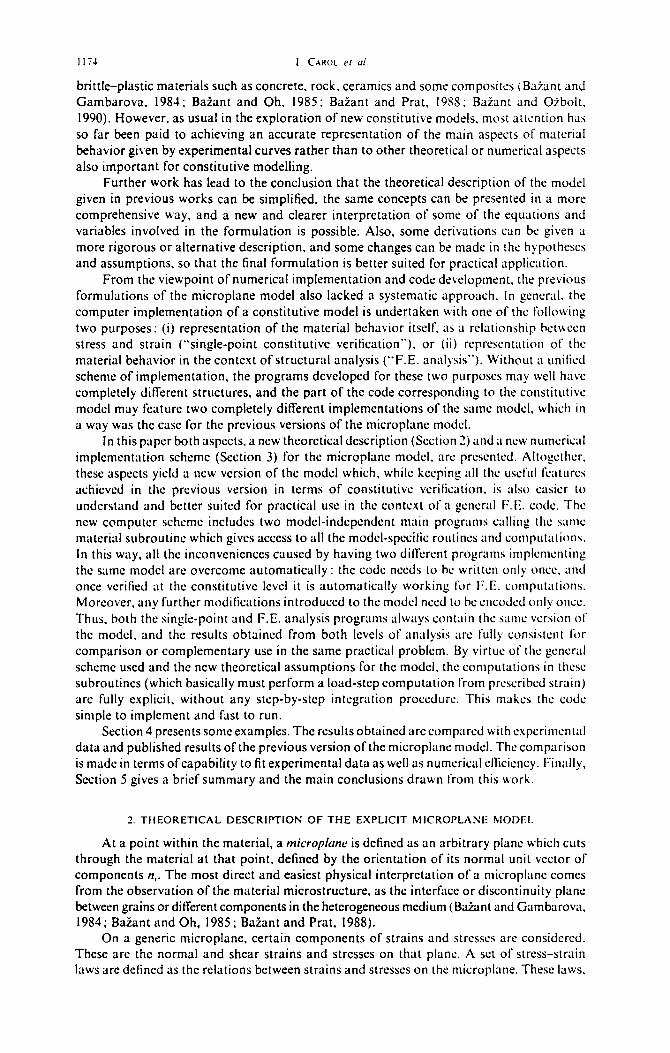
Figure 41 shows the basic llo&hart of the “single-&int” main program dcvclopctl for

constitutivc vcritication , and Fig. 4b the s;inic schcmc for the companion F.E. main

program. fIoth diapr~inis prcscnt ;I similar structure, though the l:.I:,. program obviously

inclutlcs all the xldition;iI 0pcr;itions for calculatin, 4~ clcnicnt still’ncss matrices. etc. After

the gcncral tl;~t;~ input, ;I first loop over the number of load steps can bc obscrvcd in both

programs. f:c>r the linitc clcnicnt progr:im . ;I load step consists . as usunl, of ;i set of npplicd lo;~rls and prcscrihcd nodal displaccnicnts, while for the sin+point program ;I load step

consists of ;I set of values ol’cithcr prcscrihctl stress or prcscribcd strain for cnch of the six

dcgrccs of frccrloni considcrcd at the constitulivc Icvcl.

In both programs. the non-linear analysis of each load step is carried out by using ;I

standard itcrativc initial-stress type strategy. This is rcllcctccl in the Ilowchnrts with the

inner loop controlled by an IF statcmont at the bottom of the diagrams. As II consequence

of using the same non-linear strategy, the s;tmc type of constitutivc computntions arc

rcquirccl for an iteration in both programs. Those computations arc of the prcscribcd strain

type, i.e. knowing the previous (initial) state and the v;~lucs ofu prcscribcd strain increment,

the new linal state (including the new values ofstrcsscs) must bc obtained.

Note that the sin&z-point main program of Fig. 41 deals directly with the components of strain and stress at ;I point of the m;ltcrial. In gcncctl. similar results can bc obklinctl

usincy c ;I finite clcmcnt program \vith ;I single clomcnt. Howcvcr, thcrc may bc ditkrcnccs

bctwccn the two types of analysis when stress (and not only strain) is prcscribcd to some

of the dcgrccs of frcctlom. Then. if uncspcctcrl results arc to bc intcrprctcd. it bccomcs

dillicult to distinguish H.hcthcr they arc due to the constituti~~c nioclcl itself or to spurious or non-spurious but uncapcctcd behavior of the linitc clcmcnts (it is possible to obtain

apparently correct but misleading results from I:.E. computations with one or few clcmcnts. since the method is cxpcctcd to convcrgc to the solution of the physical problem studied

only when the mesh is tint enough).

The unified implcmcntation of the computational schcmcs for constitutivc verification

and for F.E. analysis. has important advantqcs which in gcncral arc clear to the specialists on large-scnlc computer programming. but stem to bc unapprcciatcd by many solid mech- anicists who spccializc in material modclling. One obvious advantage of the unified schcmc presented hcrc is that n sin@ subroutine (or set of subroutines) for the constitutive model

needs to bc dcvclopcd for both Icvcls of analysis. This subroutine (or set of subroutines) can be dcbuggcd and testcd with the single-point main pro_cram . and then. after this phase

I. C \I{()l ('( U/.

(iii)-Normal deviatoric law: a: and P:­(iv)-Tangential law : ali. k" and p,.

However. the six volumetric law parameters can be identitied separately by simple curve fitting of the compressive and tensile hydrostatic stress-strain curves. Of these six parameters. five can be usually assumed to have the same values for most concretes: {i = 0.005. h = 0.225.p = 0.25. q = 2.25,p, = 0.5. Constants Eand \' are known from elastic tests. Thus. only seven parameters need to be identified by fitting other than hydrostatic test data on the basis of eqn (6). Furthermore. experience shows that for most concretes. one can use P: = PI = 1.5. Consequently. there are only five parameters. '1". (/1' {i> ali and k". which must be determined to fit the experimental data for non-linear triaxial behavior curves. Moreover. in the case l)f tests with negligible contining pressure. k" = 0 can be used and the number of parameters is reduced to only four. \Vith only five or four unknown parameters. the titting of non-linear triaxial test data is not ditlicult.

J. SUMERICAL l~lPLEMENTt\T10N

We now present a unitied scheme for two computer programs serving the purposes of both "single-point" constitutive veritication and F.E. structural 'lI1alysis. This scheme involves two (constitutive) model-independent malll programs and one (constitutive) model-specilic set of subroutines.

3.1. Fiml'c/r(/rIS jill' c(llISlillllicc raiji('(/li(ll/ tll/t! F. E (/I/(/Iysis

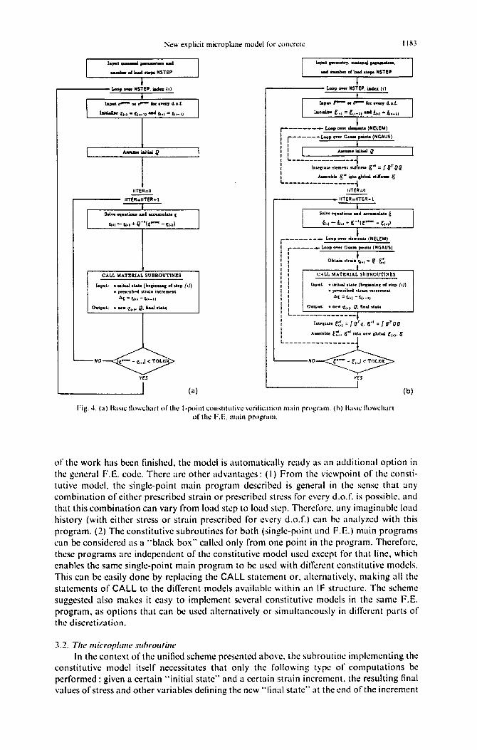
Figun: 4a shows the oasic tlowchart of the "single-point" main program developed for constitutive verilication. and Fig. 40 the same scheme for the companion F.E. main program. Both diagrams present a similar structure. though the F.E. program ooviously includes all the additional operations for cakulating element stilrness matrices. etc. After the general data input. a lirst loop over the nlllllbn of load steps can be observed in both programs. For the tinite element program. a load step consists. as lIsual. of a set of applied loads and prescrioed nodal displacements. while for the single-point program a load step consists of a set of values of either prescribed stress or prescribed strain for each of the six degrees of freedom considen:d at the constitutive level.

In both programs. the non-linear analysis of each load step is carried out by using a standard iterative initial-stress type strategy. This is rclkcted in the Ilowcharts with the inner loop controlled by an IF statement at the bottom of the diagrams. As a consequence of using the same non-linear strategy. the same type of constitutive computations arc required for an iteration in both programs. Those computations arc of the prescribed strain type. i.e. knowing the previous !initial) state and the values of a prescribed strain increment. the new final st'lte (including the new values of stresses) must be obtained.

Note that the singk-point main program of Fig. 4a deals directly with the components of strain and stress at a point of the material. In general. similar results can be obtained using a finite clement program with a single clement. However. there may be ditl'crences between the two types of analysis when stress (and not only strain) is prescribed to some of the degrees of freedom. Then. if unexpected results are to be interpreted. it bel:omes dillicult to distinguish whether they arc due to the constitutive model itself or to spurious or non-spurious but unexpected behavior 01" the tinite clements (it is possible to obtain apparently correct but misleading results from F.E. computations with one or few elements. since the method is expected to convcrge to the solution of the physical problem studied only when the mesh is line enough).

The unified implementation of the comput.ltional scllemes for constitutive verification and for F.E. analysis. has important advantages which in general arc clear to the specialists on large-scale computer programming. but seem to bc unappreciated by many solid mech­anil:ists who spel:ializl: in material modelling. One obvious advantage of the unified scheme presented here is that a single subroutine (or set of subroutines) for the constitutive model needs to be developed for both levels of analysis. This subroutine (or set of subroutines) can be debugged and tested with the single-point main program. and then. after this phasc

I (4 (b)

of the work hiIs been finished. the model is ~tutomatic:llly reildy 3s an itdditionill option in

the gcncrul F.E. code. There arc other advi~nt:~ges: (I) From the viewpoint of the consti-

tutive model, the single-point main program described is general in the sense that any

combination ofeither prcscribcd strain or prescribed stress for every d.o.f. is possible. und

that this combination can vary from load step to loud step. Thcrcforc. any imaginable load

history (with either stress or strnin prescribed for every d.o.f.) can be iIn:ilyzed with this

program. (2) The constitutivc subroutines for both (single-point and F.E.) main progrnms

can be considered ;Is 3 “bliick box” called only from one point in the program. Therefore,

these programs arc indcpendcnt of the constitutive model used except for that lint. which

enables the same singlepoint main program to bc used with different constitutivc models.

This can be easily done by replacing the CALL statement or, altcrnativcly. making all the

statements of CALL to the different models nvililuble uithin an IF structure. The schcmc

suggested also makes it easy to implement sevcritl constitutivc models in the same F.E.

program. as options that can be used alternatively or simultaneously in difl’crcnt parts of

the discretization.

In the context of the unified scheme presented ubovc. the subroutine implementing the

constitutivc model itself necessitates that only the following type of computations be

performed : given a certain “initial state” and a certain strain increment. the resulting final

values of stress and other variables defining the new “final state” at the end of the increment

~ew explicit microplane modd for .:om:n:t.: 1183

r.,., ........ pov ......... cl lap., pametry, ma&enal pMUWIen •

....... ., __ NSTEP ...t ........ CIood _ NSTEP

1&,., r-- oc ".- foe ...". d.o.!. lap.' ,.,... 01 6"" r..r nwy Lo.t

wliAliH £(.) = ~_11 ud s...,.: ".-11 Uaic.i.Uiae [,") .: .fil-I, ud f..,,: £.-1)

IITER="

,...----- IITER=IITER+I

Sol ... eq_liou aad KC .... la&e [

"., - Ii., .. Q-I(~- - ~I")

CALL MATERIAL SUBROUTINES

r-------- Loop .... _ .. (NELEM)

: r------Loop .... G._ poio .. (NGAUS)

! L_~ ________ ~~*~ Q

: b"'~.&e elnnellt ,tiJfnn, «,'" = J §r 12 ~ ~ Aleemble «" .. i.alo sloluJ .tlfta~ K

~-----------------1 IITER="

IITER=IITER + I

SoI~ eq .... tio .... d "';C1IIIIW'* l

L., - ft., ... (-l{C ..... - [hi)

r-------- Loop ~e, t!lemeah (HELEM)

I ..-______ L001' ~r G .... poi_'- ('4CAUS)

: I : Obtai •• h&l. ".) .: U· to!,

CALL MATERIAL SUBROUTINES

lap.'; _ iaiti.l .ta,. (M.P .... , of 'tep rt))

I I I I I I I I 1 1 I

Iap.t: • i.it"" .,.te (&<i!lIla.in~ or dep (I)) • plfftCn~ .t,ai. increment

.0., =£4.) -~.-1)

O.'p"l; _ 1M. ttl)' Q. hal .tak

NO

YES

(a)

• pr~ri~ •• ,&ill incfemea'

o1f. -:: loll, -l{.-II

I ---------------I I I

I.", ••• ,. r.!, ' f a'~. It" = f u' QI}

I AMfmbM t:T!,. ~.( iaw " ... Al",b.a,I ['t" 4"

~----------------

'-----NO

YES

Fig. 4. (a) Basi.: llowl:harl or th.: I·point I:llnstitutiv.: wrilication main program. (h) 1I;lSil: Ilowchart or th.: F.E. main program.

(b)

of the work has been finished, the model is automatically ready as an additional option in the general F.E. code. There are other advantages: (I) From the viewpoint of the consti­tutive model. the single-point main program described is general in the sense that any combination of either prescribed strain or prescribed stress for every d.o.f. is possible. and that this combination can vary from load step to load step. Therefore. any imaginable load history (with either stress or strain prescribed for cvery d.o.f.) can be analyzed with this program. (2) The constitutive subroutines for both (single-point and F.E.) main programs can be considered as a "black box" called only from one point in the program. Therefore, these programs arc independent of the constitutive model used except for that line, which enables the same single-point main program to be used with different constitutive models. This can be easily done by replacing the CALL statement or. alternatively, making all the statements of CALL to the dilTerent models available within an IF structure. The scheme suggested also makes it easy to implement several constitutive models in the same F.E. program, as options that can be used alternatively or simultaneously in different parts of the discretization.

3.2. The microplafle .l"IIhrolilill(, In the context of the unified scheme presented above. the subroutine implementing the

constitutive model itself necessitates that only the following type of computations be performed: given a certain "initial state" and a certain strain increment, the resulting final values of stress and other variables defining the new "final state" at the end of the increment

lid1 I. CAROL et ui.

must be computed. A basic description of the steps to follow in this type of computation

has already been @ven in Section 2. I and Fig. I. However. for the implementlttion in a

practical computer subroutine. someadditional numerical procedures need to beestablished

first.

The tirst one is the integration over the hemisphere necessary to obtain the macroscopic

stress and stiff‘ness from the stresses and stiffnesses at the microplane level as shown in eqns

(5) and (19). Following Bairtnt and Prat (19%). this integation is performed numerically,

as ;L summation of the value of the function to be integrated in ;L number of selected

“directions” II, (points on a hemisphere). each with its corresponding wei,nht coefficient. A

rule with a total of 3 integration points (or directions) distributed over the upper hemi-

sphere (Stroud. 1971) has been adopted in this paper. However. a slightly less accurate

formulution (BaZant and Oh. 1985) with 21 points could also be adequate.

The state variables in this version of the model. for both macroscopic and microplane

levels include :

(i)-The rn~~~ros~opi~ strain tensor (E, a total of six variables).

(ii)-Ttvo history variables (maximum and minimum 6:” achieved so far) for the

volumetric microplano stress-strain law. same for all the 28 microplanes: a total

of two variables.

(iii) -Two history vrtriablcs (maximum and minimum I:,, achieved so far) for the

normal dcvkrtoric microplanc stress--strain law. ~~i~r~r~nt for each one of the 28

ll~i~r~~pl;iiles: ;I total of 56 variables.

(iv) -0nc history vnriahlc (maximum 8~~) for the tarlgWtiill microplane strcsss strain

law. JitYcrtnt for GICII WC of the 28 microplancs: ;I totill of 2X v;lriiiblcs.

This makes ;I grand total of 92 state variahlcs which must he stored and updalcd ;tt e;lcll

load step during the computation of the stress fiistory from the strain history at a material

p<>iitl (for the slightly less :icuuratc ilit~~r~lti~)n litrmukl with 21 points. this would dccreasc

to 7 I variahlcs).

I’hc gcncnll Ilo\vcl~rt ol’ the computer subroutine implamcnting the constitutivc mods1

for strain-lo-stress c;llcul;ttions is rcprcscntccl in I?g. 5. One can WC: Ihilt the tlowchnrt has

;I simple struclurc with ;I sin& loop over the number of’all microplancs considcrcd for the

intcgratictn rule, 25 in the prcscnt f~~r~~~~tl~~ti~)~l. Then the micropktnc strains xc computed,

and thy corresponding laws arc used to obtain the new microplatlc strrsscs. stifi’ncsscs and

history variables. This is done only once (outside the loop) for the volumetric IiibV, since

the voIum~[ric behavior is the S;IIIIC fi)r all the micropluncs. and 11s many times as the number

of microplancs (inside the loop) for the normid deviatoric LIntI tnngcntinl laws. Finally, the

integration over the hemisphere is performed iltld the new macroscopic stress and still’ncss

v;ducs for the end of fhc load step ~~bt;;iIl~d.

The most important fcitturc of the present schsmo is that the computation of the

rnodcl response under ;I strain-prcscribcd loud step is f’ully explicit. ix. no substepping and

numerical intcgrntion is necessary within the loi~d step for obtaining the new stress ilnd

history vari:tblcs at the end of the step. Among all the new theoreticill :lnd numerical tt~pects

of this version of the modcf, there are three that muke it possible to achieve this: (if the

model is fully ~i~~~~~l~~ti~;~lly constrained, so the in~rem~nts of microplrtnc strains can bc

somputccl directly from the prcscribcd increment of macroscopic strain (including I:~); (ii)

the stress strain rclationships ;It the microplane level are also explicit under any type of

macroscopic Ionding. so the new viilucs of strcsscs at the mkroplnne level can be computed

from the microplanc strains (cvcn or, for non-constant G); and (iii) the integral of the

microplanc stress over the hcmispherc is cnprcssod in terms of the totnl viIlueS of stresses

and so the new total value of the macroscopic stress tensor can be obtained by integration

of the microplane stresses.

J. EXAMPLES OF APPLIC~\TION

The first cxamplc prcsentcd in this section corresponds to a uniaxial compression test

carried out by van Micr (IYYJ), in which both Ion~itudin~Il and transverse strains were

I 1 Sol !. CAROL et "I.

must be computed. A basic description of the steps to follow in this type of computation has already been given in Section 2.1 and Fig. I. However. for the implementation in a practical computer subroutine. some additional numerical procedures need to be established tirst.

The first one is the integration over the hemisphere necessary to obtain the macroscopic stress and stiffness from the stresses and stiffnesses at the microplane level as shown in eqns (5) and (19). Following Bazant and Prat (1988). this integration is performed numerically. as a summation of the value of the function to be integrated in a number of selected "directions" "I (points on a hemisphere). each with its corresponding weight coefficient. A ruk with a total of 28 integration points (or directions) distributed over the upper hemi­sphere (Stroud. 1971) has been adopted in this paper. Hov,rever. a slightly less <ll:l:urate formulation (Bazant and Oh. 1985) with 21 points could also be adequate.

The state variables in this version of the model. for both macroscopic and micropl'lne kve1s include:

(i)-The macroscopic strain tensor (&. a total of six variables). (ii)~ Two history variables (maximum und minimum I:v achieved so far) for the

volumetric microplane stress-strain law. same for all the 28 microplanes; a total of two variabks.

(iii)-Two history variables (maximum and minimum 1:1) achieved so t~lr) for the normal deviatoric mkroplane stress-strain law. different for each one of the 28 mil:roplanes: a total of 56 variables.

(iv) - One history variaole (maximum f: d for the tangential micropiane strcssstrain law. ditl'en:nt for each one of the 2X microplancs; a total of 2X variables.

This makes a grand total of n state variaolcs which must oe stored and updated at each load step during thc computation of the stress history from the strain history at a material point (for the slightly less <Il:clIr'lle integration formula with 21 points. this would decreasc to 71 variahles).

The general Ilowchart or the computer subroutine implementing the I:onstitutivc model for strain-Ill-stress calculations is represented in Fig. 5. One I:all sec that the Ilowch'lrt has a simple strllctun: with a single loop over the number of allmieroplanes considered for the integration rule. 2X in the present formulation. Then the minoplane strains arc computed. and the I:orrespontiing laws arc used to obt'lin the new microplane stresses. stifrnesses and history variaoles. This is done only once (outside the loop) for the volumetrk law. sinl:e the voluJl1etric oehavior is the same for all the mieroplanes. and as many times as the numher of mieroplanes (inside the loop) for the normal deviatoric and tangential laws. Finally, the integration over the hemisphere is performed and tht: new macroscopic stress and stiffness values for the end of the load step obtained.

The most important feature of the present scheme is that the computation of the model response unda a strain-prescribed load step is fully explicit. i.e. no substepping and l1umeril:al integration is necessary within the load step for obtaining the new stress and history variables at the end of the step. Among all the new theoretical and numerical aspects of this version of the model, there arc three that make it possible to achieve this: (i) the model is fully kinenuilically constrained. so the increments of microplane strains can be computed directly from the prescribed increment of m'lcroscopic str'lin (including I: ... ); (ii) the stress strain relationships at the microplane level arc also explicit under any type of macroscopic loading, so the new values of stresses at the mieroplane level can be computed from the microplane strains (even tIr, for non-constant f.v); and (iii) the integral of the microplane stress over the hemisphere is expressed in terms of the total v'llues of stresses and so the new total value of the macroscopic stress tensor can be obtained by integration of the rnicroplane stresses.

~. EXAMrLES OF APrLlCATION

The first example presented in this section corresponds to a uniaxial compression test carried out by van Mier (1984), in which both longitudinal and transverse strains were

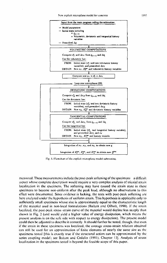
SW txpkit microplanc: model for concrrtr

Input fmm the main pmgram cdling the submutise:

- Model paramcten - Initial state including

l qw1, . Volumetric. deviatoric and tangential history

variables

- Prescribed A<

b VOLUMETRIC COMPUTATIONS

Compute cOy and AE~ from q;_,) and AC

Use the volumetric Iwv:

FROM: Initial state (E: and two volumetric history variables). and prescribed Arv

OBTAIN: New OY. Cvm and volumetric hktory variables

Compute new EY = C: + AEV 1

Ip, Loop over microplanes (28)

I

DEVIATORIC COMPUTATIONS

Compute E: and A~I, from Q,_~, and As

Use the deviatoric Ixw:

FROM: Initial state (CL and two deviatoric history vnriables). and prescribed ACD

OBT~\lN: New oD, c;” nnd dcvintoric history vnrinbles

4

TANGENTIAL COMPUTATIONS

FROM: Init ststc (c;, nnd t;mgcntinl hintory vnrkble). and pruzwibrd ACT, nod cy

OBTAIN. New 0~. , f/i? nnd history vntinbk

Integration of ELM. ELM, and I/!? to obtain new Q’-

mcusurcd. These mc;lsurements include the post-peak softening of the specimens-a ditficult

aspect whose complete description would require a very complex analysis of triaxial strain

locnlizution in the spccimcns. The softening may have caused the strain state in these

specimens to bccomc non-uniform after the peak load, although no observations to this

elTect were documcntcd. Since evidence is lucking. the tests with post-peak softening ;lre

here i~n:~lyzed under the hypothesis of uniform strain. This hypothesis is applicable only to

sutiicicntly smilll spccimcns whose size is approximately equal to the characteristic length

of the material uscrl in non-local formulations (Bu%nnt and Wbolt, 1990). If the strain

locitlizcd, the post-peak stress -strain curve of the material would decline less steeply than

shown in Fig. 1 (and would yield a higher value of energy dissipation, which means the

present iin;tlysis is on the safe side with respect to cncrgy dissipation). The prcscnt model

could then be iidjusted to describe it correctly. It should further be noted, though. that even

if the strain in these spccimcns \vils localized. the average stress-strain relation obtained

can still be used for an approsimrltion of finite elements of nearly the same size as the

specimens tested [this is exitctly true if the structural action can be approximated by the

series coupling model : see Bi&lnt and Cedolin (I 99 I). Chapter 131. Analysis of strain

locrilization in the specimens tested is beyond the feasible scope of this paper.

:"Ii.:w e~plicit microplane model for concrete IISS

IDpu~ from ~he main pro&ram callin, ~he .ubrou~ioe:

- Model parame~rs - Ini~iaJ S~Me iociudin,

• ~.-l) • Volumetric. deviawric and tanseotiaJ hiswry

variables

- Prescribed <3.(

• VOLUMETRIC COMPUTATIONS

Compute ,t. and j.'v from «'_I) and 6,

Use the volumetric law:

FROM: Initial sta~ (!t- and two volumetric history variables). and preocribed 6!v

OBTAIN: New O'v. ~ ... and volumetric history variables

t

I Compute new !v = !t- + 6!v I ~

Loop over microplanes (28)

• DEVIATORIC COMPUTATIONS

Compute!o and 6!0 from ~'_I) and 6,

Usc the deviatoric law:

FROM: Initial st"te ('0 and two deviatoric hiswry v,,,iabl,,,,). "nd preocribed 6!0

OIlTAIN: New" o. E'a" ,,0<\ dcvi"toric hi.wry vllriables

t TANGENTIAL COMPUTATIONS

Cnltll'ut~ !T. "n.\ j.!r. from '<'_I) "nd 6,

Use the t"nKrntiai IIlw:

• 'ROM: Initial stllte (!T. and tangential history variable) • allli p","criLed 6!T. "nd !v

OIlTAIN: N"w "·r •. 11;:- and h •• tory v"ri .. bl"

f lntegrlltion of a'v. if/J. and tiT. 10 obtain new ~

Integration of f:~an. Eh.n I AntI II!:" to obtain new Q'-.n

Fi/,;. 5. Fluwchart 01" the e.\plicit micro plane rnodd subroutine.

mt:asun:d. These me'lsurements include the post-peak softening of the specimens-a ditficult aspect whose completc description would require a very complex analysis of triaxial strain localization in the specimens. The softening may have caused the strain statc in these specimens to become non-uniform after the peak load. although no observations to this elfect were documented. Since evidence is lacking. the tests with post-peak softening are here analyzed under the hypothesis of uniform strain, This hypothesis is applicable only to sutliciently small specimens whose size is approximately equal to the characteristic length of the material used in non-local formulations (Bazant and Ozbolt. 1990). I I' the stmin localized. the post-peak stress ·strain curve of the material would decline less Sl\;eply than shown in Fig. 2 (and would yield a higher value of energy dissipation. which means the present analysis is on the safe sidt: with respect to energy dissipation), The present model could then be adjusted to describe it correctly. [t should further be noted. though, that even if the strain in these specimt:ns was localized. the average stress-strain rebtion obtained can still be used for an approximation of finite elements of nearly the same size as the specimens tested [this is exactly true if the structural action can be approximated by the series coupling model: see Bazant and Cedolin (1991), Chapter 13). Analysis of strain localization in the specimens tested is beyond the feLlsible scope of this paper.

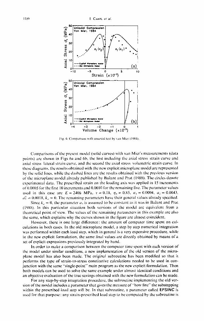
I. CAROL Yl ul.

‘;;; so-

Unloxlal Compr*srIon

: 40. Van Uhr. 1984

.

6- SO’

l . l .

.

;;j 10’ ._ x --c+knluuadwm~od*

< oi ---0d YkmWlW NW*

(0) -10 -5 0 5 10

Strain (x 1tT’)

C’ompurisons of’ lhc prcscnt model (solid curves) ivith van Micr’s mc;Isurcmcnts (dull

points) arc shown in Figs hn and 6h, the tirst including the axial stras strain curve and

axial stress latcr;ll strain curve. and the scco~ltl the asiaI stress volunictric strain curve. In

lhcsc diagxms. lhc rcsul ts ohtaincil with lhc new explicit microplanc model are rcprosontcil

by the solid lines. while the dashctl lines arc the results ohtaincil with the previous version

of the micropl~~nc motlcl already published by IIaiant and I’rat ( I WX). The circles dcnotc

cspcrimcnt;Il data. The prescribed strain on the loadin, 0 axis was applied in I5 incrcnicnts

of0.0005 for lhc first IO incrcmcnts and O.OOlO for the remaining live. The parameter volucs

used in this GISC arc L = 2406 MPa. I’ = 0. IY, qI, = 0.85, (I, = 0.0003. II: = 0.0043.

(1:’ = 0.00 IX. k,, = 0. The remaining paramctcrs have their general values already spcciktl.

Since k,, = 0, the p;lr;lmcter (I, is assu~nctl to bc w11sta11t AS it was in fhlant and Pnlt

(19XS). In this particular situation both versions ot’ the ~noclcl arc ccluivalcnt from ;I

thcorctical point of view. The values of the rcmaininp paranicters in this example are also

the same, which explains why the curves shown in the tigure are al~nost coincident.

Howcvcr. there is one large ditl’crcnce: the amount of computer time spent on cal-

culations in both cases. In the old microplnnc model. ;t step by step numerical integration

was perform4 within each load step, which in general is ;I very expensive procedure, while

in the new explicit formulation. the same linal values are directly obtained by means of ;L

set ofcxplicit expressions previously integrated by hand.

In order to make iI comparison between the computer time spent with each version of

the model under similar conditions. a new implementation of the old version of the micro-

plane model has also been made. The original subroutine has been modified so that it

performs the type of strain-to-stress constitutivc calculi~tions nccdcd to bc used in con-

junction with the same “sir@-point” main program ;ls the new explicit formulation. Then

both models can bc used to solve the same cxamplc under almost identical conditions and

an objective evaluation of the true savings obtained tvith the new formulation can bc made. For any step-by-step integration proccdurc. the subroutine implcmcnting the old ver-

sion of the model includes a parameter that gives the mcasurc of”how tint” the substcpping within the prescribed loiid step will bc. In that subroutine. a paramotcr called EPSlNC is

used for that purpose: any strain-prescribed load step to bc computed by the subroutine is

11~6 I. CAROL 1'1 Ill.

50r-~--~------.-------------~ - Uniaxial Compression ~ Van IooIler, 1984 :::;; 40

o 30

en en IV !; 20 " en " •• ' ~ 10

·x =~...:...'"':"::.:- (0) <: O-l------.----+---~-~~

-10 -S 0 5 10 Strain (x 1 (Tl)

SOr------------.----. - Uniaxial Compression ~ Van IooIler, 1984 :::;; 40 ---0

30 en en IV s.. 20 ....

en

.~ 10 )( = ~..::..:..':"::.:.... (b) <: O---..----.,...---.,...---.J---'~

-4 -3 -2 -1 0 Volume Change (x 1 (Tl)

Fig. h. Comparlsoll with 1Illi;lxlal test hy \all Mi.:r (I'IX-l).

Comparisons of the present model (solid curves) with van Mier's measurements (data points) arc shown in Figs 6a and 60. the first including the axial stress strain curve and axial stress lateral strain curve. and the second the axial stress volumetric strain curve. [n these diagrams. the results ootained with the new explicit mieroplane model an: represented by the solid lines. while the dashed lines arc the results obtained with the previous version of the microplane model already puolished oy Bazant and Prat (19XX). The circles denote experimental data. The prescribed strain on the loading axis was applied in 15 increments of 0.0005 for the first 10 increments and 0.00 I 0 for the remaining five. The p.lrameter values used in this case arc E = 2406 MPa. r == 0.18. '/11 = O.X5. (/1 = 0.0004. (/2 = 0.0043. a'i == 0.00 I X. k" = O. The remaining parameters have their general values already specified.

Since k" = O. the parameter (/ I is assumed to be constant as it was in Iiazant and Prat (19XX). [n this particular situation both versions of the model arc equivalent from a theoretical point of view. The values of the remaining parameters in this example arc also the same. which explains why the curves shown in the figure are almost coincident.

However. there is one large ditTerence: the amount of computer time spent on cal­culations in both cases. [n the old microplane model. a step by step numerical integration was performed within each load step. which in general is a very expensive procedure, while in the new explicit formulation. the same final values are directly obtained by means of a set of explicit expressions previously integrated by hand.

[n order to make a comparison between the computer time spent with each version of the model under similar conditions. a new implementation of the old version of the micro­plane model has also been made. The original subroutine has been modified so that it performs the type of strain-to-stress constitutive calculations needed to be used in con­junction with the same "single-point" main program as the new explicit formulation. Then both models can be used to solve the same example under almost identical conditions and an oojective evaluation of the true savings obtained with the new formulation can be made.

For any step-by-step integration procedure. the subroutine implementing the old ver­sion of the model includes a parameter that gives the measure of"how tine" the substcpping within the prescribed load step will be. In that subroutine, a parameter called EPSINC is usco for that purpose: any strain-prescribed load step to be computed by the subroutine is

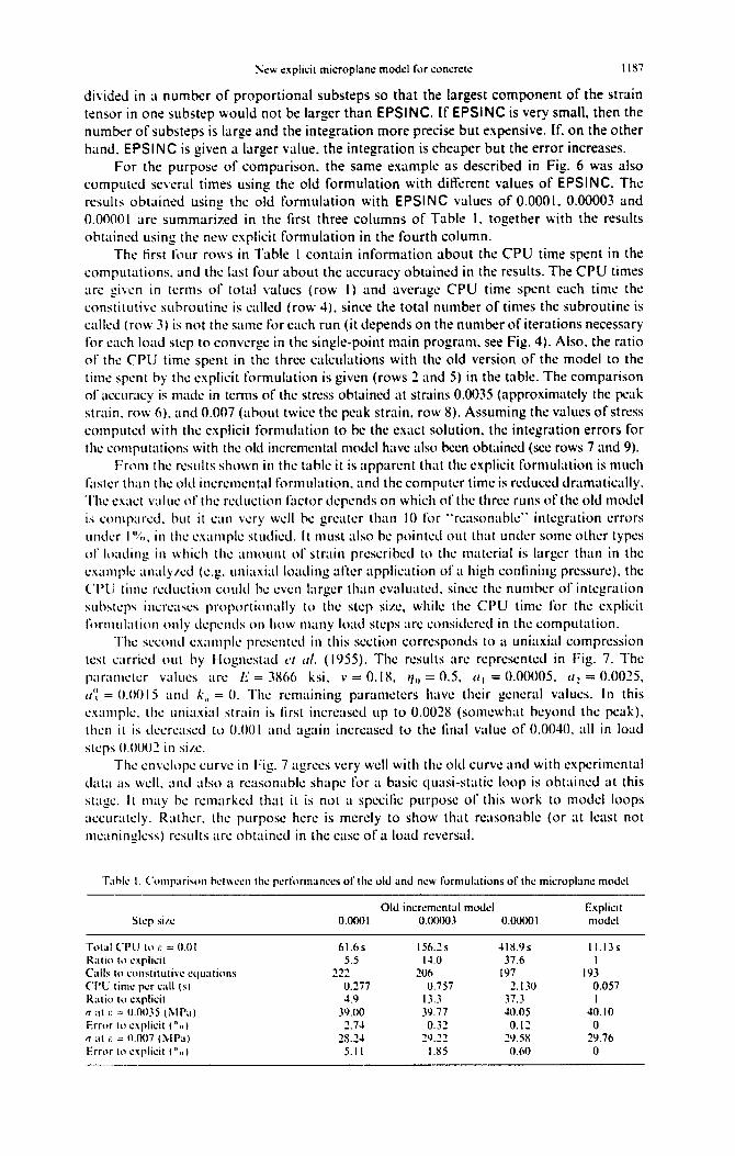
Sew exphcit microplane model for concrek llY7

divided in ;L number of proportional substeps so that the largest component of the strain

tensor in one substep would not be larger than EPSINC. If EPSINC is very small, then the

number of substeps is large and the integration more precise but expensive. If. on the other

hand. EPSINC is given a larger value. the integration is cheaper but the error increases. For the purpose of comparison. the same example as described in Fig. 6 was also

computed several times using the old formulation with different values of EPSINC. The

results obtained using the old formulation with EPSINC values of 0.0001, 0.00003 and

0.00001 are summarized in the first three columns of Table I. together with the results

obtained using the new explicit formulation in the fourth column.

The tirst four rows in Table I contain information about the CPU time spent in the

computations. and the lust four about the accuracy obtained in the results. The CPU times

are pi\-en in terms of total values (row I) and average CPU time spent each time the

constitutive subroutine is called (row 4). since the total number of times the subroutine is

called (row 3) is not the same for each run (it depends on the number ofiterations necessary

for each load step to converge in the single-point main program. see Fig. 4). Also. the ratio

of the CPU time spent in the three calculations with the old version of the model to the

time spent by the explicit formulation is given (rows 2 and 5) in the table. The comparison

of accuracy is made in terms of the stress obtained at strains 0.0035 (approximately the peak

strain. row 6). and 0.007 (about twice the peak strain. row 8). Assuming the values of stress

computed with the explicit formulation to bc the exact solution. the integration errors for

the computations with the old incremental model have also been obtained (see rows 7 and 9).

From the results SIIO~II in the table it is apparent that the explicit formulation is much

faster than the old incrcmcntal formulation. and the computer time is rcduccd dramatically.

The csac~ value of the reduction factor dcpcnds on which of the three runs of the old model

is conip;ircci. hut it can very well hc grcator lhan IO for “rcnsonablc” integration errors

under I ‘X, in lhc cu~iiplc stutlicd. It must also hc pointed out that under some other types

of lo:lding in ivhich the amount of strain prcscribcd to fhc material is larger than in the

cxamplc an;lly/cd (c.g. uni:txial loading after application of a high conlining prcssurc). the

(‘l’li time reduction couhl bc cvcn Iargcr than cvaluatcd. since fhc number of inkgration

suhhtcps incrcascs proportionally lo the stsp size. while the CPU time for the explicit

formulation only tlcpcittls on how ni;iny hid steps arc’ consitlcrccl in the computation.

The second cxaniple prcscntcd in this section corrssponds to ;I uniaxial compression

test carriccl out by llogncs~~l 1’1 111. (1955). The results arc rcprescntcd in Fig. 7. The

paranictcr valiics arc I:’ = MO ksi, v = 0. IX. II,, = 0.5, 0, = 0.00005. ~1: = 0.0025,

11’: = 0.00 I5 ~ntl k,, = 0. The remaining paramctcrs have their gcncral values. In this

cxamplc, the uniaxi:ll strain is tirst incrcascd up to 0.0028 (sonicwhat beyond the peak),

then it is tlccrc;lscd to 0.00 I and again increased to the final value of 0.0040. all in load

stcph 0.0002 in si/.c.

The cnvclopc curve in Fig. 7 agrees very wsll with the old curve and with rxpcrimental

dat;t as well. and also II reasonable shape for a basic quasi-static loop is obtained at rhis

stage. It may bc rcmurkcd that it is not a spccilic purpose of this work to model loops

;lccurately. Rather. lhc purpose hcrc is mcrcly to show that rcasonablc (or at lcast not

mcaninglcss) results arc obtuincd in the cast of a load reversal.

Tahlc I, C’omp;lrk~m hc~~scn IIW pcrliwm;mccs of the old and new formulations of the micropl;mc model

Skp si/c Old incrcmcrkd model Explicit

O.OOOI o.OOOo3 0.0000 I model

61.6s 156.2 5 4lKYs 11.13s 5.5 14.0 37.6 I

1,‘) ___ 206 I97 193 0.277 0.757 2. I30 0.057 4.9 13.3 37.3 I

3Y.00 3Y.77 JI).OS 4O.lO 2.74 0.32 0.12 0

X3.24 29.22 “Y.58 29.76 5.1 I I.85 0.60 0

~.:w .::tpli~it mi~roplane modd for .:on.:ret.: 1187

dividl!d in a number of proportional substeps so that the largest component of the strain tensor in onl! substep would not be larger than EPSINC. If EPSINC is very small. then the number of substeps is large and the integration more precise but expensive. If. on the other hand. EPSINC is given a larger value. the integration is cheaper but the error increases.

For the purpose of comparison. the same example as described in Fig. 6 was also computed several times using the old formulation with different values of EPSINC. The results obtained using the old formulation with EPSINC values of 0.0001. 0.00003 and 0.0000 I are summarized in the first three columns of Table I. together with the results obtained using the new explicit formulation in the fourth column.

The first four rows in Table I contain information about the CPU time spent in the computations. and the last four about the accuracy obtained in the results. The CPU times are given in terms of total values (row I) and average CPU time spent each time the constitutive subroutine is ca1\ed (row 4). since the total number of times the subroutine is ca1\ed (row 3) is not the same for each run (it depends on the number of iterations necessary for each load step to converge in the single-point main program. see Fig. 4). Also. the ratio of the CPU time spent in the three calculations with the old version of the model to the time spent by the explicit formulation is given (rows 2 and 5) in the table. The comparison of accuracy is made in tenns of the stress obtained at strains 0.0035 (approximately the peak strain. row 6). and 0.007 (about twice the peak strain. row 8). Assuming the values of stress computed with the explicit formulation to be the exact solution. the integration errors for the computations with the old incremental model have also been obtained (see rows 7 and 9).

From the n:sults shown in the table it is apparent that the explicit formulation is much faster than the old incremental formulation. and the computer time is reduced dramatica1\y. The exact value of the reduction factor depends on which of the three runs of the old model is compared. out it can very well he greater than 10 for "n.:asonable" integration errors under I '''';'' in the L'.\ample studied. It must also be pointed out that under some other types of loading in whidl the amount or strain pn.:scribcd to the material is larger than in the example analY/ed (e.g. uniaxial loading after application of a high confining pressure), the ('PU time reduction could be even larger than evaluated. since the number of integration suosteps incn:ases proportionally to the step si/e. while the CPU time for the explicit formulation only depends on how many load steps are considered in the computation.

The second example presented in this section corresponds to a uniaxial compression test carried out by Hognestad 1.'1 al. (1955). The results are represented in Fig. 7. The parameter v~"ues arc E = 3X66 ksi. v = O.IX. till = 0.5. al = 0.00005. a~ = 0.0025. a'~ = 0.0015 and k" = O. The remaining parameters have their geneml values. I n this exampk:. the uniaxial strain is first increased up to 0.002X (somewhat beyond the peak). then it is decreased tll 0.00 I and again increased to the final value of 0.0040. all in load steps 0.0002 in si/e.

The envelope curve in Fig. 7 agrees very well with the old curve and with experimental data as well. and also a reasonable shape for a basic quasi-static loop is obtained at this stage. It Illay be remarked that it is not a specific purpose or this work to model loops accurately. Rather. the purpose here is merely to show that reasonable (or at least not meaningless) results arc obtained in the case of a load reversal.

Tahle I. ('omp;lrison hel\\een Ihe perform;ln.:es of the old and n.:w formulalions of Ihe mieroplane mod.:!

Old in.:rement;al mod.:! Expli.:it SICp si/c O.{)(101 0.110003 0.00(101 modcl

Tolal ('I'll 10 I: = (Ull 61.65 156.2s ·W!.9s t 1.13 5 Ralio to c.\plieil 5.5 1-1.0 37.6 t Calls 10 consliluli,.: c<lualions ", 206 197 193 CPU lime per .:all (s) 0.277 0.757 2.130 0.057 Ratio 10 e\plicil -1.9 13.3 37.3 t f7 al r. = 0.0035 (1\.II'a) 39.00 39.77 -10.05 40.10 Error 10 e\plicit (",,) 2.7-1 0.32 0.12 0 f7 al r. = n.007 (Ml'a) 2S.2-1 29.22 29.5M 29.76 Error In nplicil ("" I 5.11 1.85 0.60 0

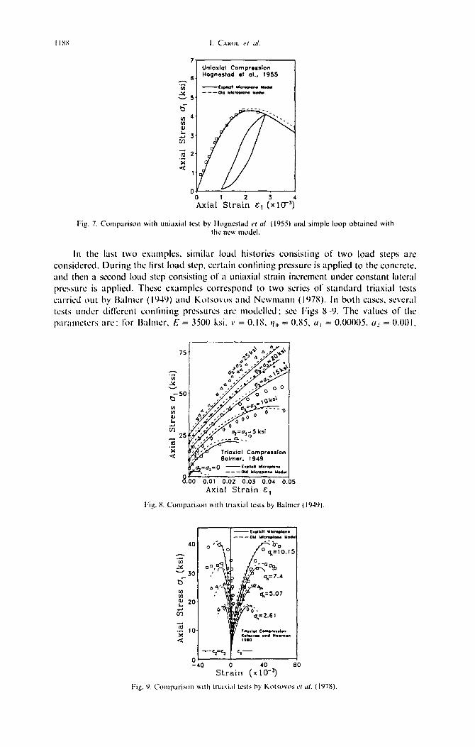
Uniaxial Compr*ssion

ZT 6.

Hognastad et al.. 1955

.z -Fquefl YkawN w ---ad UlsmDiona ygd.

w 5.

-I 0

Axial ‘Slraii El ix IF’;

Fig. 7. Compllrison with unianinl test by Hognrst;td 41 01. (1955) ud simple loop obtGned with the new model.

In the lust two examples, similar load historics consisting of two load steps arc

considrred. During the lirst lo;d step, certain confining pressure is applied to the concrete.

and then a second load step consisting of :I uninxial strain incrcmcnt under constant lateral

pressure is applictl. Thcsc cxan~plcs corrcspontl to two scrics of standard trinxial tests

carrid out by Mtncr (IWO) itntl Kotsovos and Ncwnxlnn (107X). III both CWCS. scvcral

tats untlcr tli!Ycrcnt conlining prossurcs arc ~~~dcllccl; see Figs 8 -9. The villucs OF the

paranictcrs ilK : for Mnicr, E = 3500 ksi. \’ = 0. IS. I/,, = 0.x5. N, = 0.00005. (1: = 0.001.

Balmor. 1949

0 0.01 0.02 0.03 0.04 0.05

Axial Strain El

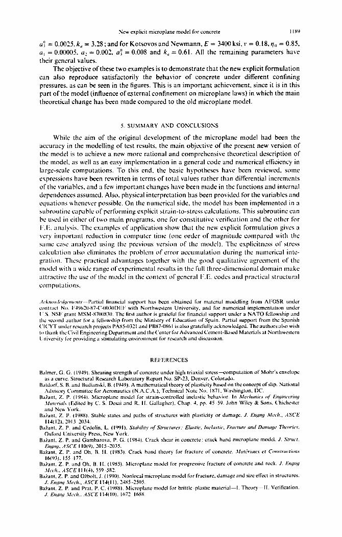
New explicit microplate model for concrete 11x9

u:) = 0.0025. k, = 3.28 ; and for Kotsovos and Newmann. E = WOO ksi. v = 0.18, ‘lo = 0.85.

a, = 0.00005. (I: = 0.001. a: = 0.008 and k, = 0.61. All the remaining parameters have

their general values.

The objective of these two examples is to demonstrate that the new explicit formulation

can also reproduce satisfactorily the behavior of concrete under different confining

pressures. as can be seen in the figures. This is an important achievement. since it is in this

part of the model (influence of -ternal confinement on microplane laws) in which the main

theoretical change has been made compared to the old microplane model.

5. SIJMXIARY ASD CONCLUSIOSS

While the aim of the original development of the microplane model had been the

accuracy in the modellinp of test results. the main objective of the present new version of

the model is to achieve a new more rational and comprehensive theoretical description of

the model. as well as an easy implementation in a general code and numerical efficiency in

larpc-scale computations. To this end. the basic hypotheses have been rcvicwed. some

txprcssions have been rewritten in terms of total values rather than differential increments

of the variables. and a few important changes have been made in the functions and internal

dependcnccs assumed. Also. physical interpretation has been provided for the variables and

equations uhcnever possible. On the numerical side. the model has been implcmcnttxi in a

subroutine capable of performing explicit strain-to-stress calculations. This subroutine can

he used in cithcr of ttvo main programs. one for constitutivc verification and the other for

I-.E. analysis. The cx;~mplcs of application show that the new esplicit formulation gives a

very important reduction in computer Lime (one order of magnitude compared with the

WIIIC cast an:llyxtf using the previous version of the motlcl). The cxplicitncss of stress

calculation also climinarcs the prohlcm of crrur iiccuniulu~ion during the numerical intc-

gration. Thcsc practical advantages togcthcr with the good qualitative agrocmcnt of the

~notlcl with ;I wide range ol’sxpcrinlcntal rcsdb in the fu11 three-tlimcnsion;ll domain make

altractivc rhc use of the niodcl in the contc.ut of’gxcral I:.li. codes and practical structural

compuI;iCons.

,,I~.~,I~J~~~/~~~/~/~~~~I~~~I/.~ --- Parlid lin;mcial support has been obtaincd for matcri;rl modclling from AlX)SR urdcr contract No. I~-1~~61O-X7-C’-lHJ.10L)I:I: with Northwestern University. and for numerical implsmcnt;ition under II.5 NSF grant MSM-X7lHWO. The lirst author is gratsful br financial support under a NATO fellowship and the second iluthor for ;I fellowship from IIIC Ministry of Education ol’ Spain. Partial support from the Spanish C‘IC’Y’I‘ under rsscarch projects PA850321 ;III~ IW7-OXhl is dso gratdully acknowldgcd. The authors ;IISO wish 111 thank thr Civil Engjncering Dcpartmsnt and thcC’cntcr lilr hclv;~ncsd C’cmcnt-Bard Matcrialsat Nodiwsstcrn I!nivsrsiIy for proding ;I stimul;iting unvironmcnt Ibr rcsrarch and discussion.

REI:ERENCES

Balmer. G. C;. (1949). Shearing strength of concrctc under high triaxial srrcss-computation ot’ Mohr’s cnvdopc 1s a curve. Structural Rcscarch Laboratory Report No. SP-23, Denver. Colorado.

H.~tdd. S. H. and Ihdianski. H. ( IYJY). A mathematical theory of plasticity basal on the concept ol’slip. National Advisory Committee for Aeronautics (N.A.C.A.). Technical Note No. 1X71. \C’;lshinglon. DC.

IGant. Z. I’. (IYXJ). Microplanc modsl for strain-controllcd incl;~stic hchat ior. In ZIdrtrnic.~ I)/’ E!@~rirr!/ .I/trtcritr/.~ (Edited by C. S. Dcsai and R. I I. C;all;lghcr). Chap. 4. pp. 35 59. John Wiley & Sons. C’hichcstcr :md New 1’ork.

IG;int. Z. I’. ( IYX~J. Stable st;Ltss and paths of struclurcs with plasticity or damage. J. f$qrfq ,\/rclr.. .d.SC’I:’

I I4 I?). XI 3 203-l.

lhiant. Z. I’. and Ciambarova, P. Ci. (1YX-l). Crxk shear in concrctc: crack band microplans modd. J. .S/rrcc,f. E~lqq. .dSC’E I IO(Y). 2015-3~15.

IWant. Z. P. and Oh. B. I I. (IY85). hlicroplanc model for progrcssivc frxcturc of concrctc and rock. 1. f3,rq~ .t/dl.. :ISC-E I I II-I). 559 -542.

U;G;int. Z. P. and Otbolt. J. (IYYO). Nonlocal microplanc model for fracture. damagr and six cfrccl in structures. J. E,/l/r?cl .\I,‘~lI.. rlSCE I I~( I I). ZJ85-.‘ZO5.

B:riunt. Z. P. and Prat. P. C. (IYRS). Xlicroplanc model for brittle-plastic material-I. Theory-II. Verification. J. Eqqr/!/ .I/dr.. .4SCE I I4 IO). I67;?-lh,YX.

Ncw explicit microplanc moJd for concrete llX9

at~ = 0.OO~5. k. = 3.28; and for Kotsovos and Newmann. E = 3400 ksi. v = 0.18. '10 = 0.85. a I = 0.00005. a~ = O.OO~. a~ = 0.008 and ku = 0.6\. All the remaining parameters have their general values.

The objective of these two examples is to demonstrate that the new explicit fonnulation can also reproduce satisfactorily the behavior of concrete under different confining pressures. as can be seen in the figures. This is an important achievement, since it is in this part of the model (influence of t!"xternal confinement on microplane laws) in which the main theoretical change has been made compared to the old microplane model.

5. SUMMARY Ai'D CONCLUSIO:-';S

While the aim of the original development of the microplane model had been the accuracy in the modelling of test results. the main objective of the present new version of the model is to achieve a new more rational and comprehensive theoretical description of the model. as well as an easy implementation in a general code and numerical efliciency in large-scale computations. To this end. the basic hypotheses have been reviewed. some expressions have been rewritten in terms of total values rather than differential increments of the variables. and a few important changes have been made in the functions and internal dependences assumed. Also. physical interpretation has been provided for the variables and equations whenever possible. On the numerical side. the model has been implemented in a suhroutine capahle of performing explicit strain-to-stress calculations. This subroutine can he uscd in either of two main programs. one for constitutive verification and the other for F.E. analysis. The examples of application show that the new explicit formulation gives a n:ry important reduction in computer time (one order of magnitude compared with the same case anal)'led using the previous version of the model). The explicitness of stress calculation also eliminates the problem of error accumulation during the numerical inte­gration. These practical advantages together with the good qualitative agreement of the model with a wide range of experimental results in the full three-dimensional domain make attractive (he use of the model in the context of general F.E. codes and practical structural com puta (ions .

. ·/ck"oIl1,·d",·11/,·"I.\· ···Partial lin:lIl1:ial support h:IS bt:en obtained for mat.:rial modelling from AI:OSR und.:r .:ontra,t No. F·N620·K7·(,·0030l>EF with Northw.:st.:rn University. and for numerical implementatiun under U.S. NSI: grant MSM·X700XJO. The lirst author is grah:ful for fin:lllcial support under a NATO fellowship and the sewnd author for a lclluwship from the Ministry "I' Education of Spain. Partial support from the Spanish Cl(,YT under rese:lrch projects PA1l5-032I and I'HX7·0Xbl is also gratefully acknowledged. The :\Uthors alsu wish to thank the Civil Enginecring Department and the ('enler for Advarm:d ('.:ment-Based Mat.:rials at Northwestern University for providing a stimulating environm.:nt for research and discussion.

REFERE:-.lCES

Balmer. G. G. (1'.14'.1). Shearing strength of concrete under high triaxial stress-<:omputation of Mohr's envdopc as a curve. Structural Research Laboratory Report No. SI>-23. Denver. Colorado.

Hatdorf. S. B. and Hudianski. B. (194'.1). A math.:maticaltheory of plasticity bascd on the concept of slip. Natiunal Advisory (,ommittee for Aeronautics (N.A.C.A.). T.:chnical Note No. IX7!. Washington. DC.

Ii:liant. Z. P. (I'.IX4). Micrupl:llle model for strain-controlled inelastic behavior. In ;\f.,elum;es of' E"!!;,,t'('T;"!! .\It/It·r;t/ls (Edited by C. S. Desai and R. II. Cialiagh.:r). Ch:lp. 4. pp. 45 59. John Wiley & Sons. (,hich.:ster and N.:w York.

lIai:lnt. Z. 1'. (llJKX). Stable states and paths of structures with plasticity or damage. 1. E".l/".cJ Mel'It .. AS('/:' 11-&( (2). 20 tJ 20J4.

Oai.:lllt. Z. P. and Cedolin. L. (19'.11). Stt/hility "f StrtlCllm:s,' Elasl;e. I"dt/st;c. FmCllm' and Dalllt/5I" TIt,·or;t's. O~lilrd liniversity Press. New York.

Baiant. Z. P. and Gambarova. P. G. (19114). Crack shear in concr.:te: crack band microplane model. 1. StrtlCI. E".t/ll.q. ASCE 110(9). 2015-20J5.

B:Ii.;lIIt. Z. P. :lIId Oh. n. II. (I'.IX). Cr .. ck band thellry for fr:\Ctur.: or coner.:t.:. J/t/It'r;t/IlX .'1 ('""strllcl;on, 16(93).155 177.

Baian!. Z. P. and Oh. B. II. (l9X5). Microplane model ror progressiv.: fracture of concrete and rock. 1. {:."5I"!! .\It'dl .. ASCE 111(4). 559 -5112.

Balant. Z. P. and Oi.bolt. J. (1990). Nonlocal microplane model for fracture. damage and size elTect in structures. 1. E"tlnq .\I .. clt .• .-IS(, E 11-&( II). 24X5 .. 2505.

Bazant. Z. P. and Prato P. C. (l9SXl. Microplanc model for brittle·plastic material-I. Theory-II. Verification. 1. £".<I"!' .Ift·c/r .. AS(,E 11-&( (0). 1672-16SX.

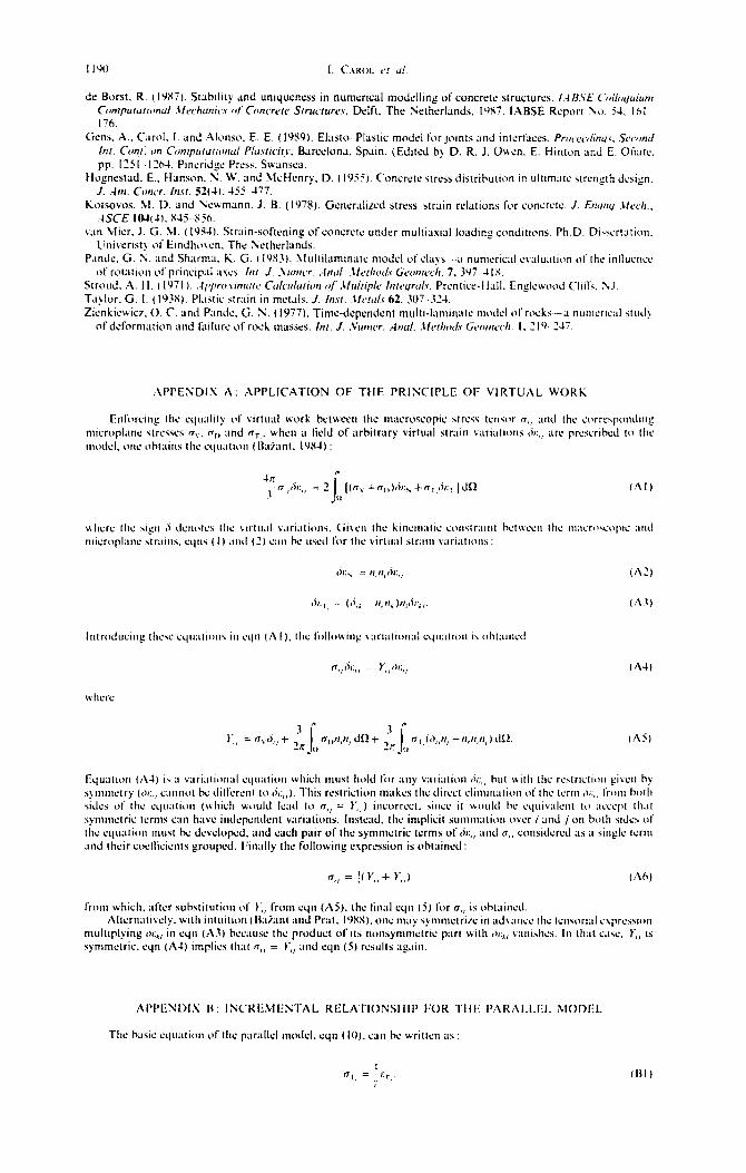
I IYO I. C.\HOL Cl d.

Hupnestad. E.. Hanson. N I%’ and McHicnry. D. lI9i5). Concrctr stress distribution in ultimate strength deign. J. .4m. C0nc.r. Insr. 53-r). 455.-177.

~otsovos. hl. D. and Sewmann. J. B. (1978). Gencrahxd stress-strain relations for concrctc. J. Empty .\lrch.. .4SCE IoJ(-1l. x-I5- S56.

van Slier. J. G. .\I. ( IWU). Strain-softening ofconcretc under multiuutal loudins conditions. Ph.D. Dtwrtxtwn. L;nivrrtst~ of Eindhoben. The Netherlands.

APPCSDIS A: APPLICATION OF THE PRISCIPLE OF VIRTUAL WORK

Enliwctng the cqual~ty of vtrtual work between the macroccopic strew ten%ior m,, and the c’c~rwpondlng micropl;~nc ctrswcs 0,. f-r,, and n,,. when a tield of arbitrary virtual str;lin vartations (jr:,, iire prcscrlhcd to the model. wit obtains thc cqu;1110n (tkktnt. IYXJ) :

Jn

! n,,rir:,, = 2 1’ [(CT, + fl,, )A:, + n , ,&I:, ,I do (.A I J

II

OI:, = ti,,i,ril: I,

(/\7)

r;, = CT,&,, + 3~ i n,,n,n, dS! +

3 In 0 2n

I n,,(ri,,n, -rr,n,n,J 1111. 0

(AS)

Equ;ltion (Al) i\ ;I variarwlal equation which must tu)ld liar any v:lrlation A:,( hut ulth the rc~~rIctIon gikcn hy ,)mmctry (a.., cannot bc dili’crcnt to A,,). This rrstrictiw makes the direct climln;ltion ofthc term oi.,, from both a&s of the quation (uhlch ~(wld lad to n,, = I’,,) incorrccl. sincc it would hc cquiv;IIcnI tu ;~cccpt 111.11

symmrtric terms can have indcpcndcnt wriations. Ins~cad. ths implicil summation wcr i and i on both sides ol the cquatiw mu>~ bc dcwlopcd. and each pair of the symmetric trrms of A:,, and 0,, considsrod as a stnglc tsrni and their cwllisicn~s grouped. f:in;dly the following expression is ohtainrd :

“,, = icy,,+ I;,, (/\hJ

from which, after whstitution of 1.,, from CL~II (A5). the linal cqn (5) liw n,, is oht;linud. r\ltcrn2ti\sly. with inluilioii ( IWan~ :lnd I’ral. IYXX). one’ rn;l) *)rnmctri~ in ad\;tncc the Icn~w~l c\prcAon

multiplying A:,, in cqn (A3) hcc;lusc the product of ils nonsymmctric parI with A:,, v;mi&s. In that C‘;IX. r,, 1s symmetric. qn (A-t) implies that n,, = Y :Ind ccln (5) results aqin. ,,

APPESDIS IS: IS<‘REMENTAL RELATIONSIIII’ FOR TIIT: l’,\R;\I.LI:I. MODEL

The basic qualion of the paraM model. cqn ( IO). can hc rbrittcn ;IS :

11'lt) I. C\I{()L t' [ ul.

dt: Borst. R. (I'lS7). Stability and uniqut:nt:ss in numt:ri.:al moddllng of wneret.: stru\:tun:s. I ~8SE Colloquium Co",{'tIlut/unul .\ft'chanin ,,( Conaete Structures. Delft. The ~etherlands. I\lX7. L\BSE R.:port :\0. 54. I hi 176.

Gens. A .. emll. I. and Alonso. E. E. (19S9). Elasto .. Plasti.: mod.:! for joints and interfaces. Pro('f!(·dinl./s. Second In[. COIl( on ComplI[ullOllal Plas[iciey. Bar.:dona. Spain. (Edited by D. R. 1. Ov.en. E. Hinton and E. Onate. pp. 125112~. Pineridge Press. Sv.ansea.

Hognestad. E .. Hanson. :\' W. and I\h:Henry. D. (1955). Concrete stress distrioution in ultimate strength design. J. Am. COller. In.H. S:!(41. 455·-H7.

Kotsovos. 1\1. D. and :\ev.mann. J. B. (I\l7!)). Generalized stress .. strain rdations for com:retc. J. EIII./I1I./ .\fech .. ASCE 10-'(41. S45 .. ~56.

van Micr. J. G. \1. (1\l~4). Strain-softening of .:oncrete under multiaxialloading \:onditions. Ph.D. Di,scrtation. Univeristy of Eindhoven. Tht: :'-Ietherlands.

Pand.:. G. :\. and Sharma. K. G. (19S3). Multilaminate modd of .:Iays-"'I numerical evaluatilln of the inlluem:e of rotatil1n llf prin,ipal 'I.,es. 111[.1. :Vufllcr. Anal .. \fc[hod,· Geofllccil. 7. 3'l7 -' I X.

Stfllud. A. H. (1\l71) . . ~rrru\,/flla[C CalCIIla[ioll ot' JIIII[irle Illlcqral,. Pn:ntice-Hall. Engkw(lOU Cllt]'s. :\J. T.lylor. G. I. (1\l3SI. PI,lstic strain in metals. J. 111.1'1 .• \tc[a!., 62.307 324. Zienkicwicz. O. C. and Pande. G. N. (1977), Time-dependent multi-laminate model (If fllcks-a nurneri,al study

of deformatilln and f,lilure of fll.:k masses. Int. J. ,vlllller. Af/al. Jfe[ho,l>' Geolllcch. I. 219· 247.

APPENDIX t\: APPLICATION OF THE PRINCIPLE OF VIRTUAL WORK

Enforcing till" equality (If virtual work octween the malTosc(lpic stre" h:nS(lr fT" and the corresponding mi.:roplane stn:"l'S fT\,. fT" and "r.' when a tield of aroitrary virtual str<lin variations ,i.:" arc presnioed ttl the l\1odel. OIiC llotains the clJuatlon (Baiant. Illi(4):

(i\ I )

where thc si..:n ,i denolcs thc virtual variations. (iivl'n thc kincmatic ,onstraint hctwwn the 1I1;lI:ro'l·opi.: and microplane ;trains. elJns (II and (~) can he used ror the virtual stralll variatlllfls:

IntrodllL:ing these equations in eqll (i\ I). thc foll,lwillg variational .:qnation is ohtalll.:d

where

Equation (A41 is a variational cquation whidl must hold lilT any variation Ii.:" hut with th.: rcstnL:tion givcn hy symmctry (I)':., cannot tx: dilJ'crent tll ,i.:,,). This rcstridion makes the direct diminalion of the term Ill:" rwm hOlh sidcs or thc equation (whi.:h would lead to 11" = Y,,) in.:orrccl. since it would he elluivalent to a,'L:ept thaI symmetric terms can havc independent v;lriations. Instead. the implicit summation ovcr i and i on both sides of the equation must oe uevdoped. and c;lch pair of the symmctric terms of ,il:" and 11" considered as a single I<:rm and their coelli.:ients grouped. Finally the following e:\pn:ssion is ohtaincd :

11" = l(Y,,+ Y,,) (Ah)

from which. aftcr suhstitution of Y" from eqn (A5). the linal eqn (5) for 11" is ohtaincd. Alt.:rnativdy. with intuilion (lIa,;ant and I'rat. 19K5). one l\1ay s}l\1l\1elri/e in adv;lIll'e thc tensllri;d "prcssion

Illultiplying ,i/:" in e'ln (A3) hecause the produd of its n"nsymmetric part with Ii.:" vanishes. In that C'ISC. Y" is symmctric. eqn (A4) implies that fT" = Y" and eqn (5) rcsults again.

APPE~()IX B: I~(,REMENTAL RELATIONSIIIP FOR TilE P,\RALl.EI. MODEL

Th.: oasic equation elf thc par.dld model. eqn (H)). can oc writtcn as:

r rTr. = .,r.T ., ,

(III)

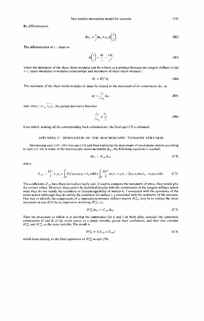
SW explicit mkropl;lnr model for concrete

By dilferentiutron.

I I91

(82)

The difkrentiution of r ;’ lrdds to

d tB3)

where the increment of the shear stress modulus can tx urittcn as ;L product between the tangent stitTness in the r-y space (modulus to modulus relationship) and incrcmrnt of shear strain modulus:

dr = E’“” d-.. r , (B-L)

The increment of the shear strain modulus d;, must be related to the increment of its components dcr, as

_- and. since ;’ = , cr cr , ,. the partial dcrivativc kames

(BS)

(Rh)

from which. making all the corrcspcmding h;l~)i-sclhstitutions. the Cnal cqn ( 17) is ohtaincd

/\PI’I;Sf~IS (‘: DERIVATION 01: TIIE M/\C‘KOS(‘OI’I(‘ TANCiENT STII’I‘NISS

l’hc cocllicicnts Z,,,, have hccn &rived c0rrcctly and, if used (0 compute lhr incrcmcnt of stress, they would pivc thr correct v;iIucs. I It)ucvcr. they c;mnol hs idcntilicd directly will1 lhc ctmlponcnts of the tangent still’ncss tensor sincc thsy do n~)t satibfy the condition of intcrcti;lllgc;lhility of indicts k, / x~socia~cd with the symmetry of thr strain tcnror (although they &r satisfy the condition liu indiccs i, j associakd wiUl the symmstry of the strcsscs). One way lo identify the comp~~ncnts of a syllllllctry-ct)nsiklccilt stili‘ncss mxtri.x f)$,. may hc (~1 rcplxc lhc ‘itruss

Incrcmcnt in cc111 (Cl) hy its cxprcsxitrn involving f>$‘,, ix

I)‘.“’ dl. = % ,111 “I dr ,111 “I (C3)

‘fl~cn the procsdurc IO follow is to d~Aop the summ:ltion for k and I on both sides. consider thr symmetric components kl and lk of the z,train tensor as ;l single variahlc. group their cucllicicnts. ~riicl 1lic11 ;ilso amsider

n:;;, and D,;,, "'I ~1s lhs same vari;ihlc. m result is

,)‘“” = l,l, ifir,,,, +%,,,I (C’J)

which Icads dirLvtly to thr linal cxprsssion of /):T;‘, in sqn (IV)

:-';.:W expli..:it mi..:roplan.: modd for ..:oncret.: 119 I

By ditf.:rentiation.

The differentiation of,: :' leads to

(B3)

where the incn:ment of the shear stress modulus can be written as a product betwe.:n the tangent stiffness in the t-;' space (modulus to mlldulus relationship) and increm.:nt of shear strain modulus:

dr = E'r'" d;',

The increment of the sh.:ar strain modulus d;' must be rdated to the increment of its compo",:nts d,: r, as

(B5)

and. since ;' = ,,'I:r/ r,. the partial derivative henllnes

(Rfi)

fwm whidl, making all the corn:sp(lflding hack·suhstitutions. the linal eqn (17) is ohtained,

APPI,NDL\ C: OERIVATION OF TilE MACROSCOPIC TANGENT STIITNESS

Inlwdudng eqlls (14) (Ill) into eqn (1.1) and then repladng the in..:relllents of Illicwplane straills according 10 eqns (I) (4) in terllls of the llla.:nlS,:('pi.: strain i",;relllent It.:H• the following equalion is readIed:

(CI)

where

The .:oellkients Z"H have heen derived correctly ami. if used to eOlllpule Ihe increment of stress. they would give the correct values, Ilowever. they cannot he identilied directly with the components of the tangent still'ness tensor sin.:e they do not satisfy the condition of interchangeability of indices k. I asso..:iated with the symllletry of the strain h:nsor (although they do satisfy the condition I".r indices i. i associated with the symmetry of the stresses), One way to identify the cOlllponents of a symmetry-consistent slill'ness l1lalri.\ 0:;:'" may be to n:place the slress incrcment in eqn (el) hy its cxpression invol~ing f):;'~,. i,e,

(e3)

Then the procedure to follow is to devdop the summation for k and Ion both silks. consider the symmetric components kl and Ik of the strain tensor as ;1 singk variable. group their cuellieients. and then also consider 0:;:'/ and D:;:: as the same variahlc, The result is

which le;lds dir~'Ctly to the Iin;1I expression of 0:;:', in eqn (19).