New Evidence on the Finite Sample Properties of

Propensity Score Reweighting and Matching Estimators∗

Matias BussoIDB, IZA

John DiNardoMichigan, NBER

Justin McCraryBerkeley, NBER

June 9, 2011

Abstract

The existing literature comparing the finite sample properties of reweighting and matching estimators ofaverage treatment effects concludes that reweighting performs far worse than even the simplest matchingestimator. We argue that this conclusion is unjustified. Neither approach dominates the other uniformlyacross data generating processes. Examining data generating processes mimicking standard microeco-nomic data sets, we conclude that reweighting is more effective than matching estimators when overlap isgood, but that nearest neighbor matching, possibly with bias-correction, is more effective when overlapis sufficiently poor.

JEL Classification: C14, C21, C52.

Keywords: Treatment effects, propensity score, matching, reweighting.

∗For comments that improved the paper, we thank Alberto Abadie, Matias Cattaneo, Keisuke Hirano, Guido Imbens,Pat Kline, and seminar participants at Berkeley, Wisconsin, and the Atlantic Causal Inference Conference, but in particularBryan Graham, Jack Porter, and Jeff Smith. We would also like to thank Markus Frolich for providing us copies of the codeused to generate the results in Frolich (2004).

I. Introduction

A common goal of empirical work is to assess the impact of a non-randomized program on a subpopulation

of interest. Estimates of program impacts are often based on matching on covariates or the propensity

score or reweighting. Empirical literatures, particularly in economics, but also in medicine, political sci-

ence, sociology and other disciplines, feature an extraordinary number of program impact estimates based

on these estimators. Propensity score matching is particularly popular and is described by Smith and Todd

(2005) as “the estimator du jour in the evaluation literature.”

In a recent article in the Review of Economics and Statistics, Frolich (2004) uses simulation to examine

the finite sample properties of various propensity score matching estimators and compares them to those of

a particular reweighting estimator. To the best of our knowledge, this is the only paper in the literature to

explicitly compare the finite sample performance of propensity score matching and reweighting. The topic is

an important one, both because large sample theory is currently only available for some matching estimators

and because there can be meaningful discrepancies between large and small sample performance.1 Summa-

rizing his findings regarding the mean squared error of the various estimators studied, Frolich (2004, p. 86)

states that the “the weighting estimator turned out to be the worst of all [estimators considered]... it is far

worse than pair matching in all of the designs”. This conclusion is at odds with some of the conclusions from

the large sample literature. For example, Hirano et al. (2003) show that reweighting can be asymptotically

efficient in a particular sense. This juxtaposition of conclusions motivated us to re-examine the evidence.

We build on the previous literature by presenting evidence on the finite sample performance of a broad set

of matching and reweighting estimators over a broad set of data generating processes (DGPs). We consider

nearest neighbor matching on covariates and on the propensity score with and without bias-correction, local

linear matching on the propensity score, and three types of reweighting estimators. Regarding DGPs, we

consider those based on hypothetical data studied in the previous literature, as well as more empirical DGPs

based on the Current Population Survey (CPS) and the National Supported Work (NSW) Demonstration.

We conclude that reweighting is a much more effective approach to estimating average treatment effects

than is suggested by the analysis in Frolich (2004). In particular, we conclude that in finite samples an ap-

propriate reweighting estimator nearly always outperforms pair matching. Reweighting typically has bias

on par with that of pair matching, yet much smaller variance. Moreover, in DGPs where overlap is good,

reweighting not only outperforms pair matching, but is competitive with the most sophisticated matching

estimators discussed in the literature. This is an important finding because reweighting is simple to imple-

1Large sample properties of these estimators are studied in Heckman, Ichimura and Todd (1998), Hirano, Imbens andRidder (2003), Lunceford and Davidian (2004), and Abadie and Imbens (2006), among others.

1

ment, and standard errors are readily obtained using two-step method of moments calculations. In contrast,

sophisticated matching estimators involve more complicated programming, and standard errors are only

available for some of the matching estimators used in the literature (Abadie and Imbens 2006, 2008, 2010).

On the other hand, in DGPs where overlap is poor, reweighting tends not to perform as well as some of

the more effective matching estimators. One of the most effective of these is bias-corrected matching with

a fixed number of neighbors, which fortuitously is one of the matching estimators for which standard errors

are available. Because the relative performance of estimators hinges so powerfully on features of the DGP,

we suggest that researchers estimate average treatment effects using a variety of approaches; researchers

may further want to conduct a small-scale simulation study focused on the empirical context at hand.

The remainder of the paper is organized as follows. Section II defines notation and estimators. In Section

III, we replicate and extend the findings of Frolich (2004). We focus on two key issues. First, we consider

matching and reweighting on the estimated propensity score, rather than the true propensity score, and we

further examine the performance of several estimators not considered in that article, including normalized

reweighting and bias-corrected matching. Second, we show that a seemingly minor change to the DGPs

used in Frolich (2004)—namely increasing the variance of the outcome equation residual—dramatically

affects the relative performance of these estimators. In Sections IV and V, we consider estimator perfor-

mance in the context of two DGPs that are more empirically grounded. The first of these pertains to

estimation of the black-white wage gap in the CPS. The second pertains to estimation of the effect of job

training in the NSW observational data. In Section VI, we discuss the results of a series of DGPs where

we manipulate the overlap in the NSW and CPS designs. Section VII concludes.

II. Background

The starting point for much of the traditional program evaluation literature (e.g., Maddala 1983, Sec-

tion 9.2, Heckman and Robb 1985, Maddala 1986) is the model

Yi(t) = µt(Xi) + εti (1)

T ∗i = µT (Xi)− Ui (2)

where t ∈ {0, 1} indexes treatment assignments, Yi(t) is the outcome under treatment assignment t, Xi is

a covariate vector, and Ui and (ε1i , ε0i ) are mean zero and independent of Xi.

2 The data observed by the

researcher are (Yi, Ti, Xi)n

i=1, where Yi = TiYi(1) + (1− Ti)Yi(0) and Ti = 1(T ∗i > 0).

The key sufficient conditions for identification of average treatment effects are conditional independence

2Note that we are not subscripting µT (·) by n. That is, we adopt an infinite-population perspective under which overlapis neither getting better nor getting worse as the sample size grows.

2

and overlap, although√n-consistency may require a strengthening of the overlap assumption to strict

overlap (Khan and Tamer 2007). Conditional independence here means that Ui is independent of (ε1i , ε0i )

conditional on Xi. Strict overlap means that for some c > 0, we have c < p(x) < 1 − c for almost every

x in the support of Xi, where p(x) = P (Ti = 1|Xi = x) is the propensity score. Overlap allows c = 0. See

Imbens (2004) and Khan and Tamer (2007) for discussion.

There are many possible parameters of interest associated with the model in equations (1) and (2). The

literature focuses primarily, although not exclusively, on two parameters: the effect of treatment on the

treated (TOT), defined as E[Yi(1)− Yi(0)|Ti = 1] ≡ θ, and the average treatment effect (ATE), defined as

E[Yi(1)− Yi(0)]. Following Smith and Todd (2005) and others, we focus on TOT.

Aside from bias-corrected matching, the matching estimators we examine can be written as

θ =

∑i Ti{Yi − Yi(0)

}∑i Ti

(3)

where the sums are over all of the data, Yi(0) =∑

j (1− Tj)W (i, j)Yj/∑

j (1− Tj)W (i, j) is the out-of-

sample forecast for treated unit i based only on control units j, and the function W (i, j) gives the distance

between observations i and j in terms of either covariates or propensity scores. Table 1 gives the W (i, j)

function for nearest neighbor matching on the propensity score, nearest neighbor matching on covariates,

and local linear matching on the propensity score.3

For propensity score based estimators, we use an estimate of the propensity score, rather than the true

propensity score. The rationale for this choice is that it is unusual to find empirical applications in which

the true propensity score is known. Even when it is known, it is nonetheless typical to estimate it (e.g.,

Kling, Liebman and Katz 2007), since doing so improves efficiency for both matching and reweighting

(Hirano et al. 2003, Wooldridge 2007, Abadie and Imbens 2009). We use a parametric approach where the

propensity score model is fixed across samples and the complexity of the model is modest relative to the

number of observations.

The other matching estimator we study is bias-corrected matching. This approach is motivated by the

finding that nearest neighbor matching is inconsistent when matching more than one continuous variable

(Abadie and Imbens 2006). The idea is to subtract an estimate of the asymptotic bias of nearest neigh-

bor matching from the nearest neighbor matching estimator itself. Abadie and Imbens (2011) propose

estimating the asymptotic bias using linear regression, and we follow that proposal here.4

3For the local linear estimator, we use the Epanechnikov kernel and further apply the finite sample adjustment to thedenominator proposed in Seifert and Gasser (1996, 2000). Frolich (2004) refers to this estimator as “ridge matching”.

4Bias correction for nearest neighbor matching on the propensity score uses linear regression with the estimated propensity

3

Matching estimators require the researcher to choose one or more tuning parameters. Nearest neighbor

matching requires choosing a number of neighbors, and local linear matching requires choosing a band-

width. The choice of number of neighbors is in some sense easier, because k = 1 (pair matching) is a

natural conservative default, whereas there is no natural conservative default for choosing a bandwidth.

We consider the cross-validation procedure seen most commonly in the literature. For nearest neighbor

matching, this procedure chooses a number of neighbors, k, to minimize

Q(k) =∑j

(1− Tj)(Yj − Y−j,k)2 (4)

where Y−j,k =

∑`(1− T`)Wk(`, j)1(` 6= j)Y`∑`(1− T`)Wk(`, j)1(` 6= j)

(5)

is the out-of-sample forecast for control unit j based only on control units ` 6= j, and where we write the

matching function as Wk(i, j) to emphasize the dependence on the number of neighbors. Cross-validated

bandwidth selection is analogous.5 An emerging literature considers cross-validation routines specialized

to this context (e.g., Galdo, Smith and Black 2010), but we leave a full consideration of competing cross-

validation proposals to future research.

In summary, we report results for 11 matching estimators: pair matching on the propensity score and

on covariates; 4th nearest neighbor matching on the propensity score and on covariates, with and without

bias-correction; nearest neighbor matching on the propensity score and on covariates with the number of

neighbors chosen by cross-validation, with and without bias-correction; and local linear matching on the

propensity score with the bandwidth chosen by cross-validation.6

In addition to matching estimators, we study unnormalized reweighting, normalized reweighting, and an

estimator due to Graham, Campos de Xavier Pinto and Egel (2009, 2010), which we term GPE reweighting.

Unnormalized and normalized reweighting estimators are given by

θU =

∑i TiYi∑i Ti

−∑

j(1− Tj)WjYj∑j Tj

(6)

θN =

∑i TiYi∑i Ti

−∑

j(1− Tj)WjYj∑j(1− Tj)Wj

(7)

respectively, where Wj = pj/

(1 − pj) and pj = Λ(Z ′j π) is the estimated propensity score for unit j based

on a logit model, where Λ(t) = 1/(1 + exp(−t)) and Zi is a vector of functions of Xi including a constant

score as a regressor, and bias correction for nearest neighbor matching on covariates uses linear regression with Xi as a regressor.5For n < 400, we evaluate Q(k) for k ∈ {1, 2, . . . , 20, 21, 25, 29, . . . , 53,∞}. For n ≥ 400 we evaluate Q(k) for

k ∈ {1, 2, 3, 4, 5, 6, 8, 10, . . . , 20, 40, 60, . . . , 100,∞}. We evaluate Q(h) for h = 0.01× 1.2g−1 for g ∈ {1, 2, . . . , 28, 29,∞}.6For matching on covariates, we use the Euclidean metric.

4

term. We choose a small number of functions of Xi, consistent with the parametric perspective we adopt.

GPE reweighting is given by equation (7), but pj is not based on a logit model. To explain the

approach, note that if the true propensity score is of the form Λ(Z ′iπ0) for some parameter π0, then

0 = E[(Ti − Λ(Z ′iπ0))g(Zi)] for any function g(·), suggesting by the analogy principle a class of moment-

based estimators for the propensity score indexed by g(·). The logit model uses g(Zi) = Zi. GPE reweight-

ing with logit functional form uses g(Zi) = Zi/(1 − Λ(Z ′iπ0)). This leads to exact finite-sample balance,

or∑

i TiZi/∑

i Ti =∑

j(1− Tj)WjZj/∑

j(1− Tj)Wj , and thus regression adjustment for Zi is redundant

in the reweighted sample. This redundancy makes GPE reweighting double-robust in the sense of Robins,

Rotnitzky and Zhao (1994): the estimator is consistent if either the propensity score model is correctly

specified, or if the µt(Xi) functions are linear in Zi.

These three variations of reweighting differ in their prominence in the literature. GPE has only recently

been proposed and so has not been extensively studied or used in empirical work. However double-robust

estimators more broadly have been studied extensively in the recent theoretical statistics literature. The

unnormalized reweighting estimator dates at least to Horvitz and Thompson (1952) and features promi-

nently in the theoretical statistics and econometrics literatures. The normalized reweighting estimator

receives little attention in the theoretical literature, but features prominently in empirical work.7 In our

context, normalized reweighting is of particular interest because the matching estimators listed in Ta-

ble 1 can be interpreted as normalized reweighting estimators.8 Consequently, a meaningful comparison of

matching and reweighting requires that the normalized reweighting estimator be considered.

III. Previous Results

We turn now to a re-examination of the performance of propensity score reweighting and matching esti-

mators in the context of the DGPs utilized by Frolich (2004). Those DGPs can be expressed as

Yi(0) = m(Xi) + εi (8)

T ∗i = α+ βΛ(√

2Xi)− Ui (9)

with Yi(1) = Yi(0) and Ti = 1(T ∗i > 0), where α and β are parameters given in Table 2, and m(·) is one of

a set of functions specified in Table 3.9 The covariate Xi is independent and identically distributed (iid)

7A brief list of prominent references discussing the unnormalized estimator, but not the normalized estimator, includeRosenbaum (1987, Equation (3.1)), Dehejia and Wahba (1997, Proposition 4), Wooldridge (2002, Equation (18.22)), andHirano et al. (2003, pp. 1175-1176). The normalized reweighting estimator is discussed in Lunceford and Davidian (2004),Imbens (2004), and Robins, Sued, Lei-Gomez and Rotnitzky (2007), for example.

8Short proof: Define Vj ≡ n−11

∑i TiW (i, j), where n1 =

∑i Ti. By the definition of W (i, j), we have

∑j(1−Tj)Vj = 1 and

then n−11

∑i TiYi − θ = n−1

1

∑i Ti

∑j(1− Tj)W (i, j)Yj = n−1

1

∑j(1− Tj)Yj

∑i TiW (i, j) =

∑j(1− Tj)VjYj/

∑j(1− Tj)Vj .

9Strictly speaking, Frolich (2004) does not use a model for Yi(1) at all. This omission is motivated by the recognition that

5

standard normal. The residual Ui is iid standard uniform, and εi is iid uniform with a mean of zero and

a variance of 0.01. These residuals are mutually independent and independent of Xi.

There are five combinations of α and β and six functional forms for m(·), for a total of 30 DGPs. The

propensity score for this DGP is given by p(x) = α+ βΛ(√

2x). We approximate this using a logit model

with Zi representing a cubic in Xi; GPE reweighting uses a logit functional form with the same Zi as a

covariate. Figure 1 presents population overlap plots for the five combinations of α and β (“designs”).10

Figure 2 presents the curves used for m(·). These functions exhibit a range of shapes, from approximately

low-order polynomial (e.g., curves 1 and 4) to highly nonlinear (e.g., curves 2 and 6).

Asymptotic approximations suggest that these designs favor matching over reweighting. First, nonlin-

earity of the outcome curves increases the asymptotic variance of reweighting more than that of matching

estimators in the nearest neighbor family.11 Some of the curves in Figure 2 are quite nonlinear. Second,

the logit model that we use for estimation is consistent only for the propensity score for design 1, which

sets α = 0 and β = 1. Designs 2 through 5 do not satisfy any standard latent variable model setup, and

reweighting may not be consistent. Third, while the logit model is well specified for design 1, strict overlap

is violated, thus presenting a challenging setting for reweighting.12 On the other hand, some outcome

curves can be well-approximated by a third degree polynomial, suggesting small bias for GPE reweighting.

Below, we discuss the somewhat surprising result that the variance of εi has a powerful impact on the

relative performance of matching and reweighting estimators. We show this in a simple way, by presenting

results based on the exact DGP used in Frolich (2004), which sets V[εi] = 0.01, and then later conducting

the same analysis with V[εi] = 0.10.

For each of the 30 DGPs outlined, we construct 10,000 samples of size n = 100 taken randomly with

replacement from the population model described in equations (8) and (9).13 Schematically, each sample is

constructed in six steps: draw iid standard normals Xi; draw iid standard uniform errors Ui; construct T ∗i

according to equation (9); assign Ti = 1(T ∗i > 0); draw iid uniform errors εi with mean zero and variance

equal to either 0.01 or 0.10; and finally construct Yi(0) = Yi(1) = Yi according to equation (8).14

the DGP for Yi(1) does not affect the relative performance of estimators for TOT. We prefer to be able to discuss the resultsin terms of traditional notation and models, however, and use the convention that Yi(1) = Yi(0).

10The conditional density of the propensity score given treatment is given in Part IA of the Web Appendix.11See Part IB of the Web Appendix for these results.12Strict overlap is a sufficient condition for

√n-consistency but is not a necessary condition. It may be shown that reweighting

is√n-consistent for these DGPs, and indeed for all those considered in this paper. See Part IC of the Web Appendix.

13Programming of estimators and construction of hypothetical data sets was performed in Stata, version 11.0. See Part IDof the Web Appendix for discussion of some important details regarding pseudo-random number generation.

14To economize on computing time, we fix the draws of the covariate and the outcome error to be the same within eachdesign. Formally, in our overall data set of simulated outcomes, the data are organized as Yicdr = mc(Xidr) + εidr, where ris a replication, d is a design, c is a curve, and i is an observation.

6

Using these samples, we construct simulation estimates of the bias and variance.15 These results are

presented in Tables 4 (bias) and 5 (variance). We turn first to the results on bias. For readability, the

simulation estimates of bias are all scaled by 1000. Columns in Table 4 correspond to estimators and rows

correspond to DGPs. The bottom of the table presents three additional rows with summary statistics for the

preceding 30 rows. The first row gives the average of the bias estimates, the second row gives the standard

deviation of the bias estimates, and the third row gives the average rank of the absolute value of the bias.

Several features of these results stand out. First, no one estimator is unbiased uniformly across the 30

DGPs. Standard errors for the bias estimates are suppressed to economize the presentation, but for each

entry are in the range 0.3 to 0.6 when scaled by 1000. Every estimator exhibits bias at least twice these

magnitudes for most if not all of the 30 DGPs considered. Moreover, even those estimators exhibiting

small biases in particular DGPs exhibit statistically significant bias for the same DGPs when additional

replications are used. For example, normalized reweighting has a bias estimate of -0.5 for design 4 and

curve 2, roughly the same magnitude as the standard error. Increasing the number of replications to

150,000, however, leads to a rejection of the null of unbiasedness, with a t-ratio of around 4.

Second, pair matching on the propensity score and on covariates, local linear matching, and normalized

and GPE reweighting stand out as the least biased of the estimators considered, with average ranks of 2.9,

3.5, 4.5, 5.1, and 5.6, respectively. The good performance of local linear matching here is consistent with

the findings in Frolich (2004). However, in the other DGPs we examine, local linear matching does not

exhibit good bias properties.

Third, GPE reweighting is not computable for roughly 40 percent of the replication data sets associated

with designs 1 and 5 and for roughly 5 percent of the replication data sets associated with designs 2, 3, and

4. This occurs when it is not possible to reweight control units to match the average of Zi among treated

units.16 Interestingly, normalized reweighting has no such problems with computation. In the other DGPs

we examine, GPE reweighting is computable for all simulation data sets. Fourth, unnormalized reweighting

exhibits worse bias than normalized reweighting. Qualitatively, normalized reweighting has a bias pattern

similar to that of pair matching: of fluctuating sign and generally of small magnitude. In contrast, the

bias of unnormalized reweighting is always positive and generally of large magnitude.

15Throughout our analysis, we assume that matching and reweighting have finite first and second moments. For the caseof nearest neighbor matching with a fixed number of matches, these assumptions are justified by Theorem 2 and Lemma 3of Abadie and Imbens (2006), but we are not aware of analogous results for the other estimators we study in this context.However, in Part IE of the Web Appendix, we argue that there is little evidence against the assumption of finite first fourmoments for all of the estimators we study except for unnormalized reweighting. For this estimator, there is little evidenceagainst the existence of the first moment, some slight evidence against the existence of the second moment, and substantialevidence against the existence of either the third or the fourth moment.

16For example, no normalized weights applied to the two observations 0.21 and 1.36 can achieve a weighted mean of 2.2.

7

Fifth, none of the nearest neighbor class matching estimators—matching on the propensity score or

on covariates, with or without cross-validation, and with or without bias-correction—perform particularly

well. For the case of 4 neighbors, bias-correction sometimes reduces the bias of the unadjusted nearest

neighbor estimator, but also sometimes exacerbates it.17 In these DGPs, and unlike those examined in

subsequent sections, cross-validation generally has a small influence on the bias.

We turn now to the results on variance in Table 5. Each entry in the table is a simulation estimate

of the asymptotic variance of an estimator, or an estimate of nV[θ]. The precision of these simulation

estimates varies, but a typical standard error is 0.002. We highlight three features of these results. First,

the table indicates that there is a broad class of estimators with generally similar variance. Local linear

matching, 4th nearest neighbor matching (either on the propensity score or on covariates), pair matching

on covariates and normalized reweighting all have average variances of 0.13 to 0.15. Interestingly, the table

highlights that when overlap is poor, as in designs 1 and 5, pair matching on covariates can be more precise

than 4th nearest neighbor matching on covariates. For matching on the propensity score, we obtain the

expected finding that pair matching is less precise than 4th nearest neighbor matching.

Second, among the nearest neighbor class of estimators, both cross-validation and bias-correction tend

to increase variance. Third, unnormalized and GPE reweighting are much less precise than normalized

reweighting. On average across the 30 DGPs, GPE reweighting has twice the variance of normalized

reweighting, and unnormalized reweighting has three times that of normalized reweighting.

We now turn our attention to the same set of DGPs, but resetting V[εi] = 0.10. Simulation estimates of

bias, scaled by 1000, are presented in Table 6. Simulation estimates of variance, scaled by the sample size,

are presented in Table 7.18 The results on bias are generally similar to before, except that now local linear

matching does not perform well. The results on variance have some similarities, but we also observe some

important differences. We highlight three patterns. First, pair matching now performs quite poorly in

terms of variance, with an average rank of 12.6 for matching on the propensity score and 11.4 for matching

on covariates. These average ranks were previously 10.5 and 7.9, respectively. Second, the variance of

normalized reweighting is typically quite close to that of nearest neighbor matching for designs 2 through

4, where strict overlap is satisfied, but is typically much larger for designs 1 and 5, where strict overlap

fails. This pattern was present, but subtle, in Table 5, whereas it is obvious in Table 7.

17Note that in the DGPs discussed in this section, whether matching is on the propensity score or on covariates matterslittle since there is a single covariate. If the propensity score used only a linear term for the covariate, then nearest neighbormatching on the propensity score and on the covariate would be the same. However, we use a logit model with a cubic in thecovariate, and this leads the estimators to differ somewhat, as the propensity score may then not be monotonic in the covariate.

18In this new setting, the standard errors of the simulation estimates of the scaled bias and normalized variance are roughly1 and 0.02, respectively, but this is still small relative to the differences across estimators and DGPs.

8

A third difference is that while for V[εi] = 0.01 pair matching on covariates often outperforms reweight-

ing in terms of variability, this never occurs for V[εi] = 0.10. This turns out to be predicted by parametric

asymptotic approximations. Under homoskedasticity and homogenous treatment effects, the asymptotic

variance of normalized reweighting is of the form a + bσ2, where bσ2 is a particular type of efficiency

bound established by Hahn (1998) for this problem and a > 0. Under the same conditions, the asymptotic

variance of nearest neighbor matching is of the form cbσ2, where c > 1 is a factor that declines to 1 as the

number of matches grows.19 This structure implies that for sufficiently small values of σ2, pair matching

will always have smaller asymptotic variance than reweighting. This is probably not empirically relevant,

however. When we focus on DGPs linked to economic applications, pair matching always does worse than

reweighting in terms of variance.

In terms of similarities, we note four patterns. First, 4th nearest neighbor matching on covariates con-

tinues to exhibit the smallest variance, with an average rank of 3.0. Second, as before, cross-validation and

bias-correction tend to increase the variance of nearest neighbor matching. Third, the variance of normal-

ized reweighting continues to be nearly as small as that of nearest neighbor matching. This is an important

finding, because nearest neighbor matching does not perform well in terms of bias in these DGPs, even

when bias-correction is used, whereas normalized reweighting is one of the best estimators in terms of bias.

Fourth, unnormalized and GPE reweighting continue to have large estimated variances relative to un-

normalized reweighting.20 Interestingly, this pattern is not consistent with parametric asymptotic approx-

imations. Normalized reweighting has a smaller asymptotic variance than unnormalized reweighting for 20

out of the 30 DGPs. This pattern holds for both σ2 = 0.01 and σ2 = 0.10.21 Yet in all 30 DGPs and for

both values of σ2, normalized reweighting has a smaller simulated variance than unnormalized reweighting.

To understand better why normalized reweighting performs so much better than unnormalized reweight-

ing in finite samples, we constructed Q-Q plots for each of the estimators studied for each of the 30 DGPs

(see Part II of the Web Appendix). These plots indicate that uniformly across these DGPs, normalized

reweighting is distributed approximately normally, but that unnormalized reweighting departs substan-

tially from normality. In particular, the finite sample distribution of unnormalized reweighting exhibits

19See Part IB.10 of the Web Appendix for details.20In fact, the news regarding the excess variance of unnormalized reweighting is in fact much worse than suggested by these

results. In results not shown, we examined the performance of reweighting and propensity score matching estimators in thesame context, but using a logit with a quadratic in Xi rather than a cubic in Xi. This affects nearly all estimators in at bestminor ways. However, unnormalized reweighting exhibits dramatically greater variance when using a quadratic model forthe logit instead of a cubic. For example, for design 2 and curve 1 with σ2 = 0.01, normalized reweighting has a simulatedvariance estimate of 0.08 with a cubic model and 0.09 with a quadratic model. Unnormalized reweighting has a simulatedvariance of 0.25 with a cubic model, yet 10.05 with a quadratic model, or roughly 40 times greater variance.

21See Part IB.11 of the Web Appendix.

9

extremely thick tails, redolent of the distribution of a just-identified instrumental variables estimator in

the presence of weak instruments.22 In fact, as noted, the tails of the distribution of the unnormalized

reweighting estimator are sufficiently thick that the third and fourth moments of the estimator may not

exist; see Part IE of the Web Appendix for discussion.

Returning to the definitions of unnormalized and normalized reweighting, given in equations (6) and (7),

respectively, we see the likely source of these thick tails: lack of robustness to extreme weights. To explain

this lack of robustness, we draw an analogy to the empirical influence function. For n fixed, consider a

sequence of estimators θU,` and θN,` indexed by ` = 1, 2, . . . . For every `, we presume that the estimators

θU,` and θN,` use the same data for the first n− 1 units, but that the data for the nth unit changes with `.

In particular, we fix Yn and fix Tn = 0 but imagine that Xn varies with ` so that pn = `/(`+1). As ` grows,

pn approaches one and Wn = pn/(1− pn) tends towards +∞. This leads the unnormalized counterfactual

mean∑

j(1− Tj)WjYj/∑

j Tj to diverge to +∞ or −∞ depending on whether Yn is positive or negative,

respectively. In contrast, the normalized reweighting estimator converges. In particular, as ` grows and

Wn approaches +∞, the normalized counterfactual mean∑

j(1 − Tj)WjYj/∑

j(1 − Tj)Wj converges to

Yn, which is a variable estimate of E[Yi(0)|Ti = 1] that has the advantage of being well-centered.23

An interesting implication of this lack of robustness is that the unnormalized reweighting estimator can

yield impossible treatment effects estimates. Suppose the outcome is binary, and fix Yn = 1− Tn = 1. As

Wn grows, the estimated treatment effect diverges to −∞, even though the treatment effect cannot be more

negative than −1. In contrast, a normalized reweighting estimator is guaranteed to take on values between

−1 and 1, and thus in every finite sample will represent a treatment effect estimate that is possible.24

The results in this section differ from those in Frolich (2004). In retrospect, the discrepancy has to

do with three significant differences in approach: our emphasis on normalized rather than unnormalized

reweighting; our use of estimated rather than known propensity scores; and our use of a larger value of

the variance of the outcome equation residual. When we precisely replicate the Frolich (2004) context of

unnormalized reweighting with known propensity score and σ2 = 0.01, we obtain nearly identical results.22Interestingly, the Q-Q plots described also highlight substantial departures from normality for GPE reweighting, despite

the fact that the weights in GPE reweighting are also normalized.23To our way of thinking, the normalized reweighting estimator behaves well enough in the presence of extreme weights

to obviate “trimming”, or discarding units with extreme values of the propensity score. This is useful, because there islittle guidance from asymptotic theory regarding how many units should be discarded, and the exact nature of the trimmingprocedure can exert a significant impact on the estimated treatment effect (see, however, Crump, Hotz, Imbens and Mitnik(2007)). In our own empirical work, we use the normalized reweighting estimator and trim only on the basis of covariates.

24See Robins et al. (2007) for some discussion of this issue.

10

IV. Results from the National Supported Work (NSW) Demonstration

In this section, we focus on DGPs based on the data from the National Supported Work (NSW) Demon-

stration. These data are described in some detail in Dehejia and Wahba (1999) and have been further

studied by Smith and Todd (2005), among others. These data have also been the basis for some previous

simulation studies (Abadie and Imbens 2011, Graham, Campos de Xavier Pinto and Egel 2009).

We follow Abadie and Imbens (2011) and focus on a study data set comprised of experimental sub-

jects and a comparison pool of subjects taken from the Panel Study of Income Dynamics (PSID). We

focus on the African American subsample. African Americans comprise roughly 85 percent of the NSW

experimental data. Our study sample consists of 780 subjects, with 156 experimental subjects and 624

comparison subjects. The covariates we condition on are age, years of education, an indicator for being a

high school dropout, an indicator for being married, an indicator for 1974 unemployment, an indicator for

1975 unemployment, 1974 earnings in thousands of dollars and its square, 1975 earnings in thousands of

dollars and its square, and interactions between the 1974 and 1975 unemployment indicators and between

1974 and 1975 earnings. Let Xi denote these covariates. Following the literature, the outcome of interest

is 1978 earnings, again measured in thousands of dollars.

In general terms, our strategy is to draw observations from the model

Yi(t) = αt + β′tXi + εti (10)

T ∗i = αT + β′TXi − Ui (11)

where Ti = 1(T ∗i > 0) and Yi = TiYi(1) + (1 − Ti)Yi(0), the residuals are independent of Xi, and Ui is

independent of (ε0i , ε1i ). Our aim is to mimic as nearly as possible the DGP for the original data.

As before, we draw 10,000 hypothetical samples. This time, however, we draw 780 observations for each

such sample, rather than 100. Schematically, each sample is constructed in eight steps: draw iid covariates

Xi from a population model to be specified below; draw iid logistic errors Ui; construct T ∗i according to

equation (11), using in place of (αT , βT ) the coefficients from a logit model estimated using the original

NSW/PSID study sample relating the observed treatment indicators to the observed covariates; assign

Ti = 1(T ∗i > 0); draw iid normal errors ε0i with mean zero and variance σ20 defined below; construct Yi(0)

according to equation (10), using in place of (α0, β0) the coefficients from a regression model estimated

using the original NSW/PSID study sample relating observed 1978 earnings to the observed covariates

among those in the control group, where additionally the root mean squared error of the regression is as-

signed to σ20; construct Yi(1) analogously, but using the treated units from the NSW/PSID study sample;

11

and finally construct Yi = TiYi(1) + (1− Ti)Yi(0).

We use two different population models to draw covariates. The first population model is the empirical

distribution of the observed covariates in the original NSW/PSID study sample. One concern with this

DGP is its close connection to the bootstrap, which has been shown to fail for nearest neighbor matching

with a fixed number of neighbors (Abadie and Imbens 2008). To address this concern, we construct a sec-

ond population model for the covariates as well. For this model, we proceed in three steps: draw indicators

for married, unemployed in 1974, and unemployed in 1975 (a “group”) from the empirical distribution of

the observed measures in the original study sample; draw age, education, earnings in 1974, and earnings

in 1975 from a group-specific multivariate normal distribution; and finally take the integer part of age and

education and impose group-specific minima and maxima on 1974 and 1975 earnings consistent with those

in the original study sample. For each group, the parameters of the multivariate normal distribution are

taken to be the empirical means of and covariances among age, education, and 1974 and 1975 earnings

estimated from the original study sample. The population treatment effect on the treated is $2,198 for the

empirical distribution DGP and $2,334 for the matched moments DGP. To preview our conclusions, the

DGP for Xi has a large effect on absolute performance, but not on relative performance.

Propensity score based estimators use a correctly specified logit model. To give a sense of the challenge

involved in estimating average treatment effects using the propensity score in these data, Figure 3 presents

a sample overlap plot.25 The top panel corresponds to the empirical distribution for the covariates and the

bottom panel corresponds to the matched moments approach. Both panels convey the same message: there

is very little overlap in these data. Most of the mass for the treatment group is above p(x) = 0.8, whereas the

control group has only seven and five observations in this range in the top and bottom panels, respectively.

Simulation estimates of bias and variance for matching and reweighting estimators are presented in

Table 8. Since earnings are measured in thousands of dollars, the scaled bias estimates are in units of

dollars.26 Estimators are given in rows, with DGPs given in columns. We consider first the results for bias.

Four patterns stand out. First, aside from bias-corrected matching and unnormalized reweighting, nearly

all of the estimators are negatively biased and hence understate the treatment effect. The only exception

is pair matching on the propensity score when the covariates are drawn from the empirical distribution.

Second, in terms of magnitude, most of the estimators considered have absolute bias of less than $100.

The estimators with biases of greater magnitude include most of those using cross-validation, as well as pair

25A graphical display of the population overlap plot is uninformative here because of the nature of the design. For example,ignoring ties, the distribution of the population propensity score based on the empirical distribution of the covariates isuniform over the sample values for Xi in the NSW study sample, as transformed by p(·).

26For each estimator, the standard error on the bias (variance) estimate is about 25 (75).

12

and 4th nearest neighbor matching on covariates for the matched moments DGP. Of the five cross-validated

estimators, only bias-corrected matching on covariates has a rank better than 10. Nearest neighbor match-

ing with cross-validation has particularly bad bias. Third, all three reweighting estimators perform well

in terms of bias. Normalized reweighting performs as well or perhaps even better than pair matching on

covariates, which is a natural benchmark. GPE reweighting has similar bias to normalized reweighting.

Fourth, bias-correction is only somewhat effective at removing the bias of the cross-validated nearest

neighbor matching estimator, but is remarkably effective at removing bias when we fix k = 4. On the one

hand, this may not be too surprising since the DGP assumes a linear relationship between the covariates

Xi and the outcome. On the other hand, the linear regression used to eliminate bias does not condition on

any interaction terms nor on the square terms for 1974 and 1975 earnings. Overall, bias-corrected matching

with a fixed number of neighbors exhibits the best performance in terms of bias.

Turning to the results on variance, we have a number of interesting results. First, setting aside the

estimators using cross-validation, which are unacceptably susceptible to bias, the clear winner in terms of

variance is nearest neighbor matching on covariates. For the empirical distribution DGP, nearest neighbor

matching on covariates has much lower variance than nearest neighbor matching on the propensity score,

but performs as well in terms of bias. On the other hand, for the matched moments DGP, there appears

to be a tradeoff, with nearest neighbor matching on covariates performing better than nearest neighbor

matching on the propensity score in terms of variance and worse in terms of bias. Second, we again find

that bias-correction increases the variance of nearest neighbor matching, with particularly pronounced

impacts on variance when matching is on covariates. As before, this appears to indicate that asymptotic

approximations are not effective in this context.

Third, of the reweighting estimators, normalized reweighting has the smallest variance. Normalized

reweighting is only somewhat more variable than nearest neighbor matching on the propensity score, but

is much more variable than nearest neighbor matching on covariates. This finding is consistent with the

patterns documented in Section III, where normalized reweighting performed well relative to nearest neigh-

bor matching in terms of variance for Designs 2, 3, and 4 but poorly for Designs 1 and 5 (see Table 7).

The results on variance for GPE reweighting are interesting as well. For both the empirical distribution

DGP and the matched moments DGP, GPE reweighting has variance only slightly better than that of pair

matching, the most variable estimator considered, and slightly worse than unnormalized reweighting.

Overall, the results for the NSW DGP indicate an important role for nearest neighbor matching with

a fixed number of neighbors. Bias-correction is effective at reducing bias, but this comes at the price of

13

increased variance. Normalized reweighting performs nearly as well as bias-corrected matching, but the

other two reweighting estimators perform poorly.

V. Results from the Current Population Survey (CPS)

In this section, we focus on another area where these methods are commonly used, namely adjusting dif-

ferences between groups in log wages for differences in observable characteristics (e.g., DiNardo, Fortin

and Lemieux 1996, Altonji and Blank 1999, Barsky, Bound, Charles and Lupton 2002, Black and Smith

2004). We focus on the problem of estimating the black-white wage gap. We tailor the parameters of

the DGP to match those in the 1979-2009 Merged Outgoing Rotation Groups (MORGs) of the Current

Population Survey (CPS) and limit attention to adjusting naıve estimates of the black-white wage gap

for differences in age and education. African Americans tend to be younger and have less education than

white non-Hispanics, and the difference in education between groups is particularly pronounced among

older Americans. We restrict our study samples to African American and white non-Hispanic men ages

25-64, inclusive, who self-report to be working in the private sector, and who further have completed at

least 5th grade and have non-missing hourly wage data.27

We consider DGPs based on the overall study sample, 1979-2009 as well as on 5-year bins. We ensure

strict overlap by restricting our study sample to those age-education cells where there are both African

Americans and non-Hispanic whites in the given time frame. A schematic of the resulting designs is given in

Table 9. There are 560 possible age-education cells. In the 1980s, 99 percent of those cells had at least one

African American and one white non-Hispanic male per 5 years meeting the sample restrictions. By the lat-

ter half of the most recent decade, that fraction had declined to 88 percent. For the 1979-2009 period, all 560

cells have at least one African American and one white non-Hispanic male meeting the sample restrictions.

The unadjusted wage gap is surprisingly similar over this period, ranging from -0.24 to -0.28 with no

obvious secular trend. The adjusted wage gap increases somewhat over time, from -0.20 in the earliest time

period to -0.24 in the most recent period. However, this is related to the growing problems with overlap;

stacking up all the years of the data, the adjusted wage gap is -0.18, rather than an average of the 5-year

estimates. This occurs because the wage gap is smaller for cells that are more likely to fail overlap.

In general terms, our strategy is to draw observations from the model

27Hourly wages are measured as the ratio of earnings per week to usual hours worked, which due to Bureau of Labor Statisticsmeasurement protocols is by construction equal to the self-reported hourly wage for workers paid on an hourly basis. We donot bother with several standard data-cleaning procedures (e.g., those discussed in Lemieux 2006) because our focus is onmeans and standard deviations by age-education cells, which are unlikely to be affected by these changes except in minor ways.

14

Yi(t) = µt(Xi) + σt(Xi)εi (12)

T ∗i = p(Xi)− Ui (13)

where Xi is age and education. The main difference between this approach and that used in the NSW

data is that now by virtue of the large sample sizes we can fully dispense with assuming smooth (linear)

functional forms and can instead allow the MORG data to determine the functions µt(·), σt(·), and p(·).

As before, Ui is iid standard uniform distribution, and εi is iid standard normal. For each age-education

cell, xj , in the MORG data, we can compute the fraction African American, or p(xj) ≡ n1j/(n1j +n0j ) where

n1j and n0j are the number of African Americans and non-Hispanic whites, respectively; the mean and

standard deviation of log wages for African Americans, or µ1(xj) and σ1(xj); and the mean and standard

deviation of log wages for non-Hispanic whites, or µ0(xj) and σ0(xj). These are estimated quantities from

the perspective of the MORG data, but population quantities from the perspective of the simulation study.

For example, the adjusted wage gaps reported in Table 9, calculated as∑

j n1j (µ1(xj)− µ0(xj))

/∑j n

1j ,

are also identically equal to TOT for our hypothetical samples.

As before, we draw 10,000 hypothetical samples. We choose a sample size n = 400 as a compromise

between the earlier results which used n = 100 and the NSW results which used n = 780. Schematically,

samples for each time period are constructed in seven steps: draw covariates Xi independently such that

P (Xi = xj) = (n1j + n0j )/∑J

j=1(n1j + n0j ); draw iid standard uniform errors Ui; construct T ∗i according

to equation (13); assign Ti = 1(T ∗i > 0); draw iid standard normal errors εi; construct Yi(t) according to

equation (12); and finally construct Yi = TiYi(1) + (1− Ti)Yi(0).

Propensity score based estimators use a logit model with linear terms only for age and education. Note

that this logit model does not take advantage of the functional forms used to construct to the DGP and

hence is misspecified. To get a sense of the extent of overlap, Figure 4 presents a sample overlap plot based

on a data set from the 1979-2009 design.28 The figure makes plain that this DGP exhibits very good overlap.

The results on the performance of the different estimators are given in Table 10.29 In terms of bias, all

estimators involving cross-validation perform badly. The remaining estimators are all roughly competitive,

with the exception of nearest neighbor matching on covariates with a fixed number of neighbors, which is

rather negatively biased. Bias-correction seems to come close to fixing the problem, but is outperformed by

normalized and GPE reweighting. Unnormalized reweighting performs only slightly worse than normalized

reweighting. As expected, pair matching exhibits excellent performance in terms of bias.

28As with the NSW DGP, the population overlap plot in this context does not communicate graphically the degree of overlap.29Standard errors for the simulation estimates of the scaled bias and asymptotic variance are roughly 1 and 0.05, respectively.

15

Turning to the variance results, normalized reweighting is the clear winner among those estimators not

using cross-validation, which again have unacceptably poor performance in terms of bias. Normalized and

GPE reweighting have slightly lower variance than unnormalized reweighting, but the differences among

them are scant compared to the differences between reweighting estimators and nearest neighbor match-

ing estimators. Consistent with the asymptotic theoretic prediction, bias-correction does not affect the

variance of nearest neighbor matching.

VI. Discussion

The results in the preceding sections suggest that when overlap is good, normalized reweighting is the pre-

ferred estimator, but that when overlap is poor, nearest neighbor matching, perhaps with bias-correction,

performs much better. We now present results based on manipulating the degree of overlap in the NSW

and CPS DGPs. For the NSW DGP, we now draw observations from the model

T ∗i = αT /k + (βT /k)′Xi − Ui (14)

where k is a parameter that manipulates overlap. The benchmark case is k = 1 (“bad”), and we now

consider k = 5 (“medium”) and k = 50 (“good”). We consider both the case of drawing covariates from

the empirical distribution and from the matched moments distribution.

For the CPS DGP, manipulation of overlap is not as straightforward because we did not specify a latent

variable model for treatment in equation (13). We therefore modify the CPS design to

T ∗i = αT + βT1Ai + βT2Ei − Ui (15)

where Ai is age and Ei is education. The benchmark case remains the model in equation (13) (“good”), and

we compare results based on that model to those based on the model in equation (15) with αT = 5.08, βT1 =

−0.125, and βT2 = −0.25 (“medium”) and with αT = 11.903, βT1 = −0.25, and βT2 = −0.5 (“bad”).30

Results of this exercise are given in Table 11. Panel A presents simulation estimates of scaled bias and

asymptotic variance for the NSW DGP with covariates drawn from the empirical distribution. Panel B

modifies this to draw covariates from the matched moments distribution. Panel C presents the simulation

estimates based on the CPS DGP. In the interest of space, we consider only the 1979–1984 years.

Turning to the results for the NSW DGPs, we see that the reweighting class of estimators performs

best in the medium and good overlap cases. When overlap is bad, as we saw above, reweighting does

not perform as well. For the NSW DGP based on the empirical distribution, normalized reweighting, the

30The constant term is adjusted to maintain a constant fraction African American across the 3 DGPs.

16

preferred estimator in the class of reweighting estimators based on the preceding analysis, has bias and

variance ranks of 2 and 4 in the medium overlap case and 3 and 3 in the good overlap case. Matching

estimators are outside the top 5 for either bias, or variance, or both. The same pattern holds for the NSW

DGP based on the matched moments distribution.

The results from the CPS DGPs are broadly similar. Normalized reweighting performs relatively well in

both the medium and good overlap cases. However, for the bad overlap case, nearest neighbor matching

with a fixed number of neighbors outperforms normalized reweighting in terms of variance. Although the

bias of nearest neighbor matching is somewhat worse than that of normalized reweighting, this is amelio-

rated once bias-correction is used. This seems particularly effective for the case of matching on covariates.

Finally, it is interesting to compare the relative performance of GPE reweighting in the case of bad

overlap. For the NSW DGPs, GPE reweighting is almost as variable as pair matching when overlap is bad.

This pattern does not hold up in the CPS DGP. In fact, GPE performs well here, regardless of the degree

of overlap. It is generally low bias and has the second lowest variance of those estimators not involving

cross-validation. Log wages are roughly linear in education, but are not linear in age and the interaction

term is important, so the good performance of GPE reweighting is not due to double-robustness.

VII. Conclusion

We have presented simulation evidence on the finite sample properties of a variety of matching and reweight-

ing estimators across a variety of DGPs. We considered the DGPs studied in Frolich (2004) as well as

more empirical DGPs based on NSW/PSID data and CPS data. In broad strokes, pair matching is the

least biased estimator, but can be rather variable, particularly for data sets where the outcome is hard to

predict. One approach to variance reduction is to include additional matches. This can lead to problems

with lower quality matches, particularly in the presence of many covariates. A possible solution to this

problem is bias-correction. A completely different idea is reweighting.

The performance of these estimators depends heavily on specific choices of implementation and on types

of DGPs. For matching estimators, one needs to specify tuning parameters. Nearest neighbor matching

requires the researcher to specify the number of neighbors and local linear matching requires the researcher

to specify the bandwidth. Nearest neighbor matching has an advantage in this regard, in that there is a

natural default of one neighbor (pair matching). There is no natural default for the case of a bandwidth.

In both cases, it is common in the literature to use cross-validation to choose these parameters. Our

results indicate that such an approach is highly susceptible to bias. While bias-correction techniques have

been developed for the case of nearest neighbor matching, they appear to not be effective when used in

17

conjunction with cross-validation. However, our results indicate that bias-corrected matching can be a

highly effective estimator when the number of neighbors is held fixed at a modest number.

A second aspect of the implementation of matching estimators that affects performance is the choice of

matching on covariates or matching on the propensity score. Matching on the propensity score performs

better in terms of bias, but this often comes at the price of much greater variance. This effect is particularly

clear in the NSW designs (cf., Table 8), but is also present in the CPS designs (cf., Table 10). While bias

can be a problem with matching on covariates, bias-correction can be effective in reducing that bias.

For reweighting estimators, a major consideration regarding implementation is whether to normalize

the weights to sum to one. Our analysis indicates that the normalized reweighting estimator consistently

outperforms the unnormalized reweighting estimator. Intuitively, the unnormalized reweighting estimator

has weights that can be arbitrarily large. This leads to a host of complications, including lack of robustness

to the first step estimated propensity score, impossible treatment effect estimates for bounded outcomes,

possible non-existence of the second moment, and probable non-existence of either the third or fourth

moment. These problems have led many econometricians to introduce trimming functions to restrict the

influence of extreme weights. In contrast, the normalized reweighting estimator has weights that cannot be

larger than one. This small difference turns out to matter quite a bit. While the unnormalized reweighting

estimator is one of the most fragile estimators we consider, normalized reweighting is among the most

robust, performing reasonably well in every DGP we have studied and performing best in some of them.

A surprising finding is that GPE reweighting does not outperform normalized reweighting. This is par-

ticularly surprising since GPE reweighting is known to have smaller asymptotic variance than normalized

reweighting when the outcome function is linear in the covariates which are included in the propensity

score model, and since many of our outcome models are nearly linear. On the other hand, for a great many

DGPs we have examined, normalized and GPE reweighting perform similarly.

In addition to implementation details, the relative performance of estimators also depends on specific

features of the DGP in question. Normalized and GPE reweighting perform best when overlap is amply

satisfied. However, bias-corrected matching on covariates with a fixed number of matches performs best

when overlap is poor. In terms of recommendations for empirical practice, our results suggest the wisdom

of conducting a small-scale simulation study tailored to the features of the data at hand. At a mini-

mum, we recommend that researchers estimating average treatment effects present results from a variety

of approaches, particularly when there is evidence that overlap is poor.

18

References

Abadie, Alberto and Guido W. Imbens, “Large Sample Properties of Matching Estimators for AverageTreatment Effects,” Econometrica, January 2006, 74 (1), 235–267.

and , “On the Failure of the Bootstrap for Matching Estimators,” Econometrica, November 2008, 76(6), 1537–1557.

and , “Matching on the Estimated Propensity Score,” Working Paper 15301, National Bureau ofEconomic Research August 2009.

and , “Estimation of the Conditional Variance in Paired Experiments,” Annals of Economics andStatistics, 2010, 91, 175–187.

and , “Simple and Bias-Corrected Matching Estimators for Average Treatment Effects,” Journal ofBusiness and Economic Statistics, forthcoming 2011.

Altonji, Joseph and Rebecca Blank, “Race and Gender in the Labor Market,” in Orley Ashenfelter andDavid E. Card, eds., The Handbook of Labor Economics, Vol. 3C, Amsterdam: Elsevier, 1999.

Barsky, Robert, John Bound, Kerwin Charles, and Joseph Lupton, “Accounting for the Black-White WealthGap: A Nonparametric Approach,” Journal of the American Statistical Association, 2002, 97 (459), 663–673.

Black, Dan A. and Jeffrey A. Smith, “How Robust is the Evidence on the Effects of College Quality? EvidenceFrom Matching,” Journal of Econometrics, July-August 2004, 121 (1-2), 99–124.

Crump, Richard K., V. Joseph Hotz, Guido W. Imbens, and Oscar A. Mitnik, “Dealing with LimitedOverlap in Estimation of Average Treatment Effects,” Unpublished manuscript, UCLA 2007.

Dehejia, Rajeev H. and Sadek Wahba, “Causal Effects in Non-Experimental Studies: Re-Evaluating theEvaluation of Training Programs,” in Rajeev H. Dehejia, ed., Econometric Methods for Program Evaluation,Cambridge: Harvard University, 1997, chapter 1.

and , “Causal Effects in Nonexperimental Studies: Reevaluating the Evaluation of Training Programs,”Journal of the American Statistical Association, December 1999, 94 (448), 1053–1062.

DiNardo, John E., Nicole M. Fortin, and Thomas Lemieux, “Labor Market Institutions and the Distributionof Wages, 1973-1992: A Semiparametric Approach,” Econometrica, September 1996, 64 (5), 1001–1044.

Frolich, Markus, “Finite-Sample Properties of Propensity-Score Matching and Weighting Estimators,” Review ofEconomics and Statistics, February 2004, 86 (1), 77–90.

Galdo, Jose, Jeffrey Smith, and Dan Black, “Bandwidth Selection and the Estimation of Treatment Effectswith Unbalanced Data,” Annals of Economics and Statistics, 2010, 91-92, 189–216.

Graham, Bryan S., Cristine Campos de Xavier Pinto, and Daniel Egel, “Efficient Estimation of DataCombination Models by the Method of Auxiliary-to-Study Tilting (AST),” June 2009. Unpublished manuscript,New York University.

, , and , “Inverse Probability Tilting for Moment Condition Models with Missing Data,” August2010. Unpublished manuscript, New York University.

Hahn, Jinyong, “On the Role of the Propensity Score in Efficient Semiparametric Estimation of Average TreatmentEffects,” Econometrica, March 1998, 66 (2), 315–331.

Heckman, James J. and R. Robb, “Alternative Methods for Evaluating the Impact of Interventions,” inJames J. Heckman and R. Singer, eds., Longitudinal Analysis of Labor Market Data, Cambridge UniversityPress Cambridge 1985.

, Hidehiko Ichimura, and Petra Todd, “Matching as an Econometric Evaluation Estimator,” Review ofEconomic Studies, April 1998, 65 (2), 261–294.

Hirano, Keisuke, Guido W. Imbens, and Geert Ridder, “Efficient Estimation of Average Treatment EffectsUsing the Estimated Propensity Score,” Econometrica, July 2003, 71 (4), 1161–1189.

Horvitz, D. and D. Thompson, “A Generalization of Sampling Without Replacement from a Finite Population,”Journal of the American Statistical Association, 1952, 47, 663–685.

Imbens, Guido W., “Nonparametric Estimation of Average Treatment Effects Under Exogeneity: A Review,”Review of Economics and Statistics, February 2004, 86 (1), 4–29.

Khan, Shakeeb and Elie Tamer, “Irregular Identification, Support Conditions, and Inverse Weight Estimation,”Unpublished manuscript, Northwestern University 2007.

Kling, Jeffrey R., Jeffrey B. Liebman, and Lawrence F. Katz, “Experimental Analysis of NeighborhoodEffects,” Econometrica, January 2007, 75 (1), 83–119.

Lemieux, Thomas, “Increasing Residual Wage Inequality: Composition Effects, Noisy Data, or Rising Demandfor Skill?,” American Economic Review, 2006, 96 (3), 461–498.

19

Lunceford, Jared K. and Marie Davidian, “Stratification and Weighting via the Propensity Score in Estima-tion of Causal Treatment Effects: A Comparative Study,” Statistics in Medicine, 15 October 2004, 23 (19),2937–2960.

Maddala, G.S., Limited-dependent and qualitative variables in econometrics number 3. In ‘Econometric Societymonographs in quantitative economics.’, Cambridge [Cambridgeshire] ; New York: Cambridge UniversityPress, 1983.

, “Disequilibrium, Self-Selection, and Switching Models,” in Zvi Griliches and Michael D. Intriligator, eds.,Handbook of Econometrics, Vol. III, Amsterdam: Elsevier, 1986, chapter 28, pp. 1633–1688.

Robins, James M., Andrea Rotnitzky, and Lue Ping Zhao, “Estimation of Regression Coefficients WhenSome Regressors Are Not Always Observed,” Journal of the American Statistical Association, September 1994,89 (427), 846–866.

Robins, James, Mariela Sued, Quanhong Lei-Gomez, and Andrea Rotnitzky, “Comment: Performance ofDouble-Robust Estimators When Inverse Probability Weights Are Highly Variable,” Statistical Science, 2007,22 (4), 544–559.

Rosenbaum, Paul R., “Model-Based Direct Adjustment,” Journal of the American Statistical Association, 1987,82 (398), pp. 387–394.

Seifert, Burkhardt and Theo Gasser, “Finite-sample variance of local polynomials: analysis and solutions,”Journal of American Statistical Association, March 1996, 91 (1), 267–275.

Smith, Jeff and Petra Todd, “Does Matching Overcome Lalonde’s Critique of Nonexperimental Estimators?,”Journal of Econometrics, September 2005, 125 (1–2), 305–353.

Wooldridge, Jeffrey M., Econometric Analysis of Cross Section and Panel Data, Cambridge: MIT Press, 2002.

, “Inverse Probability Weighted Estimation for General Missing Data Problems,” Journal of Econometrics,2007, 141 (2), 1281 – 1301.

20

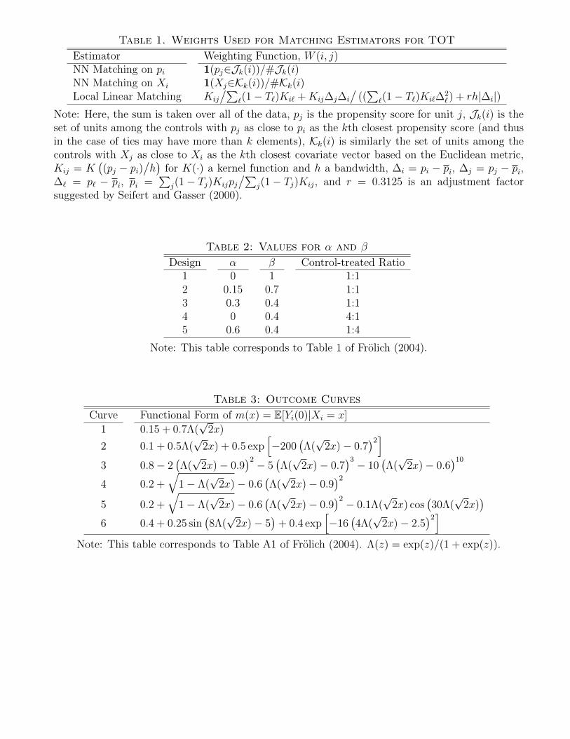
Table 1. Weights Used for Matching Estimators for TOT

Estimator Weighting Function, W (i, j)NN Matching on pi 1(pj∈Jk(i))/#Jk(i)NN Matching on Xi 1(Xj∈Kk(i))/#Kk(i)Local Linear Matching Kij

/∑`(1− T`)Ki` +Kij∆j∆i

/((∑

`(1− T`)Ki`∆2`) + rh|∆i|)

Note: Here, the sum is taken over all of the data, pj is the propensity score for unit j, Jk(i) is theset of units among the controls with pj as close to pi as the kth closest propensity score (and thusin the case of ties may have more than k elements), Kk(i) is similarly the set of units among thecontrols with Xj as close to Xi as the kth closest covariate vector based on the Euclidean metric,Kij = K

((pj − pi)

/h)

for K(·) a kernel function and h a bandwidth, ∆i = pi − pi, ∆j = pj − pi,∆` = p` − pi, pi =

∑j(1− Tj)Kijpj

/∑j(1− Tj)Kij, and r = 0.3125 is an adjustment factor

suggested by Seifert and Gasser (2000).

Table 2: Values for α and β

Design α β Control-treated Ratio1 0 1 1:12 0.15 0.7 1:13 0.3 0.4 1:14 0 0.4 4:15 0.6 0.4 1:4

Note: This table corresponds to Table 1 of Frolich (2004).

Table 3: Outcome Curves

Curve Functional Form of m(x) = E[Yi(0)|Xi = x]

1 0.15 + 0.7Λ(√

2x)

2 0.1 + 0.5Λ(√

2x) + 0.5 exp[−200

(Λ(√

2x)− 0.7)2]

3 0.8− 2(Λ(√

2x)− 0.9)2 − 5

(Λ(√

2x)− 0.7)3 − 10

(Λ(√

2x)− 0.6)10

4 0.2 +√

1− Λ(√

2x)− 0.6(Λ(√

2x)− 0.9)2

5 0.2 +√

1− Λ(√

2x)− 0.6(Λ(√

2x)− 0.9)2 − 0.1Λ(

√2x) cos

(30Λ(

√2x))

6 0.4 + 0.25 sin(8Λ(√

2x)− 5)

+ 0.4 exp[−16

(4Λ(√

2x)− 2.5)2]

Note: This table corresponds to Table A1 of Frolich (2004). Λ(z) = exp(z)/(1 + exp(z)).

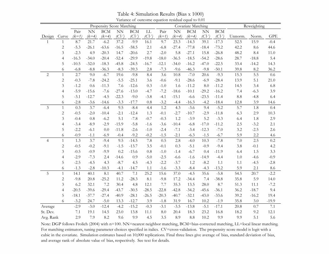
Table 4: Simulation Results (Bias x 1000)Variance of outcome equation residual equal to 0.01

Propensity Score Matching Covariate Matching ReweightingPair NN BCM NN BCM LL Pair NN BCM NN BCM

Design Curve (k=1) (k=4) (k=4) (CV) (CV) (CV) (k=1) (k=4) (k=4) (CV) (CV) Unnorm. Norm. GPE1 1 8.7 21.7 -6.2 37.2 -9.9 16.1 9.7 23.3 -14.3 39.1 -17.3 52.5 15.9 -0.4

2 -5.3 -26.1 -63.6 -16.5 -58.5 2.1 -6.8 -27.4 -77.8 -18.4 -73.2 42.2 8.6 44.63 -2.3 4.9 -20.3 14.7 -20.6 2.7 -2.0 5.8 -27.1 15.8 -26.8 48.2 8.4 11.04 -16.3 -34.0 -20.4 -52.4 -29.9 -19.8 -18.0 -36.5 -18.5 -54.2 -28.6 28.7 -18.8 5.45 -10.5 -32.0 -18.3 -45.8 -24.5 -16.7 -12.1 -34.0 -16.2 -47.0 -22.5 33.4 -14.2 14.36 -6.8 -8.8 -36.3 -8.3 -39.3 2.8 -7.3 -9.6 -46.3 -9.8 -50.1 39.8 8.2 36.2

2 1 2.7 9.0 -6.7 19.6 -9.8 8.4 3.6 10.8 -7.0 20.6 -9.3 15.3 5.5 0.62 -0.3 -7.8 -24.2 -5.5 -25.1 3.6 -0.6 -9.1 -28.6 -6.9 -28.4 13.9 5.1 21.03 -1.2 0.6 -11.3 7.6 -12.6 0.3 -1.0 1.6 -11.2 8.0 -11.2 14.5 3.4 6.84 -5.9 -15.6 -7.6 -27.6 -13.0 -4.7 -7.2 -18.6 -10.1 -29.2 -16.2 7.4 -6.3 3.95 -3.1 -12.7 -4.5 -22.3 -9.0 -3.8 -4.1 -15.1 -6.6 -23.5 -11.4 8.8 -4.8 6.46 -2.8 -3.6 -14.6 -3.3 -17.7 0.8 -3.2 -4.4 -16.3 -4.2 -18.4 12.8 3.9 14.6

3 1 0.3 3.7 -6.4 9.5 -8.4 4.4 1.2 4.3 -3.6 9.4 -5.2 5.7 1.8 0.42 -0.5 -2.0 -10.4 -2.1 -12.4 1.3 -0.1 -2.7 -10.7 -2.9 -11.8 6.3 2.9 10.33 -0.4 0.8 -6.2 5.1 -7.8 -0.7 -0.3 1.2 -3.9 5.2 -3.3 6.4 1.8 2.94 -3.4 -8.9 -2.9 -15.9 -5.8 -1.6 -3.6 -10.4 -6.8 -17.0 -11.2 2.5 -3.2 2.15 -2.2 -6.1 0.0 -11.8 -2.6 -1.0 -2.4 -7.1 -3.4 -12.3 -7.0 3.2 -2.5 2.66 -0.9 -1.1 -6.9 -0.4 -9.2 -0.2 -1.5 -2.1 -6.3 -1.5 -6.7 5.9 2.2 4.6

4 1 1.3 3.7 -9.4 9.5 -14.5 7.8 0.5 2.8 -4.0 10.3 -7.8 7.0 2.5 0.22 -0.5 -0.2 -9.1 -1.5 -13.7 3.5 -0.1 0.3 -5.1 -0.9 -9.4 3.8 -0.1 4.23 -0.5 -0.9 -9.9 0.2 -15.6 0.8 -1.0 -1.4 -6.7 0.4 -11.9 6.4 1.5 3.34 -2.9 -7.3 2.4 -14.6 0.9 -5.0 -2.5 -6.6 -1.6 -14.9 -4.4 1.0 -4.6 -0.95 -2.5 -4.5 4.3 -8.7 4.5 -4.3 -2.2 -3.7 1.2 -8.2 1.1 1.1 -4.5 -2.86 -1.3 -2.8 -10.3 -4.1 -14.7 1.1 -1.6 -3.3 -8.4 -4.3 -13.2 5.9 2.1 8.6

5 1 14.1 40.1 8.1 40.7 7.1 25.2 15.6 37.0 -4.5 35.6 -5.8 54.5 20.7 -2.22 -9.8 20.8 -25.2 11.2 -28.3 8.1 -9.8 17.2 -34.4 7.4 -38.8 35.8 5.9 14.03 6.2 32.1 7.2 30.4 4.8 12.1 7.7 35.3 13.5 28.0 8.7 51.3 11.1 -7.24 -20.5 -39.6 -29.4 -43.7 -30.5 -28.5 -22.8 -42.8 -34.2 -45.6 -36.1 36.2 -18.7 9.45 -18.1 -37.7 -27.4 -40.9 -28.1 -26.5 -20.3 -40.7 -32.1 -43.0 -33.6 39.2 -16.2 19.46 -3.2 24.7 -5.0 13.3 -12.7 3.9 -1.8 31.9 16.7 10.2 -1.9 35.8 3.0 -19.9

Average -2.9 -3.0 -12.4 -4.2 -15.2 -0.3 -3.1 -3.5 -13.8 -5.1 -17.1 20.8 0.7 7.1St. Dev. 7.1 19.1 14.5 23.0 13.8 11.1 8.0 20.4 18.3 23.2 16.8 18.2 9.2 12.1Avg. Rank 2.9 7.9 8.2 9.6 9.9 4.5 3.5 8.9 8.8 10.2 9.9 9.9 5.1 5.6

Note: DGP follows Frolich (2004) with n=100. NN=nearest neighbor matching, BCM=bias-corrected matching, LL=local linear matching. For matching estimators, tuning parameter choices specified in italics. CV=cross-validation. The propensity score model is logit with a cubic in the covariate. Simulation estimates based on 10,000 replications. Final three lines give average of bias, standard deviation of bias, and average rank of absolute value of bias, respectively. See text for details.

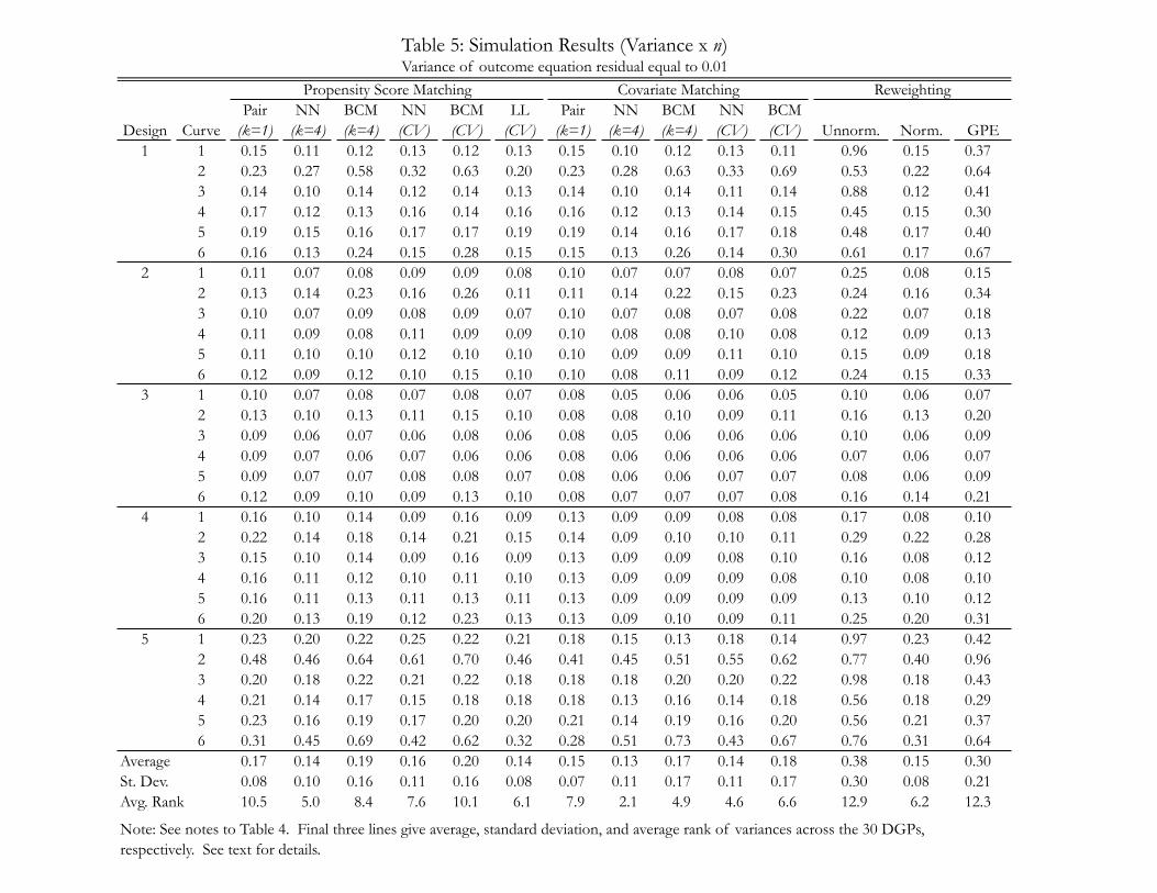
Table 5: Simulation Results (Variance x n)Variance of outcome equation residual equal to 0.01

Propensity Score Matching Covariate Matching ReweightingPair NN BCM NN BCM LL Pair NN BCM NN BCM

Design Curve (k=1) (k=4) (k=4) (CV) (CV) (CV) (k=1) (k=4) (k=4) (CV) (CV) Unnorm. Norm. GPE1 1 0.15 0.11 0.12 0.13 0.12 0.13 0.15 0.10 0.12 0.13 0.11 0.96 0.15 0.37

2 0.23 0.27 0.58 0.32 0.63 0.20 0.23 0.28 0.63 0.33 0.69 0.53 0.22 0.643 0.14 0.10 0.14 0.12 0.14 0.13 0.14 0.10 0.14 0.11 0.14 0.88 0.12 0.414 0.17 0.12 0.13 0.16 0.14 0.16 0.16 0.12 0.13 0.14 0.15 0.45 0.15 0.305 0.19 0.15 0.16 0.17 0.17 0.19 0.19 0.14 0.16 0.17 0.18 0.48 0.17 0.406 0.16 0.13 0.24 0.15 0.28 0.15 0.15 0.13 0.26 0.14 0.30 0.61 0.17 0.67

2 1 0.11 0.07 0.08 0.09 0.09 0.08 0.10 0.07 0.07 0.08 0.07 0.25 0.08 0.152 0.13 0.14 0.23 0.16 0.26 0.11 0.11 0.14 0.22 0.15 0.23 0.24 0.16 0.343 0.10 0.07 0.09 0.08 0.09 0.07 0.10 0.07 0.08 0.07 0.08 0.22 0.07 0.184 0.11 0.09 0.08 0.11 0.09 0.09 0.10 0.08 0.08 0.10 0.08 0.12 0.09 0.135 0.11 0.10 0.10 0.12 0.10 0.10 0.10 0.09 0.09 0.11 0.10 0.15 0.09 0.186 0.12 0.09 0.12 0.10 0.15 0.10 0.10 0.08 0.11 0.09 0.12 0.24 0.15 0.33

3 1 0.10 0.07 0.08 0.07 0.08 0.07 0.08 0.05 0.06 0.06 0.05 0.10 0.06 0.072 0.13 0.10 0.13 0.11 0.15 0.10 0.08 0.08 0.10 0.09 0.11 0.16 0.13 0.203 0.09 0.06 0.07 0.06 0.08 0.06 0.08 0.05 0.06 0.06 0.06 0.10 0.06 0.094 0.09 0.07 0.06 0.07 0.06 0.06 0.08 0.06 0.06 0.06 0.06 0.07 0.06 0.075 0.09 0.07 0.07 0.08 0.08 0.07 0.08 0.06 0.06 0.07 0.07 0.08 0.06 0.096 0.12 0.09 0.10 0.09 0.13 0.10 0.08 0.07 0.07 0.07 0.08 0.16 0.14 0.21

4 1 0.16 0.10 0.14 0.09 0.16 0.09 0.13 0.09 0.09 0.08 0.08 0.17 0.08 0.102 0.22 0.14 0.18 0.14 0.21 0.15 0.14 0.09 0.10 0.10 0.11 0.29 0.22 0.283 0.15 0.10 0.14 0.09 0.16 0.09 0.13 0.09 0.09 0.08 0.10 0.16 0.08 0.124 0.16 0.11 0.12 0.10 0.11 0.10 0.13 0.09 0.09 0.09 0.08 0.10 0.08 0.105 0.16 0.11 0.13 0.11 0.13 0.11 0.13 0.09 0.09 0.09 0.09 0.13 0.10 0.126 0.20 0.13 0.19 0.12 0.23 0.13 0.13 0.09 0.10 0.09 0.11 0.25 0.20 0.31

5 1 0.23 0.20 0.22 0.25 0.22 0.21 0.18 0.15 0.13 0.18 0.14 0.97 0.23 0.422 0.48 0.46 0.64 0.61 0.70 0.46 0.41 0.45 0.51 0.55 0.62 0.77 0.40 0.963 0.20 0.18 0.22 0.21 0.22 0.18 0.18 0.18 0.20 0.20 0.22 0.98 0.18 0.434 0.21 0.14 0.17 0.15 0.18 0.18 0.18 0.13 0.16 0.14 0.18 0.56 0.18 0.295 0.23 0.16 0.19 0.17 0.20 0.20 0.21 0.14 0.19 0.16 0.20 0.56 0.21 0.376 0.31 0.45 0.69 0.42 0.62 0.32 0.28 0.51 0.73 0.43 0.67 0.76 0.31 0.64

Average 0.17 0.14 0.19 0.16 0.20 0.14 0.15 0.13 0.17 0.14 0.18 0.38 0.15 0.30St. Dev. 0.08 0.10 0.16 0.11 0.16 0.08 0.07 0.11 0.17 0.11 0.17 0.30 0.08 0.21Avg. Rank 10.5 5.0 8.4 7.6 10.1 6.1 7.9 2.1 4.9 4.6 6.6 12.9 6.2 12.3

Note: See notes to Table 4. Final three lines give average, standard deviation, and average rank of variances across the 30 DGPs, respectively. See text for details.

Table 6: Simulation Results (Bias x 1000)Variance of outcome equation residual equal to 0.10

Propensity Score Matching Covariate Matching ReweightingPair NN BCM NN BCM LL Pair NN BCM NN BCM

Design Curve (k=1) (k=4) (k=4) (CV) (CV) (CV) (k=1) (k=4) (k=4) (CV) (CV) Unnorm. Norm. GPE1 1 9.1 21.2 -6.8 64.8 -11.3 18.9 10.1 22.8 -15.0 65.7 -18.1 52.3 15.7 -1.0

2 -4.9 -26.6 -64.2 21.3 -66.9 0.1 -6.5 -28.0 -78.5 21.7 -76.2 41.9 8.3 44.03 -1.9 4.4 -20.9 47.0 -9.8 8.2 -1.7 5.2 -27.8 48.6 -15.1 47.9 8.2 10.44 -15.9 -34.6 -21.0 -68.5 -40.3 -36.5 -17.6 -37.0 -19.2 -69.7 -39.4 28.4 -19.0 4.95 -10.1 -32.5 -18.9 -64.7 -36.4 -32.2 -11.7 -34.6 -16.9 -65.9 -35.3 33.2 -14.5 13.76 -6.4 -9.3 -36.8 16.2 -37.7 -2.6 -6.9 -10.2 -47.0 16.4 -47.0 39.5 7.9 35.5

2 1 3.2 9.2 -6.5 38.2 -11.2 10.1 3.9 10.8 -7.0 39.8 -9.9 15.5 5.7 0.82 0.2 -7.6 -24.0 9.9 -39.1 4.9 -0.3 -9.1 -28.6 9.5 -40.9 14.1 5.3 21.23 -0.7 0.8 -11.2 28.5 -7.0 2.7 -0.7 1.6 -11.2 31.4 -2.5 14.7 3.6 6.94 -5.4 -15.5 -7.4 -42.3 -19.2 -15.6 -6.9 -18.6 -10.1 -45.3 -22.9 7.6 -6.1 4.15 -2.7 -12.6 -4.3 -39.8 -16.6 -13.5 -3.8 -15.1 -6.6 -42.5 -20.5 9.0 -4.6 6.56 -2.4 -3.4 -14.4 8.0 -18.5 -2.4 -2.9 -4.3 -16.3 9.4 -16.6 13.0 4.1 14.8

3 1 -0.4 3.2 -7.0 18.5 -10.0 3.9 1.0 3.7 -4.2 18.3 -6.8 5.0 1.0 -0.52 -1.1 -2.5 -11.0 2.3 -22.6 1.9 -0.3 -3.3 -11.3 -0.1 -23.8 5.6 2.2 9.43 -1.0 0.2 -6.8 16.3 -5.5 -0.7 -0.5 0.7 -4.4 19.2 2.3 5.6 1.1 2.04 -4.0 -9.4 -3.5 -26.6 -10.3 -7.7 -3.9 -11.0 -7.4 -30.1 -18.0 1.8 -3.9 1.25 -2.8 -6.7 -0.6 -24.8 -8.4 -6.7 -2.6 -7.7 -4.0 -27.8 -15.8 2.4 -3.3 1.86 -1.6 -1.6 -7.5 4.7 -11.2 -3.5 -1.8 -2.7 -6.9 5.0 -5.6 5.1 1.4 3.7

4 1 1.2 3.8 -9.3 19.6 -17.9 8.0 -0.2 2.7 -4.1 22.0 -10.1 7.1 2.6 0.02 -0.6 -0.1 -9.0 -3.1 -29.2 4.4 -0.7 0.1 -5.2 -3.2 -26.0 3.9 0.1 3.93 -0.6 -0.8 -9.8 8.8 -18.8 -0.1 -1.7 -1.6 -6.9 12.7 -13.5 6.5 1.6 3.14 -3.0 -7.1 2.4 -27.2 -2.7 -8.5 -3.2 -6.8 -1.8 -30.8 -8.9 1.1 -4.5 -1.15 -2.6 -4.4 4.3 -24.0 -0.2 -7.7 -2.9 -3.8 1.0 -27.1 -5.8 1.2 -4.4 -3.06 -1.4 -2.7 -10.3 -4.2 -21.7 -1.6 -2.3 -3.5 -8.6 -2.1 -20.2 6.0 2.2 8.4

5 1 14.9 40.5 8.7 63.8 10.6 38.1 16.5 37.5 -3.6 58.1 -2.5 55.7 21.9 -1.22 -9.0 21.2 -24.7 49.2 -17.1 18.6 -9.0 17.7 -33.5 44.3 -23.7 37.0 7.2 15.03 7.0 32.5 7.7 51.4 15.1 25.0 8.5 35.9 14.4 54.1 26.9 52.5 12.4 -6.24 -19.7 -39.2 -28.8 -47.2 -32.0 -31.1 -21.9 -42.2 -33.4 -49.8 -37.9 37.4 -17.5 10.45 -17.3 -37.3 -26.8 -45.3 -30.0 -29.0 -19.5 -40.1 -31.2 -47.7 -35.6 40.4 -14.9 20.46 -2.5 25.1 -4.5 39.8 5.6 10.1 -0.9 32.5 17.5 43.8 32.0 37.1 4.2 -18.9

Average -2.7 -3.1 -12.4 3.0 -17.3 -1.5 -3.0 -3.6 -13.9 2.6 -17.9 20.9 0.8 7.0St. Dev. 7.0 19.2 14.6 37.3 16.9 16.6 7.9 20.5 18.4 38.4 20.7 18.5 9.2 12.0Avg. Rank 2.7 6.8 7.6 11.3 9.8 6.6 3.4 7.8 8.3 11.7 10.6 8.9 4.5 5.0

Note: See notes to Table 4. Final three lines give average of bias, standard deviation of bias, and average rank of absolute value of bias across 30 DGPs, respectively. See text for details.

Table 7: Simulation Results (Variance x n)Variance of outcome equation residual equal to 0.10

Propensity Score Matching Covariate Matching ReweightingPair NN BCM NN BCM LL Pair NN BCM NN BCM

Design Curve (k=1) (k=4) (k=4) (CV) (CV) (CV) (k=1) (k=4) (k=4) (CV) (CV) Unnorm. Norm. GPE1 1 1.41 0.88 1.13 1.07 1.05 0.96 1.39 0.87 1.22 1.05 1.09 1.86 0.99 2.74

2 1.51 1.05 1.77 1.36 1.82 1.21 1.49 1.06 2.02 1.38 1.92 1.67 1.12 3.353 1.40 0.87 1.17 0.99 1.11 1.11 1.39 0.86 1.26 0.98 1.15 1.82 0.96 2.754 1.44 0.90 1.10 0.82 0.96 0.99 1.41 0.89 1.13 0.82 0.99 1.56 1.00 2.755 1.47 0.93 1.13 0.83 0.99 1.01 1.45 0.92 1.17 0.83 1.02 1.60 1.02 2.886 1.41 0.90 1.29 1.09 1.45 1.08 1.38 0.89 1.42 1.10 1.57 1.61 1.03 3.20

2 1 0.98 0.65 0.73 0.73 0.71 0.65 0.95 0.64 0.71 0.71 0.66 0.81 0.64 1.242 1.00 0.72 0.90 0.83 1.06 0.76 0.97 0.71 0.90 0.83 1.01 0.84 0.74 1.513 0.97 0.65 0.74 0.68 0.71 0.70 0.95 0.63 0.72 0.68 0.68 0.78 0.63 1.264 0.99 0.66 0.72 0.65 0.66 0.69 0.96 0.65 0.70 0.65 0.65 0.73 0.65 1.245 0.99 0.67 0.74 0.66 0.68 0.70 0.96 0.66 0.72 0.66 0.67 0.75 0.65 1.296 0.99 0.67 0.77 0.71 0.85 0.72 0.96 0.65 0.75 0.71 0.81 0.81 0.72 1.44

3 1 0.80 0.54 0.58 0.56 0.56 0.52 0.77 0.52 0.54 0.53 0.51 0.53 0.48 0.642 0.83 0.58 0.63 0.62 0.74 0.59 0.78 0.55 0.59 0.60 0.68 0.60 0.57 0.783 0.80 0.54 0.58 0.54 0.56 0.52 0.77 0.52 0.55 0.53 0.53 0.53 0.49 0.664 0.80 0.54 0.56 0.53 0.52 0.52 0.77 0.53 0.54 0.53 0.51 0.51 0.49 0.665 0.80 0.55 0.57 0.53 0.54 0.53 0.77 0.53 0.55 0.53 0.52 0.52 0.50 0.676 0.82 0.56 0.60 0.58 0.66 0.57 0.77 0.53 0.56 0.55 0.58 0.59 0.57 0.78

4 1 1.35 0.88 0.98 0.82 0.95 0.79 1.31 0.85 0.87 0.80 0.78 0.86 0.76 0.932 1.41 0.93 1.02 0.88 1.14 0.89 1.32 0.87 0.88 0.85 0.96 0.98 0.90 1.123 1.34 0.88 0.97 0.80 0.95 0.80 1.31 0.86 0.88 0.79 0.82 0.85 0.76 0.944 1.34 0.89 0.96 0.83 0.84 0.81 1.32 0.86 0.87 0.83 0.77 0.79 0.76 0.925 1.35 0.90 0.97 0.84 0.87 0.83 1.32 0.86 0.88 0.83 0.79 0.82 0.78 0.946 1.39 0.91 1.03 0.83 1.09 0.85 1.31 0.86 0.88 0.79 0.88 0.94 0.88 1.14

5 1 1.67 1.12 1.44 1.28 1.41 1.31 1.55 1.03 1.38 1.18 1.34 1.98 1.23 2.842 1.93 1.40 1.94 1.72 1.93 1.65 1.81 1.34 1.83 1.61 1.79 1.79 1.40 3.283 1.66 1.09 1.44 1.11 1.43 1.19 1.57 1.06 1.37 1.13 1.38 1.98 1.20 2.864 1.63 1.06 1.35 0.95 1.29 1.08 1.54 1.02 1.32 0.94 1.27 1.89 1.19 2.765 1.66 1.07 1.36 0.96 1.30 1.09 1.56 1.04 1.34 0.95 1.29 1.89 1.22 2.906 1.78 1.38 1.94 1.42 2.02 1.40 1.69 1.42 1.91 1.53 2.09 1.73 1.33 3.10

Average 1.26 0.85 1.04 0.87 1.03 0.88 1.22 0.82 1.01 0.86 0.99 1.15 0.85 1.79St. Dev. 0.34 0.23 0.39 0.29 0.41 0.29 0.32 0.23 0.42 0.28 0.43 0.54 0.27 1.00Avg. Rank 12.6 5.0 10.1 5.0 8.9 4.7 11.4 3.0 8.4 4.1 6.5 9.0 3.2 13.0

Note: See notes to Table 4. Final three lines give average, standard deviation, and average rank of variances across the 30 DGPs, respectively. See text for details.

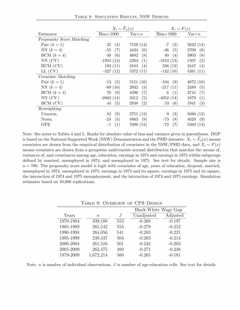
Table 8: Simulation Results, NSW Designs

Xi ∼ Fn(x) Xi ∼ F (x)Estimator Bias×1000 Var×n Bias×1000 Var×nPropensity Score Matching

Pair (k = 1) 35 (4) 7150 (14) -7 (2) 5632 (14)NN (k = 4) -55 (7) 4434 (6) -46 (5) 3709 (6)BCM (k = 4) 49 (6) 4682 (8) 40 (4) 3903 (8)NN (CV ) -1924 (13) 2263 (1) -1853 (13) 1507 (2)BCM (CV ) 193 (11) 3184 (4) 338 (12) 2447 (4)LL (CV ) -327 (12) 5372 (11) -132 (10) 4381 (11)

Covariate MatchingPair (k = 1) -13 (2) 5151 (10) -104 (9) 4072 (10)NN (k = 4) -89 (10) 2932 (3) -217 (11) 2489 (5)BCM (k = 4) 70 (8) 4596 (7) 6 (1) 3745 (7)NN (CV ) -2803 (14) 3312 (5) -4052 (14) 1079 (1)BCM (CV ) 44 (5) 2838 (2) 53 (6) 1941 (3)

ReweightingUnnorm. 82 (9) 5751 (12) 9 (3) 5086 (12)Norm. -24 (3) 4863 (9) -73 (8) 4029 (9)GPE -1 (1) 7098 (13) -72 (7) 5569 (13)

Note: See notes to Tables 4 and 5. Ranks for absolute value of bias and variance given in parentheses. DGPis based on the National Supported Work (NSW) Demonstration and the PSID datasets. Xi ∼ Fn(x) meanscovariates are drawn from the empirical distribution of covariates in the NSW/PSID data, and Xi ∼ F (x)means covariates are drawn from a groupwise multivariate normal distribution that matches the means of,variances of, and covariances among age, education, earnings in 1974 and earnings in 1975 within subgroupsdefined by married, unemployed in 1974, and unemployed in 1975. See text for details. Sample size isn = 780. The propensity score model is logit with covariates of age, years of education, dropout, married,unemployed in 1974, unemployed in 1975, earnings in 1974 and its square, earnings in 1975 and its square,the interaction of 1974 and 1975 unemployment, and the interaction of 1974 and 1975 earnings. Simulationestimates based on 10,000 replications.

Table 9: Overview of CPS Design

Black-White Wage GapYears n J Unadjusted Adjusted

1979-1984 339,188 553 -0.268 -0.1971985-1989 285,542 553 -0.279 -0.2121990-1994 284,056 541 -0.283 -0.2211995-1999 239,437 504 -0.263 -0.2142000-2004 261,516 501 -0.242 -0.2032005-2009 262,475 493 -0.271 -0.2381979-2009 1,672,214 560 -0.265 -0.181

Note: n is number of individual observations, J is number of age-education cells. See text for details.

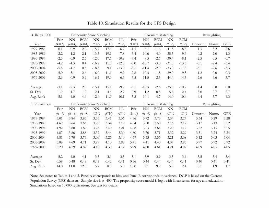
Table 10: Simulation Results for the CPS Design

A. Bias x 1000 Propensity Score Matching Covariate Matching ReweightingPair NN BCM NN BCM LL Pair NN BCM NN BCM

Year (k=1) (k=4) (k=4) (CV) (CV) (CV) (k=1) (k=4) (k=4) (CV) (CV) Unnorm. Norm. GPE1979-1984 0.1 -0.9 2.2 -15.7 17.6 -6.7 -1.5 -8.1 -1.6 -41.5 -8.8 1.3 3.2 2.61985-1989 -2.2 -1.2 2.1 -13.3 19.1 -7.8 -3.4 -10.6 -4.0 -35.5 -9.6 0.2 2.0 1.31990-1994 -2.3 -0.9 2.5 -12.0 17.7 -10.8 -4.4 -9.5 -2.7 -30.4 -8.1 -2.5 0.5 -0.71995-1999 -4.2 -4.3 0.4 -16.2 11.3 -12.8 -3.0 -10.7 -3.0 -31.3 -13.3 -5.1 -2.4 -3.42000-2004 -5.5 -4.7 0.5 -18.3 9.1 -13.0 -3.1 -11.4 -2.9 -33.0 -11.8 -5.1 -2.6 -3.32005-2009 -5.0 -3.1 2.6 -16.0 11.1 -9.9 -2.8 -10.3 -1.8 -29.0 -9.3 -1.2 0.0 -0.31979-2009 -2.6 -0.9 3.9 -16.2 19.6 -6.6 -3.5 -11.5 -2.5 -44.4 -14.5 2.6 4.6 3.7

Average -3.1 -2.3 2.0 -15.4 15.1 -9.7 -3.1 -10.3 -2.6 -35.0 -10.7 -1.4 0.8 0.0St. Dev. 1.9 1.7 1.2 2.1 4.4 2.7 0.9 1.2 0.8 5.8 2.4 3.0 2.7 2.7Avg. Rank 5.1 4.0 4.4 12.4 11.9 10.1 5.3 10.1 4.7 14.0 10.4 4.4 3.7 4.3

B. Variance x n Propensity Score Matching Covariate Matching ReweightingPair NN BCM NN BCM LL Pair NN BCM NN BCM

Year (k=1) (k=4) (k=4) (CV) (CV) (CV) (k=1) (k=4) (k=4) (CV) (CV) Unnorm. Norm. GPE1979-1984 5.01 3.84 3.85 3.33 3.41 3.36 4.96 3.72 3.73 3.34 3.24 3.34 3.29 3.281985-1989 4.69 3.64 3.66 3.20 3.34 3.19 4.54 3.50 3.50 3.16 3.12 3.17 3.13 3.121990-1994 4.92 3.80 3.82 3.25 3.40 3.21 4.68 3.63 3.64 3.20 3.19 3.22 3.15 3.151995-1999 4.87 3.86 3.88 3.32 3.44 3.30 4.80 3.70 3.71 3.32 3.29 3.31 3.24 3.242000-2004 4.81 3.70 3.73 3.09 3.25 3.10 4.69 3.53 3.55 3.21 3.08 3.12 3.03 3.042005-2009 5.88 4.69 4.71 3.99 4.10 3.98 5.71 4.41 4.40 4.07 3.95 3.97 3.92 3.921979-2009 6.20 4.79 4.82 4.18 4.30 4.12 5.99 4.60 4.61 4.21 4.07 4.09 4.05 4.05

Average 5.2 4.0 4.1 3.5 3.6 3.5 5.1 3.9 3.9 3.5 3.4 3.5 3.4 3.4St. Dev. 0.59 0.48 0.48 0.42 0.42 0.41 0.56 0.44 0.44 0.44 0.41 0.40 0.41 0.41Avg. Rank 14.0 11.0 12.0 5.7 8.0 5.3 13.0 9.1 9.9 5.9 2.4 5.1 1.9 1.7

Note: See notes to Tables 4 and 5. Panel A corresponds to bias, and Panel B corresponds to variance. DGP is based on the CurrentPopulation Survey (CPS) datasets. Sample size is n=400. The propensity score model is logit with linear terms for age and education. Simulations based on 10,000 replications. See text for details.

Table 11: The Role of Overlap in the NSW and CPS Designs

Propensity Score Matching Covariate Matching ReweightingPair NN BCM NN BCM LL Pair NN BCM NN BCM

(k=1) (k=4) (k=4) (CV) (CV) (CV) (k=1) (k=4) (k=4) (CV) (CV) Unnorm. Norm. GPEA. NSW: Covariates Drawn from Empirical Distribution

Bad Overlap Bias x 1000 35 -55 49 -1924 193 -327 -13 -89 70 -2803 44 82 -24 -1(4) (7) (6) (13) (11) (12) (2) (10) (8) (14) (5) (9) (3) (1)

Variance x n 7150 4434 4682 2263 3184 5372 5151 2932 4596 3312 2838 5751 4863 7098(14) (6) (8) (1) (4) (11) (10) (3) (7) (5) (2) (12) (9) (13)

Medium Overlap Bias x 1000 41 63 91 -302 357 -103 65 130 117 -558 146 14 11 3(4) (5) (7) (12) (13) (8) (6) (10) (9) (14) (11) (3) (2) (1)

Variance x n 1201 971 978 891 913 923 1062 905 868 1159 804 837 837 809(14) (10) (11) (6) (8) (9) (12) (7) (5) (13) (1) (3) (4) (2)

Good Overlap Bias x 1000 84 123 132 97 190 4 123 252 121 97 121 11 9 1(5) (11) (12) (7) (13) (2) (10) (14) (9) (6) (8) (4) (3) (1)

Variance x n 1064 825 826 754 768 759 853 733 691 814 645 661 657 644(14) (11) (12) (7) (9) (8) (13) (6) (5) (10) (2) (4) (3) (1)

B. NSW: Covariates Drawn from Matched-Moments DistributionBad Overlap Bias x 1000 -7 -46 40 -1853 338 -132 -104 -217 6 -4052 53 9 -73 -72

(2) (5) (4) (13) (12) (10) (9) (11) (1) (14) (6) (3) (8) (7)Variance x n 5632 3709 3903 1507 2447 4381 4072 2489 3745 1079 1941 5086 4029 5569

(14) (6) (8) (2) (4) (11) (10) (5) (7) (1) (3) (12) (9) (13)

Medium Overlap Bias x 1000 27 10 37 -411 372 -120 65 41 92 -1291 79 -6 -8 -8(5) (4) (6) (13) (12) (11) (8) (7) (10) (14) (9) (1) (3) (2)

Variance x n 972 687 690 594 625 676 829 653 638 790 555 585 589 580(14) (10) (11) (5) (6) (9) (13) (8) (7) (12) (1) (3) (4) (2)

Good Overlap Bias x 1000 156 110 116 37 145 19 155 188 111 -279 96 13 12 10(12) (7) (9) (5) (10) (4) (11) (13) (8) (14) (6) (3) (2) (1)

Variance x n 920 620 619 578 579 594 685 566 540 655 491 497 497 495(14) (11) (10) (7) (8) (9) (13) (6) (5) (12) (1) (4) (3) (2)

C. CPSBad Overlap Bias x 1000 -9.3 -19.8 -4.8 -69.4 14.3 -13.7 -7.6 -19.0 0.5 -101.5 -14.3 6.6 1.3 4.0

(7) (12) (4) (13) (9) (8) (6) (11) (1) (14) (10) (5) (2) (3)Variance x n 5.93 4.59 4.98 3.71 4.19 4.34 5.53 4.27 4.56 4.01 3.76 12.03 4.86 4.45

(13) (9) (11) (1) (4) (6) (12) (5) (8) (3) (2) (14) (10) (7)

Medium Overlap Bias x 1000 -7.6 -12.5 -5.8 -39.0 10.8 -6.6 -2.9 -9.9 -1.5 -60.5 -14.0 0.3 2.2 2.2(8) (11) (6) (13) (10) (7) (5) (9) (2) (14) (12) (1) (4) (3)

Variance x n 4.72 3.77 3.81 3.25 3.31 3.31 4.67 3.64 3.67 3.41 3.21 3.59 3.32 3.27(14) (11) (12) (2) (4) (5) (13) (9) (10) (7) (1) (8) (6) (3)

Good Overlap Bias x 1000 0.1 -0.9 2.2 -15.7 17.6 -6.7 -1.5 -8.1 -1.6 -41.5 -8.8 1.3 3.2 2.6(1) (2) (6) (12) (13) (9) (4) (10) (5) (14) (11) (3) (8) (7)

Variance x n 5.01 3.84 3.85 3.33 3.41 3.36 4.96 3.72 3.73 3.34 3.24 3.34 3.29 3.28(14) (11) (12) (4) (8) (7) (13) (9) (10) (5) (1) (6) (3) (2)

Note: See notes to Tables 4, 8, and 9. See text for details.

Figure 1: Overlap Plots for Designs 1 through 5

0.5

11.5

2

0 .2 .4 .6 .8 1

A. Design 1

0.5

11.5

22.5

.1 .3 .5 .7 .9

B. Design 20

12

34

.3 .4 .5 .6 .7

C. Design 3

01

23

4

0 .1 .2 .3 .4

D. Design 4

01

23

4

.6 .7 .8 .9 1

E. Design 5

Note: Solid lines give density function for propensity score conditional on Ti = 1. Dashed lines givedensity function for propensity score conditional on Ti = 0. See text for details.

Figure 2: Conditional Expectations for Curves 1 through 6

0.2

.4.6

.81

−4 −2 0 2 4

A. Curve 1

0.2

.4.6

.81

−4 −2 0 2 4

B. Curve 20

.2.4

.6.8

1

−4 −2 0 2 4

C. Curve 3

0.2

.4.6

.81

−4 −2 0 2 4

D. Curve 4

0.2

.4.6

.81

−4 −2 0 2 4

E. Curve 5

0.2

.4.6

.81

−4 −2 0 2 4

F. Curve 6

Note: Each panel displays the conditional expectation of Yi(0) given Xi = x for the curve inquestion. See text for details.

Figure 3: Overlap Plots for the NSW Design

05

1015

20D

ensi

ty o

f Pro

pens

ity S

core

Giv

en T

reat

men

t

0 .2 .4 .6 .8 1Propensity Score

A. Covariates Drawn from Empirical Distribution

05

1015

20D

ensi

ty o

f Pro

pens

ity S

core

Giv

en T

reat

men

t

0 .2 .4 .6 .8 1Propensity Score

B. Covariates Drawn from Matched−Moments Distribution

Note: Panel A displays an overlap plot for the NSW Design where Xi is drawn from the empiricaldistribution of covariates in the NSW/PSID data. Panel B displays an overlap plot for the NSWDesign where Xi is drawn from a mixed discrete-continuous distribution that is groupwise multi-variate normal. Solid line is a kernel density estimate of the conditional density of the propensityscore among treated units for a representative data set. Dashed line is for the conditional densityamong control units. Solid triangles at top of figure give propensity score values for treated units,and open circles at bottom of figure give propensity score values for control units. See text fordetails.

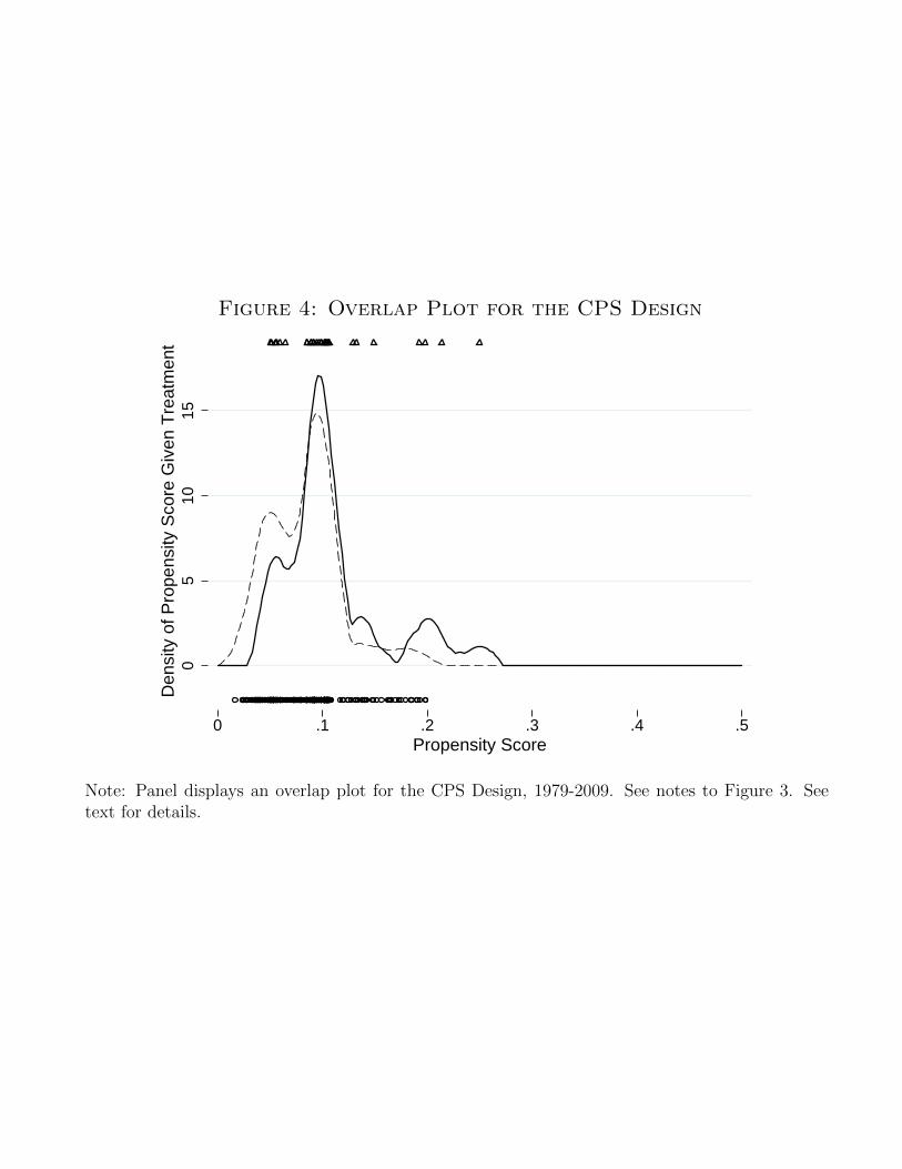
Figure 4: Overlap Plot for the CPS Design

05

1015

Den

sity

of P

rope

nsity

Sco

re G

iven

Tre

atm

ent

0 .1 .2 .3 .4 .5Propensity Score

Note: Panel displays an overlap plot for the CPS Design, 1979-2009. See notes to Figure 3. Seetext for details.