Embed Size (px)
Citation preview

BOTTERILL, MILLS, GREEN: CONDITIONAL SAMPLING STRATEGIES FOR RANSAC 1
New Conditional Sampling Strategies forSpeeded-Up RANSAC
Tom Botterill1, 2
Steven Mills2
Richard Green1
1 Department of Computer ScienceUniversity of CanterburyChristchurch 8140, NZ
2 Geospatial Research Centre (NZ) Ltd.Private Bag 4800Christchurch 8140, NZ
Abstract
RANSAC (Random Sample Consensus) is a popular algorithm in computer visionfor fitting a model to data points contaminated with many gross outliers. Traditionallymany small hypothesis sets are chosen randomly; these are used to generate models andthe model consistent with most data points is selected. Instead we propose that eachhypothesis set chosen is the one most likely to be correct, conditional on the knowledgeof those that have failed to lead to a good model. We present two algorithms, BaySACand SimSAC, to choose this most likely hypothesis set. We show them to outperformprevious improved sampling methods on both real and synthetic data, sometimes halvingthe number of iterations required. In the case of real-time essential matrix estimation,BaySAC can reduce the failure rate by 78% with negligible additional cost.
1 IntroductionRANSAC (Random Sample Consensus) [5] is a popular algorithm in computer vision forfitting a model to a set of data points contaminated by outliers. A minimal number of pointsnecessary to generate a model is randomly selected (a hypothesis set), a model is generatedfrom these points, and the number of other points consistent with this model are counted.This is repeated for many randomly selected hypothesis sets until a model consistent with asufficient number of data points is found.
This paper describes our improvement to the hypothesis set selection stage of RANSAC.Traditionally hypothesis sets are chosen randomly. Instead (as suggested by Chum andMatas [3]) at each time we select the hypothesis set most likely to lead to a good model.This deterministic selection process uses information gained by having tried and failed tofind a good model from previous hypothesis sets, together with any prior information wemight have on inlier probabilities. This innovation reduces the number of iterations neededto find a good model, hence reducing the computational cost. For real-time applicationswhere the number of iterations is bounded, probability of failing to find a model is reduced.
Section 2 describes RANSAC, its applications in Computer Vision, and previous at-tempts to improve hypothesis set sampling, Section 3 describes our new algorithms for gen-
c© 2009. The copyright of this document resides with its authors.It may be distributed unchanged freely in print or electronic forms.
BMVC 2009 doi:10.5244/C.23.33

2 BOTTERILL, MILLS, GREEN: CONDITIONAL SAMPLING STRATEGIES FOR RANSAC
erating hypothesis sets, Section 4 presents results on simulated and real data, and Section 6discusses these results.
2 BackgroundThe original RANSAC algorithm [5] proceeds as follows:
1. Hypothesise: Randomly select n data points, where n is the minimum number neededto generate the model we are fitting. Generate model from these points.
2. Test: Count the number of data points consistent with this model.
3. Repeat until a model consistent with a large number of data points is found. If themodel is correct these data points are inliers.
In this paper we select hypothesis sets of size n from a set of D data points. I is the set ofall inliers that we aim to find, and Ht the hypothesis set at iteration t. Π = π1,π2, ...,πDdenotes the prior inlier probabilities of each data point. This notation is summarised inTable 1.
D Number of data pointsn Hypothesis set sizeI Set of all inlierst Time (number of sets that have been tested)Hi Hypothesis set of n data points used at time iH = H1,H2, ...,Ht History of failed hypothesis setsΠ = π1,π2, ...,πD Prior inlier probabilities
Table 1: Notation
There are many applications for RANSAC, these include finding the homography re-lating two views of a planar scene for image mosaicing [1], fitting 3D models to 3D pointclouds from a laser scanner [11], and linear regression [10] (for example to find a groundplane). One of the best known applications is for simultaneously finding the fundamentalmatrix (or essential matrix in the case of calibrated cameras) relating correspondences be-tween two images, and to identify and remove bad correspondences [14]. We are interestedin essential matrix estimation as one of the stages of real-time Visual Odometry: this is wherea robot’s motion is computed by calculating the trajectory of an attached camera, and the es-sential matrix is used to find the relative position and orientation of many pairs of frames.Using RANSAC to estimate the essential matrix is an expensive part of our implementation,accounting for around 30% of the total computation.
Several related algorithms are commonly used for similar problems. MLESAC [15](Maximum Likelihood Estimation Sample Consensus—the model with the highest estimatedlikelihood is selected, rather than the one with the highest inlier count), and LMS [10] (Least-Median of Squares—the model minimising the median error of the data is selected) are bothvariations on the model selection stage of RANSAC. Results in this paper apply only to thehypothesis generation stage, so are equally valid for MLESAC and LMS.
The computational cost of RANSAC is proportional to the number of iterations, whichis the number of hypothesis sets that are chosen before a good enough model is found. The

BOTTERILL, MILLS, GREEN: CONDITIONAL SAMPLING STRATEGIES FOR RANSAC 3
original RANSAC hypothesis set sampling strategy assumes that all data points (and hencehypothesis sets) are equally likely, therefore the order in which they are considered is irrele-vant. In practice however, we can often estimate the relative likelihoods of data points beinginliers prior to carrying out RANSAC. With stereo matching for example, correspondencesare less likely to be correct if there are other potential matches with points that appear almostas similar. This information can be used to assess the relative likelihood of hypothesis sets.To minimise the time taken to find an all-inlier set leading to a good model, hypothesis setsshould be evaluated in order of decreasing likelihood. Alternatively, the same ordering willalso maximise the probability of finding an all-inlier set for real-time applications when thetime available is bounded.
The Guided-MLESAC algorithm [13] uses a function of feature correlation strength (de-rived by fitting a heuristic model to test data) as a measure of prior inlier probability. Whenchoosing random hypothesis sets each correspondence is chosen with selection probabilityproportional to its prior probability. Together with other innovations this is shown to reducethe time to find a model.
Chum and Matas [3] present an alternative sampling strategy known as PROSAC (Pro-gressive Sample Consensus) based on the same idea. Data points are sorted by some measureof inlier likelihood, avoiding the need to estimate actual probabilities. First the n most likelydata points are chosen, then the point n + 1 and the
( nn−1
)= n possible sets of n− 1 data
points of the first n in some random order, and so-on. This allows hypotheses to be chosenin approximate order of their prior likelihood. In some experiments with variable prior inlierlikelihoods this method hugely reduces the number of sets that must be tested.
These sampling strategies are heuristic and are based on data point inlier probabilitiesrather than the likelihood of hypothesis sets consisting entirely of inliers. In Section 3we describe our new sampling algorithms which combine inlier probabilities with informa-tion from previous outlier-contaminated hypothesis sets to allow the (usually) deterministicchoice of the most likely hypothesis set, and the best order in which hypothesis sets shouldbe tried.
3 Proposed Conditional Sampling MethodsPrevious sampling methods fail to take into account the information gained by testing hy-pothesis sets and finding them to be contaminated by outliers. In this paper we propose twomethods to take this into account based on the following observation: given a hypothesisset H that leads to a model that is consistent with few data points, we assume that this wasbecause it contains one or more outliers (the possibility that it contains a degenerate con-figuration of inliers will be dealt with later). Trying the same set again is a waste of time(although this is unlikely to happen with any reasonable number of likely data points). How-ever hypothesis sets with one or more data points in common with H are also now less likely,as they are likely to include the same outlier(s) that contaminated H. Note that this is true forany set of prior probabilities, in particular the original RANSAC random sampling algorithmwhich assumes constant prior probabilities.
Ideally at each time we will choose the hypothesis set that is most likely to contain nooutliers based on the prior probabilities Π and the history of contaminated samples H. Un-fortunately a closed-form solution for this posterior probability is algebraically intractableand probably doesn’t exist, even for the simplest non-trivial case n = 2 (as every intersectingpair of contaminated hypothesis sets introduces covariances between the inlier probabilities
4 BOTTERILL, MILLS, GREEN: CONDITIONAL SAMPLING STRATEGIES FOR RANSAC
of all of their data points). Instead we present two methods of approximating this probabil-ity, both of which are shown to work well in practice. The aim of each of these methods isto choose Ht at time t such that P(Ht |H,Π) ≥ P(H|H,Π)∀H. This strategy minimises thenumber of hypotheses that must be tested before finding one consisting entirely of inliers.
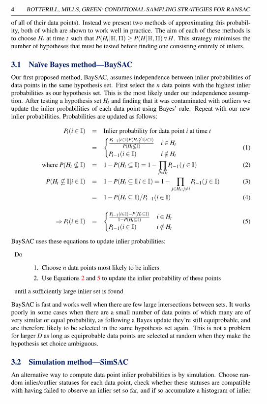
3.1 Naïve Bayes method—BaySACOur first proposed method, BaySAC, assumes independence between inlier probabilities ofdata points in the same hypothesis set. First select the n data points with the highest inlierprobabilities as our hypothesis set. This is the most likely under our independence assump-tion. After testing a hypothesis set Ht and finding that it was contaminated with outliers weupdate the inlier probabilities of each data point using Bayes’ rule. Repeat with our newinlier probabilities. Probabilities are updated as follows:
Pt(i ∈ I) = Inlier probability for data point i at time t
=
Pt−1(i∈I)P(Ht *I|i∈I)P(Ht *I) i ∈ Ht
Pt−1(i ∈ I) i /∈ Ht
(1)
where P(Ht * I) = 1−P(Ht ⊆ I) = 1−∏j∈Ht
Pt−1( j ∈ I) (2)
P(Ht * I|i ∈ I) = 1−P(Ht ⊆ I|i ∈ I) = 1− ∏j∈Ht : j 6=i
Pt−1( j ∈ I) (3)
= 1−P(Ht ⊆ I)/Pt−1(i ∈ I) (4)
⇒ Pt(i ∈ I) =
Pt−1(i∈I)−P(Ht⊆I)
1−P(Ht⊆I) i ∈ Ht
Pt−1(i ∈ I) i /∈ Ht(5)
BaySAC uses these equations to update inlier probabilities:
Do
1. Choose n data points most likely to be inliers
2. Use Equations 2 and 5 to update the inlier probability of these points
until a sufficiently large inlier set is found
BaySAC is fast and works well when there are few large intersections between sets. It workspoorly in some cases when there are a small number of data points of which many are ofvery similar or equal probability, as following a Bayes update they’re still equiprobable, andare therefore likely to be selected in the same hypothesis set again. This is not a problemfor larger D as long as equiprobable data points are selected at random when they make thehypothesis set choice ambiguous.
3.2 Simulation method—SimSACAn alternative way to compute data point inlier probabilities is by simulation. Choose ran-dom inlier/outlier statuses for each data point, check whether these statuses are compatiblewith having failed to observe an inlier set so far, and if so accumulate a histogram of inlier

BOTTERILL, MILLS, GREEN: CONDITIONAL SAMPLING STRATEGIES FOR RANSAC 5
counts for each of the D data points. The n highest peaks in this histogram form the mostlikely inlier set. SimSAC proceeds as follows:
1. Do
- Simulate random inlier/outlier statuses x1...xN ∈ 0,1D based on prior inlierprobabilities (so that P(xi = 1) = πi).
- If ∀H ∈H∃h ∈H s.t. xh = 0 then increment a counter for each simulated inlier.
until we have found T compatible simulated sets.
2. Choose the n data-points that were most frequently inliers as our next hypothesis set.
SimSAC works by sampling from the prior distribution of inlier/outlier status vectors, thenupdating this sample conditional on observing hypothesis sets that contain outliers (indicat-ing that many possible status vectors were not correct). Finding the peaks in a histogramfrom accumulating these status vectors gives us the n data points that are individually mostlikely to be inliers, conditional on the failed hypothesis set history. Assuming independencebetween inlier probabilities for the most likely inliers at time t (a much weaker assumptionthan the Naïve Bayes assumptions in BaySAC), this algorithm will give us the actual mostlikely hypothesis set at each time, as T → ∞. To avoid this assumption we would have tochoose the inlier/outlier status vector that is most frequent conditional on being drawn fromthe prior distribution, and being compatible with the observed history. This is so complex(taking time and memory Ω(exp(D))—a large fraction of possible status vectors must besimulated many times) that it is infeasable even for the smallest problems.
While SimSAC is much slower than other approaches, and still has high complexity,for practical applications it may be considerably faster than model generation. For practicalapplications choosing T = 10 samples provides a method to choose one of the more likelyhypothesis sets. A value such as T = 1000 provides a ‘ground truth’ reference–it is unlikelyany feasible algorithm can perform substantially better than this.
3.3 N–M CorrespondencesWhen searching for correspondences between two frames it is often found that multiple (N)features in one image appear sufficiently similar to multiple (M) features in the other thatthey could be the same feature. The standard approach to this situation is to limit the imagedistance between features in the two images, and/or to reject all correspondences with mul-tiple similar-looking potential matches [4, 9, 14]. The problem with this is that in visuallypoor or self-similar environments too few good correspondences may remain for scene ge-ometry to be recovered accurately, if at all. Also limiting track lengths introduces difficultiesin registering frames during rapid camera motion or following loop closure. Figure 1 showstwo images where 2–2 and 3–3 correspondences are essential to obtain enough inliers over awide enough area to recover camera motion. As a result, visual navigation systems are rarelydemonstrated in such self-similar or visually poor environments.
A better solution to this problem is to introduce correspondences between all possiblepairs of points. This leads to N×M correspondences of which at most min(N,M) are correct.If N ≤M, and the probability of one of these points i in the first image matching any of theM points in the second is p, then the probability that correspondence (i, j) is an inlier isp/M. In general, the probability that (i, j) is an inlier is p/max(N,M). Our new sampling

6 BOTTERILL, MILLS, GREEN: CONDITIONAL SAMPLING STRATEGIES FOR RANSAC
Figure 1: Frames from a video sequences used for essential matrix estimation with insuf-ficient 1-1 correspondences for these to be used alone. Of the 6 potential correspondencesshown at most 3 are correct.
algorithms, with a simple adaption to avoid choosing incompatible correspondences (if (i, j)is an inlier, (i,k) and (l, j) are not ∀k, l) can make use of these probabilities. Note that unlikeother sampling strategies (RANSAC and Guided-MLESAC) it does not matter that manycorrespondences with low probabilities are introduced, as they will only be selected as partof hypothesis sets once sufficient evidence has been observed to indicate they are more likelyto be correct than correspondences with higher prior probabilities.
If (i, j)∈Ht and Ht is contaminated by outliers, the posterior probabilities of (i,k),(l, j)∀ k, l are slightly increased (the probability of other correspondences that are incompatiblewith (i,k),(l, j) should also be slightly reduced but this amount is negligibly small). Weadapt Equation 5 as follows to take this into account:
Pt((i,k) ∈ I|(i, j) ∈ Ht) = P((i,k) ∈ I|(i, j) ∈ I)P((i, j) ∈ I|(i, j) ∈ Ht) (6)+ P((i,k) ∈ I|(i, j) /∈ I)P((i, j) /∈ I|(i, j) ∈ Ht)
=Pt−1((i,k) ∈ I)
(1−Pt−1((i, j) ∈ I))(1−Pt((i, j) ∈ I)) (7)
because (i, j) ∈ I ⇒ (i,k) /∈ I ⇒ P((i,k) ∈ I|(i, j) ∈ I) = 0 (8)
4 ResultsWe have validated our new sampling algorithms using both simulated data and real data(for the case of essential matrix estimation). When considering N–M correspondences allalgorithms are modified to avoid selecting impossible combinations: correspondences arenot selected if a previously selected correspondence shares an endpoint.
5 Results on Simulated DataTo test our new sampling algorithms we simulate the inlier/outlier statuses of D data pointswith some prior probabilities Π. We then sample repeatedly using one of our sampling strate-gies until a set consisting entirely of inliers is found. Table 2 shows the mean number of iter-

BOTTERILL, MILLS, GREEN: CONDITIONAL SAMPLING STRATEGIES FOR RANSAC 7
10 20 30 40 50 60 70 80 90 100Number of data points (D)
0
20
40
60
80
100
120
Num
ber
of
itera
tions
Sampler Performance: Prior=N-N(0.8, 2), n=8
RANSACPROSACGuided-MLESACBaySACSimSAC (T=10)SimSAC (T=1000)
Figure 2: BaySAC and SimSAC with T = 1000 reduce the number of iterations needed tofind an all-inlier hypothesis set.
ations (and a 99% confidence bound on this mean) needed to find a hypothesis set containingonly inliers, for the values D (number of data points) = 50 and n (hypothesis set size) = 5.
Several prior probability distributions are used:
Constant(p) Original RANSAC—prior probabilities all equal a constant p (p = 0.5 is shownin Table 2, similar results are observed for p = 0.25 and p = 0.75).
Unif(a,b) Prior probabilities are uniformly distributed in the range (a,b). Uniform(0.25, 0.75)are shown in Table 2—the second case corresponds to feature matches being uncertaindespite a very strong feature matcher response, together with a lower bound on allowedmatch quality. Very similar results are observed for probabilities from Uniform(0, 1).
N-N(p,N) Prior probability of one data point having a match is constant (p = 0.6 for theseexperiments), but sets of K points each have K match candidates (P(match)= p/K, K∼Unif[1, ...,N]).
Additionally, as prior probabilities are hard to estimate in advance [3], simulations are car-ried out where true prior probabilities are uniformly distributed about the estimated valuesfrom 0.25 below to 0.25 above (subject to staying within (0,1)). There is also a possibilitythat degenerate configurations incorrectly assumed to contain outliers will cause a samplingstrategy to fail. To simulate this inlier sets are rejected with probability 0.25. The number ofiterations needed under these assumptions are shown in column ‘Uncertain Π’ of Table 2.
Table 2 only shows results for the values D = 50 and n = 5. Results are comparablefor values of D from 15 to 1000 and n from 2 to 10; Figure 2 shows the consistently strongperformance of BaySAC and SimSAC for D = 15..100 and n = 8, with prior probabilitiesfrom N-N(0.8,2). Note the periodicity in the BaySAC performance–when n divides D (orthey have a high common factor) sets of n equiprobable data points remain equiprobable(and hence are selected again at the same time) following a Bayes update. Run times aregiven–these are only directly comparable for a particular number of iterations (before eithersucceeding or terminating) as different sampling strategies have different complexity, as dis-cussed in Section 5.2. In these simulations RANSAC is terminated after 250 iterations if no

8 BOTTERILL, MILLS, GREEN: CONDITIONAL SAMPLING STRATEGIES FOR RANSAC
inlier set is found (termination is essential for real-time applications), and the success rate isrecorded.
The results presented include the mean number of samples drawn when a hypothesisset is found, a 99% confidence bound on this mean and the proportion of samples whereno inlier set was found. SimSAC with T = 1000 outperforms all other methods, but is
Sampling algorithm Prior Mean iters. Success Time Mean iters.probabilities (99% bound) (%) (×10−6s) Uncertain Π
RANSAC Constant(0.5) 43.28±0.16 96 0.34 51.77±0.18PROSAC Constant(0.5) 66.85±0.29 53.2 0.447 70.1±0.3Guided-MLESAC Constant(0.5) 43.14±0.16 95.9 0.661 51.57±0.18BaySAC Constant(0.5) 41.74±0.16 96.2 1.04 50.41±0.18SimSAC (T = 10) Constant(0.5) 42.76±0.16 96 7.26 50.82±0.18SimSAC (T = 1000) Constant(0.5) 41.71±1.1 96.2 579 47.93±3.9RANSAC Unif(0.25, 0.75) 43.34±0.16 96 0.341 51.8±0.18PROSAC Unif(0.25, 0.75) 30.96±0.16 90.9 0.625 34.21±0.17Guided-MLESAC Unif(0.25, 0.75) 32.39±0.13 98.2 0.687 40.03±0.15BaySAC Unif(0.25, 0.75) 18.99±0.12 96.4 1.42 23.37±0.14SimSAC (T = 10) Unif(0.25, 0.75) 21.51±0.12 98.2 6.47 27.86±0.14SimSAC (T = 1000) Unif(0.25, 0.75) 16.47±0.68 99 479 19.9±2.3RANSAC N-N(0.6, 3) 109.1±0.43 29.5 0.386 112.7±0.48PROSAC N-N(0.6, 3) 48.61±0.29 40.6 0.687 51.86±0.31Guided-MLESAC N-N(0.6, 3) 96.32±0.35 44.5 1.07 101.2±0.38BaySAC N-N(0.6, 3) 58.8±0.38 40.9 3.59 57.61±0.38SimSAC (T = 10) N-N(0.6, 3) 61.7±0.29 56.3 10.1 65.82±0.31SimSAC (T = 1000) N-N(0.6, 3) 19.65±1.4 31.9 509 28.79±6.1
Table 2: Results on simulated data with D = 50 and n = 5.
far more costly. BaySAC performs almost as well, and considerably better that Guided-MLESAC sampling, RANSAC sampling or PROSAC sampling in most cases. Inaccurateprior probability estimates have surprisingly little effect on results. Improvements from ournew algorithms are marginal in the original case with uniform prior probabilities (althoughare more significant when D is small, e.g. D = 20), but large improvements are gained whenprior probabilities can be estimated.
The case when BaySAC does not performs quite as well is with N-N correspondences.This is the one case where there is significant room for improvement—no other algorithmcomes close to matching the 20 iterations needed by the simulated sampler with T = 1000.
Note that PROSAC sampling often performs poorly, particularly with constant priorprobabilities where it performs considerably worse than random sampling. This is because itrepeatedly samples from the same small set of data points, and when these are contaminatedwith outliers many iterations are wasted trying small variations on contaminated hypothesissets. PROSAC does not take into account the information provided by previous failures.
5.1 Results on Real DataIn order to evaluate our new RANSAC variations on real data we use them to find the es-sential matrices from the N–M correspondences (N,M ≤ 3) between consecutive pairs offrames from a 20 frame indoor and a 204 frame outdoor video sequence (Figure 3). Theprior probability model described earlier is used, with p = 0.5. Each video was processed

BOTTERILL, MILLS, GREEN: CONDITIONAL SAMPLING STRATEGIES FOR RANSAC 9
Figure 3: Frames from the indoor and outdoor sequences used for essential matrix estimation
Sampling Outdoors Indoorsalgorithm Success rate (s.d.) Inliers Success rate (s.d.) InliersRANSAC 144.0/203 (1.0) 151 16.7/19 (0.5) 131PROSAC 179.3/203 (5.0) 130 17.0/19 (0.0) 130Guided-MLESAC 186.3/203 (3.4) 129 16.3/19 (2.6) 124BaySAC 189.0/203 (0.0) 130 18.3/19 (1.1) 129SimSAC (10) 185.0/203 (2.0) 130 17.7/19 (1.1) 122SimSAC (1000) 191.3/203 (1.9) 131 18.7/19 (0.5) 131
Table 3: Essential matrix estimation—N–M correspondences from pairs of consecutiveframes from indoor and outdoor video sequences
three times, and the mean number of times a good essential matrix was found (one with atleast 15 inliers, and within a threshhold of the known camera motion) is given. The numberof iterations is limited to 250, and in practice we rarely terminate much earlier than this (asinlier rates are not high enough). As a result, run times are almost identical (0.04s per framepair). Table 3 shows that BaySAC finds the essential matrix more often than other methods,other than SimSAC with T = 1000; this takes 0.3s per frame pair so is too slow for real-time use. Note that ignoring prior probabilities entirely (original RANSAC) results in poorperformance.
We find around 400 potential correspondences per frame with N,M ≤ 3. Using only 1-1correspondences results in around 50-150 correspondences, and regularly less than 25 inliersare found from these (an average of 49 are found in the indoor sequence). We have foundthis level too low to recover an accurate camera motion estimate from these videos.
5.2 Run-times and complexityExecution times in this paper refer to C/C++ code compiled with gcc and running on onecore of a 3Ghz Intel Core 2 Duo processor.
Drawing a hypothesis set of size n using BaySAC has O(n log(D)) complexity (maintaina sorted list of D probabilities, update around n at each iteration, and select the top n). Thereis an initial setup cost of O(D log(D)).
Simulating inlier/outlier statuses for D data points takes time of O(D). Testing com-patibility with a history of size t takes time of O(tn). If prior probabilities truly reflect theinlier/outlier probabilities then few status sets need to be generated to find one compatible

10 BOTTERILL, MILLS, GREEN: CONDITIONAL SAMPLING STRATEGIES FOR RANSAC
with having not found an all-inlier set so far. This would give SimSAC a total complexity ofO(Dtn). However overly optimistic inlier probabilities lead to large numbers of status setsbeing rejected, greatly increasing this complexity.
The RANSAC application we are particularly interested in is real-time essential matrixestimation for visual odometry. Stewénius et al. [12] developed an algorithm to computethe 2-10 essential matrices compatible with five points; our C++ implementation (using theEigen matrix library [6]) takes an average of 1.4×10⁻⁴s to estimate an average of 5 matricescompatible with a hypothesis set. Validating a model for one data point takes 2.5× 10⁻⁸s,and typically few data points need to be compared in practice [2, 8], making this a smallcomponent of the total cost. For this application BaySAC’s increased sampling costs areinsignificant compared to the cost of model generation and testing (taking about 1.5×10⁻⁶sper sample with D = 50, n = 5—about 1% as long).
For applications where model generation and verification is more expensive (for exampletrifocal tensor estimation [7]) minimising the number of iterations required by using SimSACmay be worthwhile, however the improvement in the case of essential matrix estimation isnot great enough to justify the increased cost of generating samples.
6 Conclusions
BaySAC is an effective way to speed up RANSAC sampling when prior probabilities canbe estimated. In some cases the number of iterations required can be halved compared withsimple RANSAC sampling, and it significantly outperforms other sampling algorithms thatare based on estimated prior probabilities. Performance is good even when prior probabilityestimates are only approximate.
In the case of essential matrix estimation BaySAC and SimSAC can make effective use ofN−M correspondences between sets of multiple points. This allows improved performancein visually poor and self-similar environments, decreasing the probability of failing to findan essential matrix connecting two cameras by 78% in one example. BaySAC and SimSACcan also reduce the number of iterations needed when data points are assumed equally likelyto be inliers, as in the original RANSAC algorithm, although the speed-up is marginal unlessmodel generation is particularly expensive.
References[1] Matthew Brown and David G. Lowe. Automatic panoramic image stitching using in-
variant features. Int J Comput Vision, 74(1):59–73, 2007.
[2] D.P. Capel. An effective bail-out test for RANSAC consensus scoring. In Proc BritishMachine Vision Conference, pages 1–10, 2005.
[3] O. Chum and J. Matas. Matching with PROSAC - progressive sample consensus. InProc IEEE Comput Soc Conf Comput Vis Pattern Recognit, pages 220–226, Los Alami-tos, USA, 2005. ISBN 0-7695-2372-2.
[4] A.J. Davison. Real-time simultaneous localisation and mapping with a single camera.In Proc IEEE Int Conf Comput Vis, October 2003.

BOTTERILL, MILLS, GREEN: CONDITIONAL SAMPLING STRATEGIES FOR RANSAC 11
[5] Martin A. Fischler and Robert C. Bolles. Random sample consensus: a paradigm formodel fitting with applications to image analysis and automated cartography. CommunACM, 24(6):381–395, 1981. ISSN 0001-0782.
[6] Gaël Guennebaud and Benoît Jacob. Eigen 2 matrix library. URL http://eigen.tuxfamily.org/.
[7] Richard Hartley and Andrew Zisserman. Multiple View Geometry in Computer Vision.Cambridge University Press, Cambridge, UK, second edition, 2003.
[8] Jirí Matas and Ondrej Chum. Randomized RANSAC with sequential probability ratiotest. In Proc IEEE Int Conf Comput Vis, pages 1727–1732, New York, USA, October2005.
[9] D. Nistér, O. Naroditsky, and J. Bergen. Visual odometry for ground vehicle applica-tions. Journal of Field Robotics, 23(1):3–20, 2006.
[10] P. J. Rousseeuw and A. M. Leroy. Robust regression and outlier detection. John Wiley& Sons, Inc., New York, NY, USA, 1987. ISBN 0-471-85233-3.
[11] Ruwen Schnabel, Roland Wahl, and Reinhard Klein. Efficient RANSAC for point-cloud shape detection. Computer Graphics Forum, 26(2):214–226, June 2007.
[12] H. Stewénius, C. Engels, and D. Nistér. Recent developments on direct relative ori-entation. ISPRS Journal of Photogrammetry and Remote Sensing, 60:284–294, June2006.
[13] Ben J. Tordoff and David W. Murray. Guided-MLESAC: Faster image transform esti-mation by using matching priors. IEEE Trans Pattern Anal Mach Intell, 27(10):1523–1535, 2005. ISSN 0162-8828.
[14] P. H. S. Torr and D. W. Murray. The development and comparison of robust methodsfor estimating the fundamental matrix. Int J Comput Vision, 24(3):271–300, 1997.
[15] P. H. S. Torr and A. Zisserman. MLESAC: a new robust estimator with application toestimating image geometry. Comput. Vis. Image Underst., 78(1):138–156, 2000. ISSN1077-3142.