New Approaches forClustering High Dimensional Data

Jinze Liu

A dissertation submitted to the faculty of the University of North Carolina at ChapelHill in partial fulfillment of the requirements for the degree of Doctor of Philosophy inthe Department of Computer Science.

Chapel Hill2006

Approved by:

Wei Wang

Jan Prins

Leonard McMillan

Andrew Nobel

David Threadgill

c© 2006

Jinze Liu

ALL RIGHTS RESERVED

ii

ABSTRACT

JINZE LIU: New Approaches forClustering High Dimensional Data.(Under the direction of Wei Wang.)

Clustering is one of the most effective methods for analyzing datasets that contain a

large number of objects with numerous attributes. Clustering seeks to identify groups,

or clusters, of similar objects. In low dimensional space, the similarity between objects

is often evaluated by summing the difference across all of their attributes. High dimen-

sional data, however, may contain irrelevant attributes which mask the existence of

clusters. The discovery of groups of objects that are highly similar within some subsets

of relevant attributes becomes an important but challenging task. My thesis focuses

on various models and algorithms for this task.

We first present a flexible clustering model, namely OP-Cluster (Order Preserving

Cluster). Under this model, two objects are similar on a subset of attributes if the

values of these two objects induce the same relative ordering of these attributes. OP-

Clustering algorithm has demonstrated to be useful to identify co-regulated genes in

gene expression data. We also propose a semi-supervised approach to discover biolog-

ically meaningful OP-Clusters by incorporating existing gene function classifications

into the clustering process. This semi-supervised algorithm yields only OP-clusters

that are significantly enriched by genes from specific functional categories.

Real datasets are often noisy. We propose a noise-tolerant clustering algorithm for

mining frequently occuring itemsets. This algorithm is called approximate frequent

itemsets (AFI). Both the theoretical and experimental results demonstrate that our

AFI mining algorithm has higher recoverability of real clusters than any other existing

itemset mining approaches.

Pair-wise dissimilarities are often derived from original data to reduce the com-

plexities of high dimensional data. Traditional clustering algorithms taking pair-wise

dissimilarities as input often generate disjoint clusters from pair-wise dissimilarities. It

is well known that the classification model represented by disjoint clusters is inconsis-

tent with many real classifications, such gene function classifications. We develop a

iii

Poclustering algorithm, which generates overlapping clusters from pair-wise dissimilar-

ities. We prove that by allowing overlapping clusters, Poclustering fully preserves the

information of any dissimilarity matrices while traditional partitioning algorithms may

cause significant information loss.

iv

ACKNOWLEDGMENTS

My thank first goes to my advisor Wei Wang. Without her guidance, support and

encouragement, this work could not have been done. I owe my deep appreciation to

Professor Jan Prins, who has always been patient, supportive and insightful. I have

also enjoyed the inspiring discussions with Professor Leonard Mcmillan who constantly

encourage me to explore new problems.

I would also appreciate the valuable suggestions from the rest of my PhD committee:

Professors David Threadgill and Andrew Nobel. Their comments greatly improve this

thesis.

A special thank goes to other faculty members of the department of Computer

Science: Professors Ming Lin and David Stotts. I thank them for their kind assistances

and support at different stages of my study. My thank also goes to Dr. Susan Paulsen,

for her helpful suggestions in research and unconditional sharing of her experiences in

life.

I would like to acknowledge my fellow students for their continuous encouragement

and friendship. They make my graduate study more fun.

Finally, I would like to thank my grandparents, my parents, my husband Qiong

Han, and my son Erik Y. Han for their unconditional love and support.

v

TABLE OF CONTENTS

LIST OF FIGURES xii

LIST OF TABLES xviii

1 Introduction 1

1.1 High Dimensional Data . . . . . . . . . . . . . . . . . . . . . . . . . . . 2

1.2 The Challenge . . . . . . . . . . . . . . . . . . . . . . . . . . . . . . . . 5

1.2.1 The curse of dimensionality . . . . . . . . . . . . . . . . . . . . 5

1.2.2 Dissimilarity Measures . . . . . . . . . . . . . . . . . . . . . . . 5

1.2.3 Multi-Clusters Membership . . . . . . . . . . . . . . . . . . . . 7

1.2.4 Noise Tolerance . . . . . . . . . . . . . . . . . . . . . . . . . . . 7

1.2.5 Applicability to Biological Applications . . . . . . . . . . . . . . 8

1.3 State Of the Art . . . . . . . . . . . . . . . . . . . . . . . . . . . . . . 8

1.3.1 Dimensionality Reduction . . . . . . . . . . . . . . . . . . . . . 9

1.3.2 Subspace Clustering . . . . . . . . . . . . . . . . . . . . . . . . 9

1.4 Thesis statement and contributions . . . . . . . . . . . . . . . . . . . . 11

2 Background 13

2.1 Terms and Notations . . . . . . . . . . . . . . . . . . . . . . . . . . . . 13

vi

2.2 Overview of Clustering . . . . . . . . . . . . . . . . . . . . . . . . . . . 14

2.2.1 Hierarchical Clustering . . . . . . . . . . . . . . . . . . . . . . . 14

2.2.2 Clustering by Partitioning . . . . . . . . . . . . . . . . . . . . . 15

2.3 Overview of Dimensionality Reduction . . . . . . . . . . . . . . . . . . 16

2.4 Overview of Subspace Clustering . . . . . . . . . . . . . . . . . . . . . 17

2.4.1 Grid-based Subspace Clustering . . . . . . . . . . . . . . . . . . 17

2.4.2 Projection-based Subspace Clustering . . . . . . . . . . . . . . . 19

2.4.3 Bipartitioning-based Subspace Clustering . . . . . . . . . . . . . 19

2.4.4 Pattern-based Subspace Clustering . . . . . . . . . . . . . . . . 20

3 Order Preserving Subspace Clustering 22

3.1 Introduction . . . . . . . . . . . . . . . . . . . . . . . . . . . . . . . . . 22

3.2 Related Work . . . . . . . . . . . . . . . . . . . . . . . . . . . . . . . . 25

3.2.1 Subspace Clustering . . . . . . . . . . . . . . . . . . . . . . . . 25

3.2.2 Sequential Pattern Mining . . . . . . . . . . . . . . . . . . . . . 27

3.3 Model . . . . . . . . . . . . . . . . . . . . . . . . . . . . . . . . . . . . 28

3.3.1 Definitions and Problem Statement . . . . . . . . . . . . . . . . 28

3.4 Algorithm . . . . . . . . . . . . . . . . . . . . . . . . . . . . . . . . . . 31

3.4.1 Preprocessing . . . . . . . . . . . . . . . . . . . . . . . . . . . . 31

3.4.2 OPC-Tree . . . . . . . . . . . . . . . . . . . . . . . . . . . . . . 32

3.4.3 Improvement with Collapsing Node . . . . . . . . . . . . . . . . 39

3.4.4 Addition Feature: δ-pCluster . . . . . . . . . . . . . . . . . . . 39

3.4.5 Additional Feature: Extension of Grouping Technique . . . . . . 40

vii

3.5 Experiments . . . . . . . . . . . . . . . . . . . . . . . . . . . . . . . . . 40

3.5.1 Data Sets . . . . . . . . . . . . . . . . . . . . . . . . . . . . . . 40

3.5.2 Model Sensitivity Analysis . . . . . . . . . . . . . . . . . . . . . 41

3.5.3 Scalability . . . . . . . . . . . . . . . . . . . . . . . . . . . . . . 42

3.5.4 Results from Real Data . . . . . . . . . . . . . . . . . . . . . . . 43

3.6 Conclusions . . . . . . . . . . . . . . . . . . . . . . . . . . . . . . . . . 44

4 Ontology Driven Subspace Clustering 46

4.1 Introduction . . . . . . . . . . . . . . . . . . . . . . . . . . . . . . . . . 46

4.2 Ontology Framework . . . . . . . . . . . . . . . . . . . . . . . . . . . . 50

4.3 TP-Cluster Model and Ontology Interpretation . . . . . . . . . . . . . 52

4.3.1 The HTP-clustering tree . . . . . . . . . . . . . . . . . . . . . . 54

4.3.2 Annotation of a Cluster . . . . . . . . . . . . . . . . . . . . . . 54

4.3.3 Mapping the HTP-clustering tree onto Ontology . . . . . . . . . 57

4.4 Construction of Ontology Relevant HTP-clustering tree . . . . . . . . . 58

4.4.1 Construction of HTP-clustering tree . . . . . . . . . . . . . . . . 58

4.4.2 Ontology Based Pruning Techniques . . . . . . . . . . . . . . . 61

4.5 Evaluation . . . . . . . . . . . . . . . . . . . . . . . . . . . . . . . . . . 63

4.5.1 Performance Evaluation . . . . . . . . . . . . . . . . . . . . . . 64

4.5.2 Mapping between GO and the HTP-clustering tree . . . . . . . 67

4.6 Conclusions and Future Work . . . . . . . . . . . . . . . . . . . . . . . 67

5 Noise-Tolerant Subspace Clustering 70

5.1 Introduction . . . . . . . . . . . . . . . . . . . . . . . . . . . . . . . . . 71

viii

5.1.1 Fragmentation of Patterns by Noise . . . . . . . . . . . . . . . . 72

5.1.2 Approximate Frequent Itemset Models . . . . . . . . . . . . . . 74

5.1.3 Challenges and Contributions . . . . . . . . . . . . . . . . . . . 76

5.1.4 Outline . . . . . . . . . . . . . . . . . . . . . . . . . . . . . . . 78

5.2 Background and Related Work . . . . . . . . . . . . . . . . . . . . . . . 78

5.3 Recovery of Block Structures in Noise . . . . . . . . . . . . . . . . . . . 79

5.4 AFI Mining Algorithm . . . . . . . . . . . . . . . . . . . . . . . . . . . 81

5.4.1 Mining AFIs . . . . . . . . . . . . . . . . . . . . . . . . . . . . . 82

5.4.2 An Example . . . . . . . . . . . . . . . . . . . . . . . . . . . . . 85

5.4.3 Global Pruning . . . . . . . . . . . . . . . . . . . . . . . . . . . 86

5.4.4 Identification of AFI . . . . . . . . . . . . . . . . . . . . . . . . 87

5.5 Experiments . . . . . . . . . . . . . . . . . . . . . . . . . . . . . . . . . 88

5.5.1 Scalability . . . . . . . . . . . . . . . . . . . . . . . . . . . . . . 88

5.5.2 Quality Testing with Synthetic Data . . . . . . . . . . . . . . . 90

5.5.3 Zoo Data Set . . . . . . . . . . . . . . . . . . . . . . . . . . . . 91

5.6 Conclusion . . . . . . . . . . . . . . . . . . . . . . . . . . . . . . . . . . 93

5.7 Appendix . . . . . . . . . . . . . . . . . . . . . . . . . . . . . . . . . . 93

6 Clustering Dissimilarity Data into Partially Ordered Set 96

6.1 Introduction . . . . . . . . . . . . . . . . . . . . . . . . . . . . . . . . . 96

6.2 Related Work . . . . . . . . . . . . . . . . . . . . . . . . . . . . . . . . 100

6.2.1 Hierarchial and Pyramidal Clustering . . . . . . . . . . . . . . . 100

6.2.2 Dissimilarity Derived from Ontology Structure . . . . . . . . . . 101

ix

6.3 Preliminaries . . . . . . . . . . . . . . . . . . . . . . . . . . . . . . . . 102

6.4 Model . . . . . . . . . . . . . . . . . . . . . . . . . . . . . . . . . . . . 102

6.4.1 Relationships with Hierarchy and Pyramid . . . . . . . . . . . . 105

6.5 PoCluster Derivable Ontology . . . . . . . . . . . . . . . . . . . . . . . 106

6.5.1 The Implication of PoCluster on Dissimilarities . . . . . . . . . 108

6.5.2 Algorithm of Deriving Dissimilarities . . . . . . . . . . . . . . . 110

6.6 PoClustering Algorithm . . . . . . . . . . . . . . . . . . . . . . . . . . 112

6.7 Experiments . . . . . . . . . . . . . . . . . . . . . . . . . . . . . . . . . 114

6.7.1 Evaluation Criteria . . . . . . . . . . . . . . . . . . . . . . . . . 114

6.7.2 Synthetic Data . . . . . . . . . . . . . . . . . . . . . . . . . . . 114

6.7.3 Gene Ontology . . . . . . . . . . . . . . . . . . . . . . . . . . . 116

6.8 Conclusions . . . . . . . . . . . . . . . . . . . . . . . . . . . . . . . . . 117

7 Visualization Framework to Summarize and Explore Clusters 122

7.1 Introduction . . . . . . . . . . . . . . . . . . . . . . . . . . . . . . . . . 122

7.2 Related Work . . . . . . . . . . . . . . . . . . . . . . . . . . . . . . . . 124

7.2.1 Cluster and Subspace Cluster Visualization . . . . . . . . . . . . 124

7.2.2 Postprocessing of Subspace Clusters . . . . . . . . . . . . . . . . 125

7.3 Model . . . . . . . . . . . . . . . . . . . . . . . . . . . . . . . . . . . . 125

7.3.1 Subspace Cluster . . . . . . . . . . . . . . . . . . . . . . . . . . 125

7.3.2 Coverage Dissimilarity . . . . . . . . . . . . . . . . . . . . . . . 126

7.3.3 Pattern Dissimilarity . . . . . . . . . . . . . . . . . . . . . . . . 127

7.3.4 Blending of Dissimilarities . . . . . . . . . . . . . . . . . . . . . 128

x

7.3.5 View of A Set of Subspace Clusters . . . . . . . . . . . . . . . . 129

7.4 Methods . . . . . . . . . . . . . . . . . . . . . . . . . . . . . . . . . . . 130

7.4.1 MDS and fastMDS . . . . . . . . . . . . . . . . . . . . . . . . . 130

7.4.2 fastMDS . . . . . . . . . . . . . . . . . . . . . . . . . . . . . . . 131

7.4.3 Visualization of Clustering . . . . . . . . . . . . . . . . . . . . . 132

7.5 Experiments . . . . . . . . . . . . . . . . . . . . . . . . . . . . . . . . . 133

7.5.1 Results on Zoo Dataset. . . . . . . . . . . . . . . . . . . . . . . 133

7.5.2 Results on Gene Expression Dataset . . . . . . . . . . . . . . . 134

7.6 Conclusion . . . . . . . . . . . . . . . . . . . . . . . . . . . . . . . . . . 135

8 Conclusion and Future Work 138

Bibliography 141

xi

LIST OF FIGURES

1.1 An example of gene expression data matrix with 3447

genes and 18 conditions. The expression levels are mapped

to a heatmap, where red corresponds to high expression

level and blue corresponds to low expression level . . . . . . . . . . . . 2

1.2 An example of transactional database and its binary for-

mat . . . . . . . . . . . . . . . . . . . . . . . . . . . . . . . . . . . . . 3

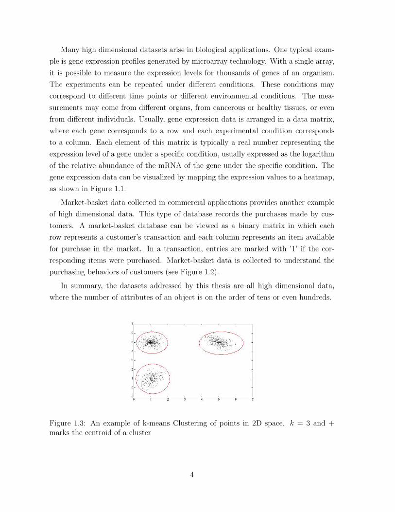
1.3 An example of k-means Clustering of points in 2D space.

k = 3 and + marks the centroid of a cluster . . . . . . . . . . . . . . . 4

1.4 As the dimensionality goes higher,points in the space are

more spread out. . . . . . . . . . . . . . . . . . . . . . . . . . . . . . . 6

3.1 An Example of OP-cluster . . . . . . . . . . . . . . . . . . . . . . . . . 23

3.2 Comparison of clusters discovered by OPSM and OP-Clustering . . . . 27

3.3 OPC-Tree for Table 4.2. The label in the oval shape

represents the column. The number following ’:’ repre-

sents the row ID. The node with double oval means active

node in the depth first traveral. ’ !No’ means the must-be-

pruned subtree. ’Yes’ means a valid subtree. A) . Initiate

the tree with all the rows B). Insert the suffix of -1’s sub-

trees to -1’s subtrees. C). Prune the subtree (nr < 3),

Insertion. D). Identify the first E). Finish growing the

-1’s first subtree-1a, the next is -1d. . . . . . . . . . . . . . . . . . . . 34

3.4 Collapsing OPC-Tree for Table 4.2. Sequences in the

large vertical oval means collapsed nodes . . . . . . . . . . . . . . . . . 38

3.5 Performance Study: cluster number and cluster size V.S.similarity

threshold . . . . . . . . . . . . . . . . . . . . . . . . . . . . . . . . . . . 41

3.6 Performance Study: Response time V.S. number of columns

and number of rows . . . . . . . . . . . . . . . . . . . . . . . . . . . . . 42

xii

3.7 Performance comparison of prefixSpan and UPC-tree . . . . . . . . . . 43

3.8 Performance Study: Response time V.S. similarity thresh-

old , nc and nr . . . . . . . . . . . . . . . . . . . . . . . . . . . . . . . 44

3.9 Cluster Analysis: Two examples OPC-Tree in yeast data . . . . . . . . 44

3.10 Cluster Analysis: Two examples OPC-Tree in drug ac-

tivity data . . . . . . . . . . . . . . . . . . . . . . . . . . . . . . . . . . 45

4.1 An animal ontology and subspace clusters corresponding

to each category . . . . . . . . . . . . . . . . . . . . . . . . . . . . . . . 48

4.2 Schema of GO annotation terms. . . . . . . . . . . . . . . . . . . . . . 51

4.3 The maximal hierarchy of the TP-Clusters given a con-

dition space A={a, b, c}. . . . . . . . . . . . . . . . . . . . . . . . . . . 55

4.4 An example of OST representing a Cluster. The two

values in each node represent the function category and

its P-value. . . . . . . . . . . . . . . . . . . . . . . . . . . . . . . . . . 56

4.5 An example of two OST s H1 and H2, H2 ≺ H1. . . . . . . . . . . . . . 57

4.6 The illustration of suffix tree concatenation. . . . . . . . . . . . . . . . 59

4.7 The performance of the ODTP-clustering varying nr and

θp. . . . . . . . . . . . . . . . . . . . . . . . . . . . . . . . . . . . . . . 64

4.8 The comparison between ODTP-clustering and HTP-clustering. . . . . 65

4.9 The comparison of performance of ODTP-clustering among

three categories. . . . . . . . . . . . . . . . . . . . . . . . . . . . . . . 65

4.10 An example of mapping from a hierarchy of TP-Clusters

to their OST s. For each cluster in (A), the rows corre-

spond to conditions while the columns correspond to the

genes. . . . . . . . . . . . . . . . . . . . . . . . . . . . . . . . . . . . . 69

5.1 Patterns with and without noise. . . . . . . . . . . . . . . . . . . . . . . . 71

xiii

5.2 When noise is present, the observed size of the largest square

sub-matrix of 1’s increases far more slowly than the size of

the initial square matrix of 1’s. (Note: noise ratio refers to

the value of p). . . . . . . . . . . . . . . . . . . . . . . . . . . . . . . . . 73

5.3 A binary matrix with three weak AFI(0.25) They can be more

specifically classified as, A: AFI(0.25, 0.25); B: AFI(*, 0.25);

C: AFI(0.25, *). . . . . . . . . . . . . . . . . . . . . . . . . . . . . . . . 75

5.4 Relationships of various AFI criteria. . . . . . . . . . . . . . . . . . . . . 77

5.5 (A) Sample database; (B) Level wise mining of AFI in database

(A). See Section 5.4.2 for more details. Only black colored

itemsets will be generated by AFI, while every itemset in-

cluding the grey-colored itemsets will have to be generated

to mine ETIs. . . . . . . . . . . . . . . . . . . . . . . . . . . . . . . . . 85

5.6 Comparison between AFI and ETI . . . . . . . . . . . . . . . . . . . . . . 88

5.7 The running time of AFI with noise-tolerant support pruning

varying minsup and ε. ε = εc = εr. . . . . . . . . . . . . . . . . . . . . . 89

5.8 The running time of AFI with noise-tolerant support pruning

as minsup varies. εc 6= εr. . . . . . . . . . . . . . . . . . . . . . . . . . . 89

5.9 Algorithm quality versus noise level. . . . . . . . . . . . . . . . . . . . . . 91

5.10 Three AFI blocks discovered in the zoo dataset. * indicates

the presence of a feature. . . . . . . . . . . . . . . . . . . . . . . . . . . 92

xiv

6.1 (a.1) An ultrametric dissimilarity matrix; (a.2) Hierarchy

constructed from (a.1) by either hierarchical clustering or

PoClustering; (b.1) A non-metric dissimilarity matrix. (b.2)

PoCluster constructed from (b.1) by PoClustering. Note:

(a.1) can be derived from the hierarchy in (a.2) by assign-

ing each pair the minimum diameter of the sets containing

it; (b.2) can be used to derive dissimilarities of (b.1) in the

same way; Applying hierarchical clustering to (b.1) can also

construct the hierarchy in (a.2), but (b.1) cannot be derived

from (a.2) . . . . . . . . . . . . . . . . . . . . . . . . . . . . . . . . . . 98

6.2 A running example. (a) shows a dissimilarity matrix of 5

objects {A, B, C, D, E}; (b) shows an undirected weighted

graph implied by (c); Table (c) contains the list of clique clus-

ters with all diameters; (d) shows a PoCluster which contains

13 clusters and their subset relationships (Each cluster in the

PoCluster represents a clique cluster with its diameter in (c).

The PoCluster is organized in DAG with subset relationship

between the nodes. There is a directed path from node S1

to S2 if S1 ⊂ S2). Note: Applying PoClustering algorithm

can construct PoCluster shown in (d) given dissimilarity ma-

trix (a). Applying Algorithm in Section 6.5.2 can derive the

dissimilarities in (a) from PoCluster in (d). . . . . . . . . . . . . . . . . . 119

6.3 Four directed weighted graphs corresponding to the dissim-

ilarity matrix in Figure 6.2 (B) with maximum edge weight

{d = 1, 2, 3, 4}. . . . . . . . . . . . . . . . . . . . . . . . . . . . . . . . . 120

6.4 A structure of Robinson matrix. There exists a linear order-

ing of the objects, such that the dissimilarity never decreases

as they move away from diagonal along both row and column. . . . . . . . 120

6.5 An example graph with nodes {1,2,3,4,5,6,7}. All the cliques

in the graph are {1234, 1256, 2467, 1246, 2567}; The Mini-

mum ECC is {1234, 1256, 2467, 2567}. . . . . . . . . . . . . . . . . . . . 120

6.6 Experimentation on synthetic data . . . . . . . . . . . . . . . . . . . . . . 121

xv

7.1 Left: A visualization of the overlap between the yellow

and blue sets of subspace clusters as shown in the image

on the right. The intersection of the two sets of subspace

clusters is shown in green. There are over 10 subspace

clusters in each set. Right: The 3D point-cloud view of

subspace clusters. . . . . . . . . . . . . . . . . . . . . . . . . . . . . . 123

7.2 The relationships between two overlapping clusters. The

green and blue rectangles represent two separate sub-

space clusters. The yellow region is the intersection of

two. The whole region including green, blue, yellow and

white is the merged (or unioned) cluster of the two clusters. . . . . . . 126

7.3 Example of two subspace clusters. (A) is the heatmap

of a δ−pCluster; (B) is an itemset cluster, where each *

represents a 1 entry. . . . . . . . . . . . . . . . . . . . . . . . . . . . . 127

7.4 The top row of matrices (a),(b),(c) represent pattern dis-

similarity. The bottom row (d),(e),(f) represents cover-

age dissimilarity. (a) The original pattern dissimilarity

matrix; (b) Permuted pattern dissimilarity matrix, based

on the clustering of subspace clusters by pattern dissim-

ilarity alone; (c) Permuted pattern dissimilarity matrix

based on the clustering by a 50/50 blend of both pat-

tern and coverage dissimilarity; (d) The original coverage

dissimilarity matrix; (e) Permuted coverage dissimilar-

ity matrix, based on clustering subspace clusters on just

coverage dissimilarity; (f) Permuted coverage dissimilar-

ity matrix based on a 50/50 blend of both pattern and

coverage dissimilarity; (g) Blended Matrix of both pat-

tern dissimilarity and coverage dissimilarity, permuted to

show clustering . . . . . . . . . . . . . . . . . . . . . . . . . . . . . . . 129

xvi

7.5 Results of the Zoo dataset. Middle: The 3D point-cloud

view of subspace clusters by applying MDS on the com-

bined dissimilarity of coverage and pattern dissimilarities.

Each different color represent a cluster. The red points

circled in red in each cluster refers to the subspace clus-

ter that is the representative of the cluster containing it.

The three clusters can be easily classified into Mammals,

Aquatic, and Birds. Side panels: the relationships and

summary between the representative cluster and the rest

of the cluster. The red colored rectangle corresponds to

the representative cluster, which is a large fraction of the

summary of the set of subspace clusters. . . . . . . . . . . . . . . . . . 135

7.6 Result of Gene expression. Right: The 3D point cloud

view of subspace clusters. (a) Left Panel: the relation-

ships between two distant sets of subspace clusters in

the original matrix. Their dissimilarity relationships are

shown in the point cloud view. (b) Left panel: the rela-

tionships of two similar sets of subspace clusters in the

original data matrix. The two selected clusters are shown

in the two sets of points in the point cloud view. Note:

The blue histograms on top of the data matrix are gene

expression patterns of the representative subspace cluster

in the set. . . . . . . . . . . . . . . . . . . . . . . . . . . . . . . . . . . 137

xvii

LIST OF TABLES

3.1 Example Data Set . . . . . . . . . . . . . . . . . . . . . . . . . . . . . 32

4.1 A database for a subset of zoo animals . . . . . . . . . . . . . . . . . . 48

4.2 Example Data Set. . . . . . . . . . . . . . . . . . . . . . . . . . . . . . 52

4.3 Statistics for the three categories. . . . . . . . . . . . . . . . . . . . . . 64

6.1 PoCluster generated based on dissimilarity matrix in Figure 6.2(B). . . . . . 104

6.2 Two ranking of sets in the PoCluster shown in Figure 6.2(d). . . . . . . . . 108

6.3 Statistics for the three GO files. MF: Molecular Function,

CC: Cellular Component; BP: Biological Process . . . . . . . . . . . . . . 116

6.4 Reconstructed poset match score to original GO based on

various similarity measures . . . . . . . . . . . . . . . . . . . . . . . . . . 117

6.5 Reconstructed poset match score to original GO by the three

algorithms. go represents the GO file and P is the recon-

structed poset . . . . . . . . . . . . . . . . . . . . . . . . . . . . . . . . 117

xviii

Chapter 1

Introduction

Clustering is one of the most effective methods for analyzing datasets that contain a

large number of objects with numerous attributes. Clustering seeks to identify groups,

or clusters, of similar objects. Traditionally, a cluster is defined as a subset of objects

that take similar values at each attribute. A more general notion of cluster is a subset

of objects which are more similar to each other than they are to the objects in other

clusters.

Clustering results are frequently determined by dissimilarities between pairs of ob-

jects. If the objects with d attributes are viewed as points in a d-dimensional Euclidean

space, distances can be adopted as a dissimilarity measure. A variety of alternative

dissimilarity measures have been created to capture pair-wise relationships in differ-

ent applications. These pair-wise dissimilarity measures are often a summary of the

dissimilarities across all the attributes.

Traditional clustering algorithms have been successfully applied to low-dimensional

data, such as geographical data or spatial data, where the number of attributes is

typically small. While objects in some datasets can be naturally described by 3 or

fewer attributes, researchers often collect as many attributes as possible to avoid missing

anything important. As a result, many datasets contain objects with tens of or even

hundreds of attributes. We call such objects high dimensional data.

Clustering can be naturally extended to analyze high dimensional data, which re-

sults in groups of objects that are similar to each other along all the attributes. How-

ever, unlike low dimensional data where each of the attributes is considered equally

informative, not all the attributes are typically relevant in characterizing a cluster.

Dissimilarities computed along all attributes including those irrelevant ones can be ar-

bitrarily high, which, in turn, prohibits the true clusters from being discovered. Hence,

the discovery of groups of objects that are highly similar within some relevant subset

of attributes (thus eliminating irrelevant attributes) becomes an important but chal-

lenging task. My thesis focuses on various models and algorithms for this task.

In this chapter, we first describe high dimensional data and depict the challenges

encountered in the analysis of high-dimensional data. We then discuss the state of the

art in clustering approaches that aim to tackle these challenges. We conclude with a

discussion of the thesis contribution.

1.1 High Dimensional Data

Figure 1.1: An example of gene expression data matrix with 3447 genes and 18 condi-tions. The expression levels are mapped to a heatmap, where red corresponds to highexpression level and blue corresponds to low expression level

Recent technology advances have made data collection easy and fast, resulting in

large datasets that record values of hundreds of attributes for millions of objects.

2

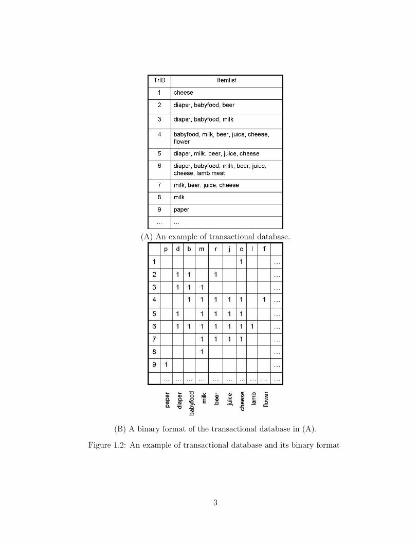
(A) An example of transactional database.

(B) A binary format of the transactional database in (A).

Figure 1.2: An example of transactional database and its binary format

3

Many high dimensional datasets arise in biological applications. One typical exam-

ple is gene expression profiles generated by microarray technology. With a single array,

it is possible to measure the expression levels for thousands of genes of an organism.

The experiments can be repeated under different conditions. These conditions may

correspond to different time points or different environmental conditions. The mea-

surements may come from different organs, from cancerous or healthy tissues, or even

from different individuals. Usually, gene expression data is arranged in a data matrix,

where each gene corresponds to a row and each experimental condition corresponds

to a column. Each element of this matrix is typically a real number representing the

expression level of a gene under a specific condition, usually expressed as the logarithm

of the relative abundance of the mRNA of the gene under the specific condition. The

gene expression data can be visualized by mapping the expression values to a heatmap,

as shown in Figure 1.1.

Market-basket data collected in commercial applications provides another example

of high dimensional data. This type of database records the purchases made by cus-

tomers. A market-basket database can be viewed as a binary matrix in which each

row represents a customer’s transaction and each column represents an item available

for purchase in the market. In a transaction, entries are marked with ’1’ if the cor-

responding items were purchased. Market-basket data is collected to understand the

purchasing behaviors of customers (see Figure 1.2).

In summary, the datasets addressed by this thesis are all high dimensional data,

where the number of attributes of an object is on the order of tens or even hundreds.

Figure 1.3: An example of k-means Clustering of points in 2D space. k = 3 and +marks the centroid of a cluster

4

1.2 The Challenge

High-dimensional data requires greater computational power. However, a much bigger

challenge is introduced by the high dimensionality itself, where the underlying associa-

tions between objects and attributes are not always strong and noise is often prevalent.

Hence, the effectiveness of any approach to accurately identify salient clusters becomes

a real concern. The rest of this section details the challenges faced in high dimensional

data.

1.2.1 The curse of dimensionality

One immediate problem faced in high dimensional data analysis is the curse of di-

mensionality, that is, as the number of dimensions in a dataset increases, evaluating

distance across all attributes become increasingly meaningless.

When we consider each object as a point in Euclidean space, it has been observed

(Parsons et al., 2004) that the points in high dimensional space are more spread out

than in a lower dimensional space. In the very extreme case with very high dimensions,

all points are almost equidistant from each other. In this case, the traditional definition

of clusters as a set of points that are closer to each other than to the rest of points does

not easily apply. Clustering approaches become ineffective to analyze the data.

The phenomena of the curse of the dimensionality is illustrated by the following

example. A high dimensional space can be created by repeatedly adding additional di-

mensions starting from an initial low dimensional space as shown in Figure 1.4 (Parsons

et al., 2004). Initially, there exists a set of closely located points in one dimensional

space. As the set of points expands to a new space by adding additional dimension,

they are more spread out and finding a meaningful cluster gets harder.

As a result, when the set of attributes in a dataset becomes larger and more varied,

clustering of objects considering across all dimensions becomes problematic.

1.2.2 Dissimilarity Measures

When the objects are viewed as points in high dimensional space, the dissimilarity

between objects is often determined based on spatial distance functions. Well-known

distance functions include Euclidean distance, Manhattan distance, and cosine distance.

These criteria often generate clusters that tend to minimize the variance of objects in

each attribute.

5

Figure 1.4: As the dimensionality goes higher,points in the space are more spread out.

6

However, these distance functions are not always sufficient for capturing the corre-

lations among objects. In the case of gene expression analysis, it may be more useful

to identify more complex relations between the genes and the conditions regardless

of their spatial distances. For example, we may be interested in finding a subset of

genes that are either consistently increasing or consistently decreasing across a subset

of conditions without taking into account their actual expression values; or we may be

interested in identifying a subset of conditions that always have the positive or negative

effect on a subset of genes. Strong correlations may exist between two objects even if

they are far apart in distance.

1.2.3 Multi-Clusters Membership

Clustering is also referred to as an unsupervised learning of classification structure,

where each cluster corresponds to a learned classification category. Most existing clus-

tering algorithms require clusters to be flat or hierarchial partitions. Therefore, one

object is not allowed to belong to multiple clusters (at the same level).

However, high dimensional data provides much richer information regarding each

object than low dimensional data. An object might be similar to a subset of objects

under one subset of attributes but also similar to a different subset of objects under

another set of attributes. Therefore, an object may be a member of multiple clusters.

However, multi-cluster membership is prohibited by traditional clustering algorithms

which typically generate disjoint clusters.

1.2.4 Noise Tolerance

Datasets collected in real applications often include error or noise. In a transaction

database, noise can arise from both recording errors of the inventories and the vagaries

of human behavior. Items expected to be purchased together by a customer might not

appear together in a particular transaction because an item is out of stock or because

it is overstocked by the customer. Microarray data is likewise subject to measurement

noise, stemming from the underlying experimental technology and the stochastic nature

of the biological systems.

In general, the noise present in real applications undermines the ultimate goal of

traditional clustering algorithms: recovering consistent clusters amongst the set of at-

tributes considered. As a matter of fact, the presence of noise often breaks the real

underlying clusters into small fragments. Applying existing algorithms recovers these

7

fragments while missing the real underlying clusters. The problem is worsened in high

dimensional data, where the number of errors increases linearly with dimensionality.

Noise-tolerance in clustering is very important to understand the real cluster struc-

tures in the datasets. However, distinguishing noise from accurate and relevant values

is hard, consequently, searching for noise-tolerant clusters is even harder since many

large potential clusters need to be considered in order to identify the real clusters.

1.2.5 Applicability to Biological Applications

Clustering has been one of the popular approaches for gene expression analysis. The

feasibility for applying clustering to gene expression analysis is supported by the hy-

pothesis that genes participating in the same cellular process often exhibit similar

behavior in their expression profiles. Unfortunately, traditional clustering algorithms

do not suit the needs of gene expression data analysis well, due to a variety of biological

complications. First, an interesting cellular process may be active only in a subset of

the conditions. Genes co-regulated under these conditions may act independently and

show random expression profiles under other conditions. Computing dissimilarities by

evaluating all conditions, as adopted by traditional clustering approaches, may mask

the high similarity exhibited by genes under a subset of conditions, which in turn, pro-

hibits the discovery of genes that participate in the cellular process. Secondly, a gene

may have multiple functions. It may be involved in multiple biological pathways or in

no pathways at all. However, the classification model underlying most of the traditional

clustering algorithms forces one gene to be a member of exactly one cluster. This clas-

sification model itself is too restrictive to represent the more complicated classification

model underlying gene functions. A desirable clustering algorithm applicable to gene

expression analysis should have the following characteristics.

• A cluster of genes should be defined with respect to a subset of relevant conditions.

• Overlapping should be allowed between two clusters, i.e, a gene/condition is al-

lowed to belong to more than one cluster or to no cluster at all.

1.3 State Of the Art

The state of the art methods for clustering high dimensional data can be divided into

the following two categories: dimensionality reduction and subspace clustering.

8

1.3.1 Dimensionality Reduction

Dimensionality reduction techniques include both feature transformation and feature

selection. Two representative examples of feature transformation techniques include

principal component analysis (PCA) and multi-dimensional scaling (MDS). The goal

of PCA and MDS is to find the minimum set of dimensions that capture the most

variance in a dataset. More precisely, PCA is based on computing the low dimen-

sional representation of a high dimensional data set that most faithfully preserves its

covariance structure. MDS is based on computing the low dimensional representation

of a high dimensional data set that most faithfully preserves dissimilarities between

different objects. Though based on a somewhat different geometric intuitions, the two

approaches generate similar results. The dimensionality reduction techniques are not

ideal for clustering since they are not able to eliminate irrelevant attributes that mask

the clusters. In addition, the new features derived from either PCA or MDS are linear

combinations of the original features. They are not straightforward to interpret in real

applications, especially when each of them carries independent meanings.

As suggested by its name, feature selection methods attempt to select a proper sub-

set of features that best satisfies a relevant function or evaluation criterion. The results

of feature selection make it possible to reduce storage, to reduce the noise generated

by irrelevant features and to eliminate useless features. While feature selection meth-

ods find the most important features (subspaces), they may fail to discover multiple

independent subspaces, which contain significant clusters.

1.3.2 Subspace Clustering

Subspace clustering algorithms take the concept of feature selection one step further by

selecting relevant subspaces for each cluster independently. These algorithms attempt

to find the clusters and their subspaces simultaneously. Subspace clustering is also

called biclustering or co-clustering since the algorithm clusters objects and attributes

at the same time.

One branch of subspace clustering algorithm divides both the set of objects and the

set of attributes into disjoint partitions, where the partitions maximize global objective

functions(Dhillon et al., 2003; Chakrabarti et al., 2004). Even though a globally optimal

partition may be reached, the local properties of a single cluster generated by partition-

based clustering is hard to characterize. In addition, since each object belongs to exactly

one cluster and so does each attribute, partition-based subspace clustering does not fit

9

the needs of certain applications where an object and/or an attribute may belong to

multiple clusters or to no cluster at all.

The other branch of subspace clustering algorithms, eliminates the restriction of

partition-based algorithms by looking for clusters satisfying given criteria. These crite-

ria define the properties of desired clusters. These clustering algorithms are also called

pattern-based algorithms. Unlike partition-based algorithms that search for the best

global partitions, pattern-based algorithms do not restrict one object to a single clus-

ter. Instead, pattern-based algorithms guarantees that any clusters they generate must

satisfy the cluster pattern criteria.

Pattern-based algorithms can be different from each other based on the type of

patterns they are looking for. One of the natural patterns is a set of objects (points)

closely located together in high dimensional space. The algorithms to search for this

type of clusters has been extensively studied in (Agrawal et al., 1998; Cheng et al.,

1999; Nagesh et al., 1999; Aggarwal et al., 1999; Aggarwal and Yu, 2000). Subspace

clustering based on spatial distance is limited in its ability to find clusters with high

correlations. In biological applications, genes that are far apart from each other may

still exhibit consistent up and down regulations under a subset of conditions, which

are called co-regulation patterns. Recently, clustering algorithm such as residue-based

biclustering (Cheng and Church, 2000), Order preserving biclustering (Ben-Dor et al.,

2002) and the search of shifting and scaling patterns (Wang et al., 2002) were developed

to look for specific co-regulation patterns.

Not all the algorithms above generate the complete set of patterns. Some take a

greedy approach of finding one maximal pattern at a time, as in (Cheng and Church,

2000; Ben-Dor et al., 2002). These algorithms often carry a polynomial time complexity

with regard to the number of objects and the number of attributes for searching one

cluster. Such algorithms may not identify a globally optimal solution and they may

miss many important subspace clusters as well.

The exhaustive approach is adopted by a number of subspace clustering algorithms

(Wang et al., 2002; Agrawal et al., 1998; Cheng et al., 1999). Rather than identifying

one or a subset of clusters at a time, the exhaustive approach finds the complete set of

subspace clusters satisfying the pattern criteria. My thesis work follows the line of the

pattern-based exhaustive subspace clustering algorithms.

10

1.4 Thesis statement and contributions

Thesis Statement: Techniques developed in this work identify clusters in subspaces

of high dimensional data with different criteria for similarity and in the presence of

noise. The clusters found using these techniques are relevant to important application

domains. The performance of these clustering techniques scales to large datasets.

The goals of this research are studying new clustering models to analyze high dimen-

sional data, deriving algorithms based on these models and subsequently performing

detailed experiments to demonstrate the efficiency and effectiveness of these algorithms

on different domains.

Each of the clustering algorithms proposed in this thesis tackle a combination of

two or more of the independent challenges arising from high dimensional data. In order

to minimize the effect of the irrelevant features on clustering, we design algorithms that

conduct clustering and the relevant subspace selection simultaneously. We also refine

clustering criteria to incorporate similarity measurements in order to reveal hidden pat-

terns arising from biological data or noisy data. In addition, we go beyond the disjoint

clustering approach by allowing overlap between clusters, which has been demonstrated

to be necessary for real biological applications.

The contributions of this thesis are:

• We propose a flexible clustering model, namely OP-Cluster (Order Preserving

Cluster). Under this model, two objects are similar on a subset of dimensions if the

values of these two objects induce the same relative ordering of these dimensions.

Such a cluster arises when the expression levels of (coregulated) genes rise or fall

together in response to a sequence of environment stimuli. Hence, the discovery

of OP-Cluster may prove useful for revealing significant gene regulatory networks.

• We propose a semi-supervised approach to discover biologically meaningful OP-

Clusters. Our approach incorporates existing gene function classifications, such

as Gene Ontology, into the clustering process, yielding only OP-clusters that are

significantly enriched with genes from a particular functional categories.

• We propose a noise-tolerant itemset model, which we call approximate frequent

itemsets (AFI). The AFI model extends traditional exact frequent itemset model

by tolerating a controlled fraction of errors in each item and each supporting

transaction. Both the theoretical and experimental results demonstrate that the

AFI criterion is well suited to the recovery of real clusters in the presence of noise.

11

• We propose a general approach for postprocessing subspace clusters (AFIs). A di-

rect consequence of subspace clustering and itemset mining is an overwhelmingly

large set of overlapping clusters, which hinders the interpretability of clustering

results. To reveal the true underlying clusters, we propose several similarity mea-

surements for subspaces clusters and adopt multi-dimensional scaling to allow the

exploration and analysis of subspace clusters.

• We study the space of partially ordered sets that are derivable from pair-wise

dissimilarity-based clustering methods. We prove that the set of PoClusters,

generated by Poclustering of dissimilarity data, has one-to-one correspondence

with the set of all dissimilarity matrices. We present the necessary and sufficient

conditions to determine whether the information a given poset may be coded loss-

less by a dissimilarity matrix. An optimal incremental algorithm and a heuristic

clustering algorithm to derive Poclusters are developed.

12

Chapter 2

Background

This chapter focuses on the current state of the art clustering algorithms. Each section

in this chapter will cover one of the clustering approaches.

2.1 Terms and Notations

Here is the notation used in the rest of the thesis. We will be working with a n ×mmatrix D, where each element Dij is a real or binary value. The set of rows in D

corresponds to a set of objects denoted by O and the set of columns corresponds to the

set of attributes (conditions) denoted by A.

In the view of the space, A refers to the set of m-dimensional attributes, i.e.,

{a1, a2, ..., am}. They are bounded and totally ordered. S denotes the full space of

A, which is a1×a2× . . .×am, a m-dimensional numerical space. Each object i in O is

represented by m-dimensional vector where vi = < vi1, vi2, . . . , vid >. The jth compo-

nent of vi is drawn from domain aj.

In gene expression data, each object is a gene, and each attribute may represent

an experimental condition or tissue sample. An entry in the matrix Dij represents the

expression level of a gene i under condition j.

In transactional database, each row of D corresponds to a transaction i and each

column of j corresponds to an item a. The i, j-th element of D, denoted D(i, j), is 1 if

transaction o contains item a, and 0 otherwise.

Given the data matrix D, as defined above, we define a row cluster as a subset of

rows that exhibit similar behavior across the set of all columns.

This means that a row cluster C = (I, A) is a subset of rows defined over the set

of all columns A (the full space) , where I ⊆ O. Similarly, a column cluster is a subset

of columns that exhibit similar behavior across the set of all rows. A column cluster

C = (O, J) is a subset of columns (a subspace) defined over the set of all rows O, where

J ⊆ A.

A subspace cluster (bicluster) is a subset of rows that exhibit similar behavior across

a subset of columns, and vice versa. The bicluster C = (I, J) is thus a subset of rows

and a subset of columns where I ⊆ O and J ⊆ A.

We frequently refer to objects as rows and attributes as columns.

2.2 Overview of Clustering

The main objective of clustering is to find high quality clusters within a reasonable

time. However, different approaches to clustering often define clusters in different

ways. Traditionally clustering techniques are broadly divided into hierarchical and

partitioning methods. Partitioning methods can be further divided into distribution-

based, density-based and grid-based methods. In this section, we review the existing

clustering approaches following this taxonomy.

2.2.1 Hierarchical Clustering

Hierarchical clustering (Karypis et al., 1999; Guha et al., 1998; Guha et al., 2000)

builds a cluster hierarchy or, in other words, a tree of clusters, often represented in a

dendrogram. Such an approach allows exploring data on different levels of granular-

ity. Hierarchical clustering can be further categorized into agglomerative and divisive

methods based on how it is constructed. An agglomerative clustering starts with one-

point (singleton) clusters and recursively merges two or more of the most appropriate

clusters. A divisive clustering starts with one cluster of all data points and recursively

splits the most appropriate cluster. The process continues until a stopping criterion is

achieved. In hierarchical clustering, the regular object-by-attribute data representation

is sometimes of secondary importance. Instead, hierarchical clustering deals with the

N × N dissimilarities between each pair of objects. Therefore, hierarchical clustering

provides the ease of handling many forms of dissimilarity or distance measures.

Hierarchical clustering proceeds iteratively with merging or splitting until the stop-

ping criterion is achieved. To merge or split clusters of points rather than individual

points, the distance between individual points has to be generalized to the distance

between clusters. Such derived proximity measure is called a linkage metric. The type

of the linkage metric used significantly affects hierarchical algorithms, since it reflects

14

the particular concept of closeness and connectivity. Major inter-cluster linkage met-

rics include single link, average link and complete link. The underlying dissimilarity

measure is computed for every pair of points with one point in the first set and another

point in the second set. A specific operation such as minimum (single link) and av-

erage (average link), or maximum (complete link) is applied to pair-wise dissimilarity

measures. These methods carry O(N3) time complexity and are called graph methods.

Linkages defined by geometric method use the distance between any pair of cluster

representations rather than points in the cluster. A cluster is represented by its central

point. It results in centroid, median and minimum variance linkage metrics.

Hierarchical clustering provides flexibility regarding the level of granularity. The

method has been used to construct a numerical taxonomy in biological application. In

addition, they handle any form of dissimilarity measures.

2.2.2 Clustering by Partitioning

Data partitioning algorithms systematically divide data into subsets. One approach

to data partitioning is to take a conceptual point of view that identifies the cluster

with a certain probabilistic model whose unknown parameters have to be found. In the

probabilistic model, data is considered to be a sample drawn from a mixture model of

several probability distributions. The goal of the clustering is to maximize the overall

likelihood of the training data coming from the learned mixture model. Expectation-

Maximization (EM) method is often used to search for a local optimal solution that

maximizes the objective function. K-means and K-Medoids are representatives of meth-

ods which starts with the objective function depending on the partition. While both

algorithm iteratively search for the best k partitions, K-means represents each cluster

by the cluster centroid and K-Medoids represents each cluster by one of its points,

namely, its medoid. In K-means algorithm, the sum of discrepancies between a point

and its centroid, expressed through appropriate distance metric, is used as the objective

function. The basic K-means algorithm is similar to the EM algorithm and consists of

two iteration steps. The first step reassigns all the points to their nearest centroids and

the second step recomputes centroids of newly classified groups. Iterations continue

until a stopping criterion is achieved.

Another type of data partitioning algorithm is based on density(Ester et al., 1996;

Ankerst et al., 1999). The implementation of density-based methods requires concepts

of density, connectivity and boundary. The density-based algorithms are often applied

15

to spatial data clustering, based on the hypothesis that a set of points in the metric

space can be divided into a set of connected components. A cluster is often defined

as a connected dense component. It grows in any direction that dense region leads.

The property guarantees that density-based clustering can be applied to find clusters

with arbitrary shapes. DBScan (Ester et al., 1996), GDBScan (Sander et al., 1998) and

Optics (Ankerst et al., 1999) are representative density-based clustering algorithms

The grid-based algorithms adopt space partitioning with multi-rectangular segments

(Wang et al., 1997; Sheikholeslami et al., 1998). A grid is superimposed on the

space. A segment(also cube, cell, region), is a direct Cartesian product of individ-

ual attribute sub-ranges(contiguous in the case of numerical attributes). Data parti-

tioning(clustering) is induced by points’ membership in segments resulted from space

partitioning. A cluster includes all points within the set of connected dense cells. Sting

(Wang et al., 1997) and WaveCluster (Sheikholeslami et al., 1998) are the represen-

tatives of grid-based algorithms. CLIQUE (Agrawal et al., 1998) is also a grid-based

algorithm, we will discuss it in detail in the section of Subspace Clustering.

2.3 Overview of Dimensionality Reduction

Dimensionality reduction is often a preprocessing step before clustering. There are two

primary types of techniques dimensionality reduction. Feature transformation attempts

to describe the overall variance of a high dimensional dataset using fewest possible set

of dimensions, while feature selection tries to select the most relevant dimensions that

best differentiate groups of objects.

Principal component analysis(PCA) and singular value decomposition(SVD) are

two important techniques used in feature transformation. Both the two techniques

preserve pair-wise dissimilarities (distances) between objects. In this way, they sum-

marize the dataset by creating linear combinations of the original attributes. Feature

transformation allows a clustering algorithm to use a few of the newly created features

and ignores features that are attributed to noise. A few clustering methods have incor-

porated the use of such transformations to identify important features and iteratively

improve their clustering (Hinneburg and Keim, 1999). Although PCA transforms the

original space into a different low-dimensional space, it preserves the original dissimi-

larities. Hence, it does not help clustering. Also, they are not able to identify irrelevant

features, which makes it impossible to discover clusters masked by meaningless features.

Last but not least, the newly obtained features, which are the linear combination of the

16

original attributes, are not easy to interpret. Therefore, the successful application of

feature transformations for clustering purposes often assume that most of the features

are relevant to the clustering task, but many are highly redundant.

Feature selection attempts to identify a small subset of features that are most rele-

vant for clustering. Feature selection involves searching through various feature subsets

and evaluating each of these subsets using some criterion (Blum and Langley, 1997; Liu

and Motoda, 1998; Yu and Liu, 2003). The most popular search strategies are greedy

sequential searches through the feature space. Subsequently, clustering of all the data

points has to be performed on the selected feature space. This approach hinders the

discovery of clusters which exist in subspaces formed by different subsets of features.

2.4 Overview of Subspace Clustering

2.4.1 Grid-based Subspace Clustering

The subspace clustering problem finds clusters in the subspaces of the high dimensional

space. Formally, a subspace cluster C = (I, J) consists of a set of objects I and a subset

of attributes J where I ⊆ O and J ⊆ A, such that the data points in I have a high

similarity in the subspace J . A naive approach to subspace clustering might be to search

through all possible subspaces and use cluster validation techniques to determine the

subspaces with the best clusters. This is not feasible because the number of subspaces

is generally intractable.

Existing subspace clustering algorithm often assume a metric space, such as Eu-

clidean space. Therefore, many clustering algorithms are grid-based. One of the pio-

neering subspace clustering is CLIQUE (Agrawal et al., 1998), which was followed by

ENCLUS (Cheng et al., 1999), MAFIA (Nagesh et al., 1999) and so on. All of these

algorithms adopt a bottom-up search method, which takes advantage of the downward

closure property of density to reduce the search space, using an Apriori style approach.

To approximate the density of the data points, CLIQUE partitions the data space

using a uniform grid and count the data points that lie inside each cell of the grids.

This is accomplished by partitioning each dimension into the same number of equal

length intervals. This means that each unit has the same volume, and therefore the

number of points inside it can be used to approximate the density of the unit. Formally,

the data space S is partitioned into non-overlapping rectangular units. The units are

obtained by partitioning every dimension into ξ intervals of equal length, which is an

17

input parameter.

The algorithm first creates a histogram for each dimension and select those bins with

densities above a given threshold. The downward closure property of density means that

if there are dense units in k dimensions, there are dense units in all (k−1) dimensional

projections. Candidate subspaces in two dimensions can then be formed using only

those dimensions which contained dense units, dramatically reducing the search space.

The algorithm proceeds until there are no more dense units found. Adjacent dense

units are then combined to form clusters.

Each unit u is the intersection of one interval from each attribute. It has the form

{u1, . . . , ud} where ui =[li, hi) is a right open interval in the partitioning of Ai. We

similarity define units in all subspaces of the original d-dimensional space. Given a

projection of the data set V into At1 × At2 × . . . × Atk, where k < d and ti < tj if

i < j, a unit in the subspace is defined as the intersection of an interval from each of

the k attributes. A point v =< v1, . . . , vd > is contained in a unit u =< u1, . . . , ud >

if li≤vi < hi for all ui. The selectivity of a unit u is defined to be the fraction of total

data points contained in the unit. Given a selectivity threshold τ , we call a unit u is

dense if selectivity(u) is greater than τ . A cluster is a maximal set of connected dense

units in k-dimensions. Units are connected by sharing a common face.

Two k-dimensional units u1, u2 are connected if they have a common face or if there

exists another k-dimensional unit u3 such that u1 is connected to u3 and u2 is connected

to u3. Units u1={rt1 , . . . , rtk} and u2={r′t1 , . . . , r′tk} have a common face if there are

k− 1 dimensions, assume dimensions At1 , . . . , Atk−1, such as rtj=r

′tj, and either htk=l

′tk

or ltk = h′tk .

Given a k-dimensional space S, and a set of data points V , the algorithm to find all

clusters as defined above has the following steps.

1. Partition the k-dimensional space into ξk equal length units.

2. Identify the dense units. This can be done by scanning all the data points in Vonce. For each of the data points, increase the counter corresponding to the units

it lies in. Go through all the units again, determine the set of dense units D by

density threshold τ .

3. Identify the clusters. Given the set of dense units identified in the previous step,

the clusters can be identified by finding all the connected dense units.

The first two steps in identifying clusters in a specific subspace are straightforward.

18

Therefore, we will discuss the third step which is the identification of clusters given the

set of dense units D. A depth first search algorithm can be used to find the connected

dense units. We start with one of the dense units in D, assign it to the first cluster

number, and apply the same procedure to all the dense units it is connected to. Then,

if there are still some dense units left in D, but have not yet been visited, we find one

and repeat the procedure.

2.4.2 Projection-based Subspace Clustering

The projection-based algorithms generate clusters that are partitions of the dataset.

These partitions best classify the set of points that are embedded in lower dimensional

subspaces given some objective functions. Instead of projecting all the points into the

same subspace, the algorithm allows each cluster to have a different subspace with

variable dimensionality.

(Aggarwal and Yu, 2000) uses hierarchical clustering to compute projective clusters

in different subspaces. Given the number of clusters k, their algorithm initially com-

putes a large number of clusters of a given dimension d. It then hierarchically merges

the closest clusters (as defined by some criteria) while decreasing the dimensionality

of the clusters by a constant factor. After a number of such merges, the number of

remaining clusters is k, and the dimensionality of each cluster has been reduced to the

required dimensionality d. Though each cluster is associated with a different subspace,

the algorithm requires the dimension of each cluster to be the same, and more impor-

tantly, it must be specified by the user. An attempt to overcome the shortcomings of

the above approach, proposed by (M. Procopiuc and Murali, 2002), is to use an iterative

method to extract the best projective cluster: the algorithm finds the best projective

cluster from the remaining points by guessing points belonging to the optimal cluster

(via random sampling), and then computes the best dimensions associated with the

cluster. The algorithm has the advantage that it allows each cluster to have a different

number of dimensions. Furthermore, the algorithm computes the best dimensionality

automatically. A major disadvantage of the algorithm is that it is restricted to finding

only clusters in orthogonal subspaces.

2.4.3 Bipartitioning-based Subspace Clustering

Co-clustering is a branch of subspace clustering methods that usually generates par-

titions along both rows and columns simultaneously, which is the reminiscent of the

19

k-means algorithms.

One of the pioneering co-clustering algorithms based on information theory was

proposed by Dhillon et.al. in (Dhillon et al., 2003). Taking the numbers of row and

column clusters as input, the co-clustering algorithm maximizes an objective function

of the mutual information between row and column clusters. In each iteration, the row

clusters are adjusted to maximize the mutual information between row and column

clusters followed by adjusting the column clusters in a similar fashion. The algorithm

continues until there is no significant improvement in mutual information. In (Dhillon,

2001), a co-clustering algorithm based on bipartite spectral graph partitioning was

developed. The co-clustering is performed by singular value decomposition. A k-means

algorithm is then applied on the calculated singular vectors to form k clusters, for some

given k. Long et al. proposed another co-clustering based on block value decomposition

(Long et al., 2005),. It factorizes the data matrix into three components: row-coefficient

matrix, column-coefficient matrix, and block value matrix, by iterative computation

based on multiplicative updating rules. The final co-cluster is established according to

the decomposed matrices. The clustering scheme of fully crossed association proposed

in (Chakrabarti et al., 2004) adopts a data compression technique and does not require

any input parameters. Because they favor lossy compression, their algorithms usually

terminates with considerably more number of rows (columns) clusters than the actual

number of clusters in real data, and it is sensitive to noise . Although they use a similar

splitting procedure in order to approach the optimal number of clusters, the clusters

are formed by reassignment of each individual rows and columns, which is similar to

the reassignment step in k-means clustering rather than hierarchical clustering.

2.4.4 Pattern-based Subspace Clustering

The first algorithm proposed in this category finds interesting patterns carried by a

subset of genes under a subset of conditions by Cheng et al. (Cheng and Church, 2000).

Instead of a subspace cluster, they call it a bicluster. The biclustering algorithm tries

to measure the coherence of the genes and the conditions in a sub-matrix of a DNA

array. Yang et al (Yang et al., 2002) proposed a move-based algorithm to find biclusters

in a more efficient way. However, as pointed out in (Wang et al., 2002), the bicluster

model has two drawbacks: (1) A bicluster may contain outliers. (2) It requires the

number of clusters as an input parameter. Recently, δ−pcluster was introduced by

Wang et al (Wang et al., 2002) to cluster objects exhibiting shifting patterns in a data

20

set efficiently. Let I be a subset of objects in the database O and let J be a subset of

attributes (J ⊆ A). The pair (I, J) specifies a sub-matrix. Given x, y ∈ I, and a, b ∈ J ,

pScore of the 2× 2 matrix is defined as:

pScore

([dxa dxb

dya dyb

])= |(dxa − dxb)− (dya − dyb)| (2.1)

(I, J) forms a pCluster if, for any 2 × 2 submatrix X in (O, T ), the pScore is less

than some threshold δp.

Ben-Dor, Chor, Karp, and Yakhini(2002) introduced a model, namely OPSM(order

preserving submatrix) (Ben-Dor et al., 2002), to discover a subset of genes identically

ordered among a subset of the conditions. Unlike the bicluster and pCluster model,

it focused on the coherence of the relative ordering of the conditions rather than the

coherence of the actual expression levels. These types of patterns can be expected when

considering data from nominally identical exposure to environmental effects, data from

drug treatment, data representing some temporal progression, etc. For example, in

expression data that comes from a population of patients, it is reasonable to expect

that each individual is in a particular stage of the disease. There is a set of genes that

are co-expressed with this progression and we therefore expect the data to contain a

set of genes and a set of patients such that the genes are identically ordered on this set

of patients.

The OPSM problem has been shown to be NP-hard. The algorithm designed in the

paper, grows its partial model iteratively. The partial model is scored by measuring the

expected number of planted(valid) rows associted with it. The larger the row support,

the better the score. Given any n ∗m matrix and the number of columns s included in

the resulted OPSM, the algorithm starts from building the partial model with s = 2,

chooses l of them with the best scores. For each of them, it tries all the m−2 extensions

and choose the best l of them. This process continues until the partial models have a

size s. The model with the best score is selected as the OPSM.

Pattern-based subspace clustering is shown be relevant to biological applications,

especially the analysis of gene expression data.

21

Chapter 3

Order Preserving Subspace Clustering

In this chapter, we introduce a deterministic algorithm to search for OP-Cluster(Order

Preserving Cluster). Under this model, two objects are similar in a subset of dimensions

if the values of two objects induce the same ordering of those dimensions. Such a

cluster arises when the expression levels of a group of genes rise or fall synchronously in

response to a sequence of stimuli. OP-Cluster may prove useful in revealing significant

gene regulatory networks. In addition, E-commerce application can also benefit from

this model to identify customer groups that have consistent behaviors within a set of

activities(purchasing, browsing, etc).

The OP-Clustering adopts a more reflexible yet powerful model that improves pre-

vious work on δ-cluster and δ-pCluster, which are designed to capture either shift-

ing patterns or scaling patterns. Our experiments on several real biological data sets

demonstrate its effectiveness and efficiency in detecting co-regulated patterns.

3.1 Introduction

We introduce a flexible clustering model, OP-Cluster, which is able to capture the

general tendency of objects across a subset of dimensions in high dimensional space.

Figure 3.1 a) shows a set of 3 objects with 10 columns (attributes). In this raw

data, no pattern is obvious. However, if we pick the set of columns {b, c, e, g, l} as in

Figure 3.1 b) for the 3 objects, we can observe the following trend: The rank among

these columns based on the matrix entry values is the same for all the three objects. If

we rearrange the columns in ascending order of their ranks: < g, c, l, e, b >, such as in

Figure 3.1 c), the increasing pattern can be seen more clearly.

Discovery of clusters in data sets based on tendency along a subset of dimensions

is of great importance because of its potential for actionable insights in a variety of

a b c d e f g h i j0

10

20

30

40

50

60

70

80

90

100

Attribute

Val

ue

raw data 1raw data 2raw data 3

a) Raw Data

b c e g l0

10

20

30

40

50

60

70

80

90

100

Attributes

Val

ue

raw data 1raw data 2raw data 3

b) A OP-cluster

g c l e b0

10

20

30

40

50

60

70

80

90

100

Attributes

Val

ue

raw data 1raw data 2raw data 3

c) Rearranged by Rank

Figure 3.1: An Example of OP-cluster

23

applications such as microarray analysis and E-commerce applications.

• DNA microarray analysis. Microarrays are one of the latest breakthroughs in

experimental molecular biology. They provide a powerful tool by which the ex-

pression patterns of thousands of genes can be monitored simultaneously and

they have already produced huge amount of valuable data. Analysis of such data

is becoming one of the major bottlenecks in the utilization of the technology.

The gene expression data are organized as matrices where rows represent genes,

columns represent various samples such as tissues or experimental conditions, and

numbers in each cell characterize the expression level of the particular gene in the

particular sample. Investigators have shown that more often than not, if several

genes contribute to a disease, it is possible to identify a subset of conditions, under

which these genes show a coherent tendency. Since a gene’s expression level may

vary substantially due to environment, the direction of movement (up or down)

in response to condition change is often considered more credible than its actual

value. Discovering clusters of genes sharing a common tendency is essential in

revealing the significant connections in gene regulatory networks(Cheng et al.,

1999)

• E-commerce. Recommendation systems and targeted marketing are important

applications in the E-commerce area. In these applications, sets of customers/clients

with similar behavior need to be identified so that we can predict customers’ in-

terest and make proper recommendation for future marketing. The following is an

example. Three viewers rate four movies (”DareDevil”, ”The hours”, ”Chicago”,

”Lord of rings, the two towers”) as (1,4,7,10), (5,6,7,8) and (3,4,9,10), where 1 is

the lowest and 10 is the highest. Although the reviews given by each viewer differ

in both their values and their scales it is clear that they have coherent affinities.

In this case, the relative order of the ratings play a more important role than the

absolute values. In the future, if the first and second viewers rate two movies as

(2,6) and (4,5), respectively, we may have certain confidence that the third viewer

may also favor the second movie over the first.

This observation motivated us to design a model to characterize the general ten-

dency and develop an algorithm to discover clusters of objects that preserve coherent

tendencies. To achieve this goal, we need to tackle two major challenges.

• Large number of potential rankings. If we have m attributes, there are m! different

permutations of (subsets of) attributes. Each permutation corresponds to one

24

unique ranking for this set of attributes. And each unique ranking corresponds

to a subset of object. Moreover, the ranking of the subsets of the N attributes

might be shared by a larger set of objects, which in turn, generates more clusters

with less columns but more rows. So totally, the number of potential candidates

for OP-Clusters is∑

1≤i≤n

(mi

)Data sets used in DNA array analysis or collaborative filtering can have hundreds

of attributes. This results in a huge number of candidates of various lengths,

posing a significant challenge to the pattern discovery.

• Massive Cluster Size. Compared with δ-pCluster, which has a more restrictive

similarity function, the clusters under our model tend to be much larger along

both attributes and objects. As a result, scalability with respect to the size of

the largest cluster (rather than the volume of the data) becomes very important

Our contributions include:

• A new clustering model, namely OP-Cluster, to capture general tendencies ex-

hibited by the objects. The OP-Cluster model is a generalization of existing

subspace clustering models. It has a wide variety of applications, including DNA

array analysis and collaborative filtering, where tendency along a set of attributes

carries significant meaning.

• An efficient and effective tree structure OPC-Tree for mining OP-Cluster. Com-

pared with one of fastest sequential pattern mining algorithms, prefixSpan(modified

to serve our purpose), the OPC-Tree based algorithm performs more efficiently,

especially when the data is pattern-rich.

The remainder of the chapter is organized as follows. Section 3.2 discusses related

work. Section 3.3 defines the model proposed. Section 3.4 presents the two algorithms

in detail. An extensive performance study is reported in Section 3.5. Section 3.6

concludes the paper.

3.2 Related Work

3.2.1 Subspace Clustering

Our proposed is closely related to pattern-based subspace clustering. Cheng and Church

(Cheng and Church, 2000) are among the pioneers to introduce the pattern-based

25

clustering. Their biclusters are based on uniformity criteria, and a greedy algorithm

is developed to discover them. However, the algorithm is limited to find only one

largest cluster at a time. The submatrix of the cluster is then replaced by random

noise in order to find the second largest clusters. The introduced noise may prohibit

the discovery of the potentially overlapping clusters. The efficiency of the algorithm is

further improved by simultaneously finding multiple clusters in (Yang et al., 2003). δ-

pCluster was introduced by Wang et al (Wang et al., 2002) to cluster objects exhibiting

shifting or scaling patterns in a data set in a very efficient way. However, in many

applications, only allowing shifting or scaling patterns is restrictive. To include more

objects within a cluster, the threshold has to be relaxed. This, in turn, can result with

inconsistency within a cluster.

Ben-Dor et.al. introduced the model of OPSM (order preserving submatrix) (Ben-

Dor et al., 2002) to discover a subset of genes identically ordered among a subset of

conditions. It focuses on the coherence of the relative order of the conditions rather

than the coherence of actual expression levels. For example, in the gene expression

data of patients with the same disease, the genes interfering with the progression of

this disease shall behave similarly in terms of relative expression levels on this set of

patients. These types of pattern can be observed in data from nominally identical

exposure to environmental effects, data from drug treatment, and data representing

some temporal progression, etc. The OPSM problem was proven to be NP-hard in

(Ben-Dor et al., 2002). A stochastic model was developed to discover the best row

supported submatrix given a fixed size of conditions. However, one major drawback

of the pioneer work is the strict order of conditions enforced by the OPSM model.

Secondly, only one cluster can be found at a time and it is heuristic, which means it

might not be either the largest or maximal. And the quality of the resulted cluster

is very sensitive to the given parameters and the initial selection of starting points.

Secondly, OPSM algorithm favors clusters with a large row support, which as a result,

can obstruct the discovery of small but significant clusters.

In our work, we generalize the OPSM model by relaxing the strict ordering between

values with small difference. Based on the new model, we propose a deterministic

subspace clustering algorithm, namely OPC-Tree, which can capture all the general

tendencies exhibited by a subset of objects along a subset of dimensions in one run.

26

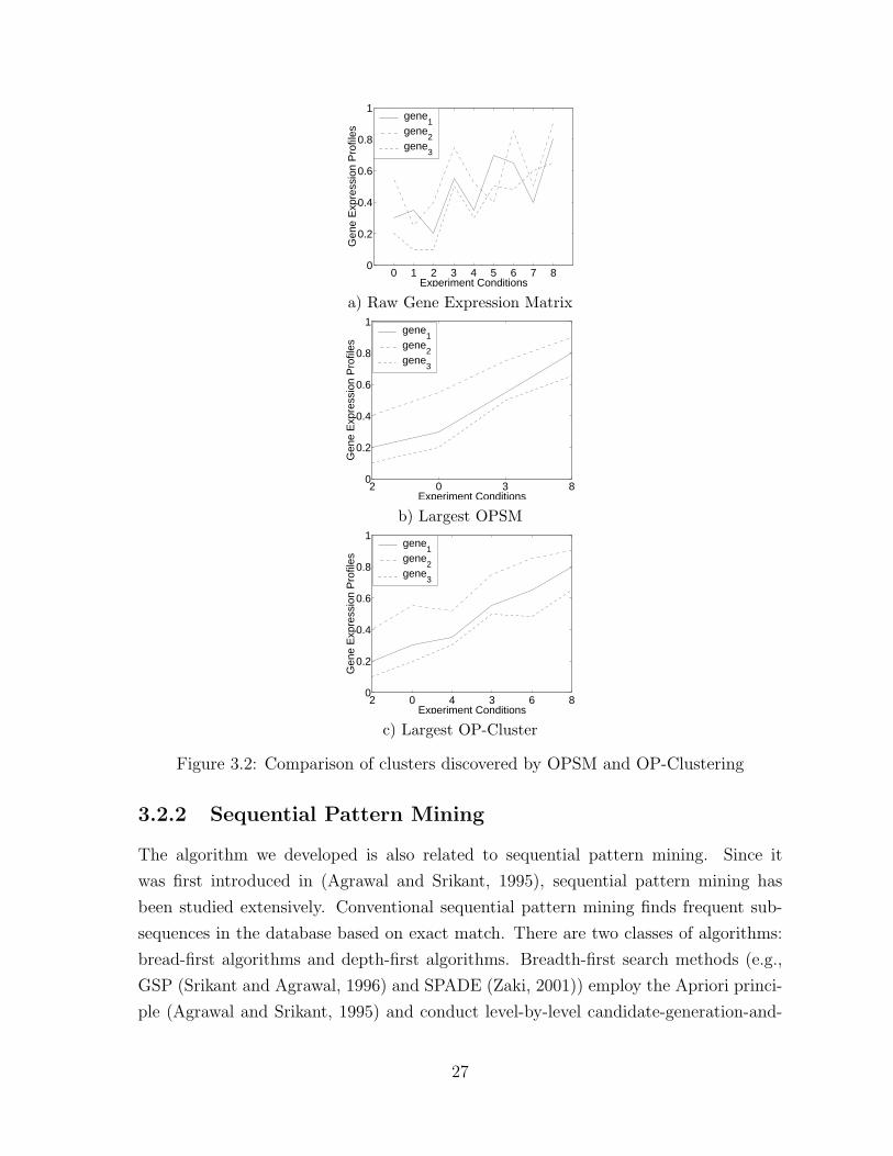
0 1 2 3 4 5 6 7 80

0.2

0.4

0.6

0.8

1

Experiment Conditions

Gen

e E

xpre

ssio

n P

rofil

es

gene1

gene2

gene3

a) Raw Gene Expression Matrix

2 0 3 80

0.2

0.4

0.6

0.8

1

Experiment Conditions

Gen

e E

xpre

ssio

n P

rofil

es

gene1

gene2

gene3

b) Largest OPSM

2 0 4 3 6 80

0.2

0.4

0.6

0.8

1

Experiment Conditions

Gen

e E

xpre

ssio

n P

rofil

es

gene1

gene2

gene3

c) Largest OP-Cluster

Figure 3.2: Comparison of clusters discovered by OPSM and OP-Clustering

3.2.2 Sequential Pattern Mining

The algorithm we developed is also related to sequential pattern mining. Since it

was first introduced in (Agrawal and Srikant, 1995), sequential pattern mining has

been studied extensively. Conventional sequential pattern mining finds frequent sub-

sequences in the database based on exact match. There are two classes of algorithms:

bread-first algorithms and depth-first algorithms. Breadth-first search methods (e.g.,

GSP (Srikant and Agrawal, 1996) and SPADE (Zaki, 2001)) employ the Apriori princi-

ple (Agrawal and Srikant, 1995) and conduct level-by-level candidate-generation-and-

27

tests. Alternatively, depth-first search methods (e.g., PrefixSpan (Pei et al., 2001)

and SPAM (Ayres et al., 2002)) grow long patterns from short ones by constructing

projected databases.

We are faced with a similar but more complicated problem than sequential pattern

mining. Rows in matrix will be treated as a sequence to find sequential patterns.

However, in order to finally determine OP-Cluster, the ID associated with each sequence

has to be kept during the mining process. A depth-first traversal of the tree is carried

out to generate frequent subsequences by recursively concatenating legible suffixes with

the existing frequent prefixes.

3.3 Model

In this section, we define the OP-Cluster model for mining objects that exhibit tendency

on a set of attributes.

3.3.1 Definitions and Problem Statement

Definition 3.3.1 Let o be an object in the database, 〈do1, do2, ..., dom〉 be the attribute

values in a non-decreasing order, m be the number of attributes and δ be the user

specified threshold. We say that object o is similar on attributes i, i + 1, ..., i + j,

(0 < i ≤ m, 0 < j ≤ m), if

(do(i+j) − doi) < G(δ, doi) (3.1)

we call the set of attributes 〈i, i + 1, ..., i + j〉 a similar group. Attribute doi is called

a pivot point.

The grouping function G(δ, doi) return a difference threshold based on δ and may

or may not be related to doi.

The intuition behind this definition is that, if the difference between the values of

two attributes is not significant, we regard them to be “equivalent” and group them

together. There are multiple ways to define the grouping function G(δ, doi). One way

is to define it as the average difference between every pair of attributes whose values

are closest.

G(δ) = δ ×∑

0<j≤m

(doj+1 − doj) (3.2)

28

This definition is independent of doj and is usually used when each attribute has a

finite domain and its value is uniformly distributed. The previous example on movie

rating belongs to this case. When the value of each attribute follows a skewed dis-

tribution, Equation 3.3 is a better choice. The gene expression data often belongs to

this scenario. For the sake of simplicity in explanation, we assume Equation 3.3 in the

remainder of this paper, unless otherwise specified.

G(δ, doj) = δ × doj. (3.3)

For example, suppose a reviewer’s rates of five movies (A,B,C,D, E) as (1, 4, 4.5,

8, 10). If δ = 0.2, 4 and 4.5 are considered equivalent. The rating are divided into four

groups {{1}, {4, 4.5}, {8}, {10}}.

Definition 3.3.2 Let o be an object in the database, and (go1) (go2)...(gok) be a sequence

of similar groups of o by Equation 3.1 and in non-descending order of their values. o

shows an ’UP’ pattern on an ordered list of attributes a1, a2, ..., aj if a1, a2, ..., aj is a

subsequence of (go1)(go2)...(gok)

In the above example, (1, 4, 4.5, 8, 10) is the rating for movies (A,B, C,D,E). After

we apply the group similarity, we are able to transform the original rating to the

sequence A(BC)DE. ABDE, AE, and (BC)E show ’UP’ patterns.

Definition 3.3.3 let I be a subset of objects in the database, I ⊆ O. Let J be a subset

of attributes A. (I, J) forms a OP-Cluster if there exists a permutation of attributes

in J , on which every object in I shows the same “UP” pattern.

Suppose we have two movie ratings o1 and o2 for movies (A,B,C, D,E). The ratings

are (1, 4, 4.5, 8, 10) and (2, 5, 7, 4.5, 9), respectively. According to Definition 3.3.3, the

corresponding sequence of groups for o1 is A(BC)DE, and for o2 is A(DB)CE. Since

ABCE is a common subsequence of them, we say that o1 and o2 form a OP-Cluster on

the attributes sets of ABCE.

Lemma 3.3.1 Let (Op, T p) be a δ-pCluster, where δp is the user defined threshold for

δ-pCluster. (Op, T p) is also identified as a OP-Cluster if the value difference between

any two attributes of an object is at least δp

2.

Proof 3.3.1 Given any two objects x and y (x, y ⊆ Op), we first sort attribute values

of x for all attributes in T p in non-descending order. Without loss of generality, assume

29

that we have two attributes a and b (a, b ⊆ T p) where dxa < dxb. If dya > dyb and any

two attributes of an object differ in value by at least δp

2, we have

(dxa − dxb) < −δp

2; (dya − dyb) ≥

δp

2; (3.4)

The absolute difference between them, which is pScore defined in δ-pCluster, is

|(dxa − dxb)− (dya − dyb)| > δp. (3.5)

However, because x, y ⊆ Op and a, b ⊆ T p, (Op, T p) forms a δ-pCluster. We should

have

|(dxa − dxb)− (dya − dyb)| < δp. (3.6)

This gives a contradiction between Equations 3.5 and 3.6. Therefore, our hypothesis of

dya > dyb is incorrect. So, we have dya ≤ dyb when dxa < dxb, and hence ({x, y}, {a, b})forms a OP-Cluster.

Similarly, we can prove that any two objects ⊆ Op and any two attributes ⊆ T p

can form a OP-Cluster. Thus, for any two objects, they form a OP-Cluster on all

attributes ⊆ T p. Since there is only one unique order of attributes ⊆ T p such that all

objects ⊆ Op show the ’up’ pattern. We conclude that (Op, T p) is also a OP-Cluster.

In above discussion, we assume that the threshold of group similarity is set to 0.

In this case, if the difference between any two attributes of an object is smaller than

the threshold δp

2, it will be included in δ-pCluster, but it will not be able to present

in OP-Cluster. To accommodate this in OP-Cluster, we can set δ = δp

2. Then, any

δ-pCluster will be included in a OP-Cluster.

Lemma 3.3.2 Given a matrix with size n×m, the probability of finding a submatrix

with size nc× nr is

p(nc, nr) =m!

nc!

n∑i=nr

(n

i

)(

1

nc!)i(1− 1

nc!)n−i (3.7)

The above probability originally discussed in (Ben-Dor et al., 2002)measures the sig-

nificance of a submatrix with size (nc × nr). Hence, given the size of the cluster,

we will be able to determine the significance of cluster. This can be used during the

postprocessing in order to select the most significant clusters.

30

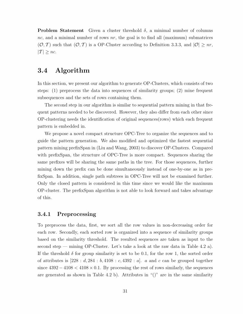
Problem Statement Given a cluster threshold δ, a minimal number of columns

nc, and a minimal number of rows nr, the goal is to find all (maximum) submatrices

(O, T ) such that (O, T ) is a OP-Cluster according to Definition 3.3.3, and |O| ≥ nr,

|T | ≥ nc.

3.4 Algorithm

In this section, we present our algorithm to generate OP-Clusters, which consists of two

steps: (1) preprocess the data into sequences of similarity groups; (2) mine frequent

subsequences and the sets of rows containing them.

The second step in our algorithm is similar to sequential pattern mining in that fre-

quent patterns needed to be discovered. However, they also differ from each other since

OP-clustering needs the identification of original sequences(rows) which each frequent

pattern is embedded in.

We propose a novel compact structure OPC-Tree to organize the sequences and to

guide the pattern generation. We also modified and optimized the fastest sequential

pattern mining prefixSpan in (Liu and Wang, 2003) to discover OP-Clusters. Compared

with prefixSpan, the structure of OPC-Tree is more compact. Sequences sharing the

same prefixes will be sharing the same paths in the tree. For those sequences, further

mining down the prefix can be done simultaneously instead of one-by-one as in pre-

fixSpan. In addition, single path subtrees in OPC-Tree will not be examined further.

Only the closed pattern is considered in this time since we would like the maximum

OP-cluster. The prefixSpan algorithm is not able to look forward and takes advantage

of this.

3.4.1 Preprocessing

To preprocess the data, first, we sort all the row values in non-decreasing order for

each row. Secondly, each sorted row is organized into a sequence of similarity groups

based on the similarity threshold. The resulted sequences are taken as input to the

second step — mining OP-Cluster. Let’s take a look at the raw data in Table 4.2 a).

If the threshold δ for group similarity is set to be 0.1, for the row 1, the sorted order

of attributes is [228 : d, 284 : b, 4108 : c, 4392 : a]. a and c can be grouped together

since 4392− 4108 < 4108× 0.1. By processing the rest of rows similarly, the sequences

are generated as shown in Table 4.2 b). Attributes in “()” are in the same similarity

31

group. Since order in the same groups does not matter, without loss of generality, they

will be arranged in the alphabetical order.

(Equation 3.3).

rID a b c d1 4392 284 4108 2282 401 281 120 2983 401 292 109 2384 280 318 37 2155 2857 285 2576 2266 48 290 224 228

rID sequence1 db(ac)2 c(bd)a3 cdba4 cdab5 dbca6 a(cd)b

a) Raw Data Matrix b) Sequences after Preprocessing

Table 3.1: Example Data Set

3.4.2 OPC-Tree

In the above section, each row in the matrix has been converted into a sequence of col-

umn labels. The goal in the next step is to discover all the frequent subsequence in the

given sequences. This problem seems to be a sequential pattern mining problem, how-

ever,it differs from a conventional sequential pattern mining problem in two respects.

First, the set of rows associated with each frequent subsequence has to be recorded in

order to determine the rows involved in a OP-Cluster. Conventional sequential mining

algorithms only the number of appearance of frequent subsequences. To discover the

set of rows associated with them, one possible approach is to scan database to collect

the related rows. However, this method is very time consuming and is not scalable to

the size of the database. Secondly, our data sets is special. For example, the appear-

ance frequency of each item(column) is the same since each item appears only once

in each sequence. As a result, no pruning happens in the first round of operation in

either apriori-based or projection-based algorithm. Based on the characteristics of our

algorithms, we develop the following algorithm.

Our algorithm uses a compact tree structure to store the crucial information used

in mining OP-Clusters. Meanwhile, sequences sharing the same prefixes are grouped

together. As a result, further operations along the shared prefixes by a set of rows are

only performed once. Pruning techniques can also be applied easily in the OPC-Tree

structure. To make the algorithm more scalable to the number of columns, an improve-

32

ment over OPC-Tree by collapsing nodes in a single paths will be further illustrated in

the OPC-Tree.

Before we define OPC-Tree formally, we first give the following example.

Example 3.4.1 For the sequences in Table 4.2 b), with nc = 3, nr = 3, the OPC-Tree

algorithm performs in the following steps.

Step 1: Create root -1 and insert all the sequences into the tree. This is showed in

Figure 3.3 (1). Notice that same prefix falls on same branch of the tree. The sequence

ID is stored in the leaves. The current root is −1 and the current depth is 0.

Step 2: For each child of the root, insert suffixes in its subtree to the root’s child

that has a matching label. In Figure 3.3 (2), c is a child of the root −1. In this subtree,

the suffix subtree starting at d (for sequence 3, 4) is inserted into the root −1’s child d.

Each insertion is illustrated by a dotted line connecting the two involved nodes, with

the arrow pointing to the destination node in Figure 3.3. The sequence IDs associated

with the suffixes are combined with existing IDs in the destination node. In the case

where a suffix is too short to satisfy current depth + length of the suffix > nc, the

suffix will not be inserted. For example, ba in sequence 3 is also a suffix, it is not to be

inserted because the depth 0 + length of ba < nc.

Step3: Prune current root’s children. If the number of rows falling in a subtree is

smaller than nr, the subtree will be deleted since no further development can generate

a cluster with more than nr rows. For example, subtree leading from −1b in Figure 3.3

(2) is deleted in Figure 3.3 (3) since there are only two sequences falling in this subtree.

Step4: Repeat Step2-Step5 for the root’s first child recursively until there is no child

node left. For example, c is the first child of root-1. Therefore, the same procedure in

step2 is applied to c first. The suffixes of c’s subtree d, such as ba and ab are inserted

into c’s subtree b and a respectively. Since there was less than three sequences fall on

c’s subtrees a and b, the branches −1ca− and −1cb− are deleted. Following the same

procedure, we develop c’s only subtree −1cd−, which is shown in Figure 3.3(4).

Step5: Repeat Step2-Step5 for the root’s next siblings recursively. For example,

after finishing −1c−’s subtree development, the next subtree to develop is −1c−’s

sibling −1d−. −1db’s suffix ac is inserted to subtree −1da. However, both subtrees are

deleted because they do not have sufficient support count.

Definition 3.4.1 OPC-tree (Order Preserving Clustering tree). An OPC-Tree is a tree

structure defined below.

33

-1

c

b

d

a:2

d

b:4

a b

a:3 c:1

a:3

b

db

a

c:1

d

a:2 b:4

a

! Nonr<3

-1

c

b

d

a:2

d

b:4

a:2 b

a:3 c:1

a:3

b

d

b:4

a

b:4

a

a:3

! Nonr<3

! Nonr<3

-1

c

d

b:4

a:2,3

a:3 c:1

a:3

b

d

b:4

a

b:4

! Nonr<3

!Yesnc=3nr=3

-1

c

d

b:4

a:2,3

c:1

a:3

b

d

b:4

a

!Yesnc=3nr=3

-1

c

b

d

a:2

d

b:4

a b

a:3 c:1

a

b

d

Figure 3.3: OPC-Tree for Table 4.2. The label in the oval shape represents the column.The number following ’:’ represents the row ID. The node with double oval meansactive node in the depth first traveral. ’ !No’ means the must-be-pruned subtree. ’Yes’means a valid subtree. A) . Initiate the tree with all the rows B). Insert the suffix of-1’s subtrees to -1’s subtrees. C). Prune the subtree (nr < 3), Insertion. D). Identifythe first E). Finish growing the -1’s first subtree-1a, the next is -1d.

34

1. It consists of one root labeled as ”-1”, a set of subtrees as the children of the root;

2. Each node in the subtrees consists of four entries: entry value, a link to its first

children node, a link to its nearest sibling node, and a link list of all the rows that

share the same path leading from root to this node, but do not have longer subsequences

passing this node. In other words, the sequence IDs are only recorded at the nodes which

marked the end of a subsequence.

Algorithm 1 OPC − Tree(S, nr, nc) newlineInput: S: The sequence set from pre-processing of original Matrix,nr: minimal number of rows, nc: minimal number ofcolumns.Output: All the subsequence with frequency count≥ nr and length ≥ nc.Main program to develop the tree. Create the root of an OPC-Tree, T , and label it as”-1”.

for each sequence s in S doinsertSequence(s, T )growTree(T )

end for

Algorithm 2 insertSequence(s, T )Input:s[i..n]: the sequence to be inserted, T : the root of OPC-TreeOutput:T : tree with the path corresponding to sInsert a sequence into the root of a tree

if i = n theninsert the ID of s into N ’s IDlistreturn

elseif T has a child N such that N.value = s[i].value theninsertSequence(s[i+ 1..n]);N);

elsecreate a new node N .if T ’s first child 6= ∅ then

the last sibling’s next sibling ←N .else

T’s first child ←N .end ifinsertSequence(s[i+ 1..n]);N)

end ifend ifreturn

35

Algorithm 3 growTree(T , nc, nr, depth)Input: T : the root of the initiated tree, nc and nrOutput: OP-Clusterexisted in TGrow patterns based on original T

if T = ∅ thenreturn;

end ifTchild ←T ’s first child;for each sub-tree subT of T do

insertSubTree(subT , T )end forpruneTreeNode(T );growTree(Tchild, nc, nr, depth+ 1);growTree(T ’s next sibling, nc, nr, depth);return.

Analysis of OPC-Tree construction Only one scan of the entire data matrix is

needed to construct an OPC-Tree. For each row, we sort it into a sequence of similarity

groups. Then we insert the sequences into the OPC-Tree. As a result, rows with the

same prefixes share the same paths from root. To save memory, only the row number

associated with each path is recorded at the node corresponding to the end of the

sequence. To find the OP-Cluster using the OPC-Tree, subsequences are developed by

adding suffixes of each sub-tree as the tree’s children, via a pre-order traversal of the

OPC-Tree.

Lemma 3.4.1 Given a matrix M, a similarity grouping threshold, the initiated OPC-

Tree contains all the information of matrix M.

Rationale: Based on the OPC-Tree construction process, each row in the matrix

is mapped onto one path in the OPC-Tree. The row IDs and the order of the columns

are completely stored in the initiated OPC-Tree.

Mining OP-Cluster Using OPC-Tree

Lemma 3.4.2 The developed OPC-Tree on a set of sequences contains all subsequences

hidden in the initial OPC-Tree.

Rationale: Given any sequence S = x1x2x3x4 . . . xn, we want to show that all

subsequences of S will be found in a path starting from root. Through the initiation of

36

OPC-Tree, we know that S will exist in the OPC-Tree. Then given any subsequence

SS = xixj . . . xs, (i ≥ 1, s ≤ n), we can obtain SS by the following steps. First, at node

xi, if i = 1, then insert suffix xixi+1 . . . xn. Now in the subtree of xi, we can find node xj

because it will be along the path xixi+1 . . . xn that is inserted in the first step. Similarly,

we insert the suffix xj . . . xn starting from xj. Now we get the path xixjxj+1 . . . xn. By

repeating the same procedure, a suffix starting with xs is inserted. We get the path

xixj . . . xs. Since we insert all the suffixes in the OPC-Tree, the OPC-Tree contains all

the subsequences presented in the original OPC-Tree.

Rows in a OP-Cluster share the same set of columns, which share the same path

in the OPC-Tree. We can conclude that the OPC-Tree contains all the clusters. This

leads to the following lemma.

Lemma 3.4.3 The developed OPC-Tree on a set of sequences contains all potential

OP-Clusters. The columns in these clusters are on the paths leading from the root to

any tree node with depth no less than nc and row support count in its subtree no less

than nr .

Pruning OPC-Tree

Without any pruning, the whole OPC-Tree fits well into memory when we have a small

matrix (15 columns by 3000 rows). However, for large matrices, some pruning strategies

must be employed to minimize the size of the OPC-Tree. There are two useful pruning

techniques. One strategy is to prune the suffixes with the to-be subsequence shorter

than nc; the other is to prune the subtrees where the row support count is below nr.

Lemma 3.4.4 For a node N in OPC-Tree with depth d, and for a suffix S with length

l in its sub-tree, if d+ l < nc (the minimum columns required for a cluster), this suffix

S will not be useful in forming any OP-Cluster cluster.

Rationale: The length of the path L generates by combining the path from root to N

and S is d+ l. Based on Lemma 3.4.3, L will not form any cluster. Therefore, suffix S

need not be inserted. In our implementation, we check depth of the node at which the

end of the suffix is inserted. If the depth is smaller than nc, the row IDs recorded in

this node will be deleted.

37

-1

c

bda:2

d

ab:4

dbac:1b

a:3

-1

c

d

c:1

db

! Nonr<3

ba:3

ab:4b

a:3

ab:4

bda:2

da:2

ac:1

-1

c

b d

a:3

! Nonr<3

! Nonr<3

c:1

d

ba:3

ab:4b

a:3

ab:4 d

a:2 b:4

a:2

Figure 3.4: Collapsing OPC-Tree for Table 4.2. Sequences in the large vertical ovalmeans collapsed nodes

38

3.4.3 Improvement with Collapsing Node

The major cost of OPC-Tree development is to concatenate suffix trees to existing

prefixes. To minimize the memory footprint, we introduc a more compact OP-Cluster

structure, in which single-path tree can collapse into one node.

Figure 3.4 shows the procedure to construct collapsed OP-Cluster structure for the

same problem as in Example 3.4.1. All collapsed nodes are denoted by rectangles.

There are two scenarios when collapsed node needs to be split.

• The collapsed node will split if a new branch has to be inserted in the middle of

path. For example, in Figure 3.4, sequence 1 (dbac) is collapsed into one node

when the tree is initiated. In the development of depth 2, since the subsequence

dab in sequence 4 will be inserted into path dbac, and the only common prefix

they have is d, a new branch ab has to be added in d’s sub-tree. The original node

which contains dbac will split into two nodes which contain d and bac respectively.

bac will become a sub-tree of d.

• The collapsed node will split if the inserted branch is a contiguous portion of

the single path in the collapsed node. For example, in Figure 3.4, when the

subsequence dba in sequence 3 is inserted into dbac of sequence 1, dba is a portion

of dbac, dbac is split into two parts dba and c. The number 3 is stored at the end

of dba to record sequence ID correctly.

Compared with the original OPC-Tree, the collapsed OPC-Tree occupies less space

and takes much less time. For example, at depth 0, the original tree needs 15 nodes,

while the collapsed tree only needs 5. At depth 1, the original tree needs 21 nodes, but

collapsed one needs only 12. In addition, with collapsed OPC-Tree, inserting suffix of

single-path tree is avoided.

The single-path is compacted into one collapsed node already. The OP-Cluster can

be identified immediately.

3.4.4 Addition Feature: δ-pCluster

According to Lemma 3.3.1, δ-pCluster can be a special case of OP-Cluster if δ ≥ δp

2.

Therefore, our algorithm for mining OP-Cluster can also be used to find δ-pCluster.

Some experiments along this direction is presented in Section 6.7.

39

3.4.5 Additional Feature: Extension of Grouping Technique

Based on Definition 3.3.1, We can generate different similarity groups if we start from

different pivot attributes. For example, If we have an object with four attributes

[A,B,C,D]. The values for the attributes are [0.5, 1, 1.5, 2]. With the similarity thresh-

old as δ = 100%. We can group them either as (AB)(CD) or as A(BCD). Now have

objects 2 and 3 with attribute values [1, 2, 4, 5] and [9, 4, 5, 6], respectively. Their corre-

sponding group sequences are (AB)(CD) and (BCD)A. If we set nc = 3 and nr = 2,

the cluster we can get is (AB)(CD) if we group object 1 as (AB)(CD). However, if

we use A(BCD), the cluster will be (BCD). And both are valid clusters. To find

them, we propose an alternative grouping approach. We put all (possibly overlapping)

similar groups in one sequence. For example, in the above example, object 1 becomes

A(AB)(BCD)(CD). Then, we can find all sequential patterns of these three objects,

which are (AB)(CD) and (BCD). Since we introduce some redundancy, when one

attribute appears more than once in a final cluster, we remove all duplicates.

3.5 Experiments

We experimented with our OP-Cluster algorithm on two real data sets. The algorithm

was implemented in C and executed on a Linux machine with a 700 MHz CPU and

2G main memory. We also implemented the optimized prefixSpan algorithm for com-

parison. The following tests are organized into three categories. First, we studied the

sensitivity of OP-Cluster to various parameters. Secondly, we evaluated the perfor-

mance of OPC-Tree and compared it with the prefixSpan algorithm. To conclude, we

show two promising patterns found in the drug activity data set.

3.5.1 Data Sets

We experimented with our OP-Cluster algorithm on two real data sets.

Gene Expression Data

Gene expression data are generated by DNA chips and other microarray techniques.

The yeast microarray contains expression levels of 2,884 genes under 17 conditions (Spell-

man et al., 1998). The data set is presented as a matrix. Each row corresponds to a gene

and each column represents a condition under which the gene is developed. Each entry

40

represents the relative abundance of the mRNA of a gene under a specific condition.

The entry value, derived by scaling and logarithm from the original relative abundance,

is in the range of 0 and 600. Biologists are interested in finding subsets of genes ex-

hibiting similar up-regulation or down-regulation under a subset of conditions (Cheng

and Church, 2000).

Drug Activity Data

Drug activity data is also a matrix with 10000 rows and 30 columns. Each row cor-

responds to a chemical compound and each column represents a descriptor/feature of

the compound. The value of each entry varies from 0 to 1000.

3.5.2 Model Sensitivity Analysis

In this section, we evaluate how the similarity threshold δ and δp influences the number

of clusters and their sizes. We use the yeast data set in this set of experiments. The

minimum number of rows is set to be 30 and the minimum number of columns is 10.

We vary δp from ∞ to 5. Figure 3.5 (a) shows the number the clusters generated and

(b) presents the maximum cluster size.

5 10 20 30 50 1000

1

2

3

4

5

6

7x 10

5

Similarity group threshold δ

Num

ber

of c

lust

ers

δp=∞δp=10δp=5

5 10 20 30 50 1000

1

2

3

4

5

6x 10

4

Similarity group threshold δ

Max

imum

siz

e

δp=∞δp=10δp=5

(a) Total number of clusters as a function (b) Size(#column×#rows) as a functionof similarity threshold of similarity threshold

Figure 3.5: Performance Study: cluster number and cluster size V.S.similarity threshold

OP-Clusters are generated when δp is infinity. As δ increases, the total number

of clusters begins to increase, which implies that more columns are grouped together

and that more rows are sharing the same subsequences. However, when the similarity

threshold is larger than 100%, the total number of clusters decreases. This is because

the overlapped clusters generated by small δ begin to merge into bigger clusters when

41

1000 2000 3000 4000 5000 6000 7000 8000 9000 10000100

200

300

400

500

600

700

800

Res

pons

e T

ime(

s)

Number of Rows25 30 35 40 45 500

0.2

0.4

0.6

0.8

1

1.2

1.4

1.6

1.8

2x 10

4

Res

pons

e T

ime(

s)

Number of Columns

(a) Scalability with respect to (b) Scalability with respect tonumber of rows number of columns

Figure 3.6: Performance Study: Response time V.S. number of columns and numberof rows

delta increases. Since long subsequence of columns have a higher chance to fall on a

single path, smaller enclosed subsequences are not counted. Thus, the total number

of clusters decreases. Figure 3.5(b) shows that the maximum size of the OP-Cluster

increases dramatically in this case.

As δp decreases, large clusters tends to split into smaller ones and the total number

of clusters increases. The size of each cluster becomes smaller. When more clusters

with size smaller than nc × nr are eliminated, the total number of clusters restricted

by δp drops below the number of OP-Clusters.

3.5.3 Scalability

We evaluate the performance of the OP-Cluster algorithm as we increase the number of

objects and the number of columns in the data set. The response time of the OPC-Tree

is determined by the size of the tree. Figure 3.6 shows the response time of the drug

activity data set. The columns and the rows of the matrix carry the same significance

in the OP-Cluster model, which is symmetrically defined in Formula 3.1. Although the

algorithm is not entirely symmetric in the sense that it chooses to project column-pairs

first, the curves in Figure 3.6 demonstrate similar trends.

For experiments in Figure 3.6(a), the number of columns is 30. The minimal number

of columns of the embedded OP-Cluster is 9, and the minimal number of rows is set to

0.01N , where N is the number of rows of the drug activity data. The mining algorithm

is invoked with δ = 0.2, nc = 9, and nr = 0.01N . Data sets used in Figure 3.6(b) are

taken from the drug activity data with the number of rows fixed as 1000. The mining

42

2000 3000 4000 5000 6000 7000 800010

20

30

40

50

60

70

80

Number of Rows

Res

pons

e T

ime(

sec)

UPC treeprefixSpan

Figure 3.7: Performance comparison of prefixSpan and UPC-tree

algorithm is invoked with δ = 0.2, nc = 0.66C, and nr = 30.

Figure 3.7 presents the performance comparison between the prefixSpan algorithm

and the OPC-Tree algorithm. In this experiment, we used drug activity data to see

the performance with different number of rows. The parameter setting for this set of

experiment is the following: nc = 9, nr = 0.01N , δ = 0.2. The number of columns

is set to be 20. We observe that the OPC-Tree algorithm constantly outperforms the

prefixSpan algorithm and the advantage becomes more substantial with larger datasets.

Next, we studied the impact of the parameters (δ, nc, and nr) towards the running

time. The results are shown in Figure 3.8. The size of matrix is 27×3776. When nc and

nr are fixed, the running time prolongs when the similarity threshold increases. This is

because the size of the clusters increase as we relax the similarity threshold. Therefore,

the OPC-Tree has to spend more time to construct a deeper tree. When similarity

threshold is fixed, it takes longer time to construct the OPC-Tree as nc decreases. This

is showed in Figure 3.8. According to the pruning techniques we discuss in Lemma

3.4.4, a fewer number of subsequences can be eliminated when using smaller nc. As a

result, a larger tree is constructed, which consumes more time. A similar effect can be

observed with respect to nr from Figure 3.8(b).

3.5.4 Results from Real Data

We applied the OP-Cluster algorithm to the datasets. With parameter δ = 10, Some

interesting clusters are reported in both of the data sets. As showed in Figure 3.9,

the two patterns generated from yeast dataset (Cheng and Church, 2000) present the

coherent tendency along the columns on the Y axis. In Figure 3.9(a), if we rearrange

the columns as 15, 10, 9, 8, 6, 5, 3, 1, we will see the ’up’ pattern embedded in it.

Figure 3.9 (b) shows another interesting cluster which present with a ’down’ tendency

43

21 18 15 120

1000

2000

3000

4000

5000

nc, minimum number of columns

Res

pons

e T

ime(

s)

δ=0.05δ=0.2δ=0.3δ=0.4

20 40 60 100 200

200

400

600

800

1000

1200

1400

1600

nr, minimum number of rows

Res

pons

e T

ime(

s)

δ=0.05δ=0.2δ=0.3δ=0.4

(a) Response time varying similarity (b) Response time varying similaritythreshold and nc threshold and nr

Figure 3.8: Performance Study: Response time V.S. similarity threshold , nc and nr

1 3 5 6 8 9 10 150

50

100

150

200

250

300

350

Columns0 5 7 8 10 11 15

50

100

150

200

250

300

350

Columns

Val

ue

(a) Cluster #1 (b) Cluster #2

Figure 3.9: Cluster Analysis: Two examples OPC-Tree in yeast data

itself. Another pair of patterns are showed in Figure 3.10. They present a series of

consistent patterns under a subset of features. It is also interesting to notice that, the

patterns includes all of three Nars, which is SNar, GNar and HNar.

Besides this, in both of the figures, we observe that the curves with sharper slopes

are discovered with ’up’ pattern, while it can never be discovered by the traditional

distance measure nor other pattern-based models.

3.6 Conclusions

In this chapter, we proposed a new model called OP-Cluster to capture the consistent

tendency clusters exhibited by a subset of dimensions in high dimensional space. In

many applications including collaborative filtering and DNA array analysis, although

44

IAC Qindex Snar Dz Ram Pol VDA0

20

40

60

80

100

120

140

Name of Descriptors

Ent

ry V

alue

AAC Qindex SNar HNar GNar Xt RAM MSD0

2

4

6

8

10

12

14

Name of Descriptors

(a) Cluster #1 (b) Cluster #2

Figure 3.10: Cluster Analysis: Two examples OPC-Tree in drug activity data

the distance (e.g., measured by Euclidean distance or cosine distance) among the objects

may not be close, they can still manifest consistent ’up’ pattern over a permutation

of a subset of dimensions. To address this issue, we introduce a new model called

OP-Cluster to model tendency among a set of objects. We proposed a compact tree

structure, namely OPC-Tree, and devised a depth-first algorithm that can efficiently

and effectively discover all OP-Clusters with a user-specified minimum size.

45

Chapter 4

Ontology Driven Subspace Clustering

This chapter introduces a semi-supervised subspace clustering framework by directly

incorporating partial domain knowledge into clustering process. The algorithm yields

a set of subspace clusters with strong classification implication. During the clustering

process, ontology information is utilized to efficiently prune the exponential search space

of the subspace clustering algorithms. Meanwhile, the algorithm generates automatical

interpretation of the clustering result by mapping the natural hierarchical organized

subspace clusters with significant categorical enrichment onto the ontology hierarchy.

Our experiments on a set of gene expression data using gene ontology demonstrate that

our pruning technique driven by ontology significantly improve the clustering perfor-

mance with minimal degradation of the cluster quality. Meanwhile, many hierarchical

organizations of gene clusters corresponding to a sub-hierarchies in gene ontology were

also successfully captured.

4.1 Introduction

Clustering analysis is purely syntactical in the sense that it does not take advantage

of the existing knowledge in the learning process. Eventually, the most challenging

problem is how to approach the matters of interpretability, i.e. why the objects in a

cluster should be clustered together. In many applications, people may have significant

amount of knowledge on the data set, which are usually utilized to measure the signifi-

cance of a cluster. Traditionally, this knowledge is only used during the postprocessing

step for validation of the clustering results. The following are some examples.

• Gene Expression Profiles. The gene expression profile is represented as a matrix

where each row is a gene and each column is a condition while the corresponding

entry records the expression level of the given gene under the given condition. A

large number of gene expression profile analysis tools have been developed (Wang

et al., 2002; Yang et al., 2002; Liu and Wang, 2003). However, all these work

ignore one fact that there exists an extensive amount knowledge of the genes.

For instance, gene ontology (GO) (ash, ) has been developed to categorize the

relationship among genes. The Gene Ontology(GO) has become a well accepted

standard in organizing the classification categories for genes. The relationships,

such as ’part of’ and ’overlapping’, between any two function groups can be

very sophisticated. Until now, no clustering algorithm can generate the clusters

among which the relationships can similarly model the GO hierarchy. The failure

in resembling the relationships may limit the quality of gene function prediction.

Meanwhile, the existing classification of genes are not taken advantage by any

clustering algorithm in order to improve the clustering quality and interpretabil-

ity. Therefore, GO can be utilized to not only speed up the clustering process,

but also produce more biologically meaningful results.

• Customer Preference Profiles. In a user preference data set, each user (customer)

may rank a set of goods. In reality, various goods are not independent of each

other. For instance, VCR, DVD players, and VCD players are very similar while

they are quite different from clothing and sports equipments. This type of knowl-

edge could be utilized for analyzing the customer preferences.

It would be very beneficial (in both execution time and clustering results) if these

knowledge could be utilized. In this paper, we assume that the domain knowledge is

captured in an ontology. The reason that we choose ontology to represent the domain

knowledge is following. (1) This model is flexible yet powerful to capture the various

degrees of relationship among objects (or attributes). (2) It is used in real applications.

For example, in the bioinformatics community, the GO Consortium was formed to

converge the efforts to make the controlled vocabulary of various genomic databases

about diverse species in such a way that it can show the essential features shared by

all the organisms (ash, ).

We propose a hierarchical framework to directly incorporate the ontology knowledge

into subspace clustering process. Our particular interest lies in searching subspace

clusters that can be well explained by its ontology categories. However, is there a

natural correspondence between the hierarchy of subspace clusters and the hierarchy

of ontology? To answer this question, we give the following example.

47

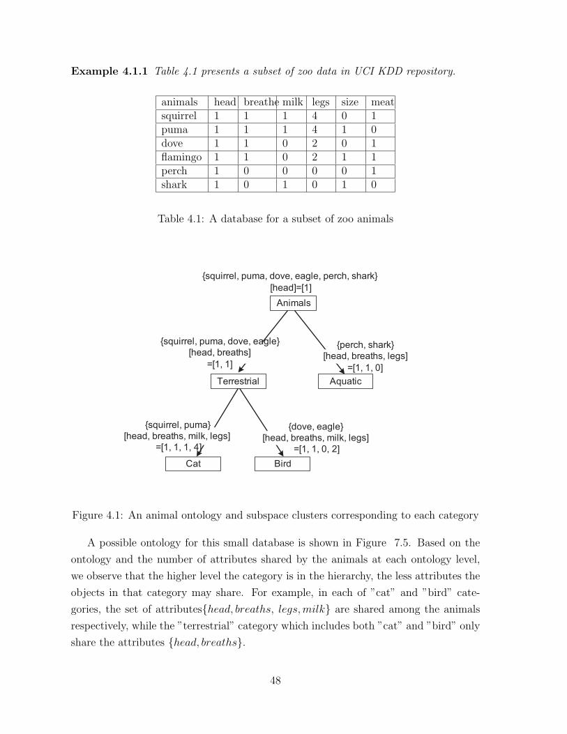
Example 4.1.1 Table 4.1 presents a subset of zoo data in UCI KDD repository.

animals head breathe milk legs size meatsquirrel 1 1 1 4 0 1puma 1 1 1 4 1 0dove 1 1 0 2 0 1flamingo 1 1 0 2 1 1perch 1 0 0 0 0 1shark 1 0 1 0 1 0

Table 4.1: A database for a subset of zoo animals

Animals

{squirrel, puma, dove, eagle, perch, shark}[head]=[1]

Terrestrial

{squirrel, puma, dove, eagle}[head, breaths]

=[1, 1]

Aquatic

{perch, shark}[head, breaths, legs]

=[1, 1, 0]

Cat Bird

{squirrel, puma}[head, breaths, milk, legs]

=[1, 1, 1, 4]

{dove, eagle}[head, breaths, milk, legs]

=[1, 1, 0, 2]

Figure 4.1: An animal ontology and subspace clusters corresponding to each category

A possible ontology for this small database is shown in Figure 7.5. Based on the

ontology and the number of attributes shared by the animals at each ontology level,

we observe that the higher level the category is in the hierarchy, the less attributes the

objects in that category may share. For example, in each of ”cat” and ”bird” cate-

gories, the set of attributes{head, breaths, legs,milk} are shared among the animals

respectively, while the ”terrestrial” category which includes both ”cat” and ”bird” only

share the attributes {head, breaths}.

48

The ontology can not only be used to guide the clustering process, but also can be

used to validate the clustering results. If a cluster contains terms very far apart on

the ontology hierarchy, then the cluster may not be very meaningful in that domain.

According to this example, we may have the following observations of ontology:

• The traditional clustering algorithm might generate the irrelevant clustering result

for classification since some irrelevant attributes might distance the objects that

should be in the same category from each other. For example, while ”puma”

and ”squirrel” are both related to the same category along the attribute set

{head, breaths, legs,milk}, including the other two attributes ”size” and ”meat”

may enlarge the distance between them. Therefore, good clustering result for the

a category may only be located in a subset of attributes.

• Given an ontology hierarchy, it is intuitive that the objects in the higher level of

the category might share less attribute sets than the objects in the lower level of

the hierarchy, as is the case with the animal ontology in Example 4.1.1.

Based on the above observation, given a database with a set of objects featuring

a set of attributes, it will be interesting to find out which subset of objects can be

clustered together over which subset attributes that can be classified into the same

category located in the ontology hierarchy. We also want to find out for each category,

which subset of attributes might contribute to the split of the object sets into more

detailed classification.

We create a general framework for ontology-driven subspace clustering. This frame-

work can be most beneficial for the hierarchically organized subspace clustering algo-

rithm and ontology hierarchy, i.e., it is independent of the clustering algorithms and

ontology application domain. To demonstrate the usefulness of this framework, we

choose TP-cluster algorithm (Liu and Wang, 2003) and the gene ontology as two rep-

resentatives of exhaustive subspace clustering and ontology respectively. Both of them

have been proven useful in clustering gene expression profiles and gene function anno-

tation.

Contribution

• We formally define an ontology hierarchy. Based on this, we use a substructure

of the ontology hierarchy to interpret the categorical meaning of a cluster.

49

• We build a framework to incorporate domain knowledge (represented as ontology)

into subspace clustering. This novel clustering algorithm automatically generates

meaningful clusters (with respect to the ontology) while improving the perfor-

mance.

• We design a new model to assess the objects’ distribution of each ontology cate-

gory in a cluster. Based on this, we developed a ontology-based pruning technique

to minimize the redundancy in the subspace clusters.

• Our experiment results demonstrate that the ontology paths are well corresponded

to certain local structure of hierarchically organized subspace clusters. Mean-

while, the performance of ontology-driven subspace clustering algorithm has great

improvement with minimum loss of clustering quality.

The remainder of this chapter is organized as follows. Section 4.3 defines the model

proposed in the paper. Section 4.4 presents the algorithm in detail. An extensive

performance study is reported in Section 4.5. Section 4.6 concludes the paper and

discusses some future work.

4.2 Ontology Framework

The ontology essentially defines a hierarchy (or DAG) as illustrated in Figure 7.5 where

each node corresponds to a lexion which is the category term. In addition, each term

classified a set of objects and the set of objects in a descendent term is always part of

the set of objects in its ancestor.

Definition 4.2.1 An ontology is a sign system O:=(L,H,R), which consists of

• A lexicon: The lexicon L contains a set of natural language terms.

• A hierarchy H: Terms in L are taxonomically related by the directed , acyclic,

transitive, reflexive relation H. (H ⊂ L×L);

A top term R ∈ L. For all l ∈ L, it holds: H(l,R).

One example of the ontology in Bioinformatics application is Gene Ontology. GO

Consortium was formed to integrate the efforts to make the controlled vocabulary of

various genomic databases about diverse species in such a way that it can show the

50

essential features shared by all the organisms (ash, ). GO has three ontology files

corresponding to its three categories, namely molecular function, biological process

and cellular component. An acyclic directed graph can be obtained for each category

with GO terms as nodes. The recognition of the GO hierarchical system as a diagraph

with top-down directions makes us easily catch the structure of the ontology. Figure 4.2

presents a screen shot of the top levels of the gene ontology. At the first level, genes are

divided into three categories, i.e., Molecular Function(MF), Cellular Component(CC)

and Biological Process(BP).

Figure 4.2: Schema of GO annotation terms.

Formally, GO hierarchy is naturally described as a directed acyclic graph (DAG).

GO =< V , E >, where V is a set of gene function description (GO terms) and E is

a binary relation on V such that genes with functions described by vj are a subset of

genes with functions described by vi, denoted vj � vi, if and only if there exists a path

(vi, vi+1 , ..., vj−1, vj) such that (vm−1, vm) ∈ E for m = i + 1, i + 2, ..., j − 1, j. The

relationship between the children terms and the parent term is also called ”part of” or

”specific”, which means that all the genes annotated as the children GO terms will also

be included as part of the genes annotated as the parent GO term.

Nevertheless, to fit GO in our model, we will transform the original digraph of GO

into our desired form, an ordered tree that is a directed tree with an order defined for

siblings. Note that the same GO term may occur several times (in different lines) in

an ontology file. From a biological viewpoint, these occurrences should be considered

51

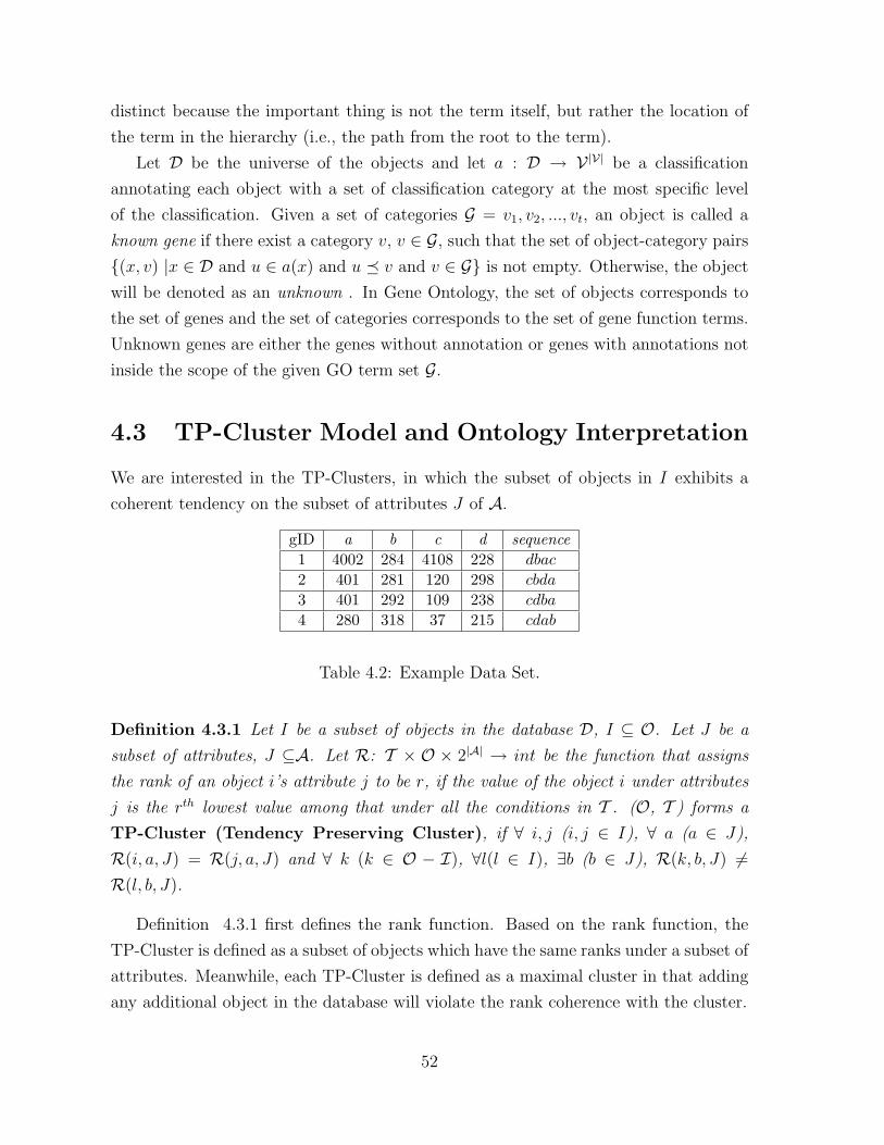
distinct because the important thing is not the term itself, but rather the location of

the term in the hierarchy (i.e., the path from the root to the term).

Let D be the universe of the objects and let a : D → V |V| be a classification

annotating each object with a set of classification category at the most specific level

of the classification. Given a set of categories G = v1, v2, ..., vt, an object is called a

known gene if there exist a category v, v ∈ G, such that the set of object-category pairs

{(x, v) |x ∈ D and u ∈ a(x) and u � v and v ∈ G} is not empty. Otherwise, the object

will be denoted as an unknown . In Gene Ontology, the set of objects corresponds to

the set of genes and the set of categories corresponds to the set of gene function terms.

Unknown genes are either the genes without annotation or genes with annotations not

inside the scope of the given GO term set G.

4.3 TP-Cluster Model and Ontology Interpretation

We are interested in the TP-Clusters, in which the subset of objects in I exhibits a

coherent tendency on the subset of attributes J of A.

gID a b c d sequence1 4002 284 4108 228 dbac

2 401 281 120 298 cbda

3 401 292 109 238 cdba

4 280 318 37 215 cdab

Table 4.2: Example Data Set.

Definition 4.3.1 Let I be a subset of objects in the database D, I ⊆ O. Let J be a

subset of attributes, J ⊆A. Let R: T × O × 2|A| → int be the function that assigns

the rank of an object i’s attribute j to be r, if the value of the object i under attributes

j is the rth lowest value among that under all the conditions in T . (O, T ) forms a

TP-Cluster (Tendency Preserving Cluster), if ∀ i, j (i, j ∈ I), ∀ a (a ∈ J),

R(i, a, J) = R(j, a, J) and ∀ k (k ∈ O − I), ∀l(l ∈ I), ∃b (b ∈ J), R(k, b, J) 6=R(l, b, J).

Definition 4.3.1 first defines the rank function. Based on the rank function, the

TP-Cluster is defined as a subset of objects which have the same ranks under a subset of

attributes. Meanwhile, each TP-Cluster is defined as a maximal cluster in that adding

any additional object in the database will violate the rank coherence with the cluster.

52

For example, in Table 4.2, we say that the gene set {2, 3} forms a cluster along the

subset of conditions {a, c, d}, since the ranks of the three conditions for both genes are

the same, i.e. (3, 1, 2).

Next,we show that each TP-Cluster can be mapped onto an ordered sequence of

condition labels by choosing a consistent order of the conditions in any of the TP-

Clusters, such as monotonically increasing or decreasing.

Definition 4.3.2 Given a TP-Cluster C with object set O and condition set T , We

call a sequence of conditions S representing C in a monotonically increasing order, if

S=π(T ), where function π places each condition a in T at the position R(a) in sequence

S.

For example, for cluster {2, 3}×{a, c, d} in Table 4.2, the sequence of conditions

that represents the monotonically increasing order is cda. For condition c, its rank is 1

and the position in the sequence is 1. It is also the increasing order of the sequence of

conditions

Definition 4.3.3 Given two TP-Cluster C1 and C2 with condition set T1 and T2 respec-

tively, we call C1 is the ancestor of C2 if π(T1) is a prefix of sequence π(T2).

For example in Table 4.2, the sequence representing cluster C1={2, 3}×{a, c, d} is

cda. The sequence representing cluster C2={2, 3, 4}×{c, d} is cd. Since cd is the prefix

of cda, we call C2 is the ancestor cluster of C1.Based on the mapping from TP-Cluster to the sequences, we are able to organize

the TP-Clusters into a prefix tree. We will introduce an algorithm which builds the

HTP-clustering tree in a very compact fashion in the Section 4.4.

The following Lemma present the ’part-of’ relationships of the TP-Clusters.

Lemma 4.3.1 Let C and C ′ be two TP-Clusters in the database D. Let I and I be the

object sets of C and C ′ respectively, if C ′ is the ancestor of C, then I ⊆ I ′.

Proof 4.3.1 Since C ′ is ancestor of C, π(J ′) must be a prefix of π(J), based on Defini-

tion 4.3.3. ∀i(i ∈ I), i supports πJ . Thus, g must support any prefix of πJ . Therefore,

i supports π(J ′), i ∈ I ′. Since ∀i, i ∈ I implies i ∈ I ′, we have I ⊆ I ′.

Obviously, cluster C1 and C2 follows this property. C2 is the ancestor of C1 and

{2, 3, 4}⊇{2, 3}.

53

4.3.1 The HTP-clustering tree

In this section, we will introduce the HTP-clustering tree.

The ODTP-clustering is generally analogous to a prefix tree of a predefined set of

sequences. However, it is also different because of its unique interpretation of each

node and the parent-child relationship. Each node in HTP-clustering tree represents a

unique TP-Cluster.The root node corresponds to the null space. The nodes at level m

correspond to m dimensional TP-Cluster. The TP-Cluster at a node is related to its

immediate parent by being part of cluster. Each TP-Cluster other than the null root

is 1-dimensional extension of its parent cluster. In order to elucidate HTP-clustering

tree we give a maximal TP-Cluster tree of three conditions in Figure 4.3, where each

TP-Cluster is represented by a sequence. We call it ’maximal’ since there does not

exist another TP-Cluster that may not be included in the lattice given the condition

set. The figure contains a three-level tree structure which corresponds to 1-, 2- and

3-dimensional TP-Clusters. Each node u in the HTP-clustering tree is represented by

the path from the root of the TP-Cluster leading to u. For example, the TP-Cluster

with two conditions {b, c} ordered increasingly as (bc) will be put at the node −(∅)bc.The gene set associated with each node in the HTP-clustering tree is not shown in the

figure.

Definition 4.3.4 The HTP-clustering tree is a hierarchical arrangement of TP-Clusters

with the following properties: 1) The tree is rooted at level 0 with ∅. (2) Each node at

level m corresponds to a m-dimensional TP-Cluster represented by a length-m sequence.

2) Each node at level (m + 1) is a 1-dimensional extension of its immediate ancestor,

which corresponds to a length (m+ 1) sequence.

The problem we are interested here is the hierarchical relationship among TP-

Clusters. Investigating the relationships among TP-Clusters may help us with the

prediction of the behavior of higher dimensional clusters based on the lower dimensional

ones.

4.3.2 Annotation of a Cluster

In this subsection, we present the annotation of a cluster given an ontology. We first

introduce the P-value to assess the significance of a particular category within a cluster.

The hypergeometric distribution is used to model the probability of observing at

least k objects from a cluster of g objects by chance in a category containing f objects

54

a b c

ab ac ba bc cb ca

abc acb bac bca cba cab

NULL

Figure 4.3: The maximal hierarchy of the TP-Clusters given a condition spaceA={a, b, c}.

from a total set of n genes. The P-value is given by P = 1 −∑k

i=0

(fi)(

n−fg−i)

(ng)

. The test

measures whether a cluster is enriched with genes from a particular category to a greater

extent than that would be expected by chance. For example, if the majority of genes

in a cluster appear from one category, then it is unlikely that this happens by chance

and the category’s P-value would be close to 0. Adopting the Bonferroni correction

for multiple independent hypotheses, 0.01Na

is used as the threshold θp, to measure the

significance of the P-value.

To annotate a cluster, the P-value of each category present in the cluster will be

computed first. Given a cut-off P-value threshold, categories which have relatively large

P-value will be dropped without further consideration. The result is a set of significant

categories V={v1, v2, ..., vt}. There are two naive ways to annotate the clusters with the

set of the significant categories V . One method is to keep all the significant categories as

annotation candidates. The disadvantage of this one is that it will be hard to determine

the object categories when being assigned to too many functionalities. The other way is

to annotate a cluster with the category that has the least P-value. Choosing the most

significant category to represent the cluster is reasonable. However, it may discard

some important information, such as the significance of the subcategories of the most

significant category.

In our method, we adopt a middle way between the two methods. We use an

appropriate subtree in the ontology to represent the cluster annotation. The subtree

is rooted at the node of the most significant category and includes all the significant

categories that are located in the root’s subtree. The annotation is formally defined as

55

Cell Growthlog(P-value)=-7

Cell Expansionlog(P-value)=-3

Regulation of Cell Growthlog(P-value)=-3

Cell Communicationlog(P-value)=-2

Cellular Processlog(P-value)=-3

Figure 4.4: An example of OST representing a Cluster. The two values in each noderepresent the function category and its P-value.

the Ontology SubTree(OST ) in Definition 4.3.5

Definition 4.3.5 Given a cluster C, and its significant function categories V = {v1, v2, ...vt},Ontology SubTree(OST ) representing a cluster is defined as a tree H. The root of H is

the category vr, 0 < r≤t, where P (vr, C) = min0<i≤t(P (vi, C)). The descendants of Hare the set of the categories which are the immediate descendants of vr in the ontology.

First, with the level-wise structure of ontology, a gene that is classified into a certain

category will always be a member in its ancestor’s category. Therefore, the OST

is rooted at most significant category to ignore the less detailed ancestor function

categories.

Secondly, although the children of v are not as significant as v in cluster C, it is

still possible that later split of the cluster may signify the coherence of the children

categories of v. Thus, we keep these function categories for further clustering.

Figure 4.4 show an OST that annotates a cluster. To determine the OST repre-

senting this cluster, we first find out the location of most significant function groups,

which in this case, is cell growth,with log(P − value)=-7. We then discard its parent

category of cellular process, and siblings, cell communication, which has less P-value.

The resulting OST is the subtree rooted at cell growth.

Definition 4.3.6 Given a cluster C, we call C is functionally enriched if there exists

an OST representing the cluster, given a P-value threshold θp.

Definition 4.3.7 defines the ≺ relationship between two OST s.

56

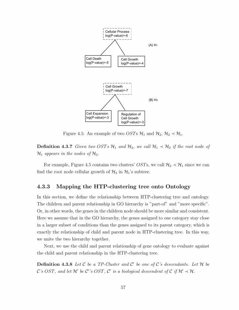
Cellular Processlog(P-value)=-6

Cell Deathlog(P-value)=-5

Cell Growthlog(P-value)=-4

(A) H1

Cell Growthlog(P-value)=-7

Cell Expansionlog(P-value)=-3

Regulation of Cell Growthlog(P-value)=-3

(B) H2

Figure 4.5: An example of two OST s H1 and H2, H2 ≺ H1.

Definition 4.3.7 Given two OST s H1 and H2, we call H1 ≺ H2 if the root node of

H1 appears in the nodes of H2.

For example, Figure 4.5 contains two clusters’ OST s, we call H2 ≺ H1 since we can

find the root node cellular growth of H2 in H1’s subtree.

4.3.3 Mapping the HTP-clustering tree onto Ontology

In this section, we define the relationship between HTP-clustering tree and ontology.

The children and parent relationship in GO hierarchy is ”part-of” and ”more specific”.

Or, in other words, the genes in the children node should be more similar and consistent.

Here we assume that in the GO hierarchy, the genes assigned to one category stay close

in a larger subset of conditions than the genes assigned to its parent category, which is

exactly the relationship of child and parent node in HTP-clustering tree. In this way,

we unite the two hierarchy together.

Next, we use the child and parent relationship of gene ontology to evaluate against

the child and parent relationship in the HTP-clustering tree.

Definition 4.3.8 Let C be a TP-Cluster and C ′ be one of C’s descendants. Let H be

C’s OST , and let H′ be C ′’s OST , C ′ is a biological descendent of C if H′ ≺ H.

57

If the cluster C1 represented by H1 in Figure 4.5 is immediate ancestor of the cluster

C2 represented by H2, we call C2 is the biological descendent of C1 if C1 is its ancestor.

Problem Statement Let D be a database with a set of objects O and condition set

A. Given a threshold θp for cluster enrichment, our goal is to extract a biologically

relevant hierarchy of enriched TP-Clusters.

4.4 Construction of Ontology Relevant HTP-clustering

tree

4.4.1 Construction of HTP-clustering tree

In this section, we show the HTP-clustering tree can be constructed by suffix con-

catenation in conjunction with extracting only biologically relevant TP-Clusters. The

inputs to the HTP-clustering tree construction algorithm include the database D, the

GO ontology, and function enrichment threshold θp. The HTP-clustering tree is con-

structed hierarchically in a top-down fashion, along which the dataset D is partitioned.

The HTP-clustering tree construction uses a depth-first pre-order traversal algorithm

in order to build the tree structure. We prefer the depth-first order to the breadth-first

order because we can minimize the amount of storage needed for each level to develop

clusters in the next level. The depth-first traversal is also correct because for each node,

the construction of its subtree will be relatively independent of the construction of its

siblings.

The HTP-clustering tree construction process can be summarized in two steps:

1. We first preprocess the data. Each row in the data matrix will be converted to

an ordered sequence of column labels based on rank in Definition 4.3.1. Those

sequences will be the inputs to the next steps. An initial prefix tree containing

the sequence of every gene in the database will be constructed.

2. The initial prefix tree will be recursively visited and developed in the depth-

first order to reveal all frequent subsequences, which represent TP-Clusters. The

ontology information of the genes in the database will be fed into the HTP-

clustering tree at the root level. Ontology-based pruning will be performed upon

the visit at each node.

58

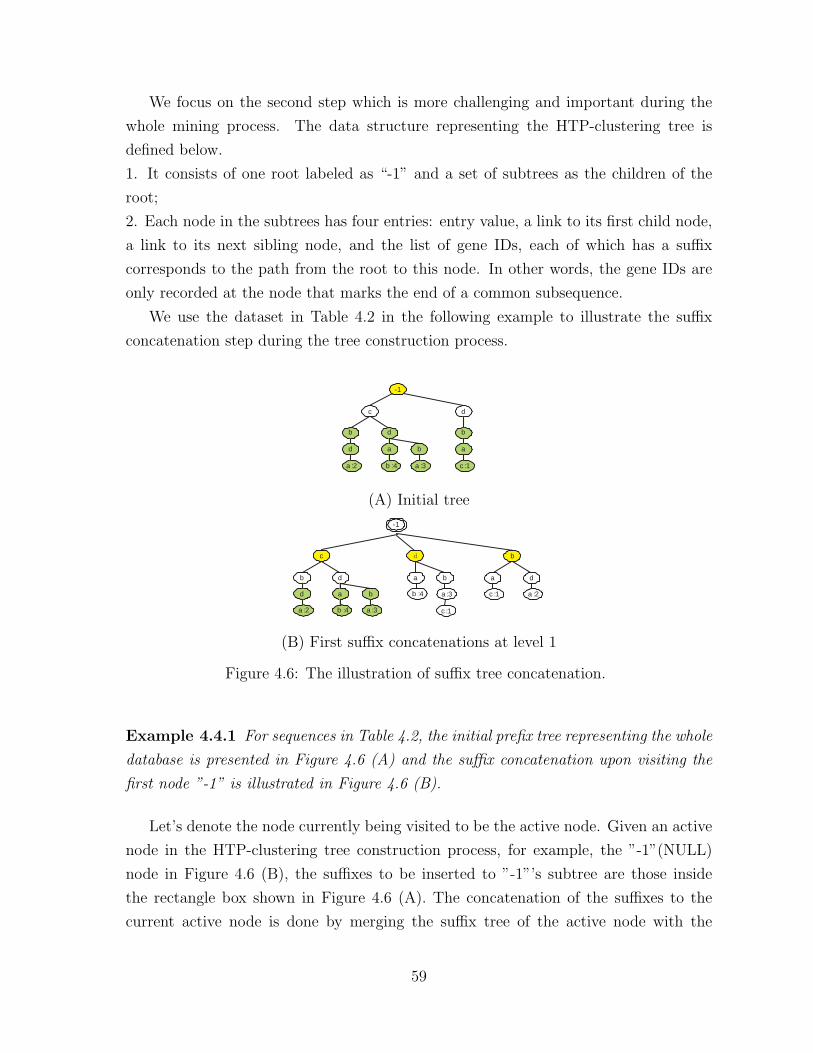
We focus on the second step which is more challenging and important during the

whole mining process. The data structure representing the HTP-clustering tree is

defined below.

1. It consists of one root labeled as “-1” and a set of subtrees as the children of the

root;

2. Each node in the subtrees has four entries: entry value, a link to its first child node,

a link to its next sibling node, and the list of gene IDs, each of which has a suffix

corresponds to the path from the root to this node. In other words, the gene IDs are

only recorded at the node that marks the end of a common subsequence.

We use the dataset in Table 4.2 in the following example to illustrate the suffix

concatenation step during the tree construction process.

��

�

�

�

� ��

�

� ��

� �

� �� � ��

�

�

�

(A) Initial tree

��

�

�

�

� ��

�

� ��

� �

� �� � ��

� ��

�

d �

�

� ��

�

� ��� ��

�

(B) First suffix concatenations at level 1

Figure 4.6: The illustration of suffix tree concatenation.

Example 4.4.1 For sequences in Table 4.2, the initial prefix tree representing the whole

database is presented in Figure 4.6 (A) and the suffix concatenation upon visiting the

first node ”-1” is illustrated in Figure 4.6 (B).

Let’s denote the node currently being visited to be the active node. Given an active

node in the HTP-clustering tree construction process, for example, the ”-1”(NULL)

node in Figure 4.6 (B), the suffixes to be inserted to ”-1”’s subtree are those inside

the rectangle box shown in Figure 4.6 (A). The concatenation of the suffixes to the

current active node is done by merging the suffix tree of the active node with the

59

corresponding subtree one level below the active node. For example, suffix tree ”-1cd”

in (A) is merged with ”-1d”. The generated subtree is shown as the ”-1d” subtree in

(B). (B) is the subsequent tree after the visit of the node ”-1”. The same procedure

will be applied recursively in the depth-first order to construct the HTP-clustering tree.

For example, after the first node visit at the root ”−1”, the next node to be visited

will be ”-1c”, the suffix inside the rectangle box in Figure 4.6(B) will be the next set

of suffixes to be inserted. The TP-Cluster algorithm without biological assessment is

presented in Algorithm 4.

Algorithm 4 g

rowTree(H, depth)Input: H: the root of the initial tree,Output: TP-Cluster existed in HGrow patterns on the initial TP-Cluster H

if tree H = ∅ thenreturn

end ifHchild = H’s first child;for each sub-tree subH of H do

insertSubTree(subH, H);end forgrowTree(Hchild,depth+ 1);growTree(H’s next sibling,depth);

The correctness of HTP-clustering tree construction is proved in Lemma 4.4.1.

Lemma 4.4.1 Given a database D, the HTP-clustering tree contains all the TP-Clusters

embedded in the database.

Rationale: According to Definition 4.3.2, each TP-Cluster corresponds to a unique

sequence of the conditions. Therefore, the proof of the Lemma is equivalent to the the

proof that the HTP-clustering tree contains all the frequent subsequences of the set of

sequences representing rows in the database. Given any subsequence S ′, we want to

prove that all the sequences containing S ′ will be projected onto the path corresponds

to S ′. Given any sequence S = x1x2x3x4 . . . xn, we want to show that all subsequences

of S can be found in a path starting from the root. S is inserted into the tree during

the initiation procedure. Then given any subsequence SS = xixj . . . xs, (1 ≤ i, s ≤ n),

we can obtain SS by the following steps. First, at node xi, insert suffix xixi+1 . . . xn.

Now in the subtree of xi, node xj can be found because it should be along the path

60

xixi+1 . . . xn that is inserted in the first step. Similarly, we insert the suffix xj . . . xn.

As a result, we get the path xixjxj+1 . . . xn. By repeating the same procedure until we

insert the suffix starting with xs, we get the path xixj . . . xs. Since the path representing

a subsequence is unique, all the sequences contain S ′ will fall on the node corresponds

to S ′. The HTP-clustering tree contains all the subsequences, or, in other words, TP-

Clusters.

4.4.2 Ontology Based Pruning Techniques

Several pruning techniques based on the ontology are discussed here. The first pruning

technique we will discuss is the functional distribution pruning. For any cluster C,we expect that there exists at least one function category in C that is statistically

significant. Given a cluster C and the distribution of categories, we use the following

Lemma for early detection of the potential appearance of significant function categories.

Lemma 4.4.2 Let C be a cluster, let V={v1, v2, ..., vt} be a set of function categories

and let S be a counter vector in which si records the number of objects appearing in Cin category vi. Let the minimum number of objects required in a cluster to be nr and

let θp to be P-value threshold. ∀vi, vi ∈ V, Let Ci’ be a cluster with size nr and contains

min(si,nr) objects in category vi. If ∀ i, P (si, Ci′) > θp, then C will not become an

enriched cluster.

Proof 4.4.1 ∀vi, vi ∈ V, we have P (si, Ci′) < P (si, C) based on the property of P-

value, i.e, the P-value increases as the number of objects in the same cluster increases.

According to the condition in the Lemma, we have θp < C ′i < P (si, C). This implies that

∀vi, vi ∈ V, Ci′) < P (si, C). Therefore, according to Definition 4.3.6, C is not enriched

by a particular category.

The second technique is to use OST extracted in a parent cluster to guide the

selection of its descendent clusters, by favoring biological children clusters defined in

Definition 4.3.8. Our criterion are based on the assumption that, the TP-Clusters in

the higher dimensional space will be enriched in the more specific categories.

Criterion 4.4.1 Let C and C ′ be two clusters and C is the parent of C ′ in the TP-Cluster

hierarchy. We say the development of C ′ is not eligible if OSTC′<OSTC.

Combining the two pruning techniques, we apply the following procedure at each

node of the traversal.

61

1. Evaluate the prediction potential of the cluster corresponding to this node. If it

has no potential become a functionally enriched clusters= based on Lemma 4.4.1,

stop further development of this node and its descendants, then go to the next

node in the order of the traversal. If it is not, go to step 2.

2. Extract OST of the cluster. If OST is not biologically eligible according to

Criteria 4.4.1 stop further development of this node and its descendants. Go to

the next node in the order of the traversal.

We present the algorithm of extracting the biologically relevant TP-Clusters by

ODTP-clustering tree in Algorithm 5. Its major differences from the pure tree con-

struction algorithm is the recursively feeding and pruning of OST structure and cluster

evaluation and pruning based on the significance of OST .

Algorithm 5 growTree(H, nc, nr, depth, parentOST )Input: H: the root of the initial tree,Output: TP-Cluster existed in H, original OSTGrow patterns on the initial TP-Cluster H

if H = emptyset thenreturn;

end ifHchild = H’s first child;for each sub-tree subH of H do

insertSubTree(subH, H);end forcurOST= extractOST(H);if curOST is not empty then

if curOST≺parentOST thengrowTree(Hchild, nc, nr, depth+ 1, curOST );

elsegrowTree(Hsib, nc, nr, depth+ 1, parentOST );

end ifelsepotential = evalFunction(H, parentOST )if potential = good then

growTree(Hchild, nc, nr, depth+ 1, curOST );else

growTree(Hsib, nc, nr, depth, parentOST );end if

end if

62

Analysis of HTP-clustering tree and ODTP-clustering tree construction

For both HTP-clustering tree and ODTP-clustering tree, only one scan of the entire

data matrix is needed during the construction. Each row is converted into a sequence

of column labels. The sequences are then inserted into the prefix tree. In the initial

tree structure, sequences with the same prefix naturally fall onto the same path from

the root to the node corresponding to the end of prefix. To save memory, the row IDs

associated with each path are only recorded at the node marking the end of the longest

common prefix shared by these sequences.

Both the time and space complexity of the two algorithms are determined by the

potential size of TP-Clusters. In the worst case scenario, given a gene expression matrix

n ×m, the size of tree is∑m

s=1 s!(

ms

). However, since we use the depth-first traversal

of the tree and the part of tree that has been traversed will not be needed for future

mining, they can be deleted and the space can be reused. At level i, i 6= 0, we only

need to keep m− i+ 1 nodes. Therefore, the maximal space to be allocated during the

running time will be limited to O(n∑m

i=1m− i+ 1) = O(n ∗m2).

ODTP-clustering tree will be more space and time efficient than HTP-clustering

tree in that it uses Ontology information to prune the exponential search space of

HTP-clustering tree construction. The effective of the pruning is largely determined

by the percentage of objects with the same categorization can be clustered together.

4.5 Evaluation

In this section, we use a real dataset to evaluate our algorithm. The dataset is the

yeast cell cycle data from Spellman et al.(Spellman et al., 1998). Our experiments

demonstrate the usefulness of ODTP-clustering algorithm in clustering biologically re-

lated genes with effective pruning techniques based on gene ontology. The results are

evaluated against the mapping between gene ontology and HTP-clustering tree. The

algorithm was implemented in C and executed on a Linux machine with a 700 MHz

CPU and 2G main memory.

The HTP-clustering algorithm is tested on the yeast cell cycle data of Spellman et

al.(1998). The study monitored the expression levels of 6,218 S. cerevisiae putative gene

transcripts (genes) measured at 10-minute intervals over two cell cycles (160 minutes)

with 18 time points. Spellman et al. identified 799 genes that are cell cycle regulated.

We used the expression levels of the 799 genes across 18 time points as the original

input matrix. The HTP-clustering procedure groups together genes on the basis of

63

their common expression tendency across a subset of time points.

To assess the classification capability of the clusters, we map gene ontology infor-

mation to each gene to evaluate whether the cluster has significant enrichment of one

or more function groups. The ontology of the 799 yeast genes is downloaded from gene

ontology consortium (ash, ) in Feb, 2004. We use functions from the three categories:

molecular function, cell component and biological process. We extract categories be-

tween ontology level 2 and level 5 with a family size of at least 5. The discovered

TP-Clusters in each level of the hierarchy are evaluated for enrichment with any of

those function categories.

Types #Knowngenes

#Categories(> 5)

#Annoper gene

MF 370 16 0.77CC 616 48 3.4BP 538 38 5.72

Table 4.3: Statistics for the three categories.

20 30 40 50 60 7040

50

60

70

80

90

100

110

120

130

140

NR

Res

pons

e T

ime(

s)

Pθ=10−3

Pθ=10−4

Pθ=10−5

Pθ=10−6

Pθ=10−7

−3 −4 −5 −6 −70

0.05

0.1

0.15

0.2

0.25

0.3

0.35

0.4

0.45

0.5

log(Pθ)

Per

cent

age

OST−PruningEnrichedPoorFunction

a) Response Time b) The distribution of the clusters

Figure 4.7: The performance of the ODTP-clustering varying nr and θp.

4.5.1 Performance Evaluation

The first set of experiment was done using the ODTP-clustering algorithm and cellular

component ontology to evaluate the performance under various parameters nr and

θp. As shown in Figure 4.7 a), the response time of the ODTP-clustering algorithm

64

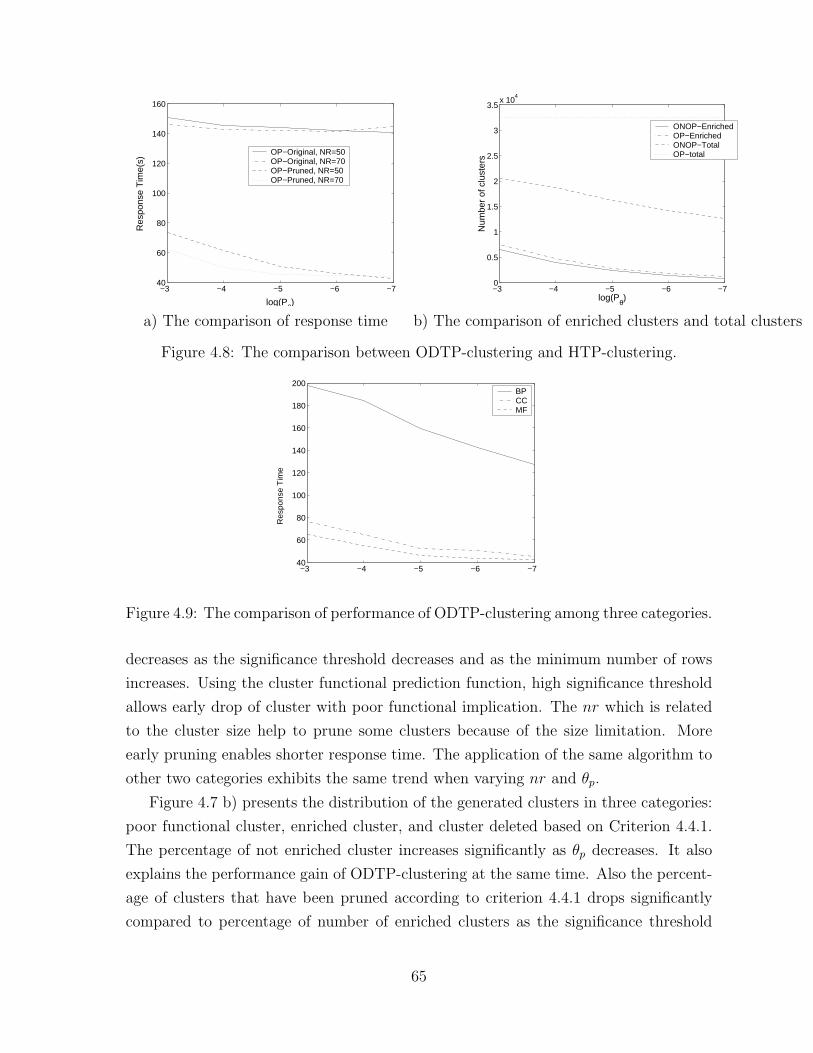
−3 −4 −5 −6 −740

60

80

100

120

140

160

log(Pθ)

Res

pons

e T

ime(

s)OP−Original, NR=50OP−Original, NR=70OP−Pruned, NR=50OP−Pruned, NR=70

−3 −4 −5 −6 −70

0.5

1

1.5

2

2.5

3

3.5x 10

4

log(Pθ)

Num

ber

of c

lust

ers

ONOP−EnrichedOP−EnrichedONOP−TotalOP−total

a) The comparison of response time b) The comparison of enriched clusters and total clusters

Figure 4.8: The comparison between ODTP-clustering and HTP-clustering.

−3 −4 −5 −6 −740

60

80

100

120

140

160

180

200

Res

pons

e T

ime

BPCCMF

Figure 4.9: The comparison of performance of ODTP-clustering among three categories.

decreases as the significance threshold decreases and as the minimum number of rows

increases. Using the cluster functional prediction function, high significance threshold

allows early drop of cluster with poor functional implication. The nr which is related

to the cluster size help to prune some clusters because of the size limitation. More

early pruning enables shorter response time. The application of the same algorithm to

other two categories exhibits the same trend when varying nr and θp.

Figure 4.7 b) presents the distribution of the generated clusters in three categories:

poor functional cluster, enriched cluster, and cluster deleted based on Criterion 4.4.1.

The percentage of not enriched cluster increases significantly as θp decreases. It also

explains the performance gain of ODTP-clustering at the same time. Also the percent-

age of clusters that have been pruned according to criterion 4.4.1 drops significantly

compared to percentage of number of enriched clusters as the significance threshold

65

decreases. This may also indicate that the more significance the enrichment of the

clusters, the more confident that its OST leads to the right direction of selecting the

biologically appropriate subset of conditions.

The second set of experiment in Figure 4.8 a) is a comparison between ODTP-

clustering algorithm and the original clustering algorithm. For each algorithm, we have

done two tests with different setting of nr. We can observe significant and consistent

improvement of ODTP-clustering algorithm over HTP-clustering tree especially when

θp is relatively low. The performance of HTP-clustering can be as short as 1/4 of that

in the original algorithm with appropriate P-value.

Figure 4.8 b) compares the number of enriched clusters and the total number of

clusters. Clearly, the total number of original TP-Clusters remains the same without

ontology based pruning. On the other hand, the total number of clusters using ODTP-

clustering is much smaller than TP-Clusters while the number of enriched TP-Clusters

generated by ODTP-clustering almost stays the same as the number of enriched TP-

Clusters. Overall, ODTP-clustering improves the performance with minimum loss of

categorically enriched clusters.

Figure 4.9 gives the comparison of response time of applying the three different

ontology files. The input parameter for the algorithm is nr=50. We can observe a

clear trend that biological process ontology consistently spends more time than the

rest. The reason behind this can be explained by the data in Table 4.3. The average

number of categories that a gene might have is 5.7, which is much higher than that of

either cellular component or molecular function. With less categories but more gene

annotations, the distribution of function groups in a cluster has higher probability to

be more concentrated in one or more function groups rather than evenly distributed

in any of them. As a result, less functional clusters might be pruned, and hence, the

response time is longer. In addition, this may also be coincident with the hypotheses

that similar gene expression profile may indicate a function relation in biological process

(bro, ). As a result, more time will be taken for generating more enriched significant

clusters compared with the rest two branches in the ontology.

Overall, our experiment shows that ontology-based pruning is effective in reducing

the search space of subspace clustering. In addition, the response time of our algorithm

is determined by the two input parameters and the distribution of genes in each category

in the ontology.

66

4.5.2 Mapping between GO and the HTP-clustering tree

In this section, we present a generic example of hierarchically organized clusters that

map to a hierarchical substructure of GO.

In Figure 4.10, (A) presents a three-level hierarchy of TP-Clusters, while (B) shows

the corresponding OST s. The gene ontology summarizing the relationships among all

the function categories appearing in (B) is ”Necleoside → DNA metabolism → DNA

repair”.

The root cluster C01 in (A) is the largest cluster with 71 genes. However, it has the

least number of conditions shared by all genes in its cluster, i.e. (4, 15, 13, 8). Its OST

shown at the top of the hierarchy in (B) is rooted at the category, Necleoside. As we go

down the hierarchy of clusters in (A), we observe cluster with smaller number of genes

but larger number of consistent conditions. In addition, the OST s tend to exist in the

subtree of the OST in its parent cluster. For example, the root cluster C01 is split

into two smaller overlapping clusters C11 and C12 featuring enriched function ”DNA

metabolism”, which is a subcategories of necleoside. OSTC11 and OSTC12 suggest that

the two clusters in level one have more significant grouping at a deeper level in GO

hierarchy than cluster C01. The further clustering of cluster C12 in a six dimensional

space again signifies the function group in a even deeper level, i.e. ”DNA repair”.

This example illustrates the connection between the ontology hierarchy and sub-

space clustering hierarchy. In addition, only a subset of conditions matter for a on-

tology category. Also, the deeper the level an ontology category is in, the more the

conditions under which the genes in that category can be close.

4.6 Conclusions and Future Work

Clustering on gene expression data has been used for gene function annotation based

on the hypothesis that similar expression profiles indicate a function relation during the

biological process. However, traditional clustering algorithm is weak in modeling the

hierarchy of GO based on the fact that traditional algorithm cannot generate overlap-

ping clusters and a hierarchy of clusters in various sizes. To overcome these problems,

we propose to use hierarchically arranged biclusters to model the hierarchy of GO.

We present a biclustering algorithm guided by GO which efficiently and effectively ex-

tracts the biological relevant gene clusters. Our experiment on yeast gene expression

data demonstrates the effectiveness of ontology-based pruning. Our future work will be

67

using the generated bicluster hierarchy for efficient and effective classification for the

unknown genes.

68

2413158

2413158

413158

413158

11413158

11413158

311413158

311413158

C01C01

C11C11

C12C12

C21C21

(A) Expression profiles of the TP-Cluster subtrees

(B) Corresponding OST s of clusters in (A)

Figure 4.10: An example of mapping from a hierarchy of TP-Clusters to their OST s.For each cluster in (A), the rows correspond to conditions while the columns correspondto the genes.

69

Chapter 5

Noise-Tolerant Subspace Clustering

Subspace clustering has originally evolved from searching submatrices of interests in

binary data matrix, which is called frequent itemset mining. Frequent itemset

mining discovers all 1s submatrics in binary data. The well-known apriori property

to efficiently enumerate itemsets has also influenced the development of the subspace

enumeration techniques in major subspace clustering algorithm. Besides, the itemset

mining is a popular and important first step in the analysis of data arising in a broad

range of applications. The application of traditional “exact” model for frequent itemsets

are mostly market basket analysis. It looks for an all 1s submatrics which corresponds

to a subset of transactions(objects) and a subset of items(attributes) and requires that

every item occur in each supporting transaction.

However, real data is typically subject to noise and measurement error. To date, the

effect of noise on exact frequent pattern mining as well as subspace clustering algorithms

have been addressed primarily through simulation studies, and there has been limited

attention to the development of noise tolerant algorithms. In this chapter. we study the

mining of frequent itemset mining in the presence of noise, which we call approximate

frequent itemsets (AFI). The AFI model tolerates a controlled fraction of errors in each

item and each supporting transaction. Motivating this model are theoretical results

(and a supporting simulation study presented here) which state that, in the presence of

even low levels of noise, large frequent itemsets are broken into fragments of logarithmic

size; thus the itemsets cannot be recovered by a routine application of frequent itemset

mining. By contrast, we provide theoretical results showing that the AFI criterion is

well suited to recovery of block structures subject to noise.

The mining of AFIs is rather challenging since the traditional apriori property does

not hold any more. We developed and implemented an algorithm to mine AFIs that

generalizes the level-wise enumeration of frequent itemsets by allowing noise. We pro-

pose the noise-tolerant support threshold, a relaxed version of support, which varies

with the length of the itemsets and the noise threshold. We exhibit an Apriori prop-

erty that permits the pruning of an itemset if any of its sub-itemset is not sufficiently

supported. Several experiments presented demonstrate that the AFI algorithm enables

better recoverability of frequent patterns under noisy conditions than existing frequent

itemset mining approaches. Noise-tolerant support pruning also renders an order of

magnitude performance gain over existing methods.

5.1 Introduction

Embedded Pattern(X) Observed Pattern(Y)

Figure 5.1: Patterns with and without noise.

Relational databases are ubiquitous, cataloging everything from market-basket data

to gene-expression data. One common representation for relational databases is a binary

matrix. Rows in the matrix correspond to objects, while columns represent various

attributes of the objects. The binary value of each matrix entry then indicates the

presence (1) or absence (0) of an attribute for a given object. For example, in a market-

basket database, rows represent transactions, columns represent product items, and a

binary entry indicates whether an item is contained in a given transaction (Agrawal and

Srikant, 1995). Frequent itemset mining (Agrawal and Srikant, 1995) is a key technique

for the analysis of such data.

In the binary representation, a frequent itemset corresponds to a sub-matrix of 1s

containing a sufficiently large set of rows (transactions). Although frequent itemset

mining was originally developed to discover association rules, its broader application

71

provides the basis for subspace clustering and for building classifiers. In these appli-

cations the ultimate goal is to discover interesting associations between object and

attribute sets, rather than associations among attributes alone. One important exper-

imental application of frequent itemset mining is the exploration of gene expression

data, where the joint discovery of both the set of conditions that significantly effect

gene regulation and the set of co-regulated genes is of great interest.

In real data applications a “1” can be accidentally recorded as “0” and vice versa.

In a transaction database, the noise can arise from both accidents of the market and the

vagaries of human behavior. Items expected to be purchased together by a customer

might not appear together in a particular transaction either because one item is out of

stock or because it has been overstocked by the customer. Microarray data is likewise

subject to measurement noise, stemming from the underlying experimental technology

and the stochastic nature of the studied biological behavior. In addition, uncertainty

involved in choosing the proper thresholds when imputing discrete observations from

the continuous gene expression values can introduce error. Figure 5.1 illustrates how

pattern in the data – although perceptible – is obscured by noise. While frequent

itemsets and the algorithms that generate them have been well studied, the difficulties

that arise from noise have not been adequately addressed.

In general, the noise present in real applications undermines the ultimate goal of

traditional frequent itemset algorithms: recovering itemsets that appear without error

in a sufficient fraction of transactions. In fact, as we discuss below, when noise is

present, classical frequent itemset algorithms discover multiple small fragments of the

true itemset, but miss the true itemset itself. The problem is worse for the most

interesting, longer itemsets as they are more vulnerable to noise.

5.1.1 Fragmentation of Patterns by Noise

In order to analyze the potential effects of noise on frequent pattern mining, Sun and

Nobel (Sun and Nobel, 2005) considered a simple statistical model for the observed

binary data matrix Y. Formally,

Y = X⊕ Z, (5.1)

where Y, X and Z are m × n binary matrices and ⊕ is the entry-wise exclusive-or

operation (modulo 2 sum). The matrix X contains the unobserved “true” data values

of interest, in the absence of noise, and Z is a binary noise matrix whose entries zi,j

72

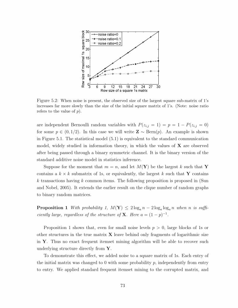
Figure 5.2: When noise is present, the observed size of the largest square sub-matrix of 1’sincreases far more slowly than the size of the initial square matrix of 1’s. (Note: noise ratiorefers to the value of p).

are independent Bernoulli random variables with P (zi,j = 1) = p = 1 − P (zi,j = 0)

for some p ∈ (0, 1/2). In this case we will write Z ∼ Bern(p). An example is shown

in Figure 5.1. The statistical model (5.1) is equivalent to the standard communication

model, widely studied in information theory, in which the values of X are observed

after being passed through a binary symmetric channel. It is the binary version of the

standard additive noise model in statistics inference.

Suppose for the moment that m = n, and let M(Y) be the largest k such that Y

contains a k × k submatrix of 1s, or equivalently, the largest k such that Y contains

k transactions having k common items. The following proposition is proposed in (Sun

and Nobel, 2005). It extends the earlier result on the clique number of random graphs

to binary random matrices.

Proposition 1 With probability 1, M(Y) ≤ 2 loga n − 2 loga loga n when n is suffi-

ciently large, regardless of the structure of X. Here a = (1− p)−1.

Proposition 1 shows that, even for small noise levels p > 0, large blocks of 1s or

other structures in the true matrix X leave behind only fragments of logarithmic size

in Y. Thus no exact frequent itemset mining algorithm will be able to recover such

underlying structure directly from Y.

To demonstrate this effect, we added noise to a square matrix of 1s. Each entry of

the initial matrix was changed to 0 with some probability p, independently from entry

to entry. We applied standard frequent itemset mining to the corrupted matrix, and

73

applied this process to matrices of different sizes. Figure 5.2 plots the size of the largest

recovered square sub-matrix of 1s against the size of the original matrix, for different

values of p (corresponding to different levels of data corruption). In the presence of

noise, only a fraction of the initial block of 1s was recovered, and this fraction diminished

with an increase in the size of the original matrix. Furthermore, the number of unique

itemsets reported increased exponentially with both corruption level and original block

size (see the spurious itemsets curve shown in Figure 5.9 in the experiment section).

The failure of classical frequent itemset mining to detect simple patterns in the

presence of random errors compromises the ability of these algorithms to detect as-

sociations, cluster items, or build classifiers when such errors are present. Noise is

ubiquitous in real data: it presents new challenges for algorithm development, and its

consequences should not ignored. In this paper, we focus on noise-tolerant frequent

itemset mining of the binary matrix representation of databases.

5.1.2 Approximate Frequent Itemset Models

The formal setting of our problem is as follows. The available data take the form of an

n×m binary matrixD. Each row ofD corresponds to a transaction i and each column of

D corresponds to an item j. The i, j-th element of D, denoted D(i, j), is 1 if transaction

i contains item j, and 0 otherwise. Let O = {i1, i2, . . . , in} and A = {j1, j2, . . . , jm}be the set of transactions and items associated with D, respectively. An itemset is

called frequent, if the fraction of transactions supporting it exceeds a given threshold,

minsup ∈ (0, 1].

One natural algorithmic approach for handling errors is to relax the requirement

that a sub-matrix determined by the frequent itemset consists entirely of 1s, and allow it

instead to contain a large fraction of 1s (and a small fraction of 0s), e.g., the “presence”

signal (Chakrabarti et al., 2004; Yang et al., 2001). This requirement is evidently a

necessary condition, but it is not sufficient to define a sub-matrix of interest. To see

why this is the case, consider the matrix shown in Figure 5.3.

The matrix in Figure 5.3 contains 3 sub-matrices {A,B,C}. The fraction of 1s

in each sub-matrix is the same, namely 75%, however, the 1s are distributed quite

differently in each. In sub-matrix A, each row and column contains 75% 1s, but in sub-

matrix B and C the 1s are concentrated in the dense sub-matrix B ∩C. Both column

g and row 7 are in a sense free riders on B ∩ C. Clearly, neither sub-matrix B nor

C should be used for association rule mining or classification purposes: in sub-matrix

74

11111111111

111111

11111111111

111111

A

B

C

a b c d e f g h

1

2

3

4

5

6

7

8

Figure 5.3: A binary matrix with three weak AFI(0.25) They can be more specifically clas-sified as, A: AFI(0.25, 0.25); B: AFI(*, 0.25); C: AFI(0.25, *).

B row 7 does not support any item in the itemset, and in sub-matrix C item g is not

supported by any transaction. It is possible to generate many more sub-matrices like

B and C by combining any of the remaining columns and rows with B ∩ C to form a

sub-matrices with densities of at least 75%.

Besides requiring a large fraction of 1s in a sub-matrix of interest, we advocate im-

posing two other conditions. First, for a given itemset, a supporting transaction should

contain most of the items. Second, to be included in an itemset, an associated item

has to appear in most of the supporting transactions. In the binary matrix representa-

tion, this means that the fraction of 0s in each row and each column of the sub-matrix

representing the approximate itemset has to fall below a user-defined threshold. The

threshold may differ for rows versus columns, and is denoted by εr and εc, respectively.

If the approximate itemset has sufficiently many rows, it is judged to be an approximate

frequent itemset (AFI).

Definition 5.1.1 Let D be as above, and let εr, εc ∈ [0, 1]. An itemset J ⊆ A is an

approximate frequent itemset AFI(εr, εc), if there exists a set of transactions I ⊆ O with

|I| ≥ |O| ·minsup such that the following two conditions hold:

1. ∀i ∈ I, 1

|J |∑j∈J

D(i, j) ≥ (1− εr);

2. ∀j ∈ J, 1

|I|∑i∈I

D(i, j) ≥ (1− εc);

Let AFI(εr, εc) denote the collection of all AFI sub-matrices of D. Classical or

75

exact frequent itemsets (EFI) are a special case of AFI, where both noise thresholds

εr and εc are set to zero. In cases where the noise in either the rows or the columns

is not restricted, AFI(εr, ∗) or AFI(∗, εc) is used to denote the corresponding families.

The noise threshold replaced by “∗” means that no constraint is employed for the

corresponding parameter, or the noise threshold is 1, i.e., ε = 1. We also define the

sub-matrices that satisfy the global noise constraint as weak AFIs in Definition 5.1.2.

Definition 5.1.2 Let D be as above, and let ε ∈ [0, 1]. An itemset J ⊆ A is a weak

AFI(ε) if there exists a set of transactions I ⊆ O with |I| ≥ |O| ·minsup such that the

following condition holds:

1

|I||J |∑i∈I

∑j∈J

D(i, j) ≥ 1− ε (5.2)

According to our definition, the three sub-matrices in Figure 5.3 are weak AFIs.

However, only sub-matrix A constitutes a valid AFI(0.25, 0.25). B and C do not satisfy

the constraints of AFI(0.25, 0.25), but they are valid AFI(∗, 0.25) and AFI(0.25, ∗)respectively.

Note that an AFI(εr, εc) also qualifies as both an AFI(εr, ∗) and an AFI(∗, εc).The relationships among the various criteria are summarized in the Venn diagram of

Figure 5.4. The differences in the sizes of the families and the maximum lengths of

itemsets contained in each leads to substantial differences in the computational costs

for the algorithms that search for them. This will be further elaborated upon in the

experimental sections.

In this work we proceed from the premise that, while the exact frequent itemset

criterion is too restrictive, simple application of the weak AFI, AFI(εr, ∗) and AFI(∗, εc)criteria allows poor approximations to frequent itemsets.

Yang et.al. (Yang et al., 2001) have developed models equivalent to the weak AFI

and AFI(εr, ∗), but use the terms weak ETI and strong ETI, respectively, instead. For

ease in comparing the competing criteria, we adopt their terminology for the remainder

of this paper.

5.1.3 Challenges and Contributions

Accommodating the refined noise criteria creates substantial algorithmic challenges not

posed by exact frequent itemset mining. First and foremost, the AFI criterion distin-

76

Figure 5.4: Relationships of various AFI criteria.

guishes itself from traditional exact frequent itemsets as it violates the anti-monotone

(Apriori) property. An exact itemset cannot be frequent if any of its sub-itemsets fails

to be frequent. However, a sub-itemset of an AFI need not be an AFI. For example,

given minsup = 4 and εr = εc = 25%, sub-matrix A in Figure 5.3 is a valid AFI, but

none of its sub-itemsets have sufficient support to be an AFI. Theminsup can no longer

be employed as a pruning threshold for itemset. No accurate pruning threshold has

ever been found in any of existing work on noise-tolerant itemset mining. As a result,

algorithms, such as ETI mining, have to rely on heuristics to prune the search space.

These heuristics do not guarantee the completeness of the search. Another algorithm

to discover dense itemsets (Sepp and Mannila, 2004) enforces the constraint that all

sub-itemsets of a dense itemset must be frequent. Since this algorithm requires minsup

support for all sub-itemsets, it can fail to identify larger itemsets that have sufficient

support.

Noise-tolerance also affects the way in which supporting transactions are maintained

in the algorithm. With exact frequent itemset mining, a transaction supporting an

itemset also supports its sub-itemsets. This property is fundamental to any depth-

first approach. This property, however, does not hold for AFI: one cannot derive the

support set of an AFI from the common support sets of its sub-patterns, as is done in

exact frequent itemset mining. (Examination of sub-matrix A in Figure 5.3 makes this

clear.) To solve this problem, the algorithms proposed in(Yang et al., 2001; Sepp and

Mannila, 2004) require repeated scans of the entire database to identify the support for

each itemset. The exponential number of potential itemsets makes this very expensive.

In this paper, we investigate the noise-tolerant property of approximate frequent

itemsets that provides both the algorithmic basis for itemset generation, and the po-

77

tential for pruning based on an AFI’s support. The property is a generalization of

Apriori under noisy conditions and includes the Apriori property as a special case when

noise is absent. By incorporating noise-tolerant attributes, we designed an efficient and

effective approach for mining the complete set of approximate frequent itemsets.

5.1.4 Outline

The rest of the chapter is organized as follows. Section 5.2 outlines related work in

the area of noise-tolerant itemset mining. Section 5.3 contains a theoretical analysis

showing how the AFI criterion can be used to recover block structures in the presence of

noise, a problem for which standard frequent pattern mining fails. Section 5.4 presents

the algorithm and two pruning strategies. Assessment of the AFI algorithm on synthetic

and real data sets and an examination of its scalability are presented in Section 5.5.

Section 5.6 concludes the paper.

5.2 Background and Related Work

In the standard frequent itemset problem (Agrawal and Srikant, 1995), the goal is

to enumerate all the frequent itemsets in D; there is no allowance for noise. This

corresponds to our AFI definition when εr = εc = 0.

Noise-tolerant itemsets were first discussed by in (Yang et al., 2001), who proposed

two error tolerant models, termed weak error-tolerant itemsets (ETI)(equivalent to

weak AFI) and strong ETI (equivalent to AFI(ε, ∗)). As noted in the discussion of

Figure 5.3, the ETI models do not preclude columns of zeros. Although this problem is

identified by Yang et al. (Yang et al., 2001), it is not resolved in their paper. In addition,

without an efficient pruning technique the authors had to employ a variety of heuristics

and sampling techniques instead. In (Sepp and Mannila, 2004) the authors seek weak

ETIs by constraining the subsets of ETIs to also be weak ETIs. This constraint may

not only miss valid itemsets of interest, but also generates irrelevant itemsets, such as

cluster (B) in Figure 5.3.

Other lines of work to find itemsets tolerating noise are (Steinbach et al., 2004).

These approaches admit only a fixed number of 0s in the itemsets. In contrast to our

AFI model, the fraction of noise can not vary with the size of a submatrix defining

an itemset, and therefore, is not guaranteed to be bounded relative to the size of the

result. The support envelope technique (Steinbach et al., 2004) identifies regions of the

78

data matrix where each transaction contains at least a given number of items and each

item appears in at least a given number of transactions. The support envelope is a

tool for exploring and visualizing high-level itemset structures in a data matrix. The

paper defines a symmetric error tolerant itemset model (Symmetric ETI). It is similar

to AFI but restricts the fraction of errors allowed to be the same for columns and rows.

Also, no additional properties or algorithms for the symmetric ETI are developed by

the authors.

5.3 Recovery of Block Structures in Noise

In this section we present some theoretical support for the AFI model in the context

of a simple recovery problem for matrices with noise. Proposition 1 of Section 5.1.1

shows that exact frequent itemset mining cannot directly recover blocks of 1s and other

structures in the presence of noise. The weak ETI (weak AFI), ETI (AFI(εr, *)) and

AFI model address this problem by allowing zeros in their target sub-matrices. One

means of validating and comparing these criteria is to see if they are able to recover

simple structures in cases where exact frequent pattern mining fails. To this end, we

show how the AFI model can be applied to the simple problem of recovering a sub-

matrix of 1s set against a background of zeros when noise is present. (A complete

analysis can be found in (Sun and Nobel, 2005)). For simplicity, we only consider

square matrices and sub-matrices. However, analogous results hold for rectangular

matrices and sub-matrices.

Let X be an n × n binary matrix that consists of an l × l sub-matrix C∗ of 1s,

with all other entries equal to 0. (Note that the rows and columns of C∗ need not

be contiguous.) Suppose that we observe Y = X ⊕ Z, where Z ∼ Bern(p), with

0 < p < 1/2, and wish to accurately recover C∗. Let p0 be any number such that

p < p0 < 1/2, and let τ = 1− p0 be an associated error threshold. If C is a sub-matrix

of X, let C ∈ AFIτ (X) denote the fact that every row and column of C has at least

100 τ% 1s.

In order to recover C∗, we identify the largest square AFI in the observed matrix

Y having an error threshold τ . More precisely, let C be the family of all square sub-

matrices C of X such that C ∈ AFIτ (X), and define

C = argmaxC∈C|C|

79

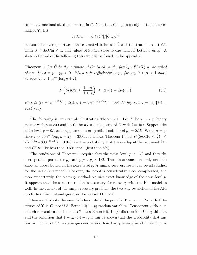
to be any maximal sized sub-matrix in C. Note that C depends only on the observed

matrix Y. Let

SetClu = |C ∩ C∗|/|C ∪ C∗|

measure the overlap between the estimated index set C and the true index set C∗.

Then 0 ≤ SetClu ≤ 1, and values of SetClu close to one indicate better overlap. A

sketch of proof of the following theorem can be found in the appendix.

Theorem 1 Let C be the estimate of C∗ based on the family AFIτ (X) as described

above. Let δ = p − p0 > 0. When n is sufficiently large, for any 0 < α < 1 and l

satisfying l > 16α−1(logb n+ 2),

P

(SetClu ≤ 1− α

1 + α

)≤ ∆1(l) + ∆2(α, l). (5.3)

Here ∆1(l) = 2e−3 δ2 l/8p, ∆2(α, l) = 2n−14αl+4 logb n, and the log base b = exp{3(1 −

2 p0)2/8p}.

The following is an example illustrating Theorem 1. Let X be a n × n binary

matrix with n = 800 and let C∗ be a l × l submatrix of X with l = 400. Suppose the

noise level p = 0.1 and suppose the user specified noise level p0 = 0.15. When α = 14,

since l > 16α−1(logb n + 2) = 360.1, it follows Theorem 1 that P(SetClu ≤ 3

5

)≤

2(e−3.75 +800−10.448) = 0.047, i.e. the probability that the overlap of the recovered AFI

and C* will be less than 0.6 is small (less than 5%).

The conditions of Theorem 1 require that the noise level p < 1/2 and that the

user-specified parameter p0 satisfy p < p0 < 1/2. Thus, in advance, one only needs to

know an upper bound on the noise level p. A similar recovery result can be established

for the weak ETI model. However, the proof is considerably more complicated, and

more importantly, the recovery method requires exact knowledge of the noise level p.

It appears that the same restriction is necessary for recovery with the ETI model as

well. In the context of the simple recovery problem, the two-way restriction of the AFI

model has direct advantages over the weak-ETI model.

Here we illustrate the essential ideas behind the proof of Theorem 1. Note that the

entries of Y in C∗ are i.i.d. Bernoulli(1− p) random variables. Consequently, the sum

of each row and each column of C∗ has a Binomial(l,1−p) distribution. Using this fact

and the condition that 1 − p0 < 1 − p, it can be shown that the probability that any

row or column of C∗ has average density less than 1 − p0 is very small. This implies

80

that C∗ ∈AFIτ (X) with high probability. Since C is the maximal sized sub-matrix in

AFIτ (X), it follows that |C| is greater than or equal to |C∗| with high probability. Now,

we want to show that C can not be too large either, and that it can only contain a small

proportion of entries outside C∗. When C is much larger than C∗, it must contain a

large number of rows (or columns) whose entries are from outside C∗. The definition of

C via the AFI criterion implies that each such row (column) has density greater than

τ . Moreover, the rows (columns) will necessarily contain a large rectangular region

with entries from outside C∗, and this region should also have density greater than τ .

But as the entries of Y outside C∗ are i.i.d. Bernoulli(p), the probability of finding a

rectangular region as above is very small.

Theorem 1 can readily be applied to the asymptotic recovery of structure in a

sequential framework. Suppose that {Xn : n ≥ 1} is a sequence of square binary

matrices, where Xn is n × n and consists of an ln × ln sub-matrix C∗n of 1s with all

other entries equal to 0. For each n we observe Yn = Xn ⊕ Zn, where Zn ∼Bern(p),

and wish to recover C∗n. Let SetClun measure the overlap between C∗

n and the estimate

Cn produced by the AFI recovery method above. The following corollary of Theorem

1 shows that, under suitable conditions on ln, Cn provides asymptotically consistent

estimates of C∗n. The proof can be found in the appendix.

Corollary 1 If ln > 16ψ(n)(logb n + 2) where ψ(n) → ∞ as n → ∞, then with

probability one

SetClun ≤1− ψ(n)−1

1 + ψ(n)−1

when n is sufficiently large.

5.4 AFI Mining Algorithm

Mining approximate frequent itemsets poses a number of new algorithmic challenges

beyond those faced when mining exact itemsets. The foremost difficulty is that noise-

tolerant itemset mining cannot employ the anti-monotone property that has led to

the success of frequent itemset mining. The development of an efficient algorithm for

finding AFIs calls for new itemset generation strategies to limit the search space. We

present a noise-tolerant Apriori property in Section 5.4.1. In addition, the AFI criteria

allow the number of errors to increase with the size of the itemset. It is therefore critical

to take account of the additional errors in an itemset as its dimensionality increases

while collecting the supporting transactions. Solving this problem is the key to AFI

81

mining, and is addressed in subsection 5.4.1. The AFI mining algorithm adapts the

methods of level-wise breadth-first frequent itemset mining to this new setting, and

takes advantage of our new techniques to generate noise-tolerant approximate frequent

itemsets.

5.4.1 Mining AFIs

The algorithm’s enumeration of the AFI differs from the existing work of weak ETI

algorithm(Yang et al., 2001) in the following aspects: First, even though the Apriori

property doesn’t hold for any type of AFI(except those that allow no noise), we have

developed a noise-tolerant Apriori property (Theorem 5.4.1) and apply it to prune and

generate candidate itemsets. Secondly, by taking different approaches in extending the

itemsets, we are able to collect the support of an noise-tolerant itemset based on the

support set in the sub-itemsets.

Noise-Tolerant Support Pruning

The anti-monotone property of exact frequent itemsets is the key to minimizing expo-

nential searches in frequent itemset mining. In particular, the anti-monotone property

ensures that a (k + 1) exact itemset can be pruned if any one of its k sub-itemsets is

not frequent. However, this property is no longer true for any variation of AFI. In-

stead, in this paper, we derive a noise-tolerant support to serve as the Apriori pruning

threshold. The noise-tolerant support is determined by the size of the itemset and the

noise thresholds. This support threshold leads to substantial performance gain for our

algorithm.

Theorem 5.4.1 Given a support threshold minsup, if a length (k + 1)-itemset J ′ is

an AFI(εr, εc), then for any of its k item subset J ⊆ J ′, the number of transactions

containing no more than εr fraction of noise in J is at least

n ·minsup ·(− kεcbkεrc+ 1

)(5.4)

Proof: By assumption, there exists a set of transactions I ′ such that |I ′| ≥ n ·minsupand I ′ × J ′ ∈ AFI(εr, εc) Let J be a k item subset of J ′ with support set I. Thus each

i ∈ I contains at most kεr zeros on J .

82

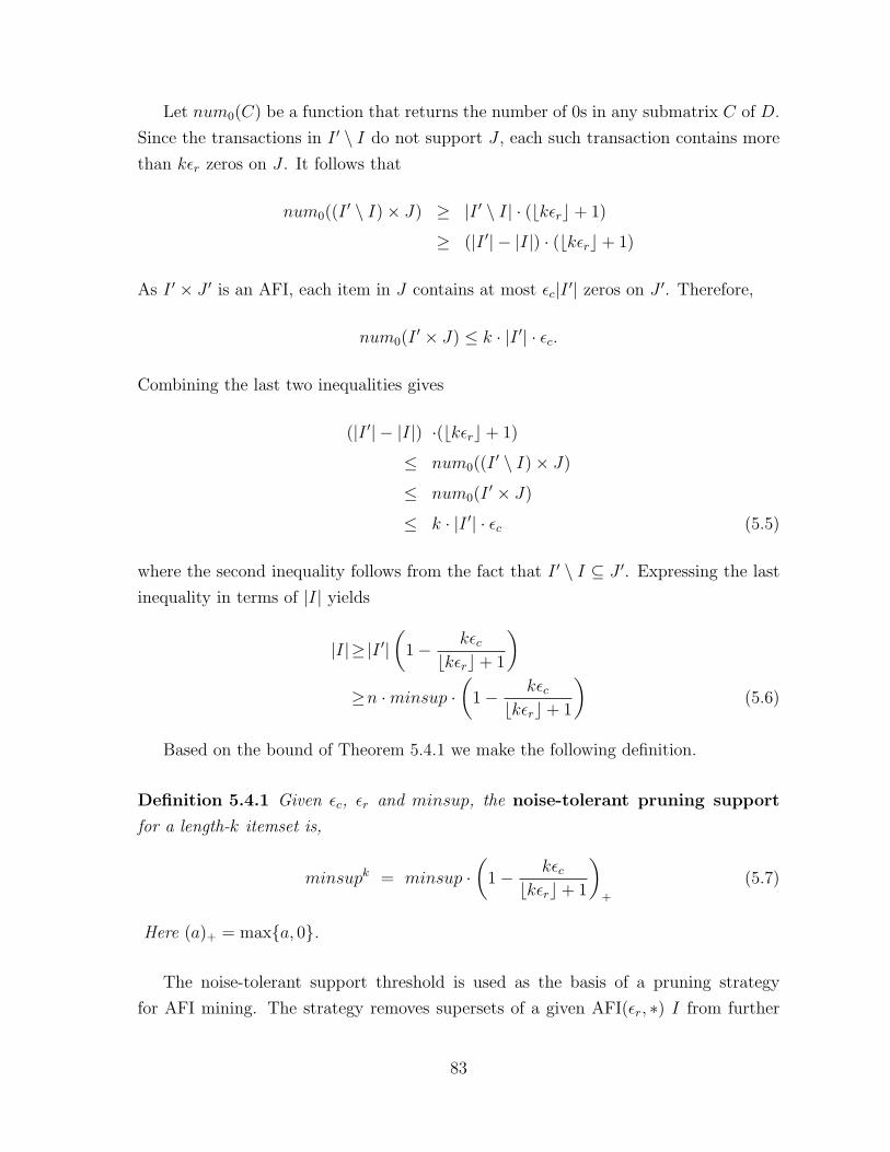
Let num0(C) be a function that returns the number of 0s in any submatrix C of D.

Since the transactions in I ′ \ I do not support J , each such transaction contains more

than kεr zeros on J . It follows that

num0((I′ \ I)× J) ≥ |I ′ \ I| · (bkεrc+ 1)

≥ (|I ′| − |I|) · (bkεrc+ 1)

As I ′ × J ′ is an AFI, each item in J contains at most εc|I ′| zeros on J ′. Therefore,

num0(I′ × J) ≤ k · |I ′| · εc.

Combining the last two inequalities gives

(|I ′| − |I|) ·(bkεrc+ 1)

≤ num0((I′ \ I)× J)

≤ num0(I′ × J)

≤ k · |I ′| · εc (5.5)

where the second inequality follows from the fact that I ′ \ I ⊆ J ′. Expressing the last

inequality in terms of |I| yields

|I|≥ |I ′|(

1− kεcbkεrc+ 1

)≥n ·minsup ·

(1− kεcbkεrc+ 1

)(5.6)

Based on the bound of Theorem 5.4.1 we make the following definition.

Definition 5.4.1 Given εc, εr and minsup, the noise-tolerant pruning support

for a length-k itemset is,

minsupk = minsup ·(

1− kεcbkεrc+ 1

)+

(5.7)

Here (a)+ = max{a, 0}.

The noise-tolerant support threshold is used as the basis of a pruning strategy

for AFI mining. The strategy removes supersets of a given AFI(εr, ∗) I from further

83

consideration when the number of transactions which contain less than εr fraction of

errors in I is less than n ·minsupk. In the special case that εr = εc = 0, minsupk =

minsup, which is consistent with the anti-monotone property of exact frequent itemsets.

The support threshold decreases as εc increases and as εr decreases. In the former case,

a less stringent column constraint is applied to a block with fixed row constraints, and

conversely in the case of decreasing εr. In particular, the support threshold is equal to

0 when k · εc > dk · εre. Therefore, no pruning can be applied at all.

0/1 Extensions

Starting with singleton itemsets, the AFI algorithm generates (k + 1)-itemsets from

k-itemsets in a sequential fashion. The number of 0s allowed in the itemset grows with

the length of the itemset in a discrete manner. If b(k+1)εrc > bkεrc, then transactions

supporting the (k+1)-itemset are permitted one more zero than transactions supporting

k-itemsets. When b(k + 1)εrc = bkεrc, no additional zeros are allowed. For example,

if εr = 0.25, additional zeros are permitted in transactions when extending itemsets of

length 3, 7, 11 and so on. Whether the maximal number of zeros will increase in a (k+1)

itemset makes a difference in deriving its set of supporting transactions. Intuitively, if

an additional zero is allowed at level (k + 1), any transaction supporting a k itemset

should also support its (k+1) superset. On the other hand, when the maximum number

of zeros allowed in an itemset stay the same at level (k + 1), a transaction that does

not support k itemset will not have enough 1s to support its (k + 1) superset. These

two properties are formally addressed in Lemma 5.4.2 and Lemma 5.4.3 as 1-Extension

and 0-Extension respectively.

Lemma 5.4.2 (1-Extension) If bk · εrc = b(k + 1) · εrc then any transaction that does

not support a k-itemset will not support its (k + 1) item superset.

The Lemma is based on the fact that if no additional noise is allowed when generat-

ing a (k + 1) itemset, a transaction that does not support a k-itemset will not support

its (k + 1) superset since the number of 1s it contains is always smaller than or equal

or bk∗εc−1+1k+1

< ε. Thus if bk · εrc = b(k + 1) · εrc then the transaction set of a (k + 1)

itemset I is the intersection of the transaction sets of its length k subsets. This is called

a 1-extension.

Lemma 5.4.3 (0-Extension) If bk·εrc+1 = b(k+1)·εrc then any transaction supporting

a k-itemset also supports its (k+1) supersets.

84

The procedure of 0-extension illustrates how noise can be incorporated into a fre-

quent itemset. If additional noise is allowed for a (k+1) itemset relative to a k itemset,

it is intuitive that a transaction that supports a k-itemset will also support its (k+ 1)-

item supersets, no matter whether the (k+1)th entry is 1 or 0. To utilize this property,

if bk · εrc+ 1 = b(k + 1) · εrc, the transaction set of a (k + 1) itemset I is the union of

the transaction sets of its length k subsets. This is called a 0-extension.

8:Φ

ab ad cdbc bdac

abd acd bcdabc

abcd

b c dT:{1,2,3,5,8}

aT:{1,2,4,5,7} T:{1,3,4,5} T:{5,6,7}

* a b c1 1 1 12 1 1 03 1 0 14 0 1 15 1 1 1

b c d1 1 1 04 1 1 05 1 1 17 1 0 1

a b c d1 1 1 1 05 1 1 1 1

a b d1 1 1 02 1 1 05 1 1 17 0 1 1

a c d1 1 1 03 1 1 05 1 1 1

Level:0

Level:1

Level:2

Level:3

Level:4

a b1 1 12 1 15 1 1

a c1 1 13 1 15 1 1

a d5 1 1

b d5 1 17 1 1

c d5 1 1

1-extension

1-extension

0-extension

1-extension

b c1 1 14 1 15 1 1

a b c d1 1 1 1 02 1 1 0 03 1 0 1 04 0 1 1 05 1 1 1 16 0 0 0 17 0 1 0 18 1 0 0 0

(A) (B)

Figure 5.5: (A) Sample database; (B) Level wise mining of AFI in database (A). SeeSection 5.4.2 for more details. Only black colored itemsets will be generated by AFI, whileevery itemset including the grey-colored itemsets will have to be generated to mine ETIs.

0-extension and 1-extension suggest two basic steps to be taken for efficient mainte-

nance of the supporting transactions. They allow the algorithm to obtain the support

transactions of an itemset from its item subsets while avoiding the repeated scan of

databases that plagues the algorithms proposed by (Yang et al., 2001; Sepp and Man-

nila, 2004). In the next section, we illustrate through an example the use of the two

techniques together with noise-tolerant support-based pruning method.

5.4.2 An Example

In this section we present a simple example in which the data matrix D of Figure 5.5

is used to illustrate the AFI algorithm. Let εr = εc = 1/3 and let minsup = 0.5. The

number of transactions in the database, n, equals 8. We wish to find the complete set

of AFIs in D. In this case, the algorithm proceeds as follows.

85

Step 1: k = 1,minsup1 = 0.5. The database is scanned once and the support of

each singleton item is recorded.

Step 2: k = 2,minsup2 = 0.5∗1/3. As bk · εrc = b(k−1) · εrc, no additional 0’s are

allowed and a 1-extension is performed. In particular, the transaction set of the itemset

ab is obtained by intersecting the transaction set of a, equal to {1, 2, 3, 5, 8}, with that

of b, equal to {1, 2, 4, 5, 7}; the result is {1, 2, 5}. Since the number of transactions

supporting ad and cd is equal to 1. Therefore, their supports are below the support

threshold minsup2, any AFI that contains them can be pruned. These itemsets are

colored gray in Figure 5.5.

Step 3: k = 3,minsup3 = 0.5 ∗ 2/3. In this case, bk · εrc = b(k − 1) · εr)c + 1.

Thus one additional 0 is allowed in 3-itemsets, and a 0-extension (union of transaction

sets) is performed. For example, a transaction supports itemset abc if it supports any of

{ab, ac, bc}; the transaction set of abc is the union of the transaction sets for {ab, ac, bc},which is {1, 2, 5} ∪ {1, 3, 5} ∪ {1, 4, 5} = {1, 2, 3, 4, 5}.

Step 4: k = 4,minsup4 = 0.5 ∗ 1/3. Because of support constraint minsup, i.e,

0.5, {a, b, c, d} cannot be a valid AFI. No further extension of the current itemset is

possible since all of the search space is covered.

Step 5: The candidate AFIs are {b, d} and {a, b, c}. The first does not satisfy the

minsup size constraint. The second is readily shown to be a valid AFI, and constitutes

the output of the algorithm.

5.4.3 Global Pruning

In order for an individual item i to appear in an AFI, its overall support must exceed

minsup ·n · (1− εc). During the level-wise generation of AFI(εr, ∗), the total number of

transactions under consideration in a given level will decrease or remain the same, and

the number of transactions supporting an individual item will have the same property. If

the support of item i among the transactions at level k drops below minsup ·n · (1−εc),then i can not appear in any AFI generated at levels k′ ≥ k. In particular, any

itemset containing i can be eliminated from consideration. To illustrate, in the example

presented in Figure 5.5 the number of transactions supporting an itemset should not

be below 4. In addition, the number of supporting transactions for an individual item

has to be above d4 · (1 − εc)e = d4(1 − 1/3)e = 3. The set of transactions remaining

at level 2 is T = {1, 2, 3, 5, 7}; the number of transactions in T supporting item d is 2,

which is less than 3, so any itemset in level k ≥ 2 containing d can be eliminated from

86

Algorithm 6 AFI MiningInput: D, εr, εc, minsupOutput: The sets of approximate frequent itemsets

for i = 1 : m doT(i)=genSupport(D, i);

end fork = 1;L1=∪m

i>0{i};repeat

k := k+1;Lk := GenCandidateItemset(Lk−1,minsup

k−1)if (bk · εrc = b(k + 1) ∗ εrc) then

T(Lk) := 1-Extension(I,Lk−1);else

T(Lk) := 0-Extension(I,Lk−1);end ifAFIp := AFIp ∪ Lk;

until Lk is ∅AFI :=filter(AFIp,minsup, εc)return AFI

consideration.

5.4.4 Identification of AFI

The AFI algorithm so far generates a superset of approximate frequent itemsets. The

postprocessing of this subset can be done separately from the level-wise generation since

it will neither benefit nor prohibit the traversing of the search space. The verification of

whether an AFI(εr, ∗) is an AFI can be easily done by simply checking the percentage

of 0’s in each candidate itemset. Finding a maximal AFI in an AFI(εr, ∗) is more

difficult. In (Liu et al., 2005), we describe a heuristic algorithm for this problem that

scales linearly with respect to |T |+|I|, where I is an itemset supported by a transaction

set T . The algorithm works by removing transactions having a large number of zeros,

beginning with those whose zeros are aligned with low density items. Due to space

limitations, a complete description of this algorithm is omitted.

87

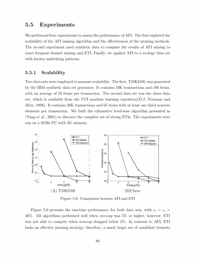
5.5 Experiments

We performed four experiments to assess the performance of AFI. The first explored the

scalability of the AFI mining algorithm and the effectiveness of the pruning methods.

The second experiment used synthetic data to compare the results of AFI mining to

exact frequent itemset mining and ETI. Finally, we applied AFI to a zoology data set

with known underlying patterns.

5.5.1 Scalability

Two data sets were employed to measure scalability. The first, T10KI100, was generated

by the IBM synthetic data set generator. It contains 10K transactions and 100 items,

with an average of 10 items per transaction. The second data set was the chess data

set, which is available from the UCI machine learning repository(D.J. Newman and

Merz, 1998). It contains 28K transactions and 65 items with at least one third nonzero

elements per transaction. We built the exhaustive level-wise algorithm presented in

(Yang et al., 2001) to discover the complete set of strong ETIs. The experiments were

run on a 2GHz PC with 2G memory.

(A) T10KI100 (B)Chess

Figure 5.6: Comparison between AFI and ETI

Figure 5.6 presents the run-time performance for both data sets, with εr = εc =

20%. All algorithms performed well when minsup was 5% or higher; however, ETI

was not able to compete when minsup dropped below 2%. In contrast to AFI, ETI

lacks an effective pruning strategy; therefore, a much larger set of candidate itemsets

88

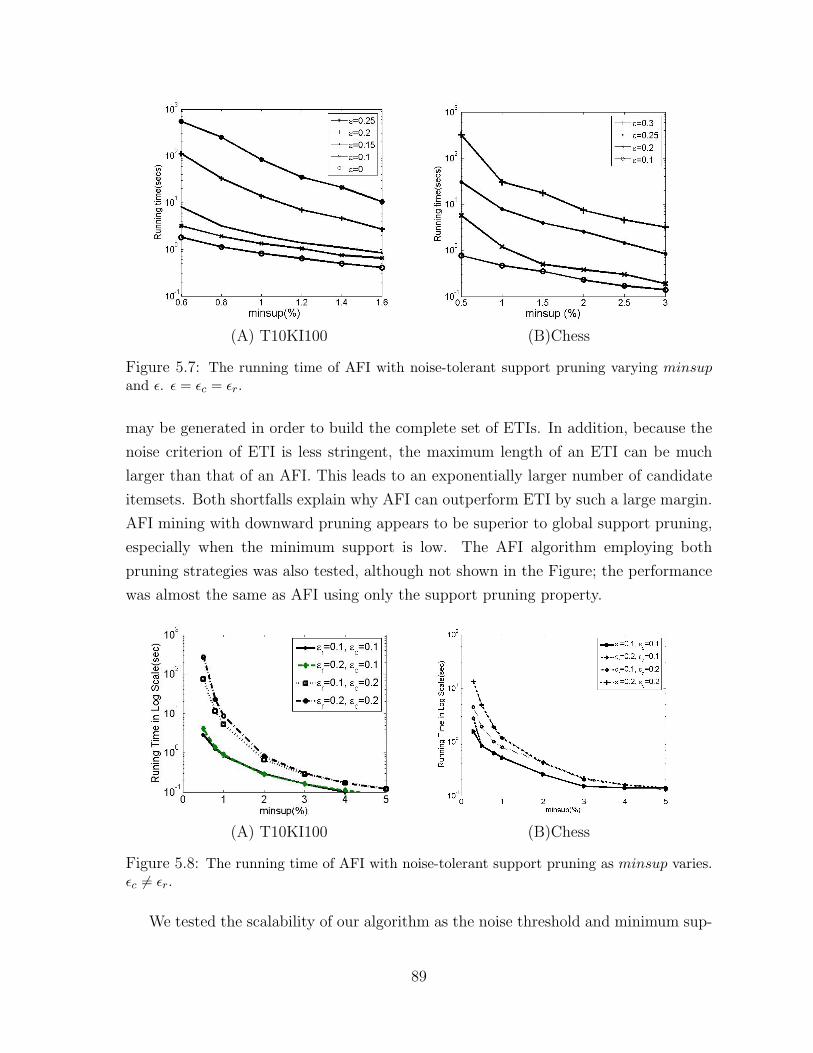
(A) T10KI100 (B)Chess

Figure 5.7: The running time of AFI with noise-tolerant support pruning varying minsupand ε. ε = εc = εr.

may be generated in order to build the complete set of ETIs. In addition, because the

noise criterion of ETI is less stringent, the maximum length of an ETI can be much

larger than that of an AFI. This leads to an exponentially larger number of candidate

itemsets. Both shortfalls explain why AFI can outperform ETI by such a large margin.

AFI mining with downward pruning appears to be superior to global support pruning,

especially when the minimum support is low. The AFI algorithm employing both

pruning strategies was also tested, although not shown in the Figure; the performance

was almost the same as AFI using only the support pruning property.

(A) T10KI100 (B)Chess

Figure 5.8: The running time of AFI with noise-tolerant support pruning as minsup varies.εc 6= εr.

We tested the scalability of our algorithm as the noise threshold and minimum sup-

89

port varied. The result is shown in Figure 5.7. To reduce the parameter space, the

transaction-wise threshold εr was set equal to the item-wise noise threshold εc in this

set of experiments. Figure 5.7 shows that running time increases with increases in noise

tolerance, as expected. Here the algorithm is essentially looking for approximate fre-

quent itemsets with higher-dimensionality. Allowing more noise in an itemset results in

larger approximate frequent itemsets; consequently, more candidate itemsets have to be

explored, and computation increases exponentially with respect to the dimensionality

of the itemsets. Nevertheless, even with a very high error rate of 30%, our algorithm

proves competent in finding the complete sets of AFI in a reasonable time.

Figure 5.8 shows how different transaction-wise and item-wise noise thresholds can

affect performance. Relatively speaking, reducing the item-wise error constraint leads to

a greater reduction in running time than reducing the transaction-wise error constraint,

as the former leads to higher levels of pruning according to Theorem 5.4.1.

5.5.2 Quality Testing with Synthetic Data

In addition to run-time performance we also tested the quality of the results produced

by AFI. To do so we created data with an embedded pattern and then overlaid random

errors. By knowing the true patterns, we were able to assess the quality of the various

results. To each synthetic data set created, an exact method (ETI with εc = 0), ETI

and AFI were each applied.

To evaluate the performance of an algorithm on a given data set, we employed two

measures that jointly describe quality: “recoverability” and “spuriousness.” Recov-

erability is the fraction of the embedded patterns recovered by an algorithm, while

spuriousness is the fraction of the mined results that fail to correspond to any planted

cluster. A truly useful data mining algorithm should achieve high recoverability with

little spuriousness to dilute the results. A detailed description of the two measures is

given in (Liu et al., 2005). Multiple data sets were created and analyzed to explore

the relationship between increasing noise levels and the quality of the result. Noise

was introduced by bit-flipping each entry of the full matrix with a probability equal

to p. The probability p was varied over different runs from 0.01 to 0.2. The number

of pattern blocks embedded also varied, but the results were consistent across this pa-

rameter. Here we present results when 1 or 3 blocks were embedded in the data matrix

(Figure 5.9(A) and (B), respectively).

In both cases, the exact method performed poorly as noise increased. Beyond p =

90

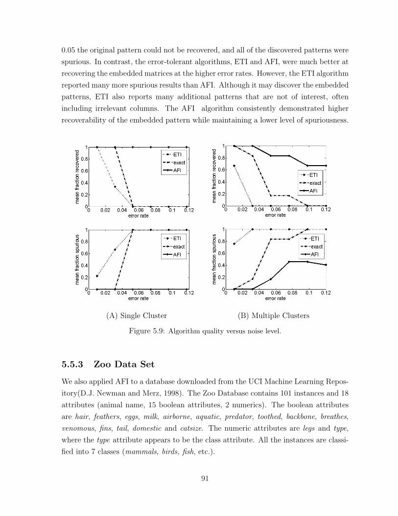
0.05 the original pattern could not be recovered, and all of the discovered patterns were

spurious. In contrast, the error-tolerant algorithms, ETI and AFI, were much better at

recovering the embedded matrices at the higher error rates. However, the ETI algorithm

reported many more spurious results than AFI. Although it may discover the embedded

patterns, ETI also reports many additional patterns that are not of interest, often

including irrelevant columns. The AFI algorithm consistently demonstrated higher

recoverability of the embedded pattern while maintaining a lower level of spuriousness.

(A) Single Cluster (B) Multiple Clusters

Figure 5.9: Algorithm quality versus noise level.

5.5.3 Zoo Data Set

We also applied AFI to a database downloaded from the UCI Machine Learning Repos-

itory(D.J. Newman and Merz, 1998). The Zoo Database contains 101 instances and 18

attributes (animal name, 15 boolean attributes, 2 numerics). The boolean attributes

are hair, feathers, eggs, milk, airborne, aquatic, predator, toothed, backbone, breathes,

venomous, fins, tail, domestic and catsize. The numeric attributes are legs and type,

where the type attribute appears to be the class attribute. All the instances are classi-

fied into 7 classes (mammals, birds, fish, etc.).

91

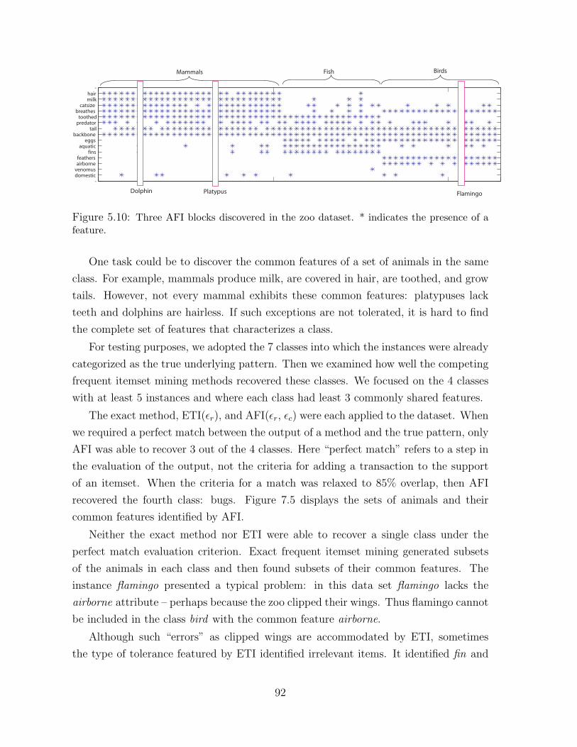
-hairmilk

catsizebreathes

toothedpredator

tailbackbone

eggsaquatic

finsfeathersairborne

venomusdomestic

-

Fish Birds

FlamingoDolphin Platypus

Mammals

Figure 5.10: Three AFI blocks discovered in the zoo dataset. * indicates the presence of afeature.

One task could be to discover the common features of a set of animals in the same

class. For example, mammals produce milk, are covered in hair, are toothed, and grow

tails. However, not every mammal exhibits these common features: platypuses lack

teeth and dolphins are hairless. If such exceptions are not tolerated, it is hard to find

the complete set of features that characterizes a class.

For testing purposes, we adopted the 7 classes into which the instances were already

categorized as the true underlying pattern. Then we examined how well the competing

frequent itemset mining methods recovered these classes. We focused on the 4 classes

with at least 5 instances and where each class had least 3 commonly shared features.

The exact method, ETI(εr), and AFI(εr, εc) were each applied to the dataset. When

we required a perfect match between the output of a method and the true pattern, only

AFI was able to recover 3 out of the 4 classes. Here “perfect match” refers to a step in

the evaluation of the output, not the criteria for adding a transaction to the support

of an itemset. When the criteria for a match was relaxed to 85% overlap, then AFI

recovered the fourth class: bugs. Figure 7.5 displays the sets of animals and their

common features identified by AFI.

Neither the exact method nor ETI were able to recover a single class under the

perfect match evaluation criterion. Exact frequent itemset mining generated subsets

of the animals in each class and then found subsets of their common features. The

instance flamingo presented a typical problem: in this data set flamingo lacks the

airborne attribute – perhaps because the zoo clipped their wings. Thus flamingo cannot

be included in the class bird with the common feature airborne.

Although such “errors” as clipped wings are accommodated by ETI, sometimes

the type of tolerance featured by ETI identified irrelevant items. It identified fin and

92

domestic as common features for mammals, which is not generally true. Because only

the row-wise constraint was applied, the set of features discovered was not reliable.

5.6 Conclusion

In this chapter we have outlined an algorithm for mining approximate frequent itemsets

from noisy data. The AFI model places two criteria on the fraction of noise in both

the rows and columns, and so ensures a relatively reasonable distribution of the error

in any patterns found. Our work generalizes the classical level-wise frequent itemset

mining based on the Apriori-property into a new algorithm where the Apriori-property

does not hold and noise has to be incorporated. Our work generates not only more

reasonable and useful itemsets than classical frequent itemset mining and existing noise-

tolerant frequent itemset mining, but it is computationally more efficient as well. We are

currently investigating depth-first methods for approximate frequent itemset mining.

5.7 Appendix

The detailed proofs of the following Lemma 1 and Lemma 2 can be found in (Sun and

Nobel, 2005). We only state them here.

Lemma 1 Under the conditions of Theorem 1,

P(|C| ≤ l2

)≤ ∆1(l). (5.8)

Lemma 2 For any sufficiently large n, let A = {C : C ∈ Cn such that |C| > l2

2and |C∩C∗c|

|C| ≥α}. Let A = {A 6= ∅}. If l ≥ 16α−1(logb n+ 2), then

P (A) ≤ ∆2(α, l)

Proof of Theorem 1: Let E be the event that {SetClu ≤ 1−α1+α}. It is clear that E

can be expressed as the union of two disjoint events E1 and E2, where

E1 = {|C| ≤ |C∗|} ∩ E

and

E2 = {|C| > |C∗|} ∩ E

93

On the other hand, by the definition of SetClu, inequality SetClu ≤ 1−α1+α

can be rewrit-

ten equivalently as

1 +|C ∩ C∗c||C ∩ C∗|

+|Cc ∩ C∗||C ∩ C∗|

≥ 1 + α

1− α.

Moreover, when |C| > |C∗|, one can verified the trivial fact that |C ∩C∗c| > |Cc ∩C∗|,which also implies that

1 +|C ∩ C∗c||C ∩ C∗|

+|Cc ∩ C∗||C ∩ C|

≤ 1 + 2|C ∩ C∗c||C ∩ C∗|

.

Furthermore, one can verified that E2 ⊂ E ′2, where

E ′2 = {|C| > |C∗|} ∩

{1 + 2

|C ∩ C∗||C ∩ C∗|

≥ 1 + α

1− α

}.

Therefore, it suffices to bound P (E) by P (E1) and P (E ′2) separately.

Immediately, one can bound P (E1) by ∆1(l) via Lemma 1. It remains to bound

P (E ′2). Notice that inequality

1 + 2|C ∩ C∗c||C ∩ C∗|

≥ 1 + α

1− αimplies

|C ∩ C∗c||C|

≥ α.

Therefore, by Lemma 2, one can bound P (E ′2) by

P (E ′2) ≤ P

(E ′

2

∣∣∣|C| ≥ l2)≤ ∆2(α, l),

where the first inequality holds because the unconditional probability is always less or

equal to the conditional probability. Consequently, we have

P

(SetClu ≤ 1− α

1 + α

)≤ ∆1(l) + ∆2(α, l).

Proof of Corollary 1: Theorem 1 implies that if we can bound both ∆1(ln) and

∆2(ψ(n)−1, ln) by 2n−2 for any sufficiently large n, then Borel -Cantelli Lemma can be

applied to establish the almost sure convergency.

When n is sufficiently large, the condition ln > 16ψ(n)(logb n + 2) and ψ(n) → n,

implies ln > 2(34(p − p0)

2 logb e)−1 logb n. By plugging this lower bound of ln into

∆1(ln), one can get ∆1(ln) < 2n−2. Meanwhile, by plugging the condition that ln >

94

16ψ(n)(logb n+ 2) into ∆2(ψ(n)−1, ln), one can get ∆2(ψ−1(n), ln) < 2n−2.

95

Chapter 6

Clustering Dissimilarity Data into Partially

Ordered Set

In this chapter, we present a clustering method which clusters the objects based on

dissimilarity data. Instead of requiring disjoint clusters as in traditional dissimilarity-

based clustering, we allow overlapping between clusters that have no strict subset or

superset relationships. We extend clustering from the space of hierarchy to the space

of partially ordered sets(posets). We study the set of posets that are derivable from

pair-wise dissimilarity-based clustering methods.

Only special types of dissimilarity matrices can be exactly preserved by existing clus-

tering methods (For example, there is a one-to-one correspondence between ultrametric

matrices and cluster hierarchies). We prove that the set of PoClusters, generated by

Poclustering of dissimilarity data, has the one-to-one correspondence with the set of all

dissimilarity matrices. We present the necessary and sufficient conditions to determine

whether a given poset can be recovered by PoClustering of a dissimilarity matrix. An

algorithm to derive a dissimilarity ranking from a PoCluster is also presented. Since the

optimal PoClustering approach is NP-complete, we also introduce a polynomial time

approximation algorithm, and show it to be both efficient and effective by experiments.

Different from previous chapters, the algorithm proposed in this chapter does not

explore subspace. It tries to cluster objects given their dissimilarities. It also derives

relative dissimilarities based on classification ontology.

6.1 Introduction

Categorizations are natural ways to organize a set of objects. The structure of catego-

rization ranges from hierarchies(taxonomies), where subclasses are disjoint partitions of

their parent class, to ontologies, which allow overlapping subclasses as well as multiple

parents. Clustering pair-wise dissimilarity data into hierarchies has been studied exten-

sively. The problem is referred to as numerical taxonomy(N. Ailon, 2005). Numerical

taxonomies are useful in a number of applications, such as estimating evolutionary

branching processes in biology. Since strict taxonomies form disjoint partitions, these

structures are insufficient for capturing categorizations with richer relationships, such

as ontologies.

In this paper, we consider the problem of automatically constructing numerical on-

tologies by clustering dissimilarities between object pairs from a given set. Numerical

ontologies provide a more general categorization approach than taxonomies, and their

added categorization power may benefit applications in multiple disciplines. For exam-

ple, in animal classification, while aquatic animals and mammals are two reasonably

different classes, a dolphin can be classified as both an aquatic animal and a mammal.

Such relationships cannot be represented in a hierarchy. In biology, a gene may have

multiple functions. Building a gene hierarchy from observed pairwise dissimilarities

limits each gene to one specific function. The hierarchical structure does not paral-

lel existing gene function classifications, such as Gene Ontology(ash, ), where gene

subclasses may overlap or belong to multiple parents.

Before proceeding, we clarify the specific classification notion assumed in this paper.

We consider the most general classification system, which is a partially ordered set(ash,

), or poset. A poset contains the sets(clusters) of objects as the elements, ordered

according to their subset relationships. Since a given poset can be constructed from

any combination of subsets taken from the set’s power set, it has a maximal cardinality

of 22|N|, where N is the object set. The set of hierarchies, for example, is a special

subset of the set of posets.

It has been proven(N. Ailon, 2005) that the information of any given ultrametric

dissimilarity matrix corresponds to a unique hierarchy. A dissimilarity D is ultramet-

ric, if for any three objects A,B and C in the set, D(A,C) ≤ max(D(A,B), D(B,C)).

The correspondence means that the same dissimilarity matrix can be recovered from

the hierarchy. For example, Figure 6.1 (a.1) shows an ultrametric dissimilarity ma-

trix. A hierarchy shown in (a.2) is constructed from it by hierarchical clustering

with a complete linkage criterion. The pair-wise dissimilarity between any pair of

objects shown in (a.1) can be recovered by assigning it the minimum diameter of

the clusters containing the pair. On the other hand, the dissimilarity matrix shown

in (b.1) is not an ultrametric dissimilarity matrix, because for objects A,B and C,

97

Figure 6.1: (a.1) An ultrametric dissimilarity matrix; (a.2) Hierarchy constructed from (a.1)by either hierarchical clustering or PoClustering; (b.1) A non-metric dissimilarity matrix.(b.2) PoCluster constructed from (b.1) by PoClustering. Note: (a.1) can be derived from thehierarchy in (a.2) by assigning each pair the minimum diameter of the sets containing it; (b.2)can be used to derive dissimilarities of (b.1) in the same way; Applying hierarchical clusteringto (b.1) can also construct the hierarchy in (a.2), but (b.1) cannot be derived from (a.2)

D(A,C) > max(D(A,B), D(B,C)). Applying the same clustering algorithm to this

dissimilarity matrix generates the same hierarchy shown in (a.2). But the dissimilari-

ties in (b.1) cannot be derived from the hierarchy, which corresponds to the ultrametric

dissimilarities in (a.1). Therefore, building a hierarchy from a dissimilarity matrix that

does not satisfy the ultrametric property potentially loses information. The problem

of interest in this paper is whether there exists a clustering approach that preserves the

information of any given dissimilarity data?

In this chapter, we study PoClustering. A PoCluster is a collection of clique clus-

ters arrived at by smoothly varying the threshold from 0 to the maximum pair-wise

dissimilarity in the set. It adopts a definition of the cluster as a maximal clique from

graph theory. A clique cluster is a maximal subset of objects whose maximum pair-wise

dissimilarity does not exceed a given threshold. An example of PoCluster is shown in

Figure 6.1 (b.2), which is generated from dissimilarity matrix (b.1) by PoClustering.

PoClusters differ from hierarchies by incorporating all clique clusters rather than only

disjoint clusters. As a result, it allows overlaps between clusters that are not strict sub-

sets, as shown in Figure 6.1 (b.2). In addition, it preserves the information provided in

the dissimilarity data. The dissimilarity matrix shown in Figure 6.1 (b.1), which could

not be recovered from the hierarchy in (a.2), can be derived from the PoCluster in (b.2).

98

In this paper, we formally prove that, there exists a one-to-one correspondence between

the set of PoClusters and the set of dissimilarity matrices. The set of PoClusters is,

therefore, the most general notion of clustering that can be derived from dissimilarities

alone. In addition, we prove that the set of PoClusters contains all possible pyramidal

and hierarchical clusters as subsets.

Based on these theoretical results, we further investigate two practical issues. First,

given an arbitrary poset, can it be derived from any dissimilarity matrix? If it can,

how can we establish the pair-wise dissimilarities when given a poset structure? The

answer to this question is important in order to derive the pair-wise categorical dissim-

ilarities between objects when given a classification structure such as a taxonomy or

an ontology. For example, biologists are interested in obtaining gene-gene categorical

similarities based on their classification in gene ontology. Another example is to derive

word similarity given the structure of wordnet(Budanitsky, 2001). In this paper, we

provide an algorithm which identifies whether a poset structure can be generated by

PoClustering and derives relative pair-wise dissimilarities from the given structure if

possible.

We develop two versions of the PoClustering algorithm. The optimal PoClustering

algorithm is an exact algorithm. The algorithm by itself is incremental and more effi-

cient than the naive approach. Nevertheless, the PoClustering problem is NP-complete.

In this paper, we present a greedy approximation algorithm for PoClustering which re-

places maximum clique finding by solving a minimum edge clique cover problem. Our

experiments on both synthetic and real data show the effectiveness and efficiency of this

approximation algorithm in comparison to the conventional hierarchical and pyramidal

clustering algorithms.

The remainder of this paper is organized as follows. Section 6.2 addresses related

work in clustering, automated taxonomy construction, and dissimilarity measures ap-

propriate for ontologies. Section 6.3 presents the preliminary definitions of PoClusters,

followed by Section 6.5 which examines their properties and the relationships with

existing clustering algorithms. Section 6.6 provides an approximation algorithm for

constructing PoClusters from dissimilarity data. A performance study is reported in

Section 6.7. Section 6.8 concludes the paper and discusses future work.

99

6.2 Related Work

Many clustering algorithms take a dissimilarity matrix as input. However, relatively

few investigations have been conducted to establish the relationship between the dis-

similarity matrix input and the clustering results. In this section, we review previous

studies on clustering algorithms that have known relationships to special classes of

dissimilarity matrices.

6.2.1 Hierarchial and Pyramidal Clustering

Both hierarchical(Berkhin, 2002; JAIN and Dubes, 1988) and pyramidal clustering

(Bertrand and Janowitz, 2002; Diday, 1986) generate clusters that have bijections to

special sub-classes of dissimilarity matrices.

Hierarchical clustering(Berkhin, 2002; JAIN and Dubes, 1988) refers to the for-

mation of a nested disjoint partition of data objects. It is often represented by a

dendrogram, that is, a tree with the objects at its leaves and a root corresponding

to the universal set (of all objects). The heights of the internal nodes represent the

maximum dissimilarities between the descendant leaves. It has been proven that a

bijection exists between hierarchical clustering and the set of ultrametric(Diday, 1986)

dissimilarity matrices which satisfy the ultrametric triangle inequality, i.e., for any set

of three objects {a, b, c}, D(a, c) ≤ max{D(a, b), D(b, c)}. An equivalent statement of

the ultrametric condition is that there exists a linear order of all objects such that their

dissimilarities are the distances between them.

Pyramidal clustering(Bertrand and Janowitz, 2002; Diday, 1986) allows for a more

general model than hierarchical clustering. A child cluster may have up to two parent

clusters. Two clusters may overlap by sharing a common child cluster. The structure

can be represented by a directed acyclic graph. It is known that a bijection exists

between pyramidal clustering and the set of dissimilarity matrices that are Robinson

matrices. A matrix is a Robinson matrix if there exists an ordering among all objects

such that the dissimilarities in the rows and columns do not decrease when moving

horizontally or vertically away from the main diagonal (see Figure 6.4 for an example).

An ultrametric matrix is a special case of Robinson matrix and hierarchical clustering is

a special case of pyramidal clustering. Note that a dissimilarity matrix may not always

be a Robinson matrix, and in such cases, neither hierarchical clustering nor pyramidal

clustering is able to generate clustering from which the original dissimilarity matrix can

be re-derived. That is, no bijection exists.

100

We prove in this paper, that PoClustering preserves the bijection between PoClus-

ter and a given dissimilarity matrix. It also includes both hierarchical clustering and

pyramidal clustering as special cases.

6.2.2 Dissimilarity Derived from Ontology Structure

Relative pair-wise dissimilarities between objects can easily beh derived from a hier-

archy and pyramidal structure. Obtaining pair-wise dissimilarities from ontologies is

more challenging. Heuristic methods have been proposed. One representative example

is categorical similarity, which was introduced to measure the similarity between two

concepts in the WordNet(Budanitsky, 2001). Similar measures have been applied to de-

termine the categorical dissimilarity between pairs of genes from Gene Ontology(Sevilla

et al., 2005; ash, ).

The information content of a term c measures the probability of encountering this

term given a structure with M nodes, where p(c) = 1 − frequency(c)/|M |. The

higher the frequency of a given term, the lower its information content. Guided

by the intuition that the similarity between a pair of concepts may be assessed by

”the extent to which they share information”, Resnik defined the dissimilarity be-

tween two concepts as the information content of their lowest super-ordinate, that is,

sim(c1, c2) = − log p(lso(c1, c2)). Jiang and Conrath’s(Budanitsky, 2001) also pro-

posed a dissimilarity measure which uses the notion of information content, but in the

form of the conditional probability of encountering an instance of a child-term give

an instance of a parent-term. Thus, the information content of the two nodes as well

as that of their most specific lowest common ancestor, plays a part. dis(c1, c2) =

2 log p(lso(c1, c2)) − (log(p(c1)) + log(p(c1))). A similarity approach was presented

by Lin(Linde et al., 1980) in a different way: dis(c1, c2) = 1 − 2 log p(lso(c1,c2))(log(p(c1))+log(p(c1)))

.

Leacock and Chodorow proposes another similarity measure that relies on the length

len(c1, c2) of the shortest path between two concepts. However, they limit their atten-

tion to special links and scale the path length by the overall depth D of the taxonomy:

dis(c1, c2) = −log(len(c1,c2))2D

. It is unclear how the clusters derived from these dissim-

ilarities relate to the original ontology. In Section 6.7, we compare our dissimilarity

measure to each of these in terms of their ability to recover the original ontology.

101

6.3 Preliminaries

6.4 Model

In the following discussion, we assume a universal set of objects denoted by N . A pair

in N refers to an object pair {x, y}, where x, y ∈ N . Given a set S ⊆ N , the set of

pairs in S is denoted by S × S or S2.

A dissimilarity matrix describes the pair-wise relationships between objects. It is

a mapping D from (N × N ) to a real nonnegative value. A dissimilarity matrix has

the following two properties (1) reflectivity: ∀x, D(x, x) = 0; (2) symmetry: ∀x, y,D(x, y) = D(y, x) . A dissimilarity matrix can be directly mapped to an undirected

weighted graph G = 〈V,E,W 〉, where each node in V corresponds to an object in N ,

and each edge e = 〈x, y〉 with weight w depicts the dissimilarity D(x, y) between the

two objects it connects. We denote the graph implied by the dissimilarity D as G(D).

Example: Figure 6.2 (B) shows a dissimilarity matrix of object set {A,B,C,D,E}.It satisfies both reflectivity(0 diagonal) and symmetry. This dissimilarity matrix can

be mapped to the undirected weighted graph in Figure 6.3 (d = 4). Each node in graph

corresponds to an object, each edge corresponds to a pair and the weight of the edge

is the dissimilarity between the pairs of objects.

A clique is a fully connected subgraph in an undirected graph.The diameter of a

clique is the maximum edge weight within the clique. A clique cluster is defined as a

maximal clique with a diameter d. A diameter indicates the level of dissimilarity of the

set of objects in the clique cluster.

Definition 6.4.1 (Clique Cluster). Let G(D) be an undirected weighted graph of a

dissimilarity matrix D. A clique cluster C = 〈S, d〉 is a maximal clique S with diameter

d in graph G(D).

When there are multiple cliques within the graph with the same diameter d, we

denote this set of clique clusters as cliquesetδ(d).

Example: Given the dissimilarity matrix shown in Figure 6.2(B), ABCD forms

a clique with maximum edge weight 2, as shown in Figure 6.3. Therefore, ABCD

is a clique cluster with diameter 2. So is BCE. We denote them as cliquesetδ(2)=

{ABCD,BCE}.

102

PoCluster

The notion of clique cluster is not new. The intermediate clusters generated by hierar-

chical clustering using a complete linkage criterion is similar to clique clusters in spirit,

since they both look for a cluster with minimum diameter. However, when two clusters

are merged in hierarchical clustering, the relationship(linkage) between two clusters to

be merged solely depends on the maximum or minimum dissimilarity between a pair of

objects within two clusters. This oversimplified similarity measure ignores many pair-

wise relationships between objects in the two clusters. To best explore and preserve

the information carried by a dissimilarity matrix, in this paper, we present PoCluster.

PoCluster reveals clique clusters with all possible diameters present in the dissimilarity

matrix. The non-disjoint feature allows us to explore richer and deeper relationships

among objects. We formally define PoCluster in Definition 6.4.2.

Definition 6.4.2 (PoCluster) Let D be a dissimilarity matrix, a PoCluster P of D is

defined as

P =⋃

∀d∈W (D)

cliquesetδ(d). (6.1)

which is the collection of clique clusters of all possible diameters in diameter set W (D).

Example: The dissimilarity matrix in Figure 6.2(B) consists of 4 possible diame-

ters, they are {1, 2, 3, 4}. For each diameter, we map them into an undirected graph,

namely, diameter graph, where there exists an edge between two nodes only if their

dissimilarities are smaller than or equal to the diameter. For each graph, there exists

a set of cliques in it. For example, in Figure 6.3, when d = 1, there are four 2-cliques

in the graph. The set of the clique clusters generated in each of the diameter graph is

shown as poClusters in Figure 6.2(A).

Now, we examine the properties of PoClusters. Similar to hierarchical clustering,

PoCluster also includes the set N containing all the objects. This set has the maximum

dissimilarity in D as its diameter. PoCluster does not ignore dissimilarity measures as

hierarchical clusters do since each pair-wise dissimilarity is covered by at least one clique

cluster whose diameter equals to the pair-wise dissimilarity. In addition, the maximal

clique cluster insures that if one cluster is a subset of the other, one’s diameter will be

strictly lower than the other. This property generates a partial order of the clusters in

the PoCluster as shown in Figure 6.2(A).

103

d cliquesetδ(d)d=1 AC,BD,CD,BEd=2 ABCD,BCEd=3 ABCEd=4 ABCDE

Table 6.1: PoCluster generated based on dissimilarity matrix in Figure 6.2(B).

Property 6.4.1 Let D be a dissimilarity matrix of object set N , Let P be a PoClus-

ter of dissimilarity matrix D, P has the following properties.

1. N ∈ P

2. ∀C1, C2 ∈ P , if C1 ⊂ C2, then diam(C1) < diam(C2)

3. ∀x, y ∈ N , there exists a cluster C ∈ P , such that {x, y} ⊆ C and diam(C) =

D(x, y);

4. ∀x ∈ N , {x} ∈ P .

Next, we further examine the properties of PoCluster with regard to dissimilarity

matrices. Although it is possible to run classical hierarchal clustering or pyramidal clus-

tering on any dissimilarity matrix, this mapping is not, in general, invertible. However,

PoClustering goes beyond them by generating a PoCluster, which provides a one-to-

one correspondence with the input dissimilarity matrix. This property is presented and

proven in Theorem 6.4.1.

Theorem 6.4.1 There exists a bijection between the set of PoClusters P and the set

of dissimilarity matrices D.

Proof 6.4.1 According to Cantor-Bernstein-Schroeder theorem(Fraenkel, 1953), if there

exist injective functions ψ : D 7→ P and ξ : P 7→ D, there exists a bijection function

between D and P.

In order to prove ψ : D 7→ P is an injection, we prove that ∀D1, D2 ∈ D, if

D1 6= D2, then ψ(D1) 6= ψ(D2). Since D1 6= D2, there exists a pair (x, y), such

that D1(x, y) 6= D2(x, y). Let’s assume D1(x, y) < D2(x, y). In ψ(D1), according

to the PoCluster definition, there exists a clique cluster S with diameter D1(x, y),

S ∈ cliquesetδ(D1(x, y)), such that (x, y) is contained in S. However, In ψ(D2), since

104

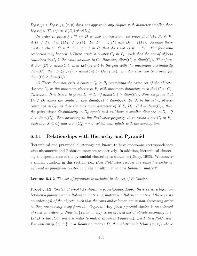
D2(x, y) > D1(x, y), (x, y) does not appear in any cliques with diameter smaller than

D2(x, y). Therefore, ψ(D1) 6= ψ(D2).

In order to prove ξ : P 7→ D is also an injection, we prove that ∀P1, P2 ∈ P,

if P1 6= P2, then ξ(P1) 6= ξ(P2). Let D1 = ξ(P1) and D2 = ξ(P2). Assume there

exists a cluster C with diameter d in P1 that does not exist in P2. The following

scenarios may happen i)There exists a cluster C2 in P2, such that the set of objects

contained in C2 is the same as those in C. However, diam(C) 6= diam(C2). Therefore,

if diam(C) > diam(C2), then Let (x1, x2) be the pair with the maximum dissimilarity

diam(C), then D1(x1, x2) > diam(C2) > D2(x1, x2). Similar case can be proven for

diam(C) < diam(C2)

ii) There does not exist a cluster C2 in P2 containing the same set of the objects.

Assume C2 be the minimum cluster in P2 with minimum diameter, such that C1 ⊂ C2.

Therefore. It is trivial to prove D1 6= D2 if diam(C1) ≥ diam(C2). Now we prove that

D1 6= D2 under the condition that diam(C1) < diam(C2). Let X be the set of objects

contained in C1, let d be the maximum diameter of X by D2. If d = diam(C2), then

the pairs whose dissimilarity in D2 equals to d will have a smaller distance in D1. If

d < diam(C2), then according to the PoCluster property, there exists a set C ′2 in P2,

such that X ⊆ C ′2 and diam(C ′

2) == d, which contradicts with the assumption.

6.4.1 Relationships with Hierarchy and Pyramid

Hierarchical and pyramidal clusterings are known to have one-to-one correspondences

with ultrametric and Robinson matrices respectively. In addition, hierarchical cluster-

ing is a special case of the pyramidal clustering as shown in (Diday, 1986). We answer

a similar question in this section, i.e., Does PoCluster recover the same hierarchy or

pyramid as pyramidal clustering given an ultrametric or a Robinson matrix?

Lemma 6.4.2 The set of pyramids is included in the set of PoCluster.

Proof 6.4.2 (Sketch of proof) As shown in paper(Diday, 1986), there exists a bijection

between a pyramid and a Robinson matrix. A matrix is a Robinson matrix if there exists

an ordering θ of the objects, such that the rows and columns are in non-decreasing order

as they are moving away from the diagonal. Any given pyramid cluster is an interval

of such an ordering. Now let {x1, x2, ..., xn} be an ordered list of objects according to θ.

Let D be the Robinson dissimilarity matrix shown in Figure 6.4. Let P be a PoCluster.

For any entry {xi, xj} in a Robinson matrix D, the sub-triangle below {xi, xj} above

105

the main diagonal corresponding to the rows 〈xi, ..., xj〉 and the columns 〈xi, ..., xj〉 will

contain lesser dissimilarity values than D(xi, xj), therefore, {xi, ..., xj} will be a cluster

in P , which is an interval of θ. Therefore, starting from the entries from the upper

right corner, then recursively traversing the two lower sub-triangles 〈xi, ..., xj−1〉 and

〈xi+1, ..., xj〉 returns the whole pyramid, which is also a PoCluster.

6.5 PoCluster Derivable Ontology

In practice, a classification taxonomy can be an arbitrary collection of sets, referred to

as poset, where neither the diameters of the clusters nor the pair-wise dissimilarities be-

tween objects are available. In this section, we address a particular subset of posets. A

poset is PoCluster derivable if applying PoClustering to a dissimilarity matrix generates

the same set of clusters. A PoCluster derivable poset can be considered as a PoClus-

ter of which the diameter information is unknown. Therefore, each PoCluster derivable

poset corresponds to a infinite collection of PoClustersthat contain the same clusters

but with different diameters.

However, not every poset is PoClusterderivable. For example, let Q represent a set

of object sets, Q ∈ 22N . A poset Q containing 4 clusters, i.e. {AB,AC,BC,ABC}, is

not PoCluster derivable. Set {ABC} must have the same diameter of at least one of

two element subsets, {AB}, {AC}, or {BC}. Therefore, the two elements subset with

the same diameter as ABC cannot be a cluster in a PoCluster since it is not maximal.

Since each PoCluster corresponds to a unique dissimilarity matrix, it is possible to

derive dissimilarities or relative dissimilarities between objects in the PoCluster deriv-

able set.

In this section, we are particularly interested in how to determine whether an ar-

bitrary poset is PoCluster derivable and if it is, how the elements in the poset can be

used to derive the ranking of dissimilarity entries.

Definition 6.5.1 Let Q be a set over the sets of objects in N , i.e. , Q ∈ 22N . We say

Q is PoCluster derivable if there exists a PoCluster P of some dissimilarity matrix

D, such that Q is the set of clusters in P obtained by ignoring the cluster diameters.

In the following, we examine both necessary and sufficient conditions to identify Q

as a PoCluster derivable set.

We define 〈q1, q2, ..., qm〉 as a partition of the elements(clusters) in Q as follows. Each

element of Q (i.e. a subset of objects) appears in exactly one group qi of the partition.

106

We denote edges(qi) as all pairs of objects drawn from group qi. The partition has

the properties that each group qi is a subset of the elements in Q, the union of all the

groups is the universal set in Q, ∪mi>0qi = Q, and for any pair of groups (i, j), i 6= j,

qi ∩ qj = ∅.

Theorem 6.5.1 Q is PoCluster derivable, if and only if there exists an ordered parti-

tion of sets in Q, 〈q1, q2, ..., qm〉, such that ∀t, 1 < t ≤ m

qt = cliquesete(⋃

0<i≤t

edges(qi)) \ cliquesete(⋃

0<j<t

edges(qj)). (6.2)

Proof 6.5.1 First, we prove its sufficiency: Assume there exists an ordered partition

of the poset 〈q1, q2, ..., qm〉. We assign dissimilarity d(x,y) between two objects as the

following: {d(x, y) = 1, if e(x, y) ∈ edges(q1);

d(x, y) = t, if e(x, y) ∈ edges(qt) \ ∪0<i<t edges(qi).(6.3)

To prove Q is a PoCluster derivable, we prove that the sets in Q is equivalent to the

sets generated by ψ(D).

P = ∪0<t≤mcliquesetδ(d ≤ t) (6.4)

= ∪0<t≤mcliquesete(∪0<j≤tedges(qj)) (6.5)

= cliquesete(edges(q1)) ∪

∪1<t≤m(cliquesete(∪1<i≤tedges(qi)) \

cliquesete(∪1<j≤(t−1)edges(qj))) (6.6)

⇒ S(P ) = ∪0<i≤tqi

We next prove it is a necessary condition. If Q is PoCluster derivable, we want to

prove that the condition is true. Let D be the dissimilarity, which has the bijection with

Q, such that Q = S(p(D)). Assume that 〈d1, d2, ..., dm〉 is the dissimilarity coefficient in

D with increasing order. We can group the clusters according to the rank of the dissimi-

larities. Let q1 = cliquesetδ(d1). ∀1 < t ≤ m, let qt be the maximal clique with diameter

dt, which does not occur in qt−1, such that qt = cliquesetδ(dt) − cliquesetδ(dt−1) =

cliquesete(∪0<i≤tedges(qi)) \ cliquesete(∪0<j<tedges(qt)).

107

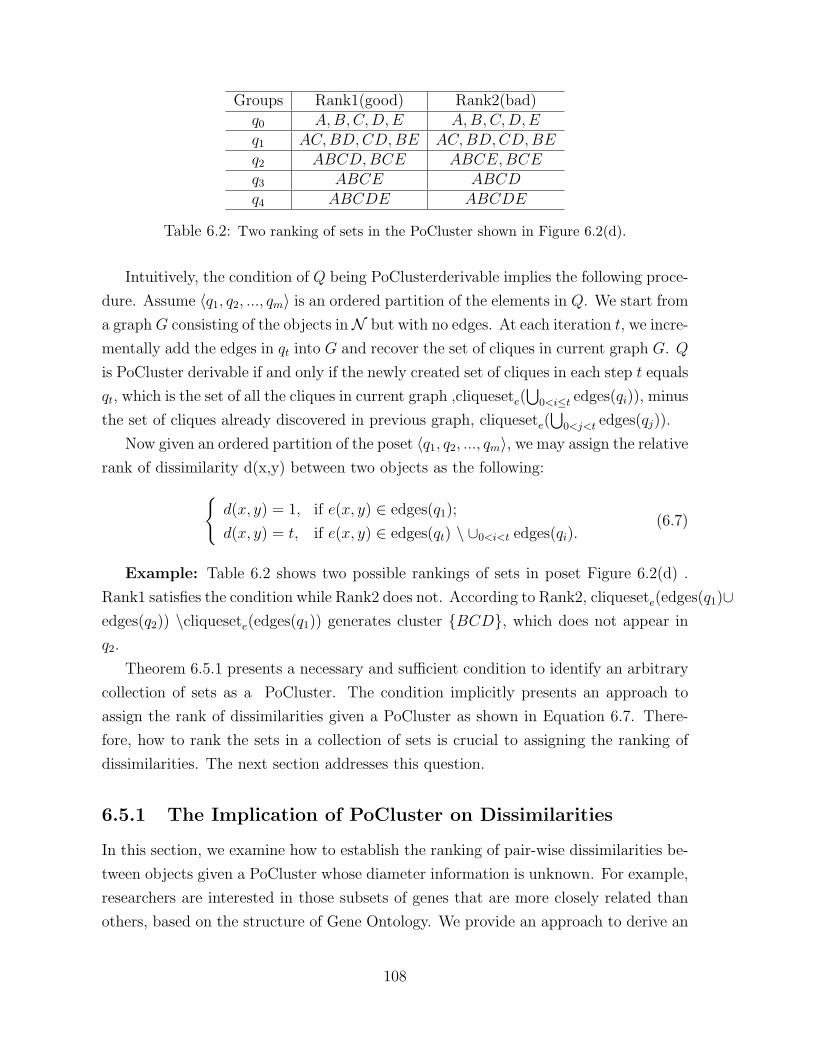
Groups Rank1(good) Rank2(bad)q0 A,B,C,D,E A,B,C,D,Eq1 AC,BD,CD,BE AC,BD,CD,BEq2 ABCD,BCE ABCE,BCEq3 ABCE ABCDq4 ABCDE ABCDE

Table 6.2: Two ranking of sets in the PoCluster shown in Figure 6.2(d).

Intuitively, the condition of Q being PoClusterderivable implies the following proce-

dure. Assume 〈q1, q2, ..., qm〉 is an ordered partition of the elements in Q. We start from

a graphG consisting of the objects inN but with no edges. At each iteration t, we incre-

mentally add the edges in qt into G and recover the set of cliques in current graph G. Q

is PoCluster derivable if and only if the newly created set of cliques in each step t equals

qt, which is the set of all the cliques in current graph ,cliquesete(⋃

0<i≤t edges(qi)), minus

the set of cliques already discovered in previous graph, cliquesete(⋃

0<j<t edges(qj)).

Now given an ordered partition of the poset 〈q1, q2, ..., qm〉, we may assign the relative

rank of dissimilarity d(x,y) between two objects as the following:{d(x, y) = 1, if e(x, y) ∈ edges(q1);

d(x, y) = t, if e(x, y) ∈ edges(qt) \ ∪0<i<t edges(qi).(6.7)

Example: Table 6.2 shows two possible rankings of sets in poset Figure 6.2(d) .

Rank1 satisfies the condition while Rank2 does not. According to Rank2, cliquesete(edges(q1)∪edges(q2)) \cliquesete(edges(q1)) generates cluster {BCD}, which does not appear in

q2.

Theorem 6.5.1 presents a necessary and sufficient condition to identify an arbitrary

collection of sets as a PoCluster. The condition implicitly presents an approach to

assign the rank of dissimilarities given a PoCluster as shown in Equation 6.7. There-

fore, how to rank the sets in a collection of sets is crucial to assigning the ranking of

dissimilarities. The next section addresses this question.

6.5.1 The Implication of PoCluster on Dissimilarities

In this section, we examine how to establish the ranking of pair-wise dissimilarities be-

tween objects given a PoCluster whose diameter information is unknown. For example,

researchers are interested in those subsets of genes that are more closely related than

others, based on the structure of Gene Ontology. We provide an approach to derive an

108

appropriate dissimilarity assignment between pairs in a PoCluster derivable clusters.

According to Theorem 6.5.1, in order to derive a dissimilarity rank of pairs as in

Equation 6.7, it is necessary to partition the set of clusters into ordered subgroups.

One of the basic principles for ranking sets is based on their subset relationships. In

this section, we further study the PoCluster properties to infer the set ranking.

Let S be a cluster in PoCluster P , and e be a pair in S × S. We say S is the

minimum cluster containing e if e is not contained in any subset of S. We denote S

as the sets of pairs for which S is a minimum cluster. The remaining pairs, which are

contained in at least one of S’s subsets, are denoted as S. The minimum cluster for

a pair is important since its diameter determines the pair’s dissimilarity. In addition,

a pair might exist in multiple sets, therefore, it is possible that there exists multiple

minimum clusters containing this pair. Given e as a pair, we denote the set of minimum

clusters containing e as e∗.

Example: According to the PoCluster from Figure 6.2 (d), set ABCE is the

minimum cluster containing the pair (A,E). Therefore, (A,E)∗ = {ABCE}, and

(A,B)∗ = {ABCE,ABCD}. In addition, ABCE = {(A,E), (A,B)}, and ABCE =

{(A,C), (B,C), (B,E), (C,E)}.

Corollary 6.5.1 Let P be a PoCluster and D be its corresponding, yet unknown, dis-

similarity matrix. For any set S in P ,

1. |S| 6= ∅;

2. Let e ∈ S, diam(S) > D(e).

3. Let e ∈ S, diam(S) ≥ D(e).

4. Let e ∈ S, diam(S) = D(e), if there only exists one minimal cluster containing

e(|e∗| = 1) or e is the only edge that S is a minimum cluster (|S| = 1).

Corollary 6.5.1 presents three relationships between the distance of pairs in a set S

and the set’s diameter. First, a set has to be a minimum cluster of a pair, i.e.,|S| 6= ∅,or it conflicts with property 2. Properties 2 and 3 provide order constraints between

any element within a set and the diameter of the set; property 4 identifies a way to

assign a pair-wise dissimilarity as the diameter of the set. We denote these pairs in a

set as diameter determinant pairs.

109

The following two corollaries determine the relative order between the diameters of

two clusters based on a shared edge following corollary 6.5.1. These two corollaries are

used in Algorithm 7 that follows.

Corollary 6.5.2 Let P be a PoCluster and D be its corresponding dissimilarity matrix,

then for any two clusters S1 and S2 in P , if one of S1’s diameter determinant pair e

also belongs to S2, then diam(S1) < diam(S2);

Corollary 6.5.3 Let P be a PoCluster and D be its corresponding dissimilarity matrix.

Let S be a cluster in P . If any pair e, e ∈ S, belongs to a cluster with diameter less

than δ, then diam(S) < δ.

6.5.2 Algorithm of Deriving Dissimilarities

In this section, we present an algorithm to identify whether an input poset is a PoClus-

ter derivable set. It also derives a relative ranking of pair-wise dissimilarities simulta-

neously.

The algorithm proceeds in a top-down fashion and the diameter is reduced in each

step. In each step, the algorithm first identifies the maximum set of independent object

sets. By independent, we mean that the sets are not subsets of another. It then removes

those clusters from current maximum independent sets that have lower diameters. The

remaining sets are then assigned the current diameter and are removed from the current

pool of sets. The process repeats until all sets are assigned diameters, or the collection

of sets is invalidated as PoCluster.

Function getMaxTopSets first extracts the maximum independent sets within the

current poset P t, denoted by >. This step follows the basic property of PoCluster,

which states that a superset of a set has a larger diameter.

Next, function removeLowerRankSet removes any sets that have lesser diameter

than one of the sets in current >. One criterion is based on Corollary 6.5.2. If one

determinant pair of a set S1 appears as lower ranked pair in another set S2 of current

>, then S1 is removed. The second criterion is based on Corollary 6.5.3. If for any top

ranked pair e in a set S1, e ∈ S1, there exists a set S2 in >, such that e is lower ranked

e ∈ S2, then set S1 from the top will be moved to the lower ranked sets.

Finally, we check whether the rank of the set violates Theorem 6.5.1, in the function

checkCliques. If this is violated, the solution is to find a superset containing these

additional sets and put it into the bottom. If no such superset exists, then the poset is

110

not a PoCluster. However, this step requires the process to find all clique sets, which

has NP-complete complexity. Therefore, in practice, this step is usually approximated.

Of course, degenerate cases might arise due to the approximation and the recovered

dissimilarity might not be exactly faithful to the poset.

If all checks are passed, then we assign those pairs contained solely in the top

part > dissimilarities equal to the current diameter δ. Failure of any of the above

steps invalidates the poset as a PoCluster. The procedure continues by reducing the

diameter and removing the top from the remaining poset. It stops when the current

pool is either empty or unchanged between successive iterations. If the pool remains

unchanged, the poset is not PoCluster derivable set.

Algorithm 7 RankPoset: Deriving dissimilarity from posetInput: P : A posetOutput: D: Dissimilarity matrix derived from P

1: t← 1; P t ← P ; P0 ← ∅2: diamt ← 1

2|N | ∗ (|N | − 1);

3: while (P t 6= P t−1)&(P t 6= ∅) do4: > = getMaxTopSet(P t);5: > = removeLowerRankSet(P t,>);6: > = cliqueCheck(P t,>);7: D(e)← diam, ∀e, where e ∈ P t \ >8: t← t+ 1;P t ← P t−1 −>; diamt ← diamt−1;9: end while

10: return D.

Example 6.5.1 The following steps can be taken in order to derive the dissimilarity

matrix of PoCluster in Figure 6.2 (d).

1. Starting from the maximal set ABCDE when t = 1, the diameter can be set to

10, since all the sets are its children. g′1 = ABCDE will be removed from the

poset, and the program will continue to the next iteration t = 2.

2. Next, the maximal independent sets include ABCD and ABCE. And Elow =

{BC,BD,BE,AC,CD,CE}. Since no maximal pairs appear in Elow, therefore,

no set is removed. So both ABCD and ABCE are inserted in >1. Then, we com-

pute the cliquesete(Elow) and check whether it results in any additional sets. The

completeness check finds the additional set BCD in the cliqueseteElow, therefore,

a superset of BCD will have to be removed from >2, which would be ABCD,

(i.e., g′2 = ABCE).

111

3. Among the rest of poset, the maximal independent sets includes ABCD and

BCE. None of them has determinant pairs. The current Elow = {BC,CD,AC,BE}.And cliquesete(Elow) contains all the sets in the ABCD and BCE’s children, so

completeness check is passed. Therefore, ABCD and BCE both can be placed

in g′3.

4. The rest of sets are maximal and serve as determinant pairs for themselves. There-

fore, they are assigned to g′4.

5. The order of groups are reversed and rearranged in the increasing order of the

diameter. The final result appears in Table 6.2.

6.6 PoClustering Algorithm

Given a dissimilarity matrixD, the corresponding PoCluster P (i.e., P = {cliquesetδ(d)|∀d ∈W (D)}) can be found by repeating a simple procedure. In the naive algorithm, one

needs only to find all cliques in a subgraph of G(D) that includes only those edges

corresponding to the pair-wise dissimilarities less than or equal to a threshold d as the

threshold varies from the smallest to the largest dissimilarity in D.

An incremental and exact PoClustering algorithm was proposed by (J. Liu and

Prins, 2006). The algorithm only computes clique clusters that are affected by the

introduction of new edges. The algorithm maintains a pool of all clusters in the previous

graph. Given the next graph with more edges, the pool of cliques can be updated as

follows: First, all the cliques in the pool that share a vertex with the new edges are

found. Second, if a clique in the pool can be extended by adding one or more of the new

edges, the extended clique is added to the pool, and the cliques that are subgraphs of

the new clique are removed. The parent-child relationships can be established between

new cliques and removed cliques.

Though more efficient, the exact algorithm still bears the NP-Complete complexity

of the PoClustering problem because of the search of clique clusters. In addition,

the number of clique clusters in a undirected graph with n nodes is o(31/3∗n). Most

real classifications are polynomial posets, which means the number of clusters in the

poset is polynomial with respect to the number of objects. In this section, we present

a heuristic algorithm for the construction of approximate PoClusters. This approach

addresses both the NP-completeness of finding all cliques and the huge number of clique

clusters generated.

112

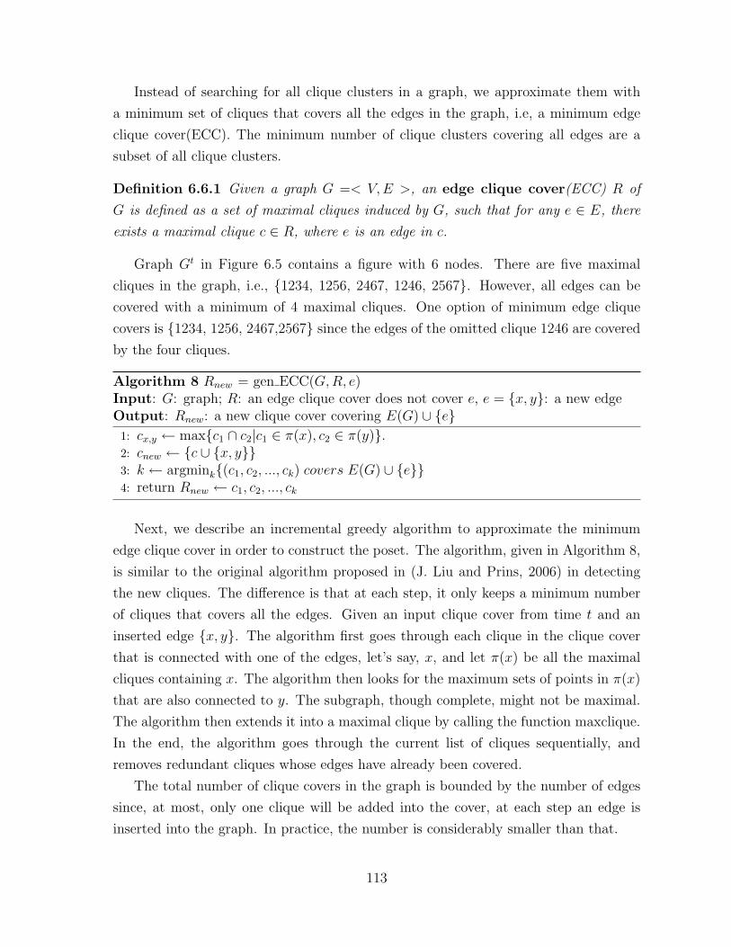
Instead of searching for all clique clusters in a graph, we approximate them with

a minimum set of cliques that covers all the edges in the graph, i.e, a minimum edge

clique cover(ECC). The minimum number of clique clusters covering all edges are a

subset of all clique clusters.

Definition 6.6.1 Given a graph G =< V,E >, an edge clique cover(ECC) R of

G is defined as a set of maximal cliques induced by G, such that for any e ∈ E, there

exists a maximal clique c ∈ R, where e is an edge in c.

Graph Gt in Figure 6.5 contains a figure with 6 nodes. There are five maximal

cliques in the graph, i.e., {1234, 1256, 2467, 1246, 2567}. However, all edges can be

covered with a minimum of 4 maximal cliques. One option of minimum edge clique

covers is {1234, 1256, 2467,2567} since the edges of the omitted clique 1246 are covered

by the four cliques.

Algorithm 8 Rnew = gen ECC(G,R, e)Input: G: graph; R: an edge clique cover does not cover e, e = {x, y}: a new edgeOutput: Rnew: a new clique cover covering E(G) ∪ {e}1: cx,y ← max{c1 ∩ c2|c1 ∈ π(x), c2 ∈ π(y)}.2: cnew ← {c ∪ {x, y}}3: k ← argmink{(c1, c2, ..., ck) covers E(G) ∪ {e}}4: return Rnew ← c1, c2, ..., ck

Next, we describe an incremental greedy algorithm to approximate the minimum

edge clique cover in order to construct the poset. The algorithm, given in Algorithm 8,

is similar to the original algorithm proposed in (J. Liu and Prins, 2006) in detecting

the new cliques. The difference is that at each step, it only keeps a minimum number

of cliques that covers all the edges. Given an input clique cover from time t and an

inserted edge {x, y}. The algorithm first goes through each clique in the clique cover

that is connected with one of the edges, let’s say, x, and let π(x) be all the maximal

cliques containing x. The algorithm then looks for the maximum sets of points in π(x)

that are also connected to y. The subgraph, though complete, might not be maximal.

The algorithm then extends it into a maximal clique by calling the function maxclique.

In the end, the algorithm goes through the current list of cliques sequentially, and

removes redundant cliques whose edges have already been covered.

The total number of clique covers in the graph is bounded by the number of edges

since, at most, only one clique will be added into the cover, at each step an edge is

inserted into the graph. In practice, the number is considerably smaller than that.

113

The number of outer loop iterations of the algorithm are determined by the number

of edges, which is O(n2). For a new clique, the greedy algorithm goes through the

cliques in the existing clique cover, and find the maximal clique cover. Assume the

number of cliques in the cover is k, creating a maximal clique takes O(kn). Checking

the coverage of edges by the cliques also takes o(kn2) time.

6.7 Experiments

We have experimented with both synthetic and real datasets comparing hierarchical

clustering(Hierarchy), pyramidal clustering(Pyramid), and edge clique cover(ECC). We

do not present the results of the exact algorithm because of its prohibitively long

running time.

6.7.1 Evaluation Criteria

The match score is used to measure the approximation of the recovered poset to the

original poset. We take each poset as a set of sets. Given two PoClusters P1 and P2,

the match score of P2 to P1 is computed as:

match(P1, P2) = means1∈P1(maxs2∈P2(|s1 ∩ s2||s1 ∪ s2|

)) (6.8)

For each set in P1, only the best match in P2 is taken account of by Jaccard coef-

ficient. The overall match score is determined by the mean match score of the whole

sets.

6.7.2 Synthetic Data

We created a synthetic poset generator that is controlled by three parameters. They

are the number of objects of the universal set N , the total number of clusters (sets), and

the overlap probability between clusters. The overlap probability follows a normal dis-

tribution with a user-specified mean value and a default standard deviation of√

(0.2).

It defines the likelihood that an element in a parent cluster appears in more than one

child cluster. The synthetic generator of the poset then works as follows: starting from

the root node of the poset with n objects, the program recursively generates the child

sets that respect the overlap probability distribution. For each parent set, whether an

object should appear in multiple child sets is determined by coin-flipping with overlap

114

probability poverlap. After the poset is generated, we computed the rank and assigned

the pair-wise distances based on the algorithm presented in Section 6.5.2. We then take

the distance matrix as the input to the three clustering algorithms.

We first examined how the overlap probability affects the performance. In this

setting, the total number of objects in N is set to 500, and the maximum number of

clusters in P is 200. Figure 6.6(A) shows that overlap probability affects match score

of all three algorithms. Starting from 0 overlap, all of the three algorithms have almost

100% match score. However, ECC does a much better job than the other two. The

reason is that the number of overlapping clusters increases as the overlap probability

increases. The match score drops significantly for hierarchical and pyramidal clustering

because of their inability to allow arbitrary overlaps between clusters. Figure 6.6(B) and

(C) show the total number of clusters generated and the running time comparison. Both

hierarchical clustering and pyramidal clustering have shorter running time than ECC.

It is due to the fact that both algorithms fail to recover most clusters in the original

poset. This can be observed from Figure 6.6(B) where, among the three algorithms,

ECC is the only one that is able to recover most clusters in the original poset (its

number of clusters is shown as the top curve in Figure 6.6(B)) .

Our second experiment demonstrated how the number of objects affects the perfor-

mance. The overlap probability is set to 0.2 and maximum number of clusters is 120.

The results are shown in Figure 6.6 (D), (E), and (F). The match score is close to 1

for ECC but drops below 0.5 for the other two algorithms. Again, the difference in the

running time (Figure 6.6 (F)) between ECC and others is because both hierarchical

clustering and pyramidal clustering recover only a small fraction of the sets(clusters)

in the original poset (the top curve shown in Figure 6.6 (E)).

In the last experiment, we fixed the number of objects to 500 and the overlap

probability to 0.2, and varied the number of clusters in the poset. The result are shown

in Figure 6.6 (G) and (H). A side effect of increasing the number of clusters defined

on a fixed set of objects is an increase in the degree of overlap. Therefore, the match

scores of hierarchical clustering and pyramidal clustering fall as the number of clusters

increases, whereas ECC maintains a high match score. As shown in Figure 6.6 (H),

ECC is able to recover almost all clusters in the original poset. However, pyramidal

clustering and hierarchical clustering generate considerably fewer clusters.

115

6.7.3 Gene Ontology

Our next experiment compares the quality of the three clustering algorithms given a

real ontology categorization. We also compare our method for deriving dissimilarities

with the previous approaches reviewed in Section 6.2.

We used 2884 genes, which are the most active and co-regulated in the yeast cell

cycle data selected by Tavazoie et al. (1999)(Tavazoie et al., 1999). This set of genes

has been frequently studied. Therefore, we expect most of them to have comprehen-

sive annotations and classifications. We consider three GO files: biological process

(BP), cellular component (CC), and molecular function (MF), from the Gene Ontology

databases. We extracted all GO categories that contain at least two genes from the

identified set and removed duplicate categories. The remaining GO categories are used

to generate dissimilarity matrices as the input to the clustering algorithms. Table 6.3

presents size and overlap statistics of our data. The statistics of the three GO files are

shown in Table 6.3.

GOfiles

#Knowngenes

#Terms

Maxlevel

MeanOver-lap

BP 1313 2631 18 37%CC 1316 1142 14 22%MF 1309 624 17 31%

Table 6.3: Statistics for the three GO files. MF: Molecular Function, CC: Cellular Compo-nent; BP: Biological Process

The result of applying the three algorithms is consistent with that of the synthetic

data. ECC performs the best in recovering Gene Ontologies. In this case, two ad-

ditional measurements are used to evaluate the relationships between a reconstructed

poset(P ) and GO files(go). Besides the match score, we also look at recovery rate and

accuracy. The recovery rate is the percentage of GO categories recovered; the accu-

racy is the percentage of the discovered clusters that actually appear in GO categories.

The two measurements provide more information about those clusters. As shown in

Table 6.5, more than 50% and even closer to 79%(MF) of the categories cannot be

properly discovered by hierarchical and pyramidal clustering. Meanwhile, according

to the third column in the same table, over 96% of the discovered clusters by ECC

are actual matches to the GO categories. In comparison, the spuriousness clusters in

116

pyramidal clustering and hierarchical clustering exceeds 50%, which is unacceptable for

real applications.

Similarity BP CC MFRankPoset 0.8473 0.8976 0.8031Resnik 0.7917 0.8601 0.7761LC 0.5466 0.7268 0.6724

Table 6.4: Reconstructed poset match score to original GO based on various similaritymeasures

match score recovery rate accuracyAlgoECCPyra.Hier.

BP CC MF0.8299 0.8976 0.88310.5367 0.4923 0.67350.4577 0.4260 0.5262

BP CC MF0.7813 0.8953 0.82730.3931 0.4704 0.46510.2779 0.4392 0.4175

BP CC MF0.9352 0.9534 0.99320.4504 0.6345 0.60230.3733 0.5702 0.4645

Table 6.5: Reconstructed poset match score to original GO by the three algorithms. go

represents the GO file and P is the reconstructed poset

We also compared the three different (dis)similarity measures including the RankPoset,

which we developed in Section 6.5.2, Resnik, and Leacock and Chodorow (LC) (Budanitsky,

2001). We computed three dissimilarity matrices, one by each method. We then applied

ECC algorithm to each of them. The matching score is shown in Table 6.4. Our RankPoset

generates a slightly better result than Resnik, while both are substantially better than LC.

6.8 Conclusions

PoClustering can be used for automatic construction ontologies based on the pairwise rela-

tionships between objects. PoClustering represents a one-to-one correspondence between all

possible dissimilarity matrices and a subset of posets, which we call the PoClusters. The

clustering approach preserves all of the information in a dissimilarity matrix, and we have

shown algorithms in both directions — constructing a PoCluster from dissimilarities, and

assigning meaningful dissimilarity values to any given PoCluster .

PoClusters are a generalization of both hierarchical clustering and pyramid clustering.

PoClusters provide both homogeneity within a cluster, as measured by the cluster’s diameter

as well as separation between clusters. They are also able to handle overlaps in a meaningful

way.

117

The formal definition of PoClusters is primarily of theoretical interest, since the problem

of computing them exactly is likely to be intractable for large problems. To address this short-

coming we have introduced a polynomially bounded approximation algorithm to automati-

cally generate classification hierarchies. Classification hierarchies are useful for automatically

generating categorizations, taxonomies, and ontologies in a wide range of applications.

Alternatively, our mapping from PoCluster to dissimilarity provides a meaningful pair-

wise dissimilarity measure between objects in taxonomies. At the very least, the resulting

dissimilarity matrix, when coupled with our new clustering algorithm, is capable of exactly

reconstructing a hierarchical set of clusters identical to the original categories, both in terms

of the subsets generated and their parentage.

118

(a) Dissimilarity

(b) Weighted graph

(c) Clique Clusters

(d) PoCluster.

Figure 6.2: A running example. (a) shows a dissimilarity matrix of 5 objects {A, B, C, D, E};(b) shows an undirected weighted graph implied by (c); Table (c) contains the list of cliqueclusters with all diameters; (d) shows a PoCluster which contains 13 clusters and their subsetrelationships (Each cluster in the PoCluster represents a clique cluster with its diameter in(c). The PoCluster is organized in DAG with subset relationship between the nodes. Thereis a directed path from node S1 to S2 if S1 ⊂ S2). Note: Applying PoClustering algorithmcan construct PoCluster shown in (d) given dissimilarity matrix (a). Applying Algorithm inSection 6.5.2 can derive the dissimilarities in (a) from PoCluster in (d).

119

A

C

B

D

E2

11

1

3

21

4

2

A

C

B

D

E11

1

1

A

C

B

D

E

2

11

1

21

2

A

C

B

D

E

2

11

1

3

21

2

d = 1 d = 2 d = 3 d = 4

22 2

Figure 6.3: Four directed weighted graphs corresponding to the dissimilarity matrix in Fig-ure 6.2 (B) with maximum edge weight {d = 1, 2, 3, 4}.

X iXj

Dij

X 1

X1Xn

Xn

X iXj

X i Xj

0 0 0 0 0 0 0 0 0 01 1 2 1 2 1 2 3

2 2 3 3 3 4 3 43 4 4 5 6 5 7

5 6 6 7 7 97 7 8 8 11

8 9 10 13

10 12 1514 18

20

1

Figure 6.4: A structure of Robinson matrix. There exists a linear ordering of the objects,such that the dissimilarity never decreases as they move away from diagonal along both rowand column.

1

2

3

4

5

6

7

Figure 6.5: An example graph with nodes {1,2,3,4,5,6,7}. All the cliques in the graph are{1234, 1256, 2467, 1246, 2567}; The Minimum ECC is {1234, 1256, 2467, 2567}.

120

A D

B E

C F

G H

Figure 6.6: Experimentation on synthetic data

121

Chapter 7

Visualization Framework to Summarize and

Explore Clusters

Subspace clustering has proven itself as a useful data-mining tool for finding significant re-

lationships within high-dimensional data. However, exploring the potentially exponential

number of identified subspace clusters is unwieldy and presents it own data mining chal-

lenges. Inspecting subspace clusters for meaningful relationships is like searching for a needle

in a haystack.

In this chapter, we build a visualization framework to aid the analysis of the entire set

of subspace clusters mined from a given dataset. We develop measures to establish pairwise

dissimilarities between subspace clusters. These measures incorporate notions of coverage

between the subspace clusters, as well as how similar the exhibited patterns of the pair are.

Dissimilarity measures are requisite for our visualization and clustering analysis (i.e. clusters

of subspace clusters). We present our experience with the visualization framework on two

real datasets.

7.1 Introduction

Subspace clustering (Agrawal et al., 1998; Yang et al., 2002; Ben-Dor et al., 2002) is an effec-

tive method for finding meaningful homogeneous groups within lower-dimensional subspaces

of high-dimensional data. It has been widely used in bioinformatics applications, such as gene

expression analysis (Ben-Dor et al., 2002; Cheng and Church, 2000). However, the usefulness

of subspace clustering algorithms are often overshadowed by the multitudes of results they

generate. The lack of efficient interpretation tools often keeps domain experts from making

sense of the results. The motivation for our work is to organize and summarize the results

of subspace clustering. We achieve this by constructing an analogy of a subspace cluster

as a point in an abstract data space, where various relationships between points (subspace

clusters) are analogous to proximity. We then employ a visualization interface to explore

relationships between and filter subspace clusters.

Figure 7.1: Left: A visualization of the overlap between the yellow and blue sets ofsubspace clusters as shown in the image on the right. The intersection of the two setsof subspace clusters is shown in green. There are over 10 subspace clusters in each set.Right: The 3D point-cloud view of subspace clusters.

A subspace cluster can be thought as a combination of a binary selection pattern with an

analog pattern imposed on it. In the binary matrix, a submatrix of 1s indicates the presence

of the item-feature pair within the submatrix. Correlations between the signals superimposed

on this submatrix validate it as a subspace cluster. Random noise can exclude an item or

feature out of the subspace cluster, which is equivalent of turning the corresponding entry

into 0.

Subspace clustering algorithms often generate thousands, or even tens of thousands of

clusters. However, many of the discovered relationships within a subspace cluster are either

trivial or highly redundant relative to others. Researchers tend to address the problems of

excessive and mundane subspace clusters by varying thresholds, which indeed reduce the

number of outputs and increase pattern variations, but at a cost of masking potentially

significant results.

Subspace clusters are frequently highly overlapped, due to the overlapping nature of sub-

spaces and the well known A-priori property. We show an example of this in Figure 7.1.

Figure 7.1 shows 2 sets of clusters, colored blue and yellow, which are highly overlapped. The

colorbars to the left and top of the left panel indicate which rows and columns, respectively,

belong to which subspace cluster. Their intersection is shown in green (mixing blue and yellow

makes green). The dominance of the green in the colorbar indicates a high level of overlap,

and is one aspect of our visualization tool. If a set of items does not form a subspace cluster

in subspace S, then this set of items, and any subset of them, won’t form a cluster in any

superspace of S.

Moreover, the generated subspace clusters are often fragments of logarithmic size with

respect to original subspace clusters according to our previous study in (Jinze Liu and Prins,

123

2006).

These characteristics present tremendous challenges for applying subspace clustering meth-

ods and understanding their results. We propose an abstract mapping of subspace clustering

results to a geometric analogy, and employ visualization methods to address these challenges.

Our approach requires meaningful pairwise metrics to compare relationships between sub-

space clusters, scalable visualization techniques, and tools for exploring the results. We make

the following contributions:

• We define and justify a set of useful pair-wise relationships between subspace clusters.

These relationships include notions of coverage similarity and pattern similarity.

• We develop a geometric analogy where the subspace clusters generated from any given

algorithm are treated as point and the relationships between them are treated as dis-

tances. This allows us to find patterns, and in fact, cluster subspace clusters into similar

groups.

• We build a visualization framework to support our geometric analogy. This allows us to

visualize and interact with the points, and their clusters. Our visualization tool makes

the abstract notations of our model concrete. Our visualization is further enabled by

a scalable algorithm that we have developed, fastMDS, for supporting the interactive

display of large subspace-cluster datasets.

7.2 Related Work

Visualizing the results of clustering algorithms can provide many insights about the data, as

well as the clustering algorithm itself. For instance, a visualization may help in verifying the

accuracy of a clustering algorithm, as well as give a user some intuition for what parameters

to use and further experiments to try. Thus, there are many different ways to visualize a

clustering solution.

7.2.1 Cluster and Subspace Cluster Visualization

Cluster visualization methods have been studied for years to assist the interpretation of clus-

tering results. However, previous cluster visualizations have often been limited to full dimen-

sional clustering, such as hierarchical clustering(Seo and Shneiderman, 2002) and K-means

clustering(Spence, 2001). In full dimension clustering, the difference among the clusters are

only in the object sets. To visualize them, people often project them onto a low dimen-

sional space and color them according to class labels. As for hierarchical clustering, the tree

structured dendrogram is often used as the visualization tool.

124

While there has been much work on visualizing traditional full space clusters, there has

been relatively little work done on visualizing subspace clusters. The visualization of subspace

clusters has been complicated by their overlapping nature. As a result it is difficult to visualize

the objects using just cluster labels in low dimensional space without ambiguity. Therefore, in

current literature on subspace clustering, people often plot the pattern or the sets of objects

in each subspace cluster separately. For example, each gene expression cluster generated by

Cheng et.al.(Cheng and Church, 2000) is shown as a line graph, where the line plots a gene’s

expression value under the set of conditions in the subspace cluster. In addition, a cluster

of data objects can also be projected onto pairs of features and plotted as points in 2D. If

points are separated by certain features, peaks are exhibited in density plots of the data in

those dimensions(Parsons et al., 2004).

7.2.2 Postprocessing of Subspace Clusters

The postprocessing of large amounts of clusters has been used recently in identifying repre-

sentatives of frequent itemsets. The work by Afrati et.al.(Afra-ti et al., 2004) finds the top-k

itemset that can cover the whole border of the frequent itemset. Yan et.al.(Yan et al., 2005)

improves it by taking the statistical support of each itemset into account.

The compression of subspace clusters is a more general problem than that of frequent

itemset in the following aspects: first, subspace clusters have pattern associated with them.

Finding representative sets that are both faithful and noise tolerant with respect to the original

pattern is a challenging problem. While frequent itemsets only take into account the set of

items, a subspace cluster considers either sets of rows or columns, or both, depending on the

application.

7.3 Model

We consider the set of subspace clusters that is output from subspace clustering algorithms.

First, we give a general definition of subspace clusters. We then define two measures of dissim-

ilarities between a pair of subspace clusters based on their coverage and pattern consistency.

Neither of the dissimilarity measures alone can perfectly represent the relationships between

two subspace clusters. Therefore, we also propose a linear combination of two measures of

dissimilarity.

7.3.1 Subspace Cluster

A subspace cluster is a subset of objects, which exhibits consistent patterns along a subset

of conditions. Assume M is an n by m matrix which contains a set of objects(rows) I0 =

125

{i1, i2, ..., in} and a set of attributes(columns) J0 = {j1, j2, ..., jm}. Each entry value Mi,j

represent the value of the object i under attribute j.

A subspace cluster P in M is depicted by a tuple 〈I, J, P 〉. I is a subset of objects, I ∈ I0

and J is a subset of attributes J ∈ J0(so-called subspace). P is the consistency measure of

the set of objects in I in subspace J .

In this paper, we focus on maximal subspace clusters. By maximal, we mean that adding

any additional row or column from the rest of matrix will violate the consistency measure

of the cluster. Since non-maximal subspace clusters are easy to filter out, in the rest of

discussion, we only consider the maximal subspace clusters.

Figure 7.2: The relationships between two overlapping clusters. The green and bluerectangles represent two separate subspace clusters. The yellow region is the intersec-tion of two. The whole region including green, blue, yellow and white is the merged(or unioned) cluster of the two clusters.

7.3.2 Coverage Dissimilarity

One relevant way to measure dissimilarities between subspace clusters is to measure the

diversity of set of objects and the set of attributes they contain. One well known measure

that serves this purpose is the Jaccard distance.

Definition 7.3.1 Given two subspace clusters C1 = 〈I1, J1〉 and C2 = 〈I2, J2〉, the coverage

dissimilarity between C1 and C2 is defined as

cDis(C1, C2) = 1− |I1 ∩ I2| × |J1 ∩ J2||I1 ∪ I2| × |J1 ∪ J2|

(7.1)

Figure 7.2 shows how two clusters can overlap. The green area is the coverage of cluster

1 (I1× J1) and the blue area is the coverage of cluster 2 (I2× J2). The intersection of cluster

1 and cluster 2 is shown in the the yellow area (I1 ∩ I2)× (J1 ∩ J2). And (I1 ∪ I2)× (J1 ∪ J2)

is the merged area.The coverage dissimilarity is computed as the percentage of uncommon

area in the merged area versus the merged area.

126

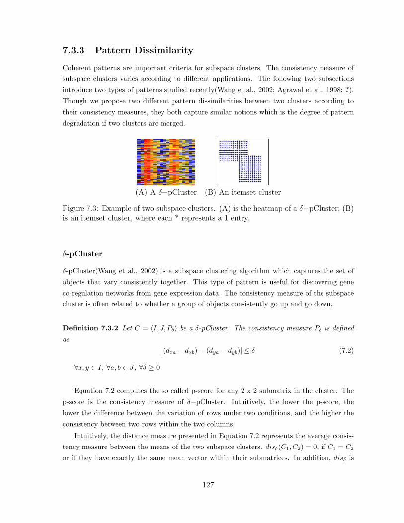
7.3.3 Pattern Dissimilarity

Coherent patterns are important criteria for subspace clusters. The consistency measure of

subspace clusters varies according to different applications. The following two subsections

introduce two types of patterns studied recently(Wang et al., 2002; Agrawal et al., 1998; ?).

Though we propose two different pattern dissimilarities between two clusters according to

their consistency measures, they both capture similar notions which is the degree of pattern

degradation if two clusters are merged.

(A) A δ−pCluster (B) An itemset cluster

Figure 7.3: Example of two subspace clusters. (A) is the heatmap of a δ−pCluster; (B)is an itemset cluster, where each * represents a 1 entry.

δ-pCluster

δ-pCluster(Wang et al., 2002) is a subspace clustering algorithm which captures the set of

objects that vary consistently together. This type of pattern is useful for discovering gene

co-regulation networks from gene expression data. The consistency measure of the subspace

cluster is often related to whether a group of objects consistently go up and go down.

Definition 7.3.2 Let C = 〈I, J, Pδ〉 be a δ-pCluster. The consistency measure Pδ is defined

as

|(dxa − dxb)− (dya − dyb)| ≤ δ (7.2)

∀x, y ∈ I, ∀a, b ∈ J , ∀δ ≥ 0

Equation 7.2 computes the so called p-score for any 2 x 2 submatrix in the cluster. The

p-score is the consistency measure of δ−pCluster. Intuitively, the lower the p-score, the

lower the difference between the variation of rows under two conditions, and the higher the

consistency between two rows within the two columns.

Intuitively, the distance measure presented in Equation 7.2 represents the average consis-

tency measure between the means of the two subspace clusters. disδ(C1, C2) = 0, if C1 = C2

or if they have exactly the same mean vector within their submatrices. In addition, disδ is

127

symmetric, since disδ(C1, C2)=disδ(C2, C1).

disδ(C1, C2) (7.3)

=1

12 |J ||J − 1|

j1<j2∑j1,j2∈J

|(dI1j1 − dI2j1)− (dI1j2 − dI2j2)|

where J is union of J1 and J2, and

dIj =1|I|∑i∈I

dij (7.4)

Itemset Cluster

Frequent itemset mining can be considered a special branch of subspace clustering meth-

ods. It looks for an itemset that is contained in a sufficient number of objects. In binary

representation, a ”1” entry corresponds to the presence of an item in the objects and a ”0”

corresponds to the absence. A frequent itemset corresponds to a submatrix of all 1s, as shown

in Figure 7.3(B).

Definition 7.3.3 (Itemset Cluster) The submatrix I × J is a itemset cluster if ∀ i ∈ I, ∀j ∈ J , Mi,j = 1 and |I|

|I0|≤δ , where δ is the minimum support threshold, 0 ≤ δ ≤ 1.

The pattern degradation due to merging two subspace clusters can be often measured by

the difference of the fraction of 1s in each of the union columns.

disitem(C1, C2) (7.5)

=1|J |

∑j∈J

|dIj1 − dIj2 |

where diJ is defined the same as Equation 7.4

It so happens that the mean of the itemset cluster is the same as the probability of seeing

a 1 entry in that column. The mean of the itemset clusters can be taken as a distribution

vector, and either the KL divergence or Jensen-Shannon divergence (Yan et al., 2005) can be

used to measure the pattern dissimilarity between the two clusters. This method is the same

as the approach taken by Yan et.al.(Yan et al., 2005).

7.3.4 Blending of Dissimilarities

Neither coverage dissimilarity nor pattern dissimilarity alone are perfect. They capture dif-

ferent aspects of dissimilarity between subspace clusters. Sometimes mixtures of the two may

128

reveal better separation of the clusters than either can alone. We allow different combinations

of dissimilarity measures to be used by assigning different weights to the coverage and pattern

dissimilarities.

7.3.5 View of A Set of Subspace Clusters

Given a set of closely related subspace clusters, we define two types of simplifications to de-

scribe them. One is a summary of the data, which contains the union of the rows and columns

of all subspace clusters in the set. In addition, we find a representative subspace cluster, de-

fined as the medioid of the set of clusters. The medioid has the property of minimizing the

sum of the dissimilarity from it to any of the subspace clusters in the set of subspace clusters.

Figure 7.4: The top row of matrices (a),(b),(c) represent pattern dissimilarity. Thebottom row (d),(e),(f) represents coverage dissimilarity. (a) The original pattern dis-similarity matrix; (b) Permuted pattern dissimilarity matrix, based on the clustering ofsubspace clusters by pattern dissimilarity alone; (c) Permuted pattern dissimilarity ma-trix based on the clustering by a 50/50 blend of both pattern and coverage dissimilarity;(d) The original coverage dissimilarity matrix; (e) Permuted coverage dissimilarity ma-trix, based on clustering subspace clusters on just coverage dissimilarity; (f) Permutedcoverage dissimilarity matrix based on a 50/50 blend of both pattern and coverage dis-similarity; (g) Blended Matrix of both pattern dissimilarity and coverage dissimilarity,permuted to show clustering

129

7.4 Methods

Although the visualization of dissimilarity matrices, provides useful insights, it is not natural

enough for human to identify possible relationships, such as clusters within the sets of SSC.

In addition, it is not sufficient for the visualization of the evolution of clusters in response

to changes in parameters. Therefore, we employ classical multidimensional scaling(MDS)

to derive a 3D point-cloud view of the clusters that treats the dissimilarity matrices as the

Euclidean distance between points. This visualization provides a spatial representation of

the clusters in a low dimensional setting suitable for direct viewing. Under this view, it is

possible to see potential clusters of SSCs as well as track the evolution of existing clusters

under reweighing. However, the difficulty with MDS is that it does not scale well to large

datasets, usually less than 1000 data points. However, typical subspace clustering generates

more than 10,000 subspace clusters, which makes visualization far from interactive.Our high-

speed MDS approximation is based on partitioning the dissimilarity matrix into submatrices

along the diagonal.

7.4.1 MDS and fastMDS

Multidimensional scaling (MDS) is a well-known statistical method for mapping pairwise

relationships to coordinates. The coordinates that MDS generates are an optimal linear fit to

the given dissimilarities between points, in a least squares sense, assuming the distance used

is metric. An MDS solution is unique down to a rigid-body transformation, with a possible

reflection. MDS takes as input a matrix containing pairwise dissimilarities between all n data

objects.

The objective of MDS is to find coordinates for each point that preserve the given pairwise

dissimilarities as faithfully as possible. There are two stages in computing classical MDS. The

first is to convert the input matrix D into a matrix of dot products, or a Gram matrix B.

This is done by multiplying D2 on both sides with a ”centering matrix” H, which subtracts

out the row and column average of each entry and adds back the overall matrix average.

B =−HD2H

2(7.6)

Where hij = dij − diI , diJ , dIJ .

Since B is symmetric, it can be eigen decomposed into USUT , where U is a matrix

of eigenvectors and S is a diagonal matrix containing the corresponding eigenvalues. MDS

derives its lower-dimensional coordinates by taking successive rows from Q

Q =√

SUT , where B = USUT (7.7)

130

Due to the eigendecomposition method used in Equation 7.4.1, standard MDS method

has a complexity of O(n3), which does not scale well to the large dataset.

7.4.2 fastMDS

Our FastMDS approach is based on the observation that a submatrix along the diagonal of a

dissimilarity matrix is itself a dissimilarity matrix. Therefore, our method tries to minimize

the time complexities by applying MDS on a linear number of small submatrix with size l to

obtain the results.

We partition D along the diagonal into p=nl submatrices D1, D2, ..., Dp, each of size l by

l. We also obtain a submatrix, DAlign by sampling at least s samples from each submatrix

in D1, D2, ..., Dp. In principle, s should be at least 1 + the estimated dimensionality of the

dataset. In practice, we oversample by a factor of 2 or more, to ensure that we capture the

data’s inherent dimensionality.

We compute the MDS solution for each submatrix Di and DAlign to get coordinates for

the sampled points. We now have two MDS solutions for each of the sampled points; one

from performing MDS on Di, i.e., Qi and one from performing MDS on DAlign, i.e, Qalign.

The next step is to compute an affine mapping Ai between the coordinates of samples in Qi,

denoted as Qsi and corresponding samples in Qalign, denoted as Qs

i . This is a linear least

squares problem:

Ai = argminAi‖AiQ

Si −QS

align‖; (7.8)

Qi = AiQi, ∀i, 0 < i ≤ n

l. (7.9)

Solving for Ai gives us a mapping between Di and Dalign. We apply the same affine

transformation Ai to all the points in Di to get the coordinates for all points.

In case when the alignment matrix Dalign is too big to run the stand MDS efficiently,

we recursively apply the above process to the alignment until an optimal size of alignment

matrix is reached.

Time Complexity The overall time complexity of fastMDS is

T (n) =

{nl MDS(l) + T (ns

l ) + Z(n), n > l

MDS(n), n ≤ l.(7.10)

The sampling size s is constant with respect to n, therefore, we treat operations related

to it as a constant-time operation, such as computing the affine map Ai between the s sample

points in Di and Dalign. Z is a function that applies Ai to a matrix of size Di, which is in

the order of o(n).

131

The following is the overall complexity of fastMDS algorithm.

T (n) =∑

k=argminn( sl)k≤l

n

l(s

l)k−1mds(l) (7.11)

∑k=argminn( s

l)k≤l

n

l(s

l)k−1O(l3)

7.4.3 Visualization of Clustering

Though clustering is a data analysis tool, it is closely coupled with visualization in the follow-

ing aspects. First, clusters of SSCs are reflected in both the dissimilarity view and the point

cloud view. Second, the user can explore the size and the representative SSCs in each cluster.

Most important of all, user will be able to determine the actual number of clusters according

to clusters of points in the point-cloud view or histogram of linkage distance. Lastly, user

can supervise and guide the clustering process. For example, user may select the set of SSCs,

since they believe they belong to the same cluster, or they want to force to divide a cluster

into multiple parts since they believe there should be more than one clusters mixed together.

In our paper, we follow the path of traditional hierarchical clustering. We start by taking

each SSC as a separate cluster, whose representative PPM is the single SSC it contains and

so is the coverage. The pair-wise wDisbetween any two clusters based on its coverage and

representative PPM is computed. The following is the process of creating a new cluster.

First, two clusters of minimum wDisare merged into a new cluster. Next, the coverage and

the representative PPM of the newly created cluster are computed. In addition, the pair-wise

distance between the new cluster and the rest of clusters is computed as well. The above

process is repeated until there is only one cluster left.

Our hierarchical clustering not only provides dendrogram of subspace clusters, the mean

pattern obtained in each cluster provides a representative of subspace clusters in the clusters.

Most important of all, the linkage distance between two clusters during the merging process

reflects the stableness of the merged clusters. If the linkage distance is extremely high, which

means that the clusters are essentially different. Putting all linkage distances in a histogram

may help us determine the threshold of linkage distance for the identification of true clusters.

However, hierarchical clustering carries a o(n2log(n)) complexity. When size of data

exceeds 5000, hierarchical clustering becomes rather slow and does not fit into the interactive

visualization framework. To speed up this process, we can build the hierarchical clustering

on top of K-means clustering since it has a much lower complexity. K, the number of clusters

input for k-Means will be set at a reasonable number to minimize error while still provide

good compression of the data. The mean pattern will then be computed for each k-Means

132

clusters. Those representative mean pattern will become the input of the further hierarchical

clustering.

7.5 Experiments

We demonstrate our visualization techniques on two real datasets. The first dataset is a zoo

dataset (D.J. Newman and Merz, 1998). The Zoo Database contains 101 instances and 18

attributes (animal name, 15 boolean attributes, 2 numerics). The attributes are hair, feathers,

eggs, milk, airborne, aquatic, predator, toothed, backbone, breathes, venomous, fins, tail,

domestic and catsize. And the numeric attributes are legs and type, where the type attribute

appears to be the class attribute. All the instances are classified into 7 classes. We consider

this as a binary dataset and applied itemset mining on it. Though small, the set of subspace

clusters may generate over 600 subspace clusters. And it is hard to find useful classification

information from the 600 clusters. In addition, those clusters exhibits other characteristics of

subspace clusters, such as overlap and incompleteness(No perfect classification of any cluster).

The second dataset is a yeast gene expression dataset. It contains 2884 genes and 17

conditions. These genes were selected according to Spellman et.al.(Spellman et al., 1998)

The range of the gene expression value are between 0 and 600. One of the objectivity of

two datasets of this data is to find the co-regulated genes under a subset rather than the

whole sets of conditions. We apply the δ−pCluster to the dataset. By varying the p-score

threshold and minimum number of genes within a cluster, the maximum number of clusters

easily exceeds 5000.

7.5.1 Results on Zoo Dataset.

We use around 600 subspace clusters generated from the Zoo dataset. The following discus-

sion is based on Figure 7.4. We compute both the coverage dissimilarity (a) and pattern

dissimilarity (d). We then cluster the subspace clusters based on each of their dissimilarity

into three clusters. The rows and columns of the dissimilarity matrix are permuted so that

rows and columns that are in the same cluster are adjacent. The cluster manifests itself as

darker blocks along the diagonal as shown in both (b) and (e). Figure (b) and (e) don’t show

the same clustering results because they represent different dissimilarity measures. We then

combine the two dissimilarity measure by assigning them similar weights. The mixture of the

dissimilarity measure is shown in Figure (g). Clustering is also applied to the dissimilarity

measure. By grouping the rows and columns based on the clustering results, we also see

the strong clustering signal in (c) and (f). Note that (c) and (f) is a permutation of cover-

age dissimilarity and pattern dissimilarity respectively and they are clustered according to

133

the clustering of dissimilarity matrix (g). Compared with (b) and (c), the clustering of the

mixture of dissimilarity show much clearer separation than (c) or (f).

We then model the subspace clusters as points the 3D space as shown in Figure 7.5. Inter-

estingly, the clusters are well separated into three clusters. Applying hierarchical clustering

onto them confirms this. The dissimilarity of subspace clusters and the distance approximated

by MDS in the 3D space are largely consistent.

Our tool found the 3 representatives medoid for each of the clusters. We view the repre-

sentative of each cluster and its summary, which is the union of row and column sets of the

cluster of subspace clusters. The relationship between representatives and the summary are

shown in the three side panel of Figure 7.5.

By examining the features(shown in the side panel) and the animals(not shown because

of the space) found in the clusters, the three clusters represent three main categories of the

animal clusters. Our visualization apparently simplifies the process of going through the 600

subspace clusters while finally getting lost.

7.5.2 Results on Gene Expression Dataset

We also apply our visualization techniques on gene expression data. In this experiment we

will show how our tool can help to visualize and explore two sets of clusters.

The 3D plots of the subspace clusters are shown both in Figure 7.6(a) and Figure 7.6(b).

In Figure 7.6(a), we compare two sets of subspace clusters that are far away in 3D space. The

relationships of the two clusters in the original matrix are shown in the side panel. According

to the figure, the two sets do not intersect much. The gene expression of the representative

cluster is also shown on the bar graph in the side panel. Apparently, the two sets of subspace

clusters are not similar with regard to the pattern either. These results are echoed with the

distances shown in the 3D plot.

In figure 7.6(b), we compare two sets of subspace clusters that are side-by-side and close

to each other. Interestingly, the two sets of clusters shared the same set of columns, while

the yellow clusters seems to include more rows than the rest. But if we examine their rep-

resentative patterns shown on the top of the data matrix, they are very similar. This figure

might suggest that the two sets of clusters might be very close and can be merged into one.

This merging help us to discover new clusters, which would never be reveals by the result of

subspace clustering results alone.

134

Figure 7.5: Results of the Zoo dataset. Middle: The 3D point-cloud view of subspaceclusters by applying MDS on the combined dissimilarity of coverage and pattern dis-similarities. Each different color represent a cluster. The red points circled in redin each cluster refers to the subspace cluster that is the representative of the clustercontaining it. The three clusters can be easily classified into Mammals, Aquatic, andBirds. Side panels: the relationships and summary between the representative clusterand the rest of the cluster. The red colored rectangle corresponds to the representativecluster, which is a large fraction of the summary of the set of subspace clusters.

7.6 Conclusion

We have presented a tool for exploring the results of subspace clustering algorithms. At its

foundation are dissimilarity measures that relate both the coverage and the pattern similarities

between any pair of subspace clusters. These dissimilarities can be directly visualized to

expose patterns between sets of subset clusters. These visualizations are even more effective

when the subspace clusters are themselves clustered. The application of Multidimensional

Scaling to the dissimilarity matrices permits the creation of a geometric analogy for the

dataset, in which every subspace cluster is a point, and the distances between points reflect

the dissimilarities.

135

Our visualization framework aids in the analysis of the large sets of subspace clusters

mined from a given dataset. It encourages the use of large cluster sets, instead of smaller

clusters, and thus retains pattern sensitivity.

By clustering subspace clusters it is possible to define summarizations over the whole

dataset. It is possible to extract an intrinsic medoid representing the entirety of a cluster

of subspace clusters. We can also aggregate subspaces with similar patterns, while retaining

interesting or distinct subspaces which would have, in all likelihood, been masked if one is

restricted to tuning the clustering parameters.

We imagine that there are even more visualization possibilities for subspace clusters. MDS

provides a valuable tool with rich possibilities for additional enhancements.

136

(a)

(b)

Figure 7.6: Result of Gene expression. Right: The 3D point cloud view of subspaceclusters. (a) Left Panel: the relationships between two distant sets of subspace clustersin the original matrix. Their dissimilarity relationships are shown in the point cloudview. (b) Left panel: the relationships of two similar sets of subspace clusters in theoriginal data matrix. The two selected clusters are shown in the two sets of points inthe point cloud view. Note: The blue histograms on top of the data matrix are geneexpression patterns of the representative subspace cluster in the set.

137

Chapter 8

Conclusion and Future Work

Clustering real-world data sets is often hampered by the so-called curse of dimensionality:

many real-world datasets consist of a very high dimensional feature space. In general, most

traditional algorithms fail to generate meaningful results because of the inherent sparsity of

the data space. Clusters are embedded in subspaces since some features of the original space

may be irrelevant. In my thesis, I developed subspace clustering techniques which identify

clusters in subspaces of high dimensional data.

One of the algorithms, OP-Clustering, is designed to reveal salient subspace clusters where

the objects in a cluster rise and fall coherently within its subspace. The definition of OP-

Clusters goes beyond traditional notion of clusters where the dissimilarity are often measured

by distance or correlation. Objects in an OP-Cluster exhibit consistent tendency while still

far apart from each other in distance. The definition can be more robust in the analysis

of gene expression data, where a subset of genes are expressed in different amounts under

different environmental conditions while maintaining the same variation of expression values

along a subset of conditions. OP-Clustering has been effectively applied to the analysis of

gene expression data, such as breast cancer datasets and yeast datasets. Subspace clusters

containing genes that are expressed differently between two types of breast cancers have been

identified. In the analysis yeast datasets, genes which perform similar biological functions are

also revealed in many OP-Clusters.

Noise is ubiquitous in datasets collected in real applications. The noise tolerant AFI

algorithms were developed in my thesis identify hidden itemsets that are obscured by noise

in binary matrices. Both the theoretical and experimental results demonstrate that the AFI

criterion is well suited to the recovery of block structures subject to noise in binary dataset.

The model of AFI only handles noise in a binary matrix. Noise in continuous data, such

as gene expression is more prevalent. Like the effect of noise in binary data, an error in

continuous data can easily knock either a row or a column out of a underlying subspace

clustering. As a result, the observed subspace clusters are often small segments of underlying

patterns. Therefore, it is important to tolerate noise in order to find the hidden subspace

clusters in high precision. One possible method to approach the problem is to consider the

subspace clusters in continuous space as a pattern embedded in a binary submatrix, where the

1 entry within the submatrix identifies whether the corresponding row and column share the

pattern. Therefore, we might be able to extend AFI on binary data matrix to noise-tolerant

subspace clustering in continuous datasets.

In bioinformatics applications, a small subset genes, metabolites, and proteins have al-

ready been well studied by biologists. This knowledge can be easily obtained from a number

of databases, such as Gene ontology and protein-protein interaction network databases. This

knowledge is often ignored by unsupervised learning. On the other hand, it is not sufficient to

constitute a perfect training set for supervised learning. Semi-supervised learning is a recent

branch of data mining that resides midway between supervised learning and unsupervised

learning. Annotated genes, however, are often difficult, expensive or time consuming to ob-

tain, as they require the efforts of experienced human annotators. Meanwhile, unlabeled data

may be relatively easy to collect, but they are inherently less useful. In order to take advantage

of existing knowledge, while still being faithful to empirical datasets, a semi-supervised ver-

sion of OP-Clustering has been developed in the thesis. The semi-supervised OP-Clustering

incorporates partially known gene function annotation into the clustering of all genes. It

directly generates biologically relevant OP-Clusters while avoiding the spurious clusters. The

approach improves not only the quality of the results but the efficiency of the algorithms four

fold. Semi-supervised learning addresses this problem by using large amounts of unlabeled

data together with a small number of annotated instances, to build better predictive models.

Clustering a single type of data has led to a variety of research problems as addressed

in my thesis. However, data in real world is not independent. Instead, multiple datasets

regarding the same set of objects can be collected from different platforms or regarding dif-

ferent aspects. Given a set of patients, doctors may be a number of datasets that may be

useful in order to identify specific disease markers. These datasets include but are not lim-

ited to , patients clinical data, genotype data(DNA), gene expression data, and proteomics

data. Observations that are supported by multiple experimental datasets are likely to lead

to new insights that might not be as readily available from analyzing one type of data in

isolation. For instance, experimental datasets often contain errors arising from imperfections

in the applied technology. Thus, some of the findings of methods that analyze a single type

of data may be erroneous. Combining additional data types might increase our confidence

in such predicted interactions. For example, if evidence from a gene expression dataset indi-

cated that two genes have similar expression profiles, and the protein byproducts also indicate

correlations, this association is unlikely to be a coincidence. If we assume that noise across

different datasets are largely independent, then the probability of errors in results that are

supported by two different datasets is dramatically reduced. Integrating heterogeneous data

139

has been an active research area in data mining. We may find patterns in each individual

type of data, and then find common patterns that are supported by multiple datasets, or

alternatively we may find patterns that are only apparent when all data are incorporated into

a single large dataset. Such comparative analyses are easily automated. Patterns are often

evaluated by their association to some disease or medical condition in a statistical sense. The

presence of statistically significant patterns is important, and might lead to new discoveries.

Several questions should be answered for this approach. First, given a pattern, how do we

evaluate its significance in each type of data, and how do we define the pattern similarity

across different data types? Secondly, how do we evaluate the confidence level of patterns

from multiple data types? In other words, do we trust each piece of data equivalently, or

do we place more emphasis on one over the others? Lastly, the statistical significance of a

pattern is determined by the prevalence of the pattern, the confidence level of each dataset,

and the popularity of the patterns among all data types. As a result, patterns discovered by

this approach will serve as excellent starting points for generating testable hypotheses.

140

Bibliography

Afra-ti, F., Gionis, A., and Mannila, H. (2004). Approximating a collection of frequent

sets. In KDD ’04: Proceedings of the tenth ACM SIGKDD international conference on

Knowledge discovery and data mining, pages 12–19, New York, NY, USA. ACM Press.

Aggarwal, C. C., Wolf, J. L., Yu, P. S., Procopiuc, C., and Park, J. S. (1999). Fast algorithms

for projected clustering. In SIGMOD ’99: Proceedings of the 1999 ACM SIGMOD

international conference on Management of data, pages 61–72, New York, NY, USA.

ACM Press.

Aggarwal, C. C. and Yu, P. S. (2000). Finding generalized projected clusters in high dimen-

sional spaces. In SIGMOD ’00: Proceedings of the 2000 ACM SIGMOD international

conference on Management of data, pages 70–81, New York, NY, USA. ACM Press.

Agrawal, R., Gehrke, J., Gunopulos, D., and Raghavan, P. (1998). Automatic subspace clus-

tering of high dimensional data for data mining applications. In SIGMOD Conference,

pages 94–105.

Agrawal, R. and Srikant, R. (1995). Mining sequential patterns. In Yu, P. S. and Chen,

A. S. P., editors, Eleventh International Conference on Data Engineering, pages 3–14,

Taipei, Taiwan. IEEE Computer Society Press.

Ankerst, M., Breunig, M. M., Kriegel, H.-P., and Sander, J. (1999). Optics: Ordering points

to identify the clustering structure. In Delis, A., Faloutsos, C., and Ghandeharizadeh,

S., editors, SIGMOD 1999, Proceedings ACM SIGMOD International Conference on

Management of Data, June 1-3, 1999, Philadelphia, Pennsylvania, USA, pages 49–60.

ACM Press.

Ayres, J., Flannick, J., Gehrke, J., and Yiu, T. (2002). Sequential pattern mining using a

bitmap representation. In KDD ’02: Proceedings of the eighth ACM SIGKDD interna-

tional conference on Knowledge discovery and data mining, pages 429–435, New York,

NY, USA. ACM Press.

Ben-Dor, A., Chor, B., Karp, R., and Yakhini, Z. (2002). Discovering local structure in

gene expression data: the order-preserving submatrix problem. In RECOMB ’02: Pro-

ceedings of the sixth annual international conference on Computational biology, pages

49–57, New York, NY, USA. ACM Press.

141

Berkhin, P. (2002). Survey of clustering data mining techniques. Technical report, Accrue

Software, San Jose, CA.

Bertrand, P. and Janowitz, M. F. (15 October 2002). Pyramids and weak hierarchies in

the ordinal model for clustering. In Discrete Applied Mathematics, pages Volume 122,

Issues 1–3,Pages 55–81.

Blum, A. and Langley, P. (1997). Selection of relevant features and examples in machine

learning. Artificial Intelligence, 97(1-2):245–271.

Budanitsky, A. (2001). Semantic distance in wordnet: An experimental, application-oriented

evaluation of five measures.

Chakrabarti, D., Papadimitriou, S., Modha, D. S., and Faloutsos, C. (2004). Fully automatic

cross-associations. In KDD ’04: Proceedings of the tenth ACM SIGKDD international

conference on Knowledge discovery and data mining, pages 79–88, New York, NY, USA.

ACM Press.

Cheng, C.-H., Fu, A. W., and Zhang, Y. (1999). Entropy-based subspace clustering for mining

numerical data. In KDD ’99: Proceedings of the fifth ACM SIGKDD international

conference on Knowledge discovery and data mining, pages 84–93, New York, NY,

USA. ACM Press.

Cheng, Y. and Church, G. M. (2000). Biclustering of expression data. In Proceedings of the

Eighth International Conference on Intelligent Systems for Molecular Biology, pages

93–103. AAAI Press.

Dhillon, I. S. (2001). Co-clustering documents and words using bipartite spectral graph

partitioning. In KDD ’01: Proceedings of the seventh ACM SIGKDD international

conference on Knowledge discovery and data mining, pages 269–274, New York, NY,

USA. ACM Press.

Dhillon, I. S., Mallela, S., and Modha, D. S. (2003). Information-theoretic co-clustering. In

KDD ’03: Proceedings of the ninth ACM SIGKDD international conference on Knowl-

edge discovery and data mining, pages 89–98, New York, NY, USA. ACM Press.

Diday, E. (1986). Orders and overlapping clusters in pyramids. In J. De Leeuw et al. Multi-

dimensional Data Analysis, pages 201–234, Leiden. DSWO Press.

D.J. Newman, S. Hettich, C. B. and Merz, C. (1998). UCI repository of machine learning

databases.

142

Ester, M., Kriegel, H.-P., Sander, J., and Xu, X. (1996). A density-based algorithm for

discovering clusters in large spatial databases with noise. In Simoudis, E., Han, J.,

and Fayyad, U., editors, Second International Conference on Knowledge Discovery and

Data Mining, pages 226–231, Portland, Oregon. AAAI Press.

Fraenkel, A. (1953). North-Holland, Amsterdam.

Guha, S., Rastogi, R., and Shim, K. (1998). CURE: an efficient clustering algorithm for large

databases. pages 73–84.

Guha, S., Rastogi, R., and Shim, K. (2000). ROCK: A robust clustering algorithm for

categorical attributes. Information Systems, 25(5):345–366.

Hinneburg, A. and Keim, D. A. (1999). Optimal grid-clustering: Towards breaking the curse

of dimensionality in high-dimensional clustering. In The VLDB Journal, pages 506–517.

J. Liu, Q. Zhang, W. W. L. M. and Prins, J. (2006). Clustering dissimilarity data into partially

ordered set. In Proceedings of the 12th ACM SIGKDD International Conference on

Knowledge Discovery and Data Mining.

JAIN, A. and Dubes, R. (1988). Prentice-Hall.

Jinze Liu, Susan Paulsen, X. X. W. W. A. N. and Prins, J. (2006). Mining approximate

frequent itemset in the presence of noise: algorithm and analysis. In Proceedings of the

6th SIAM Conference on Data Mining (SDM), pages 405–416.

Karypis, G., Han, E., and Kumar, V. (1999). Chameleon: A hierarchical clustering algorithm

using dynamic modeling.

Linde, Y., Buzo, A., and Gray, R. (January 1980). An algorithm for vector quantization

design. In Proc. IEEE Transactions on Communications, pages Vol. 28, 84 95.

Liu, H. and Motoda, H. (1998). Feature Selection for Knowledge Discovery and Data Mining.

Kluwer Academic Publishers, Norwell, MA, USA.

Liu, J., Paulsen, S., Wang, W., Nobel, A. B., and Prins, J. (2005). Mining approximate

frequent itemsets from noisy data. In ICDM, pages 721–724.

Liu, J. and Wang, W. (2003). Op-cluster: Clustering by tendency in high dimensional space.

In ICDM ’03: Proceedings of the Third IEEE International Conference on Data Mining,

page 187, Washington, DC, USA. IEEE Computer Society.

Long, B., Zhang, Z., and YU, P. S. (2005). Co-clustering by block value decomposition. In

SIGKDD’05 Conference Proceedings.

143

M. Procopiuc, M. Jones, P. K. A. and Murali, T. M. (2002). A monte carlo algorithm for fast

projective clustering. In Proc. ACM-SIGMOD Intl. Conf. Management of Data, page

418 427.

N. Ailon, M. C. (2005). Fitting tree metrics: Hierarcical clustering and phylogeny. In Pro-

ceedings of 46th IEEE Symposium on Fundation of Computer Science.

Nagesh, H., Goil, S., and Choudhary, A. (1999). Mafia: Efficient and scalable subspace

clustering for very large data sets.

Parsons, L., Haque, E., and Liu, H. (2004). Subspace clustering for high dimensional data: a

review. SIGKDD Explorations, 6(1):90–105.

Pei, J., Han, J., Mortazavi-Asl, B., Pinto, H., Chen, Q., Dayal, U., and Hsu, M. (2001).

Prefixspan: Mining sequential patterns by prefix-projected growth. In Proceedings of

the 17th International Conference on Data Engineering, pages 215–224, Washington,

DC, USA. IEEE Computer Society.

Sander, J., Ester, M., Kriegel, H.-P., and Xu, X. (1998). Density-based clustering in spatial

databases: The algorithm gdbscan and its applications. Data Min. Knowl. Discov.,

2(2):169–194.

Seo, J. and Shneiderman, B. (2002). Interactively exploring hierarchical clustering results.

Computer, 35(7):80–86.

Sepp, J. K. and Mannila, H. (2004). Dense itemsets. In KDD ’04: Proceedings of the

tenth ACM SIGKDD international conference on Knowledge discovery and data mining,

pages 683–688, New York, NY, USA. ACM Press.

Sevilla, J. L., Segura, V., Podhorski, A., Guruceaga, E., Mato, J. M., Martinez-Cruz, L. A.,

Corrales, F. J., and Rubio, A. (2005). Correlation between gene expression and go

semantic similarity. IEEE/ACM Trans. Comput. Biol. Bioinformatics, 2(4):330–338.

Sheikholeslami, G., Chatterjee, S., and Zhang, A. (1998). Wavecluster: A multi-resolution

clustering approach for very large spatial databases. In VLDB ’98: Proceedings of the

24rd International Conference on Very Large Data Bases, pages 428–439, San Francisco,

CA, USA. Morgan Kaufmann Publishers Inc.

Spellman, P. T., Sherlock, G., Zhang, M. Q., Iyer, V. R., Anders, K., Eisen, M. B., Brown,

P. O., Botstein, D., and Futcher, B. (1998). Comprehensive Identification of Cell Cycle-

regulated Genes of the Yeast Saccharomyces cerevisiae by Microarray Hybridization.

Mol. Biol. Cell, 9(12):3273–3297.

144

Spence, R. (2001). In Information Visualization. ACM Press.

Srikant, R. and Agrawal, R. (1996). Mining sequential patterns: Generalizations and perfor-

mance improvements. In Apers, P. M. G., Bouzeghoub, M., and Gardarin, G., editors,

Proc. 5th Int. Conf. Extending Database Technology, EDBT, volume 1057, pages 3–17.

Springer-Verlag.

Steinbach, M., Tan, P.-N., and Kumar, V. (2004). Support envelopes: a technique for explor-

ing the structure of association patterns. In KDD ’04: Proceedings of the tenth ACM

SIGKDD international conference on Knowledge discovery and data mining, pages 296–

305, New York, NY, USA. ACM Press.

Sun, X. and Nobel, A. (2005). Significance and recovery of block structures in binary matrices

with noise. page 2001.

Tavazoie, S., Hughes, J. D., Campbell, M. J., Cho, R. J., and Church, G. M. (1999). System-

atic determination of genetic network architecture. Nature Genetics, 22(3).

Wang, H., Wang, W., Yang, J., and Yu, P. S. (2002). Clustering by pattern similarity in

large data sets. In SIGMOD ’02: Proceedings of the 2002 ACM SIGMOD international

conference on Management of data, pages 394–405, New York, NY, USA. ACM Press.

Wang, W., Yang, J., and Muntz, R. R. (1997). Sting: A statistical information grid approach

to spatial data mining. In VLDB ’97: Proceedings of the 23rd International Conference

on Very Large Data Bases, pages 186–195, San Francisco, CA, USA. Morgan Kaufmann

Publishers Inc.

Yan, X., Cheng, H., Han, J., and Xin, D. (2005). Summarizing itemset patterns: a profile-

based approach. In KDD ’05: Proceeding of the eleventh ACM SIGKDD international

conference on Knowledge discovery in data mining, pages 314–323, New York, NY,

USA. ACM Press.

Yang, C., Fayyad, U., and Bradley, P. S. (2001). Efficient discovery of error-tolerant frequent

itemsets in high dimensions. In KDD ’01: Proceedings of the seventh ACM SIGKDD

international conference on Knowledge discovery and data mining, pages 194–203, New

York, NY, USA. ACM Press.

Yang, J., Wang, H., Wang, W., and Yu, P. (2003). Enhanced biclustering on expression

data. In BIBE ’03: Proceedings of the 3rd IEEE Symposium on BioInformatics and

BioEngineering, page 321, Washington, DC, USA. IEEE Computer Society.

145

Yang, J., Wang, W., Wang, H., and Yu, P. S. (2002). d-clusters: Capturing subspace correla-

tion in a large data set. In ICDE ’02: Proceedings of the 18th International Conference

on Data Engineering, page 517, Washington, DC, USA. IEEE Computer Society.

Yu, L. and Liu, H. (2003). Feature selection for high-dimensional data: a fast correlation-based

lter solution. In Pro- ceedings of the twentieth International Conference on Machine

Learning, pages 856–863.

Zaki, M. J. (2001). SPADE: An efficient algorithm for mining frequent sequences. Machine

Learning, 42(1/2):31–60.

146