Neuroscience in the 21st Century || Biological Modeling

Biological Modeling 77George Reeke

Brief History

From the earliest days when it became clear that the brain is the organ that controls

behavior, and that the brain is an incredibly complex system of interconnected cells

of multiple types, scientists have felt the need to somehow relate the information so

laboriously gathered regarding the physiology and connectivities of individual cells

with the externally observable functions of the brain. Thus, one would like to have

answers to questions like these:

• How are objects and events in the world categorized by creatures with brains?

• How does the brain select an appropriate behavior at each moment in time from

the available repertoire of practiced and novel behaviors?

• How is the desire to perform a particular behavior converted into an effective

sequence of motor acts that will carry it out?

• Ultimately, can we understand the basis of consciousness in the operations of

this complex physical system without needing to invoke nonphysical processes

that would not be accessible to scientific study?

For a long time, these kinds of questions were considered to be in the realm of

psychology, or, in the case of the last one, philosophy, and not neuroscience, largely

because neuroscientists had their hands full just trying to understand sensory and

single-cell physiology. And until the advent of the computer, psychologists con-

tented themselves with developing quantitative relationships between stimulus and

response (e.g., the Weber-Fechner law) and with reducing learning to simple

paradigms (classical and operant conditioning) that could be studied in lab animals

as well as sometimes in humans. This mode of study reached a limit in the

behaviorist school, exemplified by the work of Edward L. Thorndike, John B.

Watson, and B. F. Skinner, which deliberately removed the brain from the

G. Reeke

Rockefeller University Laboratory of Biological Modeling, New York, NY, USA

e-mail: [email protected]

D.W. Pfaff (ed.), Neuroscience in the 21st Century,DOI 10.1007/978-1-4614-1997-6_126, # Springer Science+Business Media, LLC 2013

2333

mailto:[email protected]

stimulus-response loop in order to avoid reference to what were, to the behaviorists,

hypothetical inner states. While these studies revealed many fascinating aspects of

behavior that were not evident to the naive observer, they obviously could not, by

design, address questions of brain mechanisms of behavior.

Artificial Intelligence

When computers became generally available to academic researchers, a few people

were quick to perceive an analogy between the “electronic brain,” as computers

were then often called, and the real brain. One of the earliest such proposals was

made by Warren McCulloch and Walter Pitts, who postulated that connected

neurons could perform the same kinds of logic functions (“and,” “or,” and “not”)

as computer circuits (Fig. 77.1), and thus networks of neurons could perform

computations like a computer.

Alan Turing famously proposed how, using what is now known as the Turing

test, one could distinguish a putatively intelligent machine from a person. These

kinds of proposals, along with general dissatisfaction with the seeming dead-end

quality of behaviorism, led to a long line of research, first known as “cybernetics”

and then as “artificial intelligence,” that attempted to reproduce aspects of animal or

human behavior in machines. For a variety of reasons, the study of artificial

intelligence developed quite in isolation from the study of neural systems. These

reasons included the immaturity of cellular neuroscience at the time, the unfamil-

iarity of the mathematicians and computer scientists working on artificial

Fig. 77.1 Schematic diagrams illustrating how some common binary logic circuits could be

implemented with neurons. (a) One unit time delay, (b) OR, (c) AND, (d) NAND. Trianglesrepresent neurons; small circles, excitatory connections; short heavy bar, inhibitory connection.

A neuron is assumed to require a net input of two excitatory connections to fire. These diagrams

obviously resemble common symbols used in logic circuit diagrams (Redrawn from McCulloch

and Pitts (1943), p. 130, using more modern symbols)

2334 G. Reeke

intelligence with neuroscience, and the ascendency of the philosophical school

known as “functionalism,” which holds, roughly speaking, that the logical functions

of a computation are the important thing; their instantiation in physical devices only

matters when one needs to consider cost and speed. Thus, the important things the

brain does can be described as functional computations.

Therefore, it was considered unimportant to mimic neuronal systems in this

research, and mainstream artificial intelligence is largely the story of rule-based

(functionalist) systems. Major milestones include the early programmed “psychia-

trist” ELIZA and “expert systems” such as meta-DENDRAL, which was designed

to help chemists analyze organic structures. These led up to the recent IBM systems

that have defeated the world chess champion and two trivia experts in the TV game

“Jeopardy.” This is a long and complex history that is peripheral to our main

interests in this chapter and in any event has been well covered elsewhere. Rather,

it is worth taking a look at that other stream of artificial intelligence work that built

on the ideas of McCulloch and Pitts to construct network systems that were at least

inspired by neural systems, even if not faithful in detail to the rapidly increasing

base of neuroscience knowledge.

Artificial Neural Networks

To understand some of the different ways in which artificial neural networks

approached the problem of simulating how brains learn in the real world, it

is necessary to introduce the terms “supervised learning” and “unsupervised

learning.” Supervised learning refers to systems in which a set of input stimuli is

presented, along with “correct” responses determined by an external agent or

teacher. A mechanism is provided by which the system’s internal parameters are

varied during training in order to make the outputs more closely match the exter-

nally specified correct outputs. On the other hand, an unsupervised learning system

is provided inputs without a list of corresponding correct outputs, and it is supposed

to categorize the stimuli by finding regularities among the multiple inputs provided

at each stimulus presentation. Obviously, only a supervised system can learn

arbitrary associations, such as words to be attached as labels to particular classes

of stimuli; yet it would seem that unsupervised mechanisms are needed in animals

to bring about a sufficient ability to categorize that inputs from a teacher can be

recognized as such and brought to bear on innate or early-formed categories.

Finally, it should be pointed out that in the neural network literature, supervised

learning generally refers to algorithms in which the internal units of a neural model

are adjusted by specific reference to the magnitude of some externally supplied

teaching or error signal, while in unsupervised learning, changes in network

elements are only allowed to make use of locally available information.

Perhaps the first network-based artificial learning system was the “perceptron,”

a categorization machine invented by Frank Rosenblatt (Fig. 77.2). The perceptron

took a set of input signals that corresponded to sensory readings relevant to the

categorization problem at hand and passed them to neural units that in effect

77 Biological Modeling 2335

multiplied each by a weight and summed the products to obtain outputs, one unit for

each category to be sensed. The output units were mutually inhibitory. The cell with

the highest output would indicate the predicted category. The weights were adjusted

during training to maximize the number of correct responses.

Thus, the perceptron was really little more than a machine to carry out the dot

product of an input vector with a weight matrix. In their book “Perceptrons,”

Marvin Minsky and Seymour Papert pointed out the shortcomings of this arrange-

ment: because it was essentially a linear device, the perceptron could only distin-

guish categories that were separated by hyperplanes in the space defined by the

input variables. Even though it might have seemed obvious at the time that there are

many possible approaches to overcoming this linearity problem (e.g., by placing

a nonlinear filter on each input line before the linear summation stage), the Minsky

and Papert critique discouraged further research in this area for some time. Further,

Excitatory connection

Sensory units

Association units Response units

R2

R1

Inhibitoryconnection

Fig. 77.2 Schematic diagram of a simple perceptron with sensory units, association units, and

two response units. Small circles represent sensory neurons, triangles represent higher-level

neurons, solid lines represent excitatory connections, dashed lines represent inhibitory connec-

tions. Only a few representative examples of each type of connection are shown. A categorical

response occurs when the inputs to one of the response units exceed the inhibition received from

other units. The system is trained by modifying the connection strengths to optimize the generation

of correct responses (Redrawn from Rosenblatt (1958), p. 28, to clarify the distinct types of

neurons and connections)

2336 G. Reeke

Minsky later published an influential book, “The Society of Mind,” that laid out,

using a terminology invented by Minsky that never caught on, how a mind could be

constructed from interconnected logical units, where the idea that the units might in

some way correspond to neurons was entirely absent.

These early efforts were mostly trained by ad hoc methods, although a few

researchers saw the need for a general training procedure. As with the perceptron,

this problem was first solved without reference to how brains might learn, but with

a method more suited to the type of network of simple summating units that was

being explored at the time. The very influential series of books, “Parallel Distrib-

uted Processing,” by James McClelland, David Rumelhart, and a group of authors

who styled themselves “The PDP Research Group,” first popularized this learning

algorithm, known as “back-propagation of errors” or simply “back propagation” for

short. This algorithm works by computing the partial derivatives of the activities of

units in a network with respect to the various connection strengths between them.

Then, when an error occurs, each connection can be corrected by an amount that

will just bring the output as close as possible to the value specified by the teacher.

This adjustment procedure must be repeated, usually many times, because correc-

tions that are optimal for one stimulus generally do not also reduce the errors in

responses to other stimuli. Inasmuch as no analog for the calculation of the

derivatives needed for back propagation has been found in the brain, this algorithm,

while useful for certain practical applications of artificial neural networks, appar-

ently plays no role in biological learning processes.

More Realistic Brain Models

While PDP systems and related neural networks all indeed incorporated “neurons,”

an emphasis on functionalist descriptions and mathematically tractable analyses of

learning, along with the high cost of computation with the computers available at

the time, essentially restricted these investigators to using the very simplest possible

caricature neurons. In parallel with these developments, more biologically oriented

investigators were developing more realistic models of single neurons. These

models could be more complex at the cell level because they did not take on the

computational burden of network interconnections and weight-adjustment rules for

supervised learning. These models include those of Hodgkin and Huxley, Fitzhugh

and Nagumo, Hindmarsh and Rose, Morris and Lecar, and others that have been

covered in previous chapters.

Only recently has it become possible to connect numbers of realistic single-

neuron models to form large-scale networks. A signal development in this field,

which first indicated the possibilities inherent in the approach, was the model of

hippocampal region CA3 by Roger Traub and Richard Miles, which incorporated

9,900 cells of 3 different types (excitatory pyramidal cells and two types of GABA

inhibitory cells). This model was used to study the conditions under which cells in

such a complex network could synchronize to generate wavelike oscillatory pat-

terns similar to those seen in the real hippocampus in vitro. However, Traub and


Miles had access to the largest available computers at IBM, and their models and

others of the kind required heroic amounts of computer time; hence, later workers

continued to use simpler single-neuron models. These may generally be classified as

“spiking” or “rate-coded”models. The former simulate the action potentials generated

by neurons at times computed from their inputs; the latter simply provide a graded

output level that is taken as a proxy report of the mean firing rate of the cell in some

time interval. In themain text, thesemodeling styles are described in a bit of detail, and

some examples of each are mentioned with their advantages and disadvantages.

Biological Approaches to Brain Modeling

In this chapter, some of the considerations that go into choosing a suitable modeling

approach for a particular neuroscience problem are discussed. Different questions

suggest different types and scales of neural system models. In order to understand

some of the implications of these choices, the reader should first be familiar with

a broad sampling of the types of models that are currently being proposed. It will be

apparent that the predominant consideration is always a trade-off between scale and

complexity: when more neurons and more connections are needed to explain

a particular behavior, the level of detail that can be devoted to each neuron and

each connection, even on the fastest available computers, is less. When multiple ion

channel types or neurons with complex geometries are needed, fewer can be

included in a model. When activities at very different time scales are important,

models must be kept simple to allow long simulations. Some of the details that go

into making these trade-offs are discussed next with examples.

Approaches to Modeling and Types of Models

Single-Area ModelsAt the simplest level are single-area models, for example, a model of early visual

cortex or of hippocampal place cells. These models can be used to investigate

questions such as:

• What are the relative roles of the different cell types in this area of cortex?

• Why do cells in this area need six types of potassium channels?

• How can the responses of this visual area remain invariant when saccades occur?

• Why do amputees often experience touch in what feels like the missing part

(“phantom limbs”)?

Many other examples could be cited. Models of this type are still the most

common, and for good reason: they are already extremely challenging, both in

terms of the expertise needed to implement them and the computational resources

needed to do an adequately realistic job. Many questions of the sort indicated still

do not have adequate answers, and many of them can be attacked at the single-area

level. This should be the first choice whenever the available data suggest that

a particular area is mainly or solely responsible for the phenomena of interest.

2338 G. Reeke

Large-Scale ModelsWhen the questions being investigated appear to involve the interactions of two or

more brain areas, single-area models are no longer sufficient. An example would be

a model to try to understand activations seen in functional MRI experiments when

subjects are performing a particular cognitive task. If one has the software tools to

construct a single-area model with more than one cell type and arbitrarily specified

connections between the cells, then similar tools can be used to model multiple cell

types in multiple areas. This kind of paradigm is exemplified by the “synthetic

neural modeling” approach of Gerald Edelman and colleagues. This term is

intended to imply that a model should be constructed to contain an entire synthetic

nervous system, not just selected components, for reasons discussed under “Pit-

falls” below. However, a main limitation of this approach is that one often lacks the

detailed knowledge of neuroanatomy and channel physiology that is necessary to

specify the interconnections and cell properties in such a model. One must often be

content to model a set of interacting brain regions, but not an entire nervous system.

Examples of such models include the thalamocortical model of Eugene Izhikevich

and Gerald Edelman, the SyNAPSE modeling effort sponsored by DARPA (the US

Defense Advanced Research Projects Agency), and the Blue Brain project, which

has already modeled a single rat cortical column and aims eventually to have

enough computer power to model the entire human cerebral cortex.

RoboticsWhen the aim is to understand aspects of neural system function that involve

interactions of a creature with its environment, a further difficulty arises. While

one can simulate simple environments in a computer, and software is available to

allow objects in such simulations to move and interact in accord with ordinary laws

of Newtonian physics, still, the real world is more complex than has yet been

captured in any simulation. Objects and creatures in the real world undergo

unexpected interactions that can not only modify their shapes, locations, orienta-

tions, and surface properties, but these interactions occur in real time and creatures

with brains must respond on appropriate time scales. The world contains multiple

actors, each operating according to its own programmed control system or animal

brain, which multiplies the complexity. Furthermore, modelers would rather put

their development efforts into the design of their neural system rather than into

a very detailed simulation of that system’s environment. And it has been noted that

access to the world in fact relieves some of the computational burden on the brain.

For example, it is only necessary to look at a familiar object to discern details of its

shape that would otherwise have to be memorized. For all these reasons, a number

of modelers have chosen to use model neuronal systems as robotic controllers.

Robots can be equipped with a variety of sensors and effectors to emulate those of

an animal, and interaction with the real world replaces the simulated world and

simulated interactions of other models. Early proponents of this approach, working

independently, were Grey Walter and Valentino Braitenberg, who conceived of

simple vehicles with nearly direct connections between sensory receptors and

motor effectors, and almost no memory. Behavioral rules were encoded in


the wiring diagram of the robot. More recent examples, in which responses are

learned rather than hardwired, include the “Darwin” series of models from the

group of Gerald Edelman at the Neurosciences Institute, the walking insects of

Holk Cruse and colleagues, and the self-organizing robots of JunTani, among many

others.

Choice of Model Type

Choosing what kind of model to construct is the first and perhaps the most

important question that must be addressed in any modeling project. The choice

depends first of all on the hypothesis to be tested but also on the state of existing

knowledge about the physiology of the system in question (e.g., what types of ion

channels are prominent in the cells of the system?; is it safe to mix data from

different animal species in a single model?). Thus, one would like to include all the

components that are considered necessary for function according to ones hypoth-

esis, but there may not be enough information available to do so. One is then faced

with the necessity to use simplified models of essential components and hope that

the simplifications do not on the one hand remove the ability of the model to carry

out the target function or on the other hand eliminate complications that might

gainsay the applicability of the original hypothesis. An often quoted “rule” is that

a model should be just as complicated as necessary, but not more complicated.

However, extraneous considerations such as the amount of available computing

resource also enter into these decisions. Accordingly, only some general guidelines

can be offered. A few of the more common trade-offs that must be considered in

designing a systems model are:

Multicompartment Versus Single- or Two-Compartment ModelsIn reality, neural cell membranes are not isopotential, that is, different parts of a cell

may have different membrane potentials than other parts at any given time. It is

necessary to capture these potential variations if one is interested, for example, in

the propagation of action potentials down an axon or of postsynaptic potentials

along a dendrite to the cell’s soma. For this purpose, the most exact treatment is to

write differential equations for the membrane potential that allow it to vary con-

tinuously as a function of time and location. These equations can often be solved by

Green’s function methods, and much effort has been devoted to working out

formulations for increasingly complex arrangements of non-cylindrical and

branching neurite structures. However, this approach is not generally amenable to

numerical solution on a computer as would be required for inclusion in large-scale

network models. So-called multicompartment models have been developed to deal

with these situations. In a multicompartment model, as the name implies, a neurite

is modeled as a set of small cylindrical compartments, each of which is isopotential

within itself and connected to its neighbors by a resistance which allows the

potentials of neighboring compartments to vary when a current flows between

them. Typically, the soma is modeled as a further compartment (Fig. 77.3).

2340 G. Reeke

Multicompartment models in practice have been most useful for studying single

cells, for example, the very complex cerebellar Purkinje cell. They have two serious

disadvantages for work with large-scale models. First, one must somehow come up

with the geometrical and physiological information needed to derive the compart-

mental structure of a cell. Anatomy can be determined by computerized analysis of

micrographs of stained cells, but this work is very time-consuming, and it is even

more difficult to localize multiple types of ion channels within even a single cell.

For a large-scale model, one would not want all the cells to be identical, as that

would likely introduce artifacts in the form of unrealistic network oscillations or

make it difficult to train the system due to a lack of a priori response variability.

Therefore, one would either have to analyze many real cells or else use a computer

to introduce variants of a few measured cells. In the later case, it would be difficult

to validate whatever assumptions were made in introducing the variation. Secondly,

the calculations for multicompartment cells are sufficiently time-consuming as to

make them just generally impractical for use in large-scale models.

Physiology-Based Cells Versus Integrate-and-Fire Cells VersusRate-Coded CellsThis chapter has already mentioned, and other chapters have discussed in detail,

some of the many detailed models that have been developed to study the responses

of individual neurons to chemical or electrical stimulation. These include the

pioneering Hodgkin-Huxley model and many others. The advantage of these cell

models is that they have already been studied in detail and shown in many cases to

replicate adequately the behavior of the cell type for which they were derived.

Parameters are available in the literature to model a large number of well-studied

cell types by these methods, and methods for fitting model parameters to experi-

mental data for new cell types are also available. However, all of these models have

the disadvantage for large-scale modeling that they tend to be computationally

Fig. 77.3 Schematic diagram of a multicompartment model of a single neuron. Rectanglesrepresent dendritic (left of soma) and axonal (right of soma) compartments. Wavy lines representresistive connections between compartments. Inputs are at the left, axonal output at the right. Thenumbers, connectivity, and dynamical parameters of the individual compartments can be varied by

the modeler to represent a particular cell or cell type of interest


intensive, either because they contain complex expressions, for example, expres-

sions with exponential functions, or because they may require integration at very

small time steps for sufficient accuracy or both. Thus, it may not be possible, unless

exceptional computing resources are available, to construct large-scale networks of

physiologically realistic cells.

To deal with these issues, many authors have attempted to derive simplified cell

models that eliminate the complexity of channel dynamics, but retain one key

characteristic of real neurons, namely, that they appear to retain some physical

trace of their synaptic inputs over time and fire an action potential when some

criteria on those inputs are met, for example, when the integrated postsynaptic

potential reaches a threshold. The threshold itself can either remain fixed or vary

according to some slower-changing function of the inputs. Such models are gener-

ically known as “integrate-and-fire” models. In their simplest form, the state of the

cell is represented by a single variable, considered to be the membrane potential.

Excitatory and inhibitory inputs simply add or subtract a suitable increment to the

membrane potential, which is usually made to decay by a slow exponential function

to a fixed rest value in the absence of input. This is referred to as having a “leaky”

membrane. The action potential is reduced to a single spike that is applied for one

time step of the simulation, after which the membrane potential returns instanta-

neously to a resting value, where it may be forced to remain until a fixed refractory

period has passed. Thus, the waveform of the action potential is reduced to

a rectangular spike that rises instantaneously in one time step and falls back

instantaneously to a rest value in the next time step. This spike may be applied to

connected postsynaptic cells after a suitable time delay corresponding to an axonal

spike conduction delay. The waveform of the action potential is unimportant

because the effect on postsynaptic cells is merely instantaneously to increment or

decrement their own membrane potentials. Whether this is a realistic assumption

remains a subject of some disagreement in the field.

Eugene Izhikevich has shown that a large number of different neuronal cell types

found in the brain can be accurately modeled with integrate-and-fire models with

two additions to the basic expression for the change in membrane potential at each

time step: a term quadratic in the membrane potential, and a second cell-state

variable, a slowly adapting modification to the membrane potential that effectively

modifies the firing threshold as a function of past activity. The equations for the

simplest form of the Izhikevich model (2007 version) are as follows:

C dv=dt ¼ kðv� vrestÞðv� vthreshÞ � uþ I;

du=dt ¼ a½bðv� vrestÞ � u�;

Spike: if v � vpeak; set v ¼ c; u ¼ uþ d;

where v is the membrane potential, u is the adaptation variable, I is the sum of any

input currents, t is time, C is the membrane capacitance, vrest is the rest potential,

vpeak is the potential at the peak of a spike, and k, a, b, c, d, and vthresh are parameters

2342 G. Reeke

that may be adjusted to match the properties of the particular cell type of interest.

It can be seen that with this model, the increments in v and u at each time step, dv/dtand du/dt, are extremely simple to compute, involving only additions and multipli-

cations (once the constant C on the left-hand side is replaced with 1/C on the right).

Similarly, Romain Brette and Wulfram Gerstner have improved the basic inte-

grate-and-fire model by adding to the equation for dv/dt a term exponential, rather

than quadratic, in the membrane potential, as follows (with changes in notation

from the original to emphasize the similarities to the Izhikevich model):

C dv=dt ¼ � gLðv� vrestÞ þ gLDTexpððv� vthreshÞ=DTÞ � uþ I;

du=dt ¼ ð1=tWÞ½bðv� vrestÞ � u�;

Spike: ifv � vpeak; set v ¼ vrest; u ¼ uþ d;

where v, u, I, C, vpeak, vrest, b, and d are as for the Izhikevich model, gL is the leak

conductance, tW is an adaptation time constant which can be identified with (1/a) in

the Izhikevich model, and DT is an additional parameter that can be varied to fit

a particular cell type.

The Izhikevich model is almost as simple to compute as the basic integrate-and-

fire model and yields much more accurate results; the Brette-Gerstner model is

perhaps even more accurate, at the cost of evaluating one exponential function in

each time step. However, it is possible, as suggested by Nicol Schraudolph, with

low-level assembly or C-language coding, to derive a moderately accurate approx-

imation of the exponential function from the components of the floating-point

machine representation of the potential, using the formula:

expðyÞ � 2k � ð1þ f � cÞ;

where k ¼ int(y/ln2) and f ¼ frac(y/ln2) are the exponent and mantissa of y,

respectively, 2k can be computed by a low-level shift operation, and c is

a constant that can be optimized to minimize either the absolute or the relative

error in exp(y).

A common feature of the cell models already discussed is that to some extent

they all attempt to capture moment-by-moment changes in the membrane potential

of the model cell. To make further progress in simplifying the calculation of

a model, it is necessary to abandon this level of detail and focus only on simulating

changes with time in the firing rates of the model cells. One thus deals with the so-

called “rate-coded” cell. Such a cell does not fire action potentials; instead, it

provides a continuously varying state variable that represents the mean firing rate

of the cell over a suitable short time interval. The usual equation for this type of

neuron model is something like this:

ds=dt ¼ � ksþ sðIÞ;


where now v is replaced by a new variable s to represent a firing rate instead of

a membrane potential, k is a decay rate parameter, and s is a function designed to

mimic the effect of various input levels on firing rate and prevent very large inputs

from increasing the firing rate too much. Typical examples are a logistic function,

hyperbolic tangent, or piecewise linear function rising to a maximum.

The calculations for the rate-coded cell are similar to those for the integrate-and-

fire cell, identifying the membrane potential with the firing rate and omitting the

spike threshold test and spike generation. The computational advantage comes from

the increase in the basic time step of the simulation from that needed to specify

firing times with sufficient accuracy (perhaps a few dozen to a few hundred

microseconds) to only that needed to match the time a downstream cell might

require to recognize a change in firing rate at its inputs (a few tens of milliseconds).

This style of modeling implies a perspective in which exact firing times are not

regarded as part of the “neural code” or means by which neurons convey informa-

tion to other neurons. The role of firing times in neural coding is a subject of much

investigation and dispute; the prospective model builder should always be aware of

any necessary role of spike timing in the system and hypothesis at hand before

deciding that a firing-rate model will be adequate.

Constant Time-Step Versus Event-Driven ModelingIn the discussion so far, it has been tacitly assumed that a model is always computed

in a sequence of equal time steps in which the computer cycles over all the cells in

the model and computes the change in membrane potential or firing rate of each,

transmits the new states of all the cells to their postsynaptic targets (possibly

residing on different processors in a parallel computer), and repeats as many

times as desired. In the case of a spiking cell model where the time step is very

short (microseconds) and most cells do not spike in any given simulation step, this

process can be very time-consuming, with only routine decay calculations occur-

ring at most cells most of the time. To speed up these calculations, event-driven

modeling techniques have been introduced. In event-driven models, there is no

longer a common time step for all simulation cycles. Instead, the program maintains

a list of all the cells that are postsynaptic to every other cell, and the axonal

transmission delays between each pair of connected cells. For each cell, it also

maintains a list of anticipated input events. When a spike is generated, the program

posts an event at the appropriate time on the queue for each connected postsynaptic

cell. The master program keeps an ordered list of all such events, and in each

simulation cycle, it processes only the cells affected by the next event. At each cell,

the time since the last event is known and its behavior during that time can be

computed by some simple method, normally an analytic solution to the differential

equation governing membrane potential in the absence of input. (If no such simple

solution is available, event-driven modeling is simply not applicable). As part of

this calculation, the program determines when a new spiking event is expected to

occur, if any, and posts the event lists accordingly.

Event-driven modeling introduces a great deal of additional programming com-

plexity in exchange for much faster simulations in particular situations where the

2344 G. Reeke

density of connections, firing frequencies, and cell dynamics are appropriate.

Recently, it has been proposed that the need for a central event queue (a possible

bottleneck in a parallel computing environment) can be eliminated by combining

the two modeling styles: using a standard discrete time step to coordinate the

calculations for spike propagation throughout the network, but using interpolation

of the basic dynamical equations to determine more precise spike times between the

fixed time steps of the overall model. It is a matter for careful thought to determine

which technique is warranted in a particular case.

Synaptic Strength Modification

In principle, learning in neuronal systems could involve long-lasting or permanent

changes in any cell properties. However, aside from changes in network architec-

ture, which are touched on briefly in a later section, it is generally agreed that the

most likely location of learning-induced changes is the chemical synapse, where

long-lasting changes in the probability of transmitter release and/or in postsynaptic

responses to transmitter have been experimentally demonstrated in a great many

systems. The most studied of these changes are those known as “long-term poten-

tiation” (“LTP”) and its converse, “long-term depression” (“LTD”), which, as the

names imply, refer to processes by which the postsynaptic responses to presynaptic

signals become, respectively, either stronger or weaker depending on the exact

sequence and timing of pre- and postsynaptic events. LTP and LTD may be

regulated by the action of other, so-called modulatory transmitters, by the activity

of certain extracellular ions, particularly magnesium, and by other factors, but in all

cases, these factors act in a strictly local manner, and therefore, LTP and LTD are

consistent with unsupervised learning.

Given these facts, the heart of any neuronal network learning model is the rule or

set of rules adopted to model synaptic changes. Rules that are applicable to rate-

coded cell models are discussed first, then some of the modifications that are

necessary for spiking models. Even before LTP and LTD were discovered, it was

common to construct rules based on the hypothesis of Hebb (1949), that “When an

axon of cell A is near enough to excite a cell B and repeatedly or persistently takes

part in firing it, some growth process or metabolic change takes place in one or both

cells such that A’s efficiency, as one of the cells firing B, is increased.” This is often

stated as the maxim, “Cells that fire together, wire together.” In its simplest form,

one can write the Hebb rule as:

Dcij ¼ dsi sj;

where cij is the strength of the connection from cell j to cell i, Dcij is the change in cijat each time step, si and sj are the states (firing rates) of cells i and j, respectively,

and d is a small number, usually called the “learning rate,” that effectively controls

how rapidly changes in firing rate are reflected in the synaptic strength.

However, the rule in this intuitive form is unusable for several reasons. It does

not provide for teaching signals, value signals, or other modulatory influences;


hence, systems based on this rule can only enhance or refine responses that already

occur spontaneously. Because si and sj are always either positive or zero, this rulecan only increase cij and never decrease it. Furthermore, there are no thresholds,

caps, or other nonlinear stabilizing effects. Therefore, any network constructed with

this rule will eventually become unstable as the cijs increase without bound.

Providing an upper bound for cij does not fix this problem, as all the cijs eventuallyreach the upper bound and the system stops learning. Alternatively, the cijs can be

made to decay by subtracting a term gcij from the expression for Dcij, where g is

a small constant, but this introduces “forgetting,” and the system must be contin-

ually retrained with old stimuli in order to retain responses to them. A better idea is

to provide active mechanisms to reduce cij values (as with LTD) under particular

conditions, depending on the hypothesis being tested and local conditions such as

the magnitudes of the pre- and postsynaptic potentials and any modulatory signals.

A particularly general form of this idea was introduced by George Reeke and

colleagues in 1992:

Dcij ¼ djðjcijjÞRðsi; sj;mÞðsi � yIÞðsj � yJÞðm� yMÞ:

In this formulation, j(|cij|) is a sigmoidal function that becomes smaller as |cij|becomes larger, thus making it easier to modify weak connections; m is

a modulatory or externally supplied value term, and yI, yJ, and yM are thresholds

on the activities si, sj, and m, respectively. Finally, R(si,sj,m) is a rate selector thatcan take on up to eight different constant values in the range �1� R� 1 according

to the signs of (si�yI), (sj�yJ), and (m�yM). Specification of the eight values of

R determines conditions under which a connection may be strengthened versus

unchanged or weakened. For example (assuming a totally unsupervised environ-

ment with (m�yM) fixed at 1 for the moment), the original Hebb rule would have

R(+++)¼ 1 and the other seven values all zero. Setting R(+� +)¼ 0.5 would cause

a connection to be weakened when the cell activity is high but the presynaptic

activity is low, but the weakening effect would be only half as strong as the

strengthening under +++ conditions. Obviously, a large range of possibilities can

be implemented by simply changing the eight values of R. A further constraint can

be added to prevent changes in the sign of cij (i.e., from excitatory to inhibitory or

vice versa), consistent with known properties of most if not all synapses.

Many variations of this formula are possible to handle various situations of

special interest. The R values and threshold constants typically need to be adjusted

carefully to maintain stability of the network over long simulations. One way to

deal with this is to replace either or both of the thresholds yI or yJ with <si> or <sj>,

the time averages of si and sj, respectively. Connections are then only modified

when activity deviates from average values. (Another way is to introduce normal-

ization of connection strengths across a network or a divisive form of lateral

inhibition between neighboring cells.) Another commonly recognized problem is

the so-called “credit-assignment” problem: the problem of knowing which cells or

connections were responsible for some behavior that results in a positive or

negative reinforcing signal at a later time. A partial solution to this problem is to

2346 G. Reeke

replace sj in the expression for Dcij with a term designed to reflect a trace of past

activity. When combined with a present m value reflecting modulation or reward

based on behavior in the recent past, this helps to modify connections that were

active when the behavior was generated and at the same time serves to make

learning more reflective of input trends rather than short-term fluctuations. In

another variant, if the input to the connection, sj, is replaced by sj – <sj>, the cell

can be made to respond only when an unexpected input is received, possibly as part

of a reinforcement learning network.

The Bienenstock-Cooper-Munro RuleIn 1982, Elie Bienenstock, Leon Cooper, and Paul Munro considered the question

of what might cause a cell to switch between LTP and LTD. They proposed a now

widely used model synaptic change rule, the “BCM rule,” which directly addresses

the stability problem alluded to above. In the BCM model, a sliding postsynaptic

activity threshold, ym, is introduced, which plays a role similar to yI in the Reeke

et al. formulation. ym increases when activity increases, making synaptic depression

more likely, and decreases when activity decreases, making potentiation more

likely. This idea is supported by later experimental data from, for example, the

CA1 region of the hippocampus, where low-frequency stimulation leads to LTD

and high-frequency stimulation of the same preparation leads to LTP.

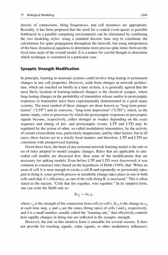
A further innovation in the BCM rule is a nonlinear, essentially parabolic,

relationship between average postsynaptic response and the change in synaptic

weight (Fig. 77.4).

For intermediate to large levels of postsynaptic activity, the effect is like a Reeke

et al. rule with R(+++) and R(�++) both positive, that is, potentiation when activity

is above threshold and depression when activity is below threshold, but here, unlike

the case with the Reeke et al. rule, the amount of depression passes through

a maximum and then declines to zero as postsynaptic activity declines toward

zero. This is probably more realistic, at a cost in increased complexity of

computation.

Synaptic Modification in Spiking ModelsWith spiking models, the simplest approach to synaptic change is to assume it

is slow relative to the firing rate, in which case, the same models that are used with

rate-coded cells can be used – the firing rate needed in the synaptic change rule can

be easily computed from the spike-time data obtained from the spiking model.

However, a great deal of recent experimental evidence shows that, in fact,

changes in synaptic strength are very dependent on the exact timing between pre-

and postsynaptic events. If a presynaptic spike occurs in a limited time interval

before a postsynaptic spike, the synapse is strengthened; conversely, if the presyn-

aptic spike follows the postsynaptic spike, the synapse is likely to be weakened. The

amount of strengthening or weakening decreases as the time between the events

increases (Fig. 77.5).

These data make a great deal of sense: if the presynaptic spike precedes the

postsynaptic one, it may be predictive of that event, and therefore, it might be


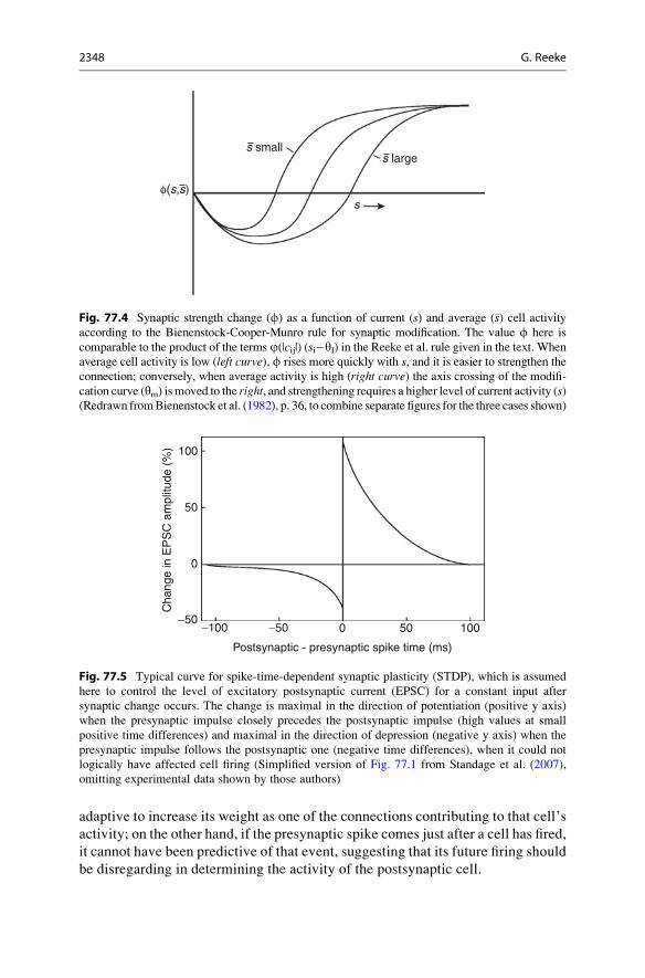
adaptive to increase its weight as one of the connections contributing to that cell’s

activity; on the other hand, if the presynaptic spike comes just after a cell has fired,

it cannot have been predictive of that event, suggesting that its future firing should

be disregarding in determining the activity of the postsynaptic cell.

φ(s,s)

s smalls large

s

Fig. 77.4 Synaptic strength change (f) as a function of current (s) and average (�s) cell activityaccording to the Bienenstock-Cooper-Munro rule for synaptic modification. The value f here is

comparable to the product of the terms j(|cij|) (si�yI) in the Reeke et al. rule given in the text. When

average cell activity is low (left curve), f rises more quickly with s, and it is easier to strengthen theconnection; conversely, when average activity is high (right curve) the axis crossing of the modifi-

cation curve (ym) is moved to the right, and strengthening requires a higher level of current activity (s)(Redrawn fromBienenstock et al. (1982), p. 36, to combine separate figures for the three cases shown)

0

Cha

nge

in E

PS

C a

mpl

itude

(%

) 100

−100 100

50

−5050−50 0

Postsynaptic - presynaptic spike time (ms)

Fig. 77.5 Typical curve for spike-time-dependent synaptic plasticity (STDP), which is assumed

here to control the level of excitatory postsynaptic current (EPSC) for a constant input after

synaptic change occurs. The change is maximal in the direction of potentiation (positive y axis)

when the presynaptic impulse closely precedes the postsynaptic impulse (high values at small

positive time differences) and maximal in the direction of depression (negative y axis) when the

presynaptic impulse follows the postsynaptic one (negative time differences), when it could not

logically have affected cell firing (Simplified version of Fig. 77.1 from Standage et al. (2007),

omitting experimental data shown by those authors)

2348 G. Reeke

The situation is actually more complicated than suggested here, because, except

at low firing rates, a presynaptic spike in fact generally occurs before one postsyn-

aptic spike but after another one; the synaptic modification rule must take into

account the relative timings of all three events. A large number of mathematical

formulations have been proposed for rules consistent with these data and suitable

for use in network simulations. It is beyond the scope of the discussion here to

review these proposals. Anyone interested in modeling synaptic change in networks

of spiking neurons should first become familiar with these proposals and their

relative advantages and disadvantages.

Modeling Tools

A number of free software packages are available for neuronal systems modeling,

and reviews have appeared comparing their features. Some are more suitable for

multicompartment models, others for larger networks of rate-coded cells. All are

based on the same general idea: the differential equations describing cellular

activity and synaptic change are recast as difference equations; the model proceeds

in fixed or variable-length (event-driven) time steps; in each time step, stimuli are

presented; the state variables of each cell and its synapses (or only selected cells in

an event-driven model) are updated according to the specified equations; these new

states are transmitted to all relevant postsynaptic cells, possibly with axonal trans-

mission delays; data are recorded for later analysis or presented in online graphics;

and the process is repeated for as long as desired. In choosing a suitable package,

one should consider not only the types of cell and synaptic models that are available

but also the flexibility in specifying network connectivity, graphics, ease of making

local modifications, and of course, compatibility with available hardware. In the

case of particularly original modeling efforts, it may be necessary to write new

computer code to implement exactly the features that will be needed.

An important aspect of modeling software that should not be overlooked is the

methods that are available for specifying stimuli, their times and sequences of

presentation, sensory modalities affected by those stimuli, and whether the model is

intended to activate effectors that may in turn affect the order of stimulus presen-

tation, as in synthetic neural models. Sensors and effectors may be modeled as part

of an overall system simulation package or may be connected as “plugins” or even

supplied on separate computers via network connections. In the case of robotics

work, sensors and effectors will be real-world devices, for which suitable interfac-

ing software must be provided. This will generally require ad hoc programming

according to the exact types and numbers of devices that need to be interfaced.

While most modeling is today performed on commodity desktop systems, larger

models will usually require some sort of parallel-processing hardware and associated

software to provide adequate performance. This may involve networks of

interconnected standard microprocessors or purpose-built devices based on field

programmable gate arrays (FPGAs) or even custom chips. The widely distributed

neuronal simulation packages generally provide support only for the first of these


alternatives. Recently, it has become possible to program low-cost graphics pro-

cessors on commodity graphics extension boards typically used by computer game

enthusiasts. These provide probably the lowest cost high-performance hardware

available, but programming requires special skills, particularly tomanage the transfer

of data between the main memory and the typically limited graphics card memory.

Nervous System Components Often Omitted from Models

Electrical SynapsesGap junctions and other putative types of electrical synapses have been generally

ignored in neuronal systems modeling up to the present, as they were thought not to

have the plasticity possibilities of chemical synapses. However, experimental data

increasingly indicate the importance of these structures, particularly in areas such as

the inferior olive. Some plasticity may be implemented by changes in the protein

structures implementing the junction. In these situations, the traditional treatment of

gap junctions in models as simple resistive coupling links between compartments on

different cells is inadequate and more sophisticated treatments are beginning to

appear.

Diffusion of Signal MoleculesAnother complication in real nervous systems that is not usually treated in network

models is the diffusion of signal molecules other than neurotransmitters between

cells. This topic became of recognized importance with the discovery of small

signaling molecules such as nitrous oxide and carbon monoxide. Some of these

molecules are capable of diffusing fairly freely across cell membranes, and thus

require a treatment with standard volume diffusion equations rather than standard

synaptic transmission equations. One then needs to model sources of the signal

molecule and their control, for example, synthesis of NO by a Ca2+-dependent

enzyme in postsynaptic cells, decay or active destruction of the signal molecule,

and its effects on target cells, such as modulation of what would otherwise be

Hebbian-like changes in synaptic strength.

Changes in Connectivity, Not Just Connection Strengths: OntogenyThe old doctrine in neuroscience that new neurons are not formed in adult nervous

systems, at least in vertebrates, was overthrown in the 1980s by the discovery of

adult neurogenesis in songbirds and later in mammalian dentate gyrus and other

areas. Improvements in fluorescence labeling and microscope technology have

made it possible to monitor changes in dendritic spines and the presence on them

of synapses in adult neural tissue. Thus, there is ample experimental evidence for

changes not just in synaptic strength, but in synaptic “wiring” that are of interest for

understanding certain disease states in the brain. For example, changes in synaptic

architecture, particularly loss of synapses, are thought to be of particular impor-

tance in schizophrenia and some dementias. These changes are just beginning to

attract attention in the modeling community. A related area of great interest is the

2350 G. Reeke

construction of the nervous system during development, where genetics research is

revealing ever-increasing numbers of signaling molecules that are involved in

directing cell migration and axonal growth, as well as regulating the expression

of other signaling molecules in a coordinated manner. The number of such signals

overwhelms our present ability to understand how they interact to sculpt the

complexity of the adult nervous system. This is an obvious area where more

sophisticated models are likely to be very helpful.

Development of software to handle models of this type is a challenging problem.

Cell migration, neurite growth, and synaptic spine and synapse formation all take

place in three-dimensional space, a feature that is not necessary and therefore not

present in most existing neuronal network models. In these models, a synapse is

represented by a number in a list of connections, and its physical location is

irrelevant; similarly, axonal conduction delays can be represented by numbers in

a data structure without reference to any actual cell locations and axonal structures

connecting them. In order to model growth and recision of structures in three-

dimensional space, each object requires a location, a shape, and a boundary, and the

computer must somehow assure that space is filled without voids or overlaps as

objects expand, change shape, and multiply.

Modeling Tumor GrowthAclosely related area to that of adult neurogenesis is that of tumor growth in the brain.

One would like to be able to model, given imaging data for a specific patient, the

likely future course of the growth of his or her tumor, what critical functional areas

might be affected, where partial resection of the tumor might have the greatest impact

on further growth, what vectors for administration of radiation might cause least

damage to critical structures, and so on. Here one has, perhaps, multiplication of glial

cells rather than of neurons, but the challenges for software development are similar to

those for ontogeny and adult neurogenesis in that a farmore sophisticated treatment of

interacting bodies in three-dimensional space will be required. It will be necessary to

consider the effects of increasing static pressure on neuronal structures and channel

dynamics in the confined space within the skull. One can envision that such models

might involve a combination of techniques from standard neuronal networkmodeling

with techniques from finite-element modeling as used in the engineering disciplines.

Pitfalls

This chapter contains a brief outline of some of the many modeling styles that are

available for studying neuronal systems. If one thing is made clear by this survey, it

is that there is always tension between making a model too abstract, in which case,

properties of the real system that may play important roles in determining behavior

can be overlooked, versus making a model too detailed, in which case, even if it

replicates some observed behavior quite exactly, it may not be possible to tease out

exactly which features are the crucial ones for understanding that behavior. One

should beware of selecting a representation for the neuronal responses or their


changes during learning for reasons of mathematical tractability, because neural

systems are optimized according to criteria imposed by natural selection, not by

computational theory. Thus, it is important in any neuronal modeling exercise to

give careful consideration to this issue, to begin with only those properties that are

found in real nervous systems and that appear to be important in the behavior under

study, but to be prepared to add more detail when the performance of the simplest

model turns out not to approach closely enough to that of the real system.

One should be particularly cautious when incorporating supervised learning into

neuronal models. Not all supervised learning models are alike. While it is certainly

true that humans learn in school under conditions of error correction not unlike

those imposed in supervised learning models, the internal mechanisms are almost

certainly different from the back propagation of errors algorithm that is so often

erroneously implied by the term “supervised learning,” because neuronal systems

lack the circuitry for calculating partial derivatives of outputs with respect to

connection strengths needed with this model as well as the reciprocal connections

needed to transmit individual corrections to individual synapses. Learning mecha-

nisms based on reinforcement learning theory provide a sounder basis for under-

standing learning in neuronal systems. Reinforcement learning still involves an

error signal that is supplied to labile synapses, but now, the error signal is not

tailored to the individual synapse, but rather only provides a global indication of the

adaptive value of recent behavior. This may take the form of internally generated

chemical messages signaling homeostatic state or externally supplied rewards or

punishments in a controlled learning situation. Within this general paradigm, there

is much room for development of new detailed descriptions and models.

In evaluating the success of a model in emulating a particular behavior under

study, it is important that the behavior should actually be produced by the model or

at least be unambiguously signaled by the simulated cells in the model. It is not

always obvious what is the difficult part of a behavior for a nervous system to

produce. In such cases, one might assume that another part of the nervous system,

not included in the model, completes the behavior in question given some input

from the modeled portion. Thus, the model does not actually explain the behavior;

rather, unmodeled other parts of the nervous system are actually critical to the

apparent success of the model. This is a result of overlooking the “homunculus

problem,” the assumption that there is a “little man” or homunculus somewhere in

the brain that completes the work of those parts of a model that were not included,

possibly because they were considered unimportant or trivial. An example of the

homunculus problem might be a model that includes an output cell, the firing of

which is supposed to signal recognition of a familiar face. In this example, suppose

the model recognizes the face from a sample image supplied during training, but the

difficult problem of recognizing a face in different poses at different distances and

from different directions is not included, but rather is left to a homunculus else-

where in the brain. Such a model does little to help us understand how brains

recognize faces.

A converse problem is building in the solution to the problem via construction

of a particular pattern of connectivity or a particular neuronal response function.

2352 G. Reeke

For example, a model of theta oscillation in the hippocampus would be unlikely to

be very informative of how such oscillations are generated and controlled if the cells

in the model were provided with a response function with intrinsic oscillations.

A final point regarding pitfalls in modeling is not to draw strong conclusions

from a run that accidentally works. Many variables in neural models are initialized

or updated by use of random number generators (actually, pseudorandom number

generators). Of course, care should be taken in selecting a random number gener-

ator to pick one that has a sufficiently long repeat cycle for the length of the

contemplated simulations and that also passes well-known tests for independence

of numbers drawn consecutively and at longer separations in the sequence. “Good”

algorithms for random number generation are beyond the scope of this chapter, but

what can be said is that no model should be judged based on a single successful run.

Models should be run with different sequences of pseudorandom numbers (different

“seeds”) and results should also be shown to be robust to changes in numerical

parameters that are fixed during a run, such as numbers of cells, firing thresholds,

ion conductances, decay constants, and so forth.

Outlook

Two ongoing technological developments promise to have a major impact on

neuronal systems modeling studies. One is the increasing number of sensors and

sophistication of analysis software for multielectrode recording; the other is the

ever-increasing power of computing systems – both high-end supercomputers

available at national centers but also commodity computers available to anyone

with a small research budget. The first of these promises more detailed physiolog-

ical data needed to construct realistic models; the second promises the infrastruc-

ture to make the increasingly large models that will be needed to connect low-level

neuronal activity with behavior involving large multi-region brain systems.

Possible modeling developments based on these technologies may include

more models that incorporate three-dimensional neuronal structures and neuronal

systems ontogeny; more attempts to model complete systems, for example, simple

but widely studied lab animals such as the worm Caenorhabditis elegans or the flyDrosophila melanogaster, and more attempts to study very high-level functions,

including even consciousness, in higher vertebrates including humans. It is not

unreasonable to expect that the increasing capabilities of the technical tools will

make it possible for modelers to generate systems sufficiently realistic and sophis-

ticated that collaborations with more conventional experimenters will actually

prove useful to both parties.

Further Reading

Bienenstock EL, Cooper LN, Munro PW (1982) Theory for the development of neuron selectivity:

Orientation specificity and binocular interaction in visual cortex. J Neurosci 2:32


Dayan P, Abbott LF (2001) Theoretical neuroscience: computational and mathematical modeling

of neural systems. MIT Press, Cambridge, MA

Izhikevich EM (2007) Dynamical systems in neuroscience: the geometry of excitability and

bursting. MIT Press, Cambridge, MA

Koch C, Segev I (1998) Methods in neuronal modeling. From ions to networks, 2nd edn. MIT

Press, Cambridge, MA

Krichmar JL, Edelman GM (2008) Design principles and constraints underlying the construction

of brain-based devices. In: Ishikawa M et al (eds) Neural information processing, vol 4985/

2008, Lecture notes in computer science. Springer, Berlin/Heidelberg, pp 157–166.

doi:10.1007/978-3-540-69162-4_17

McCulloch WS, Pitts W (1943) A logical calculus of the ideas immanent in nervous activity. Bull

Math Biophys 5:115

Rieke F, Warland D, de Ruyter van Steveninck R, Bialek W (1997) Spikes: exploring the neural

code. MIT Press, Cambridge, MA

Rosenblatt F (1958) The perceptron: a theory of statistical separability in cognitive systems.

Report no. VG-1196-G-1. Cornell Aeronautical Laboratory, Buffalo, New York

Standage D, Jalil S, Trappenberg T (2007) Computational consequences of experimentally derived

spike-time and weight dependent plasticity rules. Biol Cybern 96:615

Sterratt D, Graham B, Gillies A, Willshaw D (2011) Principles of computational modelling in

neuroscience. Cambridge University Press, Cambridge/New York

Sutton RS, Barto AG (1998) Reinforcement learning: an introduction. MIT Press, Cambridge, MA

Traub RD, Miles R (1991) Neuronal networks of the Hippocampus. Cambridge University Press,

Cambridge

2354 G. Reeke

Documents

Neuroscience in the 21st Century || Biological Modeling