Embed Size (px)
Citation preview
Neuromodulation of
Peripheral Nerve Excitability
Using Ultrasound
by
Sanchit Chirania
A Thesis Presented in Partial Fulfillment of the Requirements for the Degree
Master of Science
Approved November 2016 by the Graduate Supervisory Committee:
Bruce Towe, Chair
James Abbas Jitendran Muthuswamy
ARIZONA STATE UNIVERSITY
December 2016
i
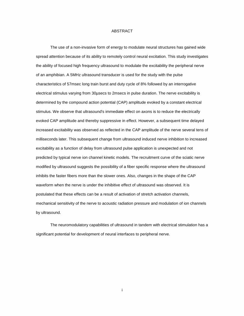
ABSTRACT
The use of a non-invasive form of energy to modulate neural structures has gained wide
spread attention because of its ability to remotely control neural excitation. This study investigates
the ability of focused high frequency ultrasound to modulate the excitability the peripheral nerve
of an amphibian. A 5MHz ultrasound transducer is used for the study with the pulse
characteristics of 57msec long train burst and duty cycle of 8% followed by an interrogative
electrical stimulus varying from 30µsecs to 2msecs in pulse duration. The nerve excitability is
determined by the compound action potential (CAP) amplitude evoked by a constant electrical
stimulus. We observe that ultrasound's immediate effect on axons is to reduce the electrically
evoked CAP amplitude and thereby suppressive in effect. However, a subsequent time delayed
increased excitability was observed as reflected in the CAP amplitude of the nerve several tens of
milliseconds later. This subsequent change from ultrasound induced nerve inhibition to increased
excitability as a function of delay from ultrasound pulse application is unexpected and not
predicted by typical nerve ion channel kinetic models. The recruitment curve of the sciatic nerve
modified by ultrasound suggests the possibility of a fiber specific response where the ultrasound
inhibits the faster fibers more than the slower ones. Also, changes in the shape of the CAP
waveform when the nerve is under the inhibitive effect of ultrasound was observed. It is
postulated that these effects can be a result of activation of stretch activation channels,
mechanical sensitivity of the nerve to acoustic radiation pressure and modulation of ion channels
by ultrasound.
The neuromodulatory capabilities of ultrasound in tandem with electrical stimulation has a
significant potential for development of neural interfaces to peripheral nerve.

ii
DEDICATION
I dedicate this work to my parents, Satish Chirania and Madhu Chirania and my lovely
sister Aayushi Chirania for their undying support, selfless love and constant motivation. You have
taught me one of the most important virtue of life: Patience. Words are not enough to describe the
sacrifices you’ve made and I owe all of my success now and in the future to you.
Also, my role model: Late Dr. A.P.J Abdul Kalam, former President of India. You have
been my inspiration since childhood and your belief that science should be applied for the greater
good of mankind has driven me to choose science as my career. “You have to dream before your
dreams can come true” – this quote from you will always resonate in all my actions.
iii
ACKNOWLEDGMENTS
I would like to sincerely thank Dr. Bruce Towe, who has served as my principal
investigator and for giving me this opportunity to pursue research and culminate my Master's
experience with a thesis. He has been very motivating, enthusiastic and patient with my questions
throughout the course of my thesis work. And for staying back in the lab till several midnights to
help with my experiments. He is very passionate when it comes to science and I have acquired
some amazing skills working under his guidance.
I want to thank Dr. Jitendran Muthuswamy and Dr. James Abbas for investing their time
in being a part of my defense committee and for their valuable suggestions. Time and again, their
support has made this long journey look very easy. I would also like to thank Dr. Richard Herman
for his constant guidance and pushing me to work, take more data sets that has helped in
culminating a detailed work of my thesis.
Special thanks to Yashwanth Nanda Kumar, Swarnima Pandey & Ranjani Sampath
Kumaran for helping balance my entrepreneurial and master’s life.
Finally, and most importantly, my friends and colleagues who have been a pillar of
support, encouraging me at every single step and for cheering me up every time I encountered a
failure. You are my family here at Arizona.
Thanks a lot: Sneha Shenoy, Nathaniel Bennett, Sivakumar Palaniswamy, Krishan Sharma,
Saveetha Raghunathan, Prabath Vemullapalli, Madhusudhanan Parthasarthy and Sanal Parakat
and the list goes on!!
iv
TABLE OF CONTENTS
Page
LIST OF TABLES ................................................................................................................................... vi
LIST OF FIGURES ................................................................................................................................ vii
CHAPTER
1 INTRODUCTION ................. ................................................................................................... 1
2 BACKGROUND ................... ................................................................................................... 3
2.1 Frog Sciatic Nerve Anantomy ........................................................................ 3
2.2 Nerve Conduction ........................................................................................... 4
2.3 Ultrasound ....................................................................................................... 8
2.4 Literature Survey .......................................................................................... 10
3 METHODS ...................... ...................................................................................................... 13
3.1 Bullfrog Sciatic Nerve extraction .................................................................. 13
3.2 Focused Ultrasound Transducer.................................................................. 14
3.3 Experimental Setup ...................................................................................... 17
4 RESULTS ...................... ....................................................................................................... 22
4.1 Compound Action Potential .......................................................................... 22
4.2 Suppression of CAP with Ultrasound........................................................... 22
4.3 Latency Effect of Ultrasound ........................................................................ 26
4.4 Effect of Ultrasound on Strength-Duration Curve ........................................ 32
4.5 Morphology Changes in CAP ....................................................................... 34
5 DISCUSSION....................... .................................................................................................. 36
5.1 Suppression of Compound Action Potential (CAP) ..................................... 36
5.2 Recruitment Curve ........................................................................................ 37
5.3 The Overshoot Followed After Inhibition ..................................................... 37
5.4 Chronaxie Shift ............................................................................................. 40
5.5 Morphology Change ..................................................................................... 40
v
6 CONCLUSION ....................... ............................................................................................... 41
REFERENCES....... ............................................................................................................................ 43
APPENDIX
A ULTRASOUND LATENCY EFFECT DATA SETS................. ............................................. 45
vi
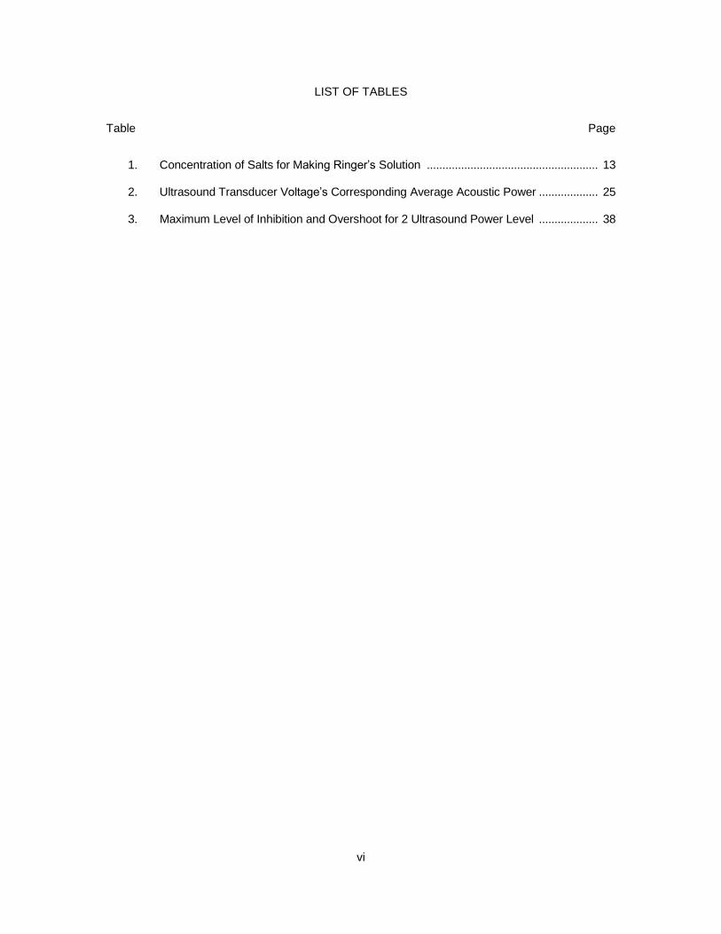
LIST OF TABLES
Table Page
1. Concentration of Salts for Making Ringer’s Solution ....................................................... 13
2. Ultrasound Transducer Voltage’s Corresponding Average Acoustic Power ................... 25
3. Maximum Level of Inhibition and Overshoot for 2 Ultrasound Power Level ................... 38
vii
LIST OF FIGURES
Figure Page
1. Schematic Diagram of Sciatic Nerve in Frog ................................................................... 3
2. Conduction Velocity Plotted Versus Fiber Diameter for Sciatic Nerve of a Bullfrog ...... 4
3. The Different Stages of Action Potential .......................................................................... 6
4. Strength-Duration Curve by Lapicque .............................................................................. 8
5. Reverse Piezoelectric Effect to Produce Ultrasound ....................................................... 9
6. Unfocused and Focused Ultrasound Transducer ............................................................ 9
7. Percent Amplitude Change for CAP Peaks as a Function of Ispta ............................... 12
8. Force Balance Test to Measure Acoustic Power of 5Mhz Transducer ........................ 16
9. Schematic Diagram of the Setup ................................................................................... 17
10. Expermimental Setup Overview ...................................................................................... 18
11. Pulse Characteristics ...................................................................................................... 18
12. Nerve Bath with Ultrasound Transducer Fixed in the Bottom, Nerve Suspended in Ringer’s
With the Help of Stimulating and Recording Electrode on the Other End .................... 19
13. Sciatic Nerve Suspended in Ringer’s Solution With Two Stimulating Silver Silver Chloride
Hook Electrode ................................................................................................................ 20
14. Recording Silver Silver Chloride Electrodes .................................................................. 21
15. Compound Action Potential (CAP) Recorded ................................................................ 22
16. Graph Showing Suppression in Amplitude of CAP Because of Ultrasound Exposure. 50%
CAP is Also Shown as a Comparison ............................................................................ 23
17. CAP Peak to Peak Amplitude Versus Ultrasound Drive Voltage for In Focus and Out Of
Focus Nerve Target ........................................................................................................ 24
18. CAP as a Percentage of Saturated Value (100%) Starting With an Electrical Stimulus at
50% Versus Ultrasound Drive Voltage for In Focus and Out Of Focus Nerve Target .. 24
19. Nerve Recruitment Curve Plotted With CAP Peak to Peak Amplitude Versus Electrical
Stimulation Voltage .......................................................................................................... 26
viii
Figure Page
20. Nerve Recruitment Curve Plotted With Percentage of Nerve Fiber Recruitment Versus
Electrical Stimulation Voltage .......................................................................................... 26
21. 50% CAP After Exposure to Ultrasound is Suppressed Immediately Followed by
Enhancement Few Tens of Msecs Later ........................................................................ 27
22. CAP Peak to Peak Amplitude as Processed by Labview .............................................. 28
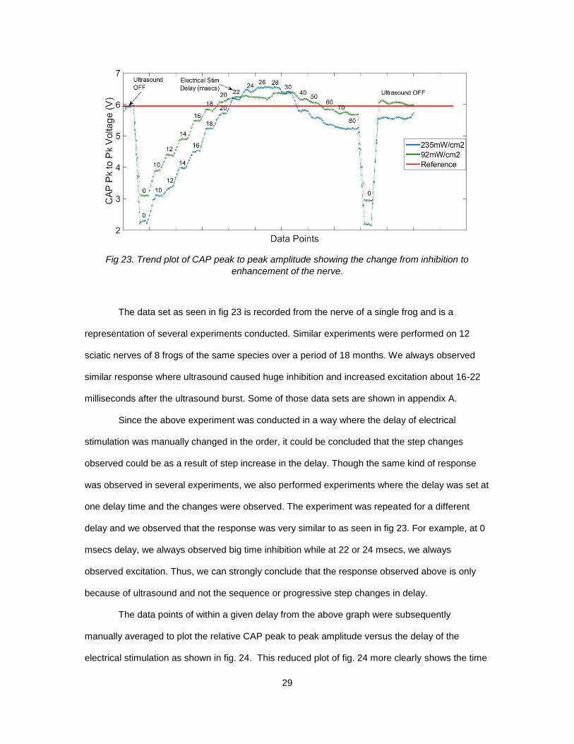
23. Trend Plot of CAP Peak to Peak Amplitude Showing the Change From Inhibition to
Enhancement of the Nerve .............................................................................................. 29
24. Averaged Trend Plot of CAP Peak to Peak Amplitude Versus the Delay of Electrical
Stimulation ...................................................................................................................... 30
25. Recruitment of Nerve in % Versus Delay of Electrical Stimulus ................................... 31
26. Suppression of CAP in % Versus Electrial Stimulation Delay........................................ 31
27. Strength-Duration Curve of Frog Sciatic Nerve With and Without Ultrasound Exposure 33
28. Close Up View of Lower Pulse Width Part of the Strength-Duration Curve ................. 33
29. Morphology Changes in CAP Waveform ........................................................................ 35
30. Trend Plot of CAP Peak to Peak Voltage as the Delay of Electrical Stimulation is Varied for
Ultrasound Power Level of 235mW/cm2 ......................................................................... 46
31. Trend Plot of CAP Peak to Peak Voltage as the Delay of Electrical Stimulation is Coarsely
Varied for Ultrasound Power Level of 120mW/cm2 ........................................................ 46
32. Trend Plot of CAP Peak to Peak Voltage as the Delay of Electrical Stimulation is Varied for
Ultrasound Power Level of 120mW/cm2. The Data Recording Stopped at 30msec ..... 47
33. Trend Plot of CAP Peak to Peak Voltage as the Delay of Electrical Stimulation is Varied for
Ultrasound Power Level of 120mW/cm2 ......................................................................... 47
34. Trend Plot of CAP Peak to Peak Voltage as the Delay of Electrical Stimulation is Varied for
Ultrasound Power Level of 80mW/cm2 ........................................................................... 48
1
CHAPTER 1
INTRODUCTION
The word “Neuromodulation” as defined by the International Neuromodulation society:
“the alteration of nerve activity through the delivery of electrical stimulation or chemical agents to
targeted sites of the body” [1]. In simple terms, a device (neurostimulators) or procedure having
an ability to change/modulate the behaviour of a nerve. Most of the neurostimulators used today
including pacemakers and spinal cord stimulators use electric signals to modulate the activity of
nerves and require invasive procedures for placement inside of a human body. The demanding
invasive procedures gave birth to the idea of having simple yet effective non-invasive methods.
For the past few decades, researchers have worked on developing non-invasive
neuromodulation techniques and one of them is high frequency (in MHz range) acoustic wave or
ultrasound based neuromodulation. Ultrasound based diagnostic imaging has been a mainstay in
the medical imaging market for decades because of its ability to penetrate deeper tissues.
Utilizing the same feature, ultrasound can be very useful for neuromodulation both in central
nervous system (CNS) and peripheral nervous system (PNS).
In PNS, focused and pulsed high frequency ultrasound can alter the functioning of the
peripheral nerves. There has been several research done in the past on usage of ultrasound for
neuromodulation of peripheral nerves. Some of them were focused on investigation of effects of
high-intensity focused ultrasound (HIFU) on in-vitro peripheral nerve model [2]–[7]. The initial
findings from these research suggest that HIFU can both enhance and suppress the neural
conduction activity of the nerve based on the acoustic power. Most of them had relatively longer
duration of ultrasound exposure and the effects lasted for seconds in some cases.
The holy grail behind the idea of neuromodulation of peripheral nervous system is the
ability to modulate the nerve conduction activity at will i.e. be able to excite and inhibit the nerve
with the same setup as and when required. Keeping this mind, the idea of this study is to
understand the response of a nerve when exposed to ultrasound and develop a system where in
a focused ultrasound can be used as an alternative or adjunct to electrical stimulation for

2
modulating the nerve. This study is focused on understanding the neuromodulatory effects of
comparatively low duration exposure of focused and pulsed high frequency ultrasound of 5 Mhz.
3
CHAPTER 2
BACKGROUND
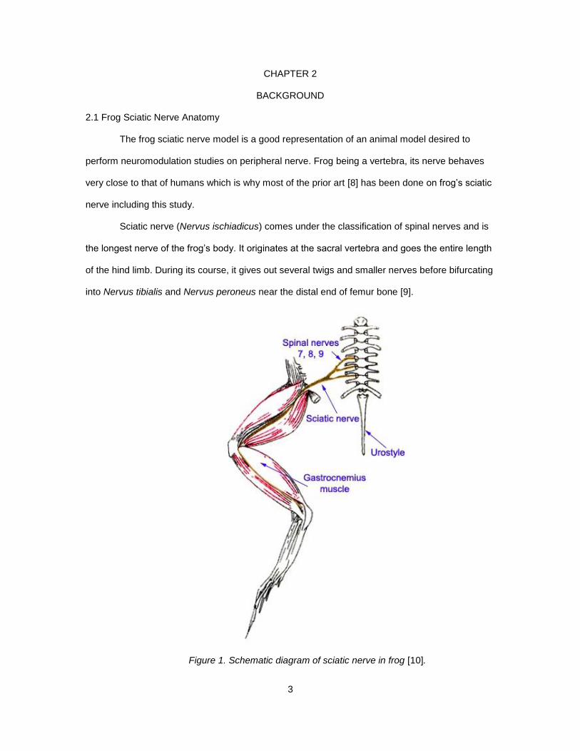
2.1 Frog Sciatic Nerve Anatomy
The frog sciatic nerve model is a good representation of an animal model desired to
perform neuromodulation studies on peripheral nerve. Frog being a vertebra, its nerve behaves
very close to that of humans which is why most of the prior art [8] has been done on frog’s sciatic
nerve including this study.
Sciatic nerve (Nervus ischiadicus) comes under the classification of spinal nerves and is
the longest nerve of the frog’s body. It originates at the sacral vertebra and goes the entire length
of the hind limb. During its course, it gives out several twigs and smaller nerves before bifurcating
into Nervus tibialis and Nervus peroneus near the distal end of femur bone [9].
Figure 1. Schematic diagram of sciatic nerve in frog [10].
4
2.2 Nerve Conduction
2.2.1 Conduction studies and Compound Action Potential
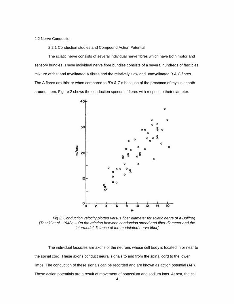
The sciatic nerve consists of several individual nerve fibres which have both motor and
sensory bundles. These individual nerve fibre bundles consists of a several hundreds of fascicles,
mixture of fast and myelinated A fibres and the relatively slow and unmyelinated B & C fibres.
The A fibres are thicker when compared to B’s & C’s because of the presence of myelin sheath
around them. Figure 2 shows the conduction speeds of fibres with respect to their diameter.
Fig 2. Conduction velocity plotted versus fiber diameter for sciatic nerve of a Bullfrog
[Tasaki et al., 1943a – On the relation between conduction speed and fiber diameter and the
intermodal distance of the modulated nerve fiber]
The individual fascicles are axons of the neurons whose cell body is located in or near to
the spinal cord. These axons conduct neural signals to and from the spinal cord to the lower
limbs. The conduction of these signals can be recorded and are known as action potential (AP).
These action potentials are a result of movement of potassium and sodium ions. At rest, the cell
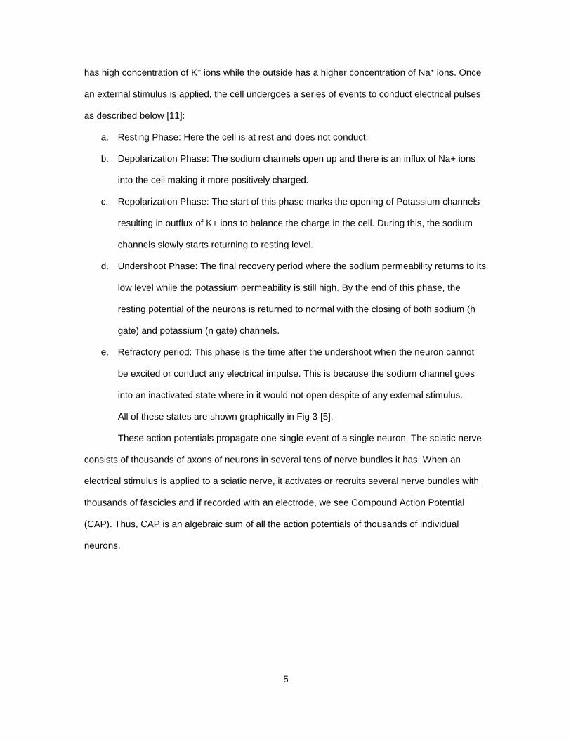
5
has high concentration of K+ ions while the outside has a higher concentration of Na+ ions. Once
an external stimulus is applied, the cell undergoes a series of events to conduct electrical pulses
as described below [11]:
a. Resting Phase: Here the cell is at rest and does not conduct.
b. Depolarization Phase: The sodium channels open up and there is an influx of Na+ ions
into the cell making it more positively charged.
c. Repolarization Phase: The start of this phase marks the opening of Potassium channels
resulting in outflux of K+ ions to balance the charge in the cell. During this, the sodium
channels slowly starts returning to resting level.
d. Undershoot Phase: The final recovery period where the sodium permeability returns to its
low level while the potassium permeability is still high. By the end of this phase, the
resting potential of the neurons is returned to normal with the closing of both sodium (h
gate) and potassium (n gate) channels.
e. Refractory period: This phase is the time after the undershoot when the neuron cannot
be excited or conduct any electrical impulse. This is because the sodium channel goes
into an inactivated state where in it would not open despite of any external stimulus.
All of these states are shown graphically in Fig 3 [5].
These action potentials propagate one single event of a single neuron. The sciatic nerve
consists of thousands of axons of neurons in several tens of nerve bundles it has. When an
electrical stimulus is applied to a sciatic nerve, it activates or recruits several nerve bundles with
thousands of fascicles and if recorded with an electrode, we see Compound Action Potential
(CAP). Thus, CAP is an algebraic sum of all the action potentials of thousands of individual
neurons.
6
Fig 3. The different stages of action potential [11]. [a] Resting stage. [b] Depolarization.
[c] Repolarization. [d] Undershoot.
7
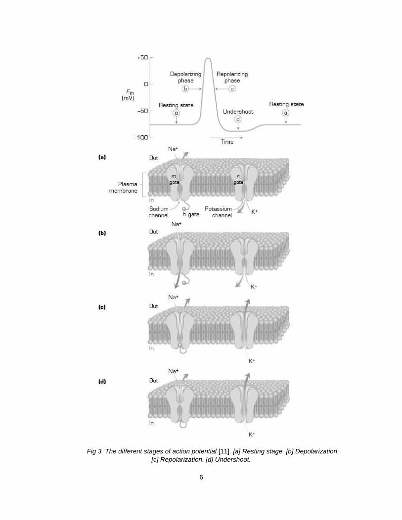
2.2.2 Rheobase and Chronaxie
Near the end of the 19th century, researchers were working on developing a
mathematical relationship describing the phenomenon of electrical stimulation. It was very
important to understand the threshold of excitation for a given pulse. This will provide useful
insight into the amount of electricity required to be deposited for a successful electrostimulation of
biological tissues which varies from species to species.
One of the first attempt was by Georges Weiss who reported that the relationship
between duration of pulse and the applied electrical voltage is linear [12]. Although it was
convenient to assume the linear relationship, it could not be applied to every biological nerves or
muscles model. Several experiments conducted showed a more hyperbolic response as shown
by Lapicque [13]. After carefully studying various biological system, he came up with the following
formula:
Stimulus Intensity = Rheobase * (1 + Chronaxie/Pulse Duration) [14]
where, Rheobase = minimum intensity with long duration to reach threshold
Chronaxie = characteristic duration at which a current of double Rheobase is flowing
The above equation can be represented as a Strength-Duration curve for rectangular
pulse is shown in Fig 4. Rheobase contains two most important information: firstly, it defines the
threshold voltage that is essentially required to stimulate the biological system when the
rectangular pulse duration is considered long or infinite. And secondly, it defines the safety
standard for stimulation i.e. the maximum voltage that can be applied and still not stimulate the
biological system.
Chronaxie on the other hand, is defined as the pulse duration required to achieve twice
the Rheobase voltage. The chronaxie plays a similar role in a hyperbola as the time constant in
an exponential function; it determines how fast the strength-duration curve approaches its final
value. Chronaxie is a characteristic for excitability of biological system which is modified or
changed by physical and physiological parameters [14]. Also, chronaxie is considered as the
optimum pulse duration time that can safely stimulate with minimum electrical energy deposited.
Thus, it not only gives out important information on the pulse duration for a particular biological
8
system, but also looking for changes in the Chronaxie tells that the physiological parameter has
changed. This is very important with respect to this study as we are looking for neuromodulation
of peripheral nerves using ultrasound.
Fig 4. Strength-duration curve by Lapicque. The threshold expressed as intensity I
(voltage or current) applied is a hyperbolic function of the pulse duration t. Source: [15]
2.3 Ultrasound
Ultrasound as defined by the American National Standards Institute is the sound
frequencies which are greater than 20 kHz which is well above the audible hearing limit of
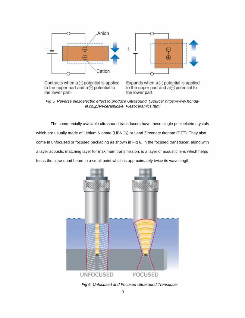
humans. Ultrasound can be produced by the reverse piezoelectric phenomenon wherein when a
voltage is applied across a piezoelectric material, the distance between atoms in crystal lattice
changes slightly deforming the crystal. This deformation in the crystal causes the material to
vibrate rapidly (depends upon the applied frequency of electrical signal) producing sound waves
called Ultrasound. Fig 5. shows the reverse piezoelectric effect.
9
Fig 5. Reverse piezoelectric effect to produce Ultrasound. (Source: https://www.honda-
el.co.jp/en/ceramics/e_Piezoceramics.html
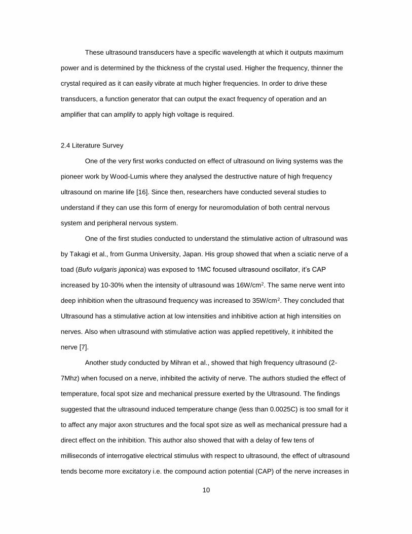
The commercially available ultrasound transducers have these single peizoelctric crystals
which are usually made of Lithium Niobate (LiBNO3) or Lead Zirconate titanate (PZT). They also
come in unfocused or focused packaging as shown in Fig 6. In the focused transducer, along with
a layer acoustic matching layer for maximum transmission, is a layer of acoustic lens which helps
focus the ultrasound beam to a small point which is approximately twice its wavelength.
Fig 6. Unfocused and Focused Ultrasound Transducer
10
These ultrasound transducers have a specific wavelength at which it outputs maximum
power and is determined by the thickness of the crystal used. Higher the frequency, thinner the
crystal required as it can easily vibrate at much higher frequencies. In order to drive these
transducers, a function generator that can output the exact frequency of operation and an
amplifier that can amplify to apply high voltage is required.
2.4 Literature Survey
One of the very first works conducted on effect of ultrasound on living systems was the
pioneer work by Wood-Lumis where they analysed the destructive nature of high frequency
ultrasound on marine life [16]. Since then, researchers have conducted several studies to
understand if they can use this form of energy for neuromodulation of both central nervous
system and peripheral nervous system.
One of the first studies conducted to understand the stimulative action of ultrasound was
by Takagi et al., from Gunma University, Japan. His group showed that when a sciatic nerve of a
toad (Bufo vulgaris japonica) was exposed to 1MC focused ultrasound oscillator, it’s CAP
increased by 10-30% when the intensity of ultrasound was 16W/cm2. The same nerve went into
deep inhibition when the ultrasound frequency was increased to 35W/cm2. They concluded that
Ultrasound has a stimulative action at low intensities and inhibitive action at high intensities on
nerves. Also when ultrasound with stimulative action was applied repetitively, it inhibited the
nerve [7].
Another study conducted by Mihran et al., showed that high frequency ultrasound (2-
7Mhz) when focused on a nerve, inhibited the activity of nerve. The authors studied the effect of
temperature, focal spot size and mechanical pressure exerted by the Ultrasound. The findings
suggested that the ultrasound induced temperature change (less than 0.0025C) is too small for it
to affect any major axon structures and the focal spot size as well as mechanical pressure had a
direct effect on the inhibition. This author also showed that with a delay of few tens of
milliseconds of interrogative electrical stimulus with respect to ultrasound, the effect of ultrasound
tends become more excitatory i.e. the compound action potential (CAP) of the nerve increases in
11
amplitude for the same electrical pulse. Thus, they showed both enhancement and suppression
of the nerve can be obtained and that the effect of ultrasound is reversible [4].
Similar experiments were carried out by Phillips et al., where frog sciatic nerve was
exposed relatively higher ultrasound frequency of 17.5MHz. The study focused on understanding
the long term exposure of tone bursts of ultrasound at 10Hz, 20ms pulse widths with 20 seconds
duration at power levels ~25-150W/cm2 Itp. Large ultrasound-initiated enhancement of CAP was
seen routinely but deep value of suppression appeared less frequently. The author concluded the
effect as a result of combination of thermal heating and mechanical (radiation force) induced
effects of ultrasound [5].
Colucci et al., studied the effects of long term exposure to Ultrasound. He found that
when frog’s sciatic nerve was exposed to 30 second sonication of a focused ultrasound
transducer of 0.661 MHz at 16W (equivalent to 440W/cm2), there was complete nerve conduction
block. It took about 90 minutes for the nerve to recover completely from the block. In cases of
higher intensity (650W/cm2), the nerve completely lost its CAP and did not recover at all. With the
help of a thermocouple, it was observed that there was a significant increase in the temperature
on the nerve which resulted in a block. Another experiment conducted by heating the Ringer’s
solution gave the same result as that of high intensity ultrasound confirming that the suppression
of the nerve by ultrasound was due to thermal effects [2].
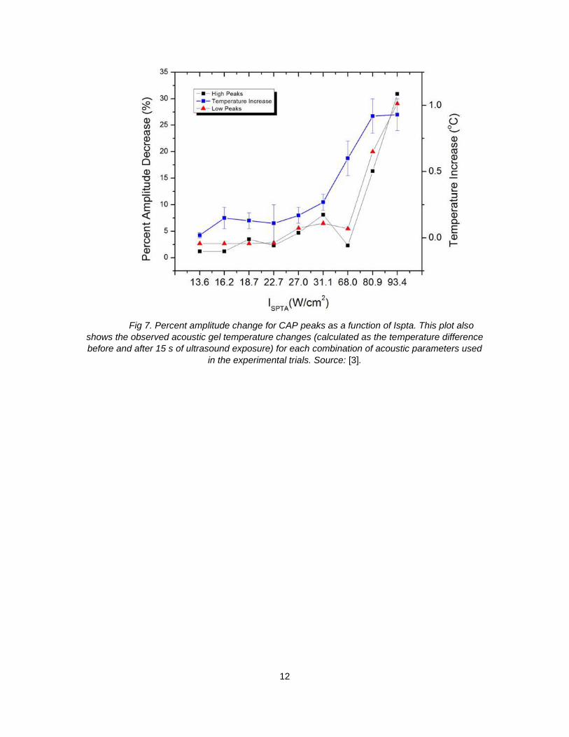
All of the above conducted experiments were in vitro studies Juan et al., conducted in
vivo studies on the vagus nerve of Long evans rats. They found that when the nerve was
exposed to 15 seconds of 1.1 MHz focused ultrasound, it inhibited the nerve to almost 30% with a
temperature rise of about 1ºC as shown in fig 7. The authors analysed that with the exposure to
ultrasound not only the evoked potentials decreased, so did the conduction velocity. This is in
contradiction with literature reports showing with increase in temperature, the conduction velocity
of peripheral nerves increases [17]. Thus, the conclusion that it is not the temperature alone that
contributes to the inhibition of the nerve but also the mechanical pressure wave of ultrasound that
can cause inhibition[3].
12
Fig 7. Percent amplitude change for CAP peaks as a function of Ispta. This plot also
shows the observed acoustic gel temperature changes (calculated as the temperature difference
before and after 15 s of ultrasound exposure) for each combination of acoustic parameters used
in the experimental trials. Source: [3].
13
CHAPTER 3
METHODS
3.1 Bullfrog Sciatic Nerve extraction
This was an in vitro study conducted on sciatic nerve of an American Bullfrog (Lithobates
catesbeiana) and required excising the nerve to conduct experiments for detecting changes in the
nerve threshold response. The advantage of using frogs is the simplicity in dissection and ease in
maintaining the excised nerve. Unlike rats, the amphibian’s nerve only needs to be constantly
immersed in Ringer’s solution and can last almost 8-10 hours and does not necessarily need
constant oxygen supply with temperature maintenance.
3.1.1 Ringer’s Solution
While the frog is being dissected, it is important to continuously wet it in Ringer’s
solution so that the cells don’t dry up. The excised nerve always needs to be kept moist with a
constant supply of glucose to make sure the axons of the cells are alive. Ringer’s solution is a
mixture of various salts in water that creates an isotonic solution replicating the internal
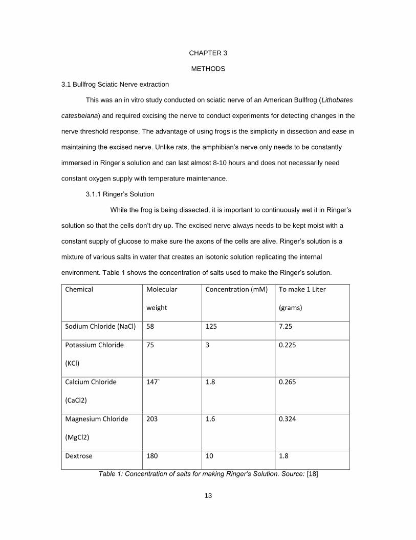
environment. Table 1 shows the concentration of salts used to make the Ringer’s solution.
Chemical Molecular
weight
Concentration (mM) To make 1 Liter
(grams)
Sodium Chloride (NaCl) 58 125 7.25
Potassium Chloride
(KCl)
75 3 0.225
Calcium Chloride
(CaCl2)
147` 1.8 0.265
Magnesium Chloride
(MgCl2)
203 1.6 0.324
Dextrose 180 10 1.8
Table 1: Concentration of salts for making Ringer’s Solution. Source: [18]
14
3.1.2 Dissection
The experiments on American Bullfrog protocol (#16-1476R) was approved by
Institutional Animal Care and Use Committee (IACUC), Office of Research Integrity and
Assurance, Arizona State University. The bullfrogs used in the experiments ranged from 8 to 12
inches in length from snout to fin.
Bullfrog is first placed in a shallow bath of 0.2% Tricaine ethanesulfonate (MS-222)
(C9H11NO2.CH4SO3) solution for 20 minutes. The bath puts the animal in a state of anaesthesia.
The correct level of anaesthesia is verified by tipping the frog sideways; if the frog attempts to
remain upright, it is not ready and must remain longer in the bath. When the animal is sufficiently
anesthetized, a heavy scissor is positioned caudal to the eyes, and with a single coronal incision
the animal is euthanized. The incision exposes the spinal cord, and a blunt probe is stirred within
the spinal canal to ensure complete decerebration. Thus the animal is not alive during the rest of
the experiment.
After the decerebration, frog is then flipped and the sciatic nerve dissection is started in
one of the legs. BY locating the sciatic nerve near the femur bone, it is followed till the sesamoid
bone and released from the muscles around it. The nerve is then followed all the way up to the
spinal cord. The distal end of the nerve is severed and pulled out of its leg and then it is cut from
the spinal cord. The extracted nerve is immediately transferred in a fresh isotonic ringer’s
solution. The sciatic nerve of the other leg is also extracted and stored in a petri dish with
Ringer’s solution at room temperature. The excised nerves were usually 3-5inches in length with
a diameter of 1-1.5mm.
3.2 Focused Ultrasound Transducer
For the purpose of this study, a half inch diameter element, focused Ultrasound
transducer from Valpey Fischer was used with fundamental frequency of 5MHz. It had a half-inch
piezo crystal as its element.
3.2.1 Focal distance and focal spot size calculation
15
To calculate the focal distance of the transducer experimentally, we used the
concept of cavitation. When the surface of the water is exactly at the focal point of the transducer,
it cavitates and water is thrown up in thin jet. And the thickness of the water jet tells the
approximate focal spot size of the transducer. These values are critical as they will help decide
the required distance of the nerve from the transducer and in calculation of the power of
ultrasound.
The transducer was fitted inside a 12ml syringe from one end and the other end was cut.
Water was filled to about 1 inch from the surface of transducer and the setup was made
stationary by attaching it to a holder. Ultrasound transducer was then excited with a tone burst at
5MHz and water slowly added using a pipette. When the water level reached about 2inches, the
water was thrown in a jet stream to about 12 inches from the surface and heavy cavitation was
observed. Also the diameter of the water jet was about 2mm.
The focal distance was thus confirmed to be 2inches and focal spot size as 2mm.
3.2.2 Ultrasound Acoustic Power test
FDA regulates the acoustic power that can be used on a clinical system. As per
the FDA limits, the average peak power of an acoustic wave applied to humans should not
exceed 720 mW/cm2. This value can be derived with the help of a simple force balance
experiment.
The acoustic power was measured by the setup in the figure 8. The 5MHz ultrasound
transducer is connected to a function generator through an Ophir amplifier. It is then operated
using a tone burst on the same settings as used in this study. The pulse characteristics is as
described in fig 11. The transducer is suspended in a distilled water column with a highly acoustic
wave absorptive material like silicone. The whole setup is mounted on a weighing scale (Mettler
AE240 with a sensitivity of 0.1g). Whole setup is left undisturbed overnight.
The following day the transducer was powered by the linear power amplifier and the
change in mass was recorded. The equation below is used to determine the acoustic power [19].
16
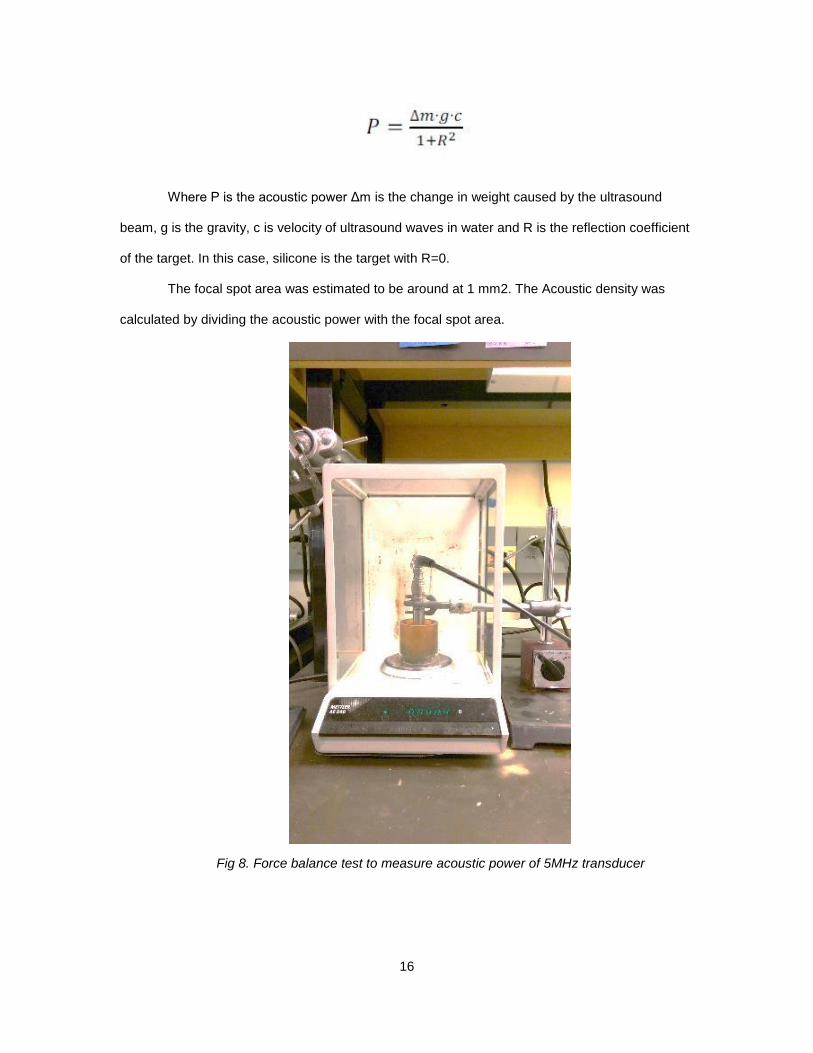
Where P is the acoustic power Δm is the change in weight caused by the ultrasound
beam, g is the gravity, c is velocity of ultrasound waves in water and R is the reflection coefficient
of the target. In this case, silicone is the target with R=0.
The focal spot area was estimated to be around at 1 mm2. The Acoustic density was
calculated by dividing the acoustic power with the focal spot area.
Fig 8. Force balance test to measure acoustic power of 5MHz transducer
17
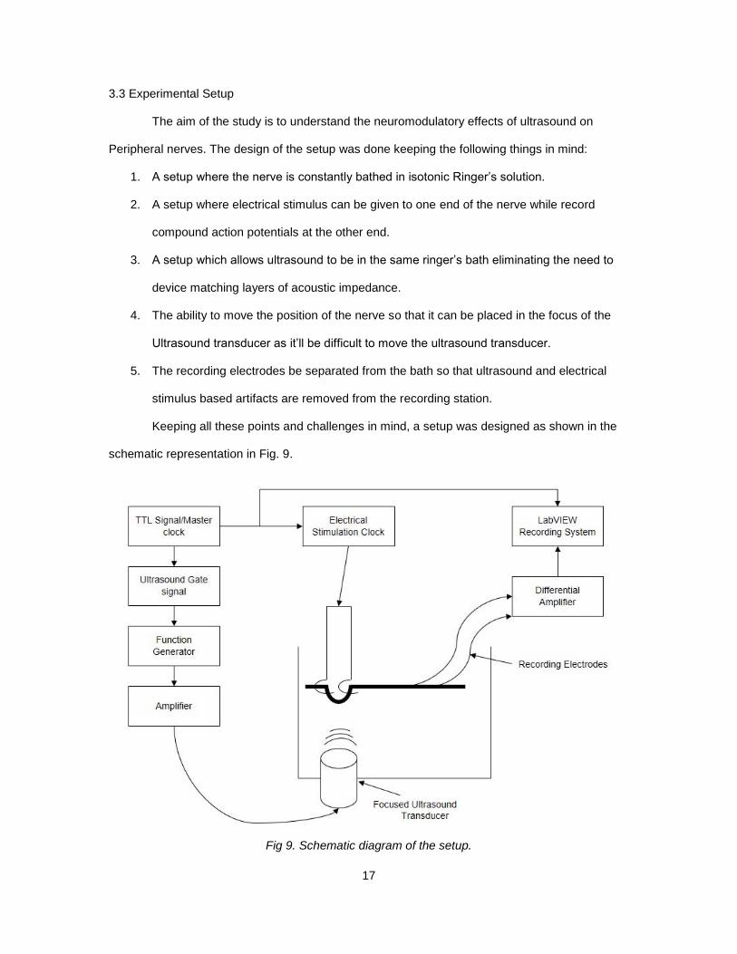
3.3 Experimental Setup
The aim of the study is to understand the neuromodulatory effects of ultrasound on
Peripheral nerves. The design of the setup was done keeping the following things in mind:
1. A setup where the nerve is constantly bathed in isotonic Ringer’s solution.
2. A setup where electrical stimulus can be given to one end of the nerve while record
compound action potentials at the other end.
3. A setup which allows ultrasound to be in the same ringer’s bath eliminating the need to
device matching layers of acoustic impedance.
4. The ability to move the position of the nerve so that it can be placed in the focus of the
Ultrasound transducer as it’ll be difficult to move the ultrasound transducer.
5. The recording electrodes be separated from the bath so that ultrasound and electrical
stimulus based artifacts are removed from the recording station.
Keeping all these points and challenges in mind, a setup was designed as shown in the
schematic representation in Fig. 9.
Fig 9. Schematic diagram of the setup.
18
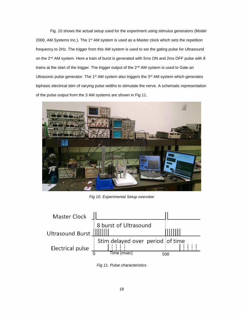
Fig. 10 shows the actual setup used for the experiment using stimulus generators (Model
2000, AM Systems Inc.). The 1st AM system is used as a Master clock which sets the repetition
frequency to 2Hz. The trigger from this AM system is used to set the gating pulse for Ultrasound
on the 2nd AM system. Here a train of burst is generated with 5ms ON and 2ms OFF pulse with 8
trains at the start of the trigger. The trigger output of the 2nd AM system is used to Gate an
Ultrasonic pulse generator. The 1st AM system also triggers the 3rd AM system which generates
biphasic electrical stim of varying pulse widths to stimulate the nerve. A schematic representation
of the pulse output from the 3 AM systems are shown in Fig 11.
Fig 10. Experimental Setup overview
Fig 11. Pulse characteristics
19
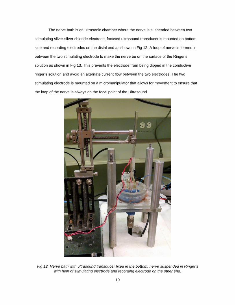
The nerve bath is an ultrasonic chamber where the nerve is suspended between two
stimulating silver-silver chloride electrode, focused ultrasound transducer is mounted on bottom
side and recording electrodes on the distal end as shown in Fig 12. A loop of nerve is formed in
between the two stimulating electrode to make the nerve be on the surface of the Ringer’s
solution as shown in Fig 13. This prevents the electrode from being dipped in the conductive
ringer’s solution and avoid an alternate current flow between the two electrodes. The two
stimulating electrode is mounted on a micromanipulator that allows for movement to ensure that
the loop of the nerve is always on the focal point of the Ultrasound.
Fig 12. Nerve bath with ultrasound transducer fixed in the bottom, nerve suspended in Ringer’s
with help of stimulating electrode and recording electrode on the other end.
20
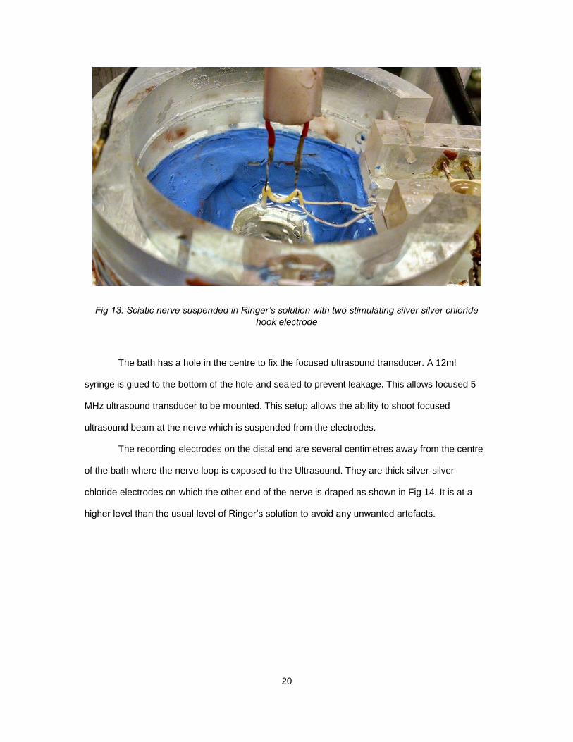
Fig 13. Sciatic nerve suspended in Ringer’s solution with two stimulating silver silver chloride
hook electrode
The bath has a hole in the centre to fix the focused ultrasound transducer. A 12ml
syringe is glued to the bottom of the hole and sealed to prevent leakage. This allows focused 5
MHz ultrasound transducer to be mounted. This setup allows the ability to shoot focused
ultrasound beam at the nerve which is suspended from the electrodes.
The recording electrodes on the distal end are several centimetres away from the centre
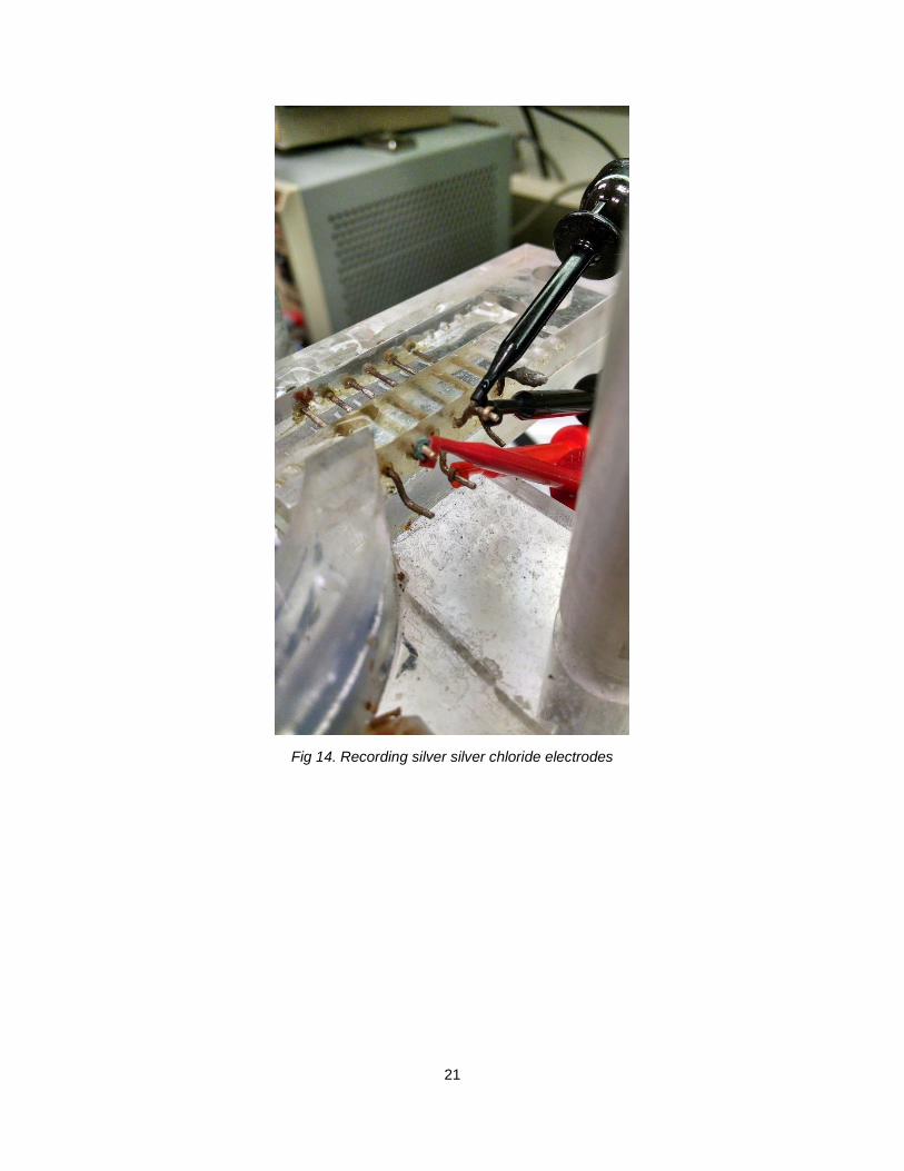
of the bath where the nerve loop is exposed to the Ultrasound. They are thick silver-silver
chloride electrodes on which the other end of the nerve is draped as shown in Fig 14. It is at a
higher level than the usual level of Ringer’s solution to avoid any unwanted artefacts.
21
Fig 14. Recording silver silver chloride electrodes
22
CHAPTER 4
RESULTS
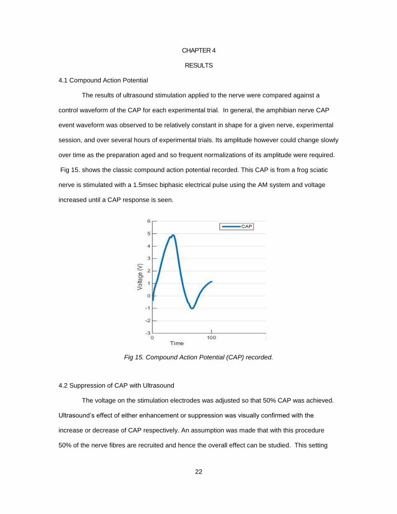
4.1 Compound Action Potential
The results of ultrasound stimulation applied to the nerve were compared against a
control waveform of the CAP for each experimental trial. In general, the amphibian nerve CAP
event waveform was observed to be relatively constant in shape for a given nerve, experimental
session, and over several hours of experimental trials. Its amplitude however could change slowly
over time as the preparation aged and so frequent normalizations of its amplitude were required.
Fig 15. shows the classic compound action potential recorded. This CAP is from a frog sciatic
nerve is stimulated with a 1.5msec biphasic electrical pulse using the AM system and voltage
increased until a CAP response is seen.
Fig 15. Compound Action Potential (CAP) recorded.
4.2 Suppression of CAP with Ultrasound
The voltage on the stimulation electrodes was adjusted so that 50% CAP was achieved.
Ultrasound’s effect of either enhancement or suppression was visually confirmed with the
increase or decrease of CAP respectively. An assumption was made that with this procedure
50% of the nerve fibres are recruited and hence the overall effect can be studied. This setting
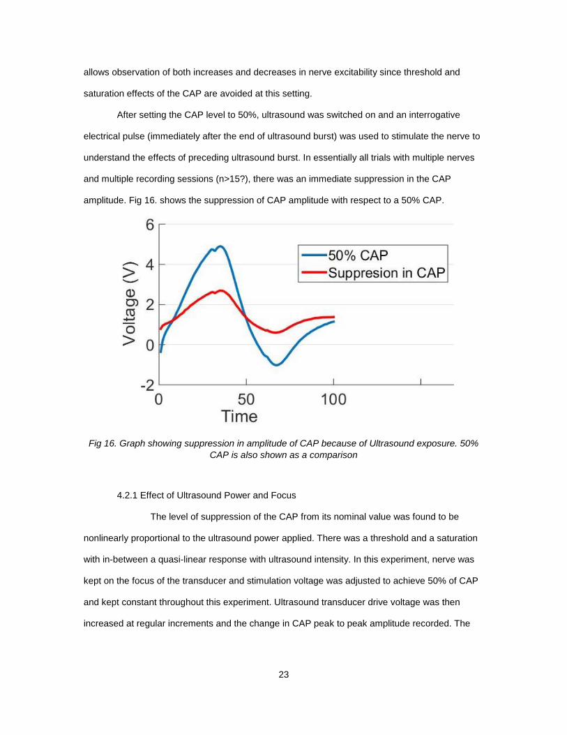
23
allows observation of both increases and decreases in nerve excitability since threshold and
saturation effects of the CAP are avoided at this setting.
After setting the CAP level to 50%, ultrasound was switched on and an interrogative
electrical pulse (immediately after the end of ultrasound burst) was used to stimulate the nerve to
understand the effects of preceding ultrasound burst. In essentially all trials with multiple nerves
and multiple recording sessions (n>15?), there was an immediate suppression in the CAP
amplitude. Fig 16. shows the suppression of CAP amplitude with respect to a 50% CAP.
Fig 16. Graph showing suppression in amplitude of CAP because of Ultrasound exposure. 50%
CAP is also shown as a comparison
4.2.1 Effect of Ultrasound Power and Focus
The level of suppression of the CAP from its nominal value was found to be
nonlinearly proportional to the ultrasound power applied. There was a threshold and a saturation
with in-between a quasi-linear response with ultrasound intensity. In this experiment, nerve was
kept on the focus of the transducer and stimulation voltage was adjusted to achieve 50% of CAP
and kept constant throughout this experiment. Ultrasound transducer drive voltage was then
increased at regular increments and the change in CAP peak to peak amplitude recorded. The
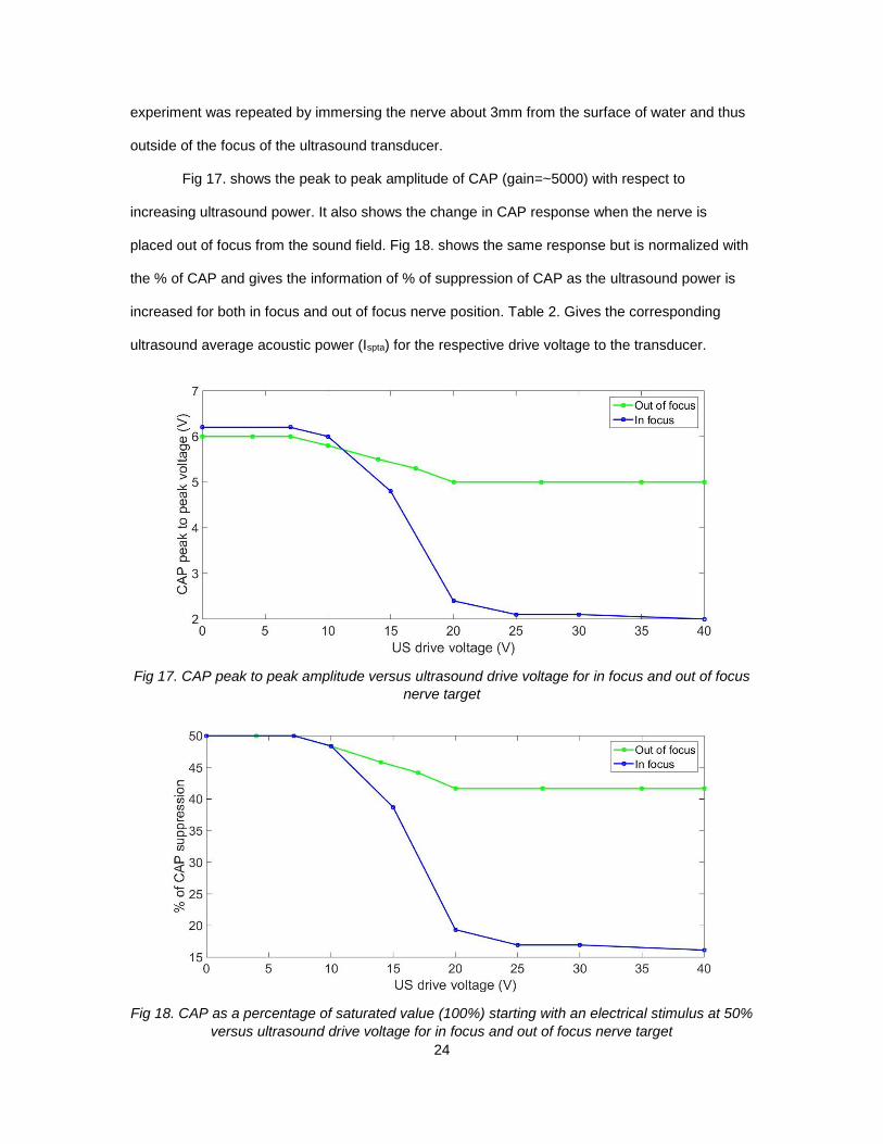
24
experiment was repeated by immersing the nerve about 3mm from the surface of water and thus
outside of the focus of the ultrasound transducer.
Fig 17. shows the peak to peak amplitude of CAP (gain=~5000) with respect to
increasing ultrasound power. It also shows the change in CAP response when the nerve is
placed out of focus from the sound field. Fig 18. shows the same response but is normalized with
the % of CAP and gives the information of % of suppression of CAP as the ultrasound power is
increased for both in focus and out of focus nerve position. Table 2. Gives the corresponding
ultrasound average acoustic power (Ispta) for the respective drive voltage to the transducer.
Fig 17. CAP peak to peak amplitude versus ultrasound drive voltage for in focus and out of focus
nerve target
Fig 18. CAP as a percentage of saturated value (100%) starting with an electrical stimulus at 50%
versus ultrasound drive voltage for in focus and out of focus nerve target
25
Ultrasound
transducer drive
voltage (V)
Corresponding
Average power (Ispta)
(mW/cm2)
10 ~28
15 53.58
20 131.171
25 182.90
30 232.80
35 264.20
40 323
Table 2. Ultrasound transducer voltage’s corresponding average acoustic power.
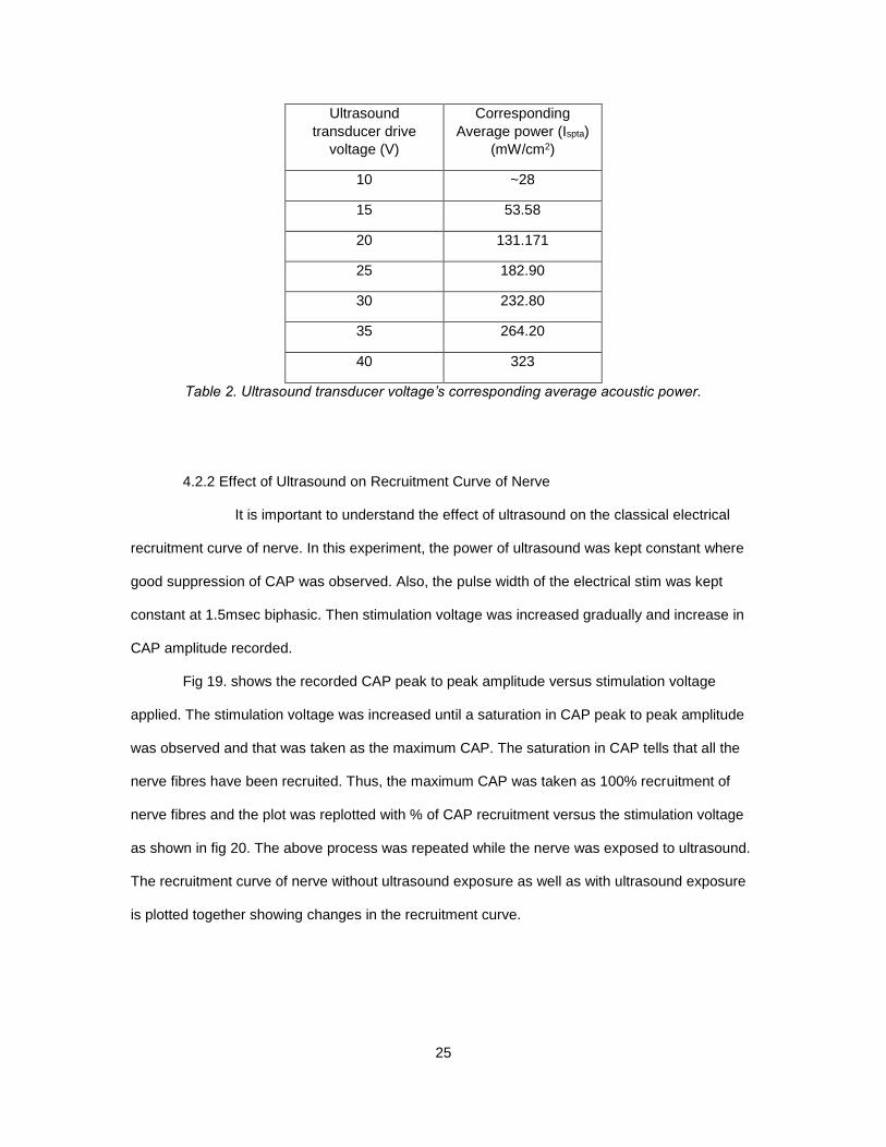
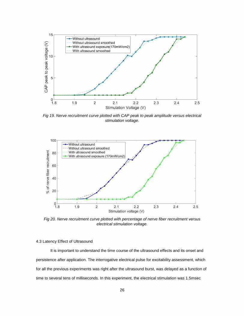
4.2.2 Effect of Ultrasound on Recruitment Curve of Nerve
It is important to understand the effect of ultrasound on the classical electrical
recruitment curve of nerve. In this experiment, the power of ultrasound was kept constant where
good suppression of CAP was observed. Also, the pulse width of the electrical stim was kept
constant at 1.5msec biphasic. Then stimulation voltage was increased gradually and increase in
CAP amplitude recorded.
Fig 19. shows the recorded CAP peak to peak amplitude versus stimulation voltage
applied. The stimulation voltage was increased until a saturation in CAP peak to peak amplitude
was observed and that was taken as the maximum CAP. The saturation in CAP tells that all the
nerve fibres have been recruited. Thus, the maximum CAP was taken as 100% recruitment of
nerve fibres and the plot was replotted with % of CAP recruitment versus the stimulation voltage
as shown in fig 20. The above process was repeated while the nerve was exposed to ultrasound.
The recruitment curve of nerve without ultrasound exposure as well as with ultrasound exposure
is plotted together showing changes in the recruitment curve.
26
Fig 19. Nerve recruitment curve plotted with CAP peak to peak amplitude versus electrical
stimulation voltage.
Fig 20. Nerve recruitment curve plotted with percentage of nerve fiber recruitment versus
electrical stimulation voltage.
4.3 Latency Effect of Ultrasound
It is important to understand the time course of the ultrasound effects and its onset and
persistence after application. The interrogative electrical pulse for excitability assessment, which
for all the previous experiments was right after the ultrasound burst, was delayed as a function of
time to several tens of milliseconds. In this experiment, the electrical stimulation was 1.5msec
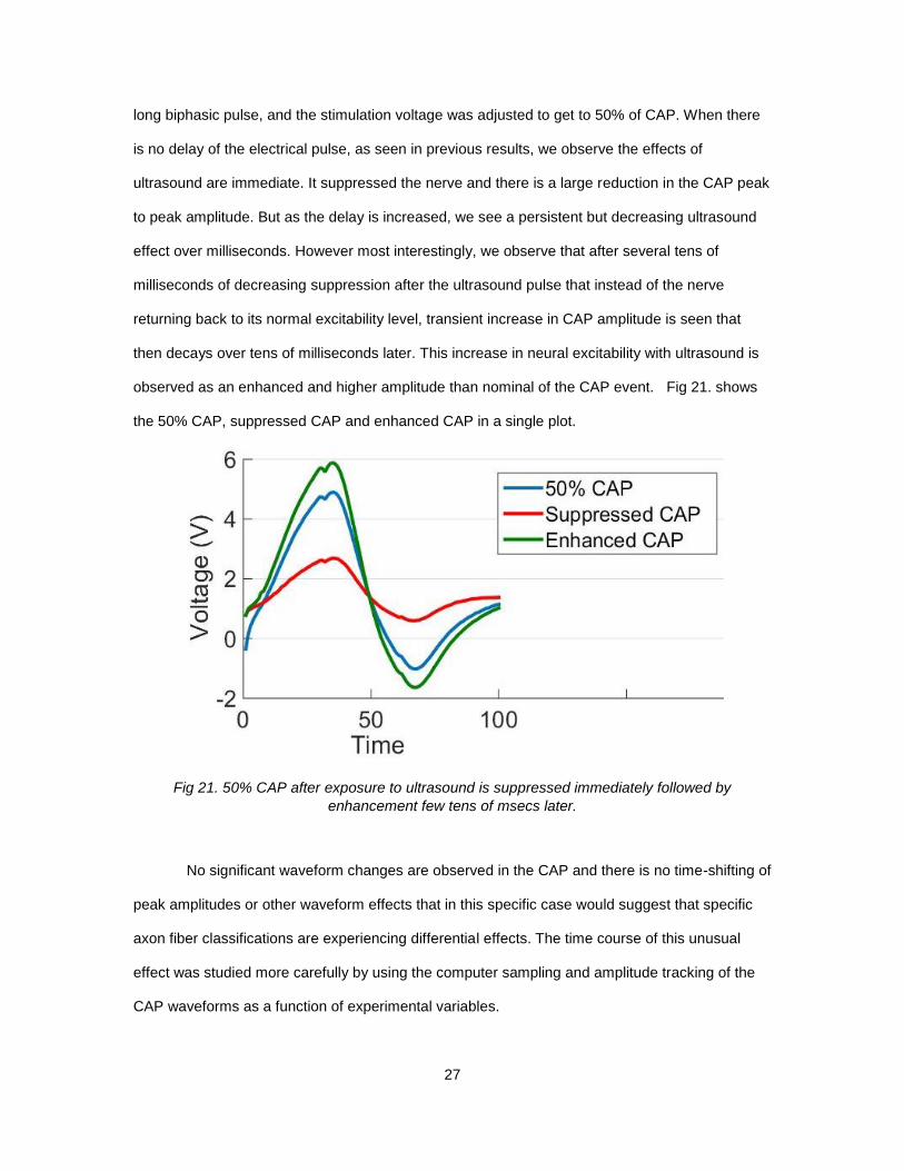
27
long biphasic pulse, and the stimulation voltage was adjusted to get to 50% of CAP. When there
is no delay of the electrical pulse, as seen in previous results, we observe the effects of
ultrasound are immediate. It suppressed the nerve and there is a large reduction in the CAP peak
to peak amplitude. But as the delay is increased, we see a persistent but decreasing ultrasound
effect over milliseconds. However most interestingly, we observe that after several tens of
milliseconds of decreasing suppression after the ultrasound pulse that instead of the nerve
returning back to its normal excitability level, transient increase in CAP amplitude is seen that
then decays over tens of milliseconds later. This increase in neural excitability with ultrasound is
observed as an enhanced and higher amplitude than nominal of the CAP event. Fig 21. shows
the 50% CAP, suppressed CAP and enhanced CAP in a single plot.
Fig 21. 50% CAP after exposure to ultrasound is suppressed immediately followed by
enhancement few tens of msecs later.
No significant waveform changes are observed in the CAP and there is no time-shifting of
peak amplitudes or other waveform effects that in this specific case would suggest that specific
axon fiber classifications are experiencing differential effects. The time course of this unusual
effect was studied more carefully by using the computer sampling and amplitude tracking of the
CAP waveforms as a function of experimental variables.
28
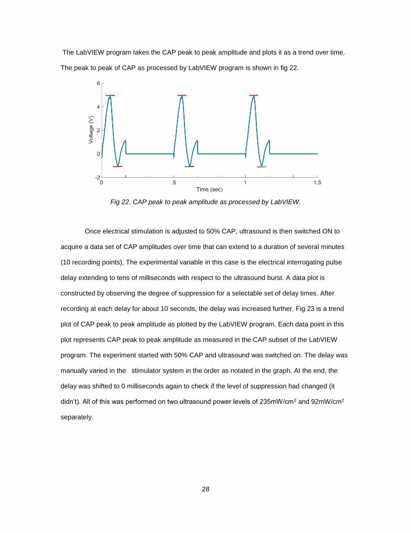
The LabVIEW program takes the CAP peak to peak amplitude and plots it as a trend over time.
The peak to peak of CAP as processed by LabVIEW program is shown in fig 22.
Fig 22. CAP peak to peak amplitude as processed by LabVIEW.
Once electrical stimulation is adjusted to 50% CAP, ultrasound is then switched ON to
acquire a data set of CAP amplitudes over time that can extend to a duration of several minutes
(10 recording points), The experimental variable in this case is the electrical interrogating pulse
delay extending to tens of milliseconds with respect to the ultrasound burst. A data plot is
constructed by observing the degree of suppression for a selectable set of delay times. After
recording at each delay for about 10 seconds, the delay was increased further. Fig 23 is a trend
plot of CAP peak to peak amplitude as plotted by the LabVIEW program. Each data point in this
plot represents CAP peak to peak amplitude as measured in the CAP subset of the LabVIEW
program. The experiment started with 50% CAP and ultrasound was switched on. The delay was
manually varied in the stimulator system in the order as notated in the graph. At the end, the
delay was shifted to 0 milliseconds again to check if the level of suppression had changed (it
didn’t). All of this was performed on two ultrasound power levels of 235mW/cm2 and 92mW/cm2
separately.
29
Fig 23. Trend plot of CAP peak to peak amplitude showing the change from inhibition to
enhancement of the nerve.
The data set as seen in fig 23 is recorded from the nerve of a single frog and is a
representation of several experiments conducted. Similar experiments were performed on 12
sciatic nerves of 8 frogs of the same species over a period of 18 months. We always observed
similar response where ultrasound caused huge inhibition and increased excitation about 16-22
milliseconds after the ultrasound burst. Some of those data sets are shown in appendix A.
Since the above experiment was conducted in a way where the delay of electrical
stimulation was manually changed in the order, it could be concluded that the step changes
observed could be as a result of step increase in the delay. Though the same kind of response
was observed in several experiments, we also performed experiments where the delay was set at
one delay time and the changes were observed. The experiment was repeated for a different
delay and we observed that the response was very similar to as seen in fig 23. For example, at 0
msecs delay, we always observed big time inhibition while at 22 or 24 msecs, we always
observed excitation. Thus, we can strongly conclude that the response observed above is only
because of ultrasound and not the sequence or progressive step changes in delay.
The data points of within a given delay from the above graph were subsequently
manually averaged to plot the relative CAP peak to peak amplitude versus the delay of the
electrical stimulation as shown in fig. 24. This reduced plot of fig. 24 more clearly shows the time
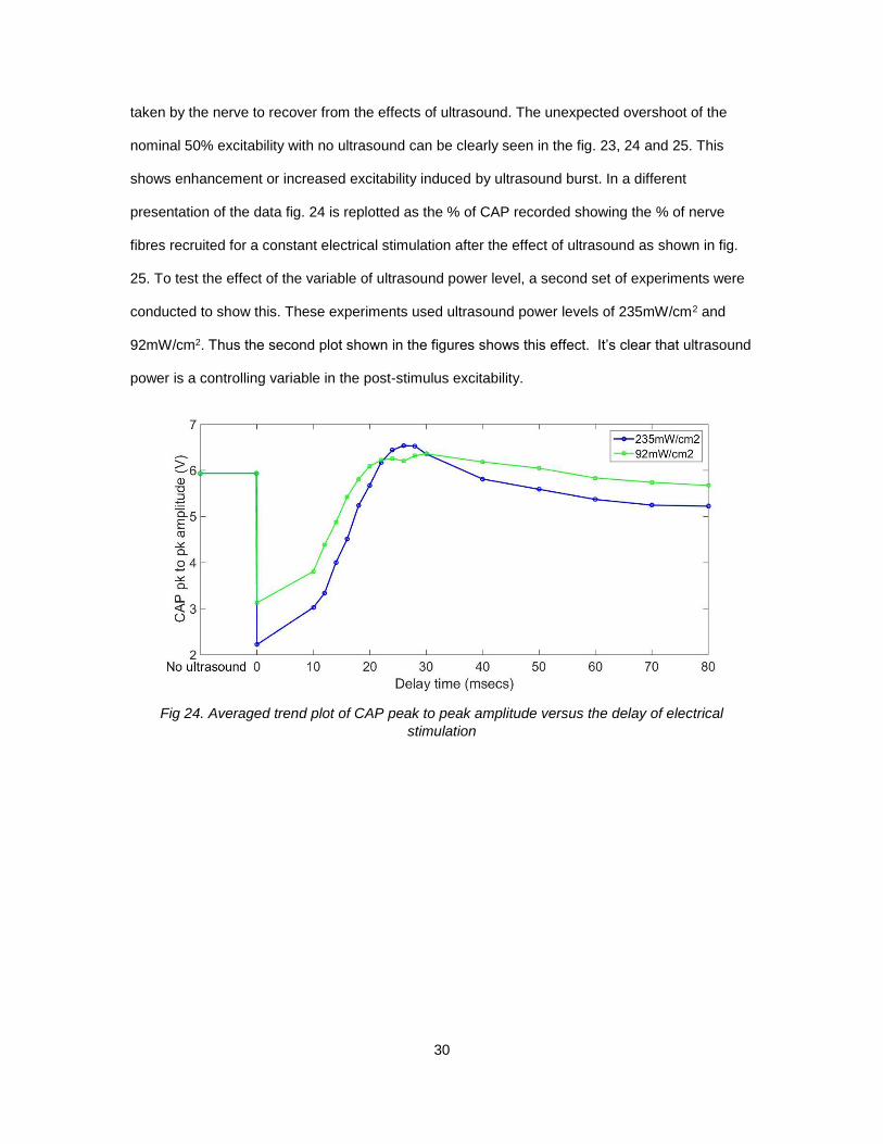
30
taken by the nerve to recover from the effects of ultrasound. The unexpected overshoot of the
nominal 50% excitability with no ultrasound can be clearly seen in the fig. 23, 24 and 25. This
shows enhancement or increased excitability induced by ultrasound burst. In a different
presentation of the data fig. 24 is replotted as the % of CAP recorded showing the % of nerve
fibres recruited for a constant electrical stimulation after the effect of ultrasound as shown in fig.
25. To test the effect of the variable of ultrasound power level, a second set of experiments were
conducted to show this. These experiments used ultrasound power levels of 235mW/cm2 and
92mW/cm2. Thus the second plot shown in the figures shows this effect. It’s clear that ultrasound
power is a controlling variable in the post-stimulus excitability.
Fig 24. Averaged trend plot of CAP peak to peak amplitude versus the delay of electrical
stimulation
31
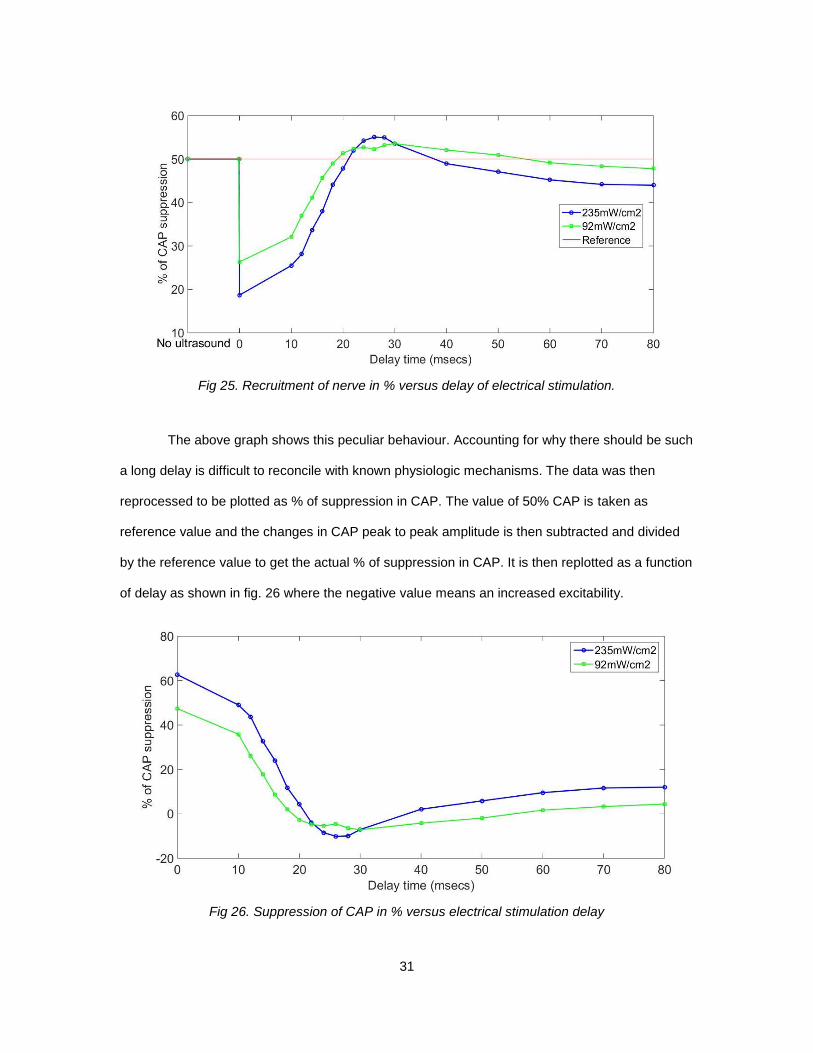
Fig 25. Recruitment of nerve in % versus delay of electrical stimulation.
The above graph shows this peculiar behaviour. Accounting for why there should be such
a long delay is difficult to reconcile with known physiologic mechanisms. The data was then
reprocessed to be plotted as % of suppression in CAP. The value of 50% CAP is taken as
reference value and the changes in CAP peak to peak amplitude is then subtracted and divided
by the reference value to get the actual % of suppression in CAP. It is then replotted as a function
of delay as shown in fig. 26 where the negative value means an increased excitability.
Fig 26. Suppression of CAP in % versus electrical stimulation delay
32
4.4 Effect of Ultrasound on Strength-Duration curve
To better understand how ultrasound effects the peripheral nerve, an experiment was
conducted to plot its effect on the chronaxie of sciatic nerve. Chronaxie gives insight into nerve
membrane electrical characteristics and would be expected to be a sensitive indicator of any
ultrasound-induced effects on these properties of nerve. In this experiment, the ultrasound is
held constant and the pulse width of the electrical stimulation is increased gradually from 20µsec
until 2 msecs while the voltage is adjusted to get about 50% of CAP. Prior to this, maximum
possible CAP amplitude (100% recruitment) is recorded at 1msec biphasic pulse and 50% of
CAP is calculated from that. Then the voltage of electrical stimulation required to achieve 50% of
CAP peak to peak amplitude is recorded for pulse width from 20µsec to 2msec. This process is
then repeated for an ultrasound affected nerve at a power level of 56mW/cm2. Before the
recording of the ultrasound affected nerve is started, the initial steps of verifying the maximum
possible CAP amplitude (100% recruitment) is repeated at 1msec biphasic pulse to ensure that
value of max peak to peak CAP voltage has not changed due to either nerve drying out or other
environmental factors.
The pulse width of electrical stimulation is then plotted versus voltage required to get
50% CAP for both ultrasound affected nerve and just the electrical stimulation on the nerve as
shown in fig 27. This plot shows data that was able to be recorded with good precision. It is
representative (but not average) of multiple trials (N=2) made on different nerves and different
experimental sessions. It can be seen from the figure that ultrasound application has small effect
on membrane chronaxie to the right side of the plot but some effect in the range where very short
electrical pulse durations at high amplitudes are recorded.
A close up view of the initial part of the chronaxie curve is as shown in fig 28. There is a
huge increase in the voltage required to stimulate the nerve at the shorter pulse width’s than it is
at the longer pulse width’s. The rheobase was found to be 0.225V for without ultrasound and
0.36V with the effect of ultrasound. Based on the formula, the chronaxie line was drawn at 0.45V
for just the electrical stimulation and 0.72 for with the ultrasound exposure data. The chronaxie
33
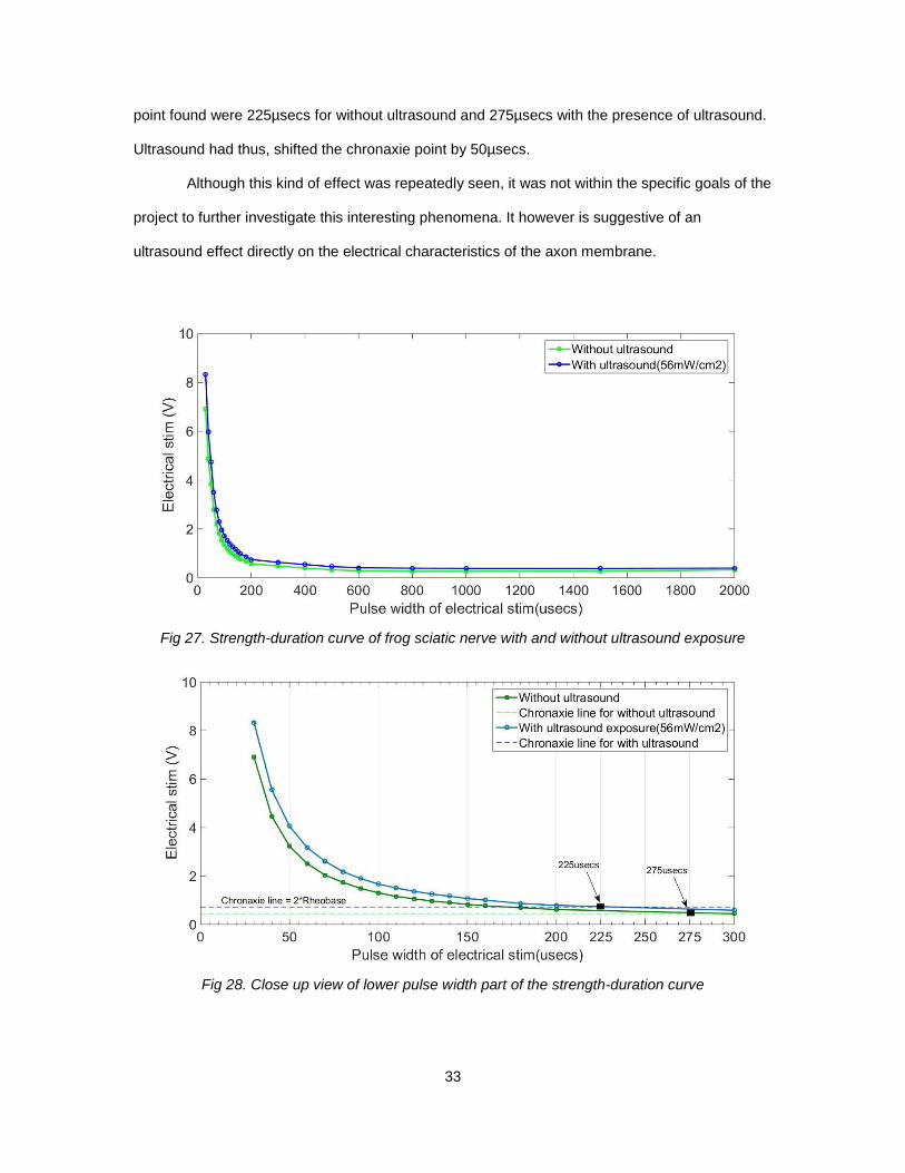
point found were 225µsecs for without ultrasound and 275µsecs with the presence of ultrasound.
Ultrasound had thus, shifted the chronaxie point by 50µsecs.
Although this kind of effect was repeatedly seen, it was not within the specific goals of the
project to further investigate this interesting phenomena. It however is suggestive of an
ultrasound effect directly on the electrical characteristics of the axon membrane.
Fig 27. Strength-duration curve of frog sciatic nerve with and without ultrasound exposure
Fig 28. Close up view of lower pulse width part of the strength-duration curve
34
The strength-duration curve as shown in literature is usually done for a stimulation
voltage that can just drive the nerve into firing. In our case, we had used 50% of CAP value and
the rationale behind this was to be able to compare our previous results where every experiment
conducted to understand the effects of ultrasound were done at 50% of CAP peak to peak value.
Another difficulty faced in not only this but every prior experiments were the time factor
for conducting the experiments. Due to environmental conditions, it was difficult to maintain
moisture on the nerve and as the nerve dried out, its excitability reduced. We then used to spray
ringer’s solution and also dip the nerve completely in ringer’s bath that caused slight shift in the
excitability of nerve. Thus, most of the data shown in all sections of this chapter is a
representation of several experiments conducted on 18 sciatic nerves from 12 bullfrogs over a
period of 18 months. As it was difficult to get the same excitability in different nerves, across
different time of the experiment, we stuck to performing major part of the experiments at 50%
CAP peak to peak value.
4.5 Morphology changes in CAP
It was found that apart from suppression in amplitude of CAP, ultrasound also affects the
CAP waveform. The LabVIEW program has the capability of plotting an ensemble (n>50 events)
of all the CAP’s recorded for an experiment. It was observed that in many, but not all
experiments, there were changes in waveform shape as shown in fig. 29. It is well known that
CAP waveform morphology is a strong function of the position of recording electrodes such as
their separation and recording differential versus monopolar. However relative changes in CAP
shape as a function of other system variables such as ultrasound application can be taken as
indicative of some basic physiologic event. This study did not extensively pursue the
observations of CAP waveform changes as an experimental variable. However, it was noticed
that significant waveform changes are clearly possible with ultrasound application. This suggests
that ultrasound might not only have effects on membrane excitability but also differentially;
perhaps on axon fiber types or membrane ion channel kinetics.
35
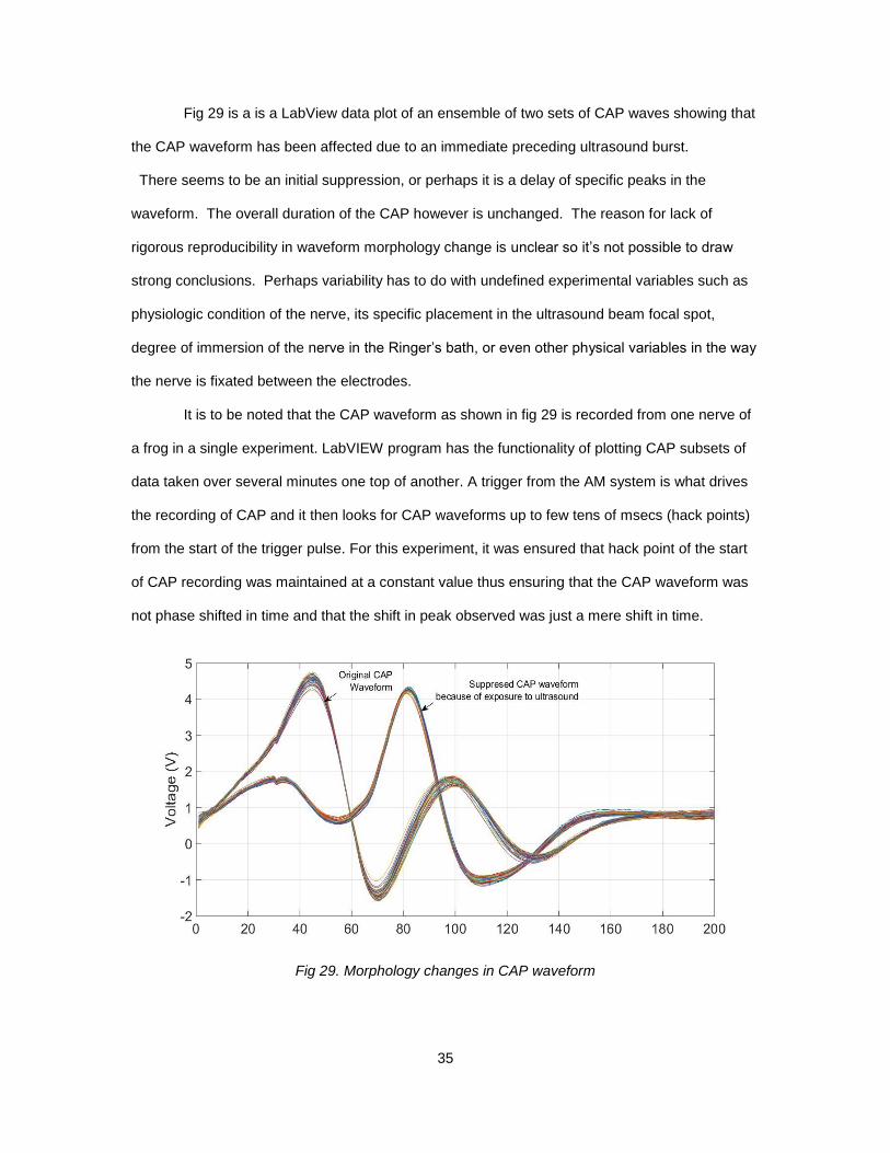
Fig 29 is a is a LabView data plot of an ensemble of two sets of CAP waves showing that
the CAP waveform has been affected due to an immediate preceding ultrasound burst.
There seems to be an initial suppression, or perhaps it is a delay of specific peaks in the
waveform. The overall duration of the CAP however is unchanged. The reason for lack of
rigorous reproducibility in waveform morphology change is unclear so it’s not possible to draw
strong conclusions. Perhaps variability has to do with undefined experimental variables such as
physiologic condition of the nerve, its specific placement in the ultrasound beam focal spot,
degree of immersion of the nerve in the Ringer’s bath, or even other physical variables in the way
the nerve is fixated between the electrodes.
It is to be noted that the CAP waveform as shown in fig 29 is recorded from one nerve of
a frog in a single experiment. LabVIEW program has the functionality of plotting CAP subsets of
data taken over several minutes one top of another. A trigger from the AM system is what drives
the recording of CAP and it then looks for CAP waveforms up to few tens of msecs (hack points)
from the start of the trigger pulse. For this experiment, it was ensured that hack point of the start
of CAP recording was maintained at a constant value thus ensuring that the CAP waveform was
not phase shifted in time and that the shift in peak observed was just a mere shift in time.
Fig 29. Morphology changes in CAP waveform
36
CHAPTER 5
DISCUSSION
5.1 Suppression of Compound Action Potential (CAP)
Ultrasound, as shown by several other authors in the past[2]–[4], [8], [7], [5], has a
suppressive effect on the electrical excitability of peripheral nerve. As shown in the section 4.2, a
burst of ultrasound can cause a given electrical stimulus to have a considerably lesser effect.
The level of suppression was tested in this work at a fixed ultrasound frequency and as a function
of ultrasound power. It shows that
1. The higher the power of the ultrasound, the greater is the inhibition of the nerve. The
ultrasound recruitment curve clearly demonstrates this since as the drive on the
ultrasound transducer was increased (indicative of increase in ultrasound power), the %
of suppression in the nerve increased.
2. Focusing of the ultrasound beam cooroborates this effect since the nerve was in the
exact focal spot of the ultrasound transducer, the level of suppression was high as when
compared to when the nerve was submerged in the Ringer’s solution and out of focal
spot.
The effect of ultrasound frequency and ultrasound pulse train characteristics applied to
the nerve were not a variable in this study. The 5 MHz ultrasound transducer frequency in
combination with its focusing created millimetre-order focal spots. The focal region was thus able
to capture the entire diameter of the amphibian nerve and support the assumption that the nerve
was in a quasi-uniform ultrasound field.
5.1.1 Mechanosensitive hypothesis
A hypothesis concerning this inhibition could be that its attributable to the
mechanosensitive property of the voltage-gated ion channels (Na+, Ca++ & K+). It has been
previously shown that these ion channels are stretch-sensitive and respond to tension applied on
the lipid bilayer. When the nerve is in the focal zone of the ultrasound, a periodic pressure is
applied on the cell membrane and it is expected to result in a periodic tension-relaxation on the
lipid bilayer. It could be that the this effect around the lipid bilayer of the nerve fibres causes a
37
temporary scrambling of function of the voltage gated ion channels as it undergoes the acoustic
radiation forces [20]. This can result in the nerve being less excitable to external stimuli which is
what is seen as suppression.
5.2 Recruitment curve
A classic S-shaped response curve was observed when electrical stimulation was
increased stepwise until no further increase in CAP amplitude was observed. This was an
indication that the nerve was very much working and alive during our experiments.
When the level of suppression was held constant as an experimental variable and the
nerve exposed to ultrasound, there was a corresponding and significant increase in the voltage
required to recruit it back to the 50% point. This is consistent with experiments that showed that
there was a significant inhibition observed when the nerve was exposed to ultrasound. Thus the
effect of ultrasound inhibition can be overcome by applying an increased electrical stimulus and
does not appear to interfere with the further action of electrical stimulation.
5.2.1 Recruitment fibre theory
Another interesting thing of note in this recruitment curve (fig 6) is the difference in
voltage required to stimulate 20% as compared to 90%. On carefully analysing the graph, we see
that it takes about 200mV more to achieve 20% of nerve fibre recruitment as compared to
approximately 100mV more at 90% recruitment when the nerve is exposed to ultrasound. This
effect may be indicative of a differential ultrasound effect on different fibre types. Considering the
theory behind the recruitment curve where the faster fibres are among the 1st ones to be recruited
(when a low voltage electrical stim is applied) followed by the slower ones, this suggests that the
ultrasound has a larger inhibitive effect on the faster fibres as when compared to the slower ones.
5.3 The overshoot followed after inhibition
While it is very interesting to observe the ultrasound’s ability to inhibit the nerve, it is
equally very important to understand the time course of ultrasound inhibition since it is unlike that
of electrical stimulation. For practical applications in neuromodulation, it is important that
38
ultrasound effects are relatively short lived to achieve high pulse repetition rates. Are ultrasound
effects something that is completely irreversible or can the nerve return to its normal state? How
long does it take to return to its normal state?
The experiment that plotted the nerve excitability as a function of delay after ultrasound
burst gives insight into this. The trend plot in fig 9 shows that the ultrasound effect decays after
pulse and the nerve returns to its nominal excitability (before it was inhibited by ultrasound) in
about 18-20msecs. However, interrupting this smooth decay is an apparent overshoot to an
increase excitability before ultimate return to nominal. The nerve is behaving somewhat like an
underdamped system. Instead of just staying at its nominal value, we observed an overshoot in
the CAP peak to peak amplitude, a clear indication of an underdamped type of response causing
an excitability enhancement in the nerve. Table 3 gives the maximum observed inhibition and
overshoot for the two ultrasound power level.
Ultrasound power level
(mW/cm2)
Maximum inhibition
observed (%)
Maximum overshoot
observed (%)
225 47 5
540 62 10
Table 3. Maximum level of inhibition and overshoot for 2 ultrasound power level
It is to be noted that the level of excitation is comparatively small relative to the
suppression. We observe from this limited data set that excitatory effects increase as the
ultrasound power level is increased.
5.3.1 Wear out effect and Mechanosensitivity of the nerve
One of the hypothesis behind this overshoot can be the general recovery process
of the nerve causing the overshoot. As the nerve recovers from the effect of ultrasound, the
voltage-gated ion channels begin to open slowly and recover from forced closure. Now when we
apply an electrical stimulus let’s say at 22msecs after the ultrasound burst, it could be that the
39
external force causes an increase in the channel opening resulting in more influx and outflux of
ions in the fibres. This increased ion changes can result in the enhancement seen.
Also, it has been shown that the voltage-gated ion channels are sensitive to mechanical
pressure on the lipid bilayer[20][21]. The acoustic pressure exerted on the nerve due to
ultrasound can cause tension in the lipid bilayer. The primary effect of this tension could be
inhibitive but as the ultrasound is off, this acoustic pressure slowly reduces on the nerve and
during this process, could have made the ion channels more sensitive causing an increase in
CAP amplitude.
5.3.2 Activation of ion channels
As a follow up of the previous hypothesis, there has been research done which
shows that ultrasound is capable of stimulating and modulating sodium and calcium channel
conductance’s [22]. The authors showed an increase in the Na+ and Ca2+ activity when low
intensity low frequency ultrasound was introduced. The same activity could have resulted in the
overshoot seen.
5.3.3 Stretch inhibition and activation
Another hypothesis behind the observed inhibition and activation could be
because of the stretching of the nerve. When ultrasound is directed at the nerve (which is very
close to the ringer solution and air interface), a complex sound field exists at the surface of water
which causes a shearing effect on the nerve. The nerve is pulled and squished because of the
acoustic radiation force which can cause stretching. It has been shown in reported literature
studies [4], [8], [23], that nerve can be both excited and inhibited if stretched and the same
response is seen here as it first undergoes inhibition and followed by excitation.
5.3.4 Fibre specificity
Another hypothesis for the overshoot could be that ultrasound effects different
fibres differently. With the recruitment curve showing that the difference in voltage required to
recruit the nerve with and without ultrasound is higher at 20% than 90%, it can be that as the
ultrasound inhibits the faster myelinated fibres, it could enhance the slow moving fibres. The
rationale behind this can be the significant difference in the level of overshoot when compared to
40
the inhibition. At 50% recruitment, we can expect to see more of the faster myelinated fibres
being recruited than the slower unmyelinated fibres. Since the number of these slow fibres are
less, less of an overshoot is observed.
5.4 Chronaxie shift
Chronaxie is a characteristic pulse duration which is usually considered as an ideal time
that can stimulate the nerve at the least possible energy. In the strength-duration curve of the
nerve with and without ultrasound, we observe a visible upward shift in the ultrasound exposed
nerve curve compared to the control. There was also a shift of about 50µsecs in the chronaxie
value suggesting that ultrasound has effected the conduction of the suppressed nerve. On taking
a closer look, we also observe that the voltage required to recruit 50% of suppressed nerve was
higher at shorter durations of pulse width than the longer ones. Thus this suggests of an
ultrasound effect on membrane characteristics such as equivalent values of resistance and
capacitance. Presumably a nerve patch-clamp study would reveal more of the details.
5.5 Morphology change
On plotting an ensemble of CAP waveforms of both normal and suppressed nerve, we
often saw a change in the waveform shape. Initially it was thought that there was a shift of CAP
waveform in the time axis however this is not the case. Both the control and ultrasound applied
waveforms end at the same time. We thus conclude that there is an actual change in the CAP
waveform.
Additionally, from the graph, it is noted that there is a change in the peak of the CAP
waveform. The original CAP waveforms has a very clear two peaked nature, presumably showing
the response of the faster as well as the slower fibres. But when ultrasound is applied, we see a
reduction in the first peak followed by an increased new peak few 100’s of µsecs later. This
behaviour is difficult to account without techniques to more fully determine how different
populations of nerve fibre type within the axon are individually behaving.
41
CHAPTER 6
CONCLUSION
In this work, the neuromodulatory effects of ultrasound was studied using a peripheral
nerve model of amphibian. One of the major findings from the several experiments conducted is
the ability of ultrasound to cause both suppression and increased excitability of the amphibian
axon at the point of electrical stimulation. This effect on excitability of neruronal activity is an
important thing in neuromodulation. Several previous literature works suggested that the primary
neuromodulatory effect of high frequency ultrasound results from an instantaneous rise in
temperature. Our findings strongly suggest the possible existence of a more mechanical
(radiation force) and fiber-sensitive effect of ultrasound. Further in-depth studies need to
conducted to better understand the exact mechanism behind the neuromodulatory effect of
ultrasound on peripheral nerves. It could be that a combination of all the parameters like transient
temperature rise, mechanical radiation force and fiber specificity contribute to the high inhibition
and comparatively low excitation as observed in our results.
This study suggests future work can be as follows:
1. Blocking different types of fibres to verify the fibre-specific effect of ultrasound as
observed in the strength-duration curve and recruitment curve.
2. Evaluating the effect of ultrasound frequency on the level of inhibition and enhancement
by repeating the experiments on lower frequency (400kHz-2.5MHz) and higher frequency
(above 10MHz).
3. Performing in-vivo experiments to check for response of ultrasound when the peripheral
nerve is inside of a body.
This study explores the possible use of a focused high frequency ultrasound either in
tandem with an electrical stimulation or just by itself to effectively modulate the nerve. One of the
major advantages of using high frequency ultrasound is its ability to focus to very small
diameters, which are deep inside the tissues and deposit highly focused and localized energy,
something which is not possible by optical or electrical stimulation methods non-invasively. With
the current advances in technology, high frequency ultrasound can be used to sweep peripheral

42
nerves deep into the tissues and modulate the excitability of the nerve which can be used to
improve the spatial specificity of electrical stimulation.
43
REFERENCE
[1] “International Neuromodulation Society. Welcome to the International Neuromodulation
Society.” [Online]. Available: www.neuromodulation.com. [Accessed: 22-Jan-2013].
[2] V. Colucci, G. Strichartz, F. Jolesz, N. Vykhodtseva, and K. Hynynen, “Focused
Ultrasound Effects on Nerve Action Potential in vitro,” Ultrasound Med. Biol., vol. 35, no.
10, pp. 1737–1747, 2009.
[3] E. J. Juan, R. González, G. Albors, M. P. Ward, and P. Irazoqui, “Vagus nerve modulation
using focused pulsed ultrasound: Potential applications and preliminary observations in a
rat,” Int. J. Imaging Syst. Technol., vol. 24, no. 1, pp. 67–71, 2014.
[4] R. T. Mihran, F. S. Barnes, and H. Wachtel, “Temporally-specific modification of
myelinated axon excitability in vitro following a single ultrasound pulse,” Ultrasound Med.
Biol., vol. 16, no. 3, pp. 297–309, 1990.
[5] W. B. Phillips, “High Frequency Ultrasound Modifications to the Electrical Activation of
Neural Tissue,” Arizona State University, 2008.
[6] P. H. Tsui, S. H. Wang, and C. C. Huang, “In vitro effects of ultrasound with different
energies on the conduction properties of neural tissue,” Ultrasonics, vol. 43, no. 7, pp.
560–565, 2005.
[7] S. F. Takagi, S. Higashino, T. Shibuya, and N. Osawa, “The Actions of Ultrasound on the
Myelinated Nerve, the Spinal Cord and the Brain,” Jpn. J. Physiol., vol. 10, no. 2, pp. 183–
193, 1960.
[8] R. T. Mihran, “Temporally-specific modulation of neuronal excitability by pulsed
ultrasound,” University of Colorado, 1990.
[9] 1816-1887 Ecker, Alexander and G. Haslam, The Anatomy of the Frog. Oxford: Clarendon
Press, 1889.
[10] “The McGill Physiology Virtual Lab.” [Online]. Available:
http://www.medicine.mcgill.ca/physio/vlab/cap/prep.htm. [Accessed: 15-Oct-2016].
[11] G. G. Matthews, Cellular Physiology of Nerve and Muscle (4). Wiley-Blackwell, 2009.
[12] Weiss and G., “Sur la possibilite de rendre comparables entre eux les appareils servant a
l’excitation electrique.,” Arch. Ital. Biol., vol. 35, no. 1, pp. 413–445, 1990.
[13] L. Lapicque, “Definition experimentale de l’excitabilite,” C. R. Acad. Sci., Paris, vol. 67, no.
280, p. 3, 1909.
[14] W. Irnich, “The Terms ‘Chronaxie’ and ‘Rheobase’ are 100 Years Old,” Pacing Clin.
Electrophysiol., vol. 33, no. 4, pp. 491–496, Apr. 2010.
[15] W. Irnich, “The Chronaxie Time and Its Practical Importance,” Pacing Clin. Electrophysiol.,
vol. 3, no. 3, pp. 292–301, May 1980.
[16] R. W. Wood and A. L. Loomis, “XXXVIII. The physical and biological effects of high-
44
frequency sound-waves of great intensity,” London, Edinburgh, Dublin Philos. Mag. J. Sci.,
vol. 4, no. 22, pp. 417–436, 1927.
[17] P. Dioszeghy and E. Stalberg, “Changes in motor and sensory nerve conduction
parameters with temperature in normal and diseased nerve,” Electroencephalogr Clin
Neurophysiol, vol. 85, no. 4, pp. 229–235, 1992.
[18] “Frog Ringer’s Solution,” 2003. [Online]. Available:
http://webs.wofford.edu/davisgr/bio342/Ringers.htm.
[19] K. Jaksukam and S. Umchid, “Development of ultrasonic power measurement standards
in Thailand,” in IEEE 2011 10th International Conference on Electronic Measurement &
Instruments, 2011, pp. 1–5.
[20] C. E. Morris and P. F. Juranka, “Lipid Stress at Play: Mechanosensitivity of Voltage-Gated
Channels,” 2007, pp. 297–338.
[21] S. Sukharev and D. P. Corey, “Mechanosensitive Channels: Multiplicity of Families and
Gating Paradigms,” Sci. Signal., vol. 2004, no. 219, p. re4-re4, Feb. 2004.
[22] W. J. Tyler, Y. Tufail, M. Finsterwald, M. L. Tauchmann, E. J. Olson, and C. Majestic,
“Remote Excitation of Neuronal Circuits Using Low-Intensity, Low-Frequency Ultrasound,”
PLoS One, vol. 3, no. 10, p. e3511, Oct. 2008.
[23] C. E. Morris and W. J. Sigurdson, “Stretch-inactivated ion channels coexist with stretch-
activated ion channels.,” Science, vol. 243, no. 4892, pp. 807–9, Feb. 1989.

45
APPENDIX A
ULTRASOUND LATENCY EFFECT DATA SETS
46
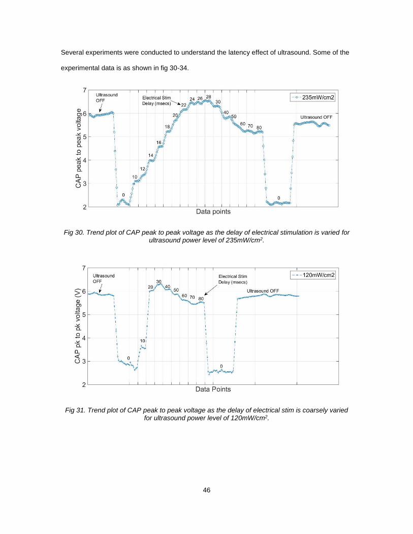
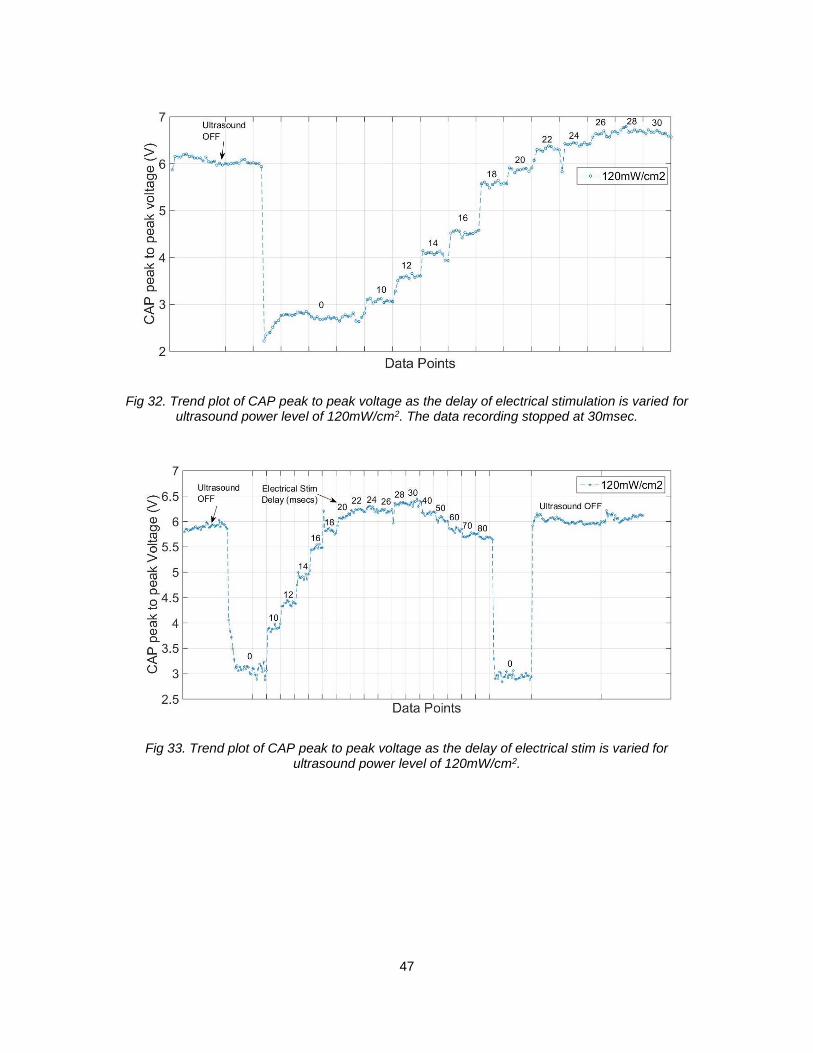
Several experiments were conducted to understand the latency effect of ultrasound. Some of the
experimental data is as shown in fig 30-34.
Fig 30. Trend plot of CAP peak to peak voltage as the delay of electrical stimulation is varied for ultrasound power level of 235mW/cm2.
Fig 31. Trend plot of CAP peak to peak voltage as the delay of electrical stim is coarsely varied for ultrasound power level of 120mW/cm2.
47
Fig 32. Trend plot of CAP peak to peak voltage as the delay of electrical stimulation is varied for ultrasound power level of 120mW/cm2. The data recording stopped at 30msec.
Fig 33. Trend plot of CAP peak to peak voltage as the delay of electrical stim is varied for ultrasound power level of 120mW/cm2.
48
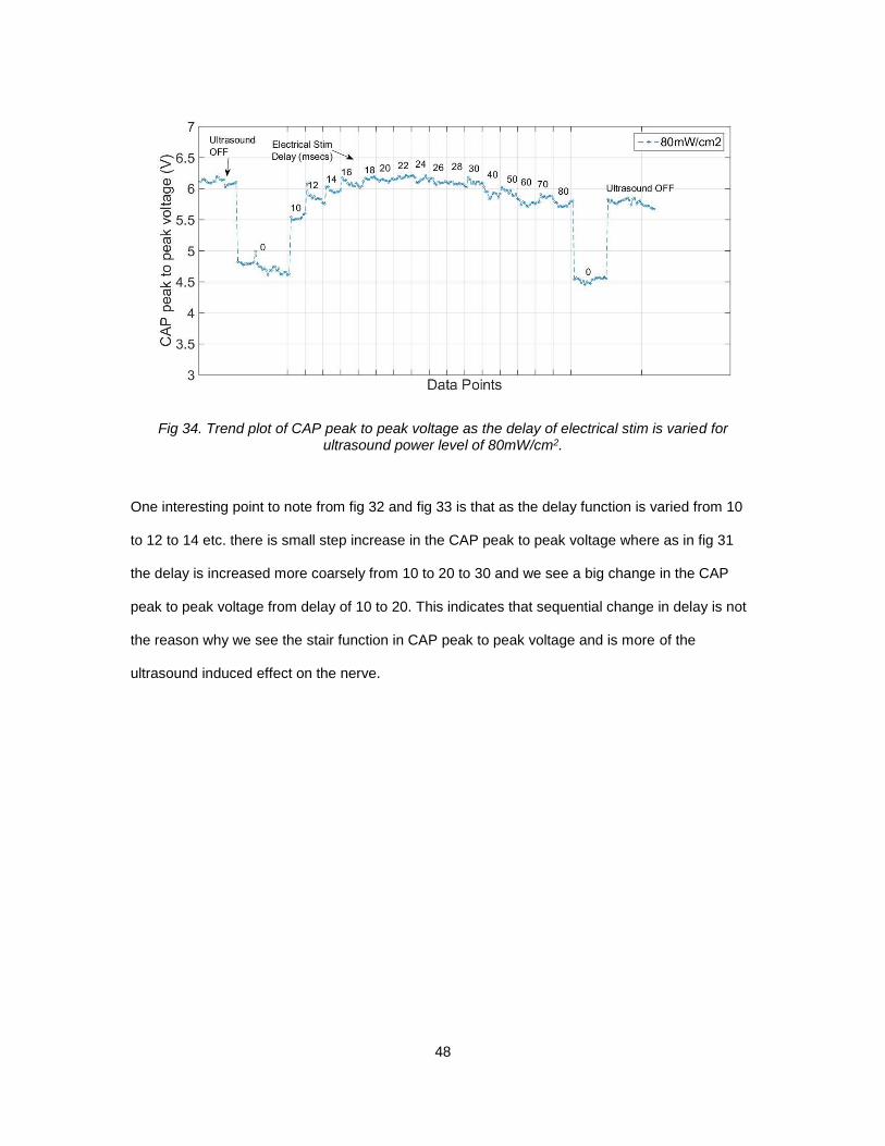
Fig 34. Trend plot of CAP peak to peak voltage as the delay of electrical stim is varied for ultrasound power level of 80mW/cm2.
One interesting point to note from fig 32 and fig 33 is that as the delay function is varied from 10
to 12 to 14 etc. there is small step increase in the CAP peak to peak voltage where as in fig 31
the delay is increased more coarsely from 10 to 20 to 30 and we see a big change in the CAP
peak to peak voltage from delay of 10 to 20. This indicates that sequential change in delay is not
the reason why we see the stair function in CAP peak to peak voltage and is more of the
ultrasound induced effect on the nerve.