Embed Size (px)
Citation preview

Neural Networks
Jiaming MaoXiamen University

Copyright © 2017–2019, by Jiaming Mao
This version: Spring 2019
Contact: [email protected]
Course homepage: jiamingmao.github.io/data-analysis
All materials are licensed under the Creative CommonsAttribution-NonCommercial 4.0 International License.

The Perceptron
Consider a binary classification problem.Let y ∈ {−1, 1} and x = (1, x1, . . . , xp).The perceptron is a linear classifier
h (x) = sign(w ′x
)that minimizes the misclassification loss
` (y , h (x)) = I (y 6= h (x))
w = (w0,w1, . . . ,wp) are weights.
© Jiaming Mao

The Perceptron
Graph representation of the perceptron
© Jiaming Mao

Combining Perceptrons
© Jiaming Mao

Combining Perceptrons
f = XOR (h1, h2)= h1h2 + h1h2
11Using standard Boolean notation: multiplication for AND, addition for OR, and
overbar for negation. © Jiaming Mao

Perceptrons for Boolean Functions
The Boolean functions AND and OR themselves can be implemented bythe perceptron: for x1, x2 ∈ {−1, 1},
OR (x1, x2) = sign (x1 + x2 + 1.5)AND (x1, x2) = sign (x1 + x2 − 1.5)
© Jiaming Mao

Perceptrons for Boolean Functions
Graph representation of perceptrons for Boolean functions
© Jiaming Mao

Combining Perceptrons
© Jiaming Mao

Combining Perceptrons
© Jiaming Mao

Combining Perceptrons
f (x) = sign{sign
[sign
(w ′1x
)− sign
(w ′2x
)− 1.5
]+sign
[−sign
(w ′1x
)+ sign
(w ′2x
)− 1.5
]+ 1.5
}
© Jiaming Mao

The Multilayer Perceptron
f is called a multilayer perceptron (MLP)
Compared with the simple perceptron, the MLP has more layers. Theadditional layers are called hidden layers.
I f on the preceding page has 3 layers: 2 hidden layers with 3 nodeseach, and an output layer with 1 node.
Any target function f that can be decomposed into linear separators canbe implemented by a 3-layer MLP.
© Jiaming Mao

Universal Approximation
A sufficiently smooth decision boundary can “essentially” be decomposedinto linear separators and hence approximated arbitrarily closely by a3-layer MLP2.
2Just like any continuous function on a compact set can be approximated arbitrarilyclosely using step functions. The perceptron is the analog of the step function.
© Jiaming Mao

The Neural Network
© Jiaming Mao

The Neural Network
A neural network of L layers contains L− 1 hidden layers and oneoutput layer. The layers are numbered ` = 0, 1, . . . , L, with ` = 0denoting the input layer3.
Each hidden layer ` contains 1 + d (`) units (neurons), indexed0, 1, . . . , d (`), with unit 0 being the bias unit. Each unit i in layer `other than the bias unit takes a signal s(`)
i as input and transforms itinto an output x (`)
i using the activation function θ4:
x (`)i = θ
(s(`)i
), where s(`)
i is the weighted sum of the outputs of the previous layer:si =
∑d(`−1)j=0 x (`−1)
j w (`)ji . The bias unit is set to have an output 1.
3which, despite the name, is not considered a layer of the neural network.4When all θ (.)’s are identity functions, the neural network collapses to a linear model.
© Jiaming Mao

The Neural Network
e-CHAPT
ER
e-7. Neural Networks 7.2. Neural Networks
when we discussed logistic regression in Chapter 3. Ultimately, when we doclassification, we replace the output sigmoid by the hard threshold sign(·).As a comment, if we were doing regression instead, our entire discussion goesthrough with the output transformation being replaced by the identity function(no transformation) so that the output is a real number. If we were doinglogistic regression, we would replace the output tanh(·) sigmoid by the logisticregression sigmoid.
The neural network model Hnn is specified once you determine the ar-chitecture of the neural network, that is the dimension of each layer d =[d(0), d(1), . . . , d(L)] (L is the number of layers). A hypothesis h ∈ Hnn isspecified by selecting weights for the links. Let’s zoom into a node in hiddenlayer ℓ, to see what weights need to be specified.
layer (ℓ− 1) layer ℓ
x(ℓ)j
i
w(ℓ)ij
x(ℓ−1)i
s(ℓ)j
j
A node has an incoming signal s and an output x. The weights on links intothe node from the previous layer are w(ℓ), so the weights are indexed by thelayer into which they go. Thus, the output of the nodes in layer ℓ − 1 ismultiplied by weights w(ℓ). We use subscripts to index the nodes in a layer.So, w
(ℓ)ij is the weight into node j in layer ℓ from node i in the previous layer,
the signal going into node j in layer ℓ is s(ℓ)j , and the output of this node
is x(ℓ)j . There are some special nodes in the network. The zero nodes in every
layer are constant nodes, set to output 1. They have no incoming weight, butthey have an outgoing weight. The nodes in the input layer ℓ = 0 are for theinput values, and have no incoming weight or transformation function.
For the most part, we only need to deal with the network on a layer by layerbasis, so we introduce vector and matrix notation for that. We collect all theinput signals to nodes 1, . . . , d(ℓ) in layer ℓ in the vector s(ℓ). Similarly, collectthe output from nodes 0, . . . , d(ℓ) in the vector x(ℓ); note that x(ℓ) ∈ {1}×Rd(ℓ)
because of the bias node 0. There are links connecting the outputs of allnodes in the previous layer to the inputs of layer ℓ. So, into layer ℓ, we havea (d(ℓ−1) + 1) × d(ℓ) matrix of weights W(ℓ). The (i, j)-entry of W(ℓ) is w
(ℓ)ij
going from node i in the previous layer to node j in layer ℓ.
c⃝ AML Abu-Mostafa, Magdon-Ismail, Lin: Jan-2015 e-Chap:7–8
x (`)j = θ
(s(`)j
)= θ
d(`−1)∑i=0
w (`)ij x (`−1)
i
© Jiaming Mao

The Neural Network
e-CHAPT
ER
e-7. Neural Networks 7.2. Neural Networks
+ θ
θ
layer (ℓ− 1) layer ℓ
s(ℓ) x(ℓ)
W(ℓ)
W(ℓ+1)
layer (ℓ + 1)
layer ℓ parameters
signals in s(ℓ) d(ℓ) dimensional input vectoroutputs x(ℓ) d(ℓ) + 1 dimensional output vectorweights in W(ℓ) (d(ℓ−1) + 1)× d(ℓ) dimensional matrixweights out W(ℓ+1) (d(ℓ) + 1)× d(ℓ+1) dimensional matrix
After you fix the weights W(ℓ) for ℓ = 1, . . . , L, you have specified a particularneural network hypothesis h ∈ Hnn. We collect all these weight matrices intoa single weight parameter w = {W(1), W(2), . . . , W(L)}, and sometimes we willwrite h(x;w) to explicitly indicate the dependence of the hypothesis on w.
7.2.2 Forward Propagation
The neural network hypothesis h(x) is computed by the forward propagationalgorithm. First observe that the inputs and outputs of a layer are related bythe transformation function,
x(ℓ) =
!1
θ(s(ℓ))
". (7.1)
where θ(s(ℓ)) is a vector whose components are θ(s(ℓ)j ). To get the input vector
into layer ℓ, we compute the weighted sum of the outputs from the previouslayer, with weights specified in W(ℓ): s
(ℓ)j =
#d(ℓ−1)
i=0 w(ℓ)ij x
(ℓ−1)i . This process
is compactly represented by the matrix equation
s(ℓ) = (W(ℓ))tx(ℓ−1). (7.2)
All that remains is to initialize the input layer to x(0) = x (so d(0) = d, theinput dimension)4 and use Equations (7.2) and (7.1) in the following chain,
x = x(0) W(1)
−→ s(1) θ−→ x(1) W(2)
−→ s(2) θ−→ x(2) · · · −→ s(L) θ−→ x(L) = h(x).
4Recall that the input vectors are also augmented with x0 = 1.
c⃝ AML Abu-Mostafa, Magdon-Ismail, Lin: Jan-2015 e-Chap:7–9
layer ` parameterssignals in s(`) d (`) × 1outputs x (`)
(1 + d (`)
)× 1
weights in w (`)(1 + d (`−1)
)× d (`)
weights out w (`+1)(1 + d (`)
)× d (`+1)
© Jiaming Mao
The Neural Network
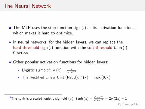
The MLP uses the step function sign (.) as its activation functions,which makes it hard to optimize.
In neural networks, for the hidden layers, we can replace thehard-threshold sign (.) function with the soft-threshold tanh (.)function.
Other popular activation functions for hidden layers:I Logistic sigmoid5: σ (x) = 1
1+e−x
I The Rectified Linear Unit (ReLU): f (x) = max (0, x)
5The tanh is a scaled logistic sigmoid (σ): tanh (x) = ex−e−x
ex +e−x = 2σ (2x)− 1© Jiaming Mao

The Neural Network
e-CHAPT
ER
e-7. Neural Networks 7.1. The Multi-layer Perceptron (MLP)
When θ(s) = sign(s), learning the weights was already a hard combinatorialproblem and had a variety of algorithms, including the pocket algorithm, forfitting data (Chapter 3). The combinatorial optimization problem is evenharder with the MLP, for the same reason, namely that the sign(·) function isnot smooth; a smooth, differentiable approximation to sign(·) will allow us touse analytic methods, rather than purely combinatorial methods, to find theoptimal weights. We therefore approximate, or ‘soften’ the sign(·) function byusing the tanh(·) function. The MLP is sometimes called a (hard) thresholdneural network because the transformation function is a hard threshold at zero.
linear
sign
tanh
Here, we choose θ(x) = tanh(x) which is in-between linear and the hard threshold: nearlylinear for x ≈ 0 and nearly ±1 for |x| large. Thetanh(·) function is another example of a sigmoid(because its shape looks like a flattened out ‘s’),related to the sigmoid we used for logistic regres-sion.2 Such networks are called sigmoidal neu-ral networks. Just as we could use the weightslearned from linear regression for classification, we could use weights learnedusing the sigmoidal neural network with tanh(·) activation function for classi-fication by replacing the output activation function with sign(·).
Exercise 7.5Given w1 and ϵ > 0, find w2 such that |sign(wt
1xn)− tanh(wt2xn)| ≤ ϵ
for xn ∈ D. [Hint: For large enough α, sign(x) ≈ tanh(αx).]
w
Ein
signtanh
The previous example shows that thesign(·) function can be closely approxi-mated by the tanh(·) function. A concreteillustration of this is shown in the figureto the right. The figure shows how thein-sample error Ein varies with one of theweights in w on an example problem forthe perceptron (blue curve) as comparedto the sigmoidal version (red curve). Thesigmoidal approximation captures the gen-eral shape of the error, so that if we minimize the sigmoidal in-sample error,we get a good approximation to minimizing the in-sample classification error.
2In logistic regression, we used the sigmoid because we wanted a probability as the output.Here, we use the ‘soft’ tanh(·) because we want a friendly objective function to optimize.
c⃝ AML Abu-Mostafa, Magdon-Ismail, Lin: Jan-2015 e-Chap:7–6
394 Neural Networks
-10 -5 0 5 10
0.0
0.5
1.0
1/(1
+e−
v)
v
FIGURE 11.3. Plot of the sigmoid function σ(v) = 1/(1+exp(−v)) (red curve),commonly used in the hidden layer of a neural network. Included are σ(sv) fors = 1
2(blue curve) and s = 10 (purple curve). The scale parameter s controls
the activation rate, and we can see that large s amounts to a hard activation atv = 0. Note that σ(s(v − v0)) shifts the activation threshold from 0 to v0.
Notice that if σ is the identity function, then the entire model collapsesto a linear model in the inputs. Hence a neural network can be thought ofas a nonlinear generalization of the linear model, both for regression andclassification. By introducing the nonlinear transformation σ, it greatlyenlarges the class of linear models. In Figure 11.3 we see that the rate ofactivation of the sigmoid depends on the norm of αm, and if ∥αm∥ is verysmall, the unit will indeed be operating in the linear part of its activationfunction.
Notice also that the neural network model with one hidden layer hasexactly the same form as the projection pursuit model described above.The difference is that the PPR model uses nonparametric functions gm(v),while the neural network uses a far simpler function based on σ(v), withthree free parameters in its argument. In detail, viewing the neural networkmodel as a PPR model, we identify
gm(ωTmX) = βmσ(α0m + αT
mX)
= βmσ(α0m + ∥αm∥(ωTmX)), (11.7)
where ωm = αm/∥αm∥ is the mth unit-vector. Since σβ,α0,s(v) = βσ(α0 +sv) has lower complexity than a more general nonparametric g(v), it is notsurprising that a neural network might use 20 or 100 such functions, whilethe PPR model typically uses fewer terms (M = 5 or 10, for example).
Finally, we note that the name “neural networks” derives from the factthat they were first developed as models for the human brain. Each unitrepresents a neuron, and the connections (links in Figure 11.2) representsynapses. In early models, the neurons fired when the total signal passed tothat unit exceeded a certain threshold. In the model above, this corresponds
Left: the tanh activation function. Note that for small x , tanh (x) ≈ x .Right: tanh (wx) for w = 0.5 (blue), w = 1 (red), and w = 10 (purple)
© Jiaming Mao

The Neural Network
For regression, the output layer typically contains a single unit6, withthe activation function being the identity function f (x) = x and theerror measure being the sum of squares error.
For binary classification, the output layer contains a single unit. Wecan choose the activation function to be the logistic sigmoid, with theerror measure being the binomial cross-entropy error.
For K−class multiclass classification, the output layer would containK units. We can choose the activation function to be the softmaxfunction, with the corresponding multinomial cross-entropy error7.
6It is also possible for have multiple output units for multiple quantitative responsesas in multivariate regressions.
7Alternatively, using a one-versus-all approach, we can choose the activation functionto be the logistic sigmoid and let the y be coded as a K−dimensional vector:y = [y1, . . . , yK ]′, where yj ∈ {0, 1} , j ∈ {1, . . . ,K}.
© Jiaming Mao

5.1. Feed-forward Network Functions 231
Figure 5.3 Illustration of the ca-pability of a multilayer perceptronto approximate four different func-tions comprising (a) f(x) = x2, (b)f(x) = sin(x), (c), f(x) = |x|,and (d) f(x) = H(x) where H(x)is the Heaviside step function. Ineach case, N = 50 data points,shown as blue dots, have been sam-pled uniformly in x over the interval(−1, 1) and the corresponding val-ues of f(x) evaluated. These datapoints are then used to train a two-layer network having 3 hidden unitswith ‘tanh’ activation functions andlinear output units. The resultingnetwork functions are shown by thered curves, and the outputs of thethree hidden units are shown by thethree dashed curves.
(a) (b)
(c) (d)
will show that there exist effective solutions to this problem based on both maximumlikelihood and Bayesian approaches.
The capability of a two-layer network to model a broad range of functions isillustrated in Figure 5.3. This figure also shows how individual hidden units workcollaboratively to approximate the final function. The role of hidden units in a simpleclassification problem is illustrated in Figure 5.4 using the synthetic classificationdata set described in Appendix A.
5.1.1 Weight-space symmetriesOne property of feed-forward networks, which will play a role when we consider
Bayesian model comparison, is that multiple distinct choices for the weight vectorw can all give rise to the same mapping function from inputs to outputs (Chen et al.,1993). Consider a two-layer network of the form shown in Figure 5.1 with M hiddenunits having ‘tanh’ activation functions and full connectivity in both layers. If wechange the sign of all of the weights and the bias feeding into a particular hiddenunit, then, for a given input pattern, the sign of the activation of the hidden unit willbe reversed, because ‘tanh’ is an odd function, so that tanh(−a) = − tanh(a). Thistransformation can be exactly compensated by changing the sign of all of the weightsleading out of that hidden unit. Thus, by changing the signs of a particular group ofweights (and a bias), the input–output mapping function represented by the networkis unchanged, and so we have found two different weight vectors that give rise tothe same mapping function. For M hidden units, there will be M such ‘sign-flip’
Approximation of (a) f (x) = x2; (b) f (x) = sin (x); (c) f (x) = |x |; (d)f (x) = sign (x) using a two-layer neural network with three hidden units and alinear output. Blue dots: data from the underlying function; Red line: neural
network output; Dashed lines: outputs of the three hidden units.© Jiaming Mao

Biological Inspiration
© Jiaming Mao

Biological Inspiration
© Jiaming Mao

Estimation
Let w ={w (1), . . . ,w (L)
}. A neural network model is H = {h (x ;w)}.
The training error for a neural network is
Ein (w) = 1N
N∑n=1
` (h (xn;w) , yn)
, where ` is the appropriate loss function.
To estimate w , we need to compute ∇Ein (w), i.e., for each data point(xn, yn), we need to compute
∂en (w)∂w (`)
ij∀i , j , ` (1)
, where en (w) = ` (h (xn;w) , yn).
© Jiaming Mao

Estimation
An efficient way to compute (1):
∂en (w)∂w (`)
ij= ∂en (w)
∂s(`)j×∂s(`)
j
∂w (`)ij
= x (`−1)i δ
(`)j
, where δ(`)j ≡
∂en(w)∂s(`)
j.
© Jiaming Mao

Forward Propagation
We can calculate x (`) =[1, x (`)
1 , . . . , x (`)d(`)
]′based on x (`−1):
s(`) =(W (`)
)′x (`−1)
x (`) =[
1θ(s(`)) ]
Therefore, starting with x (0) = xn, we can calculate x (`) for all ` as follows:
xn = x (0) W (1)−→ s(1) θ−→ x (1) −→ · · · s(L) θ−→ x (L) = h (xn)
This is called forward propagation.
© Jiaming Mao

Forward Propagation
e-CHAPT
ER
e-7. Neural Networks 7.2. Neural Networks
Forward propagation to compute h(x):1: x(0) ← x [Initialization]2: for ℓ = 1 to L [Forward Propagation]do3: s(ℓ) ← (W(ℓ))tx(ℓ−1)
4: x(ℓ) ←!
1
θ(s(ℓ))
"
5: h(x) = x(L) [Output]
x(ℓ)
θ(·)
θ(·)
x(ℓ−1)
W(ℓ)
+
+
s(ℓ)...
layer ℓlayer (ℓ− 1)
11
...
After forward propagation, the output vector x(ℓ) at every layer l = 0, . . . , Lhas been computed.
Exercise 7.6Let V and Q be the number of nodes and weights in the neural network,
V =L!
ℓ=0
d(ℓ), Q =L!
ℓ=1
d(ℓ)(d(ℓ−1) + 1).
In terms of V and Q, how many computations are made in forward propa-gation (additions, multiplications and evaluations of θ).
[Answer: O(Q) multiplications and additions, and O(V ) θ-evaluations.]
If we want to compute Ein, all we need is h(xn) and yn. For the sum ofsquares,
Ein(w) =1
N
N#
n=1
(h(xn;w)− yn)2
=1
N
N#
n=1
(x(L)n − yn)2.
c⃝ AML Abu-Mostafa, Magdon-Ismail, Lin: Jan-2015 e-Chap:7–10
© Jiaming Mao

Backward Propagation
δ(l) =[δ
(`)1 , . . . , δ
(`)d(`)
]′can be calculated
from δ(l+1).
Starting from the output layer, assum-ing single unit output, the identity acti-vation function, and sum-of-squares error,we have:
δ(L) = ∂en (w)∂s(L)
=∂(θ(s(L)
)− yn
)2
∂s(L)
= 2(x (L) − yn
)
© Jiaming Mao

Backward Propagation
For ` < L,
δ(l−1)i = ∂en (w)
∂s(`−1)j
=d(`)∑j=1
∂en (w)∂s(`)
j×
∂s(`)j
∂x (`−1)i
× ∂x (`−1)i
∂s(`−1)i
=d(`)∑j=1
δ(`)j × w (`)
ij × θ′(s(`−1)i
), where, for θ (.) = tanh (.), we havetanh′
(s(`−1)i
)= 1−
[tanh
(s(`−1)i
)]2= 1−
(x (`−1)
i
)2.
© Jiaming Mao

Backward PropagationTherefore, starting with δ(L), we can calculate δ(`) for all `:
δ(1) ←− δ(2) · · · ←− δ(L−1) ←− δ(L)
This is called backward propagation.
e-CHAPT
ER
e-7. Neural Networks 7.2. Neural Networks
δ(ℓ)
+
+× θ′(s(ℓ))
... W(ℓ+1)δ(ℓ+1)
...
layer ℓ layer (ℓ + 1)
1 1
As you can see in the figure, the neural network is slightly modified only inthat we have changed the transformation function for the nodes. In forwardpropagation, the transformation was the sigmoid θ(·). In backpropagation,the transformation is multiplication by θ′(s(ℓ)), where s(ℓ) is the input to thenode. So the transformation function is now different for each node, andit depends on the input to the node, which depends on x. This input wascomputed in the forward propagation. For the tanh(·) transformation function,tanh′(s(ℓ)) = 1−tanh2(s(ℓ)) = 1−x(ℓ)⊗x(ℓ), where ⊗ denotes component-wisemultiplication.
In the figure, layer (ℓ+1) outputs (backwards) the sensitivity vector δ(ℓ+1),which gets multiplied by the weights W(ℓ+1), summed and passed into thenodes in layer ℓ. Nodes in layer ℓ multiply by θ′(s(ℓ)) to get δ(ℓ). Using ⊗, ashorthand notation for this backpropagation step is:
δ(ℓ) = θ′(s(ℓ))⊗ [W(ℓ+1)δ(ℓ+1)!d(ℓ)
1, (7.5)
where the vector"W(ℓ+1)δ(ℓ+1)
!d(ℓ)
1contains components 1, . . . , d(ℓ) of the vec-
tor W(ℓ+1)δ(ℓ+1) (excluding the bias component which has index 0). This for-mula is not surprising. The sensitivity of e to inputs of layer ℓ is proportionalto the slope of the activation function in layer ℓ (bigger slope means a smallchange in s(ℓ) will have a larger effect on x(ℓ)), the size of the weights goingout of the layer (bigger weights mean a small change in s(ℓ) will have moreimpact on s(ℓ+1)) and the sensitivity in the next layer (a change in layer ℓaffects the inputs to layer ℓ + 1, so if e is more sensitive to layer ℓ + 1, then itwill also be more sensitive to layer ℓ).
We will derive this backward recursion later. For now, observe that if weknow δ(ℓ+1), then you can get δ(ℓ). We use δ(L) to seed the backward process,and we can get that explicitly because e = (x(L) − y)2 = (θ(s(L)) − y)2.
c⃝ AML Abu-Mostafa, Magdon-Ismail, Lin: Jan-2015 e-Chap:7–13
© Jiaming Mao

Gradient Descent
Forward and backward propagation provide an efficient method tocompute ∇Ein (w). We can then search for the optimal w∗ thatminimizes Ein (w) using optimization techniques such as batch andstochastic gradient descent.
In practice, there is quite an art in training neural networks, as theoptimization problem is nonconvex with many local minima.
© Jiaming Mao

Gradient Descent
Gradient Descent (Batch)
Initialize all weights w ={w (`)
ij
}at random.
For t = 0, 1, 2, . . ., do until the convergence of wFor each data point (xn, yn), n = 1, . . . ,N, do
Compute x (`) for ` = 1, . . . , L (forward propagation)Compute δ(`) for ` = L, . . . , 1 (backward propagation)Compute ∇en (w) : ∂en (w)
/∂w (`)
ij = x (`−1)i δ
(`)j
Compute ∇Ein (w) = 1N∑N
n=1∇en (w)Update w : w ←− w − η∇Ein (w)
© Jiaming Mao

Gradient Descent
Stochastic Gradient Descent (SGD)
Initialize all weights w ={w (`)
ij
}at random.
For t = 0, 1, 2, . . ., do until the convergence of wFor each data point (xn, yn), n = 1, . . . ,N, do
Compute x (`) for ` = 1, . . . , L (forward propagation)Compute δ(`) for ` = L, . . . , 1 (backward propagation)Compute ∇en (w) : ∂en (w)
/∂w (`)
ij = x (`−1)i δ
(`)j
Update w : w ←− w − η∇en (w)
© Jiaming Mao

Gradient Descent
e-CHAPT
ER
e-7. Neural Networks 7.2. Neural Networks
SGD
Gradient Descent
log10(iteration)
log10(e
rror
)
0 2 4 6
-4
-3
-2
-1
0In Chapter 3, we discussed stochas-
tic gradient descent (SGD) as a moreefficient alternative to the batch mode.Rather than wait for the aggregate gra-dient G(ℓ) at the end of the iteration, oneimmediately updates the weights as eachdata point is sequentially processed usingthe single point gradient in step 7 of thealgorithm: W(ℓ) = W(ℓ) − ηG(ℓ)(xn). Inthis sequential version, you still run a for-ward and backward propagation for eachdata point, but make N updates to the weights. A comparison of batch gra-dient descent with SGD is shown to the right. We used 500 training examplesfrom the digits data and a 2-layer neural network with 5 hidden units andlearning rate η = 0.01. The SGD curve is erratic because one is not minimiz-ing the total error at each iteration, but the error on a specific data point.One method to dampen this erratic behavior is to decrease the learning rateas the minimization proceeds.
The speed at which you minimize Ein can depend heavily on the optimiza-tion algorithm you use. SGD appears significantly better than plain vanillagradient descent, but we can do much better – even SGD is not very efficient.In Section 7.5, we discuss some other powerful methods (for example, conju-gate gradients) that can significantly improve upon gradient descent and SGD,by making more effective use of the gradient.
Initialization and Termination. Choosing the initial weights and decid-ing when to stop the gradient descent can be tricky, as compared with logisticregression, because the in-sample error is not convex anymore. From Exer-cise 7.7, if the weights are initialized too large so that tanh(wtxn) ≈ ±1,then the gradient will be close to zero and the algorithm won’t get any-where. This is especially a problem if you happen to initialize the weightsto the wrong sign. It is usually best to initialize the weights to small ran-dom values where tanh(wtxn) ≈ 0 so that the algorithm has the flexibility tomove the weights easily to fit the data. One good choice is to initialize usingGaussian random weights, wi ∼ N(0, σ2
w) where σ2w is small. But how small
should σ2w be? A simple heuristic is that we want |wtxn|2 to be small. Since
Ew
!|wtxn|2
"= σ2
w∥xn∥2, we should choose σ2w so that σ2
w · maxn ∥xn∥2 ≪ 1.
Exercise 7.9What can go wrong if you just initialize all the weights to exactly zero?
c⃝ AML Abu-Mostafa, Magdon-Ismail, Lin: Jan-2015 e-Chap:7–18
© Jiaming Mao

Training Your Neural Network: Initialization
To train a neural network, it is best to standardize all inputs to have meanzero and standard deviation one. The starting values for w are usuallychosen to be random values near zero, e.g. wi ∼ N
(0, σ2
w), where σw is
small.
Use of exact zero weights leads to zero derivatives and perfectsymmetry, and the algorithm never moves.
Starting with large weights so that tanh (w ′x) ≈ ±1 also leads toclose to zero derivatives.
Hence the initial values for w should be random values near zero sothat the model starts out nearly linear, and becomes nonlinear as theweights increase.
© Jiaming Mao

Training Your Neural Network: Regularization
The neural network model is in essence a hyper-parametrized nonlinearmodel that can contain an arbitrary number of parameters to approximateany smooth functions.
To avoid overfitting, we typically do not want the global minimizer ofEin (w). Instead, some regularization is needed, which can be achieved byadding a penalty term. For example, we can minimize the followingaugmented error:
Eaug (w) = Ein (w) + λ ‖w‖2 (2)
The L2 regularizer (2) is also called weight decay in the context of neuralnetworks. The tuning parameter λ is typically selected by cross validation.
© Jiaming Mao

Training Your Neural Network: Regularization
Alternatively, regularization can be achieved by early stopping: train themodel only for a while, and stop well before we approach the globalminimum.
Since we initialize weights near zero, early stopping has the effect ofachieving smaller weights, similar to weight decay.
I Equivalently, it has the effect of shrinking the final model toward alinear model.
A validation set is used for determining when to stop.
© Jiaming Mao

Training Your Neural Network: Regularization
e-CHAPT
ER
e-7. Neural Networks 7.4. Regularization and Validation
iteration, t
log10(e
rror
)
t∗Ein
Etest
102 103 104
-1.8
-1.4
-1
-0.6
-0.2
The curves reinforce our theoretical discussion: the test error initially decreasesas the approximation gain overcomes the worse generalization error bar; then,the test error increases as the generalization error bar begins to dominate theapproximation gain, and overfitting becomes a serious problem. !
In the previous example, despite using a parsimonious neural network withjust a single hidden node, overfitting was an issue because the data are noisyand the target function is complex, so both stochastic and deterministic noiseare significant. We need to regularize.
w0
wt∗
contour of constant Ein
In the example, it is better to stop earlyat t∗ and constrain the learning to thesmaller hypothesis set Ht∗ . In this sense,early stopping is a form of regularization.Early stopping is related to weight decay,as illustrated to the right. You initialize w0
near zero; if you stop early at wt∗ you havestopped at weights closer to w0, i.e., smallerweights. Early stopping indirectly achievessmaller weights, which is what weight decaydirectly achieves. To determine when to stoptraining, use a validation set to monitor thevalidation error at iteration t as you minimize the training-set error. Reportthe weights wt∗ that have minimum validation error when you are done train-ing.
After selecting t∗, it is tempting to use all the data to train for t∗ iterations.Unfortunately, adding back the validation data and training for t∗ iterationscan lead to a completely different set of weights. The validation estimate ofperformance only holds for wt∗ (the weights you should output). This appearsto go against the wisdom of the decreasing learning curve from Chapter 4: ifyou learn with more data, you get a better final hypothesis.10
10Using all the data to train to an in-sample error of Etrain(wt∗ ) is also not recommended.Further, an in-sample error of Etrain(wt∗ ) may not even be achievable with all the data.
c⃝ AML Abu-Mostafa, Magdon-Ismail, Lin: Jan-2015 e-Chap:7–26
Early Stopping
© Jiaming Mao

Training Your Neural Network: RegularizationWeight Decay with Digits Data
No Weight Decay Weight Decay, λ = 0.01
Average Intensity
Sym
met
ry
Average Intensity
Sym
met
ry
c⃝ AML Creator: Malik Magdon-Ismail Neural Networks and Overfitting: 7 /15 Early Stopping −→
Weight Decay
© Jiaming Mao

Training Your Neural Network: Regularization
e-CHAPT
ER
e-7. Neural Networks 7.5. Beefing Up Gradient Descent
iteration, t
log10(e
rror
)
Ein
Eval
t∗
102 103 104 105 106
-1.6
-1.4
-1.2
-1
Average Intensity
Sym
met
ry(a) Training dynamics (b) Final hypothesis
Figure 7.3: Early stopping with 500 examples from the digits data. (a)Training and validation errors for gradient descent with a training set ofsize 450 and validation set of size 50. (b) The ‘regularized’ final hypothesisobtained by early stopping at t∗, the minimum validation error.
Etrain Eval Ein EoutNo Regularization – – 0.2% 3.1%Weight Decay – – 1.0% 2.1%Early Stopping 1.1% 2.0% 1.2% 2.0%
7.5 Beefing Up Gradient DescentGradient descent is a simple method to minimize Ein that has problems con-verging, especially with flat error surfaces. One solution is to minimize afriendlier error instead, which is why training with a linear output node helps.Rather than change the error measure, there is plenty of room to improvethe algorithm itself. Gradient descent takes a step of size η in the negativegradient direction. How should we determine η and is the negative gradientthe best direction in which to move?
Exercise 7.14Consider the error function E(w) = (w−w∗)tQ(w−w∗), where Q is anarbitrary positive definite matrix. Set w = 0.
Show that the gradient ∇E(w) = −Qw∗. What weights minimize E(w).Does gradient descent move you in the direction of these optimal weights?
Reconcile your answer with the claim in Chapter 3 that the gradient is thebest direction in which to take a step. [Hint: How big was the step?]
The previous exercise shows that the negative gradient is not necessarily thebest direction for a large step, and we would like to take larger steps to increase
c⃝ AML Abu-Mostafa, Magdon-Ismail, Lin: Jan-2015 e-Chap:7–29
Early Stopping
© Jiaming Mao

Training Your Neural Network: Hidden Units
One can control the complexity of a model by regularization or bylimiting the number of hidden units.
In practice, regularization strength – rather than the number ofneurons – is the preferred way to control overfitting. It it better tohave a reasonably large number of units and train them withregularization.
© Jiaming Mao

Simulation
# Simulationn = 1000x = matrix(rnorm(n*2),ncol=2)x[1:n/2,] = x[1:n/2,] + 2x[(n/2+1):(n/4*3),] = x[(n/2+1):(n/4*3),] - 2y = c(rep(1,(n/4*3)),rep(2,(n/4)))
# Create training and test setsdata = data.frame(x1=x[,1],x2=x[,2],y=as.factor(y))train = sample(n,n*0.4)data_train = data[train,]data_test = data[-train,]
© Jiaming Mao

Simulation
●
●
●
●
●
● ●
●
●●
●●
●
●
●
●
●
●
●
●
●
●
●
●
●
●
●
●●
●
●
●●
●
●
●
●
●
●
●
●
●
●
●
●
●
●
●
●
●
●●
●
●
●●
●
●
●
●
●
●
●
●
●
●
●
● ●
●
●
●
●
● ●
●
●
●
●
●
●
●
●
●
●
●
●
●
●
●
●
●
●
●
●
●●
●
●
●
●
●
●
●
●
●
●
●
●
●
●
●
●
●●
●
●
●
●
●
●
●
●
●
●
●
●
●
●
●
●
●
●
●
●
●
●
●
●
●
●
●
●
●
●
●●
●
●
●●
●
●
●●
●
● ● ●
●
●
●
●
●
●
●
●
●
●
●
●
●
●
●●
●
●
●
●
●
●●
●●
●
●●
●●
●
●
●
●
●
●
● ●
●
●
●
●
●
●
●
●●
●
●
●●
●
●
●
●
●
●
●
●
●
●
●
●
●
●
●
●
●
●
●
●
●
●
●
●
●
●
●
●
●
●
●
●
●
●
●
●
●
●
●
●
●
●
●
●
●
●
●
●
●
●
●
●●
● ●
●
●
●
●
●
●
●
●
●
●
●
●
●
●●
●
●
●
●
●
●
●
●
●
●●
●
●
●
●
●
●
●●
●
●
●
●
●
●
●
●
●
●
●
●
●
●
●
●
●
●
●
●
● ●
●
●
●
●
●
●
●
●
●
●
●
●
●
●
●
●
●
●
●
●
●
●
●
●
●
●
●
●
●●
●
●
●●
●
●
●
●
●● ●
●
●
●
●
●
●
●
●
●
●
●
●
●
●
●
●
●
●
●
●
●
●
●
● ●
●●
●
●
●
●
●
●
●●
●
●●
−4 −2 0 2 4
−4
−2
02
4
x1
x2
© Jiaming Mao

Simulation
# Here we fit a single-hidden-layer network with 10 hidden units# and choose the weight decay parameter by cross-validationrequire(caret)fit = train(y ~.,data=data_train,method="nnet",
preProcess=c("center","scale"),tuneGrid=expand.grid(size=1:20,
decay=c(0.001,0.01,0.1,1)),trControl=trainControl(method="repeatedcv",repeats=3))
fit$bestTune
## size decay## 3 10 0.1
# test errytrue = data_test[,"y"]yhat = predict(fit,data_test) # predict using fit$bestTune1-mean(yhat==ytrue)
## [1] 0.1033333© Jiaming Mao

Simulation
−4 −2 0 2 4
−4
−2
02
4
Neural Networks
© Jiaming Mao

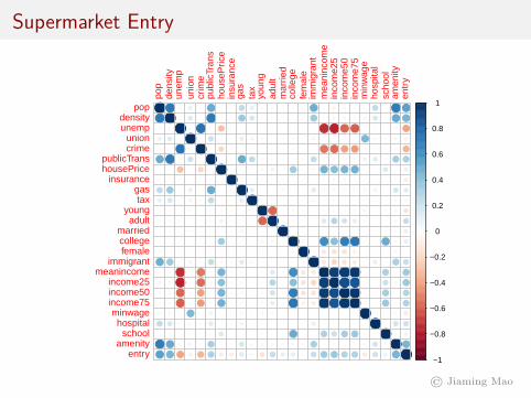
Supermarket Entry
Supermarket entry in geographical markets. For each market, data include:
total populationpopulation densityaverage incomepercentage population with college degreeminimum wageunemployment ratecrime rateetc.
© Jiaming Mao

Supermarket Entry
# read datadata = read.csv("supermarket_entry.csv")data[,1:24] = scale(data[,1:24]) # center & scale datadata$entry = as.factor(data$entry)
# create training and test setsrequire(caret)train = createDataPartition(data$entry,p=0.5,list=F)data_train = data[train,]data_test = data[-train,]
© Jiaming Mao
Supermarket Entry
●●
●
●
●
●●
●
●
●
●
●
●
●
●
●●
●
●
●
●
●
●
●●
●●
●
●
●
●●
●
●
●
●
●
●
●
●
●●
●
●
●
●
●
●
●●
●
●
●●
●●
●
●
●
●
●
●
●
●
●
●
●●●●
●
●
●
●
●
●
●
●
●●
●
●
●
●
●
●
●
●
●
●
●
●
●
●
●
●●
●
●
●
●
●
●●
●●
●
●
●
●
●
●
●
●
●
●
●●●
●●
●
●
●
●
●
●●
●
●
●●
●
●●
●
●
●
●
●
●
●
●
●
●
●
●
●
●
●
●
●
●●
●
●
●●
●
●
●
●
●
●●
●
●●
●●
●
●
●
●
●
●
●
●
●
●
●
●
●●
●
●
●
●
●
●
●
●
●
●
●
●
●
●
●
●
●
●●
●
●
●●
●
●●
●
●
●
●
●
●
●
●
●
●
●
●
●
●
●
●
●
●
●
●
●
●
●
●
●●
●
●
●
●
●
●
●
●
●
●
●
●
●
●
●
●
●
●
●
●
●
●
●
●
●●
●
●
●
●
●
●
●
●
●
●
●
●
●
●
●
●
●
●
●
●
●
●
●
●●
●
●
●
●
●
●
●
●
●
●
●
●
●
●
●
●
●
●
●
●
●
●
●
●
●
●●
●
●
●
●
●
●
●
●
●
●
●
●
●
●
●
●
●
●●
●
●
●
●
●
●●
●
●●
●●
●
●
●●
●
●
●
●
●
●
●
●
●
●
●
●
●
●
●
●●
●
●
●
●
●
●
●
●
●
●●
●
●
●
●
●
●
●
●
●
●
●
●
●
●●
●
●
●
●
●
●
●
●
●
●
●●
●●
●●
●
●
●
●
●
●●
●
●●●●
●
●
●●
●
●
●
●●
●●
●●
●
●
●
●●
●●
●
●●●●
●
●
●
●
●
●
●
●●
●●
●●
●
●
●
●
●
●●
●
●●●●
●
●
●●
●
●
●
●●
●●
●●
●
●
●
●
●
●●
●
●●●●
●
●
●●
●
●
●
●
●●
●
●
●
●
●
●
●
●
●
●
●
●
●
●
●
●●
●
●
●
●
●
●
●
●
●
●
●
●
●
●
●
●
●
●
●
●
●
●
●
●
●●
●
●
●
●
●
●
●
●
●
●
●
●
●
●
●
●●
●
●
●
●
●●
●
●●
●
●●
●
●
●
●●
●
●
●
●
●
●
●
●
●●
●
●
●
●
●
●
●●
●●●●
●
●
●
●
●
●
●
●
●
●
●
●
●
●
●
●
●
●
●
●
● −1
−0.8
−0.6
−0.4
−0.2
0
0.2
0.4
0.6
0.8
1
pop
dens
ityun
emp
unio
ncr
ime
publ
icTr
ans
hous
ePric
ein
sura
nce
gas
tax
youn
gad
ult
mar
ried
colle
gefe
mal
eim
mig
rant
mea
ninc
ome
inco
me2
5in
com
e50
inco
me7
5m
inw
age
hosp
ital
scho
olam
enity
entr
y
popdensityunemp
unioncrime
publicTranshousePrice
insurancegastax
youngadult
marriedcollegefemale
immigrantmeanincome
income25income50income75minwagehospital
schoolamenity
entry
© Jiaming Mao

Supermarket Entry
######################## Logistic Regression ########################require(AER)fit = glm(entry~.,data_train,family="binomial")results = coeftest(fit)results[1:10,]
## Estimate Std. Error z value Pr(>|z|)## (Intercept) -2.453152189 0.1967120 -12.47077924 1.077670e-35## pop 2.926116034 0.2739735 10.68028881 1.258794e-26## density 1.772984978 0.2275741 7.79080418 6.658404e-15## unemp -2.765055539 0.5330852 -5.18689228 2.138323e-07## union -1.101124570 0.1531317 -7.19070145 6.445929e-13## crime -0.976543245 0.1792566 -5.44773919 5.101409e-08## publicTrans 0.259851907 0.1745623 1.48859149 1.365950e-01## housePrice -0.737637260 0.1415481 -5.21121131 1.876116e-07## insurance -1.047932648 0.1389732 -7.54053789 4.680369e-14## gas 0.002968719 0.1322816 0.02244242 9.820950e-01
© Jiaming Mao

Supermarket Entry
results[11:25,]
## Estimate Std. Error z value Pr(>|z|)## tax -0.9355652 0.1379065 -6.7840523 1.168510e-11## young -0.3732518 0.1916235 -1.9478395 5.143417e-02## adult 1.6714084 0.2659985 6.2835250 3.309811e-10## married 1.2394382 0.1467281 8.4471788 2.984265e-17## college 1.4075509 0.4098684 3.4341534 5.944078e-04## female -0.2281599 0.1520545 -1.5005139 1.334813e-01## immigrant -0.1331635 0.1748719 -0.7614918 4.463634e-01## meanincome 1.0099997 0.9532922 1.0594860 2.893785e-01## income25 1.6291830 0.5389211 3.0230454 2.502447e-03## income50 -0.7924468 0.5308270 -1.4928531 1.354756e-01## income75 -1.7747426 0.7851714 -2.2603251 2.380108e-02## minwage -0.9216894 0.1454276 -6.3377867 2.330892e-10## hospital 0.6793887 0.1350251 5.0315743 4.864686e-07## school 0.6074254 0.1415092 4.2924806 1.766880e-05## amenity 0.8117051 0.1674314 4.8479857 1.247214e-06
© Jiaming Mao

Supermarket Entry
# test errytrue = data_test$entryphat = predict(fit,data_test,type="response")yhat = as.numeric(phat > 0.5)table(ytrue,yhat)
## yhat## ytrue 0 1## 0 907 64## 1 79 520
1-mean(yhat==ytrue)
## [1] 0.0910828
© Jiaming Mao

Supermarket Entry
######################## Classification Tree ########################require(rpart)fit = rpart(entry~.,data_train)
# test erryhat = predict(fit,data_test,type="class")1-mean(yhat==ytrue)
## [1] 0.1656051
© Jiaming Mao

Supermarket Entry
################## Random Forest ##################require(randomForest)fit = randomForest(entry~.,data=data_train,mtry=6) # mtry selected by cv
# test erryhat = predict(fit,data_test)1-mean(yhat==ytrue)
## [1] 0.1031847
© Jiaming Mao

Supermarket Entry
############# Boosting #############require(gbm)data_boost = transform(data_train,entry=as.numeric(entry)-1)fit = gbm(entry~.,data=data_boost,distribution="adaboost",
n.trees=2000,interaction.depth=10,shrinkage = 0.01) # parameters selected by cv
# test errphat = predict(fit,data_test,n.trees=2000,type="response")yhat = as.numeric(phat>0.5)1-mean(yhat==ytrue)
## [1] 0.06305732
© Jiaming Mao

Supermarket Entry
######## SVM ########require(e1071)fit= svm(entry~.,data_train,kernel="radial", # RBF kernel
scale=F,gamma=0.01,cost=30) # parameters selected by cv
# test erryhat = predict(fit,data_test,type="class")1-mean(yhat==ytrue)
## [1] 0.07197452
© Jiaming Mao

Supermarket Entry
################### Neural Network #################### Fit a single-hidden-layer networkrequire(nnet)fit = nnet(entry ~.,data_train,maxit=10000,
size=10,decay=0.1) # parameters selected by cv
# test erryhat = predict(fit,data_test,type="class")1-mean(yhat==ytrue)
## [1] 0.04394904
© Jiaming Mao

Supermarket Entry
amenityschoolhospitalminwageincome75income50income25meanincomeimmigrantfemalecollegemarriedadultyoungtaxgasinsurancehousePricepublicTranscrimeunionunempdensitypop
entry
1 1
© Jiaming Mao
Supermarket Entry
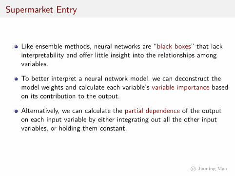
Like ensemble methods, neural networks are “black boxes” that lackinterpretability and offer little insight into the relationships amongvariables.
To better interpret a neural network model, we can deconstruct themodel weights and calculate each variable’s variable importance basedon its contribution to the output.
Alternatively, we can calculate the partial dependence of the outputon each input variable by either integrating out all the other inputvariables, or holding them constant.
© Jiaming Mao

Supermarket Entry
unempcrime
insuranceunion
taxhousePrice
minwageyoung
collegeincome75
gaspublicTrans
femaleimmigrant
hospitalincome50
schoolamenitymarried
adultincome25
densitymeanincome
pop
−20 0 20 40Importance
© Jiaming Mao
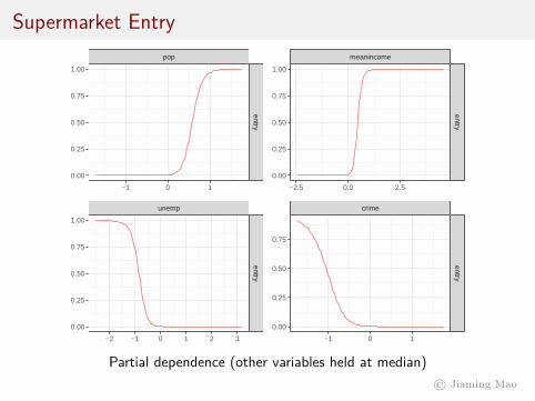
Supermarket Entrypop
entry
−1 0 1
0.00
0.25
0.50
0.75
1.00
meanincome
entry
−2.5 0.0 2.5
0.00
0.25
0.50
0.75
1.00
unemp
entry
−2 −1 0 1 2 3
0.00
0.25
0.50
0.75
1.00
crime
entry
−1 0 1
0.00
0.25
0.50
0.75
Partial dependence (other variables held at median)© Jiaming Mao

The Neural Network: Discussion
Consider a neural network with a single hidden layer, which implements afunction of the form
h (x) = f(β0 +
M∑m=1
βmθ(γ′mx
))(3)
, where θ (.) is the hidden layer activation function and f (.) is the outputlayer activation function. There are M + 1 number of units in the hiddenlayer. γm are the weights going into the mth unit of the hidden layer, andβ are the weights going into the output layer.
© Jiaming Mao

The Neural Network: Discussion
(3) is equivalent in functional form to a linear model with featuretransform Φ and a nonlinear output transform f 8:
h (x) = f(β0 +
M∑m=1
βmφm (x))
(4)
, where Φ = (φ1, . . . , φM) are the basis functions.
8If f (.) is the identity function, then (4) is a linear basis function model.© Jiaming Mao

The Neural Network: Discussion
Difference between (3) and (4):
In (4), the basis functions φm are fixed before seeing the data.
In (3), θ (γ′mx) contains the parameters γm that are to be learnedfrom the data.
The θ (γ′mx)’s are therefore called tunable or adaptive basis functions9
that give the neural network much more flexibility to fit the data thanfixed basis functions.
9As in boosting© Jiaming Mao

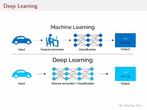
Feature Engineering vs. Feature Learning
Because in neural networks, neurons in hidden layers can be thoughtof as features that are learned from the data, neural networks can bethought of as enabling feature learning or representation learning.
In contrast, in “classical” machine learning, features are manuallyconstructed by human experts – a practice called featureengineering. Algorithms are then applied to find the mapping fromfeatures to output.
© Jiaming Mao

Deep Learning
Deep learning models are neural networks with many hidden layers. Thisallows the construction of hierarchical features and enables representationlearning with multiple levels of representation that correspond to multiplelevels of abstraction.
Shallow neurons represent low level features. Deep neurons representhigh level features.
More complex representations are expressed in terms of other, simplerrepresentations.
© Jiaming Mao
Deep Learning
© Jiaming Mao

Deep LearningNeural Networks as Feature LearningMulti-Layer Feature Learning
Taken from Yan LeCun’s deep learning tutorial
Shai Shalev-Shwartz (Hebrew U) IML Lecture 10 Neural Networks 28 / 31
© Jiaming Mao

Deep Learning
Deep networks are highly flexible and allow a wide variety ofarchitectures, which allow the incorporation of domain-specificknowledge (e.g., translational invariance in image recognition) intothe model.
Like parametric models, neural networks have specific parameters tolearn, but like nonparametric models, their complexity can grow withdata.
While “classical” nonparametric methods rely mainly on thesmoothness prior, deep neural nets impose a structure of hierarchicalrepresentation while incorporating domain-specific knowledge in orderto defeat the curse of dimensionality.
© Jiaming Mao
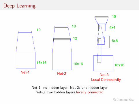
Deep Learning 11.7 Example: ZIP Code Data 405
16x16
8x8x2
16x16
10
4x4
4x4
8x8x2
10
Shared Weights Net-5Net-4
Net-1
4x4x4
Local Connectivity
1010
10
Net-3Net-2
8x812
16x1616x1616x16
FIGURE 11.10. Architecture of the five networks used in the ZIP code example.
phasize the effects. The examples were obtained by scanning some actualhand-drawn digits, and then generating additional images by random hor-izontal shifts. Details may be found in Le Cun (1989). There are 320 digitsin the training set, and 160 in the test set.
Five different networks were fit to the data:
Net-1: No hidden layer, equivalent to multinomial logistic regression.
Net-2: One hidden layer, 12 hidden units fully connected.
Net-3: Two hidden layers locally connected.
Net-4: Two hidden layers, locally connected with weight sharing.
Net-5: Two hidden layers, locally connected, two levels of weight sharing.
These are depicted in Figure 11.10. Net-1 for example has 256 inputs, oneeach for the 16×16 input pixels, and ten output units for each of the digits0–9. The predicted value f̂k(x) represents the estimated probability thatan image x has digit class k, for k = 0, 1, 2, . . . , 9.
Net-1: no hidden layer; Net-2: one hidden layerNet-3: two hidden layers locally connected
© Jiaming Mao

Deep Learning
11.7 Example: ZIP Code Data 405
16x16
8x8x2
16x16
10
4x4
4x4
8x8x2
10
Shared Weights Net-5Net-4
Net-1
4x4x4
Local Connectivity
1010
10
Net-3Net-2
8x812
16x1616x1616x16
FIGURE 11.10. Architecture of the five networks used in the ZIP code example.
phasize the effects. The examples were obtained by scanning some actualhand-drawn digits, and then generating additional images by random hor-izontal shifts. Details may be found in Le Cun (1989). There are 320 digitsin the training set, and 160 in the test set.
Five different networks were fit to the data:
Net-1: No hidden layer, equivalent to multinomial logistic regression.
Net-2: One hidden layer, 12 hidden units fully connected.
Net-3: Two hidden layers locally connected.
Net-4: Two hidden layers, locally connected with weight sharing.
Net-5: Two hidden layers, locally connected, two levels of weight sharing.
These are depicted in Figure 11.10. Net-1 for example has 256 inputs, oneeach for the 16×16 input pixels, and ten output units for each of the digits0–9. The predicted value f̂k(x) represents the estimated probability thatan image x has digit class k, for k = 0, 1, 2, . . . , 9.
Net-4: two hidden layers, locally connected with weight sharingNet-5: two hidden layers, locally connected, two levels of weight sharing
© Jiaming Mao

Deep LearningCHAPTER 1. INTRODUCTION
Input
Hand-
designed
program
Output
Input
Hand-
designed
features
Mapping from
features
Output
Input
Features
Mapping from
features
Output
Input
Simple
features
Mapping from
features
Output
Additional
layers of more
abstract
features
Rule-based
systems
Classic
machine
learning Representation
learning
Deep
learning
Figure 1.5: Flowcharts showing how the different parts of an AI system relate to each
other within different AI disciplines. Shaded boxes indicate components that are able to
learn from data.
10
© Jiaming Mao

Acknowledgement
Part of this lecture is adapted from the following sources:
Abu-Mostafa, Y. S., M. Magdon-Ismail, and H. Lin. 2012. Learningfrom Data. AMLBook.Bishop, C. M. 2011. Pattern Recognition and Machine Learning.Springer.Goodfellow, I., Y. Bengio, and A. Courville. 2016. Deep Learning.The MIT Press.Hastie, T., R. Tibshirani, and J. Friedmand. 2008. The Elements ofStatistical Learning (2nd ed.). Springer.
© Jiaming Mao
![Deep Parametric Continuous Convolutional Neural Networks€¦ · Graph Neural Networks: Graph neural networks (GNNs) [25] are generalizations of neural networks to graph structured](https://img.dokumen.tips/doc/110x75/5f7096c356401635d36dbe30/deep-parametric-continuous-convolutional-neural-networks-graph-neural-networks.jpg)