Embed Size (px)
Citation preview

Neural Networks for Acoustic Modelling part 2;Sequence discriminative training
Steve Renals
Automatic Speech Recognition – ASR Lecture 916 February 2017
ASR Lecture 9 Neural Networks for Acoustic Modelling part 2; Sequence discriminative training1

DNN Acoustic Models
ASR Lecture 9 Neural Networks for Acoustic Modelling part 2; Sequence discriminative training2

Deep neural network for TIMIT
3-8 hidden layers
~2000 hidden units
3x48 = 144 state outputs
~2000 hidden units
9x39 MFCC inputs
Deeper: Deep neural networkarchitecture – multiple hiddenlayers
Wider: Use HMM statealignment as outputs rather thanhand-labelled phones – 3-stateHMMs, so 3×48 states
Can use pretraining to improvetraining accuracy of models withmany hidden layers
Training many hidden layers iscomputationally expensive – useGPUs to provide thecomputational power
ASR Lecture 9 Neural Networks for Acoustic Modelling part 2; Sequence discriminative training3

Pretraining
Training multi-hidden layers directly with gradient descent isdifficult — sensitive to initialisation, gradients can be verysmall after propagating back through several layers.
Unsupervised pretrainingTrain a stacked restricted Boltzmann machine generativemodel (unsupervised, contrastive divergence training), thenfinetune with backpropTrain a stacked autoencoder, then finetune with backprop
Layer-by-layer trainingSuccessively train deeper networks, each time replacing outputlayer with hidden layer and new output layer
ASR Lecture 9 Neural Networks for Acoustic Modelling part 2; Sequence discriminative training4

Unsupervised pretraining
IEEE SIGNAL PROCESSING MAGAZINE [87] NOVEMBER 2012
INTERFACING A DNN WITH AN HMMAfter it has been discriminatively fine-tuned, a DNN outputs probabilities of the form HMMstate AcousticInput( )p ; . But to compute a Viterbi alignment or to run the forward-backward algorithm within the HMM framework, we require the likeli-hood (AcousticInput HMMstate)p ; . The posterior probabilities that the DNN outputs can be converted into the scaled likeli-hood by dividing them by the frequencies of the HMM states in the forced alignment that is used for fine-tuning the DNN [9]. All of the likelihoods produced in this way are scaled by the same unknown factor of AcousticInput( )p , but this has no effect on the alignment. Although this conversion appears to have little effect on some recognition tasks, it can be important for tasks where training labels are highly unbalanced (e.g., with many frames of silences).
PHONETIC CLASSIFICATION AND RECOGNITION ON TIMITThe TIMIT data set provides a simple and convenient way of test-ing new approaches to speech recognition. The training set is small enough to make it feasible to try many variations of a new method and many existing techniques have already been bench-marked on the core test set, so it is easy to see if a new approach is promising by comparing it with existing techniques that have been implemented by their proponents [23]. Experience has shown that performance improvements on TIMIT do not neces-sarily translate into performance improvements on large vocab-ulary tasks with less controlled recording conditions and much more training data. Nevertheless, TIMIT provides a good start-
ing point for developing a new approach, especially one that requires a challenging amount of computation.
Mohamed et. al. [12] showed that a DBN-DNN acoustic model outperformed the best published recognition results on TIMIT at about the same time as Sainath et. al. [23] achieved a similar improvement on TIMIT by applying state-of-the-art techniques developed for large vocabulary recognition. Subsequent work combined the two approaches by using state-of-the-art, DT speaker-dependent features as input to the DBN-DNN [24], but this produced little further improvement, probably because the hidden layers of the DBN-DNN were already doing quite a good job of progressively eliminating speaker differences [25].
The DBN-DNNs that worked best on the TIMIT data formed the starting point for subsequent experiments on much more challenging large vocabulary tasks that were too computational-ly intensive to allow extensive exploration of variations in the architecture of the neural network, the representation of the acoustic input, or the training procedure.
For simplicity, all hidden layers always had the same size, but even with this constraint it was impossible to train all possi-ble combinations of number of hidden layers [1, 2, 3, 4, 5, 6, 7, 8], number of units per layer [512, 1,024, 2,048, 3,072], and number of frames of acoustic data in the input layer [7, 11, 15, 17, 27, 37]. Fortunately, the performance of the networks on the TIMIT core test set was fairly insensitive to the precise details of the architecture and the results in [13] suggest that any combination of the numbers in boldface probably has an error rate within about 2% of the very best combination. This
GRBM
RBM
RBM DBN
DBN-DNN
Copy
Copy
W1
W2
W3 W3
W4 = 0
W2
W1
W3T
W2T
W1T
[FIG1] The sequence of operations used to create a DBN with three hidden layers and to convert it to a pretrained DBN-DNN. First, a GRBM is trained to model a window of frames of real-valued acoustic coefficients. Then the states of the binary hidden units of the GRBM are used as data for training an RBM. This is repeated to create as many hidden layers as desired. Then the stack of RBMs is converted to a single generative model, a DBN, by replacing the undirected connections of the lower level RBMs by top-down, directed connections. Finally, a pretrained DBN-DNN is created by adding a “softmax” output layer that contains one unit for each possible state of each HMM. The DBN-DNN is then discriminatively trained to predict the HMM state corresponding to the central frame of the input window in a forced alignment.
Hinton et al (2012)
ASR Lecture 9 Neural Networks for Acoustic Modelling part 2; Sequence discriminative training5

Hybrid HMM/DNN phone recognition (TIMIT)
Train a ‘baseline’ three state monophone HMM/GMM system(61 phones, 3 state HMMs) and Viterbi align to provide DNNtraining targets (time state alignment)
The HMM/DNN system uses the same set of states as theHMM/GMM system — DNN has 183 (61*3) outputs
Hidden layers — many experiments, exact sizes not highlycritical
3–8 hidden layers1024–3072 units per hidden layer
Multiple hidden layers always work better than one hiddenlayer
Pretraining always results in lower error rates
Best systems have lower phone error rate than bestHMM/GMM systems (using state-of-the-art techniques suchas discriminative training, speaker adaptive training)
ASR Lecture 9 Neural Networks for Acoustic Modelling part 2; Sequence discriminative training6

Acoustic features for NN acoustic models
GMMs: filter bank features (spectral domain) not used as theyare strongly correlated with each other – would either require
full covariance matrix Gaussiansmany diagonal covariance Gaussians
DNNs do not require the components of the feature vector tobe uncorrelated
Can directly use multiple frames of input context (this hasbeen done in NN/HMM systems since 1990, and is crucial tomake them work)Can potentially use feature vectors with correlated components(e.g. filter banks)
Experiments indicate that filter bank features result in greateraccuracy than MFCCs
ASR Lecture 9 Neural Networks for Acoustic Modelling part 2; Sequence discriminative training7

TIMIT phone error rates: effect of depth and feature type
continuous features. A very important feature of neural networksis their ”distributed representation” of the input, i.e., many neuronsare active simultaneously to represent each input vector. This makesneural networks exponentially more compact than GMMs. Suppose,for example, that N significantly different patterns can occur in onesub-band andM significantly different patterns can occur in another.Suppose also the patterns occur in each sub-band roughly indepen-dently. A GMM model requires NM components to model thisstructure because each component of the mixture must generate bothsub-bands; each piece of data has only a single latent cause. On theother hand, a model that explains the data using multiple causes onlyrequiresN+M components, each of which is specific to a particularsub-band. This property allows neural networks to model a diversityof speaking styles and background conditions with much less train-ing data because each neural network parameter is constrained by amuch larger fraction of the training data than a GMM parameter.
3.2. The advantage of being deep
The second key idea of DBNs is “being deep.” Deep acoustic mod-els are important because the low level, local, characteristics aretaken care of using the lower layers while higher-order and highlynon-linear statistical structure in the input is modeled by the higherlayers. This fits with human speech recognition which appears touse many layers of feature extractors and event detectors [7]. Thestate-of-the-art ASR systems use a sequence of feature transforma-tions (e.g., LDA, STC, fMLLR, fBMMI), cross model adaptation,and lattice-rescoring which could be seen as carefully hand-designeddeep models. Table 1 compares the PERs of a shallow network withone hidden layer of 2048 units modelling 11 frames of MFCCs to adeep network with four hidden layers each containing 512 units. Thecomparison shows that, for a fixed number of trainable parameters,a deep model is clearly better than a shallow one.
Table 1. The PER of a shallow and a deep network.
Model 1 layer of 2048 4 layers of 512dev 23% 21.9%core 24.5% 23.6%
3.3. The advantage of generative pre-training
One of the major motivations for generative training is the beliefthat the discriminations we want to perform are more directly relatedto the underlying causes of the acoustic data than to the individualelements of the data itself. Assuming that representations that aregood for modeling p(data) are likely to use latent variables that aremore closely related to the true underlying causes of the data, theserepresentations should also be good for modeling p(label|data).DBNs initialize their weights generatively by layerwise training ofeach hidden layer to maximize the likelihood of the input from thelayer below. Exact maximum likelihood learning is infeasible in net-works with large hidden layers because it is exponentially expen-sive to compute the derivative of the log probability of the trainingdata. Nevertheless, each layer can be trained efficiently using anapproximate training procedure called “contrastive divergence” [8].Training a DBN without the generative pre-training step to model 15frames of fbank coefficients caused the PER to jump by about 1%as shown in figure(1). We can think of the generative pre-trainingphase as a strong regularizer that keeps the final parameters close toa good generative model. We can also think of the pre-training as
an optimization trick that initializes the parameters near a good localmaximum of p(label|data).
1 2 3 4 5 6 7 818
19
20
21
22
23
24
Number of layers
Ph
on
e e
rror
rate
(P
ER
)
pretrain−hid−2048−15fr−corepretrain−hid−2048−15fr−devrand−hid−2048−15fr−corerand−hid−2048−15fr−dev
Fig. 1. PER as a function of the number of layers.
4. WHICH FEATURES TO USE WITH DBNS
State-of-the-art ASR systems do not use fbank coefficients as the in-put representation because they are strongly correlated so modelingthemwell requires either full covariance Gaussians or a huge numberof diagonal Gaussians which is computationally expensive at decod-ing time. MFCCs offer a more suitable alternative as their individualcomponents tend to be independent so they are much easier to modelusing a mixture of diagonal covariance Gaussians. DBNs do notrequire uncorrelated data so we compared the PER of the best per-forming DBNs trained with MFCCs (using 17 frames as input and3072 hidden units per layer) and the best performing DBNs trainedwith fbank features (using 15 frames as input and 2048 hidden unitsper layer) as in figure 2. The performance of fbank features is about1.7% better than MFCCs which might be wrongly attributed to thefact that fbank features have more dimensions than MFCCs. Dimen-sionality of the input is not the crucial property (see p. 3).
1 2 3 4 5 6 7 818
19
20
21
22
23
24
25
Number of layers
Ph
on
e e
rro
r ra
te (
PE
R)
fbank−hid−2048−15fr−corefbank−hid−2048−15fr−devmfcc−hid−3072−16fr−coremfcc−hid−3072−16fr−dev
Fig. 2. PER as a function of the number of layers.To understand this result we need to visualize the input vectors
(i.e. a complete window of say 15 frames) as well as the learned hid-den activity vectors in each layer for the two systems (DBNs with8 hidden layers plus a softmax output layer were used for both sys-tems). A recently introduced visualization method called “t-SNE”[9] was used for producing 2-D embeddings of the input vectorsor the hidden activity vectors. t-SNE produces 2-D embeddingsin which points that are close in the high-dimensional vector space
(Mohamed et al (2012))
ASR Lecture 9 Neural Networks for Acoustic Modelling part 2; Sequence discriminative training8

Visualising neural networks
How to visualise NN layers? “t-SNE” (stochastic neighbourembedding using t-distribution) projects high dimensionvectors (e.g. the values of all the units in a layer) into 2dimensions
t-SNE projection aims to keep points that are close in highdimensions close in 2 dimensions by comparing distributionsover pairwise distances between the high dimensional and 2dimensional spaces – the optimisation is over the positions ofpoints in the 2-d space
ASR Lecture 9 Neural Networks for Acoustic Modelling part 2; Sequence discriminative training9

Feature vector (input layer): t-SNE visualisation
are also close in the 2-D space. It starts by converting the pairwisedistances, dij in the high-dimensional space to joint probabilitiespij ∝ exp(−d2
ij). It then performs an iterative search for corre-sponding points in the 2-D space which give rise to a similar set ofjoint probabilities. To cope with the fact that there is much more vol-ume near to a high dimensional point than a low dimensional one,t-SNE computes the joint probability in the 2-D space by using aheavy tailed probability distribution qij ∝ (1 + d2
ij)−1. This leads
to 2-D maps that exhibit structure at many scales [9].For visualization only (they were not used for training or test-
ing), we used SA utterances from the TIMIT core test set speakers.These are the two utterances that were spoken by all 24 differentspeakers. Figures 3 and 4 show visualizations of fbank and MFCCfeatures for 6 speakers. Crosses refer to one utterance and circles re-fer to the other one, while different colours refer to different speak-ers. We removed the data points of the other 18 speakers to make themap less cluttered.
−100 −80 −60 −40 −20 0 20 40 60 80 100−150
−100
−50
0
50
100
150
Fig. 3. t-SNE 2-D map of fbank feature vectors
−100 −80 −60 −40 −20 0 20 40 60 80 100−100
−80
−60
−40
−20
0
20
40
60
80
100
Fig. 4. t-SNE 2-D map of MFCC feature vectorsMFCC vectors tend to be scattered all over the space as they have
decorrelated elements while fbank feature vectors have stronger sim-ilarities and are often aligned between different speakers for some
voiceless sounds (e.g. /s/, /sh/). This suggests that the fbank featurevectors are easier to model generatively as the data have strongerlocal structure than MFCC vectors. We can also see that DBNs aredoing some implicit normalization of feature vectors across differentspeakers when fbank features are used because they contain both thespoken content and style of the utterance which allows the DBN (be-cause of its distributed representations) to partially separate contentand style aspects of the input during the pre-training phase. Thismakes it easier for the discriminative fine-tuning phase to enhancethe propagation of content aspects to higher layers. Figures 5, 6, 7and 8 show the 1st and 8th layer features of fine-tuned DBNs trainedwith fbank and MFCC respectively. As we go higher in the network,hidden activity vectors from different speakers for the same segmentalign in both theMFCC and fbank cases but the alignment is strongerin the fbank case.
−150 −100 −50 0 50 100−100
−80
−60
−40
−20
0
20
40
60
80
100
Fig. 5. t-SNE 2-D map of the 1st layer of the fine-tuned hiddenactivity vectors using fbank inputs.
−100 −80 −60 −40 −20 0 20 40 60 80 100−100
−80
−60
−40
−20
0
20
40
60
80
100
Fig. 6. t-SNE 2-D map of the 8th layer of the fine-tuned hiddenactivity vectors using fbank inputs.
To refute the hypothesis that fbank features yield lower PERbecause of their higher dimensionality, we consider dct features,which are the same as fbank features except that they are trans-
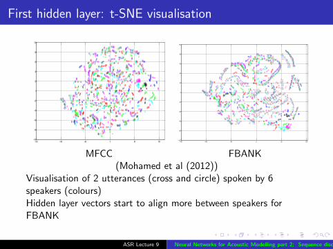
MFCC FBANK(Mohamed et al (2012))
Visualisation of 2 utterances (cross and circle) spoken by 6speakers (colours)MFCCs are more scattered than FBANKFBANK has more local structure than MFCCs
ASR Lecture 9 Neural Networks for Acoustic Modelling part 2; Sequence discriminative training10
First hidden layer: t-SNE visualisation
−150 −100 −50 0 50 100−100
−80
−60
−40
−20
0
20
40
60
80
100
Fig. 7. t-SNE 2-D map of the 1st layer of the fine-tuned hiddenactivity vectors using MFCC inputs.
−100 −80 −60 −40 −20 0 20 40 60 80 100−100
−50
0
50
100
150
Fig. 8. t-SNE 2-D map of the 8th layer of the fine-tuned hiddenactivity vectors using MFCC inputs.
formed using the discrete cosine transform, which encourages decor-related elements. We rank-order the dct features from lower-order(slow-moving) features to higher-order ones. For the generative pre-training phase, the dct features are disadvantaged because they arenot as strongly structured as the fbank features. To avoid a con-founding effect, we skipped pre-training and performed the compar-ison using only the fine-tuning from random initial weights. Table 2shows PER for fbank, dct, and MFCC inputs (11 input frames and1024 hidden units per layer) in 1, 2, and 3 hidden-layer neural net-works. dct features are worse than both fbank features and MFCCfeatures. This prompts us to ask why a lossless transformation causesthe input representation to perform worse (even when we skip a gen-erative pre-training step that favours more structured input), and howdct features can be worse than MFCC features, which are a subsetof them. We believe the answer is that higher-order dct features areuseless and distracting because all the important information is con-centrated in the first few features. In the fbank case the discriminantinformation is distributed across all coefficients. We conclude thatthe DBN has difficulty ignoring irrelevant input features. To test
this claim, we padded the MFCC vector with random noise to be ofthe same dimensionality as the dct features and then used them fornetwork training (MFCC+noise row in table 2). The MFCC perfor-mance was degraded by padding with noise. So it is not the higherdimensionality that matters but rather how the discriminant informa-tion is distributed over these dimensions.
Table 2. The PER deep nets using different features
Feature Dim 1lay 2lay 3layfbank 123 23.5% 22.6% 22.7%dct 123 26.0% 23.8% 24.6%
MFCC 39 24.3% 23.7% 23.8%MFCC+noise 123 26.3% 24.3% 25.1%
5. CONCLUSIONS
A DBN acoustic model has three main properties: It is a neuralnetwork, it has many layers of non-linear features, and it is pre-trained as a generative model. In this paper we investigated howeach of these three properties contributes to good phone recognitionon TIMIT. Additionally, we examined different types of input rep-resentation for DBNs by comparing recognition rates and also byvisualising the similarity structure of the input vectors and the hid-den activity vectors. We concluded that log filter-bank features arethe most suitable for DBNs because they better utilize the ability ofthe neural net to discover higher-order structure in the input data.
6. REFERENCES
[1] H. Bourlard and N. Morgan, Connectionist Speech Recognition:A Hybrid Approach, Kluwer Academic Publishers, 1993.
[2] H. Hermansky, D. Ellis, and S. Sharma, “Tandem connectionistfeature extraction for conventional HMM systems,” in ICASSP,2000, pp. 1635–1638.
[3] G. E. Hinton, S. Osindero, and Y. W. Teh, “A fast learning algo-rithm for deep belief nets,” Neural Computation, vol. 18, no. 7,pp. 1527–1554, 2006.
[4] A. Mohamed, G. Dahl, and G. Hinton, “Acoustic modeling us-ing deep belief networks,” IEEE Transactions on Audio, Speech,and Language Processing, 2011.
[5] G. Dahl, D. Yu, L. Deng, and A. Acero, “Context-dependentpre-trained deep neural networks for large vocabulary speechrecognition,” IEEE Transactions on Audio, Speech, and Lan-guage Processing, 2011.
[6] T. N. Sainath, B. Kingsbury, B. Ramabhadran, P. Fousek, P. No-vak, and A. Mohamed, “Making deep belief networks effectivefor large vocabulary continuous speech recognition,” in ASRU,2011.
[7] J.B. Allen, “How do humans process and recognize speech?,”IEEE Trans. Speech Audio Processing, vol. 2, no. 4, pp. 567–577, 1994.
[8] G. E. Hinton, “Training products of experts by minimizing con-trastive divergence,” Neural Computation, vol. 14, no. 8, pp.1711–1800, 2002.
[9] L.J.P. van der Maaten and G.E. Hinton, “Visualizing high-dimensional data using t-sne,” Journal of Machine LearningResearch, vol. 9, pp. 2579–2605, 2008.
are also close in the 2-D space. It starts by converting the pairwisedistances, dij in the high-dimensional space to joint probabilitiespij ∝ exp(−d2
ij). It then performs an iterative search for corre-sponding points in the 2-D space which give rise to a similar set ofjoint probabilities. To cope with the fact that there is much more vol-ume near to a high dimensional point than a low dimensional one,t-SNE computes the joint probability in the 2-D space by using aheavy tailed probability distribution qij ∝ (1 + d2
ij)−1. This leads
to 2-D maps that exhibit structure at many scales [9].For visualization only (they were not used for training or test-
ing), we used SA utterances from the TIMIT core test set speakers.These are the two utterances that were spoken by all 24 differentspeakers. Figures 3 and 4 show visualizations of fbank and MFCCfeatures for 6 speakers. Crosses refer to one utterance and circles re-fer to the other one, while different colours refer to different speak-ers. We removed the data points of the other 18 speakers to make themap less cluttered.
−100 −80 −60 −40 −20 0 20 40 60 80 100−150
−100
−50
0
50
100
150
Fig. 3. t-SNE 2-D map of fbank feature vectors
−100 −80 −60 −40 −20 0 20 40 60 80 100−100
−80
−60
−40
−20
0
20
40
60
80
100
Fig. 4. t-SNE 2-D map of MFCC feature vectorsMFCC vectors tend to be scattered all over the space as they have
decorrelated elements while fbank feature vectors have stronger sim-ilarities and are often aligned between different speakers for some
voiceless sounds (e.g. /s/, /sh/). This suggests that the fbank featurevectors are easier to model generatively as the data have strongerlocal structure than MFCC vectors. We can also see that DBNs aredoing some implicit normalization of feature vectors across differentspeakers when fbank features are used because they contain both thespoken content and style of the utterance which allows the DBN (be-cause of its distributed representations) to partially separate contentand style aspects of the input during the pre-training phase. Thismakes it easier for the discriminative fine-tuning phase to enhancethe propagation of content aspects to higher layers. Figures 5, 6, 7and 8 show the 1st and 8th layer features of fine-tuned DBNs trainedwith fbank and MFCC respectively. As we go higher in the network,hidden activity vectors from different speakers for the same segmentalign in both theMFCC and fbank cases but the alignment is strongerin the fbank case.
−150 −100 −50 0 50 100−100
−80
−60
−40
−20
0
20
40
60
80
100
Fig. 5. t-SNE 2-D map of the 1st layer of the fine-tuned hiddenactivity vectors using fbank inputs.
−100 −80 −60 −40 −20 0 20 40 60 80 100−100
−80
−60
−40
−20
0
20
40
60
80
100
Fig. 6. t-SNE 2-D map of the 8th layer of the fine-tuned hiddenactivity vectors using fbank inputs.
To refute the hypothesis that fbank features yield lower PERbecause of their higher dimensionality, we consider dct features,which are the same as fbank features except that they are trans-
MFCC FBANK(Mohamed et al (2012))
Visualisation of 2 utterances (cross and circle) spoken by 6speakers (colours)Hidden layer vectors start to align more between speakers forFBANK
ASR Lecture 9 Neural Networks for Acoustic Modelling part 2; Sequence discriminative training11

Eighth hidden layer: t-SNE visualisation
−150 −100 −50 0 50 100−100
−80
−60
−40
−20
0
20
40
60
80
100
Fig. 7. t-SNE 2-D map of the 1st layer of the fine-tuned hiddenactivity vectors using MFCC inputs.
−100 −80 −60 −40 −20 0 20 40 60 80 100−100
−50
0
50
100
150
Fig. 8. t-SNE 2-D map of the 8th layer of the fine-tuned hiddenactivity vectors using MFCC inputs.
formed using the discrete cosine transform, which encourages decor-related elements. We rank-order the dct features from lower-order(slow-moving) features to higher-order ones. For the generative pre-training phase, the dct features are disadvantaged because they arenot as strongly structured as the fbank features. To avoid a con-founding effect, we skipped pre-training and performed the compar-ison using only the fine-tuning from random initial weights. Table 2shows PER for fbank, dct, and MFCC inputs (11 input frames and1024 hidden units per layer) in 1, 2, and 3 hidden-layer neural net-works. dct features are worse than both fbank features and MFCCfeatures. This prompts us to ask why a lossless transformation causesthe input representation to perform worse (even when we skip a gen-erative pre-training step that favours more structured input), and howdct features can be worse than MFCC features, which are a subsetof them. We believe the answer is that higher-order dct features areuseless and distracting because all the important information is con-centrated in the first few features. In the fbank case the discriminantinformation is distributed across all coefficients. We conclude thatthe DBN has difficulty ignoring irrelevant input features. To test
this claim, we padded the MFCC vector with random noise to be ofthe same dimensionality as the dct features and then used them fornetwork training (MFCC+noise row in table 2). The MFCC perfor-mance was degraded by padding with noise. So it is not the higherdimensionality that matters but rather how the discriminant informa-tion is distributed over these dimensions.
Table 2. The PER deep nets using different features
Feature Dim 1lay 2lay 3layfbank 123 23.5% 22.6% 22.7%dct 123 26.0% 23.8% 24.6%
MFCC 39 24.3% 23.7% 23.8%MFCC+noise 123 26.3% 24.3% 25.1%
5. CONCLUSIONS
A DBN acoustic model has three main properties: It is a neuralnetwork, it has many layers of non-linear features, and it is pre-trained as a generative model. In this paper we investigated howeach of these three properties contributes to good phone recognitionon TIMIT. Additionally, we examined different types of input rep-resentation for DBNs by comparing recognition rates and also byvisualising the similarity structure of the input vectors and the hid-den activity vectors. We concluded that log filter-bank features arethe most suitable for DBNs because they better utilize the ability ofthe neural net to discover higher-order structure in the input data.
6. REFERENCES
[1] H. Bourlard and N. Morgan, Connectionist Speech Recognition:A Hybrid Approach, Kluwer Academic Publishers, 1993.
[2] H. Hermansky, D. Ellis, and S. Sharma, “Tandem connectionistfeature extraction for conventional HMM systems,” in ICASSP,2000, pp. 1635–1638.
[3] G. E. Hinton, S. Osindero, and Y. W. Teh, “A fast learning algo-rithm for deep belief nets,” Neural Computation, vol. 18, no. 7,pp. 1527–1554, 2006.
[4] A. Mohamed, G. Dahl, and G. Hinton, “Acoustic modeling us-ing deep belief networks,” IEEE Transactions on Audio, Speech,and Language Processing, 2011.
[5] G. Dahl, D. Yu, L. Deng, and A. Acero, “Context-dependentpre-trained deep neural networks for large vocabulary speechrecognition,” IEEE Transactions on Audio, Speech, and Lan-guage Processing, 2011.
[6] T. N. Sainath, B. Kingsbury, B. Ramabhadran, P. Fousek, P. No-vak, and A. Mohamed, “Making deep belief networks effectivefor large vocabulary continuous speech recognition,” in ASRU,2011.
[7] J.B. Allen, “How do humans process and recognize speech?,”IEEE Trans. Speech Audio Processing, vol. 2, no. 4, pp. 567–577, 1994.
[8] G. E. Hinton, “Training products of experts by minimizing con-trastive divergence,” Neural Computation, vol. 14, no. 8, pp.1711–1800, 2002.
[9] L.J.P. van der Maaten and G.E. Hinton, “Visualizing high-dimensional data using t-sne,” Journal of Machine LearningResearch, vol. 9, pp. 2579–2605, 2008.
are also close in the 2-D space. It starts by converting the pairwisedistances, dij in the high-dimensional space to joint probabilitiespij ∝ exp(−d2
ij). It then performs an iterative search for corre-sponding points in the 2-D space which give rise to a similar set ofjoint probabilities. To cope with the fact that there is much more vol-ume near to a high dimensional point than a low dimensional one,t-SNE computes the joint probability in the 2-D space by using aheavy tailed probability distribution qij ∝ (1 + d2
ij)−1. This leads
to 2-D maps that exhibit structure at many scales [9].For visualization only (they were not used for training or test-
ing), we used SA utterances from the TIMIT core test set speakers.These are the two utterances that were spoken by all 24 differentspeakers. Figures 3 and 4 show visualizations of fbank and MFCCfeatures for 6 speakers. Crosses refer to one utterance and circles re-fer to the other one, while different colours refer to different speak-ers. We removed the data points of the other 18 speakers to make themap less cluttered.
−100 −80 −60 −40 −20 0 20 40 60 80 100−150
−100
−50
0
50
100
150
Fig. 3. t-SNE 2-D map of fbank feature vectors
−100 −80 −60 −40 −20 0 20 40 60 80 100−100
−80
−60
−40
−20
0
20
40
60
80
100
Fig. 4. t-SNE 2-D map of MFCC feature vectorsMFCC vectors tend to be scattered all over the space as they have
decorrelated elements while fbank feature vectors have stronger sim-ilarities and are often aligned between different speakers for some
voiceless sounds (e.g. /s/, /sh/). This suggests that the fbank featurevectors are easier to model generatively as the data have strongerlocal structure than MFCC vectors. We can also see that DBNs aredoing some implicit normalization of feature vectors across differentspeakers when fbank features are used because they contain both thespoken content and style of the utterance which allows the DBN (be-cause of its distributed representations) to partially separate contentand style aspects of the input during the pre-training phase. Thismakes it easier for the discriminative fine-tuning phase to enhancethe propagation of content aspects to higher layers. Figures 5, 6, 7and 8 show the 1st and 8th layer features of fine-tuned DBNs trainedwith fbank and MFCC respectively. As we go higher in the network,hidden activity vectors from different speakers for the same segmentalign in both theMFCC and fbank cases but the alignment is strongerin the fbank case.
−150 −100 −50 0 50 100−100
−80
−60
−40
−20
0
20
40
60
80
100
Fig. 5. t-SNE 2-D map of the 1st layer of the fine-tuned hiddenactivity vectors using fbank inputs.
−100 −80 −60 −40 −20 0 20 40 60 80 100−100
−80
−60
−40
−20
0
20
40
60
80
100
Fig. 6. t-SNE 2-D map of the 8th layer of the fine-tuned hiddenactivity vectors using fbank inputs.
To refute the hypothesis that fbank features yield lower PERbecause of their higher dimensionality, we consider dct features,which are the same as fbank features except that they are trans-
MFCC FBANK(Mohamed et al (2012))
Visualisation of 2 utterances (cross and circle) spoken by 6speakers (colours)In the final hidden layer, the hidden layer outputs for the samephone are well-aligned across speakers for both MFCC and FBANK– but stronger for FBANK
ASR Lecture 9 Neural Networks for Acoustic Modelling part 2; Sequence discriminative training12

Visualising neural networks
How to visualise NN layers? “t-SNE” (stochastic neighbourembedding using t-distribution) projects high dimensionvectors (e.g. the values of all the units in a layer) into 2dimensions
t-SNE projection aims to keep points that are close in highdimensions close in 2 dimensions by comparing distributionsover pairwise distances between the high dimensional and 2dimensional spaces – the optimisation is over the positions ofpoints in the 2-d space
Are the differences due to FBANK being higher dimension(41× 3 = 123) than MFCC (13× 3 = 39)?
No – Using higher dimension MFCCs, or just adding noisydimmensions to MFCCs results in higher error rate
Why? – In FBANK the useful information is distributed overall the features; in MFCC it is concentrated in the first few.
ASR Lecture 9 Neural Networks for Acoustic Modelling part 2; Sequence discriminative training13
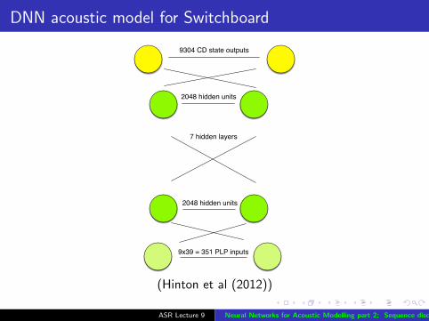
DNN acoustic model for Switchboard
7 hidden layers
2048 hidden units
9304 CD state outputs
2048 hidden units
9x39 = 351 PLP inputs
(Hinton et al (2012))
ASR Lecture 9 Neural Networks for Acoustic Modelling part 2; Sequence discriminative training14

Example: hybrid HMM/DNN large vocabularyconversational speech recognition (Switchboard)
Recognition of American English conversational telephonespeech (Switchboard)
Baseline context-dependent HMM/GMM system
9,304 tied statesDiscriminatively trained (BMMI — similar to MPE)39-dimension PLP (+ derivatives) featuresTrained on 309 hours of speech
Hybrid HMM/DNN system
Context-dependent — 9304 output units obtained from Viterbialignment of HMM/GMM system7 hidden layers, 2048 units per layer
DNN-based system results in significant word error ratereduction compared with GMM-based system
Pretraining not necessary on larger tasks (empirical result)
ASR Lecture 9 Neural Networks for Acoustic Modelling part 2; Sequence discriminative training15

DNN vs GMM on large vocabulary tasks (Experimentsfrom 2012)
IEEE SIGNAL PROCESSING MAGAZINE [92] NOVEMBER 2012
and model-space discriminative training is applied using the BMMI or MPE criterion.
Using alignments from a baseline system, [32] trained a DBN-DNN acoustic model on 50 h of data from the 1996 and 1997 English Broadcast News Speech Corpora [37]. The DBN-DNN was trained with the best-performing LVCSR features, specifically the SAT+DT features. The DBN-DNN architecture con-sisted of six hidden layers with 1,024 units per layer and a final softmax layer of 2,220 context-dependent states. The SAT+DT feature input into the first layer used a context of nine frames. Pretraining was performed fol-lowing a recipe similar to [42].
Two phases of fine-tuning were performed. During the first phase, the cross entropy loss was used. For cross entropy train-ing, after each iteration through the whole training set, loss is measured on a held-out set and the learning rate is annealed (i.e., reduced) by a factor of two if the held-out loss has grown or improves by less than a threshold of 0.01% from the previ-ous iteration. Once the learning rate has been annealed five times, the first phase of fine-tuning stops. After weights are learned via cross entropy, these weights are used as a starting point for a second phase of fine-tuning using a sequence crite-rion [37] that utilizes the MPE objective function, a discrimi-native objective function similar to MMI [7] but which takes into account phoneme error rate.
A strong SAT+DT GMM-HMM baseline system, which con-sisted of 2,220 context-dependent states and 50,000 Gaussians, gave a WER of 18.8% on the EARS Dev-04f set, whereas the DNN-HMM system gave 17.5% [50].
SUMMARY OF THE MAIN RESULTS FOR DBN-DNN ACOUSTIC MODELS ON LVCSR TASKSTable 3 summarizes the acoustic modeling results described above. It shows that DNN-HMMs consistently outperform GMM-HMMs that are trained on the same amount of data, sometimes by a large margin. For some tasks, DNN-HMMs also outperform GMM-HMMs that are trained on much more data.
SPEEDING UP DNNs AT RECOGNITION TIMEState pruning or Gaussian selection methods can be used to make GMM-HMM systems computationally efficient at recogni-tion time. A DNN, however, uses virtually all its parameters at every frame to compute state likelihoods, making it potentially
much slower than a GMM with a comparable number of parame-ters. Fortunately, the time that a DNN-HMM system requires to recognize 1 s of speech can be reduced from 1.6 s to 210 ms, without decreasing recognition accuracy, by quantizing the weights down to 8 b and using the very fast SIMD primitives for fixed-point computation that are provided by a modern x86 cen-
tral processing unit [49]. Alternatively, it can be reduced to 66 ms by using a graphics processing unit (GPU).
ALTERNATIVE PRETRAINING METHODS FOR DNNsPretraining DNNs as generative models led to better recognition results on TIMIT and subsequently on a variety of LVCSR tasks. Once it was shown that DBN-DNNs could learn good acoustic models, further research revealed that they could be trained in many different ways. It is possible to learn a DNN by starting with a shallow neural net with a single hidden layer. Once this net has been trained discriminatively, a second hidden layer is interposed between the first hidden layer and the softmax output units and the whole network is again discriminatively trained. This can be continued until the desired number of hidden layers is reached, after which full backpropagation fine-tuning is applied.
This type of discriminative pretraining works well in prac-tice, approaching the accuracy achieved by generative DBN pre-training and further improvement can be achieved by stopping the discriminative pretraining after a single epoch instead of multiple epochs as reported in [45]. Discriminative pretraining has also been found effective for the architectures called “deep convex network” [51] and “deep stacking network” [52], where pretraining is accomplished by convex optimization involving no generative models.
Purely discriminative training of the whole DNN from ran-dom initial weights works much better than had been thought,
provided the scales of the initial weights are set carefully, a large amount of labeled training data is available, and minibatch sizes over training epochs are set appropri-ately [45], [53]. Nevertheless, gen-erative pretraining still improves test performance, sometimes by a significant amount.
Layer-by-layer generative pre-training was originally done using RBMs, but various types of
[TABLE 3] A COMPARISON OF THE PERCENTAGE WERs USING DNN-HMMs AND GMM-HMMs ON FIVE DIFFERENT LARGE VOCABULARY TASKS.
TASK HOURS OF TRAINING DATA DNN-HMM
GMM-HMM WITH SAME DATA
GMM-HMM WITH MORE DATA
SWITCHBOARD (TEST SET 1) 309 18.5 27.4 18.6 (2,000 H)
SWITCHBOARD (TEST SET 2) 309 16.1 23.6 17.1 (2,000 H)
ENGLISH BROADCAST NEWS 50 17.5 18.8
BING VOICE SEARCH (SENTENCE ERROR RATES) 24 30.4 36.2
GOOGLE VOICE INPUT 5,870 12.3 16.0 (22 5,870 H)
YOUTUBE 1,400 47.6 52.3
DISCRIMINATIVE PRETRAININGHAS ALSO BEEN FOUND EFFECTIVE FOR THE ARCHITECTURES CALLED “DEEP CONVEX NETWORK” AND
“DEEP STACKING NETWORK,” WHERE PRETRAINING IS ACCOMPLISHED BY CONVEX OPTIMIZATION INVOLVING
NO GENERATIVE MODELS.
(Hinton et al (2012))
ASR Lecture 9 Neural Networks for Acoustic Modelling part 2; Sequence discriminative training16
Sequence Discriminative Training
ASR Lecture 9 Neural Networks for Acoustic Modelling part 2; Sequence discriminative training17
Training HMM/GMM acoustic models
Use forward-backward algorithm to estimate the stateoccupation probabilities (E-step), which are used tore-estimate the parameters (M-step)
Maximum likelihood estimation: estimate the parameters sothat the model reproduces the training data with the greatestprobability (maximum likelihood)
Discriminative training: directly estimate the parameters so asto make the fewest classification errors (optimize the worderror rate)
Focus on learning boundaries between classesConsider incorrect word sequences as well as correct wordsequencesThis is related to direct optimisation of the posteriorprobability of the words given the acoustics P(W | X)
ASR Lecture 9 Neural Networks for Acoustic Modelling part 2; Sequence discriminative training18

Hybrid HMM/NN acoustic models
Neural networks are discriminatively trained at the frame level
Consider a context-dependent DNN
Output is a softmax over HMM statesTraining involves increasing the probability of the correct state– and hence decreasing the probabilities of the others, sinceprobabilities sum to 1Frame-level discrimination – the network learns to optimisediscrimination at the frame level by choosing the best state ateach time frame
Sequence discrimination – train the system to select thebest sequence of frames by increasing the probability of thebest sequence and decreasing the probability of all competingsequences
Can train both GMM and DNN based models using sequencediscrimination
ASR Lecture 9 Neural Networks for Acoustic Modelling part 2; Sequence discriminative training19
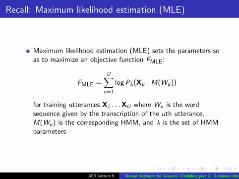
Recall: Maximum likelihood estimation (MLE)
Maximum likelihood estimation (MLE) sets the parameters soas to maximize an objective function FMLE:
FMLE =U∑
u=1
logPλ(Xu | M(Wu))
for training utterances X1 . . .XU where Wu is the wordsequence given by the transcription of the uth utterance,M(Wu) is the corresponding HMM, and λ is the set of HMMparameters
ASR Lecture 9 Neural Networks for Acoustic Modelling part 2; Sequence discriminative training20

Maximum mutual information estimation
Maximum mutual information estimation (MMIE) aims todirectly maximise the posterior probability (sometimes calledconditional maximum likelihood). Using the same notation asbefore, with P(w) representing the language model probabilityof word sequence w :
FMMIE =U∑
u=1
logPλ(M(Wu) | Xu)
=U∑
u=1
logPλ(Xu | M(Wu))P(Wu)∑w ′ Pλ(Xu | M(w ′))P(w ′)
ASR Lecture 9 Neural Networks for Acoustic Modelling part 2; Sequence discriminative training21

Maximum mutual information estimation
Maximum mutual information estimation (MMIE) aims todirectly maximise the posterior probability (sometimes calledconditional maximum likelihood). Using the same notation asbefore, with P(w) representing the language model probabilityof word sequence w :
FMMIE =U∑
u=1
logPλ(M(Wu) | Xu)
FMLE =U∑
u=1
logPλ(Xu | M(Wu))P(Wu)∑w ′ Pλ(Xu | M(w ′))P(w ′)
ASR Lecture 9 Neural Networks for Acoustic Modelling part 2; Sequence discriminative training21

Maximum mutual information estimation
FMMIE =U∑
u=1
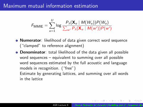
logPλ(Xu | M(Wu))P(Wu)∑w ′ Pλ(Xu | M(w ′))P(w ′)
Numerator: likelihood of data given correct word sequence(“clamped” to reference alignment)
Denominator: total likelihood of the data given all possibleword sequences – equivalent to summing over all possibleword sequences estimated by the full acoustic and languagemodels in recognition. (“free”)Estimate by generating lattices, and summing over all wordsin the lattice
The objective function FMMIE is optimised by making thecorrect word sequence likely (maximise the numerator), andall other word sequences unlikely (minimise the denominator)
ASR Lecture 9 Neural Networks for Acoustic Modelling part 2; Sequence discriminative training22

Maximum mutual information estimation
FMMIE =U∑
u=1
logPλ(Xu | M(Wu))P(Wu)∑w ′ Pλ(Xu | M(w ′))P(w ′)
Numerator: likelihood of data given correct word sequence(“clamped” to reference alignment)
Denominator: total likelihood of the data given all possibleword sequences – equivalent to summing over all possibleword sequences estimated by the full acoustic and languagemodels in recognition. (“free”)Estimate by generating lattices, and summing over all wordsin the lattice
The objective function FMMIE is optimised by making thecorrect word sequence likely (maximise the numerator), andall other word sequences unlikely (minimise the denominator)
ASR Lecture 9 Neural Networks for Acoustic Modelling part 2; Sequence discriminative training22

MPE: Minimum phone error
Basic idea adjust the optimization criterion so it is directlyrelated to word error rate
Minimum phone error (MPE) criterion
A(W ,Wu) is the phone transcription accuracy of the sentenceW given the reference Wu
FMPE is a weighted average over all possible sentences w ofthe raw phone accuracy
Although MPE optimizes a phone accuracy level, it does so inthe context of a word-level system: it is optimized by findingprobable sentences with low phone error rates
ASR Lecture 9 Neural Networks for Acoustic Modelling part 2; Sequence discriminative training23

MPE: Minimum phone error
Basic idea adjust the optimization criterion so it is directlyrelated to word error rate
Minimum phone error (MPE) criterion
FMPE =U∑
u=1
log
∑W Pλ(Xu | M(W ))P(W )A(W ,Wu)∑
W ′ Pλ(Xu | M(W ′))P(W ′)
A(W ,Wu) is the phone transcription accuracy of the sentenceW given the reference Wu
FMPE is a weighted average over all possible sentences w ofthe raw phone accuracy
Although MPE optimizes a phone accuracy level, it does so inthe context of a word-level system: it is optimized by findingprobable sentences with low phone error rates
ASR Lecture 9 Neural Networks for Acoustic Modelling part 2; Sequence discriminative training23

MPE: Minimum phone error
Basic idea adjust the optimization criterion so it is directlyrelated to word error rate
Minimum phone error (MPE) criterion
FMMIE =U∑
u=1
log
∑WPλ(Xu | M(Wu))P(Wu)A(W ,Wu)∑
W ′ Pλ(Xu | M(W ′))P(W ′)
A(W ,Wu) is the phone transcription accuracy of the sentenceW given the reference Wu
FMPE is a weighted average over all possible sentences w ofthe raw phone accuracy
Although MPE optimizes a phone accuracy level, it does so inthe context of a word-level system: it is optimized by findingprobable sentences with low phone error rates
ASR Lecture 9 Neural Networks for Acoustic Modelling part 2; Sequence discriminative training23

MPE: Minimum phone error
Basic idea adjust the optimization criterion so it is directlyrelated to word error rate
Minimum phone error (MPE) criterion
FMPE =U∑
u=1
log
∑W Pλ(Xu | M(W ))P(W )A(W ,Wu)∑
W ′ Pλ(Xu | M(W ′))P(W ′)
A(W ,Wu) is the phone transcription accuracy of the sentenceW given the reference Wu
FMPE is a weighted average over all possible sentences w ofthe raw phone accuracy
Although MPE optimizes a phone accuracy level, it does so inthe context of a word-level system: it is optimized by findingprobable sentences with low phone error rates
ASR Lecture 9 Neural Networks for Acoustic Modelling part 2; Sequence discriminative training23

Sequence training of hybrid HMM/DNN systems
It is possible to train HMM/NN systems using a MMI-typeobjective function
Forward- and back-propagation equations are structurallysimilar to forward and backward recursions in HMM training
Initially train DNN framewise using cross-entropy (CE) errorfunction
Use CE-trained model to generate alignments and lattices forsequence trainingUse CE-trained weights to initialise weights for sequencetraining
Train using back-propagation with sequence training objectivefunction (e.g. MMI)
ASR Lecture 9 Neural Networks for Acoustic Modelling part 2; Sequence discriminative training24

Sequence training results on Switchboard (Kaldi)
Results on Switchboard “Hub 5 ’00” test set, trained on 300h trainingset, comparing maximum likelihood (ML) and discriminative (BMMI)trained GMMs with framewise cross-entropy (CE) and sequence trained(MMI) DNNs. GMM systems use speaker adaptive training (SAT).All systems had 8859 tied triphone states.GMMs – 200k GaussiansDNNs – 6 hidden layers each with 2048 hidden units
SWB CHE Total
GMM ML (+SAT) 21.2 36.4 28.8GMM BMMI (+SAT) 18.6 33.0 25.8
DNN CE 14.2 25.7 20.0DNN MMI 12.9 24.6 18.8
Veseley et al, 2013.
ASR Lecture 9 Neural Networks for Acoustic Modelling part 2; Sequence discriminative training25

Summary
DNN/HMM systems (hybrid systems) give a significantimprovement over GMM/HMM systems
Compared with 1990s NN/HMM systems, DNN/HMMsystems
model context-dependent tied states with a much wider outputlayerare deeper – more hidden layerscan use correlated features (e.g. FBANK)
Sequence training: discriminatively optimise GMM or DNN toa sentence (sequence) level criterion rather than a frame levelcriterion
Next lecture: Speaker adaptation
ASR Lecture 9 Neural Networks for Acoustic Modelling part 2; Sequence discriminative training26

Reading
G Hinton et al (Nov 2012). “Deep neural networks for acousticmodeling in speech recognition”, IEEE Signal Processing Magazine,29(6), 82–97.http://ieeexplore.ieee.org/document/6296526
A Mohamed et al (2012). “Unserstanding how deep belief networksperform acoustic modelling”, Proc ICASSP-2012. http:
//www.cs.toronto.edu/~asamir/papers/icassp12_dbn.pdf
HMM discriminative training: Sec 27.3.1 of: S Young (2008),“HMMs and Related Speech Recognition Technologies”, in SpringerHandbook of Speech Processing, Benesty, Sondhi and Huang (eds),chapter 27, 539–557. http://www.inf.ed.ac.uk/teaching/
courses/asr/2010-11/restrict/Young.pdf
NN sequence training: K Vesely et al (2013),“Sequence-discriminative training of deep neural networks”,Interspeech-2013, http://homepages.inf.ed.ac.uk/aghoshal/pubs/is13-dnn_seq.pdf
ASR Lecture 9 Neural Networks for Acoustic Modelling part 2; Sequence discriminative training27