Neural Network Control and Wireless Sensor Network-based

14

Neural Network Control and Wireless Sensor Network-based Localization of Quadrotor UAV

Formations

Travis Dierks and S. Jagannathan Missouri University of Science and Technology

United States of America

1. Introduction

In recent years, quadrotor helicopters have become a popular unmanned aerial vehicle (UAV) platform, and their control has been undertaken by many researchers (Dierks & Jagannathan, 2008). However, a team of UAV’s working together is often more effective than a single UAV in scenarios like surveillance, search and rescue, and perimeter security. Therefore, the formation control of UAV’s has been proposed in the literature. Saffarian and Fahimi present a modified leader-follower framework and propose a model predictive nonlinear control algorithm to achieve the formation (Saffarian & Fahimi, 2008). Although the approach is verified via numerical simulations, proof of convergence and stability is not provided. In the work of Fierro et al., cylindrical coordinates and contributions from wheeled mobile robot formation control (Desai et al., 1998) are considered in the development of a leader-follower based formation control scheme for aircrafts whereas the complete dynamics are assumed to be known (Fierro et al., 2001). The work by Gu et al. proposes a solution to the leader-follower formation control problem involving a linear inner loop and nonlinear outer-loop control structure, and experimental results are provided (Gu et al., 2006). The associated drawbacks are the need for a dynamic model and the measured position and velocity of the leader has to be communicated to its followers. Xie et al. present two nonlinear robust formation controllers for UAV’s where the UAV’s are assumed to be flying at a constant altitude. The first approach assumes that the velocities and accelerations of the leader UAV are known while the second approach relaxes this assumption (Xie et al., 2005). In both the designs, the dynamics of the UAV’s are assumed to be available. Then, Galzi and Shtessel propose a robust formation controller based on higher order sliding mode controllers in the presence of bounded disturbances (Galzi & Shtessel, 2006). In this work, we propose a new leader-follower formation control framework for quadrotor UAV’s based on spherical coordinates where the desired position of a follower UAV is

specified using a desired separation, ds , and a desired- angle of incidence,

dα and bearing,

dβ . Then, a new control law for leader-follower formation control is derived using neural

networks (NN) to learn the complete dynamics of the UAV online, including unmodeled dynamics like aerodynamic friction in the presence of bounded disturbances. Although a

www.intechopen.com

Aerial Vehicles

288

quadrotor UAV is underactuated, a novel NN virtual control input scheme for leader follower formation control is proposed which allows all six degrees of freedom of the UAV to be controlled using only four control inputs. Finally, we extend a graph theory-based scheme for discovery, localization and cooperative control. Discovery allows the UAV’s to form into an ad hoc mobile sensor network whereas localization allows each UAV to estimate its position and orientation relative to its neighbors and hence the formation shape. This chapter is organized as follows. First, in Section 2, the leader-follower formation control problem for UAV’s is introduced, and required background information is presented. Then, the NN control law is developed for the follower UAV’s as well as the formation leader, and the stability of the overall formation is presented in Section 3. In Section 4, the localization and routing scheme is introduced for UAV formation control while Section 5 presents numerical simulations, and Section 6 provides some concluding remarks.

2. Background

2.1 Quadrotor UAV Dynamics

Consider a quadrotor UAV with six DOF defined in the inertial coordinate frame , aE , as aT Ezyx ∈],,,,,[ ψθφ where aT Ezyx ∈= ],,[ρ are the position coordinates of the UAV

and aT E∈=Θ ],,[ ψθφ describe its orientation referred to as roll, pitch, and yaw,

respectively. The translational and angular velocities are expressed in the body fixed frame

attached to the center of mass of the UAV, bE , and the dynamics of the UAV in the body fixed frame can be written as (Dierks & Jagannathan, 2008)

d

x

URG

N

vNvS

vM τ

ωωω

ω++⎥⎦

⎤⎢⎣⎡

+⎥⎦⎤⎢⎣

⎡+⎥⎦⎤⎢⎣

⎡=⎥⎦

⎤⎢⎣⎡

132

1

0

)(

)(

)()(

$$ (1)

where [ ] 6

2100 ℜ∈=TTuuU ,

66

33

3366

33

3333

)(0

0)()(,

0

0x

x

xx

x

xx

JS

mSS

J

mIM ℜ∈⎥⎦

⎤⎢⎣⎡−

=ℜ∈⎥⎦⎤⎢⎣

⎡=

ω

ωω

and m is a positive scalar that represents the total mass of the UAV, 33xJ ℜ∈ represents the

positive definite inertia matrix, 3],,[)( ℜ∈= T

zbybxb vvvtv represents the translational

velocity, [ ] 3,,)( ℜ∈=T

zbybxbt ωωωω represents the angular velocity, 2,1,)( 13 =ℜ∈• iN x

i,

are the nonlinear aerodynamic effects, 1

1 ℜ∈u provides the thrust along the z-direction,

3

2 ℜ∈u provides the rotational torques, 6

21 ],[ ℜ∈= TT

d

T

dd τττ and 2,1,3 =ℜ∈ idiτ

represents unknown, but bounded disturbances such thatMd ττ < for all time t ,

withMτ being a known positive constant, nxn

nxnI ℜ∈ is an nxn identity matrix, and

mxl

mxl ℜ∈0 represents an mxl matrix of all zeros. Furthermore, 3)( ℜ∈RG represents the

www.intechopen.com

Neural Network Control and Wireless Sensor Network-based Localization of Quadrotor UAV Formations

289

gravity vector defined asz

T EmgRRG )()( Θ= where T

zE ]1,0,0[= is a unit vector in the

inertial coordinate frame, 2/81.9 smg = , and 33)( xS ℜ∈• is the general form of a skew

symmetric matrix defined as in (Dierks & Jagannathan, 2008). It is important to highlight

0)( =wSwT γ for any vector 3ℜ∈w , and this property is commonly referred to as the skew

symmetric property (Lewis et al., 1999). The matrix 33)( xR ℜ∈Θ is the translational rotation matrix which is used to relate a vector in

the body fixed frame to the inertial coordinate frame defined as (Dierks & Jagannathan, 2008)

⎥⎥⎥⎦

⎤⎢⎢⎢⎣

⎡−

−+

+−

==Θ

θφθφθ

ψφψθφψφψθφψθ

ψφψθφψφψθφψθ

cccss

cssscccssssc

sscscsccsscc

RR )( (2)

where the abbreviations)(•s and

)(•c have been used for )sin(• and )cos(• , respectively. It

is important to note thatTRR =−1

, )(ωRSR =$ and TT RSR )(ω−=$ . It is also necessary

to define a rotational transformation matrix from the fixed body to the inertial coordinate frame as (Dierks & Jagannathan, 2008)

⎥⎥⎥⎦

⎤⎢⎢⎢⎣

⎡−==Θ

θφθφ

φφ

θφθφ

cccs

sc

tcts

TT

0

0

1

)( (3)

where the abbreviation)(•t has been used for )tan(• . The transformation matrices R and T

are nonsingular as long as ( ) ( ),22 πφπ <<− ( ) ( )22 πθπ <<− and πψπ ≤≤− . These

regions will be assumed throughout the development of this work, and will be referred to as the stable operation regions of the UAV. Under these flight conditions, it is observed that

maxRRF

= andmaxTT

F< for known constants

maxR andmaxT (Neff et al., 2007).

Finally, the kinematics of the UAV can be written as

ω

ρ

T

Rv

=Θ

=

$$

(4)

2.2 Neural Networks

In this work, two-layer NN’s are considered consisting of one layer of randomly assigned

constant weights axL

NV ℜ∈ in the first layer and one layer of tunable weights Lxb

NW ℜ∈ in

the second with a inputs,b outputs, and L hidden neurons. A compromise is made here

between tuning the number of layered weights with computational complexity. The universal approximation property for NN's (Lewis et al., 1999) states that for any smooth

function )( NN xf , there exists a NN such that NN

T

N

T

NNN xVWxf εσ += )()( whereNε is the

bounded NN functional approximation error such thatMN εε < ,for a known constant

Mε

www.intechopen.com

Aerial Vehicles

290

and La ℜ→ℜ⋅ :)(σ is the activation function in the hidden layers. It has been shown that

by randomly selecting the input layer weightsNV , the activation function )()( N

T

NN xVx σσ =

forms a stochastic basis, and thus the approximation property holds for all inputs, a

Nx ℜ∈ ,

in the compact set S . The sigmoid activation function is considered here. Furthermore, on

any compact subset ofnℜ , the target NN weights are bounded by a known positive value,

MW , such that MFN WW ≤ . For complete details of the NN and its properties, see (Lewis et

al., 1999).

2.3 Three Dimensional Leader-Follower Formation Control

Throughout the development, the follower UAV’s will be denoted with a subscript ‘j’ while the formation leader will be denoted by the subscript ‘i’. To begin the development, an alternate reference frame is defined by rotating the inertial coordinate frame about the z-axis

by the yaw angle of follower j, jψ , and denoted by a

jE . In order to relate a vector in

aE toa

jE , the transformation matrix is given by

⎥⎥⎥⎦

⎤⎢⎢⎢⎣

⎡−=

100

0cossin

0sincos

jj

jj

ajR ψψ

ψψ, (5)

where1−= aj

T

aj RR .

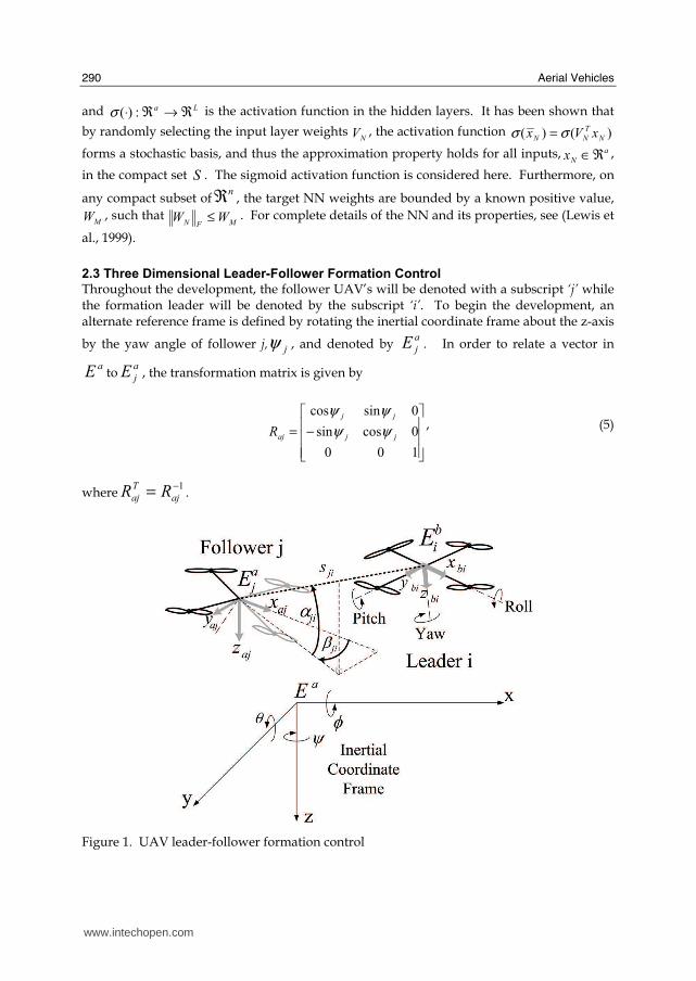
Figure 1. UAV leader-follower formation control

www.intechopen.com


291

The objective of the proposed leader-follower formation control approach is for the follower

UAV to maintain a desired separation, jids , at a desired angle of incidence, a

jjid E∈α ,

and bearing, a

jjid E∈β , with respect to its leader. The incidence angle is measured from

the ajaj yx − plane of follower j while the bearing angle is measured from the positive ajx -

axis as shown in Figure 1. It is important to observe that each quantity is defined relative to the follower j instead of the leader i (Fierro et al., 2001), (Desai et al., 1998). Additionally, in order to specify a unique configuration of follower j with respect to its leader, the desired

yaw of follower j is selected to be the yaw angle of leader i, a

i E∈ψ as in (Saffarian &

Fahimi, 2008). Using this approach, the measured separation between follower j and leader

i is written as

jiji

T

ajji sR Ξ=− ρρ , (6)

where

⎥⎥⎥⎦

⎤⎢⎢⎢⎣

⎡=Ξ

ji

jiji

jiji

ji

α

βα

βα

sin

sincos

coscos. (7)

Thus, to solve the leader-follower formation control problem in the proposed framework, a control velocity must be derived to ensure

⎪⎭⎪⎬⎫

=−=−

=−=−

∞→∞→

∞→∞→

0)(lim,0)(lim

,0)(lim,0)(lim

jjdt

jijidt

jijidt

jijidt

ss

ψψαα

ββ. (8)

Throughout the development,jids ,

jidα andjidβ will be taken as constants, while the constant

total mass,jm , is assumed to be known. Additionally, it will be assumed that reliable

communication between the leader and its followers is available, and the leader

communicates its measured orientation,iΘ , and its desired states,

ididid ψψψ $$$ ,, , idid vv $, . This

is a far less stringent assumption than assuming the leader communicates all of its measured states to its followers (Gu et al., 2006). Additionally, future work will relax this assumption. In the following section, contributions from single UAV control will be considered and extended to the leader-follower formation control of UAV’s.

3. Leader-Follower Formation Tracking Control

In single UAV control literature, the overall control objective UAV j is often to track a

desired trajectory, T

jdjdjdjd zyx ],,[=ρ , and a desired yaw jdψ while maintaining a

stable flight configuration (Dierks & Jagannathan, 2008). The velocity jzbv is directly

www.intechopen.com

Aerial Vehicles

292

controllable with the thrust input. However, in order to control the translational velocities

jxbv and jybv , the pitch and roll must be controlled, respectively, thus redirecting the

thrust. With these objectives in mind, the frameworks for single UAV control are extended to UAV formation control as follows.

3.1 Follower UAV Control Law

Given a leader i subject to the dynamics and kinematics (1) and (4), respectively, define a reference trajectory at a desired separation

jids , at a desired angle of incidence, jidα , and

bearing, jidβ for follower j given by

jidjid

T

ajdijd sR Ξ−= ρρ (9)

whereajdR is defined as in (5) and written in terms of

jdψ , and jidΞ is written in terms of the

desired angle of incidence and bearing, jidjid βα , ,respectively, similarly to (7). Next, using

(6) and (9), define the position tracking error as

a

jidjid

T

ajdjiji

T

ajjjdj EsRsRe ∈Ξ−Ξ=−= ρρρ (10)

which can be measured using local sensor information. To form the position tracking error

dynamics, it is convenient to rewrite (10) asjidjid

T

ajdjij sRe Ξ−−= ρρρrevealing

jidjid

T

ajdjjiij sRvRvRe Ξ−−= $$ ρ. (11)

Next, select the desired translational velocity of follower j to stabilize (11)

( ) b

jjjidjid

T

ajdidi

T

j

T

jdzjdyjdxjd EeKsRvRRvvvv ∈+Ξ−== ρρ$][ (12)

where 33},,{ x

zjyjxjj kkkdiagK ℜ∈= ρρρρis a diagonal positive definite design matrix of

positive design constants and idv is the desired translational velocity of leader i. Next, the

translational velocity tracking error system is defined as

.jjd

jzb

jyb

jxb

jdz

jdy

jdx

jvz

jvy

jvx

jv vv

v

v

v

v

v

v

e

e

e

e −=

⎥⎥⎥⎦

⎤⎢⎢⎢⎣

⎡−

⎥⎥⎥⎦

⎤⎢⎢⎢⎣

⎡=

⎥⎥⎥⎦

⎤⎢⎢⎢⎣

⎡=

. (13)

Applying (12) to (11) while observingjvjdj evv −= and similarly

iidiv vve −= , reveals the

closed loop position error dynamics to be rewritten as

ivijvjjjj eReReKe −+−= ρρρ$ . (14)

www.intechopen.com


293

Next, the translational velocity tracking error dynamics are developed. Differentiating (13), observing

( ) ( )jidjid

T

ajdjjiij

T

jjidjid

T

ajdidiidii

T

jjdjjd sRvRvRKRsRvRvSRRvSv Ξ−−+Ξ−++−= $$$$$ ρωω )()( ,

substituting the translational velocity dynamics in (1), and adding and subtracting

))(( jdjidij

T

j vRvRKR +ρ reveals

( )( ) )()(

)()()( 111

jvjivij

T

jjjjvjjjidjidajdidiidii

T

j

jdjjzjjjjvjjjjjjdjv

eReRKReKeRKsRvRvSRR

mEumRGeSmvNvve

−−−+Ξ−++

−−−−−=−=

ρρρρω

τω

$$$

$$$. (15)

Next, we rewrite (2) in terms of the scaled desired orientation

vector, T

jdjdjdjd ][ ψφθ=Θ where )2( maxdjdjd θπθθ = , )2( maxdjdjd φπφφ = , and )2,0(max πθ ∈d

and )2,0(max πφ ∈d are the maximum desired roll and pitch, respectively, define )( jdjjd RR Θ= ,

and add and subtract jjd mRG /)( and

j

T

jdR Λ withρρρ jjjvjjjidjid

T

ajdidij eKeRKsRvR −+Ξ−=Λ $$$ to jve$

to yield

11111 )()( jdivijjjzjcjcjjcj

T

jdjjdjv eRKmEuxfARmRGe τρ −−−+Λ+−=$ (16)

where 33

1 }1),cos(),{cos( x

jdjdjc diagA ℜ∈= φθ and

( )( )ρρρρ ωω jjj

T

jidii

T

jjjjjvjjvjjjc

j

T

jd

T

jjjjjdjccjcj

eKKRvSRRmvNeSeRKA

RRmRGmRGAxf

)1()()()(

)()()()(

1

1

1

1

111

−++−−

+Λ−+−=

−

−

(17)

is an unknown function which can be rewritten as [ ] 3

13121111 )( ℜ∈=T

jcjcjcjcjc fffxf . In the

forthcoming development, the approximation properties of NN will be utilized to estimate

the unknown function )( 11 jcjc xf by bounded ideal weights T

jc

T

jc VW 11, such that

11 McF

jc WW ≤ for an unknown constant 1McW , and written as

111111 )()( jcjc

T

jc

T

jcjcjc xVWxf εσ +=

where 11 Mcjc εε ≤ is the bounded NN approximation error where

1Mcε is a known constant.

The NN estimate of 1jcf is written as ( ) 111111ˆˆˆˆˆjc

T

jcjc

T

jc

T

jcjc WxVWf σσ ==

T

jc

T

jcjc

T

jcjc

T

jc WWW ]ˆˆˆˆˆˆ[ 113112111 σσσ= where T

jcW 1ˆ is the NN estimate of T

jcW 1, 3,2,1,ˆ

1 =iW T

ijcis the

thi row of T

jcW 1ˆ , and

1ˆjcx is the NN input defined as

TT

j

T

jv

T

j

T

jjdjdjd

T

id

T

id

T

jd

T

j

T

i

T

jjc eevvvvx ]1[ˆ1 ρωψψψ $$$$ΛΘΘ= .

Note that 1

ˆjcx is an estimate of

1jcx since the follower does not knowiω . However,

iΘ is

directly related toiω ; therefore, it is included instead.

Remark 1: In the development of (16), the scaled desired orientation vector was utilized as a design tool to specify the desired pitch and roll angles. If the un-scaled desired orientation

www.intechopen.com

Aerial Vehicles

294

vector was used instead, the maximum desired pitch and roll would remain within the stable operating regions. However, it is desirable to saturate the desired pitch and roll before they reach the boundaries of the stable operating region. Next, the virtual control inputs

jdθ andjdφ are identified to control the translational velocities

jxbv andjybv , respectively. The key step in the development is identifying the desired closed

loop velocity tracking error dynamics. For convenience, the desired translational velocity closed loop system is selected as

ivijjdjvjvjv eRKeKe ρτ −−−= 1

$ (18)

where }),cos(),cos({ 321 vjdjvjdjvjv kkkdiagK φθ= is a diagonal positive definite design matrix

with each 0>vik , 3,2,1=i , and jjdjd m/11 ττ = . In the following development, it will be shown

that )2/,2/( ππθ −∈d and )2/,2/( ππφ −∈d ; therefore, it is clear that 0>vK . Then, equating

(16) and (18) while considering only the first two velocity error states reveals

⎥⎦⎤⎢⎣

⎡=⎥⎥

⎥⎦

⎤⎢⎢⎢⎣

⎡

Λ

Λ

Λ

⎥⎦⎤⎢⎣

⎡+−

−+⎥⎥⎦⎤

⎢⎢⎣⎡

+

++⎥⎥⎦⎤

⎢⎢⎣⎡−

−0

0

)(

)(

3

2

1

122

111

j

j

j

jdjdjdjdjdjdjdjddjjdjdjd

jdjdjdjdjd

jcjvyjvjd

jcjvxjvjd

jdjd

jd

csccssssccss

ssccc

fekc

fekc

sc

sg

θφψφψθφψφψθφ

θψθψθ

φ

θ

φθ

θ (19)

where T

jjjj ][ 321 ΛΛΛ=Λ was utilized. Then, applying basic math operations, the first line

of (19) can be solved for the desired pitchjdθ while the second line reveals the desired

rolljdφ . Using the NN estimates,

1ˆcjf , The desired pitch

jdθ can be written as

⎟⎟⎠⎞

⎜⎜⎝⎛

=jd

jd

jdD

Na

θ

θ

π

θθ tan

2 max (20)

where 11121

ˆjcjvxjvjjdjjdjd fekscN ++Λ+Λ= ψψθ

and gD jjd −Λ= 3θ. Similarly, the desired

roll angle,jdφ , is found to be

⎟⎟⎠⎞

⎜⎜⎝⎛

=jd

jd

jdD

Na

φ

φ

π

φφ tan

2 max (21)

where 12221ˆjcjvyjvjjdjjdjd fekcsN +−Λ−Λ= ψψφ

and ( ) 213 jjdjdjjdjdjjdjd sscsgcD Λ+Λ+−Λ= ψθψθθφ.

Remark 2: The expressions for the desired pitch and roll in (20) and (21) lend themselves very well to the control of a quadrotor UAV. The expressions will always produce desired values in the stable operation regions of the UAV. It is observed that )tan(•a approaches

2π± as its argument increases. Thus, introducing the scaling factors in jdθ and

jdφ

results in ),( maxmax θθθ −∈jd and ),( maxmaxφφφ −∈jd , and the aggressiveness of the UAV’s

maneuvers can be managed.

www.intechopen.com


295

Now that the desired orientation has been found, next define the attitude tracking error as

a

jjdj Ee ∈Θ−Θ=Θ (22)

where the dynamics are found using (4) to bejjjdj Te ω−Θ=Θ

$$ . In order to drive the

orientation errors (22) to zero, the desired angular velocity, jdω , is selected as

)(1 ΘΘ− +Θ= jjjdjjd eKT $ω (23)

where 33

321 },,{ x

jjjj kkkdiagK ℜ∈= ΘΘΘΘ is a diagonal positive definite design matrix all

with positive design constants. Define the angular velocity tracking error as

jjdje ωωω −= (24)

and observing ωωω jjdj e−= , the closed loop orientation tracking error system can be

written as

ωjjjjj eTeKe +−= ΘΘΘ

$ (25)

Examining (23), calculation of the desired angular velocity requires knowledge ofjdΘ$ ;

however, jdΘ$ is not known in view of the fact

jΛ$ and 1

ˆjcf

$are not available. Further,

development of 2ju in the following section will reveal

jdω$ is required which in turn

impliesjΛ$$ and

1ˆjcf$$

must be known. Since these requirements are not practical, the universal

approximation property of NN is invoked to estimatejdω and

jdω$ (Dierks and Jagannathan,

2008).

To aid in the NN virtual control development, the desired orientation, a

jd E∈Θ , is

reconsidered in the fixed body frame, bE , using the relation

jdj

b

jd T Θ=Θ − $$ 1 . Rearranging (23),

the dynamics of the proposed virtual controller when the all dynamics are known are revealed to be

)()( 11

1

ΘΘ−

ΘΘ−

ΘΘ−

+Θ++Θ=

−=Θ

jjjdjjjjdjjd

jjjjd

b

jd

eKTeKT

eKT

$$$$$$

$

ω

ω . (26)

For convenience, we define a change of variable asΘΘ

−−=Ω eKTdd

1ω , and the dynamics

(26) become

ΩΩΩ−− ==Θ+Θ=Ω

Ω=Θ

jjjjdjjdjjd

jd

b

jd

fxfTT )(11 $$$$$

$. (27)

www.intechopen.com

Aerial Vehicles

296

Defining the estimates of b

jdΘ andjdΩ to be b

jdΘ̂ andjdΩ̂ , respectively, and the estimation

error b

jd

b

jd

b

jd Θ−Θ=Θ ˆ~, the dynamics of the proposed NN virtual control inputs become

b

jdjjjd

b

jdjjd

b

jd

Kf

K

Θ+=Ω

Θ+Ω=Θ

ΩΩ

Ω

~ˆˆ

~ˆˆ

2

1

$

$ (28)

where1ΩjK and

2ΩjK are positive constants. The estimate jdω̂ is then written as

ΘΘ

−Ω +Θ+Ω= jjj

b

jdjjdjd eKTK 1

3

~ˆω̂ (29)

where3ΩjK is a positive constant.

In (28), universal approximation property of NN has been utilized to estimate the unknown

function )( ΩΩ jj xf by bounded ideal weights T

j

T

j VW ΩΩ , such that ΩΩ ≤ M

Fj WW for a known

constant ΩMW , and written as ( ) ΩΩΩΩΩΩ += jj

T

j

T

jjj xVWxf εσ)( whereΩjε is the bounded NN

approximation error such thatMj ΩΩ ≤ εε for a known constant

MΩε . The NN estimate of

Ωjf is written as ( ) ΩΩΩΩΩΩ == j

T

jj

T

j

T

jj WxVWf σσ ˆˆˆˆˆ where T

jW Ωˆ is the NN estimate of T

jW Ωand

Ωjx̂ is

the NN input written in terms of the virtual control estimates, desired trajectory, and the UAV velocity. The NN input is chosen to take the form of

( ) TT

j

T

j

T

jd

Tb

jd

T

j vx ]ˆ1[ˆ ωΩΘΛ=Ω.

Observing b

jdjjdjdjdjd K Θ−Ω=−= Ω

~~ˆ~

3ωωω , subtracting (28) from (27) and adding and

subtractingΩΩ j

T

jW σ̂ , the virtual controller estimation error dynamics are found to be

ΩΩΩ

ΩΩ

+Θ−=Ω

Θ−−=Θ

j

b

jdjjjd

b

jdjjjd

b

jd

Kf

KK

ξ

ω

~~~

~)(~~

2

31

$

$ (30)

wherejdjdjd Ω−Ω=Ω ˆ~ ,

ΩΩΩ = j

T

jj Wf σ̂~~

, T

j

T

j

T

j WWW ΩΩΩ −= ˆ~ , ΩΩΩΩ += j

T

jjj W σεξ ~ , andΩΩΩ −= jjj σσσ ˆ~ . Furthermore,

Mj ΩΩ ≤ξξ with ΩΩΩΩ += NWMMM 2εξ a computable constant with

ΩN the constant number of

hidden layer neurons in the virtual control NN. Similarly, the estimation error dynamics of (29) are found to be

ΩΩΩΩ +Θ−+−= j

b

jdjjjdjjd KfK ξωω~~~~

3$ (31)

where )( 3132 ΩΩΩΩΩ −−= jjjjj KKKKK . Examination of (30) and (31) revealsjd

b

jd ω~,~Θ ,

andΩjf~

to be equilibrium points of the estimation error dynamics when 0=Ωjξ .

www.intechopen.com


297

To this point, the desired translational velocity for follower j has been identified to ensure the leader-follower objective (8) is achieved. Then, the desired pitch and roll were derived

to drive jdxjxb vv → and jdyjyb vv → , respectively. Then, the desired angular velocity

was found to ensurejdj Θ→Θ . What remains is to identify the UAV thrust to guarantee

jdzjzb vv → and rotational torque vector to ensurejdj ωω → . First, the thrust is derived.

Consider again the translational velocity tracking error dynamics (16), as well as the desired velocity tracking error dynamics (18). Equating (16) and (18) and manipulating the third error state, the required thrust is found to be

( ) ( )

( ) 1332

131

ˆjcjvjjvzjjjdjdjdjdjdj

jjdjdjdjdjdjjjdjdjj

fmekmcssscm

sscscmgccmu

++Λ−+

Λ++−Λ=

ψφψθφ

ψφψθφφθ (32)

where13

ˆjcf is the NN estimate in (17) previously defined. Substituting the desired pitch

(20), roll (21), and the thrust (32) into the translational velocity tracking error dynamics (16) yields

( ) 1111111ˆˆ

jdivijjc

T

jcjcjcjc

T

jcjcjvjvjv eRKWAWAeKe τσεσ ρ −−−++−=$ ,

and adding and subtracting T

jc

T

jcjcWA 111 σ̂ reveals

1111

ˆ~

jcivijjc

T

jcjcjvjvjv eRKWAeKe ξσ ρ +−+−=$ (33)

with1111111

~jdjcjc

T

jc

T

jcjcjc AWA τεσξ −+= , 111

ˆ~jcjcjc WWW −= , and

111ˆ~jcjcjc σσσ −= . Further,

max11 cFjc AA = for a known constantmax1cA , and

11 Mcjc ξξ ≤ for a computable constant

jMcMccMccMc mNWAA /2 1max11max11 τεξ ++= .

Next, the rotational torque vector, 2ju , will be addressed. First, multiply the angular

velocity tracking error (24) by the inertial matrixjJ , take the first derivative with respect to

time, and substitute the UAV dynamics (1) to reveal

2222 )( jdjjcjcjj uxfeJ τω −−=$ (34)

with )()()( 222 jjjjjjdjjcjc NJSJxf ωωωω −−= $ . Examining )( 22 jcjc xf , it is clear that the

function is nonlinear and contains unknown terms; therefore, the universal approximation property of NN is utilized to estimate the function )( 22 jcjc xf by bounded ideal

weights T

jc

T

jc VW 22 , such that 22 Mc

Fjc WW ≤ for a known constant

2McW and written as

222222 )()( jcjc

T

jc

T

jcjcjc xVWxf εσ += where2jcε is the bounded NN functional reconstruction error

such that22 Mcjc εε ≤ for a known constant

2Mcε . The NN estimate of 2jcf is given by

www.intechopen.com

Aerial Vehicles

298

222222ˆˆ)ˆ(ˆˆjc

T

jcjc

T

jc

T

jcjc WxVWf σσ == where T

jcW 2ˆ is the NN estimate of T

jcW 2 and

TT

j

Tb

jd

T

jd

T

jjc ex ]~ˆ1[ˆ

2 ΘΘΩ=$

ω is the input to the NN written in terms of the virtual controller

estimates. By the construction of the virtual controller, jdω$̂ is not directly available;

therefore, observing (29), the terms T

jdΩ$̂ ,

Tb

jdΘ~

, and T

je Θhave been included instead.

Using the NN estimate2

ˆjcf and the estimated desired angular velocity tracking

errorjjdje ωωω −= ˆˆ , the rotational torque control input is written as

ωω jjjcj eKfu ˆˆ

22 += , (35)

and substituting the control input (35) into the angular velocity dynamics (34) as well as

adding and subtracting jc

T

jcW σ̂2 , the closed loop dynamics become

222

~ˆ~

jcjdjjc

T

jcjjjj KWeKeJ ξωσ ωωωω +++−=$ , (36)

where T

jc

T

jc

T

jc WWW 222ˆ~

−= , 2222

~jdjc

T

jcjcjc W τσεξ −+= , and 222ˆ~jcjcjc σσσ −= . Further,

22 Mcjc ξξ ≤

for a computable constant dMcMcMcMc NW τεξ ++= 2222 2 where

2cN is the number of hidden layer

neurons.

As a final step, we define ]~

0;0~[

~21 jcjcjc WWW = and TT

jc

T

jcjc ]ˆˆ[ˆ21 σσσ = so that a single

NN can be utilized with cN hidden layer neurons to represent 6

21 ]ˆˆ[ˆ ℜ∈= TT

jc

T

jcjc fff . In

the following theorem, the stability of the follower j is shown while considering 0=ive . In

other words, the position, orientation, and velocity tracking errors are considered along with the estimation errors of the virtual controller and the NN weight estimation errors of each NN for follower j while ignoring the interconnection errors between the leader and its followers. This assumption will be relaxed in the following section. Theorem 3.1.1: (Follower UAV System Stability) Given the dynamic system of follower j in the form of (1), let the desired translational velocity for follower j to track be defined by (12) with the desired pitch and roll defined by (20) and (21), respectively. Let the NN virtual controller be defined by (28) and (29), respectively, with the NN update law given by

( ) ΩΩΩΩΩΩ −Θ= jjj

Tb

jdjjj WFFW ˆ~ˆˆ κσ

$ , (37)

where 0>= ΩΩT

jj FF and 0>Ωjκ are design parameters. Let the dynamic NN controller

for follower j be defined by (32) and (35), respectively, with the NN update given by

( ) jcjcjc

T

jSjcjcjcjc WFeAFW ˆˆˆˆ κσ −=$ , (38)

www.intechopen.com


299

where 66

3333331 ]0;0[ x

xxxjcjc IAA ℜ∈= , [ ]TT

j

T

jvjS eee ωˆˆ = , 0>= T

jcjc FF and 0>jcκ are constant

design parameters. Then there exists positive design constants ,, 21 ΩΩ jj KK 3ΩjK , and

positive definite design matrices ωρ jjvjj KKKK ,,, Θ

, such that the virtual controller

estimation errors b

jdΘ~

,jdω~ and the virtual control NN weight estimation errors,

ΩjW~

, the

position, orientation, and translational and angular velocity tracking errors, ωρ jjvjj eeee ,,, Θ

,

respectively, and the dynamic controller NN weight estimation errors,jcW~

, are all SGUUB.

Proof: Consider the following positive definite Lyapunov candidate

jcjj VVV += Ω

, (39)

where

}~~

{2

1~~

2

1~~

2

1 1

Ω−ΩΩΩΩ ++ΘΘ= jj

T

jjd

T

jd

b

jdj

Tb

jdj WFWtrKV ωω

{ }jcjc

T

jcjj

T

jjv

T

jvj

T

jj

T

jjc WFWtreJeeeeeeeV~~

2

1

2

1

2

1

2

1

2

1 1−ΘΘ ++++= ωωρρ

whose first derivative with respect to time is given by jcjj VVV $$$ += Ω

. Considering first ΩjV

$ ,

and substituting the closed loop virtual control estimation error dynamics (30) and (31) as well as the NN tuning law (37) , reveals

( )( ){ }T

jdj

Tb

jdjjj

T

jj

T

jdjd

T

jdj

b

jd

Tb

jdjj WWtrKKV ωσσκξωωω ~ˆ~

ˆˆ~~~~~~32 ΩΩΩΩΩΩΩΩΩ +Θ−++−ΘΘ−=$

where ( ))()( 3132312 ΩΩΩΩΩΩΩ −−−= jjjjjjj KKKKKKK and 02 >ΩjK provided 31 ΩΩ > jj KK

and )( 3132 ΩΩΩΩ −> jjjj KKKK . Observing ΩΩ ≤ jj Nσ̂ ,

ΩΩ ≤ MFjWW for a known

constant, ΩMW , and

2~~)}

~(

~{

FjM

Fjjj

T

j WWWWWWtr ΩΩΩΩΩΩ −≤− , ΩjV

$ can then be rewritten as

.~~~~~~~~~ 22

3

2

2 ΩΩΩΩΩΩΩΩΩΩΩΩΩ ++Θ++−−Θ−≤ MF

jjjF

jjdjF

j

b

jdMjdF

jjjdj

b

jdj WWNWNWWKKV κωξωκω$

Now, completing the squares with respect toF

jW Ω

~, b

jdΘ~ , and

jdω~ , an upper bound for

ΩjV$ is found to be

ΩΩ

Ω

Ω

ΩΩ

Ω

Ω

ΩΩ +−⎟⎟⎠⎞

⎜⎜⎝⎛

−−Θ⎟⎟⎠⎞

⎜⎜⎝⎛

−−≤ jF

j

j

jd

j

jjb

jd

j

j

jj WNKN

KV ηκ

ωκκ

2232

2

~

4

~

2

~$ (40)

where )2( 3

22

ΩΩΩΩΩ += jMMjj KW ξκη . Next, considering jcV

$ and substituting the closed

loop kinematics (14) and (25), dynamics (33) and (36), and NN tuning law (38) while

considering 0=ive reveals

www.intechopen.com

Aerial Vehicles

300

{ } { })ˆ(ˆ~

)~

(~

~

2

21

T

j

T

jjc

T

jcjcjc

T

jcjc

jc

T

jjdj

T

jjc

T

jvjj

T

jjvj

T

jjj

T

jjvjv

T

jvjj

T

jjj

T

jjc

eeWtrWWWtr

eKeeeTeeReeKeeKeeKeeKeV

ωω

ωωωωρωωωρρρ

σκ

ξωξ

−+−+

+++++−−−−= ΘΘΘΘ$

Then, observing ωωω jjjd ee ˆ~ −= and completing the squares with respect to

ωρ jjvjj eeee ,,, Θand

jcW~

, and upper bound for jcV

$ is found to be

jcjd

jc

jc

jd

j

j

j

j

Fjc

jc

jv

jv

j

j

j

j

jc

NK

eK

TKWe

K

RKe

Ke

KV

ηωκ

ω

κ

ω

ωω

ρ

ρρ

+++

⎟⎟⎠⎞

⎜⎜⎝⎛

−−−⎟⎟⎠⎞

⎜⎜⎝⎛

−−−−≤Θ

Θ

Θ

22min

2

min

2

maxmin22

min

2

maxmin2min2min

~

4

3~

4

3

23

~

32222$ (41)

whereminρjK ,

minΘjK ,minjvK ,and

minωjK are the minimum singular values of ρjK ,

ΘjK , jvK ,

and ωjK , respectively, and 43)2()2( min

2

2min

2

1 jcMcjMcjvMcjc WKK κξξη ω ++= . Now,

combining (40) and (41), an upper bound for jV

$ is written as

jcjF

jc

jc

Fj

j

j

j

j

jv

jv

j

j

j

j

jd

jc

jcj

j

jjb

jd

j

j

jj

WWeK

TKe

K

RK

eK

eKNKNKN

KV

ηηκκ

ωκκκ

ωω

ρ

ρρω

++−−⎟⎟⎠⎞

⎜⎜⎝⎛

−−⎟⎟⎠⎞

⎜⎜⎝⎛

−−

−−⎟⎟⎠⎞

⎜⎜⎝⎛

−−−−Θ⎟⎟⎠⎞

⎜⎜⎝⎛

−−≤

ΩΩ

Ω

Θ

Θ

Θ

Ω

ΩΩ

Ω

Ω

Ω

222

min

2

maxmin2

min

2

maxmin

2min2min2min32

~

3

~

42322

22

~

4

3

4

3

2

~$ (42)

Finally, (42) is less than zero provided

min

2

max

min

min

2

max

min

min

322

3,,

2

3

2

32,

ΘΩ

Ω

Ω

Ω

Ω

Ω >>++>>j

jjv

jc

jcj

j

j

j

j

j

jK

TK

K

RK

NKNK

NK ω

ρ

ω

κκκ (43)

and the following inequalities hold:

jc

jcj

j

jj

jcj

jd

jj

jcj

j

j

jcj

Fj

j

jcj

j

j

jcj

j

jv

jcj

jv

jc

jcj

Fjc

jjj

jcjb

jd

NKNKor

KTKeor

WorK

eorK

eor

KRKeorWor

NK

κκ

ηηω

ηη

κ

ηηηηηη

ηη

κ

ηη

κ

ηη

ωω

ω

ρ

ρ

ρ

4

3

4

3

2

~

)2(3

)(4~)(2)(2

)(2)(3~~

min3min

2

maxmin

minmin

min

2

maxmin2

−−−

+>

−

+>

+>

+>

+>

−

+>

+>

−

+>Θ

Ω

ΩΩ

Ω

Θ

Ω

Ω

Ω

Ω

Θ

Ω

Θ

Ω

ΩΩ

ΩΩΩ

Ω (44)

Therefore, it can be concluded using standard extensions of Lyapunov theory (Lewis et al.,

1999) that jV

$ is less than zero outside of a compact set, revealing the virtual controller

estimation errors, b

jdΘ~

,jdω~ , and the NN weight estimation errors,

ΩjW~

, the position,

www.intechopen.com


301

orientation, and translational and angular velocity tracking errors, ωρ jjvjj eeee ,,, Θ

,

respectively, and the dynamic controller NN weight estimation errors,jcW~

, are all SGUUB.

3.2 Formation Leader Control Law

The dynamics and kinematics for the formation leader are defined similarly to (1) and (4), respectively. In our previous work (Dierks and Jagannathan, 2008), an output feedback control law for a single quadrotor UAV was designed to ensure the robot tracks a desired

path, T

idididid zyx ],,[=ρ , and desired yaw angle,idψ . Using a similarly approach to (10)-

(14), the state feedback control velocity for leader i is given by (Dierks and Jagannathan, 2008)

( ) b

iiid

T

i

T

idzidyidxid EeKRvvvv ∈+== ρρρ$][ (45)

The closed loop position tracking error then takes the form of

iviiii eReKe +−= ρρρ$ (46)

Then, using steps similar to (15)-(21), the desired pitch and roll angles are given by

⎟⎟⎠⎞⎜⎜⎝

⎛=

di

di

idD

Na

θ

θ

π

θθ tan

2 max (47)

where ( ) ( ) 11121îcvxiviRidyiiddiiRidxiiddidi fekvykysvxkxcN ++−++−+= $$$$$$ ρψρψθ

and gvzkzD iRidziiddi −−+= 3$$$ ρθ

and

⎟⎟⎠⎞

⎜⎜⎝⎛

=di

di

idD

Na

φ

φ

π

φφ tan

2 max (48)

where ( ) ( ) 12221îcvyiviRidyiiddiiRidxiiddidi fekvykycvxkxsN +−−+−−+= $$$$$$ ρψρψφ

,

( ) ( ) ( )213 iRidyiididdiiRidxiidididiRidziiddid vykyssvxkxcsgvzkzcD −++−++−−+= $$$$$$$$$ ρψθρψθρθφ

with iii

T

iRiRiRiR vRKvvvv ρ== ][ 321 and [ ] 3

1312111ˆˆˆˆ ℜ∈=

T

icicicic ffff is a NN estimate of the

unknown function )( 11 icic xf (Dierks and Jagannathan, 2008). The desired angular velocity as

well as the NN virtual controller for the formation leader is defined similarly to (23) and (28) and (29), respectively, and finally, the thrust and rotation torque vector are found to be

( ) ( )( )

( )( ) 131

3231

îciiRidxiididididididi

ivziviiRidyiididididididiiRidziidididii

fmvxkxsscscm

ekmvykycssscmgvzkzccmu

+−+++

+−+−+−−+=

$$$

$$$$$$

ρψφψθφ

ρψφψθφρφθ (49)

ωω iiici eKfu ˆˆ

22 += (50)

where 3

2ˆ ℜ∈icf is a NN estimate of the unknown function )( 22 icic xf and

iidie ωωω −= ˆˆ . The

closed loop orientation, virtual control, and velocity tracking error dynamics for the

www.intechopen.com

Aerial Vehicles

302

formation leader are found to take a form similar to (25), (30) and (31), and (33) and (36), respectively (Dierks and Jagannathan, 2008). Next, the stability of the entire formation is considered in the following theorem while considering the interconnection errors between the leader and its followers.

3.3 Quadrotor UAV Formation Stability

Before proceeding, it is convenient to define the following augmented error systems consisting of the position and translational velocity tracking errors of leader i and N follower UAV’s as

[ ] )1(3

1.... +

==ℜ∈= N

T

Nj

T

jj

T

j

T

i eeee ρρρρ

[ ] )1(3

1.... +

==ℜ∈= N

T

Nj

T

jvj

T

jv

T

ivv eeee .

Next, the transformation matrix (2) is augmented as

{ } )1(3)1(3

1,,..., ++

==ℜ∈= NxN

NjjjjiF RRRdiagR (51)

while the NN weights for the translational velocity error system are augmented as

{ } )1(3)(

11

11111ˆ...,,ˆ,ˆˆ ++⋅

==ℜ∈=

NxNNN

Njjc

jjcicc

icjcWWWdiagW

[ ] )(

11

11111ˆ,...,ˆˆˆ icjc NNNT

Nj

T

jcj

T

jc

T

icc

+⋅

==ℜ∈= σσσσ

Now, using the augmented variables above, the augmented closed loop position and translational velocity error dynamics for the entire formation are written as

vFF eRGIeKe )( −+−= ρρρ$ (52)

111

ˆ~

cvFFc

T

ccFvvv eRGKWAeKe ξσ ρ +−+−=$ (53)

where { }NjjcjjciccF AAAdiagA

=== ,,...,

1

withicA defined similarly to

jcA in terms of idΘ ,

{ }Njjjji KKKdiagK

=== ρρρρ ,...,,

1, { }

Njjvjjvivv KKKdiagK==

= ,...,,1

, FG is a constant matrix

relating to the formation interconnection errors defined as

)1()1(]0;00[ ++ℜ∈= NxN

TF FG (54)

and NxN

TF ℜ∈ is constant and dependent on the specific formation topology. For instance, in

a string formation where each follower follows the UAV directly in front of it, follower 1

tracks leader i, follower 2 tracks follower 1, etc., andTF becomes the identity matrix.

www.intechopen.com


303

In a similar manner, we define augmented error systems for the virtual controller, orientation, and angular velocity tracking systems as

)1(3

1)

~(...)

~(,)

~(

~ +

==ℜ∈⎥⎦⎤⎢⎣⎡ ΘΘΘ=Θ N

T

Nj

Tb

jdj

Tb

jd

Tb

id

b

d, [ ] )1(3

1

~...~,~~ +

==ℜ∈= N

T

Nj

T

jdj

T

jd

T

idd ωωωω ,

[ ] )1(3

1.... +

=Θ=ΘΘΘ ℜ∈= NT

Nj

T

jj

T

j

T

i eeee , [ ] )1(3

1.... +

==ℜ∈= N

T

Nj

T

jj

T

j

T

i eeee ωωωω, (55)

respectively. It is straight forward to verify that the error dynamics of the augmented variables (55) takes the form of (30), (31), (25), and (36), respectively, but written in terms of the augmented variables (55). Theorem 3.3.1: (UAV Formation Stability) Given the leader-follower criterion of (8) with 1 leader and N followers, let the hypotheses of Theorem 3.1.1 hold. Let the virtual control system for the leader i be defined similarly to (28) and (29) with the virtual control NN update law defined similarly to (37). Let control velocity and desire pitch and roll for the leader be given by (45), (47), and (48), respectively, along with the thrust and rotation torque vector defined by (49) and (50), respectively, and let the control NN update law be defined identically to (38). Then, the position, orientation, and velocity tracking errors, the virtual control estimation errors, and the NN weights for each NN for the entire formation are all SGUUB. Proof: Consider the following positive definite Lyapunov candidate

cVVV += Ω, (56)

where

}~~

{2

1~~

2

1~~

2

1 1

Ω−

ΩΩΩΩ ++ΘΘ= WFWtrKV T

d

T

d

b

d

Tb

d ωω

{ }cc

T

c

T

v

T

v

TT

c WFWtrJeeeeeeeeV~~

2

1

2

1

2

1

2

1

2

1 1−ΘΘ ++++= ωωρρ

with { }Njjjji IKIKIKdiagK

=Ω=ΩΩΩ = ...,1

, { }Nj

jj

ji WWWdiagW=Ω=ΩΩΩ =

~...

~,

~~1

, { }Njjjji JJJdiagJ

=== ...,

1

,

and { }Nj

jcj

jcicc WWWdiagW==

=~

...~~~

1,

. The first derivative of (56) with respect to time is given by

cVVV $$$ += Ω, and performing similar steps as those used in (40)-(41) reveals

ΩΩ

Ω

Ω

ΩΩ

Ω

ΩΩΩ +−⎟⎟⎠

⎞⎜⎜⎝⎛

−−Θ⎟⎟⎠⎞⎜⎜⎝

⎛−−≤ η

κω

κκ

22

min

min32

min

min2

~

4

~

2

~

Fd

b

d WNKN

KV$, (57)

cd

c

cd

Fc

cjv

vc

NK

eK

TNKWe

K

Ke

Ke

KV

ηωκ

ω

κη

η

ω

ωω

ρ

ρρ

+++

⎟⎟⎠⎞⎜⎜⎝

⎛ +−−−⎟⎟⎠

⎞⎜⎜⎝⎛

−−−−−≤Θ

ΘΘ

2

min

2min

2

min

2

maxmin2

min2

2

min

2

1min2min2min

~

4

3~

4

3

2

)1(

3

~

32222$ , (58)

www.intechopen.com

Aerial Vehicles

304

wheremin2ΩK is the minimum singular value of

Ω2K , minΩκ is the minimum singular value

of { }Njjjji IIIdiag

=Ω=ΩΩΩ = κκκκ ...,1

with I being the identity matrix, min3ΩK is the minimum

singular value of { }Njjjji IKIKIKdiagK

=Ω=ΩΩΩ = 3133 ...3, , ΩN is the number of hidden layer

neurons in the augmented virtual control system, andΩη is a computable constant based on

Ωiη and Njj ,...1, =Ωη . Similarly, minρK , minΘK , minvK , minωK , and mincκ are the

minimum singular values of the augmented gain matrices ρK , ΘK , vK , ωK ,and cκ

respectively, where NRF 21max1 +=η , NRK F maxmin2 ρη = are a known computable

constants and cη is a computable constant dependent on

icη and Njjc ,...1, =η . Now, using

(57) and (58), an upper bound for V$ is found to be

Ω

Θ

ΘΘ

ΩΩ

Ω

ΩΩ

Ω

ΩΩΩ

++⎟⎟⎠⎞⎜⎜⎝

⎛ +−−⎟⎟⎠

⎞⎜⎜⎝⎛

−−−−−

−−⎟⎟⎠⎞⎜⎜⎝

⎛−−−−Θ⎟⎟⎠

⎞⎜⎜⎝⎛

−−≤

ηηηη

κκω

κκκ

ωω

ρ

ρρ

ω

cjvv

Fc

c

Fd

c

cb

d

eK

TNKe

K

Ke

Ke

K

WWNKNKN

KV

2

min

2

maxmin2

2

min

2

1min2min2min

2min

22

min

min

min

min32

min

min2

2

)1(

32222

~

3

~

4

~

4

3

4

3

2

~$ (59)

Finally, (59) is less than zero provided

min

2

maxmin2

min

2

1min

min

min

min

min3

min

min22

)1(3,2,

2

3

2

32,

ΘΩ

ΩΩ

Ω

ΩΩ

+>+>++>>

K

TNK

KK

NKNK

NK v

c

cω

ρ

ω ηη

κκκ (60)

and the following inequalities hold:

min

min

min

min3min

2

maxmin

minminmin

2min

2

1minminminmin2

4

3

4

3

2

~

)2()1(3

)(4~)(2)(2

2

)(2)(3~~

c

c

cd

c

c

F

cc

v

cjv

c

jc

Fc

cb

d

NKNKor

KTNKeor

WorK

eorK

eor

KKeorWor

NK

κκ

ηηω

ηη

κ

ηηηηηη

ηη

ηη

κ

ηη

κ

ηη

ωω

ω

ρ

ρ

ρ

−−−

+>

+−

+>

+>

+>

+>

−−

+>

+>

−

+>Θ

Ω

ΩΩ

Ω

Θ

Ω

Ω

ΩΩ

Θ

ΩΘ

Ω

ΩΩ

ΩΩΩ

Ω (61)

Therefore, it can be concluded using standard extensions of Lyapunov theory (Lewis et al.,

1999) that V$ is less than zero outside of a compact set, revealing the position, orientation,

and velocity tracking errors, the virtual control estimation errors, and the NN weights for each NN for the entire formation are all SGUUB. Remark 3: The conclusions of Theorem 3.3.1 are independent of any specific formation topology, and the Lyapunov candidate (56) represents the most general form required show the stability of the entire formation. Examining (60) and (61), the minimum controller gains and error bounds are observed to increase with the number of follower UAV’s, N. These results are not surprising since increasing number of UAV’s increases the sources of errors which can be propagated throughout the formation.

www.intechopen.com


305

Remark 4: Once a specific formation as been decided and the form of TF is set, the results of

Theorem 3.3.1 can be reformulated more precisely. For this case, the stability of the formation is proven using the sum of the individual Lyapunov candidates of each UAV as opposed to using the augmented error systems (51)-(55).

4. Optimized energy-delay sub-network routing (OEDSR) protocol for UAV Localization and Discovery

In the previous section, a group of UAV’s was modeled as a nonlinear interconnected system. We have shown that the basic formation is stable and each follower achieves its separation, angle of incidence, and bearing relative to its leader with a bounded error. The controller assignments for the UAV’s can be represented as a graph where a directed edge from the leader to the followers denotes a controller for the followers while the leader is trying to track a desired trajectory. The shape vector consists of separations and orientations which in turn determines the relative positions of the follower UAV’s with respect to its leader. Then, a group of N UAV’s is built on two networks: a physical network that captures the constraints on the dynamics of the lead UAV and a sensing and communication network, preferably wireless, that describes information flow, sensing and computational aspects across the group. The design of the graph is based on the task in hand. In this graph, nodes and edges represent UAV’s and control policies, respectively. Any such graph can be described by its adjacency matrix (Das et al., 2002). In order to solve the leader-follower criterion (8), ad hoc networks are formed between the leader(s) and the follower(s), and the position of each UAV in the formation must be determined on-line. This network is dependent upon the sensing and communication aspects. As a first step, a leader is elected similar to the case of multi-robot formations (Das et al., 2002) followed by the discovery process in which the sensory information and physical networks are used to establish a wireless network. The outcome of the leader election process must be communicated to the followers in order to construct an appropriate shape. To complete the leader-follower formation control task (8), the controllers developed in the previous section require only a single-hop protocol; however, a multi-hop architecture is useful to relay information throughout the entire formation like the outcome of the leader election process, changing tasks, changing formations, as well alerting the UAV’s of approaching moving obstacles that appear in a sudden manner. The optimal energy-delay sub-network routing (OEDSR) protocol (Jagannathan, 2007) allows the UAV’s to communicate information throughout the formation wirelessly using a multi-hop manner where each UAV in the formation is treated as a hop. The energy-delay routing protocol can guarantee information transfer while minimizing energy and delay for real-time control purposes even for mobile ad hoc networks such as the case of UAV formation flying. We envision four steps to establish the wireless ad hoc network. As mentioned earlier, leader election process is the first step. The discovery process is used as the second step where sensory information and the physical network are used to establish a spanning tree. Since this is a multi-hop routing protocol, the communication network is created on-demand unlike in the literature where a spanning tree is utilized. This on-demand nature would allow the UAV’s to be silent when they are not being used in communication and

www.intechopen.com

Aerial Vehicles

306

generate a communication path when required. The silent aspect will reduce any inference to others. Once a formation becomes stable, then a tree can be constructed until the shape changes. The third step will be assignment of the controllers online to each UAV based on the location of the UAV. Using the wireless network, localization is used to combine local sensory information along with information obtained via routing from other UAV’s in order to calculate relative positions and orientations. Alternatively, range sensors provide relative separations, angles of incidence, and bearings. Finally cooperative control allows the graph obtained from the network to be refined. Using this graph theoretic formulation, a group is

modeled by a tuple ),,( ΗΡ=Γ ϑ where ϑ is the reference trajectory of the robot, Ρ

represents the shape vectors describing the relative positions of each vehicle with respect to the formation reference frame (leader), and H is the control policy represented as a graph where nodes represent UAV and edges represent the control assignments. Next, we describe the OEDSR routing protocol where each UAV will be referred to as a “node.” In OEDSR, sub-networks are formed around a group of nodes due to an activity, and nodes wake up in the sub-networks while the nodes elsewhere in the network are in sleep mode. An appropriate percentage of nodes in the sub-network are elected as cluster heads (CHs) based on a metric composed of available energy and relative location to an event (Jagannathan, 2007) in each sub-network. Once the CHs are identified and the nodes are clustered relative to the distance from the CHs, the routing towards the formation leader (FL) is initiated. First, the CH checks if the FL is within the communication range. In such case, the data is sent directly to the FL. Otherwise, the data from the CHs in the sub-network are sent over a multi-hop route to the FL. The proposed routing algorithm is fully distributed since it requires only local information for constructing routes, and is proactive adapting to changes in the network. The FL is assumed to have sufficient power supply, allowing a high power beacon from the FL to be sent such that all the nodes in the network have knowledge of the distance to the FL. It is assumed that all UAV’s in the network can calculate or measure the relative distance to the FL at any time instant using the formation graph information or local sensory data. Though the OEDSR protocol borrows the idea of an energy-delay metric from OEDR (Jagannathan, 2007), selection of relay nodes (RN) does not maximize the number of two hop neighbors. Here, any UAV can be selected as a RN, and the selection of a relay node is set to maximize the link cost factor which includes distance from the FL to the RN.

4.1 Selection of an Optimum Relay-Node-Based link cost factor

Knowing the distance information at each node will allow the UAV to calculate the Link Cost Factor (LCF). The link cost factor from a given node to the next hop node ‘k’ is given by

(62) where kD represent the delay that will be incurred to reach the next hop node in range,

the distance between the next hop node to the FL is denoted by kxΔ , and the remaining

energy, kE , at the next hop node are used in calculation of the link cost as

kk

kk

xD

ELCF

Δ⋅= (62)

www.intechopen.com


307

In equation (62), checking the remaining energy at the next hop node increases network lifetime; the distance to the FL from the next hop node reduces the number of hops and end- to-end delay; and the delay incurred to reach the next hop node minimizes any channel problems. When multiple RNs are available for routing of the information, the optimal RN is selected based on the highest LCF. These clearly show that the proposed OEDSR protocol is an on demand routing protocol. For detailed discussion of OEDSR refer to (Jagannathan, 2007). The route selection process is illustrated through the following example. This represents sensor data collected by a follower UAV for the task at hand that is to be transmitted to the FL.

4.2 Routing Algorithm through an Example

Figure 2. Relay node selection

Consider the formation topology shown in Figure 2. The link cost factors are taken into consideration to route data to the FL. The following steps are implemented to route data using the OEDSR protocol: 1. Start with an empty relay list for source UAV n: Relay(n)={ }. Here UAV n4 and n7 are

CHs. 2. First, CH n4 checks with which nodes it is in range with. In this case, CH n4 is in range

with nodes n1, n2, n3, n5, n8, n9, n12, and n10. 3. The nodes n1, n2, and n3 are eliminated as potential RNs because the distance from them

to the FL is greater than the distance from CH n4 to the FL. 4. Now, all the nodes that are in range with CH n4 transmit RESPONSE packets and CH n4

makes a list of possible RNs, which in this case are n5, n8, n9, n12, and n10. 5. CH n4 sends this list to CH n7. CH n7 checks if it is range with any of the nodes in the

list. 6. Nodes n9, n10, and n12 are the nodes that are in range with both CH n4 and n7. They are

selected as the potential common RNs. 7. The link cost factors for n9, n10, and n12 are calculated. 8. The node with the maximum value of LCF is selected as the RN and assigned to

Relay(n). In this case, Relay(n)={n12}. 9. Now UAV n12 checks if it is in direct range with the FL, and if it is, then it directly routes

the information to the FL.

www.intechopen.com

Aerial Vehicles

308

10. Otherwise, n12 is assigned as the RN, and all the nodes that are in range with node n12 and whose distance to the FL is less than its distance to the FL are taken into consideration. Therefore, UAV’s n13, n16, n19, and n17 are taken into consideration.

11. The LCF is calculated for n13, n16, n19, n14, and n17. The node with the maximum LCF is selected as the next RN. In this case Relay(n) = {n19}.

12. Next the RN n19 checks if it is in range with the FL. If it is, then it directly routes the information to the FL. In this case, n19 is in direct range, so the information is sent to the FL directly.

4.3 Optimality Analysis for OEDSR

To prove that the proposed route created by OEDSR protocol is optimal in all cases, it is essential to show it analytically. Assumption 1: It is assumed that all UAV’s in the network can calculate or measure the relative distance to the FL at any time instant using the formation graph information or local sensory data. Theorem 4.3.1: The link cost factor-based routing generates viable RNs to the FL. Proof: Consider the following two cases Case I: When the CHs are one hop away from the FL, the CH selects the FL directly. In this case, there is only one path from the CH to the FL. Hence, OEDSR algorithm does not need to be used. Case II: When the CHs have more than one node to relay information, the OEDSR algorithm selection criteria are taken into account. In Figure 3, there are two CHs, CH1 and CH2. Each CH sends signals to all the other nodes in the network that are in range. Here, CH1 first sends out signals to n1, n3, n4, and n5 and makes a list of information about the potential RN. The list is then forwarded to CH2. CH2 checks if it is in range with any of the nodes in the list. Here, n4 and n5are selected as potential common RNs. A single node must be selected from both n4 and n5 based on the OEDSR link cost factor. The cost to reach n from CH is given by (2). So based on the OEDSR link cost factor, n4 is selected as the RN for the first hop. Next, n4 sends signals to all the nodes it has in range, and selects a node as RN using the link cost factor. The same procedure is carried on till the data is sent to the FL. Lemma 4.3.2: The intermediate UAV’s on the optimal path are selected as RNs by the previous nodes on the path. Proof: A UAV is selected as a RN only if it has the highest link cost factor and is in range with the previous node on the path. Since OEDSR maximizes the link cost factor, intermediate nodes that satisfy the metric on the optimal path are selected as RNs. Lemma 4.3.3: A UAV can correctly compute the optimal path (with lower end to end delay and maximum available energy) for the entire network topology. Proof: When selecting the candidate RNs to the CHs, it is ensured that the distance form the candidate RN to the FL is less than the distance from the CH to the FL. When calculating the link cost factor, available energy is divided by distance and average end-to-end delay to ensure that the selected nodes are in range with the CHs and close to the FL. This helps minimize the number of multi-point RNs in the network. Theorem 4.3.4: OEDSR protocol results in an optimal route (the path with the maximum energy, minimum average end-to-end delay and minimum distance from the FL) between the CHs and any source destination.

www.intechopen.com


309

Figure 3. Link cost calculation

5. Simulation Results

A wedge formation of three identical quadrotor UAV’s is now considered in MATLAB with the formation leader located at the apex of the wedge. In the simulation, follower 1 should

track the leader at a desired separation ms jid 2= , desired angle of incidence )(0 radjid =α ,

and desired bearing )(3 radjid πβ = while follower 2 tracks the leader at a desired

separation ms jid 2= desired angle of incidence, )(10 radjid πα −= , and desired bearing

)(3 radjid πβ −= . The desired yaw angle for the leader and thus the formation is selected to

be )3.0sin( td πψ = . The inertial parameters of the UAV’s are taken to be as kgm 9.0= and

2}63.0,42.0,32.0{ mkgdiagJ = , and aerodynamic friction is modeled as in (Dierks and

Jagannathan, 2008). The parameters outlined in Section 3.3 are communicated from the leader to its followers using single hop communication whereas results for OEDSR in a mobile environment can be found in (Jagannathan, 2007). Each NN employs 5 hidden layer neurons, and for the leader and each follower, the control gains are selected to be, 20,80,23 321 === ΩΩΩ KKK , }30,10,10{diagK =ρ

,

30,10,10 321 === vvv kkk , }30,30,30{diagK =Θ, and }25,25,25{diagK =ω

. The NN parameters

are selected as, 1,10 == ΩΩ κF , and 1.0,10 == ccF κ , and the maximum desired pitch and

roll values are both selected as 5/2π .

Figure 4 displays the quadrotor UAV formation trajectories while Figures 5-7 show the kinematic and dynamic tracking errors for the leader and its followers. Examining the trajectories in Figure 4, it is important to recall that the bearing angle,

jiβ , is measured in the

inertial reference frame of the follower rotated about its yaw angle. Examining the tracking errors for the leader and its followers in Figures 5-7, it is clear that all states track their desired values with small bounded errors as the results of Theorem 3.3.1 suggest. Initially, errors are observed in each state for each UAV, but these errors quickly vanish as the virtual control NN and the NN in the actual control law learns the nonlinear UAV dynamics.

Additionally, the tracking performance of the underactuated states xv and

yv implies that the

desired pitch and roll, respectively, as well as the desired angular velocities generated by the virtual control system are satisfactory.

www.intechopen.com

Aerial Vehicles

310

Figure 4. Quadrotor UAV formation trajectories

Figure 5. Tracking errors for the formation leader

Figure 6. Tracking errors for follower 1

www.intechopen.com


311

Figure 7. Tracking errors for follower 2

6. Conclusions

A new framework for quadrotor UAV leader-follower formation control was presented along with a novel NN formation control law which allows each follower to track its leader without the knowledge of dynamics. All six DOF are successfully tracked using only four control inputs while in the presence of unmodeled dynamics and bounded disturbances. Additionally, a discovery and localization scheme based on graph theory and ad hoc networks was presented which guarantees optimal use of the UAV’s communication links. Lyapunov analysis guarantees SGUUB of the entire formation, and numerical results confirm the theoretical conjectures.

7. References

Das, A.; Spletzer, J.; Kumar, V.; & Taylor, C. (2002). Ad hoc networks for localization and control of mobile robots, Proceedings of IEEE Conference on Decision and Control, pp. 2978-2983, Philadelphia, PA, December 2002

Desai, J.; Ostrowski, J. P.; & Kumar, V. (1998). Controlling formations of multiple mobile robots, Proceedings of IEEE International Conference on Robotics and Automation, pp. 2964-2869, Leuven, Belgium, May 1998

Dierks, T. & Jagannathan, S. (2008). Neural network output feedback control of a quadrotor UAV, Proceedings of IEEE Conference on Decision and Control, To Appear, Cancun Mexico, December 2008

Fierro, R.; Belta, C.; Desai, J.; & Kumar, V. (2001). On controlling aircraft formations, Proceedings of IEEE Conference on Decision and Control, pp. 1065-1079, Orlando, Florida, December 2001

Galzi, D. & Shtessel, Y. (2006). UAV formations control using high order sliding modes, Proceedings of IEEE American Control Conference, pp. 4249-4254, Minneapolis, Minnesota, June 2006

www.intechopen.com

Aerial Vehicles

312

Gu, Y.; Seanor, B.; Campa, G.; Napolitano M.; Rowe, L.; Gururajan, S.; & Wan, S. (2006). Design and flight testing evaluation of formation control laws. IEEE Transactions on Control Systems Technology, Vol. 14, No. 6, (November 2006) page numbers (1105-1112)

Jagannathan, S. (2007). Wireless Ad Hoc and Sensor Networks, Taylor & Francis, ISBN 0-8247-2675-8, Boca Raton, FL

Lewis, F.L.; Jagannathan, S.; & Yesilderek, A. (1999). Neural Network Control of Robot Manipulators and Nonlinear Systems, Taylor & Francis, ISBN 0-7484-0596-8, Philadelphia, PA

Neff, A.E.; DongBin, L.; Chitrakaran, V.K.; Dawson, D.M.; & Burg, T.C. (2007). Velocity control for a quad-rotor uav fly-by-camera interface, Proceedings of the IEEE Southeastern Conference, pp. 273-278, Richmond, VA, March 2007

Saffarian, M. & Fahimi, F. (2008). Control of helicopters’ formation using non-iterative nonlinear model predictive approach, Proceedings of IEEE American Control Conference, pp. 3707-3712, Seattle, Washington, June 2008

Xie, F.; Zhang, X.; Fierro, R; & Motter, M. (2005). Autopilot based nonlinear UAV formation controller with extremum-seeking, Proceedings of IEEE Conference on Decision and Control, pp 4933-4938, Seville, Spain, December 2005

www.intechopen.com

Aerial VehiclesEdited by Thanh Mung Lam

ISBN 978-953-7619-41-1Hard cover, 320 pagesPublisher InTechPublished online 01, January, 2009Published in print edition January, 2009

InTech EuropeUniversity Campus STeP Ri Slavka Krautzeka 83/A 51000 Rijeka, Croatia Phone: +385 (51) 770 447 Fax: +385 (51) 686 166www.intechopen.com

InTech ChinaUnit 405, Office Block, Hotel Equatorial Shanghai No.65, Yan An Road (West), Shanghai, 200040, China

Phone: +86-21-62489820 Fax: +86-21-62489821

This book contains 35 chapters written by experts in developing techniques for making aerial vehicles moreintelligent, more reliable, more flexible in use, and safer in operation.It will also serve as an inspiration forfurther improvement of the design and application of aeral vehicles. The advanced techniques and researchdescribed here may also be applicable to other high-tech areas such as robotics, avionics, vetronics, andspace.

How to referenceIn order to correctly reference this scholarly work, feel free to copy and paste the following:

Travis Dierks and S. Jagannathan (2009). Neural Network Control and Wireless Sensor Network-basedLocalization of Quadrotor UAV Formations, Aerial Vehicles, Thanh Mung Lam (Ed.), ISBN: 978-953-7619-41-1, InTech, Available from:http://www.intechopen.com/books/aerial_vehicles/neural_network_control_and_wireless_sensor_network-based_localization_of_quadrotor_uav_formations

© 2009 The Author(s). Licensee IntechOpen. This chapter is distributedunder the terms of the Creative Commons Attribution-NonCommercial-ShareAlike-3.0 License, which permits use, distribution and reproduction fornon-commercial purposes, provided the original is properly cited andderivative works building on this content are distributed under the samelicense.

https://creativecommons.org/licenses/by-nc-sa/3.0/

Documents

Neural Network Control and Wireless Sensor Network-based