Embed Size (px)
Citation preview

Tutorials and Reviews
International Journal of Bifurcation and Chaos, Vol. 10, No. 6 (2000) 1171–1266c© World Scientific Publishing Company
NEURAL EXCITABILITY, SPIKING AND BURSTING
EUGENE M. IZHIKEVICH∗
The Neurosciences Institute, 10640 John Jay Hopkins Drive,San Diego, CA 92121, USA
Center for Systems Science & Engineering, Arizona State University,Tempe, AZ 85287-7606, USA
Received June 9, 1999; Revised October 25, 1999
Bifurcation mechanisms involved in the generation of action potentials (spikes) by neuronsare reviewed here. We show how the type of bifurcation determines the neuro-computationalproperties of the cells. For example, when the rest state is near a saddle-node bifurcation, thecell can fire all-or-none spikes with an arbitrary low frequency, it has a well-defined thresholdmanifold, and it acts as an integrator ; i.e. the higher the frequency of incoming pulses, thesooner it fires. In contrast, when the rest state is near an Andronov–Hopf bifurcation, the cellfires in a certain frequency range, its spikes are not all-or-none, it does not have a well-definedthreshold manifold, it can fire in response to an inhibitory pulse, and it acts as a resonator ;i.e. it responds preferentially to a certain (resonant) frequency of the input. Increasing theinput frequency may actually delay or terminate its firing.
We also describe the phenomenon of neural bursting, and we use geometric bifurcationtheory to extend the existing classification of bursters, including many new types. We discusshow the type of burster defines its neuro-computational properties, and we show that differentbursters can interact, synchronize and process information differently.
1. Introduction
1.1. Neurons
The brain is made up of many types of cells, in-cluding neurons, neuroglia, and Schwann cells. Thelatter two types make up almost one-half of brain’svolume, but neurons are believed to be the key ele-ments in signal processing.
There are as many as 1011 neurons in the hu-man brain, and each can have more than 10, 000synaptic connections with other neurons. Neuronsare slow, unreliable analog units, yet working to-gether they carry out highly sophisticated compu-tations in cognition and control.
Action potentials play a crucial role among themany mechanisms for communication between neu-rons. They are abrupt changes in the electrical po-tential across a cell’s membrane, see Fig. 1, andthey can propagate in essentially constant shape
away from the cell body along axons and towardsynaptic connections with other cells.
The problems of propagation and transmissionof neuronal signals are described elsewhere (seee.g. [Shepherd, 1983; Johnston & Wu, 1995]). Inthis paper, we discuss mathematical aspects of thegeneration of action potentials.
1.2. Why spiking?
There is a common belief that action potentials aregenerated only by neurons and solely for the pur-pose of communication. However, many kinds ofcells are known to generate voltage spikes acrosstheir cell membranes, including cells from thepumpkin stem, tadpole skin, and annelid eggs.Also, action potentials play certain roles in celldivision, fertilization, morphogenesis, secretion ofhormones, ion transfer, cell volume control, etc.
∗E-mail: [email protected]; URL: http://math.la.asu.edu/∼eugene
1171

1172 E. M. Izhikevich
0.5 0.4 0.3 0.2 0.1 0 0.1 0.2 0.3 0.40
0.1
0.2
0.3
0.4
0.5
0.6
0.7
V
w
Perturbation
Periodic Spiking
Periodic Bursting
Neural Excitability
V(t)
Action Potential(Spike)
V(t)
V(t)
Fig. 1. Examples of neural excitability, periodic spiking and bursting. (Shown are simulations of the Morris–Lecar [1981]model. A slow subsystem is added to obtain the bursting solution.)
[Shepherd, 1981, 1983], and might be irrelevantto cell–cell signaling. Nonetheless, our major goalin this tutorial paper is to review various spikingmechanisms in the context of neural signaling andinformation processing.
1.3. Ionic mechanisms
Action potentials are generated and sustained byionic currents through the cell membrane. The ionsmost involved are sodium, Na+, calcium, Ca++, andpotassium, K+. In the simplest case an increasein the membrane potential activates (opens) Na+
and/or Ca++ channels, resulting in rapid inflow ofthe ions and further increase in the membrane po-tential. Such positive feedback leads to sudden andabrupt growth of the potential. This triggers a rela-tively slower process of inactivation (closing) of thechannels and/or activation of K+ channels, whichleads to increased K+ current and eventually re-duces the membrane potential. These simplifiedpositive and negative feedback mechanisms are re-sponsible for the generation of action potentials.
There are more than a dozen of various ioniccurrents having divers activation and inactiva-tion dynamics and occurring on disparate time
Neural Excitability, Spiking and Bursting 1173
scales [Llinas, 1988]. Almost any combination ofthem could result in interesting nonlinear behav-ior, such as neural excitability. Therefore, therecould be thousands of different biophysically de-tailed conductance-based models. Neither of themis completely right or wrong.
1.4. Dynamical mechanisms
In this paper we view neurons from the perspec-tive of dynamical systems, and we use geometricalmethods to illustrate possible bifurcations and theirrole in the computational properties of neurons.
We say that a neuron is quiescent if its mem-brane potential is at rest or it exhibits small am-plitude (“subthreshold”) oscillations. In dynamicalsystem terminology this corresponds to the system
residing at an equilibrium or a small amplitude limitcycle attractor, respectively. A neuron is said to beexcitable if a small perturbation away from a qui-escent state can result in a large excursion of itspotential before returning to quiescence. We willshow that such large excursions exist because thequiescent state is near a bifurcation.
The neuron can fire spikes periodically whenthere is a large amplitude limit cycle attractor,which may coexist with the quiescent state. Wealso discuss briefly quasiperiodic and chaotic firing.
1.5. Excitability
The type of bifurcation the quiescent state ex-periences (Figs. 7, 29 and 30) determines theexcitable properties of a cell, and hence its
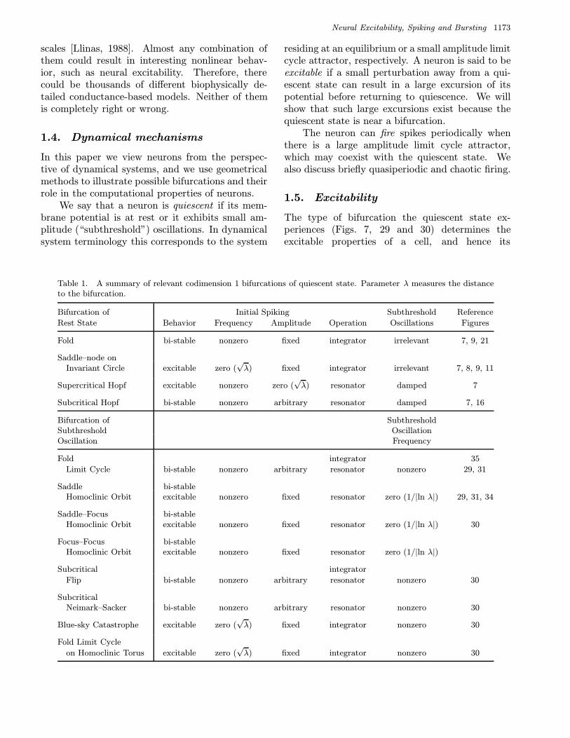
Table 1. A summary of relevant codimension 1 bifurcations of quiescent state. Parameter λ measures the distanceto the bifurcation.
Bifurcation of Initial Spiking Subthreshold Reference
Rest State Behavior Frequency Amplitude Operation Oscillations Figures
Fold bi-stable nonzero fixed integrator irrelevant 7, 9, 21
Saddle–node onInvariant Circle excitable zero (
√λ) fixed integrator irrelevant 7, 8, 9, 11
Supercritical Hopf excitable nonzero zero (√λ) resonator damped 7
Subcritical Hopf bi-stable nonzero arbitrary resonator damped 7, 16
Bifurcation of SubthresholdSubthreshold OscillationOscillation Frequency
Fold integrator 35
Limit Cycle bi-stable nonzero arbitrary resonator nonzero 29, 31
Saddle bi-stableHomoclinic Orbit excitable nonzero fixed resonator zero (1/|ln λ|) 29, 31, 34
Saddle–Focus bi-stableHomoclinic Orbit excitable nonzero fixed resonator zero (1/|ln λ|) 30
Focus–Focus bi-stableHomoclinic Orbit excitable nonzero fixed resonator zero (1/|ln λ|)
Subcritical integrator
Flip bi-stable nonzero arbitrary resonator nonzero 30
SubcriticalNeimark–Sacker bi-stable nonzero arbitrary resonator nonzero 30
Blue-sky Catastrophe excitable zero (√λ) fixed integrator nonzero 30
Fold Limit Cycle
on Homoclinic Torus excitable zero (√λ) fixed integrator nonzero 30

1174 E. M. Izhikevich
neuro-computational attributes. For example,
• When the rest state is near a saddle–node on in-variant circle bifurcation, the neuron can fire all-or-none spikes with an arbitrary low frequency,it has a well-defined threshold manifold, it candistinguish between excitatory and inhibitory in-put, and it acts as an integrator ; i.e. the higherthe frequency of incoming spikes, the sooner itfires.• When the rest state is near an Andronov–Hopf bi-
furcation, the neuron fires in a certain frequencyrange, it does not have all-or-none spikes, it doesnot have a well-defined threshold manifold, it canfire in response to an inhibitory pulse, and it actsas a resonator ; i.e. it responds preferentially toa certain (resonant) frequency of the input. In-creasing the input frequency may actually delayor terminate its firing.
We discuss neural excitability in Sec. 2 andsummarize some basic results in Table 1.
1.6. Periodic spiking
Neuro-computational properties of cells also dependon bifurcations of large amplitude limit cycles corre-sponding to periodic spiking. In general, such bifur-cations differ from bifurcations of quiescent states:For example, when the limit cycle is about to disap-pear via a saddle homoclinic orbit, a fold limit cyclebifurcation, or it loses stability through a subcrit-ical flip or Neimark–Sacker bifurcation, it coexistswith a stable quiescent state. Hence a weak per-turbation having appropriate timing can shut downperiodic spiking prematurely. We discuss these andother issues in Sec. 3 and summarize some majorresults in Table 2.
1.7. Bursting
When neuron activity alternates between a quies-cent state and repetitive spiking, the neuron activ-ity is said to be bursting ; see Fig. 1. It is usuallycaused by a slow voltage- or calcium-dependent pro-cess that can modulate fast spiking activity. There
Table 2. A summary of relevant codimension 1 bifurcations of large amplitude spiking. Parameter λ measuresthe distance to the bifurcation.
Bifurcation ofTerminating Spiking
Periodic Firing Behavior Frequency Amplitude Locking
Saddle–node on Invariant Circle excitable zero (√λ) fixed difficult
Supercritical Hopf excitable nonzero zero (√λ) easy
Fold Limit Cycle bi-stable nonzero arbitrary easy
Saddle Homoclinic Orbit bi-stable zero (1/|ln λ|) fixed easy (?)
Saddle–Focus Homoclinic Orbit bi-stable zero (1/|ln λ|) fixed easy (?)
Focus–Focus Homoclinic Orbit bi-stable zero (1/|ln λ|) fixed easy (?)
Subcritical Flip bi-stable nonzero arbitrary easy
Subcritical Neimark–Sacker bi-stable nonzero arbitrary easy
Blue-sky excitable zero (√λ) fixed difficult
Bifurcation ofQuasi-periodic
Firing
Fold Limit Cycle on
Homoclinic Torus excitable zero (√λ) fixed difficult

Neural Excitability, Spiking and Bursting 1175
Bursting
V(t)
Bifurcationof rest state
Bifurcationof limit cycle
Fig. 2. Two important bifurcations associated withbursting.
are two important bifurcations (see Fig. 2) associ-ated with bursting:
• Bifurcation of a quiescent state that leads torepetitive spiking; see left column in Table 3.• Bifurcation of a spiking attractor that leads to
quiescence; see top row in Table 3.
We restrict our consideration to bifurcations ofcodimension 1, since they are the most probableto be encountered in nature.
We refer to a burster as being a point–cyclewhen the quiescent state is an equilibrium point andthe spiking state is a limit cycle. When the quies-cent state is a small amplitude (subthreshold) oscil-lation, then the burster is said to be cycle–cycle.
We refer to a burster as being planar whenthe fast spiking subsystem is two-dimensional.This imposes severe restriction on possible bifurca-tions. Table 3 summarizes 24 planar codimension 1
bursters. We name them after the two bifurcationsinvolved. Among them are 16 point–cycle and 8cycle–cycle bursters, which are in the upper andlower parts of the table, respectively. We discussthem in detail in Sec. 4.
A complete classification of all 16 planar point–cycle bursters, though without the naming scheme,was first provided by Hoppensteadt and Izhikevich[1997, Sec. 2.9]. Among them were the well-known
• “Fold/homoclinic” burster, also known as“square-wave” or Type I burster.• “Circle/circle” burster, also known as “parabolic”
or Type II burster.• “SubHopf/fold cycle” burster, also known as “el-
liptic” or Type III burster.• “Fold/fold cycle” burster, also known as Type IV
burster.• “Fold/Hopf” burster, also known as “tapered” or
Type V burster.• “Fold/circle” burster, also known as “triangular”
burster.
Many other bursting types listed in Table 3 are new.We show in Sec. 4 that there could be many morebursters if the fast subsystem is multidimensional.They are classified in Table 4.
The history of formal classification of burst-ing starts from the seminal paper by Rinzel [1987],who contrasted the bifurcation mechanism of the“square-wave”, “parabolic”, and “elliptic” bursters.Then, Bertram et al. [1995] suggested to refer to
Table 3. A classification of codimension 1 planar fast–slow bursters. The upper (lower) part of the table correspondsto point–cycle (cycle–cycle) bursters. See also Table 4 and Figs. 53 and 126.
Saddle–Node Saddleon Invariant Homoclinic Supercritical
Bifurcations Circle Orbit Andronov–Hopf Fold Limit Cycle
Fold fold/circle fold/homoclinic fold/Hopf fold/fold cycle
Saddle–Node on circle/circle circle/homoclinic circle/Hopf circle/fold cycle
Invariant Circle
Supercritical Hopf/circle Hopf/homoclinic Hopf/Hopf Hopf/fold cycle
Andronov–Hopf
Subcritical subHopf/circle subHopf/homoclinic subHopf/Hopf subHopf/fold cycle
Andronov–Hopf
Fold Limit Cycle fold cycle/circle fold cycle/homoclinic fold cycle/Hopf fold cycle/fold cycle
Saddle Homoclinic homoclinic/circle homoclinic/homoclinic homoclinic/Hopf homoclinic/fold cycle
Orbit

1176 E. M. Izhikevich
0.5 0.4 0.3 0.2 0.1 0 0.1 0.2 0.3 0.4 0.50.2
0.1
0
0.1
0.2
0.3
0.4
0.5
0.6
0.7
0.8
V
w
V
V
f(x,y)=0
0.5 0.4 0.3 0.2 0.1 0 0.1 0.2 0.3 0.4 0.50.2
0.1
0
0.1
0.2
0.3
0.4
0.5
0.6
0.7
0.8
V
w
ww
g(x,y)=0
0.5 0.4 0.3 0.2 0.1 0 0.1 0.2 0.3 0.4 0.50.2
0.1
0
0.1
0.2
0.3
0.4
0.5
0.6
0.7
0.8
V
w
Fig. 3. Typical nullclines of planar neural systems. (Shown are nullclines for the Morris–Lecar [1981] model.)
the bursters using Roman numbers, and they addeda new, Type IV type. Another, “tapered” typeof bursting was studied simultaneously and inde-pendently by Holden and Erneux [1993a, 1993b],Smolen et al. [1993], and Pernarowski [1994]. Laterde Vries [1998] suggested to refer to it as Type Vburster. Yet another, “triangular” type of burst-ing was studied by Rush and Rinzel [1994], mak-ing the total number of identified bursters to be6. Their bifurcation mechanisms are summarized inFig. 126.
There is a drastic difference between our ap-proach to classification of bursting, and that of thescientists mentioned above. They use a bottom–upapproach; that is, they consider biophysically plau-sible conductance-based models describing experi-mentally observable cellular behavior and then theytry to determine the type of bursting these modelsexhibit. In contrast, we use the top–down approach:We consider all possible pairs of codimension 1 bi-furcations of rest and spiking states, which resultin different types of bursting, and then we invent aconductance-based model exhibiting each burstingtype. Thus, many of our bursters are “theoretical”in the sense that they have yet to be seen in exper-iments. We return to this issue in Sec. 6.1.
1.8. Nullclines and phaseplane analysis
We keep our exposition of bifurcations in neurondynamics as general as possible. Although we usebiophysically detailed Hodgkin–Huxley type neuralmodels to illustrate many issues, most of our bi-furcation diagrams and phase portraits are not re-lated to any specific system of equations. Thus,we emphasize the essentials and omit irrelevantdetails.
Most of the bifurcations discussed here can beillustrated using a two-dimensional (planar) system
of the form
µx = f(x, y)
y = g(x, y) .
Much insight into the behavior of such systems canbe gained by considering their nullclines, i.e. thesets determined by the conditions f(x, y) = 0 org(x, y) = 0; see Fig. 3. When 0 < µ 1, null-clines are called fast and slow, respectively. Sincethe language of nullclines is universal in many areasof applied mathematics, we depict them (as greencurves) in most illustrations.
1.9. The canonical model approach
Whenever possible, we use canonical models toillustrate neuron dynamics. Briefly, a model iscanonical for a family of dynamical systems if everymember of the family can be transformed into themodel by a piecewise continuous possibly noninvert-ible change of variables; see Fig. 4. The definition ofa canonical model generalizes the notions of topo-logical normal form and versal unfolding, and it isdiscussed in detail in Chapter 4 in [Hoppensteadt& Izhikevich, 1997], where one can find many ex-amples of canonical models for neuroscience.
The advantage of considering a canonical modellies in its universality since the model provides in-formation about behavior of the entire family. Forexample, the canonical model (2) describes the dy-namics of any Class 1 excitable neuron regardless ofthe peculiarities of equations one chooses to modelits activity. That is, if one modifies equations andadds more variables and parameters to take intoaccount more ions, currents, pumps, etc., but themodel still exhibits Class 1 excitability, then it stillcan be converted into the canonical model (2) bya (possibly different) change of variables. Thus,taking into account more biological data does notchange the form of the canonical model (2), but

Neural Excitability, Spiking and Bursting 1177
h1
x'=f1(x) x'=f2(x) x'=f3(x) x'=f4(x)
h2 h3 h4
y'=g(y)
Neuron
CanonicalModel
Family of Models
Fig. 4. A model y′ = g(y) is canonical for the family of neural models, if each member of the family can be transformed intoy′ = g(y) by a piecewise continuous change of variables.
may only refine our knowledge of possible values ofthe parameter r in the model.
2. Neural Excitability
Consider a system having a stable equilibrium thatis a global attractor. According to the intuitive def-inition of excitability, small perturbations near theequilibrium can cause large excursions for the solu-tion before it returns to the equilibrium. In dynam-ical system terminology this corresponds to a large-amplitude trajectory that starts and ends near theequilibrium; see Figs. 5 and 101. Such a trajectoryis referred to as being a periodic pseudo-orbit, andthe word “pseudo” is used to stress that the endpoints x(t1) and x(t2) are near but not equal to eachother. If x(t1) = x(t2), then the word “pseudo”should be dropped.
Thus, according to our definition, a dynami-cal system having a stable equilibrium is excitableif there is a large amplitude periodic pseudo-orbitpassing near the equilibrium, as in Fig. 5. How largeis “large” and how near is “near” depends on thecontext. Such periodic pseudo-orbit exists becausethe dynamical system is near a bifurcation. Indeed,a small perturbation of the vector field can cause
the end points x(t1) and x(t2) to coalesce, therebycreating a periodic orbit, which corresponds torepetitive spiking. Thus, neurons are excitable be-cause they are near a bifurcation (transition) fromquiescence to repetitive firing.
Now suppose the equilibrium is not a global at-tractor, but has certain domain of attraction. Thenwe say that the system is excitable if the bound-ary of attraction is near the equilibrium. As in theprevious case, small perturbations near the equi-librium can cause large excursions for the solution,but the solution does not return to the equilibrium.It is easy to see that such a neuron is also near abifurcation, because a small perturbation of the vec-tor field can cause the equilibrium to approach itsboundary of attraction, resulting in loss of stabilityor disappearance.
Hodgkin’s Classification of Excitability. Asimple but useful criterion for classifying excitabil-ity was suggested by Hodgkin [1948]. He stimulateda cell by applying currents of various strengths.When the current is weak the cell is quiet. Whenthe current is strong enough, the cell starts to firerepeatedly; see Fig. 6.

1178 E. M. Izhikevich
Morris-Lecar Hodgkin-Huxley
12x(t )
x(t )
2x(t )
1x(t )
Hodgkin-HuxleyBoundary ofAttraction
Fig. 5. A system is excitable when the rest state has a periodic pseudo-orbit (blue) or the boundary of attraction domain(yellow) is near the rest state. (A periodic pseudo-orbit is a piece of solution x(t), t ∈ [t1; t2] such that x(t1) is near x(t2).)
0 100 200 300 400 500 600 700 800 900 1000
0
0.2
0 100 200 300 400 500 600 700 800 900 1000
0
20
0.6
0.9
7.5
17.5
Morris-Lecar Hodgkin-Huxley
Spi
king
Fre
quen
cy
Spi
king
Fre
quen
cy
II
V(t)V(t)
Class 1 Neural Excitability Class 2 Neural Excitability
I I
I
V(t)
Fig. 6. Transition from rest to repetitive spiking in two biophysical models when the strength of applied current, I, increases.(Noise is added to the Hodgkin–Huxley system to reduce the slow passage effect.)
He divided neurons into two classes accordingto the frequency of emerging firing:
• Class 1 neural excitability. Action potentialscan be generated with arbitrarily low frequency.The frequency increases with increasing the ap-plied current.• Class 2 neural excitability. Action potentials
are generated in a certain frequency band that isrelatively insensitive to changes in the strength ofthe applied current.
Class 1 excitable neurons fire at frequencies thatvary smoothly over a range of about 5–150 Hz. Thefrequency band of the Class 2 excitable neurons isusually in the range 75–150 Hz, but these bandscan vary from neuron to neuron. The exact num-
bers are not important to us here. The qualitativedistinction between Class 1 and Class 2 excitableneurons is that the emerging oscillations have zerofrequency in the former and nonzero frequency inthe latter. This reflects different underlying bifur-cation mechanisms.
Possible Bifurcations. The first attemptto classify excitability using dynamical sys-tems belongs to FitzHugh [1955], although hedid not use the bifurcation theory explicitly.In what follows we use the approach sug-gested by Rinzel and Ermentrout [1989] andconsider the strength of applied current inHodgkin’s experiments as being a quasistatic bi-furcation parameter. When the current increases,
Neural Excitability, Spiking and Bursting 1179
Saddle-Node on Invariant Circle
Fold (off Limit Cycle)
Supercritical Andronov-Hopf
Subcritical Andronov-Hopf
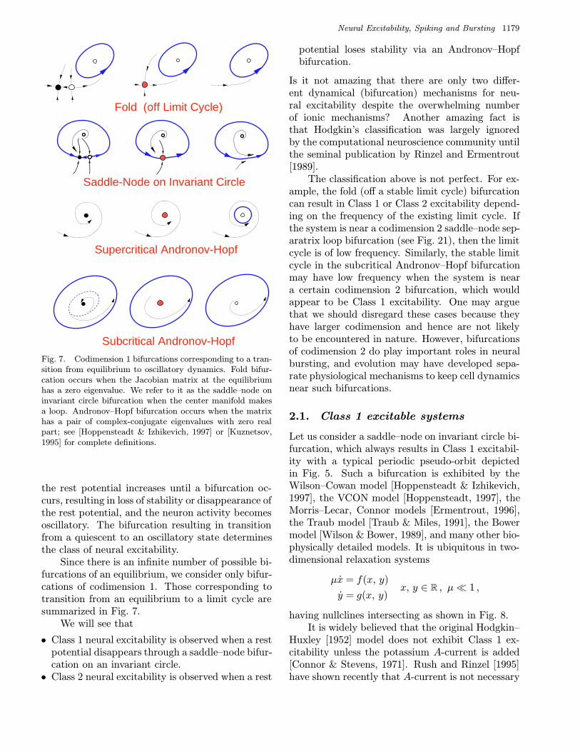
Fig. 7. Codimension 1 bifurcations corresponding to a tran-sition from equilibrium to oscillatory dynamics. Fold bifur-cation occurs when the Jacobian matrix at the equilibriumhas a zero eigenvalue. We refer to it as the saddle–node oninvariant circle bifurcation when the center manifold makesa loop. Andronov–Hopf bifurcation occurs when the matrixhas a pair of complex-conjugate eigenvalues with zero realpart; see [Hoppensteadt & Izhikevich, 1997] or [Kuznetsov,1995] for complete definitions.
the rest potential increases until a bifurcation oc-curs, resulting in loss of stability or disappearance ofthe rest potential, and the neuron activity becomesoscillatory. The bifurcation resulting in transitionfrom a quiescent to an oscillatory state determinesthe class of neural excitability.
Since there is an infinite number of possible bi-furcations of an equilibrium, we consider only bifur-cations of codimension 1. Those corresponding totransition from an equilibrium to a limit cycle aresummarized in Fig. 7.
We will see that
• Class 1 neural excitability is observed when a restpotential disappears through a saddle–node bifur-cation on an invariant circle.• Class 2 neural excitability is observed when a rest
potential loses stability via an Andronov–Hopfbifurcation.
Is it not amazing that there are only two differ-ent dynamical (bifurcation) mechanisms for neu-ral excitability despite the overwhelming numberof ionic mechanisms? Another amazing fact isthat Hodgkin’s classification was largely ignoredby the computational neuroscience community untilthe seminal publication by Rinzel and Ermentrout[1989].
The classification above is not perfect. For ex-ample, the fold (off a stable limit cycle) bifurcationcan result in Class 1 or Class 2 excitability depend-ing on the frequency of the existing limit cycle. Ifthe system is near a codimension 2 saddle–node sep-aratrix loop bifurcation (see Fig. 21), then the limitcycle is of low frequency. Similarly, the stable limitcycle in the subcritical Andronov–Hopf bifurcationmay have low frequency when the system is neara certain codimension 2 bifurcation, which wouldappear to be Class 1 excitability. One may arguethat we should disregard these cases because theyhave larger codimension and hence are not likelyto be encountered in nature. However, bifurcationsof codimension 2 do play important roles in neuralbursting, and evolution may have developed sepa-rate physiological mechanisms to keep cell dynamicsnear such bifurcations.
2.1. Class 1 excitable systems
Let us consider a saddle–node on invariant circle bi-furcation, which always results in Class 1 excitabil-ity with a typical periodic pseudo-orbit depictedin Fig. 5. Such a bifurcation is exhibited by theWilson–Cowan model [Hoppensteadt & Izhikevich,1997], the VCON model [Hoppensteadt, 1997], theMorris–Lecar, Connor models [Ermentrout, 1996],the Traub model [Traub & Miles, 1991], the Bowermodel [Wilson & Bower, 1989], and many other bio-physically detailed models. It is ubiquitous in two-dimensional relaxation systems
µx = f(x, y)
y = g(x, y)x, y ∈ R , µ 1 ,
having nullclines intersecting as shown in Fig. 8.It is widely believed that the original Hodgkin–
Huxley [1952] model does not exhibit Class 1 ex-citability unless the potassium A-current is added[Connor & Stevens, 1971]. Rush and Rinzel [1995]have shown recently that A-current is not necessary

1180 E. M. Izhikevich
Rest State
Threshold
Rest State Threshold
Bifurcation
Bifurcation
RepetitiveSpiking
RepetitiveSpiking
Fig. 8. Saddle–node on invariant circle bifurcation in two-dimensional relaxation systems (from [Hoppensteadt & Izhikevich,1997].
for Class 1 excitability if the sodium and potassium(in)activation curves in the Hodgkin–Huxley modelare shifted appropriately.
2.1.1. Threshold
Whenever a bifurcation involves a saddle, the sys-tem has a well-defined threshold — the stable man-ifold of the saddle [FitzHugh, 1955], which is of-ten referred to as a separatrix since it separatesinto two regions of the phase space having differ-ent qualitative behavior. Indeed, small perturba-tions of the solution that do not lead beyond theseparatrix in Fig. 9 decay, while those crossing itgrow away exponentially thereby producing a spike.Such a system is said to have all-or-none behavior.Because the solution eventually returns to the sta-ble node (rest point), the system is not oscillatory,but excitable.
Notice that the threshold is a codimension 1manifold, which can be a point only when the sys-tem is one-dimensional. Thus, it is futile to seeka threshold value of the membrane voltage, unlessthere is a way to freeze all the other variables.
2.1.2. Canonical model for Class 1excitable systems
When the saddle and node in Fig. 8 coalesce anddisappear, the vector field remains small at the lo-cation of the saddle–node point. Therefore, thesolution (x(t), y(t)) spends most time near thatpoint, then makes a relatively fast excursion, orspike. This observation lays the basis for prov-ing the Ermentrout–Kopell Theorem for Class 1
Spike
Rest State Threshold(Separatrix)
Fig. 9. Excitable behavior and a threshold at fold (saddle–node) bifurcation.
Neural Excitability [Hoppensteadt & Izhikevich,1997, Theorem 8.3].
Theorem 1. (Ermentrout–Kopell). A family ofdynamical systems of the form
x = f(x, λ) , x ∈ Rm , λ ∈ R , (1)
having a saddle–node on invariant circle bifurcationfor λ = 0 has a nonlocal canonical model
ϑ′ = (1− cos ϑ) + (1 + cos ϑ)r , (2)
plus higher-order terms in λ, where ′ = d/dτ , τ =√|λ|t is slow time, ϑ ∈ S1 is a canonical variable
along the invariant circle, and r ∈ R is some pa-rameter that depends on f and λ. That is, thereis an open O(1)-neighborhood, W, of the invariantcircle and a mapping h : W → S1 that projects allsolutions of (1) to those of (2).
The mapping h : W → S1 blows up a smallneighborhood of the saddle–node point and com-presses the entire invariant circle to an open set

Neural Excitability, Spiking and Bursting 1181
xθh
0πR Sm 1
Fig. 10. The transformation h maps solutions of (1) to thoseof (2) (from [Izhikevich, 1999b]).
0πSpike
RestPotential
ThresholdPotential
AbsoluteRefractory
Relative Refractory
Excited(Regenerative)
θ
θ+
−
S1
Fig. 11. Physiological diagram of the canonical model (2)for Class 1 neural excitability (from [Hoppensteadt & Izhike-vich, 1997]).
around π ∈ S1; see Fig. 10. Thus, when x makesa rotation around the invariant circle (generates aspike), the canonical variable ϑ crosses a tiny openset around π.
The canonical model (2) has a simplebehavior:
• If r < 0, then there are two equilibria
ϑ± = ± cos−1 1 + r
1− rwhich are the rest and threshold states; seeFig. 11. The system is excitable in the follow-ing sense: Small perturbations of ϑ that do notlead beyond the threshold value ϑ+ die out ex-ponentially; in contrast, if ϑ is perturbed beyondthe threshold, it grows further, passes the spikevalue ϑ = π, and only after that returns to therest state ϑ−. The equilibria ϑ− and ϑ+ coalescewhen r → 0.• If r > 0, then there are no equilibria, and ϑ(t) os-
cillates with the frequency ω = 2√r. Hence the
original system (1) oscillates with the frequency2√|λ|r, which has been confirmed by experimen-
tal observations (see [Ermentrout, 1996; Gucken-heimer et al., 1997]).
We see that r plays the role of a bifurcation pa-rameter in (2). When it crosses 0, the qualitativebehavior changes. If r 6= 0, then we can use thechange of variables [Izhikevich, 1999b]
ϕ = 2 atan1√|r|
tanϑ
2(3)
to transform the canonical model into one of thefollowing simple forms
ϕ′ = −ω cos ϕ (excitable activity; r < 0)
ϕ′ = ω (periodic activity; r > 0)
where ω = 2√|r| is a positive parameter. The
transformation (3) justifies the empirical observa-tion that the behavior of the canonical model fornegative r is equivalent to that for r = −1; and forpositive r is equivalent to that for r = +1.
2.1.3. Slow adaptation currents
While deriving the canonical model (2) we implic-itly assume that all ionic processes in (1) occur onthe time scale much faster than the interspike in-terval. To take into account slowly (in-)activatingionic currents, we consider the system
x = f(x, y, λ)
y = µg(x, y) .
If µ = O(|λ|), then this system is not near a saddle–node on invariant circle bifurcation, but near someother bifurcation of large codimension. Neverthe-less, if dynamics of y satisfy some fairly general andbiophysically plausible conditions, such as y = 0 isan exponentially stable equilibrium when x is qui-escent, then one can derive the canonical model
ϑ′ = (1− cos ϑ) + (1 + cos ϑ)(r + su) (4)
u′ = δ(ϑ − π)− ηu (5)
where η 1, and δ is the Dirac delta function.Whenever ϑ crosses π (fires a spike), the slowvariable u experiences a step-like increase, then itslowly relaxes to u = 0. The sign of s determineswhether this firing advances or delays the next fir-ing, which results in spike facilitation or adaptation,respectively. We discuss the latter phenomenon inSec. 3.1.

1182 E. M. Izhikevich
2.1.4. Weakly connected networks
The canonical model (2) is probably the simplestexcitable system in mathematical neuroscience: Itis one-dimensional,1 it has Class 1 neural excitabil-ity or periodic activity, and it is biologically plau-sible in the sense that any other Class 1 excitableneuro-system can be converted to the form (2) by anappropriate change of variables. It is not surprisingthat it can be generalized [Hoppensteadt & Izhike-vich, 1997; Izhikevich, 1999b] to a weakly connectednetwork of Class 1 excitable neurons
xi = fi(xi, λ) + εn∑j=1
gij(xi, xj, λ, ε) (6)
where ε 1 measures the strength of connections.
Theorem 2. Suppose the system (6) satisfies thefollowing two conditions
• Each subsystem
xi = fi(xi, λ) (7)
has a saddle–node bifurcation on an invariant cir-cle for λ = 0.• Each function gij = 0 when xj is in some small
neighborhood of the rest state.
Then there is an ε0 > 0 such that for all ε ε0 thefamily (6) has one of the following canonical mod-els depending on the relative magnitudes of |λ| andε (see Fig. 12).
Case 1. |λ| ε2.
ϑ′i = (1− cos ϑi) + (1 + cos ϑi)ri
+n∑j=1
wij(ϑi)δ(ϑj − π) (8)
where δ is the Dirac delta function, each functionwij has the form
wij(ϑi) = 2 atan
(tan
ϑi2
+ sij
)− ϑi , (9)
see Fig. 13, and each sij is a constant.
ε
|λ|
Distance toBifurcation
O (ε) O (ε )2
Strength of Connections
Case 1
Case 2
Case 3
Fig. 12. A weakly connected network of Class 1 excitableneurons (6) has various canonical models depending on therelative sizes of λ and ε (from [Izhikevich, 1999b]).
2
0−π +πθ
w
i
ij
Fig. 13. A typical graph of the function (9). (Here sij = 1.From [Izhikevich, 1999b].)
Case 2. ε2 |λ| ε.
ϑ′i=(1−cos ϑi)+(1+cos ϑi)
ri+ n∑j=1
sijδ(ϑj−π)
(10)
Case 3. |λ| ε and subsystems (7) have limitcycles with equal frequency.
ϕ′i = ωi +n∑j=1
sijH(ϕj − ϕi) , H(χ) = 1− cos χ ,
(11)
The canonical phase model (11) differs from theKuramoto model, which has H(χ) = sin χ.
Systems (9) and (10) are pulse-coupled neuralnetworks in the sense that they are uncoupled un-less at least one ϑj crosses π; i.e. it fires a spike. Thisevent produces a step-like increase in other variablesdue to the term containing Dirac’s delta function.Unlike the standard integrate-and-fire model, themagnitude of the pulse is not a constant, but itdepends on the current state of the post-synapticneuron.
1More precisely, it is defined on a one-dimensional manifold S1.
Neural Excitability, Spiking and Bursting 1183
2.1.5. Slowly connected networks
When we consider weakly connected systems of theform (6) we implicitly assume that synaptic trans-mission is relatively fast in comparison with the in-terspike period. To study the case of slow transmis-sion, we consider the system of the form
xi = fi(xi, λ) + εn∑j=1
gij(xi, yj)
yi = µpi(xi, yi)
where the vector yi describes slow synaptic pro-cesses. We require that yi = 0 be an exponentiallystable equilibrium when xi is quiescent. The canon-ical model for the system above is derived elsewhere,and it has the form
ϑ′i = (1− cos ϑi) + (1 + cos ϑi)
ri +n∑j=1
sijwj
w′i = δ(ϑj − π)− ηwi
where η = O(µ/√|λ|). The term siiwi denotes not
a self-synapse, but a slow adaptation (sii < 0) orfacilitation (sii > 0) process.
A remarkable fact is that ε does not have tobe small for the derivation to be valid. This col-laborates the well-known principle that strongly butslowly connected systems are similar to weakly con-nected systems in many respects [Frankel & Kiemel,1993].
2.1.6. Class 1 excitable neuronsare integrators
Consider the canonical model (8) or (10) and sup-pose that sij > 0, which corresponds to excitatory
synapse. Then both wij(ϑi) and (1 + cos ϑi) arenon-negative for any ϑi. Thus, each incoming spikeadvances ϑi toward π. The higher the frequencyof incoming spikes, the sooner ϑi will reach π and“fire”. This important “integrate-and-fire” featuremakes Class 1 excitable systems integrators. In con-trast, we will show that Class 2 excitable systemsmay act as resonators; i.e. they respond preferen-tially to certain resonant frequencies of the input.
2.1.7. Post-inhibitory spikes
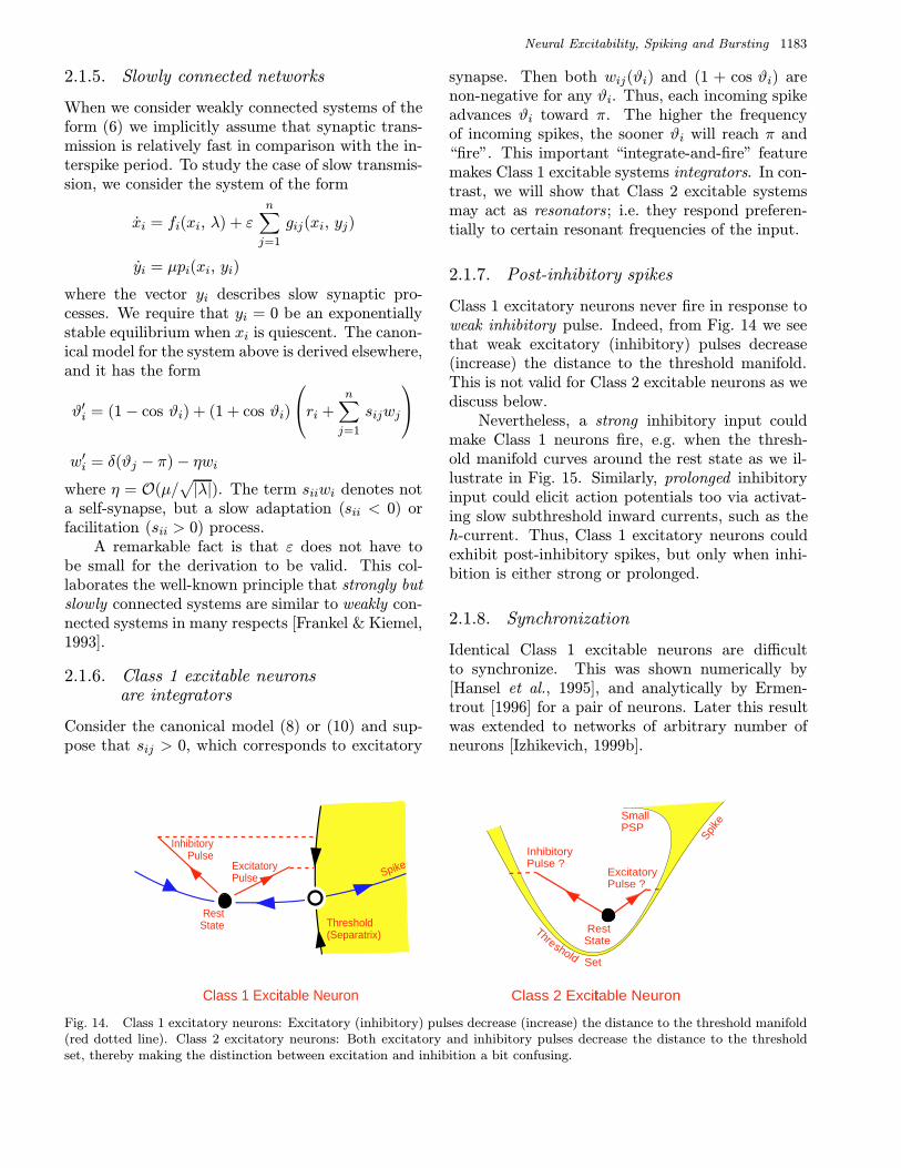
Class 1 excitatory neurons never fire in response toweak inhibitory pulse. Indeed, from Fig. 14 we seethat weak excitatory (inhibitory) pulses decrease(increase) the distance to the threshold manifold.This is not valid for Class 2 excitable neurons as wediscuss below.
Nevertheless, a strong inhibitory input couldmake Class 1 neurons fire, e.g. when the thresh-old manifold curves around the rest state as we il-lustrate in Fig. 15. Similarly, prolonged inhibitoryinput could elicit action potentials too via activat-ing slow subthreshold inward currents, such as theh-current. Thus, Class 1 excitatory neurons couldexhibit post-inhibitory spikes, but only when inhi-bition is either strong or prolonged.
2.1.8. Synchronization
Identical Class 1 excitable neurons are difficultto synchronize. This was shown numerically by[Hansel et al., 1995], and analytically by Ermen-trout [1996] for a pair of neurons. Later this resultwas extended to networks of arbitrary number ofneurons [Izhikevich, 1999b].
Spike
RestState Threshold
(Separatrix)
ExcitatoryPulse
InhibitoryPulse
Class 1 Excitable Neuron
RestState
Spike
ExcitatoryPulse ?
InhibitoryPulse ?
Class 2 Excitable Neuron
shold Set
Thre
SmallPSP
Fig. 14. Class 1 excitatory neurons: Excitatory (inhibitory) pulses decrease (increase) the distance to the threshold manifold(red dotted line). Class 2 excitatory neurons: Both excitatory and inhibitory pulses decrease the distance to the thresholdset, thereby making the distinction between excitation and inhibition a bit confusing.

1184 E. M. Izhikevich
Threshold(Separatrix)
StrongPulse
Fig. 15. A strong inhibitory input can elicit spike in Class 1excitable neuron when the threshold manifold curves aroundthe rest state.
Indeed, consider the phase model (11) and sup-pose that ω1 = ω2 and s12 = s21 = 1. Then, thephase difference, χ = ϕ2 − ϕ1, satisfies
χ′ = H(−χ)−H(χ) ≡ 0 .
because H(χ) = 1− cos χ is an even function. Thisprevents stable synchronization, at least on the timescale of order 1/ε. In contrast, Class 2 excitable sys-tems near supercritical Andronov–Hopf bifurcationhave
H(χ) = sin(χ− ψ) ,
where ψ ∈ S1 is some parameter that has the mean-ing of the natural phase difference [Hoppensteadt& Izhikevich, 1996] because χ → ψ in the unidi-rectional case. If ψ 6= ±π/2, then such systemsalways synchronize stably. Whether or not this factcan be extended to all Class 2 excitable and spikingsystems is still unknown, although numerous simu-lations suggest so.
2.2. Class 2 excitable systems near anAndronov Hopf bifurcation
The Andronov–Hopf bifurcation was thought to bethe primary bifurcation of the rest potential in neu-rons because it is a primary route from rest tooscillations in the Hodgkin–Huxley model, whichis one of the most significant models in computa-tional neuroscience. As a result, this bifurcationhas been scrutinized numerically and analyticallyby many researches (see e.g. [Hassard, 1978; Troy,1978; Rinzel & Miller, 1980; Hassard et al., 1981;Holden et al., 1991; Bedrov et al., 1992]).
A remarkable historical fact is that many im-portant neuroscience properties, such as all-or-noneresponse, threshold, and integration, have been
introduced or illustrated using classical Hodgkin–Huxley model despite the fact that the model doesnot exhibit any of these properties, as we see below.
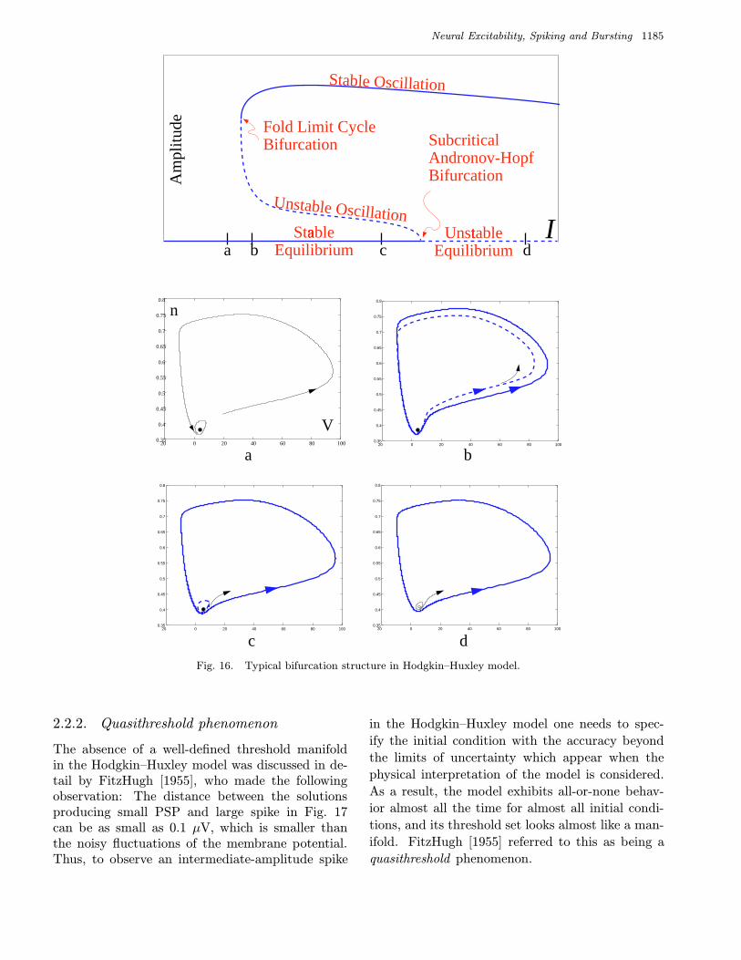
The Hodgkin–Huxley model, as well as manyother biophysical models, has a typical bifurcationstructure as depicted in Fig. 16. While the bifur-cation parameter I increases, stable and unstablelimit cycles appear via fold limit cycle bifurcation.The latter shrinks down to the rest state and makesit lose stability via subcritical Andronov–Hopfbifurcation.
At any value of I the phase portrait is equiv-alent to that of the topological normal form fora Bautin bifurcation [Kuznetsov, 1995; Izhikevich,2000a]
z′ = (a+ iω) + bz|z|2 − z|z|4 , z ∈ C , (12)
Apart from qualitative illustration of bifurcationsin Hodgkin–Huxley-type systems, the model abovemay be of limited value since it fails to reflect therelaxation nature of the dynamics.
2.2.1. Threshold, excitability, and bistability
An important consequence of relaxation dynamicsis that the flow can undergo large contractions andexpansions. For example, the stable and unsta-ble limit cycles in Fig. 16(b) are so close to eachother when they are near an equilibrium, that theycould become indistinguishable if small noise is in-troduced into the system.
Figures 16(b) and 16(c) illustrate the bistablenature of dynamics of the Hodgkin–Huxley model.The unstable limit cycle separates the basins ofattraction of the rest state and the large ampli-tude limit cycle corresponding to repetitive spik-ing. Therefore, the unstable cycle is a thresholdmanifold.
When the equilibrium is a global attractor, asin Fig. 16(a), a small perturbation of a solution nearthe equilibrium can still produce a large deviation;see Fig. 17. Therefore, the system is excitable witha typical periodic pseudo-orbit depicted in Fig. 5.However, a threshold manifold may not exist. In-deed, if the initial condition lies in the yellow re-gion between the two solutions in the right inlet inFig. 17, the system can produce a spike having anarbitrary intermediate amplitude. We refer to theregion as being a threshold set. We see that theHodgkin–Huxley model does not have all-or-noneresponse.
Neural Excitability, Spiking and Bursting 1185
20 0 20 40 60 80 1000.35
0.4
0.45
0.5
0.55
0.6
0.65
0.7
0.75
0.8
20 0 20 40 60 80 1000.35
0.4
0.45
0.5
0.55
0.6
0.65
0.7
0.75
0.8
20 0 20 40 60 80 1000.35
0.4
0.45
0.5
0.55
0.6
0.65
0.7
0.75
0.8
20 0 20 40 60 80 1000.35
0.4
0.45
0.5
0.55
0.6
0.65
0.7
0.75
0.8
V
n
I
Am
plit
ude
a
b
c d
dc
a
b
Fold Limit CycleBifurcation Subcritical
Andronov-HopfBifurcation
Stable Oscillation
Unstable OscillationStable
EquilibriumUnstable
Equilibrium
Fig. 16. Typical bifurcation structure in Hodgkin–Huxley model.
2.2.2. Quasithreshold phenomenon
The absence of a well-defined threshold manifoldin the Hodgkin–Huxley model was discussed in de-tail by FitzHugh [1955], who made the followingobservation: The distance between the solutionsproducing small PSP and large spike in Fig. 17can be as small as 0.1 µV, which is smaller thanthe noisy fluctuations of the membrane potential.Thus, to observe an intermediate-amplitude spike
in the Hodgkin–Huxley model one needs to spec-
ify the initial condition with the accuracy beyond
the limits of uncertainty which appear when the
physical interpretation of the model is considered.
As a result, the model exhibits all-or-none behav-
ior almost all the time for almost all initial condi-
tions, and its threshold set looks almost like a man-
ifold. FitzHugh [1955] referred to this as being a
quasithreshold phenomenon.
1186 E. M. Izhikevich
Threshold Set
Spike
SmallPSP
Fig. 17. Neural systems near Andronov–Hopf bifurcationmay not have a well-defined threshold. Depicted are two“nearby” solutions of the Hodgkin–Huxley system fromFig. 16(a). One corresponds to a small amplitude postsynap-tic potential (PSP), while the other evolves into an actionpotential.
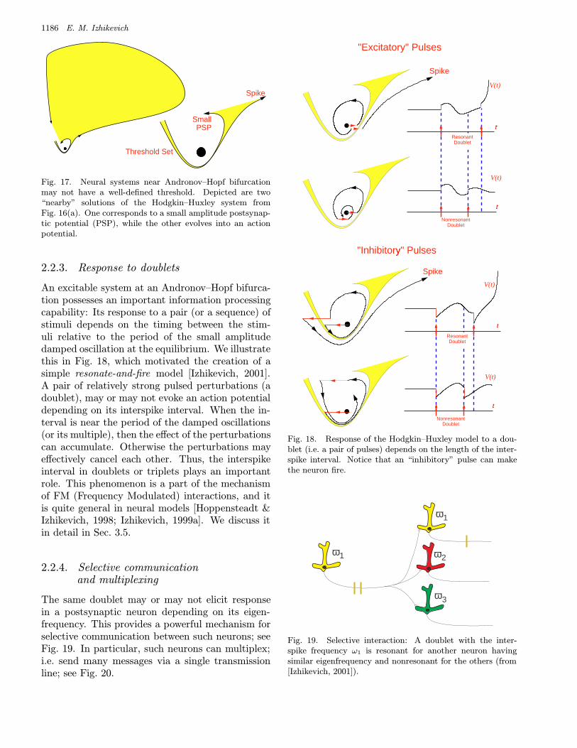
2.2.3. Response to doublets
An excitable system at an Andronov–Hopf bifurca-tion possesses an important information processingcapability: Its response to a pair (or a sequence) ofstimuli depends on the timing between the stim-uli relative to the period of the small amplitudedamped oscillation at the equilibrium. We illustratethis in Fig. 18, which motivated the creation of asimple resonate-and-fire model [Izhikevich, 2001].A pair of relatively strong pulsed perturbations (adoublet), may or may not evoke an action potentialdepending on its interspike interval. When the in-terval is near the period of the damped oscillations(or its multiple), then the effect of the perturbationscan accumulate. Otherwise the perturbations mayeffectively cancel each other. Thus, the interspikeinterval in doublets or triplets plays an importantrole. This phenomenon is a part of the mechanismof FM (Frequency Modulated) interactions, and itis quite general in neural models [Hoppensteadt &Izhikevich, 1998; Izhikevich, 1999a]. We discuss itin detail in Sec. 3.5.
2.2.4. Selective communicationand multiplexing
The same doublet may or may not elicit responsein a postsynaptic neuron depending on its eigen-frequency. This provides a powerful mechanism forselective communication between such neurons; seeFig. 19. In particular, such neurons can multiplex;i.e. send many messages via a single transmissionline; see Fig. 20.
ResonantDoublet
V(t)
V(t)
t
t
NonresonantDoublet
Spike
"Excitatory" Pulses
ResonantDoublet
V(t)
V(t)
t
t
NonresonantDoublet
Spike
"Inhibitory" Pulses
Fig. 18. Response of the Hodgkin–Huxley model to a dou-blet (i.e. a pair of pulses) depends on the length of the inter-spike interval. Notice that an “inhibitory” pulse can makethe neuron fire.
1ω
1ω
2ω
3ω
Fig. 19. Selective interaction: A doublet with the inter-spike frequency ω1 is resonant for another neuron havingsimilar eigenfrequency and nonresonant for the others (from[Izhikevich, 2001]).

Neural Excitability, Spiking and Bursting 1187
1
2
3
ω
ω
ω
1ω
2ω
3ω
Fig. 20. Multiplexing of neural signals via doublets: Resonate-and-fire neurons having equal eigenfrequencies can interactselectively without any cross interference with other resonate-and-fire neurons (from [Izhikevich, 2001]).
2.2.5. Weak stimulation
Figure 18 is only an illustration, since presynapticpulses do not elicit a step-like increase in membranepotential of postsynaptic Class 2 excitable neurons.They rather induce a weak and relatively slow forc-ing. Nevertheless, the FM mechanism persists, aswe show next.
Let us disregard the global structure of the flowand consider its dynamics in a small neighborhoodof the rest state. We are interested in a responseof the system near the rest state to a weak externalstimulation εI(t) that is due to incoming spikes.
It is well known that any system
x = f(x, ε) , x ∈ Rm
in an ε-neighborhood of the Andronov–Hopf bifur-cation can be reduced to its topological normal form
z = (εa+ iω)z ± z|z|2 , z ∈ C ,
by a continuous transformation. Applying thetransformation to the weakly forced system
x = f(x, ε) + εI(t)
results in
z = εJ(t) + (εa+ iω)z ± z|z|2 (13)
plus higher-order terms, where J(t) ∈ C is a linearprojection of I(t) ∈ Rm. The change of variables
z =√εveiωt , v ∈ C ,
results in the equation
v =√εJ(t)e−iωt + ε(av ± v|v|2) .
We average this system and obtain the equation
v =√εb+ ε(av ± v|v|2) ,
where
b = limT→∞
1
T
∫ T
0J(t)e−iωt dt (14)
is the Fourier coefficient of J(t) corresponding tofrequency ω. The key observation here is that b canvanish even when J(t) 6= 0.
We assume that the equilibrium is stable,i.e. a < 0. If b = 0, then v, and hence x, stay nearthe equilibrium. In contrast, If b 6= 0, then v growslike√εbt until x = O(
√εv) leaves a small neigh-
borhood of the rest state, possibly getting outsideof the unstable limit cycle in Fig. 16(c) and gener-ating a spike.
2.2.6. Class 2 excitable neuronsare resonators
We see that a system near an Andronov–Hopf bifur-cation acts as a bandpass filter: It extracts the com-ponent of the external input I(t) that correspondsto the “resonant” eigenfrequency ω and disregardsthe rest of the spectrum. Thus, in order to evokea response, one should stimulate such a neuron atthe resonant frequency. This behavior has beendescribed in thalamic [Hutcheon et al., 1994; Puilet al., 1994] and cortical neurons [Jansen & Karnup,1994; Gutfreund et al., 1995; Hutcheon et al., 1996].Llinas [1988, 1991] refers to such neurons as beingresonators. In contrast to Class 1 excitable neu-rons, increasing the frequency of stimulation maydelay or even terminate firing of a Class 2 excitableneuron [Izhikevich, 2001], since it may decrease thevalue of |b| defined by (14). We return to this issuein Sec. 3.5 when we discuss FM interactions.

1188 E. M. Izhikevich
2.2.7. Post-inhibitory spike
A salient neuro-computational feature of Class 2excitable neurons is that they can fire in responseto a weak inhibitory pulse (see Fig. 18), which isreferred to as being a post-inhibitory spike. Thismakes the distinction between excitation and inhi-bition a bit confusing, since both can lead to anaction potential. Such a confusion does not exist inClass 1 excitable neurons, because weak excitatory(inhibitory) pulses decrease (increase) the distanceto the threshold manifold; see Fig. 14. Since thethreshold set is always “wrapped” around the reststate of Class 2 excitable neuron, any perturbationwould eventually move the solution closer to the set,thereby facilitating the neuron’s response to otherpulses having appropriate timing.
2.3. Saddle node separatrix-loopbifurcation
Now consider the case of fold (off limit cycle) bi-furcation as in Fig. 17. If the limit cycle is suffi-ciently far away from the saddle–node point, thenits frequency is generically nonzero, and hence sucha bistable system has Class 2 excitability.
Quite often however the limit cycle is near thesaddle–node point, as in Fig. 21. This usually hap-pens when the system is near a codimension 2 bi-furcation called saddle–node separatrix-loop bifur-cation [Levi et al., 1978; Schecter, 1987; Hoppen-steadt, 1997], whose complete unfolding is depictedin Fig. 22. The saddle–node separatrix-loop bifur-cation is typical in two-dimensional systems havingnullclines intersected as in Fig. 23. Such systemsinclude Morris–Lecar, Chay–Cook, and Wilson–Cowan models.
Fold (off Limit Cycle)Bifurcation
Saddle-NodeSeparatrix-Loop Bifurcation
Fig. 21. Fold bifurcation can be near a limit cycle if thesystem is near a saddle–node separatrix loop bifurcation.
Saddle-Node
Separatrix LoopBifurcation
Fig. 22. Unfolding of a codimension 2 saddle–node sepa-ratrix loop bifurcation (from [Hoppensteadt & Izhikevich,1997]).
Fig. 23. Phase portraits from Fig. 22 are typical in two-dimensional systems, such as Wilson–Cowan or Morris–Lecarmodels (modified from [Hoppensteadt & Izhikevich, 1997]).
As we will see in Sec. 4 below, this bifurcationplays an important role in at least four types ofbursting including the “fold/homoclinic” bursting,which is also known as “square-wave” bursting.
2.3.1. Canonical model
It follows from the normally hyperbolic com-pact invariant manifold theory [Fenichel, 1971;

Neural Excitability, Spiking and Bursting 1189
Saddle-Nodeon InvariantCircle
Saddle-NodeSeparatrix Loop
InvariantFoliation
Spike
Fig. 24. A small neighborhood of the saddle–node point canbe invariantly foliated by stable submanifolds.
Hoppensteadt & Izhikevich, 1997, Chap. 4] that asmall neighborhood of the saddle–node point can beinvariantly foliated by stable submanifolds, whichare frequently referred to as being isochrons in thecontext of oscillatory systems; see Fig. 24. Any twodistinct solutions starting on the same submanifoldwill eventually approach each other and have iden-tical asymptotic behavior. This fact was used in theproof of the Ermentrout–Kopell theorem to reducethe dimension of a system.
Now consider a system near a saddle–node sep-aratrix loop bifurcation. All solutions in some smallneighborhood of the saddle–node point (shadedarea in Fig. 24) approach exponentially the centermanifold. A solution on the center manifold slowlydiverges from the equilibrium, makes an excursion(spike) and returns to the neighborhood (shadedarea). But it enters the neighborhood along one ofthe stable submanifolds. The spike occurs when thecanonical variable ϑ in (2) crosses a tiny neighbor-hood of π, but instead of being reset to −π, thevariable ϑ acquires some new value a ∈ S1 that isdetermined by the location of the stable submani-fold that was hit by the separatrix loop; see Fig. 25.
Thus, one can prove under certain natural con-ditions that the canonical model for the saddle–node separatrix-loop bifurcation has the form (2)with the exception that
ϑ(t)← a when ϑ(t) = π .
The parameter r in the canonical model is lo-cal in the sense that it depends on some partialderivatives near the equilibrium [Hoppensteadt &Izhikevich, 1997, Chap. 8]. In contrast, the pa-rameter a is global since it depends on Melnikov’sintegral along the unperturbed separatrix trajec-
Saddle-Nodeon InvariantCircle
Saddle-NodeSeparatrix Loop
SpikeSpikeπ−π
0 0
−ππ
Fig. 25. The saddle–node separatrix loop bifurcation can betreated the same way as the saddle–node on invariant circlebifurcation with the exception that the variable ϑ in (2) isreset to some value a after crossing π.
Spike
Perturbation
Quiescence
Fig. 26. An example of a small amplitude subthresholdoscillation (blue) corresponding to the quiescent state.
tory. The canonical model exhibits a fold bifurca-tion when r = 0, and a saddle homoclinic orbit bi-furcation when r < 0 and cos a = (1+r)/(1−r). Itsbifurcation diagram is similar to the one depictedin Fig. 22, where the a-axis is pointed downward.
2.4. Fast subthreshold oscillations
So far we have considered neuron dynamics at anequilibrium corresponding to the rest (quiescent)state. Next suppose that the membrane potentialhas a fast stable small amplitude “subthreshold”oscillation corresponding to the quiescent state, aswe illustrate in Fig. 26. Such neurons have beenrecorded, e.g. in layer 4 of the guinea pig frontalcortex [Llinas et al., 1991]. Fast subthreshold os-cillations can be seen in conductance-based models[Shorten & Wall, 2000; Wang, 1993].
The simplest and possibly least interesting caseis when the neuron’s activity is always oscillatory ina certain parameter range with an amplitude pro-portional to the external input, as in Fig. 27. Inthis case the distinction between the sub- and super-threshold oscillations may be made by the synap-tic release mechanism; that is, the amplitude of

1190 E. M. Izhikevich
Small External InputNo External Input Large External Input
Fig. 27. The amplitude of oscillation may depend on theexternal input.
Fig. 28. Existence of a large amplitude periodic pseudo-orbit near small amplitude “subthreshold” limit cycle makesthe dynamics excitable.
oscillation is said to be superthreshold if it is largeenough to trigger the release of a neurotransmitterfrom the presynaptic endings.
Notice that small amplitude subthreshold os-cillations do not preclude the system from beingexcitable, since it can still have a large amplitudeperiodic pseudo-orbit; see Fig. 28.
2.4.1. Possible bifurcations
In a more interesting case the small amplitude limitcycle may bifurcate so that some large amplitudelimit cycle corresponding to a periodic spiking be-comes globally stable.
Obviously, the saddle–node on invariant circleand the supercritical Andronov–Hopf bifurcationshould be dismissed as possible bifurcations, sincethey result in a stable equilibrium and not in a largeamplitude limit cycle. Similarly, the supercriticalflip (period doubling) and supercritical Neimark–Sacker bifurcations [Kuznetsov, 1995] should be dis-carded since the newborn attractors lie in a smallneighborhood of the old ones, which is often referredto as a soft loss of stability.
We consider next bifurcations that result insharp loss of stability. These are the fold limit cy-cle and saddle homoclinic orbit bifurcations in theplanar case (see Fig. 29), and the saddle–focus ho-moclinic orbit, subcritical flip, subcritical Neimark–Sacker, fold limit cycle on homoclinic torus, and
Fold Limit Cycle Bifurcation
Saddle Homoclinic Orbit Bifurcation
Fig. 29. Codimension 1 bifurcations of a stable limit cycle inplanar systems that result in sharp loss of stability (see alsoFig. 30). Fold limit cycle: Stable limit cycle is approached byan unstable one, they coalesce, and then disappear. Saddlehomoclinic orbit : A limit cycle grows into a saddle. Unsta-ble manifold of the saddle makes a loop and returns via thestable manifold (separatrix).
the “blue-sky” bifurcations in the three-dimensionalcase; see Fig. 30. The only bifurcation left is thefocus–focus homoclinic orbit, which we do not il-lustrate since it occurs in systems of dimension 4and up; see [Kuznetsov, 1995].
The planar bifurcations are ubiquitous in two-dimensional systems having nullclines intersected asin Fig. 31. Notice the shape of the slow nullcline forthe saddle homoclinic orbit bifurcation. One caneasily modify existing models, such as the van derPol or FitzHugh–Nagumo oscillators, to get suchdynamics. For example, to make Fig. 34 we used
v = v − v3/3− ww = ε(a+ v − S(w))
(15)
where
S(w) =b
1 + e(c−w)/d,
is an S-shaped function. Such a system often ex-hibits the big saddle homoclinic orbit bifurcationdepicted in Fig. 32.
There is a drastic change in the behavior ofthe small limit cycle when the system approachesthe bifurcation state. Its frequency is nonzero forthe fold limit cycle, flip, Neimark–Sacker, blue-sky,and fold limit cycle on homoclinic torus bifurca-tions, and zero for the homoclinic orbit bifurcationssince the cycle becomes a homoclinic trajectory toan equilibrium. This gives a criterion to distin-guish the bifurcations experimentally. Both cases,

Subcritical Neimark-Sacker Bifurcation
Fold Limit Cycle on Homoclinic Torus Bifurcation
Blue-Sky Catastrophe
Saddle-Focus Homoclinic Orbit Bifurcation
Subcritical Flip Bifurcation
Fig. 30. Codimension 1 bifurcations of a stable limit cycle in three-dimensional systems that result in sharp loss of stability(see also Fig. 29). Saddle–focus homoclinic orbit : A limit cycle grows into a saddle–focus and becomes a homoclinic orbit.Subcritical flip: The stable limit cycle is approached by an unstable limit cycle having twice the period, they coalesce, andthe former loses stability. Subcritical Neimark–Sacker : An unstable invariant torus shrinks down to a stable limit cycle. Foldlimit cycle on homoclinic torus: An unstable manifold of a nonhyperbolic limit cycle returns to the cycle forming a homoclinictorus. Blue-sky catastrophe: An unstable manifold of a nonhyperbolic limit cycle becomes a tube and returns to the cycleforming “French horn”; see [Kuznetsov, 1995; Il’iashenko & Li, 1999] for detailed definitions.
1191
1192 E. M. Izhikevich
Fold Limit Cycle Bifurcation
Saddle Homoclinic Orbit Bifurcation
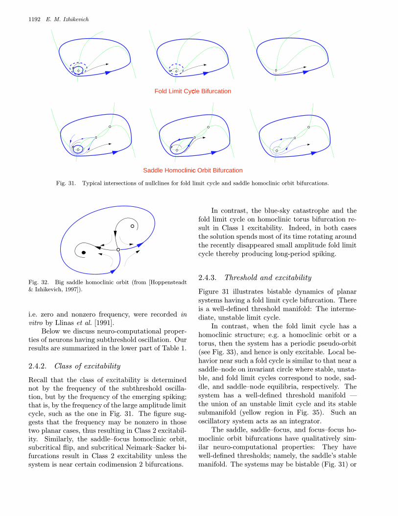
Fig. 31. Typical intersections of nullclines for fold limit cycle and saddle homoclinic orbit bifurcations.
Fig. 32. Big saddle homoclinic orbit (from [Hoppensteadt& Izhikevich, 1997]).
i.e. zero and nonzero frequency, were recorded invitro by Llinas et al. [1991].
Below we discuss neuro-computational proper-ties of neurons having subthreshold oscillation. Ourresults are summarized in the lower part of Table 1.
2.4.2. Class of excitability
Recall that the class of excitability is determinednot by the frequency of the subthreshold oscilla-tion, but by the frequency of the emerging spiking;that is, by the frequency of the large amplitude limitcycle, such as the one in Fig. 31. The figure sug-gests that the frequency may be nonzero in thosetwo planar cases, thus resulting in Class 2 excitabil-ity. Similarly, the saddle–focus homoclinic orbit,subcritical flip, and subcritical Neimark–Sacker bi-furcations result in Class 2 excitability unless thesystem is near certain codimension 2 bifurcations.
In contrast, the blue-sky catastrophe and thefold limit cycle on homoclinic torus bifurcation re-sult in Class 1 excitability. Indeed, in both casesthe solution spends most of its time rotating aroundthe recently disappeared small amplitude fold limitcycle thereby producing long-period spiking.
2.4.3. Threshold and excitability
Figure 31 illustrates bistable dynamics of planarsystems having a fold limit cycle bifurcation. Thereis a well-defined threshold manifold: The interme-diate, unstable limit cycle.
In contrast, when the fold limit cycle has ahomoclinic structure; e.g. a homoclinic orbit or atorus, then the system has a periodic pseudo-orbit(see Fig. 33), and hence is only excitable. Local be-havior near such a fold cycle is similar to that near asaddle–node on invariant circle where stable, unsta-ble, and fold limit cycles correspond to node, sad-dle, and saddle–node equilibria, respectively. Thesystem has a well-defined threshold manifold —the union of an unstable limit cycle and its stablesubmanifold (yellow region in Fig. 35). Such anoscillatory system acts as an integrator.
The saddle, saddle–focus, and focus–focus ho-moclinic orbit bifurcations have qualitatively sim-ilar neuro-computational properties: They havewell-defined thresholds; namely, the saddle’s stablemanifold. The systems may be bistable (Fig. 31) or

Neural Excitability, Spiking and Bursting 1193
Fig. 33. An existence of a large amplitude periodic pseudo-orbit near small amplitude “subthreshold” fold limit cyclemakes the dynamics excitable.
only excitable (Fig. 34) depending on the existenceof an enclosing limit cycle.
Stable limit cycles near subcritical flip andNeimark–Sacker bifurcations also have well-defined
threshold manifolds; namely, the stable submani-fold of unstable double-period cycle and the unsta-ble torus, respectively.
2.4.4. Nonlinear resonators
Neural systems having subthreshold oscillationsmay have an interesting property: Their responseto a brief relatively strong stimulus depends on thetiming of the stimulus relative to the phase of theoscillation. We illustrate this issue in Fig. 34 using(15) near the saddle homoclinic orbit bifurcation. Itis easy to see that the response depends on wherethe solution is on the limit cycle at the time of theperturbation.
There is a similarity between the mechanismsdepicted in Figs. 18 and 34. Both use the fact thata neuron may have its own subthreshold tempo-ral dynamics that affect its response to a perturba-tion. The only difference is that the former cannotoscillate by itself; therefore, it needs a first spiketo evoke a damped subthreshold oscillation whosephase would augment the response to the secondspike.
Threshold(Separatrix)
v(t)
Stimulus
v(t)
Stimulusv
w
Fig. 34. Response of a system having a small amplitude oscillation depends on the timing of the incoming spike relative tothe phase of the subthreshold oscillation.

1194 E. M. Izhikevich
To SpikingLimit Cycle
ThresholdManifoldSubthreshold
Limit Cycle
V
Fig. 35. A system near fold limit cycle bifurcation can stillact as integrator: The effect of perturbations does not dependon the subthreshold oscillation phase. Moreover, increasingthe subthreshold oscillation amplitude does not decrease thedistance to the threshold manifold.
We could have also used any other bifurcations(except blue-sky and homoclinic torus) to illustratethe mechanism depicted in Fig. 34. A distinguishedfeature of the saddle homoclinic orbit bifurcationis that there is an open region above the cycle inFig. 34 such that if perturbations are directed to-ward this region, then they would never elicit aspike regardless of their timing and strength.
Finally, notice that the existence of subthresh-old oscillation does not necessarily imply that thesystem is a resonator, especially when its dimensionis greater than 2. For example, the system near foldlimit cycle bifurcation depicted in Fig. 35 acts asan integrator. Although appropriately timed per-turbations can change the amplitude of oscillation,but such a change does not decrease significantlythe distance to the threshold manifold, and hencedoes not facilitate the spike, see also Fig. 122.
3. Periodic Spiking
So far we have described mechanisms of transitionfrom a quiescent state to repetitive firing; that is,from an equilibrium or a small amplitude limit cy-cle to a large amplitude limit cycle attractor. Howdoes the large attractor arise?
Much insight on possible mechanisms for theappearance of the large attractor can be gainedwhen we consider possible mechanisms of transition
Firi
ng F
requ
ency
I
Firi
ng F
requ
ency
I
Firi
ng F
requ
ency
I
Fre
qu
ency
Ran
ge
Fre
qu
ency
Ran
ge
Fre
qu
ency
Ran
ge
Rest
Spiking
Rest
Spiking
Rest
Class 1Excitable
Class 2Excitable
Class 1Spiking
Class 2Spiking
Class 1Spiking
Class 2Excitable
Spiking
Fig. 36. Class 1 (2) excitable systems exhibit zero (nonzero)emerging spiking. Class 1 (2) spiking systems exhibit zero(nonzero) terminating spiking.
from repetitive spiking to a rest state. FollowingHodgkin’s experiment [1948] we suggest the follow-ing classification of repetitive spiking based on thefrequency as oscillations terminate; see Fig. 36.
• Class 1 Spiking Systems exhibit terminating os-cillations having arbitrary low frequency.• Class 2 Spiking Systems exhibit oscillations that
terminate with a nonzero frequency.
We stress that studying terminating oscillationsprovides a clue about how the attractor correspond-ing to repetitive spiking appears and disappears. Itusually does not provide any information on howthe spiking activity appears. The latter issue isrelated to neural excitability, as discussed in theprevious section.
It is easy to see that a saddle–node on invari-ant circle bifurcation results in a system that is

Neural Excitability, Spiking and Bursting 1195
Cla
ss 2
Exc
itab
ility
Cla
ss 1
Exc
itab
ility
Class 1 SpikingC
lass
1 S
pik
ing
Fig. 37. If the rest state disappears via fold (off limit cycle)bifurcation and the limit cycle disappears via saddle homo-clinic orbit bifurcation (see Fig. 22 for reference), then thesystem is Class 2 excitable but Class 1 spiking.
simultaneously Class 1 excitable and Class 1 spik-ing. Similarly, the supercritical Andronov–Hopf bi-furcation results in a Class 2 excitable and Class 2spiking system. In both cases the transitions fromrest to repetitive firing and back occur via the samebifurcation.
In general, the bifurcation of the rest state maynot be the same as the bifurcation of the limit cy-cle. In this case a stable rest state and a stablelimit cycle coexist making the dynamics bistable,and the class of excitability may not be the sameas the class of spiking. We will present several suchexamples when we discuss bursting.
An example of Class 2 excitable but Class 1spiking system is the fold (off limit cycle) bifurca-tion. If the system is sufficiently away from thecodimension 2 saddle–node separatrix-loop bifurca-tion (see Figs. 22 and 37), then the frequency ofthe limit cycle is not zero at the moment the reststate disappears. This results in Class 2 excitability.The limit cycle can disappear via a saddle–node oninvariant circle or saddle homoclinic orbit bifurca-tion. Both bifurcations are homoclinic, and hencethey result in Class 1 spiking.
Possible Bifurcations. When a repetitive spikingactivity shuts down, the limit cycle attractor eitherloses its stability or disappears. If it loses stabilityvia a soft bifurcation, such as the supercritical flip(period doubling) or supercritical Neimark–Sacker,the new attractor lies in a small neighborhood ofthe old one, so that the system continues to fire but
with a different firing pattern. To shut down thefiring, the loss of stability must be sharp; e.g. via asubcritical flip or subcritical Neimark–Sacker bifur-cations; see Fig. 30.
The large amplitude limit cycle can also disap-pear, for example, via saddle homoclinic orbit orfold limit cycle bifurcation (Fig. 29), saddle–nodeon invariant circle or supercritical Andronov–Hopfbifurcation (Fig. 7), or those from Fig. 30.
We will see that
• Class 1 spiking occurs via saddle–node on invari-ant circle, saddle, saddle–focus, or focus–focushomoclinic orbit, blue-sky, or fold limit cycle onhomoclinic torus bifurcations.• Class 2 spiking occurs via supercritical
Andronov–Hopf, fold limit cycle, subcritical flip,or subcritical Neimark–Sacker bifurcations.
Bifurcations and Current I. The most obviousway to study bifurcations in neuron dynamics is touse the same electrode that measures the membranevoltage to induce the current I, which we treat asa bifurcation parameter. There could be many in-terpretations of the physiological meaning of I. Forexample, we can interpret I as a synaptic current
I = gsyn(Esyn − V ) (16)
or as the current that is due to the difference ofvoltages in soma and dendrites
I = g(Vdendr − V ) ,
etc. Thus, the “actual” bifurcation parameters inthe spiking mechanism are gsyn, Vdendr, etc., butnot I. Therefore, instead of changing I, we shouldslowly change, e.g. gsyn, measure the voltage, andinject I calculated according to (16), which in-volves the dynamic clamp techniques [Sharp et al.,1993; Hutcheon et al., 1996]. Both procedures areequivalent when the membrane potential is at rest,but they may provide quite different bifurcationpictures when the potential oscillates. Thus, oneshould use (16) or its equivalent to study bifurca-tions of spiking limit cycles.
Another potential problem is that the rate ofchange of a bifurcation parameter should be slowenough so that it is treated as a constant by thefast spiking subsystem. Yet it should not be tooslow, or else slow physiological processes start tointerfere and may significantly distort the bifurca-tions picture.

1196 E. M. Izhikevich
0 0.01 0.02 0.03 0.04 0.05 0.06 0.07 0.08 0.090
0.05
0.1
0.15
0.2
0.25
0.3
0.35
0.4
0.45
-1/lnλ
λ
λ
Class 1ExcitableSystems
Class 1SpikingSystems
Fig. 38. The function −1/ ln λ may not seem to vanish asλ→ 0.
3.1. Class 1 spiking systems
Suppose the limit cycle disappears via one of thefollowing bifurcations:
• Saddle–node on invariant circle bifurcation, orblue-sky catastrophe.• Saddle, saddle–focus, or focus–focus homoclinic
orbit bifurcations.
In all these cases the cycle becomes homoclinic toan equilibrium, hence its period goes to infinity, andthe frequency to zero. All these bifurcations resultin Class 1 spiking, but the frequency of terminat-ing oscillations have different asymptotic behavior:The former group’s frequency decays as O(
√λ),
where λ measures the distance to the bifurcation(see Sec. 2.1), while the latter exhibits O(1/| ln λ|).We plot these functions in Fig. 38 to illustrate apossible pitfall: The latter may not seem to van-ish as λ → 0, incorrectly suggesting a frequencycurve for Class 2 spiking system. Thus, extra cau-tion should be used when measuring the functionsexperimentally.
3.1.1. Threshold and bistability
An important difference between the bifurcationsleading to Class 1 spiking is that there may be nocoexistence of attractors at the saddle–node on in-variant circle and blue-sky bifurcations, while thereis at the saddle homoclinic orbit bifurcations. Thus,the former may not result in bistable dynamics.A system is either excitable or oscillatory, and nopulse can shut down the oscillation. In contrast,the latter always result in bistable systems having a
Saddle Homoclinic Orbit
Big Saddle Homoclinic Orbit
Fig. 39. Disappearance of a limit cycle via saddle homoclinic orbit bifurcation in (15). Any perturbation that pushes thesolution out of the yellow area would shut down oscillation.

Neural Excitability, Spiking and Bursting 1197
threshold manifold, and the oscillation can be shutdown by an appropriately placed pulse, as we illus-trate in Fig. 39. Thus, the two cases differ not onlyin the asymptotics of spiking frequency, but also inthe coexistence of spiking and rest states.
3.1.2. Spike frequency adaptation
Slow adaptation processes can lower the frequencyof periodic spiking. To illustrate this issue we usethe canonical model for Class 1 excitability (4) withan additional adaptation current (5), whose dy-namic is depicted in Fig. 40. One can clearly seethat the spiking slows down while the adaptationprocess denoted by u builds up.
In Fig. 41 we change the bifurcation parame-ter r, which has the meaning of injected current,and compare the asymptotic spiking frequency ofthe canonical model with and without adaptationcurrents. As one expects, the currents lower signif-icantly the frequency curve.
Wang [1998] observed an interesting phe-nomenon: The slow adaptation currents seemed tolinearize the frequency curve. Later Ermentrout[1998] has proven that this is a general propertyof all Class 1 spiking systems, i.e. that the infiniteslope of the frequency curve at zero becomes finite.Indeed, let ω(λ) describe the dependence of the fir-ing rate on λ when there is no adaptation. In ourcases ω′(0) = ∞. Let α be the amount of nega-
tive feedback so that the true firing rate becomesω(λ−α). The feedback is proportional to the firingrate, i.e.
α = β(ω(λ− α)) (17)
where β(ω) is some function satisfying
β(0) = 0 and β′(0) > 0 .
Following [Ermentrout, 1998] we implicitly differen-tiate the equation with respect to λ to obtain
dα
dλ= β′(ω(λ− α))ω′(λ− α)
(1− dα
dλ
),
which results in
dα
dλ=
β′(ω)ω′
1 + β′(ω)ω′→ 1 as λ→ 0 .
Hence α(λ) ≈ λ, and from (17) we can see thatthe true firing rate is λ/β′(0). In particular, it hasa finite slope 1/β′(0) at the bifurcation point, seeFig. 42.
As was pointed by Ermentrout [1998], the lin-earization takes place in some intermediate neigh-borhood of the bifurcation where the interspike in-terval is smaller than the adaptation time scale.The method discussed above breaks down at thevicinity of the bifurcation point unless the adapta-tion is unrealistically slow. In Fig. 41 we magnified
0 10 20 30 40 50 60 700
5
10
15
0 10 20 30 40 50 60 70
0
0 10 20 30 40 50 60 700
0.2
0.4
0.6
π
−π
θ(t)
u(t)
t
InstantaneousFrequency (Hz)
Fig. 40. Slow adaptation processes can change the frequency of repetitive spiking. Shown are simulations of the canonicalmodel (4, 5) with r = 2, s = −1/5 and η = 1/50.

1198 E. M. Izhikevich
0
0.2
0.4
0.6
0.8
1 1.2 1.4 1.6 1.8 20
0.05
0.1
0.15
0.2
0.25
0.3
0.35
0.4
0.45
0.5
No Adaptation
Spike FrequencyAdaptation
Fre
quen
cy (
Hz)
r
Fig. 41. The frequency/current curve for the canonical model (4, 5) from Fig. 40 with (s = −1/10) and without (s = 0) slowadaptation currents. η = 1/25. The rectangle on the left-hand side shows magnification of the origin.
0 0.01 0.02 0.03 0.04 0.05 0.06 0.07 0.08 0.090
0.05
0.1
0.15
0.2
0.25
0.3
0.35
1/β (0)
Slope
No Adaptation
SpikeFrequencyAdaptation
λ
λ
ω(λ−α)
ω(λ)=
0 0.01 0.02 0.03 0.04 0.05 0.06 0.07 0.08 0.090
0.05
0.1
0.15
0.2
0.25
0.3
0.35
0.4
0.45
0.5
Slope1/β (0)
ω(λ−α)
ω(λ)=
SpikeFrequencyAdaptation
No Adaptation
λ-1/ln
λ
Fig. 42. Spike adaptation can linearize the frequency curves. The function β(ω) = ω/4 was used to illustrate the issue.
a small neighborhood of the origin to demonstratethat the linearized frequency curve eventually be-comes nonlinear with an infinite slope. Thus, adap-tation linearizes the frequency curve only in thesense that it pushes nonlinearity closer to the bi-furcation point.
3.2. Class 2 spiking systems
Whether a limit cycle shrinks to a point via anAndronov–Hopf bifurcation, disappears via a foldlimit cycle bifurcation or loses stability via a sub-critical flip or Neimark–Sacker bifurcations, its fre-quency does not vanish. Hence, all these bifurca-tions result in Class 2 spiking. In the latter twocases there is a well-defined threshold manifold, and
the dynamics can be bistable. Thus, an appropriatepulse may shut down the oscillation.
3.3. Coefficient of variation
Neurons exhibit random firing patterns when theyare subject to random stimulation. The firing ran-domness can be measured by the coefficient of vari-ation CV . Periodic firing has CV = 0, while Pois-son one has CV = 1. Most cortical neurons havehigh values of CV , while many biophysically de-tailed Hodgkin–Huxley type models have low ones.This inconsistency is discussed by Softky and Koch[1993]. Gutkin and Ermentrout [1998] showed thatthe inconsistency may lie in the bifurcation mecha-nism of generation of action potentials.
Neural Excitability, Spiking and Bursting 1199
To illustrate the issue, consider the frequencycurves in Fig. 36 and suppose that random I fluc-tuates between the rest and spiking parts. If a sys-tem is Class 2 spiking, then it is either silent orfires with a regular interspike interval that is rela-tively independent from I. This leads to low CV .In contrast, if the system is Class 1 excitable, thenthe interspike interval is quite random because it issensitive to small perturbations of I, especially nearthe bifurcation.
3.4. Quasi-periodic spiking
Neural firing can be quasiperiodic or chaotic whenthe system’s dimension is greater than 2. The for-mer case implies that there is a large amplitudestable invariant torus. Such a torus usually appearsand disappears via supercritical Neimark–Sacker bi-furcations [Kuznetsov, 1995] of a large amplitudestable limit cycle. In this case the class of spiking isdetermined by bifurcations of the limit cycle, whichwe discussed above, and not of the torus.
An interesting case is when the torus is homo-clinic to a nonhyperbolic small amplitude limit cy-cle corresponding to a “subthreshold” oscillation,see Fig. 30. In this case the quasiperiodic firing ap-pears straight from the small limit cycle [Kuznetsov,1995; Il’iashenko & Li, 1999]. It has two frequen-cies: One corresponds to a subthreshold oscillation,it is defined by the frequency of the small limit cy-cle. The other corresponds to firing, it depends onthe distance from bifurcation, λ, and has the sameasymptotic, O(
√λ), as the one for saddle–node
on invariant circle bifurcation or blue-sky catastro-phe. Hence such a quasiperiodic spiking belongs toClass 1.
Studying chaotic firing goes beyond the scopeof this paper, although we mention chaotic burstingin Sec. 5.3.
3.5. Phase equations andFM interactions
Let us consider weakly connected neurons havingperiodic or quasiperiodic activity
xi = fi(xi) + εn∑j=1
gij(xi, xj, ε) (18)
where ε 1 measures the strength of connections.Hoppensteadt and Izhikevich [1997] obtained the es-timate 0.004 < ε < 0.008 using experimental data
from the hippocampus. Neocortex data suggests 10times stronger connections.
Dynamics of (18) can be described by a weaklyconnected phase model
ϑ = ωi + εn∑j=1
hij(ϑi, ϑj , ε) . (19)
Moreover, one can prove (see [Hoppensteadt &Izhikevich, 1997, Chap. 9], for exposition of relevanttheory) that there is actually a continuous change ofvariables that transforms (18) into the phase model,thereby making it a canonical model.
Here ϑi ∈ S1 is the phase of oscillation of theith neuron, and ωi is its frequency. Each functionhij depends on fi, fj, and gij . Its meaning is quitedifferent from that of gij .
• Each function gij(xi, xj , ε) in (18) describesphysical connections from the jth to the ithoscillator.• Each function hij(ϑi, ϑj , ε) in (19) describes ef-
fective connections from the jth to the ith oscil-lator. That is, it describes how the phase of thejth oscillator affects that of the ith one.
The function hij has the following interesting prop-erty: It is nearly constant and does not dependon ϑj unless ωi and ωj are low-order quasiresonant[Hoppensteadt & Izhikevich, 1997, 1998], i.e. unless
|pωi + qωj| < ε
for some small integers p and q. This result has beengeneralized for quasiperiodic oscillators [Izhikevich,1999a].
A direct consequence of this result is the fol-lowing: If the frequencies are not resonant, thenthe phase of the ith oscillator does not depend onthe phase of the jth one. Therefore, such oscillatorscannot lock; They cannot even influence each other(because hij = const), even when they are inter-connected (gij 6= const). We see that in order to in-teract, it is not enough to have physical connectionbetween two oscillators, they must also establish acertain low-order resonance relation between theirfrequencies. We refer to such interactions as beingFrequency Modulated (FM).
3.5.1. Damped subthreshold oscillation
Let us illustrate the major point of the FM interac-tion theory using weakly connected neurons near

1200 E. M. Izhikevich
Andronov–Hopf bifurcation, which we consideredat the end of Sec. 2.2. Each such neuron exhibitsdamped subthreshold oscillation of membrane po-tential with some frequency ωi. A canonical modelfor a weakly connected network (18) of such neuronshas the form [Aronson et al., 1990; Hoppensteadt& Izhikevich, 1996, 1997]
zi = (εai + iωi)zi ± zi|zi|2 + εn∑j=1
cijzj .
It is similar to (13). The change of variables
zi =√εvie
iωit , vi ∈ C , i = 1, . . . , n ,
results in the system
vi = ε
aivi ± vi|vi|2 +n∑j=1
cijei(ωj−ωi)tvj
,
which could easily be averaged.If ωj 6= ωi, then the highly oscillatory term
cijei(ωj−ωi)tvj vanishes after averaging, and the vari-
able vj does not participate in the ith equation.Hence the phase of the jth neuron cannot influencethat of the ith neuron. Such neurons do not inter-act even though xj and xi are physically connectedprovided that gij 6= const in (18). In contrast, ifωj = ωi, then
cijei(ωj−ωi)tvj = cijvj
survives the averaging. Hence the jth variable par-ticipates in the ith equation.
We see that the existence of physical connec-tions between two oscillators, which are accountedby the function gij(xi, xj), does not guarantee thatthe oscillators can influence each other. Thereshould also be certain relation between their fre-quencies, e.g. ωj = ωi + O(ε), or else the physicalconnections are not effective.
Having a low-order resonant relation, e.g.ωj = 2ωi, is not enough here because periodic ac-tivity at an Andronov–Hopf bifurcation does nothave noticeable harmonics or subharmonics. How-ever, it is usually enough far away from the bifur-cation, since the limit cycle becomes distorted andperiodic activity acquires significant harmonics andsubharmonics.
3.5.2. Fast subthreshold oscillation
If a neuron exhibits fast subthreshold oscillation ofits membrane potential, then its response to a brief
strong input may depend on the amplitude and tim-ing of the input, as we discussed in Sec. 2.4.
Now suppose the input is weak, so that it neverevokes an action potential, but can modulate thesubthreshold oscillation, e.g. by changing its phase,so that the neuron would react differently to a fu-ture strong pulse. From the FM interaction theoryit follows that the phase of subthreshold oscillationcan be affected only by those neurons that fire witha certain resonant frequency. By changing the fre-quency of the subthreshold limit cycle, the neuroncan control the set of the presynaptic neurons thatcan modulate its dynamics.
3.5.3. Spiking oscillations
Now consider two periodically spiking neurons.From the FM interaction theory it follows that theneurons communicate only when there is a low-order quasiresonance relation between their firingfrequencies. Thus, a neuron can turn off and onits connection with the other neurons simply bychanging the frequency of spiking without changingthe synaptic efficacy. The entire brain can rewireitself dynamically without changing the synaptichardware.
One can argue that studying periodically spik-ing neurons could have a questionable biologicalvalue because neurons do not fire periodic spiketrains. They do, however, when they are in thebursting regime, as we describe in the next section.In Sec. 4.6 we show how the theory of FM interac-tions helps to understand synchronization proper-ties of weakly connected bursters.
4. Bursting
So far we have considered spiking mechanisms as-suming that all parameters of the neuron are fixed.From now on we drop this assumption and considerneural systems of the form
x = f(x, u) , (20)
where u represents slowly changing parameters inthe system.
Quasistatic Bifurcation Parameter. We treatu from (20) as being a vector of quasistatic bifurca-tion parameters that control neural behavior. The
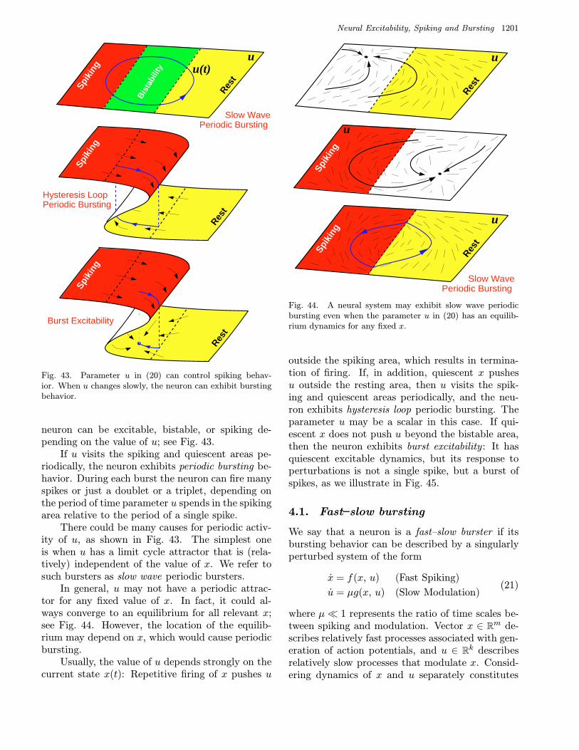
Neural Excitability, Spiking and Bursting 1201
Spik
ing
Rest
Spik
ing
Rest
Bis
tabi
lity
Sp
ikin
g
Rest
Slow WavePeriodic Bursting
Hysteresis LoopPeriodic Bursting
Burst Excitability
uu(t)
Fig. 43. Parameter u in (20) can control spiking behav-ior. When u changes slowly, the neuron can exhibit burstingbehavior.
neuron can be excitable, bistable, or spiking de-pending on the value of u; see Fig. 43.
If u visits the spiking and quiescent areas pe-riodically, the neuron exhibits periodic bursting be-havior. During each burst the neuron can fire manyspikes or just a doublet or a triplet, depending onthe period of time parameter u spends in the spikingarea relative to the period of a single spike.
There could be many causes for periodic activ-ity of u, as shown in Fig. 43. The simplest oneis when u has a limit cycle attractor that is (rela-tively) independent of the value of x. We refer tosuch bursters as slow wave periodic bursters.
In general, u may not have a periodic attrac-tor for any fixed value of x. In fact, it could al-ways converge to an equilibrium for all relevant x;see Fig. 44. However, the location of the equilib-rium may depend on x, which would cause periodicbursting.
Usually, the value of u depends strongly on thecurrent state x(t): Repetitive firing of x pushes u
Rest
u
Spik
ing
u
Spik
ing
Rest
Slow WavePeriodic Bursting
u
Fig. 44. A neural system may exhibit slow wave periodicbursting even when the parameter u in (20) has an equilib-rium dynamics for any fixed x.
outside the spiking area, which results in termina-tion of firing. If, in addition, quiescent x pushesu outside the resting area, then u visits the spik-ing and quiescent areas periodically, and the neu-ron exhibits hysteresis loop periodic bursting. Theparameter u may be a scalar in this case. If qui-escent x does not push u beyond the bistable area,then the neuron exhibits burst excitability : It hasquiescent excitable dynamics, but its response toperturbations is not a single spike, but a burst ofspikes, as we illustrate in Fig. 45.
4.1. Fast slow bursting
We say that a neuron is a fast–slow burster if itsbursting behavior can be described by a singularlyperturbed system of the form
x = f(x, u) (Fast Spiking)
u = µg(x, u) (Slow Modulation)(21)
where µ 1 represents the ratio of time scales be-tween spiking and modulation. Vector x ∈ Rm de-scribes relatively fast processes associated with gen-eration of action potentials, and u ∈ Rk describesrelatively slow processes that modulate x. Consid-ering dynamics of x and u separately constitutes

1202 E. M. Izhikevich
Perturbation
Fig. 45. Burst excitability in the Morris–Lecar model withan additional slow subsystem; see bottom of Fig. 43.
the method of dissection of neural bursting [Rinzel& Lee, 1987], or of quasistatic state approximation[Hoppensteadt, 1993].
We say that the burster is “m + k” when thefast subsystem is m-dimensional and the slow sub-system is k-dimensional. In this paper we providemany examples of “2 + 1” and “2 + 2” bursters.
4.1.1. Classical singular perturbation theory
Asymptotic theory of singularly perturbed dynam-ical systems is well-developed [Hoppensteadt, 1993;Mishchenko et al., 1994] and one would expect tofind methods to analyze fast–slow bursters of theform (21). However, the basic assumption of thetheory that the fast subsystem has only equilibriumdynamics, is violated when the neuron starts to fireperiodically. Thus, the entire bulk of theory is help-less in studying fast–slow bursting. (An exception isthe Pontryagin’s problem, which is related to “foldcycle/fold cycle” bursting; see Sec. 7 in [Mishchenkoet al., 1994]).
4.1.2. Averaging
One can try to use averaging to get some insightinto the behavior of the system (21). This approachwas used successfully, e.g. by Rinzel and Lee [1986],Pernarowski et al. [1992], Smolen et al. [1993] andBaer et al. [1995].
Let x(t) = x(t, u) be a solution of the fast sub-system when u = const. Using it in the slow sub-system results in
u = µg(x(t, u), u) ,
which can be reduced to
w = µg(w) (22)
by a near-identity change of variables w = u+o(µ).Here
g(w) = limT→∞
1
T
∫ T
0g(x(t, w), w)dt
is the average of g. Unfortunately, many problemsmay arise when u passes slowly bifurcation values.For example, the period of x(t, u) may go to infin-ity, as happens in Class 1 systems, or transients maytake as long as 1/µ units of time, or the averagedsystem (22) is not Lipchitz. In all these cases thestraightforward averaging discussed above fails. Weprovide an example when we discuss “Hopf/Hopf”hysteresis loop bursting.
4.1.3. Equivalent voltage
If a neural model exhibits bistable behavior, thenthe function g in (22) is not single-valued, but it haslayers (sheets) similar to those depicted in Fig. 43.This is the result of the averaging that removescompletely the fast dynamics. To study possiblehysteresis behavior we need to retain at least one“fast” variable. This is always possible in the fol-lowing important class of fast–slow bursters
x = f(x, u)
u = µg(h(x), u)(23)
where h : Rm → R is an arbitrary function, e.g. themembrane voltage at state x. Notice that the imageof h is a scalar.
If the slow variable is a scalar too, then for anyvalue of u there is a (possibly nonunique) value ofanother scalar, v, such that g(v, u) = g(u), whereg(u) is the averaged function defined above. Werefer to v as being the equivalent voltage [Bertramet al., 1995]. It allows to reduce (23) to the two-dimensional system of the form
v = s(v, u)
u = µg(v, u)(24)
where g is exactly the same as in (21), ands : R2 → R is some function that can be foundnumerically. Its set of zeroes often has the N -shapedepicted in Fig. 46. If (23) describes a hysteresisloop periodic burster, then system (24) is a relax-ation oscillator. Thus, most of the results regard-ing synchronization of coupled relaxation oscillatorscan be applied to coupled bursters.
4.2. Classification
Below we provide a classification scheme for peri-odic fast–slow bursting. Any such bursting involves

Neural Excitability, Spiking and Bursting 1203
u
v
s(v,u)=0
Fig. 46. The set of zeroes of function s in (24) often has anN-shape.
at least two bifurcations (see Fig. 2):
• Bifurcation of the quiescent state leading torepetitive spiking.• Bifurcation of the repetitive spiking leading to the
quiescent state.
There could also be other bifurcations, which do notswitch between the rest and spiking states. Sincethere are 12 relevant codimension 1 bifurcations ofthe quiescent state and 10 relevant codimension 1bifurcations of the spiking state, there are 120 dif-ferent types of codimension 1 bursters; see Table 4.
We refer to a burster as being planar when thefast subsystem is two-dimensional, i.e. the burster is“2 +k”. This imposes severe restriction on possiblebifurcations. In particular, there are only 24 varioustypes of planar codimension 1 fast–slow bursters,which are summarized in Table 3. We emphasizeplanar bursters because they have a greater chanceto be encountered in computer simulations.
Various bursters can be combined into groupsdepending on the nature of quiescent and spikingstate at the bifurcations. If the quiescent stateis a stable equilibrium and the spiking state is alimit cycle attractor, then we say that the burster ispoint-cycle. A cycle–cycle burster occurs when thequiescent state is a small amplitude, “subthresh-old” limit cycle attractor. Similarly, point–torusand cycle–torus bursters are when the spiking stateis quasiperiodic. A point–point bursting is discussedin Sec. 4.5. It occurs when the parameter µ in (21)is not small enough. A cycle–point bursting is alsofeasible, but we do not discuss it here.
4.2.1. What is the name?
We face a challenging problem: How to label allthose bursters? We want self-explanatory names
that are easy to remember and understand. Thus,we should not number them [Bertram et al., 1995],since it would lead, e.g. to bursters of Type XXVII,Type LXIII, Type LCXVI, etc. We cannot use de-scriptions such as “elliptic”, “parabolic”, “hyper-bolic”, “triangular”, “rectangular”, etc., since theyare misleading. Instead, we base our nomenclatureon the names of the two bifurcations involved. Still,many bifurcations have multiple names. For exam-ple, a fold bifurcation is also known as saddle–node,tangent, or limit point bifurcation. Whenever pos-sible we choose the shortest name. For example,we refer to the saddle–node on invariant circle bi-furcation (also known as fold or saddle–node onlimit cycle) as just a circle bifurcation, partiallybecause it is the only codimension 1 bifurcation ofa circle flow. We refer to an Andronov–Hopf bi-furcation, also known as Poincare–Andronov–Hopf,as just Hopf when it is supercritical and subHopfwhen it is subcritical. Our results are summarizedin Table 4. For example, the famous “square-wave”(Type I) burster is a “fold/homoclinic” burster ac-cording to our classification, because the rest statedisappears via fold bifurcation and the limit cycleattractor disappears via saddle homoclinic orbit bi-furcation; see Fig. 59.
4.3. Planar point cycle bursting
In this section we give examples of planar point–cycle bursters. For this we add slow subsystemsto some well-known neural models, such as Morris–Lecar, that have sufficiently rich bifurcation struc-ture. The easiest way to get bursting is to takea two-dimensional slow subsystem having a “slowwave” (subcellular) limit cycle attractor that inter-sects the desired bifurcation curves of a fast (spik-ing) subsystem. All such bursters are “2 + 2”.This is a classical approach to obtain the “cir-cle/circle” (“parabolic”) bursting [Ermentrout &Kopell, 1986a, 1986b]. We show, however, that eachburster can be of hysteresis loop type with only oneslow variable, although finding an example of such“2 + 1” bursting is more difficult.
For the sake of convenience, we provide a list ofreferences to relevant illustrations in Table 5.
4.3.1. Slow wave bursting
Consider the four types of planar point–cycle burst-ing that are depicted in the upper left corner ofTable 4. All of them can be generated by a

Table 4. A classification of codimension 1 fast–slow bursters. See also Figs. 53 and 126.
Saddle–Node Saddle Fold Saddle Focus Focus Focus Fold Cycle onon Invariant Homoclinic Supercritical Limit Subcritical Subcritical Homoclinic Homoclinic Blue-sky Homoclinic
Bifurcations Circle Orbit Andronov–Hopf Cycle Flip Neimark–Sacker Orbit Orbit Catastrophe Torus
Fold fold/ fold/ fold/ fold/ fold/ fold/ fold/ fold/ fold/ fold/circle homoclinic Hopf fold cycle flip Sacker saddle–focus focus–focus blue-sky torus
homoclinic homoclinic
Saddle–Node circle/ circle/ circle/ circle/ circle/ circle/ circle/ circle/ circle/ circle/on Invariant circle homoclinic Hopf fold cycle flip Sacker saddle–focus focus–focus blue-sky torusCircle homoclinic homoclinic
Supercritical Hopf/ Hopf/ Hopf/ Hopf/ Hopf/ Hopf/ Hopf/ Hopf/ Hopf/ Hopf/Andronov– circle homoclinic Hopf fold cycle flip Sacker saddle–focus focus–focus blue-sky torusHopf homoclinic homoclinic
Subcritical subHopf/ subHopf/ subHopf/ subHopf/ subHopf/ subHopf/ subHopf/ subHopf/ subHopf/ subHopf/Andronov– circle homoclinic Hopf fold cycle flip Sacker saddle–focus focus–focus blue-sky torusHopf homoclinic homoclinic
Fold fold cycle/ fold cycle/ fold cycle/ fold cycle/ fold cycle/ fold cycle/ fold cycle/ fold cycle/ fold cycle/ fold cycle/Limit circle homoclinic Hopf fold cycle flip Sacker saddle–focus focus–focus blue-sky torusCycle homoclinic homoclinic
Saddle homoclinic/ homoclinic/ homoclinic/ homoclinic/ homoclinic/ homoclinic/ homoclinic/ homoclinic/ homoclinic/ homoclinic/Homoclinic circle homoclinic Hopf fold cycle flip Sacker saddle–focus focus–focus blue-sky torusOrbit homoclinic homoclinic
1204

Subcritical flip/ flip/ flip/ flip/ flip/ flip/ flip/ flip/ flip/ flip/Flip circle homoclinic Hopf fold cycle flip Sacker saddle–focus focus–focus blue-sky torus
homoclinic homoclinic
Subcritical Sacker/ Sacker/ Sacker/ Sacker/ Sacker/ Sacker/ Sacker/ Sacker/ Sacker/ Sacker/Neimark– circle homoclinic Hopf fold cycle flip Sacker saddle–focus focus–focus blue-sky torusSacker homoclinic homoclinic
Saddle Focus saddle–focus saddle–focus saddle–focus saddle–focus saddle–focus saddle–focus saddle–focus saddle–focus saddle–focus saddle–focus
Homoclinic homoclinic/ homoclinic/ homoclinic/ homoclinic/ homoclinic/ homoclinic/ homoclinic/ homoclinic/ homoclinic/ homoclinic/Orbit circle homoclinic Hopf fold cycle flip Sacker saddle–focus focus–focus blue-sky torus
homoclinic homoclinic
Focus Focus focus–focus focus–focus focus–focus focus–focus focus–focus focus–focus focus–focus focus–focus focus–focus homoclinic/
Homoclinic homoclinic/ homoclinic/ homoclinic/ homoclinic/ homoclinic/ homoclinic/ homoclinic/ homoclinic/ homoclinic/ torusOrbit circle homoclinic Hopf fold cycle flip Sacker saddle–focus focus–focus blue-sky
homoclinic homoclinic
Blue Sky blue-sky/ blue-sky/ blue-sky/ blue-sky/ blue-sky/ blue-sky/ blue-sky/ blue-sky/ blue-sky/ blue-sky/Catastrophe circle homoclinic Hopf fold cycle flip Sacker saddle–focus focus–focus blue-sky torus
homoclinic homoclinic
Fold Cycle on torus/ torus/ torus/ torus/ torus/ torus/ torus/ torus/ torus/ torus/Homoclinic circle homoclinic Hopf fold cycle flip Sacker saddle–focus focus–focus blue-sky torusTorus homoclinic homoclinic
Planar Point-TorusPoint-Cycle Cycle-Cycle Cycle-Torus
1205

1206 E. M. Izhikevich
Table 5. A list of figure numbers.
Saddle–Node Saddle Foldon Invariant Homoclinic Supercritical Limit
Bifurcations Circle Orbit Andronov–Hopf Cycle
Fold 47, 61, 87 47, 59, 60, 86 63 68, 87
Saddle-Node 47, 49, 47, 62, 87 67 64, 65, 66
on Invariant 52, 56, 57,
Circle 58, 87
Supercritical 72 71 48, 83, 48, 75
Andronov–Hopf 84, 85
Subcritical 73, 74, 87 69, 70, 87 48, 76, 77 48, 78,
Andronov–Hopf 80, 82
Fold Limit 98 97 99 93, 94, 96
Cycle
Saddle 92 88, 89 90 92
HomoclinicOrbit
Fold/Circle("triangular")
Circle/Circle("parabolic")
Fold/Homoclinic("square-wave")
Circle/Homoclinic
circ
lefo
ld
homoclinic
Fig. 47. A neural system near saddle–node separatrix loopbifurcation (see Fig. 22) can exhibit four different types offast–slow bursting.
system near a saddle–node separatrix loop bifur-
cation that we discussed in Sec. 2.3. Indeed, thetwo-dimensional vector of bifurcation parameters
can slowly cross the bifurcation curves depicted inFig. 22. The type of bursting would depend on the
location of the slow limit cycle; see Fig. 47.
Similarly, a system near a Bautin bifurca-tion can exhibit four types of bursting when the
bifurcation parameters a and b in topological nor-mal form (12) change slowly; see Fig. 48.
The figures illustrate an important issue: Manybursters, such as “circle/homoclinic”, “fold/circle”,“Hopf/fold cycle”, and “subHopf/Hopf”, may in-volve more than two bifurcations. For example, the“circle/homoclinic” bursting from Fig. 47 exhibitsa fold bifurcation during the spiking stage. The bi-furcation does not turn the spiking off, but it givesbirth to a stable rest state and a saddle, which willparticipate in the saddle homoclinic orbit bifurca-tion that turns the spiking off.
Since there can be many other bifurcations ofthe quiescent and spiking state besides those re-sponsible for onset and termination of the spikingphase, the latter two do not define the type of burst-ing uniquely, but rather specify a large class, whichmay have subtypes.
4.3.2. Hysteresis loop bursting
The vector of bifurcation parameters in Figs. 47and 48 has a slow limit cycle attractor. There-fore all those bursters are of the slow wave type.One can easily make the “fold/homoclinic” and the“subHopf/fold cycle” bursters to be of hysteresisloop type by taking advantage of the bistabilityof attractors.
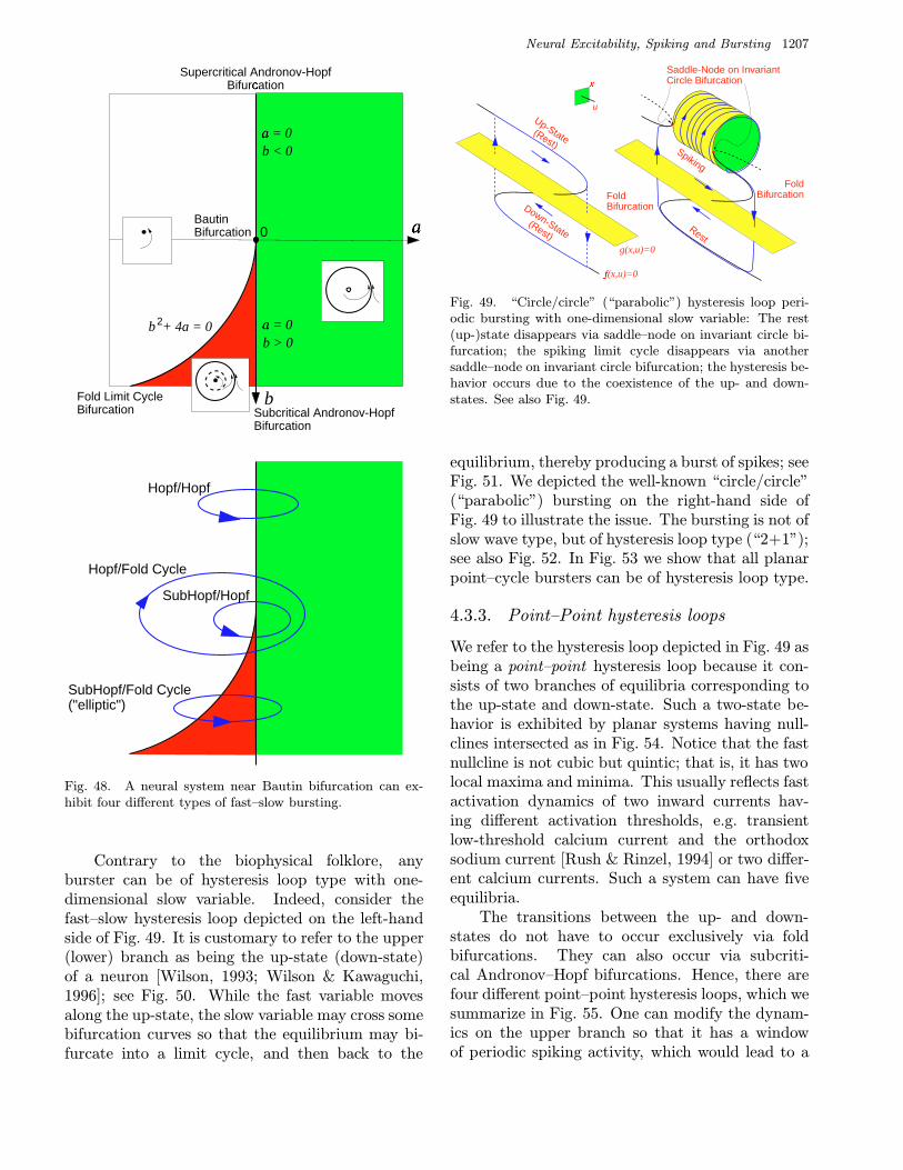
Neural Excitability, Spiking and Bursting 1207
Fold Limit CycleBifurcation Subcritical Andronov-Hopf
Bifurcation
Supercritical Andronov-HopfBifurcation
BautinBifurcation
b + 4a = 02
b < 0
0
a = 0
a
b
b > 0a = 0
SubHopf/Fold Cycle("elliptic")
Hopf/Fold Cycle
SubHopf/Hopf
Hopf/Hopf
Fig. 48. A neural system near Bautin bifurcation can ex-hibit four different types of fast–slow bursting.
Contrary to the biophysical folklore, anyburster can be of hysteresis loop type with one-dimensional slow variable. Indeed, consider thefast–slow hysteresis loop depicted on the left-handside of Fig. 49. It is customary to refer to the upper(lower) branch as being the up-state (down-state)of a neuron [Wilson, 1993; Wilson & Kawaguchi,1996]; see Fig. 50. While the fast variable movesalong the up-state, the slow variable may cross somebifurcation curves so that the equilibrium may bi-furcate into a limit cycle, and then back to the
Rest
Spiking
x
u
Saddle-Node on InvariantCircle Bifurcation
FoldBifurcation
FoldBifurcation
Up-State(Rest)
Down-State(Rest)
f(x,u)=0
g(x,u)=0
Fig. 49. “Circle/circle” (“parabolic”) hysteresis loop peri-odic bursting with one-dimensional slow variable: The rest(up-)state disappears via saddle–node on invariant circle bi-furcation; the spiking limit cycle disappears via anothersaddle–node on invariant circle bifurcation; the hysteresis be-havior occurs due to the coexistence of the up- and down-states. See also Fig. 49.
equilibrium, thereby producing a burst of spikes; seeFig. 51. We depicted the well-known “circle/circle”(“parabolic”) bursting on the right-hand side ofFig. 49 to illustrate the issue. The bursting is not ofslow wave type, but of hysteresis loop type (“2+1”);see also Fig. 52. In Fig. 53 we show that all planarpoint–cycle bursters can be of hysteresis loop type.
4.3.3. Point–Point hysteresis loops
We refer to the hysteresis loop depicted in Fig. 49 asbeing a point–point hysteresis loop because it con-sists of two branches of equilibria corresponding tothe up-state and down-state. Such a two-state be-havior is exhibited by planar systems having null-clines intersected as in Fig. 54. Notice that the fastnullcline is not cubic but quintic; that is, it has twolocal maxima and minima. This usually reflects fastactivation dynamics of two inward currents hav-ing different activation thresholds, e.g. transientlow-threshold calcium current and the orthodoxsodium current [Rush & Rinzel, 1994] or two differ-ent calcium currents. Such a system can have fiveequilibria.
The transitions between the up- and down-states do not have to occur exclusively via foldbifurcations. They can also occur via subcriti-cal Andronov–Hopf bifurcations. Hence, there arefour different point–point hysteresis loops, which wesummarize in Fig. 55. One can modify the dynam-ics on the upper branch so that it has a windowof periodic spiking activity, which would lead to a

1208 E. M. Izhikevich
10 mV
500 ms
-49 mV
-63 mV
Up-State
Down-State
Fig. 50. Intracellular recordings of spontaneous activity of neostriatal spiny cells reveal two-state behavior. Notice that onlythe up-state is excitable. (Courtesy of Charles Wilson, University of Tennessee.)
Rest
Point-PointHysteresisLoop
Hysteresis LoopPeriodic Bursting
Rest
Up-state
Down-state
Spiking
Rest
Rest
Up-state
Down-state
Spiking
Fig. 51. Modification of dynamics on the upper branch ofthe point–point hysteresis loop: The slow variable crossesbifurcation curves, creates a window of periodic spiking ac-tivity, and results in bursting behavior.
hysteresis loop bursting, as in Fig. 51. For exam-ple, one can put two “circle” bifurcations on theupper branch of any of the hysteresis loops, as wedo in Fig. 56, and get four different subtypes ofthe “circle/circle” bursting. Similarly, one can have
four subtypes of “circle/Hopf”, “Hopf/circle”, and“Hopf/Hopf” hysteresis loop bursters.
A remarkable fact is that the point–point hys-teresis loops themselves can exhibit bursting behav-ior despite the fact that there are no stable limit cy-cles. This happens when the small parameter µ in(21) is not small enough, as we discuss in Sec. 4.5.
Considering point–point hysteresis loops raisesthe following issue: The spiking state during the ac-tive phase of bursting might be irrelevant to whatthe cell is doing. For example, the pancreatic β-cells secrete insulin while they are in the up-stateregardless whether their membranes produce spikesor not. Similarly, neurons without axons, such asgranule cells in the olfactory bulb, or with shortaxons, such as many interneurons, may not needspikes to activate synaptic transmission. A meretransition to the up-state may be enough to trig-ger release of neurotransmitter. Even if such cellsexhibit bursting dynamics, their essential neuro-computational features might depend only on thetype of the hysteresis loop. In contrast, if a burstingneuron has a long axon, then it might need prop-agating spikes to trigger synaptic transmission indistant synapses. In this case it is important tounderstand the mechanism of initiation and termi-nation of repetitive spiking during the burst.
4.3.4. “Circle/circle” (“parabolic”) bursting
The transition from quiescent state to repetitivespiking and back occurs via a saddle-node on in-variant circle bifurcation; see Fig. 47. Since thefrequency of emerging and terminating spiking

Rest
Spiking
Saddle-Node on InvariantCircle Bifurcation
FoldBifurcation
FoldBifurcation
x
u
"Circle/Circle" Bursting
0 200 400 600 800 1000 1200 1400 1600 1800-0.7
-0.6
-0.5
-0.4
-0.3
-0.2
-0.1
0
0.1
0.2
0.3
Saddle-Node on
Invariant Circle
Fold
Saddle-Node on
Invariant Circle
Fold
V(t)
Fig. 52. “Circle/circle” (“parabolic”) bursting via “fold/fold” hysteresis loop: The transition from quiescent state to repetitivespiking and back occurs via a saddle–node on invariant circle bifurcation. The transitions between the down-state (lowerbranch) and the up-state (upper branch) occur via fold bifurcations. Shown are simulations of the Morris–Lecar system withtwo additional low-threshold currents: Inward current as in Fig. 62 and an outward current IR(V, u) = 0.2(1 + tanh(V +0.3)/0.1)u4(Ek − V ). The other parameters and variables are as in Fig. 62 except I = −0.067 and µ = 0.0025.
1209

1210 E. M. Izhikevich
"Fold/Circle" Bursting
Saddle-Node onInvariant Circle
Saddle
Homoclinic OrbitSupercritical
Andronov-Hopf Fold Limit Cycle
"Fold/Homoclinic" Bursting "Fold/Hopf" Bursting "Fold/Fold Cycle" Bursting
"Circle/Circle" Bursting "Circle/Homoclinic" Bursting "Circle/Hopf" Bursting "Circle/Fold Cycle" Bursting
"Hopf/Circle" Bursting "Hopf/Homoclinic" Bursting "Hopf/Hopf" Bursting "Hopf/Fold Cycle" Bursting
"SubHopf/Circle" Bursting "SubHopf/Homoclinic"Bursting
"SubHopf/Hopf" Bursting "SubHopf/Fold Cycle"Bursting
Fol
d
Sad
dle-
Nod
e on
Inva
riant
Circ
le
Sup
ercr
itica
l
And
rono
v-H
opf
Sub
criti
cal
And
rono
v-H
opf
Bifurcation of Spiking StateB
ifu
rcat
ion
of
Qu
iesc
ent
Sta
te
Fig. 53. Examples of planar point–cycle fast–slow codimension 1 bursters of hysteresis loop type.

Neural Excitability, Spiking and Bursting 1211
Up-State
Down-State
v
w
v'=0
w'=0
Up-StateDown-State v
w
v'=0
w'=0
Fig. 54. Possible intersections of nullclines in planar system v′ = f(v, w), w′ = µg(v, w) that would result in the two-statebehavior depicted in Fig. 50 with only the up-state being excitable (notice the blue periodic pseudo-orbits). Here v and w arethe voltage and recovery variables, respectively.
FoldBifurcation
FoldBifurcation
Saddle HomoclinicOrbit Bifurcation
FoldBifurcation
SubcriticalAndrono-HopfBifurcation
FoldBifurcation Saddle Homoclinic
Orbit Bifurcation
SubcriticalAndrono-Hopf
Bifurcation
SubcriticalAndrono-Hopf
Bifurcation
SubcriticalAndrono-HopfBifurcation
Saddle
HomoclinicOrbit
Bifurcations
"Fold/Fold"
Hysteresis Loop"Fold/SubHopf"Hysteresis Loop
"SubHopf/Fold"Hysteresis Loop
"SubHopf/SubHopf"
Hysteresis Loop
Fig. 55. Classification of point–point hysteresis loops.

1212 E. M. Izhikevich
SubcriticalAndronov-HopfBifurcation
Saddle HomoclinicOrbit Bifurcation
SubcriticalAndronov-Hopf
Bifurcation
SubcriticalAndronov-Hopf
Bifurcation
SubcriticalAndronov-HopfBifurcation
SaddleHomoclinic
OrbitBifurcations
"Circle/Circle" Burstingvia "Fold/Fold"
Hysteresis Loop
"Circle/Circle" Bursting via "Fold/SubHopf"
Hysteresis Loop
"Circle/Circle" Burstingvia "SubHopf/Fold"
Hysteresis Loop
"Circle/Circle" Burstingvia "SubHopf/SubHopf"
Hysteresis Loop
Rest
Spiking
Saddle-Node on InvariantCircle Bifurcation
FoldBifurcation
Rest
Spiking
Saddle-Node on InvariantCircle Bifurcation
FoldBifurcation
Rest
Spiking
Saddle-Node on InvariantCircle Bifurcation
Spiking
Saddle-Node on InvariantCircle Bifurcation
FoldBifurcationFold
Bifurcation
Fig. 56. Subtypes of the “circle/circle” hysteresis loop bursting. See Fig. 55 for reference.

Neural Excitability, Spiking and Bursting 1213
Spike Spike
Inte
rspi
ke P
erio
d
Inte
rspi
ke F
requ
ency
Fig. 57. The interspike period in the “circle/circle” burstingresembles a parabola, which motivates the name “parabolicbursting”.
behaves as√λ, where λ is the distance to the bifur-
cation, the interspike period “looks” like a parabola(see Fig. 57), which motivates the name “parabolicbursting”. Such a bursting is exhibited by theR15 cells in the abdominal ganglion of the molluskAplysia and it has been studied by many scien-tists, including Plant [1981], Rinzel and Lee [1987],Ermentrout and Kopell [1986a, 1986b], Canavieret al. [1991], Bertram [1993], Baer et al. [1995],Bertram et al. [1995], Soto-Trevino et al. [1996], andButera et al. [1996, 1997], Hoppensteadt [1997], andTaylor and Holmes [1998].
Under fairly general conditions, any slow wave“circle/circle” burster can be transformed to theErmentrout–Kopell canonical model [Ermentrout &Kopell, 1986a, 1986b; Hoppensteadt & Izhikevich,1997]
ϑ = 1− cos ϑ+ (1 + cos ϑ)r(ψ)
ψ = ω
where r : S1 → R is some function that depends onparticulars of the burster, e.g. r(ψ) = cos ψ. Whenr(ψ) < 0, the cell is quiescent; When r(ψ) > 0,it fires periodically; see Fig. 58. As was shown bySoto-Trevino et al. [1995], the slow subsystem doesnot need a limit cycle attractor to exhibit periodicbursting; it might be just excitable; see detailed dis-cussion in Sec. 8.2.3 by Hoppensteadt and Izhike-vich [1997].
As we discussed above, there can be at leastfour subtypes of hysteresis loop “circle/circle”bursting having one-dimensional slow variable(i.e. “2 + 1” bursting); see Figs. 52 and 56.
Saddle-Node onInvariant CircleBifurcation
θ
ψ
Saddle-Node onInvariant Circle
BifurcationSpiking
Rest
Fig. 58. “Circle/circle” (“parabolic”) slow wave bursting.Variables θ, ψ ∈ S1.
4.3.5. “Fold/homoclinic” (“square-wave”)bursting
The rest state disappears via fold bifurcation,and the periodic spiking disappears via saddle-homoclinic orbit bifurcation; see Fig. 47. Sincethere is a coexistence of attractors, such burstingoccurs via “fold/homoclinic” hysteresis loop; seeFig. 59. It is often referred to as being “square-wave” bursting due to the voltage amplitude profile;see however Fig. 123.
This type of bursting is exhibited by pancre-atic β-cells; see [Chay & Keizer, 1983; Pernarowskiet al., 1992] and references therein. It is ubiquitousin many systems [Alexander & Cai, 1991] includingHindmarsh and Rose [1984] model [Wang, 1993],Chay–Cook [Bertram et al., 1995] model, and thereduced Morris–Lecar model
V = I − gl(V −El)− gkw(V −Ek)
− gCam∞(V )(V −ECa)
w = λ(V )(w∞(V )− w)
(25)
where
m∞(V ) =1
2
(1 + tanh
V − V1
V2
)
w∞(V ) =1
2
(1 + tanh
V − V3
V4
)
λ(V ) =1
3cosh
V − V3
2V4.
We assume I(u) = −u and use a linear slowsubsystem
u = µ(0.2 + V ) (26)
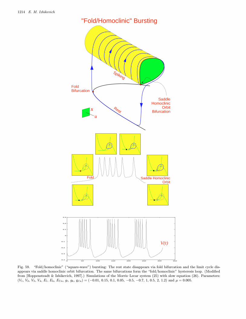
1214 E. M. Izhikevich
0 50 100 150 200 250 300 3500.4
0.3
0.2
0.1
0
0.1
0.2
0.3
V(t)
Fold Saddle HomoclinicOrbit
"Fold/Homoclinic" Bursting
x
u
FoldBifurcation
Rest
Spiking
SaddleHomoclinic
OrbitBifurcation
Fig. 59. “Fold/homoclinic” (“square-wave”) bursting: The rest state disappears via fold bifurcation and the limit cycle dis-appears via saddle homoclinic orbit bifurcation. The same bifurcations form the “fold/homoclinic” hysteresis loop. (Modifiedfrom [Hoppensteadt & Izhikevich, 1997].) Simulations of the Morris–Lecar system (25) with slow equation (26). Parameters:(V1, V2, V3, V4, El, Ek, ECa, gl, gk, gCa) = (−0.01, 0.15, 0.1, 0.05, −0.5, −0.7, 1, 0.5, 2, 1.2) and µ = 0.005.
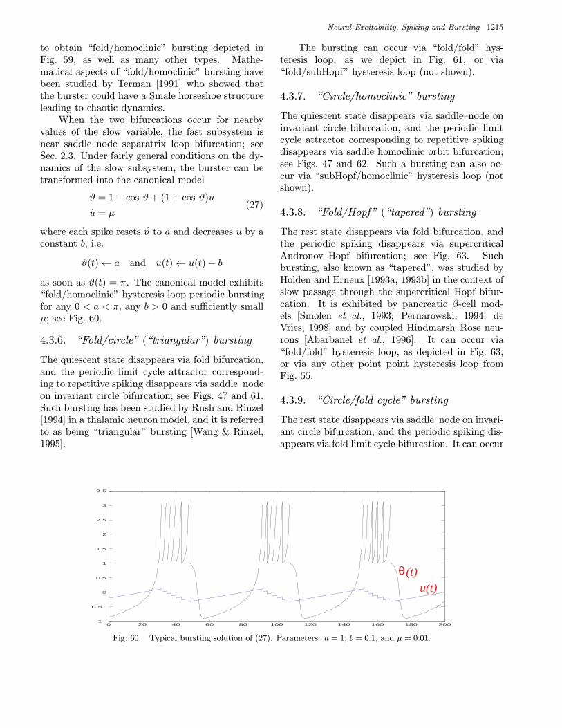
Neural Excitability, Spiking and Bursting 1215
to obtain “fold/homoclinic” bursting depicted inFig. 59, as well as many other types. Mathe-matical aspects of “fold/homoclinic” bursting havebeen studied by Terman [1991] who showed thatthe burster could have a Smale horseshoe structureleading to chaotic dynamics.
When the two bifurcations occur for nearbyvalues of the slow variable, the fast subsystem isnear saddle–node separatrix loop bifurcation; seeSec. 2.3. Under fairly general conditions on the dy-namics of the slow subsystem, the burster can betransformed into the canonical model
ϑ = 1− cos ϑ+ (1 + cos ϑ)u
u = µ(27)
where each spike resets ϑ to a and decreases u by aconstant b; i.e.
ϑ(t)← a and u(t)← u(t)− b
as soon as ϑ(t) = π. The canonical model exhibits“fold/homoclinic” hysteresis loop periodic burstingfor any 0 < a < π, any b > 0 and sufficiently smallµ; see Fig. 60.
4.3.6. “Fold/circle” (“triangular”) bursting
The quiescent state disappears via fold bifurcation,and the periodic limit cycle attractor correspond-ing to repetitive spiking disappears via saddle–nodeon invariant circle bifurcation; see Figs. 47 and 61.Such bursting has been studied by Rush and Rinzel[1994] in a thalamic neuron model, and it is referredto as being “triangular” bursting [Wang & Rinzel,1995].
The bursting can occur via “fold/fold” hys-teresis loop, as we depict in Fig. 61, or via“fold/subHopf” hysteresis loop (not shown).
4.3.7. “Circle/homoclinic” bursting
The quiescent state disappears via saddle–node oninvariant circle bifurcation, and the periodic limitcycle attractor corresponding to repetitive spikingdisappears via saddle homoclinic orbit bifurcation;see Figs. 47 and 62. Such a bursting can also oc-cur via “subHopf/homoclinic” hysteresis loop (notshown).
4.3.8. “Fold/Hopf” (“tapered”) bursting
The rest state disappears via fold bifurcation, andthe periodic spiking disappears via supercriticalAndronov–Hopf bifurcation; see Fig. 63. Suchbursting, also known as “tapered”, was studied byHolden and Erneux [1993a, 1993b] in the context ofslow passage through the supercritical Hopf bifur-cation. It is exhibited by pancreatic β-cell mod-els [Smolen et al., 1993; Pernarowski, 1994; deVries, 1998] and by coupled Hindmarsh–Rose neu-rons [Abarbanel et al., 1996]. It can occur via“fold/fold” hysteresis loop, as depicted in Fig. 63,or via any other point–point hysteresis loop fromFig. 55.
4.3.9. “Circle/fold cycle” bursting
The rest state disappears via saddle–node on invari-ant circle bifurcation, and the periodic spiking dis-appears via fold limit cycle bifurcation. It can occur
0 20 40 60 80 100 120 140 160 180 2001
0.5
0
0.5
1
1.5
2
2.5
3
3.5
θ(t)u(t)
Fig. 60. Typical bursting solution of (27). Parameters: a = 1, b = 0.1, and µ = 0.01.
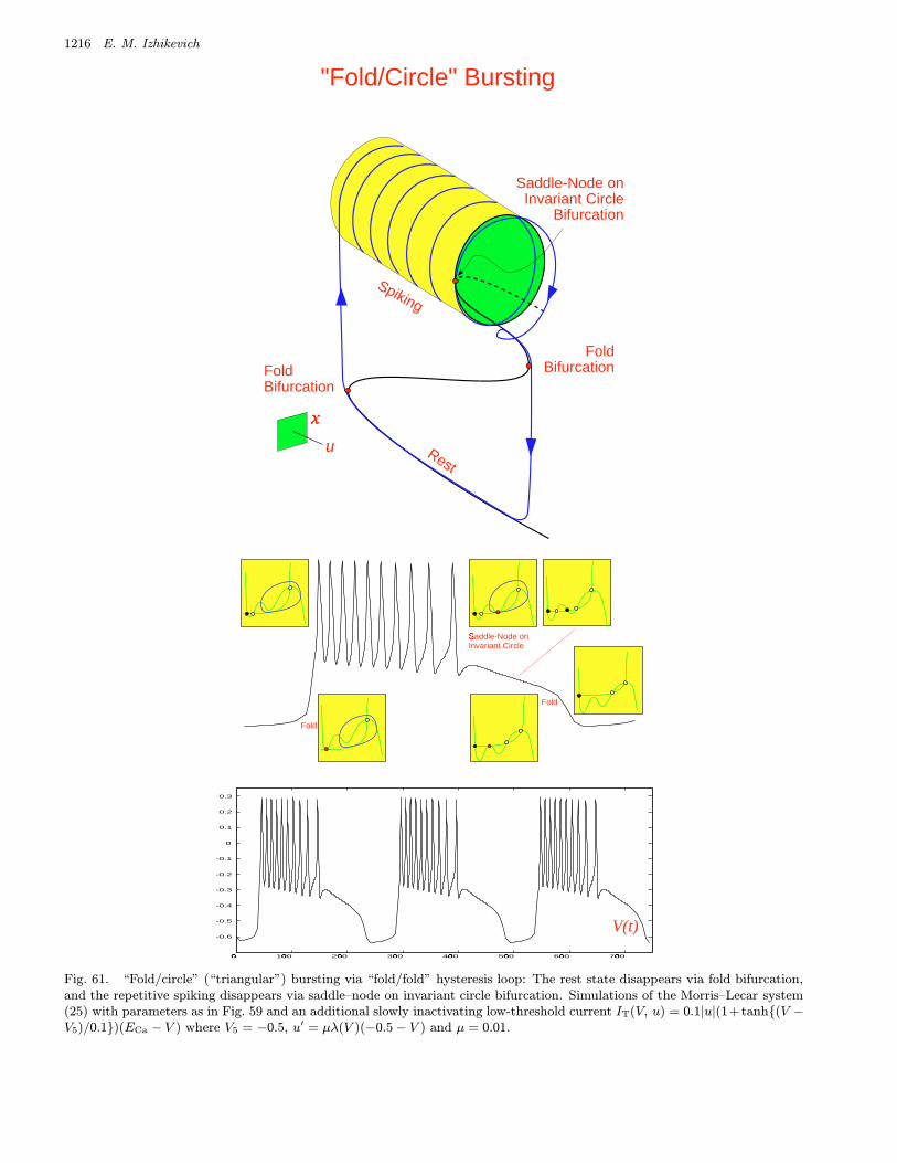
1216 E. M. Izhikevich
x
u
Saddle-Node onInvariant Circle
Bifurcation
FoldBifurcationFold
Bifurcation
Rest
Spiking
"Fold/Circle" Bursting
0 100 200 300 400 500 600 700
-0.6
-0.5
-0.4
-0.3
-0.2
-0.1
0
0.1
0.2
0.3
V(t)
Saddle-Node on
Invariant Circle
Fold
Fold
Fig. 61. “Fold/circle” (“triangular”) bursting via “fold/fold” hysteresis loop: The rest state disappears via fold bifurcation,and the repetitive spiking disappears via saddle–node on invariant circle bifurcation. Simulations of the Morris–Lecar system(25) with parameters as in Fig. 59 and an additional slowly inactivating low-threshold current IT(V, u) = 0.1|u|(1+tanh(V −V5)/0.1)(ECa − V ) where V5 = −0.5, u′ = µλ(V )(−0.5− V ) and µ = 0.01.

Neural Excitability, Spiking and Bursting 1217
x
u
Saddle-Node onInvariant CircleBifurcation
FoldBifurcation
Rest
Spiking
SaddleHomoclinic
OrbitBifurcation
SaddleHomoclinic Orbit
"Circle/Homoclinic" Bursting
0 100 200 300 400 500 600 700
-0.6
-0.5
-0.4
-0.3
-0.2
-0.1
0
0.1
0.2
0.3
V(t)
Saddle-Node on
Invariant Circle
Fold
Fig. 62. “Circle/homoclinic” bursting via “fold/homoclinic” hysteresis loop: The rest state disappears via saddle–node oninvariant circle bifurcation, and the spiking state disappears via saddle homoclinic orbit bifurcation. Simulations of theMorris–Lecar system with additional current as in Fig. 61 except that V5(u) = −0.8− 0.5u.

1218 E. M. Izhikevich
x
u
FoldBifurcation
FoldBifurcation
Rest
Spiking
SupercriticalAndronov-Hopf
Bifurcation
0 100 200 300 400 500 600 7002
1.5
1
0.5
0
0.5
1
1.5
2
v(t)
Fold
SupercriticalAndronov-Hopf
Fold
"Fold/Hopf" Bursting
Fig. 63. “Fold/Hopf” (”tapered”) bursting via “fold/fold” hysteresis loop: The rest state disappears via fold bifurcation,and the repetitive spiking disappears via supercritical Andronov–Hopf bifurcation. Simulations of (15) with slow subsystemc = µv. Parameters: (a, b, d, ε, µ) = (−1.55, 2.5, 0.1, 0.5, 0.01).
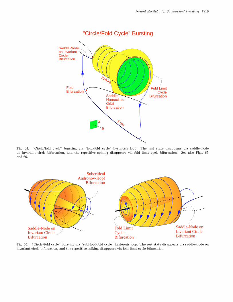
Neural Excitability, Spiking and Bursting 1219
Saddle-Nodeon InvariantCircleBifurcation
x
u
FoldBifurcation
Rest
Spiking
Fold LimitCycle
Bifurcation
"Circle/Fold Cycle" Bursting
SaddleHomoclinicOrbitBifurcation
Fig. 64. “Circle/fold cycle” bursting via “fold/fold cycle” hysteresis loop: The rest state disappears via saddle–nodeon invariant circle bifurcation, and the repetitive spiking disappears via fold limit cycle bifurcation. See also Figs. 65and 66.
SubcriticalAndronov-Hopf
Bifurcation
Saddle-Node onInvariant CircleBifurcation
Fold LimitCycleBifurcation
Saddle-Node onInvariant CircleBifurcation
Fig. 65. “Circle/fold cycle” bursting via “subHopf/fold cycle” hysteresis loop: The rest state disappears via saddle–node oninvariant circle bifurcation, and the repetitive spiking disappears via fold limit cycle bifurcation.

1220 E. M. Izhikevich
via “fold/fold cycle hysteresis loop, as depicted inFig. 64, or via “subHopf/fold cycle” hysteresis loopas depicted in Figs. 65 and 66.
4.3.10. “Circle/Hopf” bursting
The quiescent state disappears via saddle–node bi-furcation on invariant circle, and the periodic limitcycle attractor corresponding to repetitive spikingshrinks to a point via supercritical Andronov–Hopfbifurcation. It can occur via “fold/fold” hystere-sis loop as we depict in Fig. 67, or via any otherpoint–point hysteresis loop from Fig. 55.
4.3.11. “Fold/Fold cycle” bursting
The quiescent state disappears via fold bifurcation,and the periodic limit cycle attractor correspond-ing to repetitive spiking disappears via fold limitcycle bifurcation; see Fig. 68. Such a bursting wasfirst discovered in Chay–Cook model by Bertram
et al. [1995], who referred to it as being a Type IVbursting.
4.3.12. “SubHopf/homoclinic” bursting
The quiescent state disappears via subcriticalAndronov–Hopf bifurcation, and the periodic limitcycle attractor corresponding to repetitive spik-ing disappears via saddle homoclinic orbit bi-furcation. The bursting can occur via “fold/homoclinic” hysteresis loop, see Fig. 69, or via“subHopf/homoclinic” hysteresis loop as depictedin Fig. 70.
4.3.13. “Hopf/homoclinic” bursting
The quiescent state disappears via supercriticalAndronov–Hopf bifurcation, and the periodic limitcycle attractor corresponding to repetitive spik-ing disappears via saddle homoclinic orbit bifurca-tion. The bursting can occur via “fold/homoclinic”
0 100 200 300 400 500 600 700 800 900 10000.5
0.4
0.3
0.2
0.1
0
0.1
0.2
0.3
0.4
V(t)
Saddle-Nodeon InvariantCircle
Fold LimitCycle
SubcriticalAndronov-
Hopf
Fig. 66. “Circle/fold cycle” bursting via “subHopf/fold cycle” hysteresis loop (see Fig. 65) in the Morris–Lecar system (25)with slow subsystem u = µ(0.1 + V ). Parameters gCa = 1.36, V4 = 0.16, µ = 0.003, the rest as in Fig. 59.
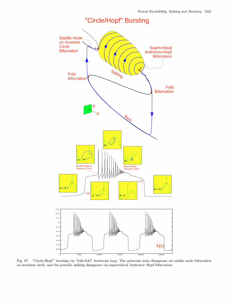
Neural Excitability, Spiking and Bursting 1221
x
u
FoldBifurcation
FoldBifurcation
Rest
Spiking
SupercriticalAndronov-Hopf
Bifurcation
Saddle-Nodeon InvariantCircleBifurcation
"Circle/Hopf" Bursting
0 500 1000 1500 2000 2500
-0.6
-0.5
-0.4
-0.3
-0.2
-0.1
0
0.1
0.2
0.3
V(t)
Saddle-Node on
Invariant Circle
Fold
Fold
Supercritical
Andronov-Hopf
Fig. 67. “Circle/Hopf” bursting via “fold/fold” hysteresis loop: The quiescent state disappears via saddle–node bifurcationon invariant circle, and the periodic spiking disappears via supercritical Andronov–Hopf bifurcation.

1222 E. M. Izhikevich
x
u
FoldBifurcation
Rest
Spiking
Fold LimitCycle
Bifurcation
Fold LimitCycle
Fold
Saddle
Homoclinic Orbit
0 50 100 150 200 250 300 350 4000
0.1
0.2
0.3
0.4
0.5
0.6
0.7
0.8
0.9
1
x(t)
"Fold/Fold Cycle" Bursting
SaddleHomoclinicOrbitBifurcation
Fig. 68. “Fold/fold cycle” (Type IV) bursting: The quiescent state disappears via fold bifurcation, and the periodic spikingdisappears via fold limit cycle bifurcation. The same bifurcations form the “fold/fold cycle” hysteresis loop. Shown aresimulations of the Wilson–Cowan [1972] model with parameters as in [Hoppensteadt & Izhikevich, 1997, Fig. 2.12], andrx(u) = −4.76 + u, ry = −9.7 + 0.3u, where u = µ(0.5− x) is a slow subsystem, µ = 0.1.

Neural Excitability, Spiking and Bursting 1223
0 500 1000 1500 20000.4
0.3
0.2
0.1
0
0.1
0.2
0.3
V(t)
Fold LimitCycle
Fold
SubcriticalAndronov-Hopf
SaddleHomoclinicOrbit
x
u
FoldBifurcation
Rest
Spiking
SaddleHomoclinic
OrbitBifurcation
Fold LimitCycleBifurcation
SubcriticalAndronov-Hopf
Bifurcation
"SubHopf/Homoclinic" Bursting
Fig. 69. “SubHopf/homoclinic” bursting via “fold/homoclinic” hysteresis loop: The quiescent state disappears via subcriticalAndronov–Hopf bifurcation, and the periodic spiking disappears via saddle homoclinic orbit bifurcation. Simulations of theMorris–Lecar model. Parameters gCa = 0.9, V4 = 0.04, V3(u) = 0.08 − u, I(u) = 0.08 − 0.03u, where u = µ(0.22 + V ) andµ = 0.003, the rest as in Fig. 59.

1224 E. M. Izhikevich
Rest
Spiking
Saddle HomoclinicOrbit Bifurcation
"SubHopf/Homoclinic" Bursting
SubcriticalAndronov-HopfBifurcation
Saddle HomoclinicOrbit Bifurcation
Fig. 70. “SubHopf/homoclinic” bursting: The quiescent state disappears via subcritical Andronov–Hopf bifurcation, and theperiodic spiking disappears via saddle homoclinic orbit bifurcation. The same bifurcations form the “subHopf/homoclinic”hysteresis loop.
hysteresis loop, as shown in Fig. 71, or via “sub-Hopf/homoclinic” hysteresis loop (not shown).
4.3.14. “Hopf/circle” bursting
The quiescent state disappears via supercriticalAndronov–Hopf bifurcation, and the periodic limitcycle attractor corresponding to repetitive spikingdisappears via saddle–node on invariant circle bi-furcation. The bursting can occur via “fold/fold”hysteresis loop as shown in Fig. 72, or via any otherpoint–point hysteresis loop from Fig. 55.
4.3.15. “SubHopf/circle” bursting
The quiescent state disappears via subcriticalAndronov–Hopf bifurcation, and the periodic limitcycle attractor corresponding to repetitive spikingdisappears via saddle–node on invariant circle bi-furcation. The bursting can occur via “fold/fold”hysteresis loop as we illustrate in Fig. 73, or via“subHopf/fold” hysteresis loop; see Fig. 74.
4.3.16. “Hopf/fold cycle” bursting
The quiescent state disappears via supercriticalAndronov–Hopf bifurcation, and the periodic limit
cycle attractor corresponding to repetitive spik-ing disappears via fold limit cycle bifurcation; seeFig. 75. The bursting can also occur via “sub-Hopf/fold cycle” hysteresis loop (not shown).
4.3.17. “SubHopf/Hopf” bursting
The quiescent state loses stability via subcriticalAndronov–Hopf bifurcation, and the periodic limitcycle attractor corresponding to repetitive spikingshrinks to a point via supercritical Andronov–Hopfbifurcation. The bursting can occur via “fold/fold”hysteresis loop (Fig. 76) or “subHopf/fold” hystere-sis loop (Fig. 77).
4.3.18. “SubHopf/fold cycle”(“Elliptic”) bursting
The quiescent state loses stability via subcriticalAndronov–Hopf bifurcation, and the periodic limitcycle attractor corresponding to repetitive spikingdisappears via fold limit cycle bifurcation, as we il-lustrate in Fig. 78.
When the two bifurcations occur for nearbyvalues of the slow variable, the fast subsystem isnear Bautin bifurcation, and the burster has a local

Neural Excitability, Spiking and Bursting 1225
x
u
FoldBifurcation
Rest
Spiking
SaddleHomoclinic
OrbitBifurcation
SupercriticalAndronov-HopfBifurcation
"Hopf/Homoclinic" Bursting
0 500 1000 15000.4
0.3
0.2
0.1
0
0.1
0.2
0.3
V(t)
Fold
SupercriticalAndronov-Hopf
SaddleHomoclinicOrbit
Fig. 71. “Hopf/homoclinic” bursting via “fold/homoclinic” hysteresis loop: The quiescent state disappears via supercriticalAndronov–Hopf bifurcation, and the periodic spiking disappears via saddle homoclinic orbit bifurcation. Simulations of theMorris–Lecar model. Parameters as in Fig. 69, but V4 = 0.02 and µ = 0.01.

1226 E. M. Izhikevich
x
u
Saddle-Node onInvariant Circle
Bifurcation
FoldBifurcationFold
Bifurcation
Rest
Spiking
SupercriticalAndronov-HopfBifurcation
Saddle-Node onInvariant Circle
Fold
Fold
SupercriticalAndronov-Hopf
"Hopf/Circle" Bursting
0 200 400 600 800 1000 1200
-0.6
-0.5
-0.4
-0.3
-0.2
-0.1
0
0.1
0.2
0.3
V(t)
Fig. 72. “Hopf/circle” bursting via “fold/fold” hysteresis loop: The quiescent state disappears via supercritical Andronov–Hopf bifurcation, and the periodic spiking disappears via saddle–node on invariant circle bifurcation.

Neural Excitability, Spiking and Bursting 1227
x
u
Saddle-Node onInvariant Circle
Bifurcation
FoldBifurcationFold
Bifurcation
Rest
Spiking
SubcriticalAndronov-HopfBifurcation
Saddle-Node onInvariant Circle
FoldFold
SubcriticalAndronov-Hopf
"SubHopf/Circle" Bursting
Fold LimitCycle
Fold LimitCycleBifurcation
0 200 400 600 800 1000 1200 1400 1600
-0.6
-0.5
-0.4
-0.3
-0.2
-0.1
0
0.1
0.2
0.3
V(t)
Fig. 73. “SubHopf/circle” bursting via “fold/fold” hysteresis loop: The quiescent state disappears via subcritical Andronov–Hopf bifurcation, and the periodic spiking disappears via saddle–node on invariant circle bifurcation. Simulations of the systemfrom Fig. 61 with V3(u) = −0.135 + 0.3u and µ = 0.005.
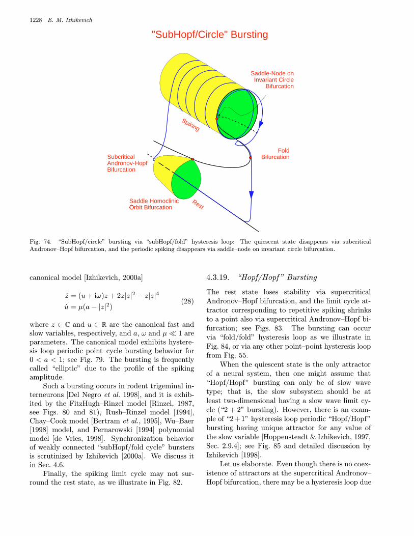
1228 E. M. Izhikevich
Saddle-Node onInvariant Circle
Bifurcation
FoldBifurcation
Spiking
"SubHopf/Circle" Bursting
Rest
SubcriticalAndronov-HopfBifurcation
Saddle HomoclinicOrbit Bifurcation
Fig. 74. “SubHopf/circle” bursting via “subHopf/fold” hysteresis loop: The quiescent state disappears via subcriticalAndronov–Hopf bifurcation, and the periodic spiking disappears via saddle–node on invariant circle bifurcation.
canonical model [Izhikevich, 2000a]
z = (u+ iω)z + 2z|z|2 − z|z|4
u = µ(a− |z|2)(28)
where z ∈ C and u ∈ R are the canonical fast andslow variables, respectively, and a, ω and µ 1 areparameters. The canonical model exhibits hystere-sis loop periodic point–cycle bursting behavior for0 < a < 1; see Fig. 79. The bursting is frequentlycalled “elliptic” due to the profile of the spikingamplitude.
Such a bursting occurs in rodent trigeminal in-terneurons [Del Negro et al. 1998], and it is exhib-ited by the FitzHugh–Rinzel model [Rinzel, 1987,see Figs. 80 and 81), Rush–Rinzel model [1994],Chay–Cook model [Bertram et al., 1995], Wu–Baer[1998] model, and Pernarowski [1994] polynomialmodel [de Vries, 1998]. Synchronization behaviorof weakly connected “subHopf/fold cycle” burstersis scrutinized by Izhikevich [2000a]. We discuss itin Sec. 4.6.
Finally, the spiking limit cycle may not sur-round the rest state, as we illustrate in Fig. 82.
4.3.19. “Hopf/Hopf” Bursting
The rest state loses stability via supercriticalAndronov–Hopf bifurcation, and the limit cycle at-tractor corresponding to repetitive spiking shrinksto a point also via supercritical Andronov–Hopf bi-furcation; see Figs. 83. The bursting can occurvia “fold/fold” hysteresis loop as we illustrate inFig. 84, or via any other point–point hysteresis loopfrom Fig. 55.
When the quiescent state is the only attractorof a neural system, then one might assume that“Hopf/Hopf” bursting can only be of slow wavetype; that is, the slow subsystem should be atleast two-dimensional having a slow wave limit cy-cle (“2 + 2” bursting). However, there is an exam-ple of “2+ 1” hysteresis loop periodic “Hopf/Hopf”bursting having unique attractor for any value ofthe slow variable [Hoppensteadt & Izhikevich, 1997,Sec. 2.9.4]; see Fig. 85 and detailed discussion byIzhikevich [1998].
Let us elaborate. Even though there is no coex-istence of attractors at the supercritical Andronov–Hopf bifurcation, there may be a hysteresis loop due

Neural Excitability, Spiking and Bursting 1229
x
u
FoldBifurcation
Rest
Spiking
Fold LimitCycle
Bifurcation
Fold LimitCycle
Fold
SaddleHomoclinic
Orbit
"Hopf/Fold Cycle" Bursting
0 100 200 300 400 500 600 700 800 900 10000
0.1
0.2
0.3
0.4
0.5
0.6
0.7
0.8
0.9
1
x(t)
SupercriticalAndronov-Hopf
SaddleHomoclinicOrbitBifurcation
SupercriticalAndronov-HopfBifurcation
Fig. 75. “Hopf/fold cycle” bursting via “fold/fold cycle” hysteresis loop: The quiescent state disappears via supercriticalAndronov–Hopf bifurcation, and the periodic spiking disappears via fold limit cycle bifurcation. Simulations of the Wilson–Cowan [1972] model with parameters as in Fig. 68 except ry = −9.7, µ = 0.5, and u = µ(0.745 − x)
√x(u+ 0.05).

1230 E. M. Izhikevich
x
u
FoldBifurcation
FoldBifurcation
Rest
Spiking
SupercriticalAndronov-Hopf
Bifurcation
SubcriticalAndronov-HopfBifurcation
"SubHopf/Hopf" Bursting
Fold LimitCycleBifurcation
0 500 1000 1500 2000 2500 3000
-0.5
-0.4
-0.3
-0.2
-0.1
0
0.1
V(t)
Fold
Fold
Supercritical
Andronov-Hopf
SubcriticalAndronov-Hopf
FoldLimitCycle
Fig. 76. “SubHopf/Hopf” bursting via “fold/fold” hysteresis loop: The quiescent state loses stability via subcritical Andronov–Hopf bifurcation, and the periodic spiking disappears via supercritical Andronov–Hopf bifurcation.
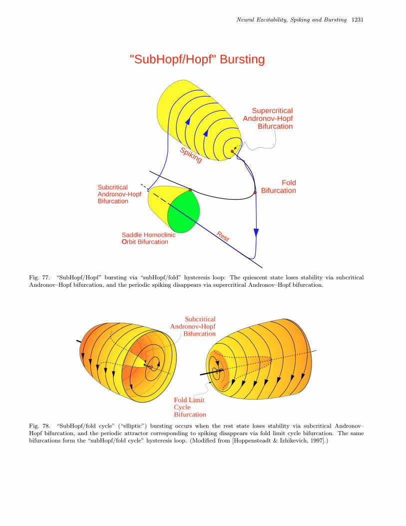
Neural Excitability, Spiking and Bursting 1231
Spiking
"SubHopf/Hopf" Bursting
FoldBifurcation
SupercriticalAndronov-Hopf
Bifurcation
Rest
SubcriticalAndronov-HopfBifurcation
Saddle HomoclinicOrbit Bifurcation
Fig. 77. “SubHopf/Hopf” bursting via “subHopf/fold” hysteresis loop: The quiescent state loses stability via subcriticalAndronov–Hopf bifurcation, and the periodic spiking disappears via supercritical Andronov–Hopf bifurcation.
Fold LimitCycleBifurcation
SubcriticalAndronov-Hopf
Bifurcation
Fig. 78. “SubHopf/fold cycle” (“elliptic”) bursting occurs when the rest state loses stability via subcritical Andronov–Hopf bifurcation, and the periodic attractor corresponding to spiking disappears via fold limit cycle bifurcation. The samebifurcations form the “subHopf/fold cycle” hysteresis loop. (Modified from [Hoppensteadt & Izhikevich, 1997].)

1232 E. M. Izhikevich
0 u
1
-1
r
Re z(t)
r(t)
0 u
1
-1
r
Re z(t)
r(t)
Slow PassageEffect
Fig. 79. Phase portrait and solution of the canonical model (28) for µ = 0.1, ω = 3, and a = 0.25 (top) and a = 0.8 (bottom).Modified from [Izhikevich, 2000a].
0
2
-2
0
1
0.01
0.02y
v
w
250Time
v(t)
Fig. 80. FitzHugh–Rinzel model of “subHopf/fold cycle” bursting (from [Izhikevich, 2000a]).
Premature ReentrySlow Passage Effect
Fig. 81. Slow passage effect and premature reentry in the FitzHugh–Rinzel model of “subHopf/fold cycle” bursting. Thelatter likely contributes to the apparent irregularity of bursting (from [Izhikevich, 2000a]).
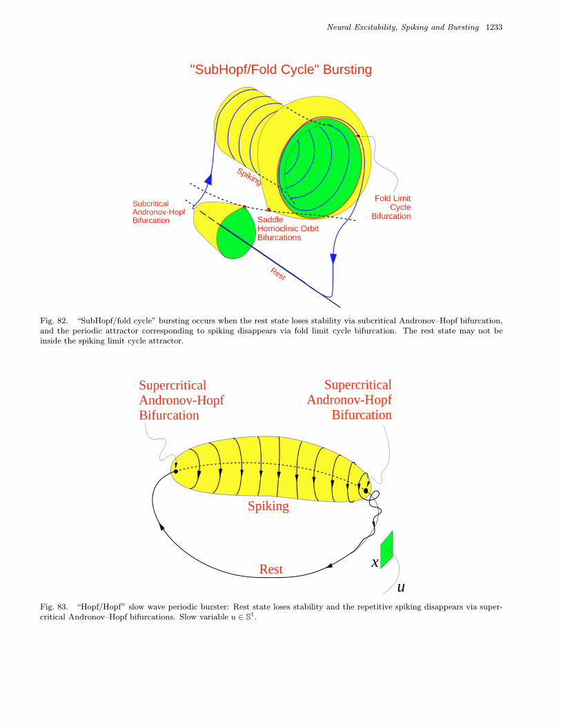
Neural Excitability, Spiking and Bursting 1233
Rest
SubcriticalAndronov-HopfBifurcation
Spiking
Fold LimitCycle
Bifurcation
"SubHopf/Fold Cycle" Bursting
SaddleHomoclinic OrbitBifurcations
Fig. 82. “SubHopf/fold cycle” bursting occurs when the rest state loses stability via subcritical Andronov–Hopf bifurcation,and the periodic attractor corresponding to spiking disappears via fold limit cycle bifurcation. The rest state may not beinside the spiking limit cycle attractor.
Rest
Spiking
u
x
SupercriticalAndronov-HopfBifurcation
SupercriticalAndronov-Hopf
Bifurcation
Fig. 83. “Hopf/Hopf” slow wave periodic burster: Rest state loses stability and the repetitive spiking disappears via super-critical Andronov–Hopf bifurcations. Slow variable u ∈ S1.

1234 E. M. Izhikevich
u
SupercriticalAndronov-Hopf
Bifurcation
x
Spiking
Rest
Fold
Fold
SupercriticalAndronov-Hopf
0 200 400 600 800 1000 1200 1400 1600 1800 2000-0.7
-0.6
-0.5
-0.4
-0.3
-0.2
-0.1
0
0.1
V(t)
SupercriticalAndronov-Hopf
"Hopf/Hopf" Bursting
Fig. 84. “Hopf/Hopf” bursting via “fold/fold” hysteresis loop. Transitions between periodic spiking and quiescence occurvia supercritical Andronov–Hopf bifurcations.

Neural Excitability, Spiking and Bursting 1235
t
0.5
u
x
x
1
2
x1Supercritical Andronov-Hopf Bifurcation
u
|x|
S
0.5
u
Slow PassageEffect
Fig. 85. “Hopf/Hopf” hysteresis loop periodic bursting in x = (u + i)x − x|x|2, u = µ(2λS(u/λ − λ) − |x|), where x =x1 + ix2 ∈ C, u ∈ R, µ = 0.05, λ =
√µ/20 and S(ρ) = 1/(1 + e−ρ). The hysteresis loop is due to the slow passage effect, not
due to the coexistence of attractors (from [Hoppensteadt & Izhikevich, 1997]). This burster is “2 + 1”.
to the phenomenon knows as ramp effect, memoryeffect, or effect of slow passage through the bifur-cation [Nejshtadt, 1985; Baer et al., 1989; Holden& Erneux, 1993a, 1993b; Arnold et al., 1994]. Themechanism of supercritical elliptic bursting havingone-dimensional slow subsystem can be explained asfollows: When x is close to a rest state, the variableu increases and passes slowly through the bifurca-tion value. Due to the slow passage, the fast vari-able x remains to be close to the rest equilibriumeven after u passed the bifurcation value. After awhile x diverges from the rest potential and startsto oscillate, in which case u decreases (relativelyquickly) and passes through the bifurcation in theopposite direction thereby completing the hysteresisloop, as in the upper-left corner of Fig. 85.
One should be warned though that the slowpassage effect is very sensitive to nonsmoothness ofthe system and to noise. Thus, however ubiquitousthis type of bursting can be in computer simula-tions, it may never be encountered experimentally.
The example of hysteresis loop “Hopf/Hopf”bursting depicted in Fig. 85 shows how cautiousone should be when averaging bursting systems.
Indeed, if the fast subsystem has a unique attractor,and the slow subsystem is one-dimensional, then theaveraged system (22) is one-dimensional, and hencecannot oscillate. Therefore hysteresis loop periodicbursting in (21) is impossible. This argument failsbecause (22) describes accurately (21) on the timescale of order 1/µ or less, unless other restrictionsare imposed. But the time required for convergenceof x(t) to the unique attractor might be larger than1/µ due to the slow passage effect. Moreover, theaveraged system (22) is not Lipchitz since x(t, u)behaves like
√u near the Andronov–Hopf bifurca-
tion point u = 0. Thus, not only (22) is a badapproximation to (21), but also it has nonunique so-lutions. Therefore, averaging fails to provide goodintuition for such bursting.
4.3.20. Subtypes
Let us use the “fold/homoclinic” bursting to illus-trate the issue raised by Bertram et al. [1995]: Thelarge amplitude limit cycle attractor correspond-ing to periodic spiking may encompass the qui-escent state, which happens, e.g. during the big

1236 E. M. Izhikevich
0 500 1000 15002
1.5
1
0.5
0
0.5
1
1.5
2
FoldBifurcation
Spiking
V(t)
Fold Big SaddleHomoclinic Orbit
"Fold/BIG Homoclinic" Bursting
Big SaddleHomoclinic OrbitBifurcations
Rest
Fig. 86. “Fold/big homoclinic” (“square-wave”) bursting: The rest state disappears via fold bifurcation and the limit cycledisappears via big saddle homoclinic orbit bifurcation. Simulations of (15) with a(u) = −u, b = 1.75, c = −0.5, d = 0.1,ε = 0.15, and the slow subsystem u = µ(0.5 + v) with µ = 0.0005.

Neural Excitability, Spiking and Bursting 1237
Saddle-Node onInvariant Circle
Bifurcation
FoldBifurcation
Rest
Spiking
"SubHopf/Circle" Bursting
SubcriticalAndronov-HopfBifurcation
Saddle HomoclinicOrbit Bifurcation
Rest
Spiking
Saddle-Node on InvariantCircle Bifurcations
FoldBifurcation
FoldBifurcation
"Circle/Circle" Bursting
"Circle/BIG Homoclinic" Bursting
Big SaddleHomoclinic OrbitBifurcation
Rest
FoldBifurcation
Saddle-Node on InvariantCircle Bifurcation
Saddle-Node onInvariant Circle
Bifurcation
FoldBifurcation
FoldBifurcation
Rest
Spiking
"Fold/Circle" Bursting
FoldBifurcation
Spiking
Fold LimitCycle
Bifurcation
"Fold/Fold Cycle" Bursting
Rest
Big SaddleHomoclinic OrbitBifurcation
"SubHopf/BIG Homoclinic" Bursting
Big SaddleHomoclinic OrbitBifurcation
Rest
SaddleHomoclinic OrbitBifurcation
SubcriticalAndronov-HopfBifurcation
Spiking
Spiking
Fig. 87. The large amplitude limit cycle attractor corresponding to repetitive spiking can surround the rest state.

1238 E. M. Izhikevich
SaddleHomoclinic Orbit
SaddleHomoclinic Orbit
"Homoclinic/BIG Homoclinic" Bursting
0 50 100 150 200 250 300 350 400 4502
1.5
1
0.5
0
0.5
1
1.5
v(t)
SaddleHomoclinic OrbitBifurcations
Fig. 88. “Homoclinic/homoclinic” cycle–cycle bursting: The transitions between quiescent and spiking limit cycles occur viasaddle homoclinic orbit bifurcations. The same bifurcations form the hysteresis loop. Simulations of (15) with a(u) = −u,b = 1.3, c = −0.32, d = 0.05, ε = 1, slow subsystem u = µ(0.4 + v) and µ = 0.01.

Neural Excitability, Spiking and Bursting 1239
Spiking
SaddleHomoclinic
OrbitBifurcation
"Homoclinic/Homoclinic" Bursting
x
u
SaddleHomoclinic OrbitBifurcation
Rest
Fig. 89. “Homoclinic/homoclinic” cycle–cycle bursting: The transitions between quiescent and spiking limit cycles occur viasaddle homoclinic orbit bifurcations, which form a hysteresis loop.
saddle homoclinic orbit bifurcation; see Figs. 32 and86. Bertram et al. [1995] suggested to refer to such“fold/homoclinic” bursting as being Type Ib, as op-posed to “regular” Type Ia. The “fold/big homo-clinic” bursting is not an exception: Other burstersmay have the same property, as we illustrate inFig. 87. Even though the new types are equiva-lent to the old ones from the purely mathematicalpoint of view, it may still be useful to distinguish be-tween them, since they might have different neuro-computational properties.
Finally, the distinction may have limited valuewhen the fast subsystem has dimension 3 and up,since the notions surround or in between may notbe well defined there.
4.4. Planar Cycle cycle bursting
Next, we give examples of some cycle–cycle planarbursters.
4.4.1. “Homoclinic/homoclinic” bursting
The transitions from quiescent to spiking limitcycles and back occur via saddle homoclinic orbitbifurcations; see Figs. 88 and 89.
4.4.2. “Homoclinic/Hopf” bursting
The quiescent limit cycle disappears via saddle ho-moclinic orbit bifurcation and the spiking limit cy-cle shrinks to a point via supercritical Andronov–Hopf bifurcation; see Fig. 90.
4.4.3. “Homoclinic/fold cycle” bursting
The quiescent limit cycle disappears via saddle ho-moclinic orbit bifurcation and the spiking limit cy-cle disappears via fold limit cycle bifurcation; seeFig. 91.
4.4.4. “Homoclinic/circle” bursting
The quiescent limit cycle disappears via saddle ho-moclinic orbit bifurcation and the spiking limit cy-cle disappears via saddle–node on invariant circlebifurcation; see Fig. 92.
4.4.5. “Fold cycle/fold cycle” bursting
The transitions between quiescent and spiking limitcycle attractors occur via fold limit cycle bifurca-tions; see Figs. 93 and 94. This is the only type of

1240 E. M. Izhikevich
0 50 100 150 200 250 300 350 400 450 500 5502
1.5
1
0.5
0
0.5
1
1.5
SaddleHomoclinic Orbit Fold
"Homoclinic/Hopf" Bursting
v(t)
Supercritical
Andronov-Hopf
x
u
FoldBifurcation
SaddleHomoclinic OrbitBifurcation
Rest
Spiking
SupercriticalAndronov-Hopf
Bifurcation
Fig. 90. “Homoclinic/Hopf” cycle–cycle bursting via “homoclinic/fold” hysteresis loop: The quiescent oscillation disappearsvia saddle homoclinic orbit bifurcation and the periodic spiking disappears via supercritical Andronov–Hopf bifurcation.Simulations of (15) with a(u) = −0.77 − 0.33u/(u + 0.15), b(u) = 1.65 + u, c = −0.15 + u, d = 0.1, ε = 1, slow subsystemu = µv and µ = 0.01.

Neural Excitability, Spiking and Bursting 1241
Spiking
Fold Limit CycleBifurcation
"Homoclinic/Fold Cycle" Bursting
x
u
SaddleHomoclinic OrbitBifurcation
Rest
Fig. 91. “Homoclinic/fold cycle” bursting: The quiescent oscillation disappears via saddle homoclinic orbit bifurcation andthe periodic spiking disappears via fold limit cycle bifurcation. The same bifurcations form the hysteresis loop.
"Homoclinic/Circle" Bursting
x
u
SaddleHomoclinic OrbitBifurcation
Rest
Saddle-Node onInvariant Circle
Bifurcation
FoldBifurcation
Spiking
Fig. 92. “Homoclinic/circle” cycle–cycle bursting via “homoclinic/fold” hysteresis loop: The quiescent oscillation disappearsvia saddle homoclinic orbit bifurcation and the periodic spiking disappears via saddle–node on invariant circle bifurcation.

1242 E. M. Izhikevich
Spiking
Fold Limit CycleBifurcation
"Fold Cycle/Fold Cycle" Bursting
x
u
Rest
Fold LimitCycleBifurcation
Saddle HomoclinicOrbit Bifurcations
Fig. 93. “Fold cycle/fold cycle” bursting: The transitionsbetween quiescent and spiking oscillations occur via fold limitcycle bifurcations, which form a hysteresis loop.
Fold LimitC
ycle
Bifurcations
"Fold Cycle/Fold Cycle" Bursting
Fig. 94. “Fold cycle/fold cycle” bursting: The transitionsbetween quiescent and spiking oscillations occur via fold limitcycle bifurcations, which form a hysteresis loop.
f(r,u)=0
g(r,u)=0
r
u
0
Fig. 95. Typical intersections of nullclines in “fold cycle/foldcycle” hysteresis loop bursting: r > 0 is the amplitude of fastoscillation, u is the slow variable.
cycle–cycle bursting for which rigorous asymptotictheory exists [Mishchenko et al., 1994]. “Foldcycle/fold cycle” bursting can be seen in theHodgkin–Huxley-like models by Shorten and Wall[2000] and Wang [1993]. The latter also exhibits“fold cycle/flip” bursting.
An easy way to make a simple example of “foldcycle/fold cycle” burster is to take any standardrelaxation system
r = f(r, u)
u = µg(r, u)
having N -shaped fast nullcline that intersects theslow nullcline at one point (see Fig. 95) and assumethat r is the amplitude of fast oscillation. The vari-
able z(t) = r(t)eiωt would exhibit “fold cycle/foldcycle” hysteresis loop bursting. Thus, most of theresults devoted to studying synchronization prop-erties of relaxation oscillators (see e.g. [Belair &Holmes, 1984; Storti & Rand, 1986; Grasman, 1987;Somers & Kopell, 1993, 1995; Kopell & Somers,1995; Terman & Wang, 1995; Terman & Lee, 1997;Izhikevich, 2000b]) can immediately be generalizedto that of “fold cycle/fold cycle” bursters.
There is a relationship between the “foldcycle/fold cycle” and “subHopf/fold cycle”(“elliptic”) bursting: When the latter has a fastsubsystem near Bautin bifurcation and it receivesweak time-dependent input, it is described by thecanonical model [Izhikevich, 1999]
r = b+ r + 2r3 + r5
ϕ = ω
u = µ(a− r2)
(29)
where z = reiϕ ∈ C, which coincides with (28) whenb = 0. Its typical “fold cycle/fold cycle” burstingsolution is depicted in Fig. 96.

Neural Excitability, Spiking and Bursting 1243
0 10 20 30 40 50 60 70 80 90 1001.5
1
0.5
0
0.5
1
1.5
Re z(t)
Fig. 96. A typical “fold cycle/fold cycle” bursting solution of (29). Parameters: a = 0.5, b = 0.1, ω = 3, µ = 0.1.
x
u
Rest
Spiking
SaddleHomoclinic Orbit
Bifurcation
"Fold Cycle/Homoclinic" Bursting
Fold LimitCycleBifurcation
Fig. 97. “Fold cycle/homoclinic” cycle–cycle bursting: Thequiescent state disappears via fold limit cycle bifurcation andthe spiking state disappears via saddle homoclinic orbit bi-furcation. The same bifurcations form the hysteresis loop.
4.4.6. “Fold cycle/homoclinic” bursting
The quiescent oscillation disappears via fold limitcycle bifurcation and the spiking oscillation disap-pears via saddle homoclinic orbit bifurcation; seeFig. 97.
4.4.7. “Fold cycle/circle” bursting
The quiescent oscillation disappears via fold limitcycle bifurcation and the spiking oscillation disap-pears via saddle–node on invariant circle bifurca-tion; see Fig. 98.
4.4.8. “Fold cycle/Hopf” bursting
The quiescent oscillation disappears via fold limitcycle bifurcation and the spiking oscillation shrinks
x
u
Rest
Fold LimitCycleBifurcation
Saddle-Node onInvariant Circle
Bifurcation
FoldBifurcation
Spiking
"Fold Cycle/Circle" Bursting
Fig. 98. “Fold cycle/circle” bursting via “fold cycle/fold”hysteresis loop: The quiescent state disappears via fold limitcycle bifurcation and the spiking state disappears via saddle–node on invariant circle bifurcation.
to a point via supercritical Andronov–Hopf bifurca-tion; see Fig. 99.
4.5. Intermediate µ
The basic idea behind the dissection of the fast–slow bursting is that the relaxation parameter µ in(21) is as small as we wish so that the slow vari-able u may be assumed to be static on the fast timescale. In practice, µ may not be infinitesimal, butmay assume intermediate values; e.g. µ = 0.1 in
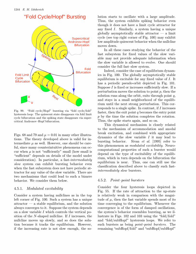
1244 E. M. Izhikevich
x
u
Rest
Fold LimitCycleBifurcation
Spiking
"Fold Cycle/Hopf" Bursting
FoldBifurcation
SupercriticalAndronov-Hopf
Bifurcation
Fig. 99. “Fold cycle/Hopf” bursting via “fold cycle/fold”hysteresis loop: The quiescent state disappears via fold limitcycle bifurcation and the spiking state disappears via super-critical Andronov–Hopf bifurcation.
Figs. 68 and 79 and µ = 0.01 in many other illustra-tions. The theory developed above is valid for in-termediate µ as well. However, one should be care-ful, since many counterintuitive phenomena can oc-cur when µ is not “sufficiently” small (how small is“sufficient” depends on details of the model underconsideration). In particular, a fast-intermediatelyslow system can exhibit bursting behavior evenwhen the fast subsystem does not have periodic at-tractor for any value of the slow variable. There aretwo mechanisms that could lead to such a bizarrebehavior. We consider them below.
4.5.1. Modulated excitability
Consider a system having nullclines as in the topleft corner of Fig. 100. Such a system has a uniqueattractor — a stable equilibrium, and the solutionalways converges to it. Suppose the system dependson a slow variable I which controls the vertical po-sition of the N -shaped nullcline. If I increases, thenullcline moves up slowly, and so does the solu-tion because it tracks the equilibrium. However,if the increasing rate is not slow enough, the so-
lution starts to oscillate with a large amplitude.Thus, the system exhibits spiking behavior eventhough it does not have a limit cycle attractor forany fixed I. Similarly, a system having a uniqueglobally asymptotically stable attractor — a limitcycle (see top right corner of Fig. 100) may exhibitlow amplitude quiescent behavior when the nullclinemoves down.
In all these cases studying the behavior of thefast subsystem for fixed values of the slow vari-able may not provide adequate information whenthe slow variable is allowed to evolve. One shouldconsider the full fast–slow system.
Indeed, consider the case of equilibrium dynam-ics in Fig. 100. The globally asymptotically stableequilibrium is excitable for any fixed value of I. Ithas a periodic pseudo-orbit depicted in Fig. 101.Suppose I is fixed or increases sufficiently slow. If aperturbation moves the solution to point p, then thesolution runs along the orbit, exits through point q,and stays in a small neighborhood of the equilib-rium until the next strong perturbation. This cor-responds to a single spike. In contrast, if I increasesfaster, then the exit point q becomes the entry pointp by the time the solution completes the rotation.Thus, the spike starts again, and so on.
This dynamical mechanism is closely relatedto the mechanism of accommodation and anodalbreak excitation, and combined with appropriatedynamics of the slow variable I it may lead tobursting behavior. Sivan et al. [1995] refer tothis phenomenon as modulated excitability. Neuro-computational properties of such a burster woulddepend on the type of excitability of the equilib-rium, which in turn depends on the bifurcation theequilibrium is near. Thus, one can still use theclassification described above to classify such fast-intermediately slow bursters.
4.5.2. Point–point bursters
Consider the four hysteresis loops depicted inFig. 55. If the rate of attraction to the up-stateis relatively weak in comparison with the magni-tude of µ, then the fast variable spends most of itstime converging to the equilibrium. Whenever theconvergence is of the form of damped oscillations,the system’s behavior resembles bursting, as we il-lustrate in Figs. 102 and 103 using the “fold/fold”and “fold/subHopf” hysteresis loops. We refer tosuch bursters as being point–point bursters. Theremaining “subHopf/fold” and “subHopf/subHopf”

Neural Excitability, Spiking and Bursting 1245
2.5 2 1.5 1 0.5 0 0.5 1 1.5 2 2.52.5
2
1.5
1
0.5
0
0.5
1
1.5
2.5 2 1.5 1 0.5 0 0.5 1 1.5 2 2.52.5
2
1.5
1
0.5
0
0.5
1
1.5
2.5 2 1.5 1 0.5 0 0.5 1 1.5 2 2.52.5
2
1.5
1
0.5
0
0.5
1
1.5
2.5 2 1.5 1 0.5 0 0.5 1 1.5 2 2.51
0.5
0
0.5
1
1.5
2
2.5
2.5 2 1.5 1 0.5 0 0.5 1 1.5 2 2.51
0.5
0
0.5
1
1.5
2
2.5
2.5 2 1.5 1 0.5 0 0.5 1 1.5 2 2.51
0.5
0
0.5
1
1.5
2
2.5
Equilibrium Dynamics Periodic Dynamics
µ=0
µ=0.01µ=0.01
µ=0.005
µ=0
µ=0.005
Rest
SpikingRest
Spiking
Fig. 100. Left: The system has a unique attractor — equilibrium, yet it can exhibit repetitive spiking activity when the N-shaped nullcline is moved up. Right: The system has a unique attractor — limit cycle, yet it can exhibit low amplitude quiescentactivity when the N-shaped nullcline is moved down. Simulations of the Bonhoeffer–Van Der Pol oscillator x = I+x−x3/3−y,y = ε(x+ a) for ε = 0.1, a = 1.05 (left) or a = 0.9 (right), and I = µ.
point–point bursters are illustrated elsewhere. Itis remarkable that periodic bursting may occur de-spite the fact that the fast subsystem does not havea limit cycle attractor for any value of the slowvariable.
It is believed that the “fold/subHopf” hystere-sis loop point–point bursting is exhibited by thepituitary somatotroph cells, which secrete growthhormone [A. Sherman & A. LeBeau, personalcommunication].
4.6. Synchronization of bursters
In this section we consider a weakly connected sys-tem of the form
xi = fi(xi, ui) + εpi(x, u, ε) (30)
ui = µ[gi(xi, ui) + εqi(x, u, ε)] (31)
where x = (x1, . . . , xn) ∈ Rmn and u =(u1, . . . , un) ∈ Rkn are vectors of the fast and slow

1246 E. M. Izhikevich
2.5 2 1.5 1 0.5
0
0.5
1 1.5 2 2.51
0.5
0
0.5
1
1.5
p
qPseudo-Orbit
StableEquilibrium
Fig. 101. A periodic pseudo-orbit in Bonhoeffer–Van DerPol oscillator from Fig. 100 having (excitable) asymptoti-cally stable equilibrium; i.e. a piece of solution starting froma point p and exiting at a nearby point q.
variables, respectively, and ε 1 is the strength ofconnections. We assume that each subsystem
xi = fi(xi, ui)
ui = µgi(xi, ui)
exhibits periodic hysteresis loop bursting behav-ior. We also assume that the coupling is relativelystrong in comparison with the magnitude of µ; thatis,
µ = O(ε) ,
which also includes the case µ ε. The case ofextremely weak coupling (µ ε) is not interestingfor our discussion here.
There are two rhythmic processes associatedwith each burster: repetitive spiking and repeti-tive bursting. Therefore, there could be at leasttwo different regimes of synchronization, which aredepicted in Fig. 104:
• Synchronization of individual spikes.• Synchronization of bursts.
One of them does not imply the other. Of course,there is an additional regime when both types ofsynchronization occur simultaneously.
4.6.1. Spike synchronization
A naive approach to study spike synchronizationis to consider the fast subsystem (30), which is
a weakly connected network of limit cycle oscil-lators. In Sec. 3.5 we show that the oscillatorscannot lock unless they have nearly equal or low-order resonant frequencies. Thus, synchronizationof individual spikes within a single burst dependscrucially on the interspike frequencies. The fre-quencies, however, may vary substantially duringthe burst, because they depend on the values ofthe slow variables u1, . . . , un. A rigorous averag-ing theory for such systems is quite complicated[Arnold, 1982].
Spike synchronization may occur during the en-tire duration of a burst, or during the initial or thefinal stage of the burst. We present a nonrigorousdiscussion of these cases below.
4.6.1.1. Initial stage
Spike synchronization during the initial stage ofthe burst usually does not occur between “circle/*”bursters (where “*” means a wildcard) becauseof the following two reasons: (i) The interspikefrequency changes substantially during the initialstage. Hence, small deviations in the values of theslow variables may lead to drastic variances in thefrequencies. (ii) The canonical model for Class 1systems (11) does not exhibit stable locking. Sim-ilar arguments can be applied to the “blue-sky/*”and “torus/*” bursters.
The other types of bursters tend to have reg-ular spiking during the initial stage of a burst.Therefore, they could exhibit spike synchronization.However, the convergence to the synchronized statetakes as many as O(1/ε) spikes, and can be longerthan the entire initial stage.
4.6.1.2. Final stage
Using nonrigorous arguments similar to those pre-sented above, one can conclude that “*/circle”,“*/blue-sky”, and “*/torus” bursters do not usu-ally exhibit spike synchronization during the finalstage of the burst.
The case of “*/* homoclinic” bursting is sub-tler. The interspike frequency decreases as the func-tion 1/| ln λ| (see Table 2), which does not seem tovanish unless the distance to the bifurcation, λ, isvery small. Hence, the sudden drop in the inter-spike frequency occurs during the last few spikes,which may lead to their desynchronization, as onecan see in Fig. 106.

Neural Excitability, Spiking and Bursting 1247
0 100 200 300 400 500 600-2
-1.5
-1
-0.5
0
0.5
1
1.5
2
x
u
FoldBifurcation
Up-State(Rest)
Down-State(Rest)
FoldBifurcation
"Fold/Fold" Bursting
v(t)
Fold
Fold
Fig. 102. “Fold/fold” hysteresis loop bursting of point–point type. Notice that the fast subsystem does not have a limit cycleattractor for any value of the slow variable. Bursting occurs because the rate of convergence to the up-state is relatively weak.Shown are simulations of the model (15) with parameters of the slow subsystem c = µv. Parameters: (a, b, d, ε, µ) = (−1.3,2.3, 0.1, 0.5, 0.01).

1248 E. M. Izhikevich
0
20 40 60 80 100
120-0.6
-0.5
-0.4
-0.3
-0.2
-0.1
0
0.1
0.2
0.3
0.4
v(t)
FoldBifurcation Saddle Homoclinic
Orbit Bifurcation
SubcriticalAndronov-Hopf
Bifurcation
"Fold/SubHopf" Bursting
x
u
Up-State(Rest)
Down-State(Rest)
Fold Saddle HomoclinicOrbit Bifurcation
SubcriticalAndronov-Hopf
Bifurcation
Fig. 103. “Fold/subHopf” hysteresis loop bursting of point–point type. The fast subsystem does not have a limit cycleattractor for any value of the slow variable. Bursting occurs because the rate of convergence to the up-state is relativelyweak. Shown are simulations of the Morris–Lecar model (25) with I(u) = −u and the slow subsystem u = µV . Parameters:V3 = 0.107, V4 = 0.07, gCa = 1.33, µ = 1/8, the rest as in Fig. 59.

Neural Excitability, Spiking and Bursting 1249
Spike Synchronization
Burst Synchronization
Fig. 104. Various regimes of synchronization of bursters(modified from [Izhikevich, 2000a]).
4.6.2. Burst synchronization
Dynamics of burst synchronization of weakly cou-pled bursters is similar in some aspects to that ofstrongly coupled relaxation oscillators.
To understand the mechanism of stable burstsynchronization we consider two planar point–cyclebursters: One in the active (spiking) state, andthe other still in the quiescent down-state. If theactive burster makes the quiescent burster jumpfrom the down-state prematurely, then they mayexhibit stable burst synchronization. If it prolongsthe quiescent down-state, then the in-phase burstsynchronization cannot be stable, but some otherregime, such as anti-phase burst synchronization,may occur.
We distinguish two mechanisms that lead tostable burst synchronization depending on whetherthe quiescent burster is an integrator or a resonator.
4.6.2.1. Integrators
If point–cycle bursting occurs via “fold/*” hys-teresis loop, then the burster acts as an integra-tor. While the slow variable is near the bifurcationvalue, the fast variable is ready to jump up in re-sponse to incoming pulses from the active burster.This jump may lead to repetitive spiking when the
Rest
Spiking
Excitatory Stimulation
Inhibitory Stimulation
Fig. 105. Excitatory (inhibitory) pulses shorten (lengthen)the quiescent state in “fold/*” hysteresis loop bursters. Thismay lead to burst synchronization (desynchronization).
bursting is of “fold/*” type, or to the up-state whenthe bursting is of “circle/*” or “Hopf/*” type. Inany case the jump shortens the quiescent phase.
If the synaptic connections are excitable, thequiescent burster does jump prematurely. Thehigher the frequency of the incoming pulses,the sooner it jumps. In contrast, if the connec-tions are inhibitory, the quiescent down-state is pro-longed; see Fig. 105.
Shortening the quiescent state is necessary butnot sufficient condition for stable synchronization.The latter has yet to be found; It will depend onthe bifurcation of the spiking state, and probably besimilar to the compression hypothesis in the FastThreshold Modulation (FTM) theory of synchro-nization of strongly connected relaxation oscillators[Somers & Kopell, 1993, 1995]: The rate of changeof slow variable before the jump is less than thatafter the jump. In this case the bursters may be-have according to a simple rule excitation meanssynchronization, inhibition means desynchroniza-tion, as we illustrate in Fig. 106.

1250 E. M. Izhikevich
Uncoupled
Excitatory Coupling
Inhibitory Coupling
SpikeSynchronization
SpikeDe-Synch-ronization
Fig. 106. Burst synchronization and desynchronization in“fold/homoclinic” (“square-wave”) bursters. Shown are sim-ulations of coupled Morris–Lecar systems with additionalslow variables.
4.6.2.2. Resonators
If point–cycle bursting occurs via “subHopf/*” hys-teresis loop, then the burster acts as a resonator inthe quiescent down-state. Such a burster exhibitsdamped subthreshold oscillations of the membranepotential, see Sec. 2.2. If the frequency of the in-coming pulses is resonant with the frequency of thesubthreshold oscillation, then the quiescent bursterjumps up prematurely, which may result in stablein-phase burst synchronization. The lower the orderof resonance is, the sooner it jumps, as we illustratein Fig. 107. If the input pulse train is not resonant,the quiescent down-state is not affected.
A seemingly counterintuitive observation isthat the sign of synapse does not affect burst syn-chronization, but may only affect spike synchroniza-tion, as we illustrate in Fig. 108. This observationagrees with the fact that a resonator can fire in re-sponse to excitatory as well as inhibitory pulse, aswe discuss in Sec. 2.2. Therefore, in contrast to
1:2 Resonance
3:8 Resonance
No Resonance
1:4 Resonance
Fig. 107. The response of the “SubHopf/fold cycle”(“elliptic”) burster (black) depends on the frequency of theincoming pulses (red). Lower-order resonances produce ear-lier responses. Shown are simulations of excitatory coupledFitzHugh–Rinzel bursters [Izhikevich, 2000a].
the previously discussed case, both excitation andinhibition can lead to burst synchronization.
4.6.3. Delayed onset of bursting
There is an interesting phenomenon that is ubiqui-tous in computer simulations of bursters but maynever be encountered in experiments: The onset ofbursting can be delayed significantly when the vari-able u passes slowly a bifurcation value. That is,the fast variable remains quiescent despite the factthat the slow variable has already crossed the bi-furcation value and the quiescent state has alreadybecome unstable or disappeared. Because such aquiescence is highly unstable, small perturbationsfrom the other bursters can cause an immediatetransition to the active state, which may result ininstantaneous synchronization.
There are two different but related mechanismsfor such a delay.
4.6.3.1. Slow passage effect
First, consider the case when the quiescent stateloses stability, e.g. via an Andronov–Hopf bifurca-

Neural Excitability, Spiking and Bursting 1251
Uncoupled
EcxitatoryConnection
InhibitoryConnection
Fig. 108. The type of synaptic connection does not af-fect burst synchronization in coupled “SubHopf/fold cycle”(“elliptic”) bursters. It affects only the spike synchronization,which is in-phase for excitatory synapses and anti-phase forinhibitory synapses. Shown are simulations FitzHugh–Rinzelbursters [Izhikevich, 2000a].
t
t
t
x
x
Andronov-HopfBifurcation
SlowPassageEffect
u
Fig. 109. Slow passage through Andronov–Hopf bifurcation.(Modified from [Hoppensteadt & Izhikevich, 1997].)
tion. When the rest state becomes unstable, thefast variable still needs some time to diverge fromthe equilibrium, which can be significant, as we il-lustrate in Fig. 109. We encounter this phenomenonwhen we consider “Hopf/Hopf” and “SubHopf/foldcycle” bursting. The slow passage effect can also beobserved near Neimark–Sacker bifurcation.
The slow passage effect is very sensitive towhether or not the system is analytical [Nejshtadt,1985]. Many mathematical models of bursters areanalytical, and hence they exhibit such an effect incomputer simulations. However, the effect can be amathematical artifact, since it has yet to be seen inexperiments.
The slow passage effect can be shortenedsignificantly by noise or weak input from otherbursters. The latter provides a powerful mecha-nism for instantaneous synchronization of bursterseven when they have essentially different interburstfrequencies. For example, a pair of “SubHopf/foldcycle” bursters from Fig. 79 can synchronize in-phase instantaneously (if coupled) because theslower burster spends half of the quiescent time nearthe unstable equilibrium and is ready to fire in re-sponse to the very first pulse coming from the fasterburster.
4.6.3.2. French duck (canard) solutions
When a relaxation system has nullclines intersectedas in Fig. 110, it may have a so-called French duck(canard) periodic solution [Eckhaus, 1983]. Afterthe fast variable reached the left knee point, it doesnot jump to the right branch, but stays near theunstable middle branch for some time. Similar phe-nomenon may occur in “fold/*”, “fold cycle/*”, and“*homoclinic/*” bursters [Booth et al., 1997], as weillustrate in Fig. 111. The fast variable stays nearthe unstable state for some time before jumping tothe limit cycle attractor. A necessary condition forsuch a delayed quiescence is that the slow subsys-tem has an equilibrium near the bifurcation value.That is, the manifold of equilibria of the slow sub-system depicted as a yellow plane in Fig. 111 shouldpass near the left knee point.
The fast variable near the unstable branch ishighly susceptible to small perturbations, e.g. thosecoming from the other bursters. An excitable spikecan make it fire, resulting in instantaneous synchro-nization. In contrast, an inhibitory spike can makeit jump to the lower (stable) branch, thereby delay-ing the onset of bursting even further.

1252 E. M. Izhikevich
Fig. 110. French duck (canard) solutions in relaxationsystems.
x
u
FoldBifurcation
Rest
Spiking
SaddleHomoclinic
OrbitBifurcation
DuckSolution
f(x,u)=0 g(x,u)=0
Fig. 111. The onset of bursting is delayed in the“fold/homoclinic” (“square-wave”) burster due to the Frenchduck (canard) phenomenon.
Since French duck solution exists in a narrowrange of parameters [Arnold et al., 1994], and it issensitive to noise, it is not clear whether the phe-nomenon of delayed onset of bursting can occur inreal cells.
Similarly, we do not discuss here the phe-nomenon of delayed transition to the quiescentstate, which occurs in “*/homoclinic” bursters aswe illustrate in Fig. 112. A tiny transition delay canbe seen in almost all simulations of “*/homoclinic”bursters presented in this paper. A significant de-lay may even affect synchronization properties ofbursters in computer simulations, but it is also un-likely to be encountered in real cells.
"Fold/Homoclinic" Bursting
x
u
FoldBifurcation
Rest
Spiking
SaddleHomoclinic
OrbitBifurcation
DelayedTransition
Fig. 112. Delayed transition to the quiescent state during“fold/homoclinic” bursting.
4.6.4. Rate of locking
The rate of convergence to attractors in weakly con-nected networks is very slow; namely, it is of or-der ε 1, where ε is the strength of connections[Hoppensteadt & Izhikevich, 1997]. For example, aweakly connected oscillatory network (18) needs asmany as O(1/ε) spikes to synchronize2 regardlessof whether each element is a smooth or a relax-ation oscillator. This is the major source of crit-icism of weakly connected models, since the slowrate of convergence contradicts some experimentalobservations. For example, the CPG behavior inthe lamprey is characterized by a strong rate of con-vergence to attractor (see e.g. [Kopell, 1995; Somers& Kopell, 1995; Williams & Sigvardt, 1995]), but itis modeled by a system of phase equations which isa canonical model for weakly connected oscillators.
Our analysis of weakly connected bursters sug-gests that the discrepancy in rates of convergence isnot due to the assumption of weakness of connec-tions, but due to the assumption that each segment
2Under synchronization we mean here convergence to a small but finite neighborhood of an appropriate attractor, which takesO(1/ε) units of time. Complete convergence to the attractor is an asymptotic process that requires infinite amount of time,unless the system is non-Lipchitz or the initial state is on the attractor.

Neural Excitability, Spiking and Bursting 1253
of lamprey spinal cord can be modeled by an oscil-lator. If we model it by a burster, which it is, thenthe rate of convergence to an attractor looks “fast”compared to the interburst period despite the factthat the bursters are weakly connected. Indeed, ittakes O(1/ε) spikes to produce O(1) changes in theactivity of a postsynaptic burster, but there couldbe as many as O(1/µ) spikes in each burst. If ε andµ are of the same order, then one or two bursts areusually enough for locking. Another way to explainthis is to note that locking of two bursters requiresO(1/ε) units of time, but each burst lasts O(1/µ)units. Therefore, locking may look instantaneouson the time scale of interburst intervals, especiallywhen µ ε.
5. Other Types
In this section we briefly mention bursters that can-not be described by the fast–slow system (21). Wedistinguish three cases: Periodic, quasiperiodic, andchaotic bursting behavior.
5.1. Periodic bursting: Hedgehoglimit cycles
Periodic bursting often arises when a system hashedgehog-like limit cycle attractor depicted inFig. 113. We refer to such a burster as being hedge-hog burster. Many fast–slow bursters considered inthe previous section have periodic dynamics withthe hedgehog attractor when µ is small, and theypersist as hedgehog bursters when µ is intermediateor large.
Hedgehog bursting can be exhibited even bytwo-dimensional systems, e.g. those having twistedfast nullclines; see Fig. 114. Following are twohedgehog cases.
5.1.1. Blue-sky catastrophe
The hedgehog attractor can also arise when a neu-ral system is near blue-sky catastrophe (Fig. 30)with the fold limit cycle bifurcation in the spikingarea of the phase space. Indeed, the vector fieldis directed along the disappeared cycle, hence thesolution spends most of its time rotating around itthereby firing spikes; see Fig. 115. The system ex-hibits periodic bursting behavior, although it can-not be decomposed into fast and slow subsystemsof the form (21). Hence such bursting is not of thefast–slow type.
5.1.2. Saddle–focus homoclinic orbit
Now consider a neural system near a saddle–focushomoclinic orbit bifurcation; see top of Fig. 30.Under certain fairly general conditions found byShilnikov (see [Kuznetsov, 1995]) the saddle–focus has secondary homoclinic orbits that canbifurcate (via secondary saddle–focus homoclinicbifurcations) into stable cycles corresponding todoublets, triplets, etc., see Fig. 116.
This is the mechanism of a generation of com-plex spikes in the FitzHugh–Nagumo partial differ-ential equation [Hastings, 1976; Evans et al., 1982;Feroe, 1982], and it may be related to the mecha-nism of bursting in the LP cell of the lobster stom-atogastric ganglion [Guckenheimer et al., 1997].
5.2. Quasiperiodic bursting
A continuous rhythmic signal x(t) is quasiperiodic ifthere is a continuous function q(θ1, . . . , θk), whichis 2π-periodic in each argument, such that
x(t) = q(ω1t, . . . , ωkt) , for all t ≥ 0 ,
where Ω = (ω1, . . . , ωk)> ∈ Rk is a frequency vector
[Samoilenko, 1991; Izhikevich, 1999a]. Quasiperi-odic activity corresponds to a torus attractor, andit often looks like bursting or spindles waves; seeFig. 117. Its shape depends on the function q andthe frequency vector Ω.
The torus attractor may appear, e.g. via su-percritical Neimark–Sacker bifurcation. It can alsoappear via fold limit cycle bifurcation with a homo-clinic torus structure (Fig. 30). When the cycle dis-appears, the system exhibits bursting behavior sim-ilar to the “blue-sky” bursting depicted in Fig. 115.Some additional cases are depicted in Fig. 118.
5.3. Chaotic bursting
Many chaotic signals resemble cycle–cycle bursting;see Fig. 119. Point–cycle bursting occurs, e.g. inthe presence of Pomeau–Manneville intermittency.Many systems near saddle–focus homoclinic orbitbifurcation also exhibit point–cycle chaotic burst-ing [Kuznetsov, 1995] with a Rossler-like attractor;see Fig. 120.
On the other hand, many fast–slow burstershave chaotic dynamics. For example, the“fold/homoclinic” burster may have a horseshoestructure [Terman, 1991, 1992], and hence exhibit
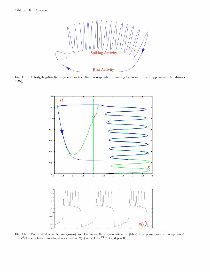
1254 E. M. Izhikevich
Rest Activity
Spiking Activity
Fig. 113. A hedgehog-like limit cycle attractor often corresponds to bursting behavior (from [Hoppensteadt & Izhikevich,1997]).
2 1.5 1 0.5 0 0.5 1 1.5 2 2.5 31
0.8
0.6
0.4
0.2
0
0.2
0.4
0 50 100 150 200 250 300 350 400 4502
1.5
1
0.5
0
0.5
1
1.5
2
2.5
3
x(t)
x
u
Fig. 114. Fast and slow nullclines (green) and Hedgehog limit cycle attractor (blue) in a planar relaxation system x =x− x3/3− u+ 4S(x) cos 40u, u = µx, where S(x) = 1/(1 + e5(1−x)) and µ = 0.01.

Neural Excitability, Spiking and Bursting 1255
2.5
2
1.5
1
0.5
0
0.5
1.51
0.5
0
0.5
1
0.4
0.2
0
0.2
0.4
0 20 40 60 80 100 120 1402.5
2
1.5
1
0.5
0
0.5
y(t)
x
y
z
"Blue-Sky" Bursting
Rest
Spiking
Fig. 115. Hedgehog bursting of the “Blue-sky” type. Simulations of the Gavrilov–Shilnikov model [Kuznetsov, 1995, p. 256].Parameters: b = 10, ε = 0.02, µ = 0.5.
Single Spike Doublet Burst of Spikes
Fig. 116. Secondary homoclinic orbits to saddle–focus equilibrium can bifurcate into periodic solutions corresponding todoublets, triplets (not shown) or bursts of spikes.

1256 E. M. Izhikevich
Fig. 117. An example of a quasiperiodic signal. x(t) = sin ω1t sin ω2t with the frequency vector (ω1, ω2) = (1,√
2/20).
"Homoclinic Torus" Bursting
Fig. 118. “Homoclinic torus” bursting. The pattern depends on the location of the disappeared fold limit cycle (dotted bluecircle).

Neural Excitability, Spiking and Bursting 1257
0 5 10 15 20 25 30 3520
15
10
5
0
5
10
15
20
x(t)
Fig. 119. Solution of the Lorenz system resembles chaotic cycle–cycle bursting.
32
10
12
3 3
2
1
0
1
2
3
3
2
1
0
1
2
3
x
u
u
0 50 100 150 200 250 300 350 400 4503
2
1
0
1
2
3
x(t)
x
Fig. 120. Chaotic bursting near saddle–focus homoclinic orbit bifurcation. Simulations of a system x = x−x3/3 + I − Reu,u = µ(S(x)(1 + ωi)u− u/2), where u ∈ C, S(x) = 1/(1 + e−5x), ω = −10, I = 0.75, µ = 0.1.

1258 E. M. Izhikevich
chaotic bursting. Terman’s arguments can begeneralized to most “*/homoclinic” bursters.
6. Classification of Bursters:Why Bother?
There are many types of distinct bursters from thepurely dynamical system point of view. Are they re-ally so different from the neuro-computational pointof view? The answer is maybe.
Indeed, some bursters have quite unique neuro-computational properties. For example, the“circle/circle” (“parabolic”) bursting exhibits Class1 neural excitability and Class 1 spiking, and it mayact as an integrator of neural signals when it oc-curs via “fold/*” hysteresis loop. In contrast, the“subHopf/fold cycle” (“elliptic”) burster exhibitsClass 2 neural excitability and Class 2 spiking,and it acts as a resonator. Interactions betweensuch resonator bursters depend crucially on the res-onant relations between their interspike frequen-cies [Izhikevich, 2000a]; they can exhibit spike syn-chronization, burst synchronization, or both. Incontrast, “circle/circle” bursters do not have well-defined interspike frequencies, and hence are reluc-tant to exhibit spike synchronization.
Thus, different bursters can communicate, syn-chronize, and process information differently. How-ever, we cannot exclude the case when a pair ofdistinct bursters has identical neuro-computationalproperties, since there are so many bursters [seeTable 4], and so little information about theirbehavior.
6.1. How to distinguish bursters?
Since different bursters may have different neuro-computational properties, it is important to havecriteria to distinguish them experimentally. Theleast useful, but probably the most common way,is to browse through this paper and try to finda picture that “resembles” micro-electrode record-ings under consideration. This might be a com-plete waste of time since two identical bursters maylook quite different (Fig. 121) or two quite dis-tinct bursters may look “similar”; compare “cir-cle/circle” bursting in Fig. 57 and “fold/big homo-clinic” bursting in Fig. 86.
6.1.1. Frequency of emerging/terminating spiking
First, one should inspect the frequency of emerg-ing and terminating spiking and compare it with
C
hR2
Fig. 121. Two topologically equivalent (via homeomorphismh) “subHopf/fold cycle” bursters may “look” quite different(from [Izhikevich, 2000a]).
the interspike frequency in the middle of a burst.A significant drop of the frequency is a good in-dicator of saddle–node on invariant circle and sad-dle homoclinic orbit bifurcations. For example, ifwe consider the planar case, then small initial fre-quency implies “circle/*” bursting. Similarly, smallterminating frequency implies “*/circle” or “*/ho-moclinic” bursting. If there is no significant changein the frequency during the burst, then possible bi-furcations are of fold or Andronov–Hopf type; seeTables 1 and 2.
Guckenheimer et al. [1997] used heuristic ar-guments and obtained detailed asymptotics of theinterspike frequency at the end of the burst, whichcould be used to distinguish, e.g. “*/circle” from“*/homoclinic” bursting.
6.1.2. Amplitude of emerging/terminating spiking
A small amplitude initial or terminating spiking is astrong indicator against fold, saddle–node on invari-ant circle, and saddle homoclinic orbit bifurcations,since it occurs only during Andronov–Hopf and foldlimit cycle bifurcations. However, large amplitudespiking cannot rule out Andronov–Hopf and foldlimit cycle bifurcations, since many relaxation sys-tems near (singular) Andronov–Hopf bifurcationsexhibit small and intermediate amplitude spikingonly in an extremely narrow region of bifurcationparameters; see e.g. Figs. 73 and 76.
6.1.3. Damped oscillations at rest
Existence of damped subthreshold oscillation is astrong indicator of nearness to an Andronov–Hopf

Neural Excitability, Spiking and Bursting 1259
ThresholdManifold
Node-Focus
Saddle-Focus
Fig. 122. A small perturbation may exhibit damped os-cillation even though the system is near fold bifurcationpoint.
bifurcation. Its frequency is the neuron’s resonantfrequency. However, damped oscillations may existeven for fold bifurcation provided that the dimen-sion of the system is greater than 2; see Fig. 122.
Such an oscillation does not make the neurona resonator, since it occurs in a subspace tangentto the stable manifold of the saddle–node. Increas-
ing the amplitude of the oscillation does not changesignificantly the distance to the threshold manifold,and hence does not facilitate the spike.
6.1.4. Spike undershoot
Can the presence or lack of spike undershoot beused to distinguish different types of bursters? Theanswer is NO.
It is commonly believed that the undershootoccurs because the limit cycle attractor correspond-ing to the repetitive spiking encompasses the equi-librium corresponding to the quiescent state. Thisindeed leads to the undershoot, but only in a two-dimensional fast subsystem. Moreover, the under-shoot may occur without the encompassing, as weillustrate in Fig. 123. This suggests, in particu-lar, that the famous “fold/homoclinic” (“square-wave” or “Type Ia”) bursting may display under-shoot even when the fast subsystem is planar.
If the fast system is multidimensional, thenwhether the limit cycle surrounds the equilibrium
v
v v v v v
v
v(t)
v
v v v v v
v
v(t)
Fold Bifurcation Saddle HomoclinicOrbit Bifurcation
No SpikeUndershoot
"Fold/Homoclinic" ("Square-Wave") Bursting
SpikeUndershoot
Fold Bifurcation Saddle HomoclinicOrbit Bifurcation
Fig. 123. Spike undershoot in “fold/homoclinic” (“square-wave” or “Type Ia”) bursting.
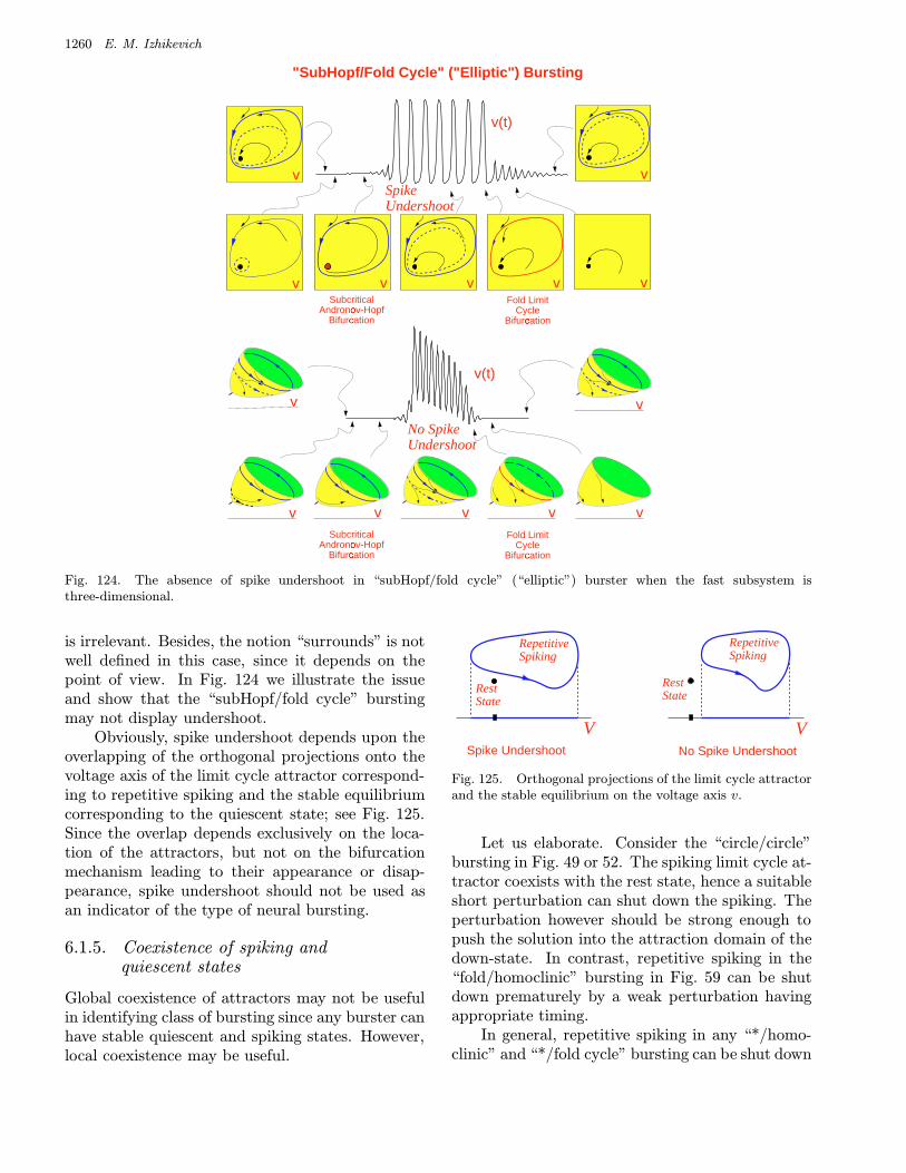
1260 E. M. Izhikevich
v
SubcriticalAndronov-Hopf
Bifurcation
Fold LimitCycle
Bifurcation
v(t)
v v v v v
v
"SubHopf/Fold Cycle" ("Elliptic") Bursting
v
v v v v v
vSpikeUndershoot
v(t)
SubcriticalAndronov-Hopf
Bifurcation
Fold LimitCycle
Bifurcation
No SpikeUndershoot
Fig. 124. The absence of spike undershoot in “subHopf/fold cycle” (“elliptic”) burster when the fast subsystem isthree-dimensional.
is irrelevant. Besides, the notion “surrounds” is notwell defined in this case, since it depends on thepoint of view. In Fig. 124 we illustrate the issueand show that the “subHopf/fold cycle” burstingmay not display undershoot.
Obviously, spike undershoot depends upon theoverlapping of the orthogonal projections onto thevoltage axis of the limit cycle attractor correspond-ing to repetitive spiking and the stable equilibriumcorresponding to the quiescent state; see Fig. 125.Since the overlap depends exclusively on the loca-tion of the attractors, but not on the bifurcationmechanism leading to their appearance or disap-pearance, spike undershoot should not be used asan indicator of the type of neural bursting.
6.1.5. Coexistence of spiking andquiescent states
Global coexistence of attractors may not be usefulin identifying class of bursting since any burster canhave stable quiescent and spiking states. However,local coexistence may be useful.
V V
RestState
RepetitiveSpiking
RestState
RepetitiveSpiking
Spike Undershoot No Spike Undershoot
Fig. 125. Orthogonal projections of the limit cycle attractorand the stable equilibrium on the voltage axis v.
Let us elaborate. Consider the “circle/circle”bursting in Fig. 49 or 52. The spiking limit cycle at-tractor coexists with the rest state, hence a suitableshort perturbation can shut down the spiking. Theperturbation however should be strong enough topush the solution into the attraction domain of thedown-state. In contrast, repetitive spiking in the“fold/homoclinic” bursting in Fig. 59 can be shutdown prematurely by a weak perturbation havingappropriate timing.
In general, repetitive spiking in any “*/homo-clinic” and “*/fold cycle” bursting can be shut down

Neural Excitability, Spiking and Bursting 1261
prematurely by a weak stimulation, while that in“*/circle” and “*/Hopf” cannot. Similarly, a briefweak stimulation can evoke repetitive spiking in“fold/*” and “subHopf/*” bursters, and cannot in“circle/*” and “Hopf/*” bursters.
Finally, notice that testing for coexistenceof attractors is an invasive procedure that re-quires stimulation, while the other criteria discussedabove are noninvasive because they are based onlyon observations.
6.1.6. Transition from bursting to tonicspiking or quiescence
Fine structure of a bursting pattern depends onmany physiological parameters, such as temper-ature, concentration of extracellular ions, etc.Changing such parameters can distort the burst-ing pattern, and in extreme cases, can shut it downcompletely or transform it to a tonic spiking. Theseare interesting cases because they correspond to abifurcation in the behavior of the entire system.Measuring the interspike and/or interburst inter-vals at the bifurcation, one can in principle deter-mine the type of bursting the system can exhibit.Unfortunately, little is known about possible mech-anisms of transition from bursting to tonic spikingor quiescence, except in some special cases discussedby Terman [1992] and Izhikevich [2000a]. Thus,more analysis is needed before one can make senseof those measurements.
6.1.7. Conductance based models
We have treated neurons as general dynamical sys-tems with no restriction on the form of the right-hand side. Now we restrict ourselves and considerthe conductance-based models of the form
V = I −n∑i=1
gi(x)(V −Ei)
x = f(V, x)
where V is the voltage, and x ∈ Rm is the vector ofconductances, gating variables, etc. Does the con-ductance based form impose any restriction on thepossible bifurcations of the rest state or limit cycle?Could some bifurcation always lead to spike un-dershoot or overshoot? These are important openproblems.
7. Conclusion
In this paper we review relevant bifurcations thatare involved in the generation of action poten-tials by neurons. The bifurcations determine ex-citable properties of neurons, and hence their neuro-computational features, which are summarized inTables 1 and 2. Table 4 classifies fast–slow bursters.Among them only a few, shown in Fig. 126, wereidentified before, the others are new.
Neurons: Integrators or resonators? The typeof bifurcation of the rest state determines the mostimportant neuro-computational feature of the neu-ron: It is either an integrator or a resonator.
• Integrator. If the rest state disappears via foldor saddle–node on invariant circle bifurcations,then the neuron acts as an integrator; the higherthe frequency of the input, the sooner it fires.• Resonator. If the rest state disappears via an
Andronov–Hopf bifurcation, then the neuron actsas a resonator; it prefers a certain (resonant) fre-quency of the input spike train that is equal to alow-order multiple of its eigenfrequency. Increas-ing the frequency of the input may delay or eventerminate its response.
Integrators have a well-defined threshold man-ifold, while resonators usually do not. Integratorsdistinguish between weak excitatory and inhibitoryinputs, while resonators do not, since an inhibitorypulse can make a resonator fire. Integrators caneasily encode information about the intensity ofstimulation into their mean firing rate, whereas res-onators cannot. In contrast, resonators are sensi-tive to the fine temporal structure of the input spiketrain, while integrators are not because they average(integrate) it. It is curious that many investigatorstried to illustrate various aspects of sensitivity ofbiological neurons to timings of spikes, such as coin-cidence detection, using only the integrate-and-firemodel.
Another astonishing fact is that many neuro-computational features of integrators, such as all-or-none response and threshold manifold, havebeen introduced by studying the classical Hodgkin–Huxley model, which is a resonator, and hence doeshave these features.
Bursting. All bursting neurons seem to havesimilar behavior: Repetitive spiking, then quies-cence, then spiking again, and so on. However,
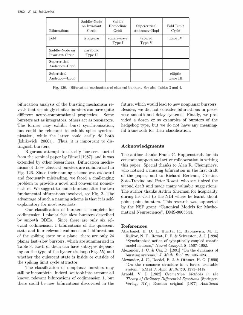
1262 E. M. Izhikevich
Saddle–Node Saddleon Invariant Homoclinic Supercritical Fold Limit
Bifurcations Circle Orbit Andronov–Hopf Cycle
Fold triangular square-wave tapered Type IV
Type I Type V
Saddle–Node on parabolic
Invariant Circle Type II
Supercritical
Andronov–Hopf
Subcritical elliptic
Andronov–Hopf Type III
Fig. 126. Bifurcation mechanisms of classical bursters. See also Tables 3 and 4.
bifurcation analysis of the bursting mechanism re-veals that seemingly similar bursters can have quitedifferent neuro-computational properties. Somebursters act as integrators, others act as resonators.The former may exhibit burst synchronization,but could be reluctant to exhibit spike synchro-nization, while the latter could easily do both[Izhikevich, 2000a]. Thus, it is important to dis-tinguish bursters.
Rigorous attempt to classify bursters startedfrom the seminal paper by Rinzel [1987], and it wasextended by other researchers. Bifurcation mecha-nisms of those classical bursters are summarized inFig. 126. Since their naming scheme was awkwardand frequently misleading, we faced a challengingproblem to provide a novel and convenient nomen-clature. We suggest to name bursters after the twofundamental bifurcations involved, see Fig. 2. Theadvantage of such a naming scheme is that it is self-explanatory for most scientists.
Our classification of bursters is complete forcodimension 1 planar fast–slow bursters describedby smooth ODEs. Since there are only six rel-evant codimension 1 bifurcations of the quiescentstate and four relevant codimension 1 bifurcationsof the spiking state on a plane, there are only 24planar fast–slow bursters, which are summarized inTable 3. Each of them can have subtypes depend-ing on the type of the hysteresis loop (Fig. 55) andwhether the quiescent state is inside or outside ofthe spiking limit cycle attractor.
The classification of nonplanar bursters maystill be incomplete. Indeed, we took into account allknown relevant bifurcations of codimension 1, butthere could be new bifurcations discovered in the
future, which would lead to new nonplanar bursters.Besides, we did not consider bifurcations in piece-wise smooth and delay systems. Finally, we pro-vided a dozen or so examples of bursters of thehedgehog type, but we do not have any meaning-ful framework for their classification.
Acknowledgments
The author thanks Frank C. Hoppensteadt for hisconstant support and active collaboration in writingthis paper. Special thanks to Alan R. Champneys,who noticed a missing bifurcation in the first draftof the paper, and to Richard Bertram, CristinaSoto-Trevino and Peter Rowat, who scrutinized thesecond draft and made many valuable suggestions.The author thanks Arthur Sherman for hospitalityduring his visit to the NIH where he learnt aboutpoint–point bursters. This research was supportedby the NSF grant “Canonical Models for Mathe-matical Neuroscience”, DMS-9805544.
ReferencesAbarbanel, H. D. I., Huerta, R., Rabinovich, M. I.,
Rulkov, N. F., Rowat, P. F. & Selverston, A. I. [1996]“Synchronized action of synaptically coupled chaoticmodel neurons,” Neural Comput. 8, 1567–1602.
Alexander, J. C. & Cai, D. [1991] “On the dynamics ofbursting systems,” J. Math. Biol. 29, 405–423.
Alexander, J. C., Doedel, E. J. & Othmer, H. G. [1990]“On the resonance structure in a forced excitablesystem,” SIAM J. Appl. Math. 50, 1373–1418.
Arnold, V. I. [1982] Geometrical Methods in theTheory of Ordinary Differential Equations (Springer-Verlag, NY); Russian original [1977] Additional
Neural Excitability, Spiking and Bursting 1263
Chapters of the Theory of Ordinary DifferentialEquations, Moscow.
Arnold, V. I., Afrajmovich, V. S., Il’yashenko, Yu. S. &Shil’nikov, L. P. [1994] “Bifurcation theory,” in Dy-namical Systems V. Bifurcation Theory and Catastro-phe Theory, ed. Arnold, V. I. (Springer-Verlag, NY).
Aronson, D. G., Ermentrout, G. B. & Kopell, N. [1990]“Amplitude response of coupled oscillators,” PhysicaD41, 403–449.
Baer, S. M., Erneux, T. & Rinzel, J. [1989] “The slowpassage through a Hopf bifurcation: Delay, memoryeffects, and resonances,” SIAM J. Appl. Math. 49,55–71.
Baer, S. M., Rinzel, J. & Carrillo, H. [1995] “Analysisof an autonomous phase model for neuronal parabolicbursting,” J. Math. Biol. 33, 309–333.
Bedrov, Y. A., Akoev, G. N. & Dick, O. E. [1992] “Par-tition of the Hodgkin–Huxley type model parameterspace into regions of qualitatively different solutions,”Biol. Cybern. 66, 413–418.
Belair, J. & Holmes, P. [1984] “On linearly coupled re-laxation oscillations,” Quarterly of Appl. Math. 42,193–219.
Bertram, R. [1993] “A computational study of the effectsof serotonin on a molluscan burster neuron,” Biol.Cybern. 69, 257–267.
Bertram, R., Butte, M. J., Kiemel, T. & Sherman, A.[1995] “Topological and phenomenological classifica-tion of bursting oscillations,” Bull. Math. Biol. 57,413–439.
Booth, V., Carr, T. W. & Erneux, T. [1997] “Near-threshold bursting is delayed by a slow passage neara limit point,” SIAM J. Appl. Math. 57, 1406–1420.
Butera Jr., R. J., Clark Jr., J. W. & Byrne, J. H. [1996]“Dissection and reduction of a modeled burstingneuron,” J. Comput. Neurosci. 3, 199–223.
Butera Jr., R. J., Clark Jr., J. W. & Byrne, J. H. [1997]“Transient responses of a modeled bursting neuron:Analysis with equilibrium and averaged nullclines,”Biol. Cybern. 77, 307–322.
Canavier, C. C., Clark, J. W. & Byrne, J. H. [1991]“Simulation of the bursting activity of neuron-R15in aplysia — role of ionic currents, calcium balance,and modulatory transmitters,” J. Neurophysiol. 66,2107–2124.
Carpenter, G. A. [1979] “Bursting phenomena in ex-citable membranes,” SIAM J. Appl. Math. 36,334–372.
Chay, T. R. & Keizer, J. [1983] “Minimal model for mem-brane oscillations in the pancreatic β-cell,” Biophys.J. 42, 181–190.
Connor, J. A. & Stevens, C. F. [1971] “Prediction ofrepetitive firing behavior from voltage-clamped dataon an isolated neurone soma,” J. Physiol. Lond. 214,31–53.
Del Negro, C. A., Hsiao, C.-F., Chandler, S. H. &
Garfinkel, A. [1998] “Evidence for novel burstingmechanism in rodent trigeminal neurons,” Biophys. J.75, 174–182.
de Vries, G. [1998] “Multiple bifurcations in a polyno-mial model of bursting oscillations,” J. Nonlin. Sci.8, 281–316.
Ermentrout, G. B. [1996] “Type I membranes, phaseresetting curves, and synchrony,” Neural Comput. 8,979–1001.
Ermentrout, G. B. [1998] “Linearization of F-I curves byadaptation,” Neural Comput. 10, 1721–1729.
Ermentrout, G. B. & Kopell, N. [1986a] “Parabolic burst-ing in an excitable system coupled with a slow oscil-lation,” SIAM J. Appl. Math. 46, 233–253.
Ermentrout, G. B. & Kopell, N. [1986b] “Subcellular os-cillations and bursting,” Math. Biosci. 78, 265–291.
Evans, J., Fenichel, N. & Feroe, J. [1982] “Double im-pulse solutions in nerve axon equations,” SIAM J.Appl. Math. 42, 219–234.
Fenichel, N. [1971] “Persistence and smoothness of in-variant manifolds for flows,” Ind. Univ. Math. J. 21,193–225.
Feroe, J. A. [1982] “Existence and stability of multipleimpulse solutions of a nerve equation,” SIAM J. Appl.Math. 42, 235–246.
FitzHugh, R. [1955] “Mathematical models of thresh-old phenomena in the nerve membrane,” Bull. Math.Biophys. 17, 257–278.
Frankel, P. & Kiemel, T. [1993] “Relative phase behav-ior of two slowly coupled oscillators,” SIAM J. Appl.Math. 53, 1436–1446.
Grasman, J. [1987] Asymptotic Methods for RelaxationOscillations and Applications (Springer-Verlag, NY).
Guckenheimer, J., Harris-Warrick, R., Peck, J. &Willms, A. [1997] “Bifurcations, bursting and spikefrequency adaptation,” J. Comput. Neurosci. 4,257–277.
Gutfreund, Y., Yarom, Y. & Segev, I. [1995] “Subthresh-old oscillations and resonant frequency in guinea-pigcortical neurons: Physiology and modeling,” J. Phys-iol. London 483, 621–640.
Gutkin, B. S. & Ermentrout, G. B. [1998] “Dynam-ics of membrane excitability determine interspike in-terval variability: A link between spike generationmechanisms and cortical spike train statistics,” NeuralComput. 10, 1047–1065.
Hansel, D., Mato, G. & Meunier, C. [1995] “Synchronyin excitatory neural networks,” Neural Comput. 7,307–335.
Hassard, B. D. [1978] “Bifurcation of periodic solutionsof the Hodgkin–Huxley model for the squid giantaxon,” J. Theoret. Biol. 71, 401–420.
Hassard, B. D., Kazarinoff, N. D. & Wan, Y. H. [1981]Theory and Applications of Hopf Bifurcation (Cam-bridge University Press, Cambridge).
Hastings, S. [1976] “On the existence of homoclinic

1264 E. M. Izhikevich
and periodic orbits for FitzHugh–Nagumo equations,”Quart. J. Math. (Oxford) 27, 123–134.
Hindmarsh, J. L. & Rose, R. M. [1984] “A model of neu-ronal bursting using three coupled first order differen-tial equations,” Philos. Trans. R. Soc. London, Ser.B221 87–102.
Hodgkin, A. L. [1948] “The local electric changes associ-ated with repetitive action in a non-medulated axon,”J. Physiol. 107, 165–181.
Hodgkin, A. L. & Huxley, A. F. [1952] “A quantitativedescription of membrane current and application toconduction and excitation in nerve,” J. Physiol. 117,500–544.
Holden, L. & Erneux, T. [1993a] “Slow passage througha Hopf bifurcation: Form oscillatory to steady statesolutions,” SIAM J. Appl. Math. 53, 1045–1058.
Holden, L. & Erneux, T. [1993b] “Understanding burst-ing oscillations as periodic slow passages throughbifurcation and limit points,” J. Math. Biol. 31,351–365.
Holden, A. V., Hyde, J. & Muhamad, M. [1991] “Equi-libria. Periodicity, bursting and chaos in neural activ-ity,” Proc. 9th Summer Workshop on MathematicalPhysics, Vol. 1, pp. 96–128.
Hoppensteadt, F. C. [1997] An Introduction to theMathematics of Neurons. Modeling in the FrequencyDomain (Cambridge University Press).
Hoppensteadt, F. C. [1993] Analysis and Simulations ofChaotic Systems (Springer-Verlag, NY).
Hoppensteadt, F. C. & Izhikevich, E. M. [1996] “Synap-tic organizations and dynamical properties of weaklyconnected neural oscillators: I. Analysis of canonicalmodel,” Biol. Cybern. 75, 117–127.
Hoppensteadt, F. C. & Izhikevich, E. M. [1997] WeaklyConnected Neural Networks (Springer-Verlag, NY).
Hoppensteadt, F. C. & Izhikevich, E. M. [1998]“Thalamo-Cortical interactions modeled by weaklyconnected oscillators: Could brain use FM radioprinciples?” BioSyst. 48, 85–94.
Hutcheon, B., Miura, R. M. & Puil, E. [1996] “Mod-els of subthreshold membrane resonance in neocorticalneurons,” J. Neurophysiol. 76, 698–714.
Hutcheon, B., Miura, R. M., Yarom, Y. & Puil, E. [1994]Low-threshold calcium current and resonance in tha-lamic neurons: A model of frequency preference,” J.Neurophysiol. 71, 583–594.
Il’iashenko, Iu. S. & Li, W. [1999] Nonlocal Bifurca-tions Mathematical Surveys and Monographs (Amer-ican Mathematical Society), Vol. 66.
Izhikevich, E. M. [2001] “Resonate-and-fire neurons,”Neural Networks, submitted.
Izhikevich, E. M. [2000a] “Subcritical elliptic bursting ofBautin type,” SIAM J. Appl. Math. 60, 503–535.
Izhikevich, E. M. [2000b] “Phase equations for relaxationoscillators,” SIAM J. Appl. Math., in press.
Izhikevich, E. M. [1999a] “Weakly connected quasiperi-
odic oscillators, FM interactions, and multiplexing inthe brain,” SIAM J. Appl. Math. 59, 2193–2223.
Izhikevich, E. M. [1999b] “Class 1 neural excitability,conventional synapses, weakly connected networks,and mathematical foundations of pulse-coupled mod-els,” IEEE Trans. Neural Networks 10, 499–507.
Izhikevich, E. M. [1999c] “Weakly pulse-coupled oscilla-tors, FM interactions, synchronization, and oscillatoryassociative memory,” IEEE Trans. Neural Networks10, 508–526.
Izhikevich, E. M. [1998] “Supercritical elliptic bursting,slow passage effect, and assistance of noise,” preprint.
Jansen, H. & Karnup, S. [1994] “A spectral analysisof the integration of artificial synaptic potentials inmammalian central neurons,” Brain Res. 666, 9–20.
Johnston, D. & Wu, S. M. [1995] Foundations of CellularNeurophysiology (The MIT Press).
Kopell, N. [1995] “Chains of coupled oscillators,” inBrain Theory and Neural Networks, ed. Arbib, M. A.(The MIT press, Cambridge, MA).
Kopell, N. & Somers, D. [1995] “Anti-phase solutions inrelaxation oscillators coupled through excitatory in-teractions,” J. Math. Biol. 33, 261–280.
Kowalski, J. M., Albert, G. L., Rhoades, B. K. & Gross,G. W. [1992] “Neuronal networks with spontaneous,correlated bursting activity: Theory and simulations,”Neural Networks 5, 805–822.
Kuznetsov, Yu. [1995] Elements of Applied BifurcationTheory 2nd edition (Springer-Verlag, NY).
Levi, M., Hoppensteadt, F. C. & Miranker, W. L. [1978]“Dynamics of the Josephson junction,” Quart. J.Appl. Math. July, 167–190.
Llinas, R. R. [1988] “The intrinsic electrophysio-logical properties of mammalian neurons: Insightsinto central nervous system function,” Science 242,1654–1664.
Llinas, R. R., Grace, A. A. & Yarom, Y. [1991] “In vitroneurons in mammalian cortical layer 4 exhibit intrin-sic oscillatory activity in the 10- to 50-Hz frequencyrange,” Proc. Natl. Acad. Sci. USA 88, 897–901.
Mishchenko, E. F., Kolesov, Yu. S., Kolesov, A. Yu. &Rozov, N. K. [1994] Asymptotic Methods in SingularlyPerturbed Systems (Plenum Press, NY).
Morris, C. & Lecar, H. [1981] “Voltage oscillations in theBarnacle giant muscle fiber,” Biophys. J. 35, 193–213.
Nejshtadt, A. [1985] “Asymptotic investigation of theloss of stability by an equilibrium as a pair of eigenval-ues slowly cross the imaginary axis,” Usp. Mat. Nauk40, 190–191.
Pernarowski, M. [1994] “Fast subsystem bifurcations ina slowly varied Lienard system exhibiting bursting,”SIAM J. Appl. Math. 54, 814–832.
Pernarowski, M., Miura, R. M. & Kevorkian, J. [1992]“Perturbation techniques for models of bursting elec-trical activity in pancreatic β-cells,” SIAM J. Appl.Math. 52, 1627–1650.

Neural Excitability, Spiking and Bursting 1265
Plant, R. E. [1981] “Bifurcation and resonance in a modelfor bursting nerve cells,” J. Math. Biol. 11, 15–32.
Puil, E., Meiri, H., Yarom, Y. [1994] “Resonant behav-ior and frequency preference of thalamic neurons,” J.Neurophysiol. 71, 575–582.
Rinzel, J. [1987] “A formal classification of burstingmechanisms in excitable systems,” Mathematical Top-ics in Population Biology, Morphogenesis, and Neuro-sciences, eds. Teramoto, E. & Yamaguti, M., Vol. 71of Lecture Notes in Biomathematics (Springer-Verlag,Berlin).
Rinzel, J. & Ermentrout, G. B. [1989] “Analysis of neuralexcitability and oscillations,” eds. Koch, C. & Segev,I. Methods in Neuronal Modeling (The MIT Press,Cambridge).
Rinzel, J. & Lee, Y. S. [1986] “On different mechanismsfor membrane potential bursting,” Nonlinear Oscilla-tions in Biology and Chemistry, ed. Othmer, H. G.,Lecture Notes in Biomathematics (Springer-Verlag).
Rinzel, J. & Lee, Y. S. [1987] “Dissection of a modelfor neuronal parabolic bursting,” J. Math. Biol. 25,653–675.
Rinzel, J. & Miller, R. N. [1980] “Numerical calcula-tion of stable and unstable periodic solution to theHodgkin–Huxley equations,” Math. Biosci. 49, 27–59.
Rush, M. E. & Rinzel, J. [1995] “The potassium A-Current, low firing rates and rebound excitationin Hodgkin–Huxley models,” Bull. Math. Biol. 57,899–929.
Rush, M. E. & Rinzel, J. [1994] “Analysis of bursting ina thalamic neuron model,” Biol. Cybern. 71, 281–291.
Samoilenko, A. M. [1991] “Elements of the mathematicaltheory of multi-frequency oscillations,” Mathematicsand Its Applications (Soviet Series), Vol. 71 (KluwerAcademic, Dordrecht).
Schecter, S. [1987] “The saddle-node separatrix-loop bi-furcation,” SIAM J. Math. Anal. 18, 1142–1156.
Sharp, A. A., O’neil, M. B., Abbott, L. F. & Marder, E.[1993] “Dynamic clamp: Computer-generated conduc-tances in real neurons,” J. Neurophysiol. 69, 992–995.
Shepherd, G. M. [1981] “Introduction: The nerve impulseand the nature of nervous function,” Neurones With-out Impulses, eds. Roberts & Bush (Cambridge Uni-versity Press).
Shepherd, G. M. [1983] Neurobiology (Oxford UniversityPress, NY).
Shorten, P. R. & Wall, D. J. N. [2000] “A Hodgkin–Huxley model exhibiting bursting oscillations,” Bull.Math. Biol., accepted.
Sivan, E., Segel, L. & Parnas, H. [1995] “Modulated ex-citability: A new way to obtain bursting neurons,”Biol. Cybern. 72, 455–461.
Smolen, P., Terman, D. & Rinzel, J. [1993] “Properties ofa bursting model with two slow inhibitory variables,”SIAM J. Appl. Math. 53, 861–892.
Softky, W. R. & Koch, C. [1993] “The highly irregu-
lar firing of cortical-cells is inconsistent with tempo-ral integration of random EPSPs,” J. Neurosci. 13,334–350.
Somers, D. & Kopell, N. [1993] “Rapid synchronizationthrough fast threshold modulation,” Biol. Cybern. 68,393–407.
Somers, D. & Kopell, N. [1995] “Waves and synchronyin networks of oscillators or relaxation and non-relaxation type,” Physica D89, 169–183.
Soto-Trevino, C., Kopell, N. & Watson, D. [1996]“Parabolic bursting revisited,” J. Math. Biol. 35,114–128.
Storti, D. W. & Rand, R. H. [1986] “Dynamics oftwo strongly coupled relaxation oscillators,” SIAM J.Appl. Math. 46, 56–67.
Taylor, D. & Holmes, P. [1998] “Simple models for ex-citable and oscillatory neural networks,” J. Math.Biol. 37, 419–446.
Terman, D. [1991] “Chaotic spikes arising from a modelof bursting in excitable membranes,” SIAM J. Appl.Math. 51, 1418–1450.
Terman, D. [1992] “The transition from bursting to con-tinuous spiking in excitable membrane models,” J.Nonlinear Sci. 2, 133–182.
Terman, D. & Lee, E. [1997] “Partial synchronization ina network of neural oscillators,” SIAM J. Appl. Math.57, 252–293.
Terman, D. & Wang, D. [1995] “Global competition andlocal cooperation in a network of neural oscillators,”Physica D81, 148–176.
Traub, R. D. & Miles, R. [1991] Neuronal Networksof the Hippocampus (Cambridge University Press,Cambridge).
Troy, W. [1978] “The bifurcation of periodic solutions inthe Hodgkin–Huxley equations,” Quart. Appl. Math.36, 73–83.
Wang, X.-J. [1993] “Ionic basis for intrinsic 40 Hz neu-ronal oscillations,” NeuroReport 5, 221–224.
Wang, X.-J. [1993] “Genesis of bursting oscillations inthe Hindmarsh–Rose model and homoclinicity to achaotic saddle,” Physica D62, 263–274.
Wang, X.-J. [1998] “Calcium coding and adaptive tem-poral computation in cortical pyramidal neurons,” J.Neurophysiol. 79, 1549–1566.
Wang, X. J. & Rinzel, J. [1995] “Oscillatory and burstingproperties of neurons,” Brain Theory and Neural Net-works, ed. Arbib, M. A. (The MIT press, Cambridge,MA).
Williams, T. L. & Sigvardt, K. A. [1995] “Spinal cordof lamprey: Generation of locomotor patterns,” BrainTheory and Neural Networks, ed. Arbib, M.A. (TheMIT press, Cambridge, MA).
Wilson, C. J. [1993] “The generation of natural firingpatterns in neostriatal neurons,” Progress in BrainResearch, eds. Arbuthnott, G. W. & Emson, P. C. 99,pp. 277–297.
1266 E. M. Izhikevich
Wilson, C. J. & Kawaguchi, Y. [1996] “The origins oftwo-state spontaneous membrane potential fluctua-tions of neostriatal spiny neurons,” J. Neurosci. 16,2397–2410.
Wilson, H. R. & Cowan, J. D. [1972] “Excitatory and in-hibitory interaction in localized populations of modelneurons,” Biophys J. 12, 1–24.
Wilson, M. A. & Bower, J. M. [1989] “The simulationof large scale neural networks,” Methods in NeuronalModeling, eds. Koch, C. & Segev, I. (The MIT Press,Cambridge, MA).
Wu, H.-Y. & Baer, S. M. [1998] “Analysis of an excitabledendritic spine with an activity-dependent stemconductance,” J. Math. Biol. 36, 569–592.