Networking Unleashed: Geographic Routing and ... - ETH Z · DISS. ETH NO. 16025 Networking Unleashed: Geographic Routing and Topology Control in Ad Hoc and Sensor Networks A dissertation

DISS. ETH NO. 16025

Networking Unleashed:

Geographic Routing and Topology Control

in Ad Hoc and Sensor Networks

A dissertation submitted to the

SWISS FEDERAL INSTITUTE OF TECHNOLOGY ZURICH

for the degree of

Doctor of Sciences

presented by

AARON ZOLLINGER

Dipl. Inf.-Ing., ETH Zurich

born 24.04.1975

citizen of

Zurich ZH and Regensdorf ZH

accepted on the recommendation of

Prof. Dr. Roger Wattenhofer, examiner

Prof. Dr. Matthias Grossglauser, co-examiner

Charles E. Perkins, co-examiner

2005

Abstract

Ad hoc and sensor networks consist of autonomous devices communicatingvia radio equipment. Common scenarios for ad hoc networks include surviv-able, efficient, dynamic communication networks for emergency and rescue op-erations, disaster relief efforts, and similar tasks where typically no communica-tion infrastructure is present prior to the deployment of the ad hoc network. Insensor networks, nodes are additionally equipped with sensors, performing thetask of sensing a certain physical value, such as temperature, humidity, bright-ness, or motion, and periodically reporting the sensed data to a designated sinknode for monitoring purposes.

Since ad hoc and sensor network nodes are generally assumed to be au-tonomous and operate for a considerable period of time—in case of sensor net-works up to several years—, energy conservation is one of the central issues inthis research context. On the other hand, many scenarios assume a high degreeof dynamics, particularly based on node mobility.

This dissertation discusses two major problem fields in the context of ad hocand sensor networks. In particular, geographic routing—a local type of routinginherently well suited for dynamic ad hoc networks—is studied with respectto both worst-case and average-case networks. Second, topology control basedon transmission power reduction puts the focus on energy conservation as aconsequence of restricted interference among the network nodes.

Zusammenfassung

Ad-Hoc- und Sensornetze bestehen aus unabhangigen uber Funk kommuni-zierenden Geraten. Haufig genannte Szenarien fur Ad-Hoc-Netzwerke beschrei-ben ihren Einsatz als robuste, sparsame und dynamische Kommunikationsnetzefur Notfall- und Rettungseinsatze, Katastrophenhilfe und ahnliche Aufgaben,wo vor dem Einsatz des Ad-Hoc-Netzwerkes keine Kommunikationsinfrastruk-tur vorhanden ist. In Sensornetzen sind die Netzwerkknoten zusatzlich mitSensoren ausgestattet, die bestimmte physikalische Grossen – wie beispielswei-se Temperatur, Feuchtigkeit, Helligkeit oder Bewegung – messen; diese Datenwerden periodisch an einen vorbezeichneten Sammelknoten gesendet und zumZwecke der Beobachtung oder der Kontrolle ausgewertet.

Da ublicherweise angenommen wird, dass Knoten in Ad-Hoc- und Sensornet-zen unabhangig von externen Energiequellen sind und trotzdem uber eine be-trachtliche Zeitspanne betrieben werden sollen – in Sensornetzen bis zu mehre-ren Jahren –, ist Energieeffizienz ein Hauptpunkt dieser Forschungsrichtung.Andererseits beinhalten viele Szenarien hohe Netzwerkdynamik, insbesondereaufgrund mobiler Knoten.

Diese Dissertation befasst sich mit zwei zentralen Problemfeldern im Be-reich von Ad-Hoc- und Sensornetzen. Im Einzelnen wird das Verhalten vongeografischem Routing – einer auf lokal begrenzter Information fussenden Artvon Nachrichtenvermittlung, die speziell gut fur den Einsatz in dynamischen Ad-Hoc-Netzwerken geeignet ist – in schlechtest moglichen und in durchschnittlichauftretenden Netzwerken untersucht. In einem zweiten Teil der Arbeit wird derSchwerpunkt auf Topologiekontrolle im Zusammenhang mit gezielt beschrankterFunksendeleistung gelegt; Energieeffizienz ist hier eine Folge von verringerterSignalstorung, oder

”Interferenz“, zwischen den Netzwerkknoten.

Acknowledgements

First of all I would like to thank my advisor Roger Wattenhofer for guidingme through the years of my PhD studies. It is true, you always took your time todiscuss any technical—or other—issues with me. It was also a very interestingand enriching experience to witness how (y)our Distributed Computing Groupgrew over the years. I hope I am worth being your first “doctoral son”.

I would also like to express my gratitude to my co-examiners Matthias Gross-glauser and Charles Perkins who both helped me improve my thesis with theirprofound and inspiring comments.

Among the most important addressees of my gratefulness are of course allmembers of the Distributed Computing Group. In particular, I would like tothank Fabian “Let’s solve a problem” Kuhn for being my patient office matefor all those years, for being my daily company, and for offering his skills tobe my hitherto most important co-author (with the exception of Roger, ofcourse); Keno “I always picture Switzerland upside-down” Albrecht for offer-ing me a German point of view on all matters discussed—by the way, Kenois the only German I know of who can enumerate all Swiss cantons with theircapitals—and for relieving me from spamania; Ruedi “I feel good!” Arnold—theonly real didact in our group—for giving me a sportive flavor of pedagogy andfor being a challenging table tennis opponent; Regina “Kvantova fizika—edinstvenna istinna nauka” O’Dell for pointing out a woman’s perspectiveon all things there are and for making fun of me on every possible and impossibleoccasion; Pascal “We’re on a highway to hell” von Rickenbach for reminding ustime and again where we all are, for his almost ubiquitous grim sense of humor,and last but not least for guiding me safely through all blizzards to my doctoralexam; Thomas “All I know, I know it from you” Moscibroda for his mastery ofmiddle names, his daily enrichment of my work hours with original word cre-ations and for behaving with due reverence; Nicolas “I will solve any problemprovided that it’s formulated correctly” Burri for being my didactic conscienceand for showing me a new perspective on human love for ruminants; Stefan “Myfavorite place was the food court” Schmid for being a pleasant companion inexploring unsought highways, hoping that you will always be able to distinguishbetween peer-to-peer and beer-to-beer; Andi “Winning to nil would be a goodidea” Wetzel for being a huge help above all during the last months with myfrequent departures and last-minute hardware and software requests; Franzi “insilico” Humair, my second unofficial office mate, for allowing me to witness thecreation of a Master thesis in biology.

Incidentally, you have all been very nice table soccer opponents; above all Iappreciate that you would let me head the ranking most of the time. You cannow stop playing therapeutically with me. . .

Of course also the work contributed by the many students I had the pleasureto assist in their theses is invaluable. I am grateful to the Diploma and Masterstudents Martin Burkhart, Pascal von Rickenbach (in this role), and MartinFussen, as well as to the “semester thesis students” Bjorn Glaus, Marc Schiely,

Clemens Schroedter, Christian Gegenschatz, Nicolas Burri (also in this role),Andre Bayer, Yves Weber, Thomas Locher, Frank Lyner, and Philip Frey.

Then I would like to thank Joachim Giesen for actually pointing me towardsRoger’s newly founded research group and for helping me take my first steps inthe world of research. I would also like to apologize for forgetting to invite youto my doctoral exam.

And last but not least I would like to express my utmost gratitude to myparents Sara and Ken and the whole of my family. You all know that I wouldnot have achieved this goal without your support and warmth in the past, thepresent, and the future.

Contents

1 Introduction: Of Theory and Practice 13

I Geographic Routing 15

2 Geographic Routing: An Introduction 17

3 Models and Preliminaries 23

4 Greedy Routing 29

5 Facing Dead Ends With Faces 31

5.1 Face Routing . . . . . . . . . . . . . . . . . . . . . . . . . . . . . 31

5.2 AFR . . . . . . . . . . . . . . . . . . . . . . . . . . . . . . . . . . 32

5.3 OAFR . . . . . . . . . . . . . . . . . . . . . . . . . . . . . . . . . 32

6 A Lower Bound 41

7 Combining Greedy and Face Routing 45

7.1 GOAFR: Greedy OAFR . . . . . . . . . . . . . . . . . . . . . . . 45

7.2 GOAFR+: Improving GOAFR . . . . . . . . . . . . . . . . . . . 48

8 Average-Case Networks 55

8.1 The Role of Network Density . . . . . . . . . . . . . . . . . . . . 55

8.2 Algorithm Overview . . . . . . . . . . . . . . . . . . . . . . . . . 58

8.3 Routing Algorithm Simulations . . . . . . . . . . . . . . . . . . . 62

8.4 Algorithm Scalability . . . . . . . . . . . . . . . . . . . . . . . . . 69

9 On Cost Metrics 73

9.1 Bounded Degree Unit Disk Graphs . . . . . . . . . . . . . . . . . 73

9.2 General Unit Disk Graphs . . . . . . . . . . . . . . . . . . . . . . 77

10 Beyond Unit Disk Graphs 83

10.1 Model . . . . . . . . . . . . . . . . . . . . . . . . . . . . . . . . . 84

10.2 A Lower Bound on Quasi Unit Disk Graphs . . . . . . . . . . . . 86

10.3 Topology Control . . . . . . . . . . . . . . . . . . . . . . . . . . . 87

10.4 Message-Optimal Flooding . . . . . . . . . . . . . . . . . . . . . . 90

10.5 Greedy Echo Routing . . . . . . . . . . . . . . . . . . . . . . . . 92

10.6 Large d-Values . . . . . . . . . . . . . . . . . . . . . . . . . . . . 95

11 The Destination Position 101

12 Geographic Routing and Mobility 105

II Topology Control 109

13 Topology Control: An Introduction 111

14 Lightweight Topology Control 117

14.1 Preliminaries . . . . . . . . . . . . . . . . . . . . . . . . . . . . . 120

14.2 XTC Algorithm . . . . . . . . . . . . . . . . . . . . . . . . . . . . 121

14.3 XTC on Euclidean Graphs . . . . . . . . . . . . . . . . . . . . . . 122

14.4 XTC on General Weighted Graphs . . . . . . . . . . . . . . . . . 126

14.5 Average-Case Evaluation . . . . . . . . . . . . . . . . . . . . . . . 128

14.6 Concluding Remarks . . . . . . . . . . . . . . . . . . . . . . . . . 132

15 Topology Control and Interference 135

15.1 Model . . . . . . . . . . . . . . . . . . . . . . . . . . . . . . . . . 137

15.2 Interference in Known Topologies . . . . . . . . . . . . . . . . . . 139

15.3 Low-Interference Topologies . . . . . . . . . . . . . . . . . . . . . 143

15.4 Average-Case Interference . . . . . . . . . . . . . . . . . . . . . . 149


16 Interference in Sensor Networks 155

16.1 Model and Notation . . . . . . . . . . . . . . . . . . . . . . . . . 156

16.2 A Lower Bound . . . . . . . . . . . . . . . . . . . . . . . . . . . . 158

16.3 NCC Algorithm . . . . . . . . . . . . . . . . . . . . . . . . . . . . 159

16.4 Interference in Average-Case Networks . . . . . . . . . . . . . . . 164


17 A Robust Model for Ad Hoc Networks 167

17.1 Network and Interference Model . . . . . . . . . . . . . . . . . . 169

17.2 Interference in Known Topologies . . . . . . . . . . . . . . . . . . 171

17.3 Analysis of the Highway Model . . . . . . . . . . . . . . . . . . . 171


18 Minimum Membership Set Cover 17918.1 Minimum Membership Set Cover . . . . . . . . . . . . . . . . . . 18218.2 Problem Complexity . . . . . . . . . . . . . . . . . . . . . . . . . 18318.3 Approximating MMSC by LP Relaxation . . . . . . . . . . . . . 18418.4 Average-Case Networks . . . . . . . . . . . . . . . . . . . . . . . 19018.5 Concluding Remarks . . . . . . . . . . . . . . . . . . . . . . . . . 192

19 On Modeling Interference 19519.1 Node-to-Node Interference . . . . . . . . . . . . . . . . . . . . . . 19619.2 Edge-to-Edge Interference . . . . . . . . . . . . . . . . . . . . . . 19919.3 Edge-to-Node Interference . . . . . . . . . . . . . . . . . . . . . . 20019.4 Node-to-Edge Interference . . . . . . . . . . . . . . . . . . . . . . 20019.5 Concluding Remarks . . . . . . . . . . . . . . . . . . . . . . . . . 201

20 Conclusion 203

Chapter 1

Introduction:

Of Theory and Practice

In theory, there is no difference between theory and practice;in practice, there is.

There is nothing more practical than a good theory.

One manifestation of the currently observed and continuing miniaturizationof electronics in general and wireless communication technology in particularis mobile ad hoc networks. Ad hoc networks are formed by mobile devicesconsisting of, among other components, a processor, some memory, a radiocommunication unit, and a power source, due to physical constraints commonlya weak battery or a small solar cell.

Typically, wireless ad hoc networks are intended to be employed where nocommunication infrastructure is present before the deployment of the ad hocnetwork or where reliance on previously present infrastructure is not desiredor not possible. Common scenarios for ad hoc networks include communica-tion among rescue teams, police squads, or during fire fighting or other disasterrelief actions. Another often mentioned scenario involves cars forming an adhoc network for professional, entertainment, or informational purposes. Car-mounted radio broadcast warning systems automatically alerting approachingautomobiles of accidents or other unexpected traffic events are frequently en-visioned. Also for meetings or conferences ad hoc networks may have theirvalue. Furthermore, ad hoc networks may find their application for securityand—inevitably—for military purposes.1

Sensor networks can be considered a specialization of ad hoc networks inwhich nodes are equipped with sensors measuring certain physical values, suchas humidity, brightness, temperature, acceleration, or vibration. Usually, the

1This raises the interesting question whether there actually exists any technology thatcannot be applied for military purposes.

14 CHAPTER 1. INTRODUCTION: OF THEORY AND PRACTICE

sensor nodes are designed to report measured information to a data sink node.Among the most common scenarios for sensor networks are environmental mon-itoring tasks, for instance to warn of imminent natural disasters or for the pur-pose of biological or other scientific observations. Typically, sensor networkswill be deployed in areas difficult to access or, more generally, where humanpresence or stationary monitoring infrastructure is undesired or impossible.

Ad hoc and sensor networks are “unleashed” in two respects: First, networknodes communicate via radio technology. Second, nodes are independent of ex-ternal power sources. As a consequence of this autonomy, ad hoc network nodesare often assumed to be mobile. Together with the fact that wireless links areinherently less stable and reliable than wired connections, node mobility leadsto potentially highly dynamic networks. Another implication of the autonomyof network nodes is that energy is one of the most critical resources in ad hocnetworks.

In this dissertation we will describe two approaches addressing the key issuesof dynamics and energy consumption in ad hoc and sensor networks. In a firstpart of the dissertation, geographic routing will be shown to be a type of routingparticularly well suited for application in dynamic networks, mainly due to itsproperty of being based on completely local operations. A second part of thedissertation will focus on energy consumption; in particular, interference as oneof the main sources for avoidable energy consumption forms the central aspectof various topology control techniques.

It is almost a truism that a purely theoretical analysis of a system runs therisk of producing a method or technique that may prove good in theory butturns out to be impracticable or at least less favorable in practice. On the otherhand, mere practical evaluation of a proposed method does not necessarily leadto a satisfying assessment of the quality of the entity under examination. In thisdissertation we attempt to narrow the all too often seemingly insurmountablegap between theory and practice. We maintain an analytical algorithmic per-spective in that we propose algorithms with provable guarantees and properties.We however try to go beyond pure theory by studying average-case behavior ofthe proposed algorithms or by avoiding unrealistic assumptions. In the first partof the dissertation, for instance, we will present a geographic routing algorithmthat is proved by means of theoretical analysis to be asymptotically optimalwith respect to cost in worst-case networks; at the same time, this algorithmwill however be shown to be, to the best of our knowledge, the fastest and cheap-est known geographic routing algorithm also in average-case networks. A secondexample is the lightweight topology control algorithm presented at the begin-ning of the second part. This algorithm is intended to unify theory and practicein that it features provable properties while being independent of unrealisticassumptions and at the same time simple enough to be implemented in practi-cal networks. The remainder of the second part is dedicated to the attempt ofproviding the problem field of interference in wireless ad hoc networks—whichcan be expected to be one of the major issues in practical networks—with asolid theoretical underpinning.

Part I

Geographic Routing

Chapter 2

Geographic Routing:

An Introduction

Philosophy, n. A route of many roads leading from nowhere to nothing.Ambrose Bierce (1842–1914)

Routing in a communication network is the process of forwarding a messagefrom a source host to a destination host via intermediate nodes. In wirednetworks, routing is commonly a task performed by routers, special fail-safenetwork hosts particularly designed for the purpose of forwarding messages withhigh performance. In ideal wireless ad hoc networks, in contrast, every networknode may act as a router, as a relay node forwarding a message on its way fromits source node to its destination node. This process is particularly importantin ad hoc networks, as network nodes are assumed to have restricted powerresources and therefore try to transmit messages at low transmission power,leading to the effect that the destination of a message can typically not bereached directly from the source. The importance of this task also becomesmanifest in the popular term multihop routing, expressing the essential role ofnetwork nodes as relay stations.

In wired networks, routing almost always takes place in relatively stableconditions; at least the main neighborhood topology remains identical overweeks, months, or even years. The main focus of routing in wired networksis on high-performance forwarding of messages; reaction latency in the face ofnetwork topology changes, caused by failing hosts or connections, is generallyof secondary importance. Considering the stability of wired networks, promptreaction to topology changes or rapid propagation of according information isoften not required, as such events are relatively rare.

Wireless ad hoc networks are of a fundamentally different character: To be-gin with, wireless connections are by nature significantly less stable than wiredconnections. Effects influencing the propagation of radio signals, such as shield-

18 CHAPTER 2. GEOGRAPHIC ROUTING: AN INTRODUCTION

ing, reflection, scattering, and interference, inevitably require routing systems inad hoc networks to be able to cope with comparatively low link communicationreliability. More importantly, many scenarios for ad hoc networks assume thatnodes are potentially mobile. These two factors, above all in high node mobil-ity, cause ad hoc networks to be inherently more dynamic than wired networks.Traditional routing protocols designed for wired networks therefore generallyfail to satisfy the requirements of wireless ad hoc networks.

A considerable number of routing protocols specifically devised for oper-ation in ad hoc networks have consequently been invented. These protocolsare usually classified into two groups: proactive and reactive routing protocols.Proactive routing protocols resemble protocols for wired networks in that theycollect routing information ahead of time. A request for a message to be routedcan be serviced without any further preparative actions. As every node keepsa table specifying how to forward a message, information on topology changesis propagated whenever they occur. Similar to routing protocols in wired net-works, proactive routing protocols are efficient only if links are stable and nodemobility is low compared to the rate of communication traffic. Already if nodemobility reaches a reasonable degree, the routing overhead incurred by tableupdate messages can become unacceptably high. Another question is whetherlightweight ad hoc network nodes with scarce resources can be expected tomaintain routing tables potentially for all possible destinations in the network.Reactive routing protocols, on the other hand, try to delay any preparatoryactions as long as possible. Routing occurs on demand, only. In principle, anode wishing to send a message has to flood the network in order to find thedestination. Although there are many tricks to restrict flooding or to cacheinformation overheard by nodes, flooding can consume a considerable portionof the network bandwidth. Attempting to combine the advantages of both con-cepts, proposals have also been made to incorporate both approaches in hybridprotocols, adapting to current network conditions.

Most of these routing protocols have been described and studied from asystem-centric point of view. Simulation appears to be the preferred method ofassessment. It appears, however, that a global evaluation of protocols is difficult.Ad hoc networks have many parameters, such as transmission power, signal at-tenuation, interference, physical obstacles, node density and distribution, degreeand type of node mobility, just to mention a few; therefore simulation cannotcover all the degrees of freedom. For a given set of parameters, certain protocolsappear superior to others; for other parameters, the ranking may be reversed.One possible answer to this problem may be found in trying to rigorously an-alyze the efficiency of proposed protocols and algorithms. However, analyzingthe complexity of ad hoc routing algorithms appears to be not only intricate,but virtually impossible. Accordingly, only few attempts have been made toanalyze ad hoc routing in a general setting from an algorithmic perspective.

One specific type of ad hoc routing, in contrast, appears to be more eas-ily accessible to algorithmic analysis: geographic routing. Geographic routing,sometimes also called directional, geometric, location-based, or position-based

19

routing, is based on two principal assumptions. First, it is assumed that everynode knows its own and its network neighbors’ positions. Second, the sourceof a message is assumed to be informed about the position of the destination.The former assumption becomes more and more realistic with the advent ofinexpensive and miniaturized positioning systems. It is also conceivable thatposition information could be attained by local computation and message ex-change with stationary devices. In order to come up to the latter assumption,that is to provide the source of a message with the destination position, severalso-called location services have been proposed. For some scenarios it can also besufficient to reach any destination currently located in a given area, sometimescalled “geocasting”. These are only briefly summarized explanations why thetwo basic assumptions of geographic routing are reasonable. This issue will bediscussed later in more depth.

Geographic routing is particularly interesting, as it operates without anyrouting tables whatsoever. Furthermore, once the position of the destinationis known, all operations are strictly local, that is, every node is required tokeep track only of its direct neighbors. These two factors—absence of neces-sity to keep routing tables up to date and independence of remotely occurringtopology changes—are among the foremost reasons why geographic routing isexceptionally suitable for operation in ad hoc networks. Furthermore, in a sense,geographic routing can be considered a lean version of source routing appropri-ate for dynamic networks: While in source routing the complete hop-by-hoproute to be followed by the message is specified by the source, in geographicrouting the source simply addresses the message with the position of the desti-nation. As the destination can generally be expected to move slowly comparedto the frequency of topology changes between the source and the destination, itmakes sense to keep track of the position of the destination instead of maintain-ing network topology information up to date; if the destination does not movetoo fast, the message is delivered regardless of possible topology changes amongintermediate nodes. Finally, from a less technical perspective, it can be hopedthat by studying geographic routing it is possible to gain insights on routing inad hoc networks in general, without availability of position information.

We will start our analysis of geographic routing by describing a simple greedyrouting approach in Chapter 4. The main drawback of this approach is thatit cannot guarantee to always reach the destination. Geographic routing al-gorithms that, in contrast, always reach the destination, are based on faces,contiguous regions separated by the edges of planar network subgraphs. It mayhowever happen that these algorithms take Ω(n) steps before arriving at the des-tination, where n is the number of network nodes. In other words, they basicallydo not perform better than an algorithm visiting every node in the network. InChapter 5 we will describe the concept of face routing and describe algorithmsthat not only always find the destination, but are also guaranteed to do so withcost at most O

(c2), where c is the cost of a shortest path connecting the source

and the destination. The next chapter will show that, given an instance of aclass of lower bound graphs, no geographic routing algorithm will be able to


perform better; in this sense, the presented face routing algorithms are asymp-totically optimal in worst-case networks. Despite their asymptotic optimality,these algorithms are relatively inflexible in that they follow the boundaries offaces also in dense average-case networks where greedy routing would reach thedestination much faster. Chapter 7 will describe how greedy routing and facerouting can be combined, resulting in the GOAFR and GOAFR+ algorithms,which preserve the worst-case guarantees of their face routing components. Inaddition, the comprehensive simulations presented in Chapter 8 will show thatthe GOAFR+ algorithm is—to the best of our knowledge—the currently mostefficient geographic routing algorithm also in average-case networks. GOAFR+

particularly outperforms other routing algorithms in a critical node densityrange, where the network is just about to become connected and which formsa challenge to any routing algorithm, also non-geographic routing algorithms.

The results presented up to Chapter 8 are based on the Ω(1)-model, theassumption that the distance between any pair of nodes cannot be smaller thana constant value. In Chapter 9 we will show that an equivalent property canbe achieved by computation of a subgraph of the network acting as a routingbackbone. More exactly, this chapter will show that the set of possible costmetrics falls into two classes; the equivalence of the routing backbone techniquewith the Ω(1)-model holds for one class of cost metrics, whereas it will beshown that for metrics in the other class, networks are constructible in whichno geographic routing algorithm can reach the destination with cost comparableto the cost of a shortest path between the source and the destination.

If the analytical results discussed so far are based on the unit disk graphmodel, where transmission ranges are modeled as disks with radii of one uniteach, centered at the corresponding node, Chapter 10 will present and analyzea model that goes beyond unit disk graphs.

Two less technical chapters will conclude the first part of the dissertation:Chapter 11 will discuss and give reasons for the basic assumptions of geographicrouting. Although our analysis assumes that routing occurs significantly fasterthan node mobility, graph dynamics—caused by fluctuating edges or movingnodes—is one of the most important issues in ad hoc networks. Thereforea number of issues and approaches in the context of mobility models will beaddressed in Chapter 12.

Related Work

As mentioned earlier, routing protocols for ad hoc networks can be classifiedas proactive and reactive protocols. Proactive protocols, such as DSDV [88],TBRPF [84], and OLSR [25], distribute routing information ahead of time inorder to be able to react immediately whenever a message needs to be for-warded. On the other hand, reactive protocols, such as AODV [89], DSR [55],or TORA [85] do not try to anticipate communication and initiate route dis-covery as late as possible, as a reaction to a message requested to be routed.

21

As the performance and incurred routing overhead of such protocols highly de-pends on the type and extent of network mobility, also hybrid protocols, such as[53, 83, 95] have been proposed. Further reviews of routing algorithms in mobilead hoc networks in general can be found in [15] and [98]. Most of these protocolshave been described and studied from a system perspective; performance andefficiency assessment was commonly carried out by means of simulation. Todate, only few attempts have been made to analyze routing in ad hoc networksin a general setting from an analytical algorithmic perspective [17, 39, 92].

The early proposals of geographic routing—suggested over a decade ago—were of purely greedy nature: At each intermediate network node the messageto be routed is forwarded to the neighbor closest to the destination [36, 47, 101].This can however fail if the message reaches a local minimum with respect to thedistance to the destination, that is a node without any “better” neighbors. Alsoa “least deviation angle” approach (Compass Routing in [61]) cannot guaranteemessage delivery in all cases.

The first geographic routing algorithm that does guarantee delivery wasFace Routing introduced in [61] (called Compass Routing II there). Face Rout-ing walks along faces of planar graphs and proceeds along the line connectingthe source and the destination. Besides guaranteeing to reach the destination,it does so with O(n) messages, where n is the number of network nodes. How-ever, this is unsatisfactory, since also a simple flooding algorithm will reach thedestination with O(n) messages. Additionally it would be desirable to see thealgorithm cost depend on the distance between the source and the destination.

There have been later suggestions for algorithms with guaranteed messagedelivery [14, 28]; at least in the worst case, however, none of them outper-forms original Face Routing. Yet other geographic routing algorithms havebeen shown to reach the destination on special planar graphs without any run-time guarantees [12]. [13] proposed an algorithm competitive with the shortestpath between source and destination on Delaunay triangulations; this is how-ever not applicable to ad hoc networks, as Delaunay triangulations may containarbitrarily long edges, whereas transmission ranges in ad hoc networks are lim-ited. Accordingly, [41] proposed local approximation of the Delaunay Graph,however without improving performance bounds for routing. A more detailedoverview of geographic routing can be found in [103].

In [66] we proposed Adaptive Face Routing AFR. The execution cost of thisalgorithm—basically enhancing Face Routing by the employment of an ellipserestricting the searchable area—is bounded by the cost of the optimal route. Inparticular, the cost of AFR is not greater than the squared cost of the optimalroute. We also showed that this is the worst-case optimal result any geographicrouting algorithm can achieve.

Face Routing and also AFR are not applicable for practical purposes dueto their strict employment of face traversal. There have been proposals forpractical purposes to combine greedy routing with face routing [14, 28, 57],however without competitive worst-case guarantees. In [68] we introduced theGOAFR algorithm discussed later in Chapter 7; to the best of our knowledge,


this was the first algorithm to combine greedy and face routing in a worst-case optimal way; the GOAFR+ algorithm [65] remains asymptotically worst-case optimal while improving GOAFR’s average-case efficiency by employinga counter technique for falling back as soon as possible from face to greedyrouting.

The results in the first part of this dissertation partly rely on the Ω(1)-model, the assumption that the distance between any pair of network nodes isat least a (possibly small) constant. In Chapter 9 we will show that equivalentlya clustering technique can be employed for graphs that do not comply with theΩ(1)-model assumption. Clustering for the purpose of ad-hoc routing has beenproposed by various researchers [19, 62]. A closely related approach is theconstruction of dominating sets [3, 6, 35, 40, 42, 46, 49, 52, 64, 77, 111], forinstance for employment as routing backbones.

So far, the most popular network structure to model ad hoc networks hasbeen the unit disk graph. The underlying assumption of this model is thatthe nodes are placed in the plane, all of them having the same transmissionrange—normalized to a radius of one unit of length. A more general model isprovided by disk graphs where in contrast to unit disk graphs, nodes can havedifferent transmission ranges. Disk graphs have also been widely used, but,while for unit disk graphs a number of theoretical results have been achieved,most of the knowledge on disk graphs is based on simulations. If disk graphsprovide a simple method to analyze unidirectional links, it is not possible tomodel any kind of obstacles. In Chapter 10 we will go beyond unit disk graphsby allowing that certain sufficiently long edges may or may not exist in theconsidered network graph [67]. A model has been described in [7] which is—up to scaling—identical to our quasi unit disk graph model. [7] focused ongeographic routing with guaranteed message delivery for certain instances ofthe quasi unit disk graph model. In Chapter 10 we will generalize and extendthese results towards algorithm efficiency.

Flooding—an essential ingredient of many ad hoc routing algorithms—isone of the main techniques employed in Chapter 10. It is therefore crucial toreduce the number of messages sent. One way to reduce the cost of flooding isto lower the complexity of the network by using appropriate topology controlmechanisms. Apart from this, there are other approaches which try to optimizeflooding performance by using geographic information about the destination[8, 59]. These algorithms differ from the greedy routing/flooding approach pre-sented in Chapter 10 in that they only try to flood into the right directionwithout actually applying geographic routing whenever possible.

Chapter 3

Models and Preliminaries

Models are to be used, not believed.Henri Theil (1924–2000), in ‘Principles of Econometrics’

At the beginning of every theoretical analysis stands the question of how tomodel the considered system. An obvious abstraction of a communication net-work is a graph with nodes representing networking devices and edges standingfor network connections. The study of ad hoc networks in the geographic rout-ing part of this thesis assumes that network nodes are placed in the Euclideanplane. Unless stated otherwise we furthermore model ad hoc networks as unitdisk graphs [24]. A unit disk graph (UDG) is defined as follows:

Definition 3.1. (Unit Disk Graph) Let V ⊂ R2 be a set of points in the2-dimensional plane. The graph with edges between all nodes with distance atmost 1 is called the unit disk graph of V .

Accordingly, a unit disk graph models a flat environment with network devicesequipped with wireless radio, all having equal transmission ranges. Edges in theUDG correspond to radio devices positioned in direct mutual communicationrange. Clearly, the unit disk graph model forms a highly idealistic abstractionof ad hoc networks. In Chapter 10 we will discuss routing in a model that moreclosely captures the connectivity characteristics of wireless networks.

To measure the quality of a routing algorithm, we attribute to each edge ea cost which is a function of the Euclidean length of e.

Definition 3.2. (Cost Function) A cost function c: ]0, 1] 7→ R+ is a non-decreasing function which maps any possible edge length d (0 < d ≤ 1) to apositive real value c(d) such that d′ > d =⇒ c(d′) ≥ c(d). For the cost of anedge e ∈ E we also use the shorter form c(e) := c(d(e)).

Note that ]0, 1] really is the domain of a cost function c(·), that is, c(·) hasto be defined for all values in this interval and in particular, c(1) < ∞. The cost

24 CHAPTER 3. MODELS AND PRELIMINARIES

model thus defined includes all popular cost measures such as the link (or hop)distance metric (c`(d) :≡ 1), the Euclidean distance metric (cd(d) := d), energy(cE(d) := d2, or more generally dα for α ≥ 2), as well as hybrid measures whichare positive linear combinations of the above metrics.

For convenience we also define the cost of a path, a sequence of contiguousedges, and of algorithms. The cost c(p) of a path p is defined as the sum of thecost values of its edges. Analogously, the cost c(A) of an algorithm A is definedas the summed up cost of all edges which are traversed during the execution ofan algorithm on a particular graph. The question whether a node can send amessage to several neighbors simultaneously does—unless noted otherwise—notaffect our results, as the considered algorithms do not send messages in parallelto more than one recipient. An exception to this will be discussed in Chapter 10.

For the sake of simplicity we assume that the distance between any twonodes may not be arbitrarily small:

Definition 3.3. (Ω(1)-model) If the distance between any two nodes is boundedfrom below by a term of order Ω(1), i.e. there is a positive constant d0 such thatd0 is a lower bound on the distance between any two nodes, this is referred toas the Ω(1)-model.

Graphs with this restriction have also been called civilized [30] or λ-precision[50] graphs in the literature. As a consequence of the Ω(1)-model, the above-mentioned three metrics are equivalent up to a constant factor with respect tothe cost of a path. As shown in the following lemma, this holds for all metricsdefined according to Definition 3.2.

Lemma 3.1. Let c1(·) and c2(·) be cost functions according to Definition 3.2and let G be a unit disk graph in the Ω(1)-model. Further let p be a path in G.We then have

c1(p) ≤ α · c2(p)

for a constant α.

Proof. Assume without loss of generality that p consists of k edges, that is,c`(p) = k. As d0 ≤ cd(e) ≤ 1 for all edges e ∈ E and the cost functions beingnondecreasing, we have c1(p) ≤ c1(1) ·k and c2(d0) ·k ≤ c2(p). Since—accordingto Definition 3.2—both c1(1) and c2(d0) are constants greater than 0, the lemmaholds with α = c1(1)/c2(d0).

Also the distance in a graph of a pair of nodes u and v—defined to be thecost of the shortest path connecting u and v—differs only by a constant factorfor the different cost metrics:

Lemma 3.2. Let G be a unit disk graph with node set V in the Ω(1)-model.Further let s ∈ V and t ∈ V be two nodes and let p∗

1 and p∗2 be optimal pathsfrom s to t on G with respect to the metrics induced by the cost functions c1(·)and c2(·), respectively. It then holds that

c1(p∗2) ≤ α · c1(p

∗1) and c1(p

∗2) ≥ β · c1(p

∗1)

25

u v

Figure 3.1: An edge (u, v) in the Gabriel Graph exists if and only if the shadeddisk (including its boundary) does not contain any third node.

for two constants α and β, that is, the cost values of optimal paths for differentmetrics only differ by a constant factor.

Proof. By the optimality of p∗2 we have

c2(p∗2) ≤ c2(p

∗1). (3.1)

Applying Lemma 3.1 we obtain

c1(p∗2) ≤ γ · c2(p

∗2) and c2(p

∗1) ≤ δ · c1(p

∗1) (3.2)

for two constants γ and δ. Combining Equations (3.1) and (3.2) yields c1(p∗2) ≤

α · c1(p∗1) for α = γ · δ. Furthermore, by the optimality of p∗

1, we have c1(p∗2) ≥

c1(p∗1) and therefore the second equation of the lemma holds with β = 1.

As this equivalence of cost metrics applies not only to the link, the Euclidean,and the energy metrics, but to all cost functions according to Definition 3.2, wesometimes refer to the “cost” of an edge and mean any cost metric belongingto the above class of cost functions. In Chapter 9 we show that employingclustering techniques a similar result can be achieved without the Ω(1)-modelassumption. Chapter 9 also describes the existence of two classes of cost func-tions and discusses their implications on routing. In the following chapters wewill however adhere to the Ω(1)-model for simplicity.

For our routing algorithms the network graph is required to be planar, thatis without intersecting edges.1 A planar graph features faces, contiguous regionsseparated by the edges of the graph. In order to achieve planarity on the unitdisk graph G, we employ the Gabriel Graph. A Gabriel Graph contains an edgebetween two nodes u and v if and only if the disk (including its boundary) havinguv as a diameter does not contain a “witness” node w (cf. Figure 3.1). Besidesbeing planar, GGG, the Gabriel Graph on the unit disk graph G, features twoimportant properties:

1More precisely, the considered planar graphs are planar embeddings in the Euclideanplane.


e’

e’’

e

w

u

v

Figure 3.2: The Gabriel Graph contains an energy-optimal path.

- It can be computed locally: A network node can determine all its incidentnodes in GGG by mere inspection of its neighbors’ locations (since G is aunit disk graph).

- The Gabriel Graph is a constant-stretch spanner for the energy metric:The construction of the Gabriel Graph on G preserves an energy-minimalpath between any pair of network nodes. Together with the Ω(1)-model itfollows that the distance in GGG between any pair of nodes is equal (upto constant factors) to their distance in G for all considered metrics. Thisis shown in the following lemma.

Lemma 3.3. In the Ω(1)-model the shortest path for any of the metrics accord-ing to Definition 3.2 on the Gabriel Graph intersected with the unit disk graphis only by a constant longer than the shortest path on the unit disk graph forthe respective metric.

Proof. We first show that at least one best path with respect to the energymetric on the UDG is also contained in GG ∩ UDG. Suppose that e = (u, v) isan edge of an energy optimal path p on the UDG. For the sake of contradictionsuppose that e is not contained in GG ∩ UDG. Then there is a node w inor on the circle with diameter uv (see Figure 3.2). The edges e′ = (u, w) ande′′ = (v, w) are also edges of the UDG and because w lies in the described circle,we have e′2 + e′′2 ≤ e2. If w is inside the circle with diameter uv, the energyfor the path p′ := p \ e ∪ e′, e′′ is smaller than the energy for p and p istherefore not an energy-optimal path, contradicting the above assumption. Ifw lies exactly on the above circle, p′ is an energy-optimal path as well and theargument applies recursively.

According to the optimality of p∗GG∩UDG, a shortest path on GG ∩ UDGwith respect to a cost function c(·), we have c(p∗

GG∩UDG) ≤ c(p) ≤ α · cE(p)for a constant α, the last inequality holding due to Lemma 3.1. EmployingLemma 3.2, we furthermore obtain cE(p) ≤ β · c(p∗UDG) for a constant β, where

27

p∗UDG is a shortest path with respect to c(·) on the unit disk graph, whichconcludes the proof.

Unless stated otherwise, we assume that every node locally computes its neigh-bors in the Gabriel Graph prior to the start of routing algorithms.

The geographic ad hoc routing algorithms we consider in this first part ofthe thesis can be defined as follows.

Definition 3.4. (Geographic Ad Hoc Routing Algorithm)Let G = (V, E)be a Euclidean graph. The task of a geographic ad hoc routing algorithm A isto transmit a message from a source s ∈ V to a destination t ∈ V by sendingpackets over the edges of G while complying with the following conditions:

• All nodes v ∈ V know their geographic positions as well as the geographicpositions of all their neighbors in G.

• The source s is informed about the position of the destination t.

• The control information which can be stored in a packet is limited byO(log n) bits, that is, only information about a constant number of nodesis allowed.

• Except for the temporary storage of packets before forwarding, a node isnot allowed to maintain any information.

In the literature, geographic ad hoc routing has been given various othernames, such as O(1)-memory routing algorithms in [13, 12], local routing al-gorithms in [61], geometric, position-based, or location-based routing. Due tothese storage restrictions, geographic ad hoc routing algorithms are inherentlylocal. In particular, nodes do not store any routing tables, eliminating a possiblesource of outdated information.

Finally, we assume that routing takes place much faster than node move-ment: A routing algorithm is modeled to run on temporarily stationary nodes.The issues faced when easing or giving up this assumption will be discussed inChapter 12.


Chapter 4

Greedy Routing

Seek not happiness too greedily, and be not fearful of happiness.Lao Tse

The probably most straightforward approach to geographic routing—which hasalso been studied as the first type of geographic routing algorithms in the relatedwork—is greedy forwarding : Every node relays the message to be routed to itsneighbor located “best” with respect to the destination. If “best” is interpretedas “closest to the destination”, greedy forwarding can be formulated as follows:

Greedy Routing GR

0. Start at s.

1. Proceed to the neighbor closest to t.

2. Repeat step 1 until either reaching t or a local minimum with respect tothe distance from t, that is a node v without any neighbor closer to t thanv itself.

This formulation clearly reflects the simplicity of such an approach with respectto both concept and implementation. However, as indicated in Step 2 of thealgorithm, it shows a big drawback: It is possible that the message runs into a“dead end”, a node without any “better” neighbor. If backtracking techniquescan overcome local minima in some cases, they fail to serve as a general solu-tion to this problem, especially together with the strict message size limitationsimposed on geographic routing (cf. Definition 3.4). Also alternative interpre-tations of “best neighbor” fail to reach the destination; in a “least deviationangle” approach for instance the message can end up in an infinite path loop[61].

If greedy routing however reaches the destination, it generally does so effi-ciently. Informally, this is due to the fact that—except in degenerate cases—the

30 CHAPTER 4. GREEDY ROUTING

message stays relatively close to the line connecting the source and the desti-nation. As shown later in Chapter 8, employment of greedy routing wheneverpossible is beneficial above all in densely populated average-case networks. Butalso in worst-case networks the cost expended by greedy routing cannot becomearbitrarily high:

Lemma 4.1. If GR reaches t, it does so with cost O(d2), where d := |st|

denotes the Euclidean distance between s and t.

Proof. This lemma has already been proved in [43]. For completeness we givean outline of a possible proof. Let p := v1, . . . , vk be the sequence of nodesvisited during greedy routing. According to the definition of greedy routing, notwo nodes vi, vj with odd indices i, j are neighbors. Further, since the distanceto t is decreasing along the path p, all nodes vi are inside D(t, d), the diskwith center t and radius d. D(t, d) contains at most O

(d2)

nodes with pairwise

distance at least 1. It follows that p consists of O(d2)

nodes.

In the following chapters, greedy routing will be employed as a routing algo-rithm component for its efficiency in both worst-case and average-case networks.

Chapter 5

Facing Dead Ends With

Faces

I never forget a face, but in your case I’ll be glad to make an exception.Groucho Marx (1890–1977)

In the previous chapter we observed that greedy routing is not guaranteed toalways reach the destination. This chapter introduces a type of geographicrouting that, in contrast, always finds the destination if the network contains aconnection from the source: routing based on faces.

5.1 Face Routing

The first geographic routing algorithm to be guaranteed to reach the destinationwas Face Routing introduced in [61]. Although we will formally describe avariant of Face Routing slightly adapted for our purposes, we will now give abrief overview of the original Face Routing algorithm.

At the heart of Face Routing lies the concept of faces, contiguous regionsseparated by the edges of a planar graph, that is a graph containing no twointersecting edges. The algorithm proceeds by exploration of face boundariesemploying the local right hand rule in analogy to following the right hand wallin a maze (cf. Figure 5.1). On its way around a face, the algorithm keepstrack of the points where it crosses the line st connecting the source s andthe destination t. Having completely surrounded a face, the algorithm returnsto the one of these intersections lying closest to the destination. From here, itproceeds by exploring the next face closer to t. If the source and the destinationare connected, Face Routing always finds a path to the destination. It therebytakes at most O(n) steps, where n is the total number of nodes in the network.

32 CHAPTER 5. FACING DEAD ENDS WITH FACES

5.2 AFR

Where the Face Routing algorithm can take up to O(n) steps to reach the desti-nation irrespective of the actual distance between the source and the destinationin the given network, the main contribution of the Adaptive Face Routing algo-rithm AFR—as we presented it in [66]—consists in limiting the expended costwith respect to the length of the shortest path between s and t. Although theresults discussed in the subsequent sections of this chapter go beyond AFR, wewill first provide a summary of this algorithm for completeness and to give anoverview of the employed technique.

As mentioned, the main problem with respect to the performance of FaceRouting lies in the necessity of exploring the complete boundary of faces. It isthus impossible to bound the cost of this algorithm by the cost of an optimalpath between s and t. If, however, we know the length of an optimal pathconnecting the source and the destination, Face Routing can be extended toBounded Face Routing BFR: The exploration of faces is restricted to a search-able area, in particular an ellipse whose size is chosen such that it contains acomplete optimal path. If the algorithm hits the ellipse, it has to “turn back”and continue its exploration of the current face in the opposite direction un-til hitting the ellipse for the second time, which completes the exploration ofthe current face. Briefly put—the details will be explained later—, since BFRdoes not traverse an edge more than a constant number of times, and since thebounding ellipse (together with the Ω(1)-model and graph planarity) does notcontain more than O

(|st|2

)edges, the cost of BFR is in O

(c2(p∗)

), where p∗ is

an optimal path connecting s and t.

In most cases, however, a prediction of the length of an optimal path will notbe possible. The solution to this problem finally leads to Adaptive Face RoutingAFR: BFR is started with the ellipse size set to an initial estimate of the optimalpath length. If BFR fails to reach the destination, which will be reported tothe source, BFR will be restarted with a bounding ellipse of doubled size. (It isalso possible to double the ellipse size directly without returning to the source.)If s and t are connected, AFR will eventually find a path to t. This iteration isasymptotically dominated by the cost of the algorithm steps performed in thelast ellipse, whose area is at the most proportional to the squared cost of anoptimal path. Consequently, also the cost of AFR is bounded by O

(c2(p∗)

).

Chapter 6 will show that in a lower bound graph no local geographic routingalgorithm can perform better: AFR is asymptotically optimal.

5.3 OAFR

As described in Chapter 4, greedy routing promises to find the destination withlow cost in all cases where it arrives at the destination. A natural approach toleveraging the potential of greedy routing above all for practical purposes there-fore consists in combining greedy routing and face routing. In a first attempt

5.3. OAFR 33

!!!!!!!!!!!!!!!!

""""""""""""""""

################

$$$$$$$$$$$$$$$$

%%%%%%%%%&&&&&&&&&''''(((()))))))))))))))))))))))))

************************* ++++++,,,,------------.........

////////////////////

0000000000000000

11111111111111111111

2222222222222222

3333333333334444444444445555556666667777777777777777777777777

8888888888888888888888888999999::::;;;;;;;;;;;;<<<<<<<<<

====================

>>>>>>>>>>>>>>>>

????????????????

@@@@@@@@@@@@@@@@

AAAAAAAAABBBBBBBBBCCCCDDDDEEEEEEEEEEEEEEEEEEEEEEEEE

FFFFFFFFFFFFFFFFFFFFFFFFF P1

sP2

P3

P4

t

F4

F5

F2 F3F1

Figure 5.1: Face Routing starts at s, explores face F1, finds P1 on st, exploresF2, finds P2, and switches to F3 before reaching t. OFR, in contrast, finds P3,the point on F1’s boundary closest to t, continues to explore F4, where it findsP4, and finally reaches t via F5.

we can literally combine Face Routing and AFR: Proceed in a greedy mannerand use AFR to escape from potential local minima (an algorithm we will latercall GAFR). We will however show in Chapter 8 that, employing greedy rout-ing, this algorithm loses AFR’s asymptotic optimality. Nevertheless we founda variant of AFR (OAFR) whose combination with greedy routing does finallyyield algorithms (GOAFR and GOAFR+) that are both average-case efficientand asymptotically optimal.

Similarly to the above description of AFR, we will explain our algorithmOAFR in three steps: OFR, OBFR, and OAFR.

Other Face Routing OFR differs from Face Routing in the following way: In-stead of changing to the next face at the “best” intersection of the face boundarywith st, OFR returns—after completing the exploration of the boundary of thecurrent face—to the boundary point (or one of the points) closest to the desti-nation (Figure 5.1). Conserving the headway made towards the destination oneach face, OFR in a sense uses a more natural approach than Face Routing.

Other Face Routing OFR

0. Begin at s and start to explore the face F containing the connecting linest in the immediate environment of s.

1. Explore the complete boundary of the face F based on local decisionsemploying the right hand rule.

2. Having accomplished F ’s exploration, advance to the point p closest to ton F ’s boundary. Switch to the face containing pt in p’s environment andcontinue with step 1. Repeat these two steps until reaching t.


The number of steps taken by OFR is bounded as shown in the followinglemma:

Lemma 5.1. OFR always terminates in O(n) steps, where n is the number ofnodes. If s and t are connected, OFR reaches t; otherwise, disconnection willbe detected.

Proof. Let F1, F2, . . . , Fk be the sequence of the faces visited during the execu-tion of OFR. We will first assume s and t to be connected. Since the switchbetween two faces always happens at the point on the face boundary closest tot and because the next face is chosen such that it always contains points whichare nearer to t, no face is visited twice. Let further p0, p1, p2, ..., pt be the traceof OFR’s execution, where pi, i ≥ 1 is the point with minimum distance fromt on the boundary of Fi. Because no face is visited more than once, we havethat ∀i > j : |pit| < |pjt|. Hence, if s and t are connected, we eventually arriveat a face with t on its boundary. (Otherwise, there is an i for which pi = pi+1,which means that the graph is disconnected.)

Since each face is explored at most once, each edge is visited at most fourtimes. As every planar graph corresponds to the projection of a polyhedronon the plane, Euler’s polyhedron formula can be employed: n − m + f = 2,where n, m, and f stand for the number of nodes, edges, and faces in thegraph, respectively. Furthermore, the observations that (for n > 3) every faceis delimited by at least three edges and that each edge is adjacent to at mosttwo faces yield 3f ≤ 2m. Using Euler’s formula we have 3m−3n+6 = 3f ≤ 2mand therefore m ≤ 3n − 6. Thus, OFR terminates after O(n) steps.

If the algorithm detects graph disconnection (finding pi = pi+1 for somei ≥ 0), this can be reported to the source by again using OFR in the reversedirection.

Remark (Gabriel Graph) When applying OFR on a Gabriel Graph—aswe will do for the routing on unit disk graphs—OFR can be simplified in thefollowing way: Instead of changing faces at the point on the face boundarywhich is closest to t, it is possible to take the node which is closest to t. Thismodification leaves the property described in Lemma 5.1 unchanged, as alsothe modified OFR algorithm always switches to a new face in Step 2 if it isrun on the Gabriel Graph. This is illustrated in Figure 5.2. As definitionsand explanations become clearer, we will use this modified form of the OFRalgorithm for the description of the subsequent algorithms. Equivalent resultscan be achieved with the original version of the algorithm.

When trying to formulate a statement on OFR’s cost, the main problemarising is its traversal of complete boundaries of faces: Informally put, OFR canmeet an incredibly big face whose total exploration is prohibitively expensivecompared to an optimal path from s to t. In order to solve this, we borrow

5.3. OAFR 35

uFt

w

e

v

F

Figure 5.2: Also OFR modified to switch to the next face at the node closestto t (instead of the point closest to t) progresses with each face switch if it runson the Gabriel Graph. In particular it cannot happen that the algorithm iscaught in an infinite loop: Having arrived at uF , the node of face F locatedclosest to t, the algorithm always switches to a face other than F . The onlypossible way of constructing a counterexample fails: A constellation forcing themodified OFR algorithm to again select F as the next face at uF has at least oneedge e = (v, w) on F ’s boundary intersecting the line segment uF t; otherwiset would lie inside F , implying that s and t would be disconnected. The factthat both v and w are not closer to t than uF —uF is the node on F ’s boundaryclosest to t—implies that at least one of uF and t are located within the diskwith diameter vw, which contradicts the existence of the edge e in the GabrielGraph.


s t

Figure 5.3: Execution of OBFR if the ellipse is not chosen sufficiently large.

AFR’s trick to bound the searchable area by an ellipse containing an optimalpath. Consequently we obtain Other Bounded Face Routing OBFR.

For the sake of simplicity we assume for the following description of OBFRthat s and t are connected. If c is an estimate of the Euclidean length of ashortest path between s and t, let E be the ellipse with foci s and t and withthe length of the major axis being c (in other words, E contains all paths froms to t of Euclidean length at most c).

Other Bounded Face Routing OBFR

0. Step 0 of OFR.

1. Step 1 of OFR, but do not leave E : When hitting E , continue the explo-ration of the current face F in the opposite direction. F ’s exploration willafterwards be complete when hitting E for the second time.

2. Step 2 of OFR with one modification: If the node closest to t on F ’sboundary is the same one as in the previous iteration, that is, no progresshas been made in Step 1, report failure back to s by means of OBFR.

Figures 5.3 and 5.4 illustrate the execution of OBFR if the ellipse is chosentoo small and if the ellipse contains a path from s to t, respectively. The costexpended by OBFR can be bounded as follows:

Lemma 5.2. If the length c of the major axis of E is at least the length ofa—with respect to the Euclidean metric—shortest path between s and t, OBFRreaches the destination. Otherwise OBFR reports failure to the source. In anycase, OBFR expends cost at most O

(c2).

Proof. We first assume that c is at least the length of a shortest (Euclidean)path p∗, that is, p∗ is completely contained in E . Since OBFR stays within E

5.3. OAFR 37

s t

Figure 5.4: Execution of OBFR if the ellipse is chosen large enough to containa path from s to t.

while routing a message, we only look at the part of the graph which lies insideE . We define the faces to be those contiguous regions which are separated by theedges of the graph and by the boundary of E . (Hence, if a face is cut into severalpieces by the boundary of E , now each such piece is denoted a face.) Assumefor the sake of contradiction that OBFR reports failure, that is, the algorithmdoes not make progress in Step 2. This is only possible if the currently traversedface boundary cuts the area enclosed by the ellipse into a region containing sand a second region containing t (cf. Figure 5.3). In this case however, E doesnot contain any path connecting s and t, which contradicts our assumption andtherefore proves the first sentence of the lemma.

If no path connects s and t within E , a face boundary separating s from t asdescribed in the previous paragraph exists. This is detected by OBFR, makingno progress beyond a node v. As OBFR reached v starting from s, E containsa path from v to s and OBFR can be restarted in the opposite direction withthe same ellipse, eventually reaching s and reporting failure.

Finally, it remains to be shown that the cost expended does not exceedO(c2). If E contains a path connecting s and t, every face is—for the same

reasons as for OFR—visited at most once. Otherwise, every face is visited atmost twice (the face where failure is detected can be visited an additional time).Furthermore, during the traversal of a face boundary, each edge can be visitedat most four times. Consequently, any edge is traversed at most a constantnumber of times during the complete execution of OBFR.

Due to the planarity of the considered graph, the number of edges is linearin the number of nodes (cf. proof of Lemma 5.1). Furthermore—according tothe employed Ω(1)-model—the circles of radius d0/2 around all nodes do notintersect each other. Since the length of the semimajor axis a of the ellipse E is


c/2, and since the area of E is smaller than πa2, the number of nodes n′ insideE is bounded by

n′ ≤ πa2

π(

d0

2

)2 =c2

d20

∈ O(c2).

Having thus found an upper bound for the number of messages sent, the laststatement of the lemma follows with Lemma 3.2 for all cost metrics definedaccording to Definition 3.2.

Note that the above specification of OBFR omits an important point forclarity of representation: The algorithm can distinguish between the case wherethe chosen ellipse is not sufficiently large to contain a path connecting s witht and the case where s and t are disconnected. As described above, the firstcase is detected if no progress is made after hitting the ellipse. In the secondcase there also exists a node beyond which no progress is made; however, thisnode is detected as such without hitting the ellipse, that is, after traversing thecomplete boundary of the network component containing the source.

Since there is usually no a priori information on the optimal path length,we—in analogy to AFR—initially use a small estimate for the ellipse size anditeratively enlarge it until reaching the destination.

Other Adaptive Face Routing OAFR

0. Initialize E to be the ellipse with foci s and t the length of whose majoraxis is 2 · |st|.

1. Start OBFR with E .

2. If the destination has not been reached, double the length of E ’s majoraxis and go to step 1.

Exploiting that OBFR is able to distinguish between insufficient ellipse sizeand graph disconnection between s and t, also OAFR detects graph disconnec-tion. Furthermore OAFR’s cost is bounded as follows:

Theorem 5.3. If s and t are connected, OAFR reaches the destination withcost O

(c2(p∗)

), where p∗ is an optimal path. If s and t are disconnected, OAFR

detects so and reports to s.

Proof. We denote the first estimate c on the optimal path length by c0 andthe consecutive estimates by ci := 2ic0. Furthermore, we define k such thatck−1 < cd(p

∗) ≤ ck. For c(OBFR[c]), the cost of OBFR with the length of E ’smajor axis set to c, we have c(OBFR[c]) ∈ O

(c2)

and therefore

c`(OBFR[c]) ≤ λ · c2

5.3. OAFR 39

s tC

1

Figure 5.5: If n′/2 nodes are located in the node cluster C (represented asa gray disk) and n′/2 nodes form the spike on the left, OAFR executes itscomponent OBFR Θ(log n′) times, each OBFR execution having cost in Θ(n′)if the nodes in C are placed in a maze-like structure, before detecting that sand t are disconnected.

for a constant λ (and sufficiently large c). The total cost of OAFR can thereforebe bounded by

c`(OAFR) ≤k∑

i=0

c`(OBFR[ci]) ≤k∑

i=0

λ(2ic0

)2

= λc02 4k+1 − 1

3<

16

3λ(2k−1c0

)2

<16

3λ · c2

d(p∗) ∈ O(c2d(p∗)

).

Remark It can be shown that for OAFR (and also AFR) the cost of detectingdisconnectivity of s and t is bounded by O(n′ log n′), where n′ is the number ofnodes in the network component containing s: The number of OBFR executionsis at most in O(log n′), while the cost expended by OBFR in each of theseexecutions is at most linear in n′. As illustrated in Figure 5.5, there are graphsfor which OAFR expends cost Θ(n′ log n′).

Having shown in this chapter that the cost expended by the OAFR algorithmis asymptotically upper-bounded by the square of the shortest path between thesource and the destination, we will discuss the significance and the quality ofthis result in the following chapter.


Chapter 6

A Lower Bound

Egotist, n. A person of low taste, more interested in himself than in me.Ambrose Bierce (1842–1914)

As presented in the previous chapter, the OAFR algorithm reaches the desti-nation with cost O

(c2), where c is the cost of the shortest path between the

source and the destination. A natural question arising is whether this guaran-tee is good or if there are algorithms that can perform better. In the followingwe will give an answer to this question by showing that no geographic routingalgorithm according to Definition 3.4 can find the destination with lower cost.In particular we give a constructive lower bound:

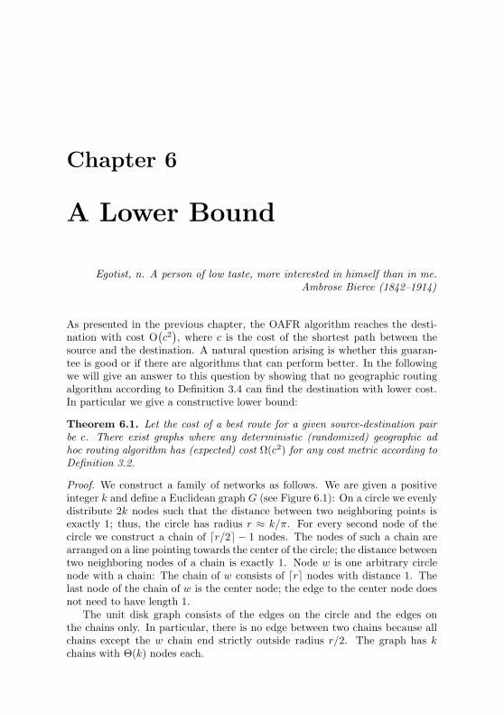
Theorem 6.1. Let the cost of a best route for a given source-destination pairbe c. There exist graphs where any deterministic (randomized) geographic adhoc routing algorithm has (expected) cost Ω(c2) for any cost metric according toDefinition 3.2.

Proof. We construct a family of networks as follows. We are given a positiveinteger k and define a Euclidean graph G (see Figure 6.1): On a circle we evenlydistribute 2k nodes such that the distance between two neighboring points isexactly 1; thus, the circle has radius r ≈ k/π. For every second node of thecircle we construct a chain of dr/2e − 1 nodes. The nodes of such a chain arearranged on a line pointing towards the center of the circle; the distance betweentwo neighboring nodes of a chain is exactly 1. Node w is one arbitrary circlenode with a chain: The chain of w consists of dre nodes with distance 1. Thelast node of the chain of w is the center node; the edge to the center node doesnot need to have length 1.

The unit disk graph consists of the edges on the circle and the edges onthe chains only. In particular, there is no edge between two chains because allchains except the w chain end strictly outside radius r/2. The graph has kchains with Θ(k) nodes each.

42 CHAPTER 6. A LOWER BOUND

w

Figure 6.1: Lower bound graph.

We route from an arbitrary node on the circle (the source s) to the centerof the circle (the destination t). An optimal route between s and t follows theshortest path on the circle until it hits node w, and then directly follows w’schain to t with link cost c ≤ k +r+1 ∈ O(k). A routing algorithm with routingtables at each node will find this best route.

A geographic routing algorithm, in contrast, needs to find the “correct”chain w. Since there is no routing information stored at the nodes, this canonly be done by exploring the chains. Any deterministic algorithm needs toexplore the chains in a deterministic order until it finds the chain w. Thus, anadversary can always place w such that w’s chain will be explored as the lastone. The algorithm will therefore explore Θ(k2) (instead of only O(k)) nodes.

The argument is similar for randomized algorithms. By placing w accord-ingly (randomly!), an adversary forces the randomized algorithm to exploreΩ(k) chains before chain w with constant probability. Then the expected linkcost of the algorithm is Ω(k2).

As all edges (but one) in our construction have length 1, the cost values inthe Euclidean distance, the link distance, and the energy metrics are equal. Asfor any fixed cost metric c′(·) according to Definition 3.2 c′(1) is also a constant,the Ω(c2) lower bound holds for all according metrics.

Note that our lower bound holds generally, not only for Ω(1)-graphs. As wewill show in Chapter 9, however, a similar lower bound proves that in generalgraphs the cost metrics according to Definition 3.2 fall into two classes.

43

Given this lower bound, we can now state that OAFR is asymptoticallyoptimal for unit disk graphs in the Ω(1)-model.

Theorem 6.2. Let c be the cost of an optimal path for a given source-destinationpair on a unit disk graph in the Ω(1)-model. In the worst case, the cost for ap-plying OAFR to find a route from the source to the destination is Θ(c2). Thisis asymptotically optimal.

Proof. This theorem is an immediate consequence of Theorems 5.3 and 6.1.

44 CHAPTER 6. A LOWER BOUND

Chapter 7

Combining Greedy and

Face Routing

Skiing combines outdoor fun with knocking down trees with your face.Dave Barry (*1947)

A greedy routing approach as presented in Chapter 4 is not only worth beingconsidered due to its simplicity in both concept and implementation. Above allin dense networks such an algorithm can also be expected to find paths of goodquality efficiently; here, the straightforwardness of a greedy strategy contrastshighly the inflexible exploration of faces inherent to face routing. For practicalpurposes it is inevitable to improve the performance of a face routing variant,for instance by leveraging the potential of a greedy approach.1

In this chapter we will present two algorithms combining greedy and facerouting. The GOAFR algorithm introduces the principal concept employed tointegrate these two approaches. Later, the GOAFR+ algorithm is not onlyproved to be worst-case optimal but—due to its additional improvements—willbe shown in Chapter 8 to outperform all previously proposed geographic routingalgorithms in average-case networks.

7.1 GOAFR: Greedy OAFR

A possible combination of greedy routing and our OAFR algorithm forms GreedyOther Adaptive Face Routing GOAFR (pronounced as “gopher”). In principle

1Interestingly, simple non-geographic flooding of the network with exponentially increas-ing time-to-live values achieves the same worst-case efficiency as the face routing algorithmsdescribed in the previous chapter if we allow the network nodes to temporarily store floodingstate information in some additional bits. Only additional average-case assessment as car-ried out later in Chapter 8 will display the main advantages of routing algorithms combininggreedy and face routing over such simplistic approaches.

46 CHAPTER 7. COMBINING GREEDY AND FACE ROUTING

v1

v2s tF

Figure 7.1: Starting at s, GOAFR proceeds in greedy mode until reaching thelocal minimum v1. The algorithm switches to face routing mode and exploresthe boundary of face F to find v2, the node closest to t on F ’s boundary.GOAFR falls back to greedy mode and finally reaches t. Note that GOAFR’sellipse has been omitted for simplicity.

greedy routing is used as long as possible. Local minima potentially met un-derway are escaped from by use of OAFR (Figure 7.1). After specifying thealgorithm, we will show that GOAFR retains OAFR’s asymptotic optimality.

The greedy steps taken in the following specification of the GOAFR algo-rithm correspond to the steps described as the Greedy Routing algorithm inChapter 4.

Greedy Other Adaptive Face Routing GOAFR

0. Initialize E to be the ellipse with foci s and t the length of whose majoraxis is 2 · |st|; start at s.

1. Perform greedy steps until either reaching t or a local minimum um. If thenext step leads beyond E , double the length of E ’s major axis. If reachinga local minimum, proceed with step 2 starting at um.

2. Execute OAFR on the first face F only. Double the length of E ’s majoraxis as long as necessary.

3. Terminate if OAFR reaches t. If OAFR detects disconnection, report soto s (by use of GOAFR). Otherwise (OAFR has found—after completeexploration of F ’s boundary within E in its current size—a node v with|vt| < |umt|) continue with step 1 at the node closest to t found by OAFR.

In order to show that the cost expended by GOAFR is bounded, we firstprove that the maximal size of the ellipse E is related to the length of a shortestpath between s and t.

7.1. GOAFR: GREEDY OAFR 47

Lemma 7.1. If s and t are connected, the major axis of E in GOAFR will notexceed 2 ·max(cd(p

∗) , 3|st|), where cd(p∗) is the Euclidean length of an optimal

path (with respect to the Euclidean metric).

Proof. According to the definition of an ellipse as the locus of all points havingthe same sum of distances from the two foci, the ellipse E with major axis lengthc contains all paths of Euclidean length at most c. With the doubling strategyin OAFR, the biggest ellipse employed in this “subalgorithm” of GOAFR willhave a major axis not longer than 2 · cd(p

∗). Additionally the Greedy Routingpart of GOAFR might walk (almost) along the boundary (but is always on theinside) of D(t, |st|), the disk centered at t and with radius |st|. E with major axislength 3|st| is the smallest ellipse with s and t as foci which completely containsD(t, |st|). Combining the OAFR part, the GR part, and the fact that the ellipsemight get twice as big as the smallest possible ellipse, the lemma follows. Notethat these considerations hold with slight modifications for any (sufficientlysmall) start value and increment factor for the major axis length of the ellipse.If these two parameters are chosen as in the definition of GOAFR, the boundon the length of the major axis can be improved to max(2|p∗|, 4|st|).

In the following lemma we consider the execution of GOAFR within anellipse of fixed size.

Lemma 7.2. For an ellipse E with fixed major axis length c, GOAFR traversesat most O

(c2)

edges.

Proof. GOAFR consists of face routing steps (more specifically OBFR) andof greedy routing steps. Each of these steps (a greedy step or the completeexploration of a face) brings us to a node closer to the destination t. Thenumber of greedy steps is bounded by O

(c2)

(cf. Lemma 4.1). As in OBFR,each face is explored at most once and hence each (Gabriel Graph) edge is usedat most four times in a face routing step. Combined, this proves the lemma.

This leads to the conclusion that the cost of GOAFR is bounded by thesquared cost of the optimal path:

Theorem 7.3. If s and t are connected, GOAFR reaches t with cost O(c2(p∗)

).

This is asymptotically optimal. If s and t are not connected, GOAFR reportsso.

Proof. If s and t are connected, the lemma is a consequence of Lemma 7.1(using that |st| ≤ cd(p

∗) and Lemma 7.2 combined with the fact that the ellipseaxis lengths form a geometric sequence (cf. proof of Theorem 5.3) and theasymptotic equivalence of all cost metrics according to Definition 3.2. Thelower bound discussed in Chapter 6 proves the asymptotic optimality. If s andt are not connected, the node detecting this (after a face routing step whichdoes not yield a node closer to t) sends the result back to s by means of thesame algorithm.


Remark Similar to OAFR, GOAFR detects disconnectivity of s and t withcost at most O(n′ log n′), where n′ is the number of nodes in the network com-ponent containing s.

7.2 GOAFR+: Improving GOAFR

Having shown the concept of combining greedy and face routing, we will presentin this section the GOAFR+ algorithm (pronounced as “gopher-plus”), whichforms a refinement of the GOAFR algorithm. The primary reason for the modi-fications resulting in GOAFR+ is their leading to better performance in average-case networks, which will be shown in Chapter 8. At the same time, however,the asymptotic optimality of the GOAFR algorithm is preserved, as proved afterthe following specification of GOAFR+.

7.2.1 The GOAFR+ Algorithm

Similar to GOAFR, the GOAFR+ algorithm is a combination of greedy routingand face routing. Whenever possible, the algorithm tries to route in a greedymanner; in order to overcome local minima with respect to the distance fromthe destination, face routing is employed.

In face routing mode, GOAFR+ restricts the searchable area in a similarway as GOAFR. Our simulations (as discussed later in Chapter 8) showed thatchoosing a circle centered at the destination t instead of an ellipse and aboveall gradually reducing its radius while the message approaches t improves theaverage-case performance.

More importantly, for average-case considerations, the algorithm should fallback to greedy routing as soon as possible after escaping the local minimum.This is suggested by the observation that greedy forwarding is—especially indense networks—more efficient than face routing in the average case. If GOAFRtraverses the complete boundary of a face—once it is in face routing mode—, GOAFR+ tries to avoid doing so and to return to greedy routing as earlyas possible. As will be illustrated in Chapter 8, this must not be done toosimplistically—such as whenever the algorithm in face routing mode is closer tothe destination than the escaped from local minimum—, as this would happenat the expense of the algorithm’s asymptotic optimality. In order to preservethis property, the GOAFR+ algorithm employs two counters p and q to keeptrack of how many of the nodes visited during the current face routing phaseare located closer to the destination (counted with p) and how many are atleast as far from the destination (counted with q) than the starting point ofthe current face routing phase; as soon as a certain fallback condition holds,GOAFR+ continues in greedy mode.

Figure 7.2 provides an illustration to the following specification of the GOAFR+

algorithm.

7.2. GOAFR+

: IMPROVING GOAFR 49

s u

C

v

w t

F

Figure 7.2: The GOAFR+ algorithm starts from s in greedy mode. At node u,it reaches a local minimum, a node without any neighbors closer to t. GOAFR+

switches to face routing mode and begins to explore the boundary of face F (inclockwise direction). At node v the algorithm hits the bounding circle C andturns back to continue the exploration of F ’s boundary in the opposite direction.After each step the counters p and q are updated. At node w the fallbackcondition p > σ q holds (p = 2, q = 4 with the assumption 1/4 ≤ σ < 1/2);GOAFR+ falls back to greedy mode and continues to finally reach t. (Gradualreduction of C’s size during GOAFR+’s execution is not shown.)

GOAFR+ The algorithm parameters ρ0, ρ, and σ are chosen prior to thestart of the algorithm and remain constant throughout the execution. For thealgorithm to work correctly, these parameters have to comply with the condi-tions 1 ≤ ρ0 < ρ and 0 < σ.2

0. Begin at s. Initialize C to be the circle centered at t with radius rC :=ρ0 |st|.

1. (Greedy Routing Mode) Repeat taking greedy steps until either reach-ing t or a local minimum. In the former case the algorithm terminates, inthe latter case continue with step 2. Whenever possible, reduce C’s radius(rC := rC/ρ) as long as the currently visited node stays within C.

2. (Face Routing Mode) Let ui be the currently visited local minimum.Start exploring the boundary of Fi, the face containing the connecting lineuit in the immediate environment of ui. When completing Fi’s explorationand returning to ui, advance to the node visited so far closest to t andcontinue with step 1. If—after F ’s complete exploration—no visited node

2In our simulations ρ0 = 1.4, ρ =√

2, and σ = 1

100proved to be good choices for practical

purposes.


is closer to t than ui, report graph disconnection to s (using GOAFR+).During the exploration of Fi’s boundary use two counters p and q to keeptrack of the number of nodes visited on Fi’s boundary: p counts the nodescloser to t than ui and q the nodes not located closer to t than ui. Takea special action if one of the following conditions holds:

2a. Hitting C for the first time, turn back and continue exploring Fi’sboundary in the opposite direction.

2b. C is hit for the second time: If none of the visited nodes is closerto t than ui, enlarge C (rC := ρ rC) and continue with step 2 as ifhaving started from ui. Otherwise advance to the node visited so farclosest to t and continue with step 1.

2c. If p > σ q, that is, we have visited (up to a constant factor σ) morenodes on Fi’s boundary closer to t than nodes not closer to t, advanceto the node seen so far closest to t (if this is not the currently visitednode) and continue with step 1.

With this description of the GOAFR+ algorithm, we can now proceed toshowing that its worst-case performance is asymptotically equivalent to the oneof GOAFR.

7.2.2 GOAFR+ is Asymptotically Optimal

GOAFR+ uses a circle C centered at t to restrict itself to a searchable area.During the algorithm execution the radius rC is adapted in predefined stepsaccording to the current distance from t. In particular, the values potentiallyassumed by rC form a geometric sequence rCi

= rmax ( 1ρ )i, i = 0, ..., k, where

rmax depends on the length and the shape of the optimal path from s to t (cf.proof of Theorem 7.7) and ρ is one of GOAFR+’s predefined constant algorithmparameters. Since rC can both increase and decrease during algorithm execu-tion, the steps taken in a circle Ci with radius rCi

need not occur consecutively.In the following we consider the steps taken by the algorithm in a fixed circleCi.

Lemma 7.4. If s and t are connected within the circle Ci, GOAFR+ reachest. If s and t are not connected within Ci, GOAFR+ detects so.

Proof. We first assume there is a connection from s to t within Ci. For thedefinition of a round we distinguish three cases: According to the current al-gorithm execution, a round can be either a) a greedy step, b) a face routingphase terminated by early fallback, or c) a face routing phase terminated afterexploration of the complete boundary of the current face and advancing to thenode closest to t. We show that after every round the algorithm is closer tot than before that round: This holds in case a) since a greedy step can onlyreduce the distance to t, and in case b), as the fallback condition can only holdimmediately after incrementing the counter p (that is after visiting at least one

7.2. GOAFR+


node closer to t) and since the algorithm then advances to the node seen so farclosest to t; in case c), the algorithm approaches t since the boundary of thecurrently explored face—this face contains in its interior points closer to t thanwhere this round started—contains a point closer to t if and only if there isa connection to t. (Note that again the remark made after Lemma 5.1 holds:Graphs can be constructed where a face F ’s boundary contains points but notnodes that are closer to t than a given boundary node, in which case the algo-rithm could fail. Since we employ the Gabriel Graph, such cases can howevernot occur: The algorithm can forward to a face boundary’s node closest to t.)As the algorithm reduces the distance to the destination in each round, it finallyreaches t.

If s and t are not connected within Ci, GOAFR+—in face routing mode—either hits Ci twice without finding a node closer to t (in which case the algo-rithm will continue on a bigger circle, which is beyond the scope of this lemma),or it explores the complete boundary of the current face (cf. above case c))without finding a node closer to t, which is the case if and only if s and t arenot connected at all.

Having shown that GOAFR+ reaches the destination, we can now prove inseveral steps that its cost is bounded. We first consider the cost expended whentraversing the boundary of a given face within a circle of fixed size.

Lemma 7.5. Let c′F (GOAFR+) be the cost of all face routing steps taken whenexploring the boundary of face F within the circle Ci. c′F (GOAFR+) is lessthan γ cF for a constant γ and with cF being the total cost of traversing F ’sboundary once.

Proof. We first show that the lemma holds for the link distance metric, c(e) ≡ 1for any edge e: The total number of edges traversed by GOAFR+ when exploringF is less than γc`F

, where c`Fis the number of edges traversed when traveling

around F once.

We assume that the boundary of face F is involved in k face routing rounds,and that for 1 ≤ j ≤ k, sj is the node where round j is started. Let pj and qj

be the final values of the counters p and q, respectively, in round j. Accordingto the fallback condition in step 2c of the algorithm we have pj > σ qj . Let Pj

and Qj be the sets of nodes visited in round j closer to t than sj and at leastas far from t as sj , respectively. Since a node can be counted for a second timeafter hitting Ci, we have |Pj | ≤ pj ≤ 2 |Pj | and |Qj | ≤ qj ≤ 2 |Qj |. Furthermorewe define Nj to be the set of nodes newly visited in round j. Since after eachround—a greedy step or the exploration of a face—the algorithm is strictlycloser to t than before that round, all nodes closer to t must be newly visitedones, that is Pj ⊆ Nj . Since we also have to account for the steps taken by thealgorithm possibly proceeding—once the fallback criterion holds—to the nodeseen so far closest to t, the number of steps taken in round j is not greater than


2 (pj + qj). In summary we obtain for the total cost of the algorithm exploringF ’s boundary:

k∑

j=1

2 (pj + qj) <

k∑

j=1

2 (1 +1

σ) pj ≤

k∑

j=1

4 (1 +1

σ) |Pj |

≤k∑

j=1

4 (1 +1

σ) |Nj | ≤ 4 (1 +

1

σ) c`F

,

the last step following from∑k

j=1 |Nj | ≤ c`F.

If the fallback criterion never holds during F ’s exploration (which is onlypossible in the final round for F ), the algorithm traverses F ’s complete boundaryand advances to the node closest to t, which incurs additional cost less than2 c`F

.The lemma holds for the link distance metric. Since the algorithm is assumed

to run in the Ω(1)-model, the lemma also holds for any other cost metric (cf.Chapter 3).

With this lemma, the overall cost—in greedy and in face routing mode—expended in a given circle of fixed size can be bounded:

Lemma 7.6. The total cost of the steps taken by GOAFR+ within the circleCi with radius rCi

is in O(r2Ci

).

Proof. According to the previous lemma we have c′F (GOAFR+) ≤ γ cF for allsteps performed in face routing mode. Summing up over all faces in Ci, weobtain ∑

F∈Ci

c′F (GOAFR+) < γ ·∑

F∈Ci

cF ≤ γ · 2∑

e∈Ci

c(e),

the last step following from the fact that each edge e is adjacent to at mosttwo faces. To account for the greedy steps, we add another

∑e∈Ci

c(e) in orderto obtain the total cost expended in Ci since any edge can be traversed atmost once in greedy mode (each round—a greedy step or the exploration ofa face—taking the algorithm strictly closer to t). Since we employ a planargraph, with the fact that (in a graph with more than three edges) each faceis adjacent to at least three edges and using the Euler polyhedral formula,we obtain that |Ei| ∈ O(|Vi|), where |Ei| is the number of edges and |Vi| thenumber of nodes in Ci (cf. proof of Lemma 5.1). The lemma finally followswith

∑e∈Ci

c(e) ∈ O(|Ei|)—resulting from the equivalence of the link distancemetric with any other metric in the Ω(1)-model (cf. Chapter 3)—and the factthat in the Ω(1)-model the number of nodes in a given region is proportional toits size (cf. proof of Lemma 5.2).

As described above, GOAFR+ employs a set of bounding circles whose radiiform a geometric sequence. This together with the fact that the maximumradius is bounded by the Euclidean length of an optimal path from s to t, leadsto the following theorem.

7.2. GOAFR+


Theorem 7.7. Let p∗ be an optimal path from s to t. In the Ω(1)-model,GOAFR+ reaches t with cost O

(c2(p∗)

)if s and t are connected, which is

asymptotically optimal. If s and t are not connected, GOAFR+ reports so tothe source.

Proof. Let cd(p∗) be the Euclidean length of a shortest path from s to t. If s

and t are connected, the circle centered at t and with radius cd(p∗) completely

contains p∗. Since GOAFR+ only enlarges the bounding circle if it does notcontain a path from s to t, and according to GOAFR+’s radius update policywith the constant factor ρ, the maximum radius reached is smaller than ρ cd(p

∗).In order to compute the total cost of the algorithm, we add up the cost expendedin each used circle. According to Lemma 7.6 it is sufficient to consider the sumof the squared radii of all employed circles. Let rmax be the radius of the largestused circle. For some k ≥ 0 the areas of all used circles sum up to

k∑

i=0

[rmax ·

(1

ρ

)i]2

=1 −

(1ρ

)2(k+1)

1 −(

1ρ

)2 r2max

<1 −

(1ρ

)2(k+1)

1 −(

1ρ

)2 (ρ cd(p∗))2

∈ O(cd(p

∗)2).

With the equivalence of cost metrics—including the Euclidean metric—in theΩ(1)-model, this holds for any metric. Asymptotic optimality follows from thelower bound example in Chapter 6.

If s and t are not connected, GOAFR+ detects so (case c) in proof ofLemma 7.4) and reports back to the source using the same algorithm.

Remark Like OAFR and GOAFR, GOAFR+ detects and reports disconnec-tivity of s and t with cost at most O(n′ log n′), where n′ is the number of nodesin the network component containing s.

Having presented different geographic routing algorithms and proved theirasymptotic worst-case properties, we will discuss and compare the performanceof these algorithms and of other heuristic combinations of greedy and face rout-ing in average-case networks in the following chapter.


Chapter 8

Greedy and Face Routing

in Average-Case Networks

It is even harder for the average apeto believe that he has descended from man.

Henry Louis Mencken (1880–1956)

In the previous three chapters we showed that it is not only possible to define aworst-case-optimal geographic routing algorithm exploiting the concept of facerouting, but also to combine the notions of greedy routing and face routingin algorithms which conserve worst-case optimality. The approach to combinegreedy and face routing was thereby driven by the observation that—whenmoving our focus away from worst-case networks to average-case scenarios—greedy routing lends itself as an efficient routing concept. In this chapter weanalyze the validity of the hypothesis that a combination with greedy routingcan improve performance in average-case networks.

In particular we describe performance measurements taken in simulationsnot only of the algorithms described in the previous chapters but of a varietyof face routing algorithms and their combinations with the greedy approach.We also present a number of graph characteristics yielding deeper insight in thebehavior of the routing algorithms. Before focusing on our routing algorithms,we will present a basic observation.

8.1 The Role of Network Density

In this section we will discuss the correspondence between network density andsubstantial network properties in the context of routing. In particular we pointout the importance of the chosen density range for the simulation of routingalgorithms.

56 CHAPTER 8. AVERAGE-CASE NETWORKS

1

1.1

1.2

1.3

1.4

1.5

1.6

1.7

1.8

1.9

0 5 10 15

Network Density [nodes per unit disk]

Sh

ort

est

Pat

h S

pan

0

0.1

0.2

0.3

0.4

0.5

0.6

0.7

0.8

0.9

1

Fre

qu

ency

Figure 8.1: Connectivity rate (dashed), greedy success rate (dotted, both plot-ted against the right y-axis), and mean shortest path span (solid, plotted againstthe left y-axis).

Our measurements were carried out on the unit disk graph of networks withnodes randomly and uniformly placed on a square with 20 units side length.For each density value (denoted in nodes per unit disk on the x-axis of Fig-ure 8.1), we generated 2000 such random networks and chose the source s andthe destination t randomly.

In particular we measured three parameters for each density:

- Connectivity rate: In how many cases are s and t connected?

- Greedy success rate: How often does the greedy algorithm GR alone reacht?

- Shortest path span: The ratio between cd(p∗), the Euclidean length of

the shortest (Euclidean) path, and |st|, the Euclidean distance betweens and t. Note that the shortest path span is only defined if s and t areconnected.

Figure 8.1 depicts our measured values of these three parameters over adensity range of 0.3 to 20 nodes per unit disk. The connectivity and greedysuccess rate values are plotted against the right; the mean of the measuredshortest path span values is plotted against the left y-axis.

8.1. THE ROLE OF NETWORK DENSITY 57

The network connectivity curve (dashed line) shows that the density spansfrom one extreme to the other. At very low network densities, nodes are sosparsely placed that we observe almost no connectivity at all. On the other endof the scale, s and t are virtually always connected. The transition betweenthese two extremes takes place in a relatively narrow density range betweenapproximately 3 and 7 nodes per unit disk. Network connectivity—above all inthis transition range—is one of the main issues in percolation theory [29, 73]. Inthe following we will justify why this is a mandatory range for routing algorithmsimulations to take place.

Of high importance for our greedy/face routing combinations is the greedysuccess rate (dotted line). Since network connectivity is a requirement for anyrouting algorithm, the greedy success rate lies strictly below the connectivityrate curve. For high network densities on the other hand, a gap big enough toform a local minimum for greedy routing will only be generated with low prob-ability; greedy routing can be expected to almost always reach the destination.

The third curve in Figure 8.1 (solid line) represents the mean shortest pathspan, that is, for each density the curve value is the mean of the ratio valuesbetween the Euclidean length of the shortest path and the Euclidean distancebetween s and t over all generated networks. For very low densities this valueis close to 1 due to low network connectivity: The shortest path span is onlydefined if s and t are connected, which is rarely ever the case here. If howevers and t are connected, they are with high probability close together or evenneighbors, in which case the shortest path span is equal to 1. The low valuesfor high densities, on the other hand, can be explained by the fact that withincreasing density the shortest path will more and more closely follow the directconnecting line st due to the rising number of nodes in st’s vicinity.

Between these two extremes the shortest path span forms an almost bell-shaped curve in the network density range approximately between 3 and 6 nodesper unit disk. Informally put, this is the only density region where the shortestpath is usually much longer than the direct connection between s and t (cf.Figure 8.2). This specific quality identifies this region as “critical” for routingalgorithms. Here, finding a good path at low cost becomes a nontrivial taskand a real challenge for geographic routing. It also appears that for the crit-ical density region the effect of introducing “artificiality” by placing networknodes uniformly remains acceptably low: The density is relatively heteroge-neous, which reflects the situation to be expected in reality more closely thana homogeneous placement of nodes that would occur for higher network densi-ties. Furthermore, it is not astonishing that simulations carried out on densenetworks (such as for the GPSR geographic routing algorithm with approxi-mately 21.8 nodes per unit disk in [57]) display very good results with respectto both the quality of the discovered path and algorithm performance.

In the following we will therefore mainly focus on this critical density rangearound 4.5 nodes per unit disk in our algorithm simulations.


Figure 8.2: Example of generated (Gabriel) graph at critical network density4.71 (≈ 1.5 π) nodes per unit disk (600 nodes on 20 by 20 units field). Most of thenodes are connected; for most pairs of nodes, however, the shortest connectingpath is significantly longer than their Euclidean distance.

8.2 Algorithm Overview

Before presenting our simulation results we will introduce all simulated algo-rithms for the sake of clarity. Figure 8.3 contains an “algorithm family tree”,a graphical representation of the conceptual relations between the single algo-rithms.

The basis of this algorithm family is formed by two fundamental algorithms:

- FR is the traditional Face Routing algorithm as introduced in [61] andoutlined in Section 5.1. On a planar graph one face after the other iscompletely explored in order to find intersections of its boundary withst, the line connecting s and t. Along this line the algorithm graduallyproceeds and finally reaches t.

- GR proceeds in each step to the neighbor closest to the destination, asdescribed in Chapter 4. Note that this algorithm—as opposed to all othersimulated algorithms—cannot guarantee to reach t.

8.2. ALGORITHM OVERVIEW 59

AFR

GAFR

GAFRFI

GOAFR− GAFR−

OAFR

GOAFR

GOAFRFC

GOAFR+

FR(Face Routing)

(Greedy Routing)GR

GFR

OFR

FC=GFR

AFRFI

GFG/GPSR

Figure 8.3: Algorithm relation overview. The basis for all simulated routingalgorithms is formed by FR and GR. Algorithms in elliptic shapes use a bound-ing ellipse (GOAFR+ using a bounding circle). A double ellipse representsasymptotic optimality. Algorithms in dashed circles have been introduced forthe concept only, without simulations.

In Section 5.3 we introduced OFR, a variant of FR in the sense that it doesnot switch to a new face along the line st, but at the point closest to t on theboundary of the currently explored face. OFR builds the basis for a completeline of algorithms; it has however not been implemented for our simulations.Extending the FR and OFR algorithms by adaptive bounding ellipses, we obtainAFR and OAFR:

- In AFR (cf. Section 5.2), Face Routing is extended by the concept of abounding ellipse whose size is iteratively incremented as required. Notethat—as an improvement over the original description—our implementa-tion of the AFR algorithm does not return to the source before increment-ing the ellipse size.

- In OAFR, as described in Section 5.3, face routing is not performed alongthe st line. Instead, the algorithm explores a face for the node on itsboundary with the least distance from t, where it proceeds to the nextface.

Introduced as a building block for later use, the algorithm AFRFI uses a heuris-tic to try to switch to the next face earlier than AFR:


- AFRFI (AFR + “First Intersection” heuristic)—in contrast to AFR—does not necessarily explore complete faces but already switches to thenext face when first meeting an intersection with st closer to t than wherethe current face’s exploration started.

The remaining algorithms all include greedy routing phases. GOAFR com-bines GR with OAFR; GAFR employs GR and AFR. The GFR algorithm isintroduced for the concept only, that is without simulations.

- The GOAFR algorithm is described in detail in Section 7.1. It employs GRas long as possible and overcomes potential local minima by explorationof one face with OAFR.

- GAFR combines greedy routing and AFR. Local minima are circumventedusing the AFR algorithm for one face before returning to greedy mode.In analogy to GOAFR, GAFR retains the same ellipse throughout itsexecution, apart from enlarging it when necessary.

The algorithms GOAFR– and GAFR– are minor variations of GOAFR andGAFR, respectively.

- GOAFR–’s only difference compared to GOAFR consists in its use ofa bounding ellipse exclusively when in face routing mode. Each timestarting a face routing phase at node u, the ellipse is initialized around uand t.

- GAFR– reinitializes its bounding ellipse for each face routing phase aroundthe new starting point and t; otherwise it is identical to GAFR.

Similarly as in AFRFI , the algorithms GAFRFI , GOAFRFC , and GFG/GPSRemploy heuristics to terminate the exploration of the current face and conse-quently fall back to greedy mode earlier than GAFR, GOAFR, or GFR, respec-tively.

- GAFRFI ’s only difference compared to GAFR is its use of AFRFI insteadof AFR: The next greedy phase is started already when meeting the firstintersection with st.

- GOAFRFC (GOAFR + “First Closer” heuristic) uses GR and OAFR, butfalls back to greedy mode even earlier, that is at the first node closer to tthan where the face routing phase started.

- GFG/GPSR was introduced in [14] and [57]. Apart from the fact that itdoes not bound its searchable area, it is identical to GOAFRFC.

Finally, the GOAFR+ algorithm also tries to return from face routing to greedyrouting as early as possible, goes however beyond GOAFRFC in that it employsa counter mechanism.

8.2. ALGORITHM OVERVIEW 61

Character Stands for Comment

R Routing occurs in all algorithm namesF Face algorithms employing face routingG Greedy algorithms employing greedy routingA Adaptive algorithms using a bounding ellipseO Other algorithms using OFR– starts face routing phases with small ellipse

. . . RFI First Intersection uses “First Intersection” heuristic. . . RFC First Closer uses “First Closer” heuristic

+early fallback with counters; uses circlewith gradually reduced radius (only usedin GOAFR+)

Table 8.1: Algorithm naming system.

- GOAFR+ as described in detail in Section 7.2 applies a node countermechanism in order to decide when to fall back to greedy routing and thuspreserves GOAFR’s asymptotic worst-case optimality. Furthermore—incontrast to the other algorithms using an ellipse—it restricts its searchablearea with a circle centered at t whose size is gradually reduced whileapproaching the destination.

In order to distinguish the single algorithms, we introduced a naming sys-tem in which each character contained in an algorithm name represents aconcept (Table 8.1). Note that the abbreviation GFG/GPSR (Greedy-Face-Greedy/Greedy Perimeter Stateless Routing) [14, 57] does not correspond withour naming system. In our system GFG/GPSR would be named GFRFC.

Table 8.2 summarizes all simulated algorithms and compares them withrespect to five characteristics:

- Type: The algorithms fall into three main classes: Pure face routing al-gorithms (fr), the GR algorithm (gr), and combinations thereof (gr +fr).

- With Bounding Ellipse: Apart from FR and GFG/GPSR all algorithmsbound their searchable area (by an ellipse or, in the case of GOAFR+, bya circle).

- With Heuristic: In face routing mode (G)AFRFI, GOAFRFC, and GFG/-GPSR apply heuristics in order to proceed with greedy routing withoutexploring the complete boundary of a face. Doing so, however, thesealgorithms lose their asymptotic optimality.

- Retains Ellipse: This property is only applicable to gr + fr algorithmswith a bounding ellipse. Most of these algorithms only use a bounding


ellipse during their greedy routing phase. GOAFR and GAFR in con-trast retain—apart from incrementing its size—the same ellipse through-out their complete execution.

- Asymptotically Optimal: As outlined in Section 5.2, AFR has previouslybeen proved to be asymptotically optimal. In the subsequent two sectionswe showed that also OAFR and GOAFR are asymptotically optimal geo-graphic routing algorithms. Note the correspondence between algorithmsusing heuristics and asymptotic optimality. Only by means of a nodecounter scheme can the GOAFR+ algorithm preserve worst-case optimal-ity while attempting to fall back to greedy routing without traversing thecomplete boundary of the currently visited face.

Note that GR is the only algorithm that may fail to reach t. All other simulatedalgorithms are guaranteed to find the destination.

8.3 Routing Algorithm Simulations

We are now ready to present the results of our routing algorithm simulations.As in the measurements presented in Section 8.1, we generated networks onsquare fields of side length 20 units by distributing network nodes randomly anduniformly. For every simulation series, the number of nodes was determinedaccording to the chosen network density. For each considered network, thesource s and the destination t were also chosen randomly.

In order to judge the practicability of an algorithm we introduced the nor-malized cost costA(N, s, t) of an algorithm A in a network N given a source sand a destination t as

costA(N, s, t) :=sA(N, s, t)

c`(p∗` (N, s, t)),

where sA(N, s, t) is the number of steps taken by algorithm A in network Nfinding a route from s to t (which is in our case, with all simulated algorithms,equal to the number of sent messages); c`(p

∗` (N, s, t)) is the (hop) length of the

shortest path (with respect to the hop metric) between the source s and thedestination t in N .

Counting the steps taken by an algorithm A corresponds to the link (orhop) metric of A’s path. There are two reasons for choosing the link metric forour simulations. First, the link metric is a model for currently employed radionetwork technology: In most communication standards (such as IEEE 802.11),radio devices transmit with a fixed—at least not dynamically adapted—powerlevel. Second—assuming that sending a message to a neighboring node takesa certain period of time independent of its distance—the link length of a pathforms a good measure for the latency of a message traveling along that path.

Our objective was to measure the performance of the routing algorithmswithout any interference of possible side effects of other communication layers.

8.3

.R

OU

TIN

GA

LG

OR

ITH

MSIM

ULAT

ION

S63

Algorithm Name Type

WithBound-

ingEllipse

WithHeuristic

RetainsEllipse

Asympto-tically

Optimal

Comment

FR fr no no - no Face Routing as described in Section 5.1

AFR fr yes no - yes Adaptive Face Routing (Section 5.2)

AFRFI fr yes yes - noAFR, but switches to next face at first intersection withst

OAFR fr yes no - yes Other Adaptive Face Routing (Section 5.3)

GOAFR gr + fr yes no yes yes Greedy Other Adaptive Face Routing (Section 7.1)

GOAFR– gr + fr yes no no noGOAFR, but starts face routing phases with small el-lipse

GAFR gr + fr yes no yes no Greedy + AFR

GAFR– gr + fr yes no no noGreedy + AFR, but starts face routing phases withsmall ellipse

GAFRFI gr + fr yes yes no noGAFR, but falls back to greedy routing when first in-tersecting st

GOAFRFC gr + fr yes yes no noGOAFR, but falls back to greedy routing when meetingfirst node closer to t than where AFR phase started

GFG/GPSR gr + fr no yes - noGreedy-Face-Greedy/Greedy Perimeter StatelessRouting [14, 57]: GOAFRFC without bounding ellipse

GOAFR+ gr + fr yes -* -* yesGOAFR+ algorithm as defined in Section 7.2. *Usescounters for early fallback and concentric circles

GR gr no - - - out of competition, since reaching of t not guaranteed

Table 8.2: Classification of simulated routing algorithms. The GOAFR algorithm, for instance, is a greedy/face routingcombination, employs a bounding ellipse, does not use a heuristic for early fallback to greedy mode, keeps the ellipse whenswitching from one mode to the other (does not restart with a small ellipse), and is asymptotically optimal. The GR algorithmis listed for completeness, but runs out of competition, since it does not guarantee to reach the destination.


0

2

4

6

8

10

12

14

16

18

20

0 5 10 15


Mea

n A

lgo

rith

m C

ost

0

0.1

0.2

0.3

0.4

0.5

0.6

0.7

0.8

0.9

1

Fre

qu

ency

Figure 8.4: Algorithm performance overview. Mean cost values of FR (upperdashed line), AFR (upper solid), OAFR (lower dashed), and AFRFI (lowersolid). All greedy/face routing combinations (including GOAFR, GOAFR+,and GFG/GPSR) are shown in dotted lines (for details see Figure 8.5). Thenetwork connectivity and greedy success rates (gray) are plotted against theright y-axis for reference (cf. Section 8.1).

We therefore assumed an ideal environment with collisionless MAC layer andpostulated all position information required by the geographic routing model—a node’s own and its direct neighbors’ positions as well as information aboutthe destination position being present at the source—to be available withoutadditional communication overhead. We furthermore assumed the routing al-gorithms to execute fast compared to possibly moving network nodes; nodemovement was consequently not simulated. The measurements were carriedout on a custom simulation environment.

Figure 8.4 shows for each simulated algorithm A its mean cost value, definedas

costA :=1

k

k∑

i=1

costA(Ni, si, ti)

over all k = 2000 generated triples (Ni, si, ti) for network densities ranging from0.3 to 20 nodes per unit disk. For reference to the density range, the networkconnectivity and greedy success rates are plotted against the right y-axis.

8.3. ROUTING ALGORITHM SIMULATIONS 65

For very low network densities all algorithms perform more or less equallywell, for the same reason that keeps the shortest path span low (see Section 8.1):The source s and the destination t are rarely ever connected; if however theyhappen to be connected, they are very likely direct neighbors.

On the other end of the density scale, two classes of algorithms can bedistinguished.

- The cost values of all algorithms solely employing a variant of face rout-ing approach a linearly growing curve. The general growth of the costof these algorithms towards infinity can be explained by the fact that wemeasure the hop metric cost values of the algorithm paths together withtwo reasons: FR, AFR, and OAFR route along complete faces; the ex-pected number of such faces between s and t rises linearly with networkdensity. Although AFRFI, on the other hand, does not explore completefaces and will—still for dense networks—stay close to the connecting linest, its cost increases towards infinity since it proceeds along the GabrielGraph, whose mean edge length decreases with rising density.

- All algorithms combining greedy routing with face routing display costvalues approaching 1. For high network densities these algorithms rarelyever need to change to face routing mode (cf. the greedy success ratecurve). Furthermore the length of the greedy path approaches the lengthof the shortest path. Note that in greedy mode all network edges (notonly those of the Gabriel Graph) can be used.

The eye-catching bell-shaped cost curves for all algorithms—including thegreedy/face routing combinations—are centered around the critical density re-gion as defined in Section 8.1. We observe that—not only in the worst, but alsoin the average case—FR is clearly disqualified due to its missing limitation toa searchable area; AFR and OAFR—both employing this technique—displaymuch more favorable values, yet cannot compete with AFRFI, which—at leastin the critical region—performs not worse than a number of greedy/face routingcombinations.

In accordance with the considerations from Section 8.1, this critical densityrange appears to be the most challenging area for all the simulated algorithmswithout exception. Accordingly we will now “zoom” into this area to analyzethe performance results of the algorithms combining greedy and face routing inmore detail.

Figure 8.5 depicts the mean cost values of all simulated greedy/face routingcombinations in the critical density range around 4.5 nodes per unit disk. Theeight algorithms can be split into four groups with respect to their peak costvalues:

- GOAFR, GOAFR–, GAFR, GAFR–,

- GAFRFI, GOAFRFC,


0

1

2

3

4

5

6

7

8

9

0 2 4 6 8 10 12


Mea

n A

lgo

rith

m C

ost

0

0.1

0.2

0.3

0.4

0.5

0.6

0.7

0.8

0.9

1

Fre

qu

ency

Figure 8.5: Algorithm performance in critical density range around 4.5 nodesper unit disk. Mean cost values of GFG/GPSR (upper dash-dotted line),GOAFR (upper dotted), GAFR (upper dashed), GOAFR– (lower dotted),GAFR– (lower dashed), GOAFRFC (upper solid), GAFRFI (lower dash-dotted),and GOAFR+ (lower solid). Again, the network connectivity and greedy successrates are plotted against the right y-axis for reference.

- GFG/GPSR, and

- GOAFR+.

GOAFR, GOAFR–, GAFR, and GAFR– have more or less comparable peakcost values. They have in common that they explore complete faces (within thesearchable area) when in face routing mode. It appears that restarting with asmall (reinitialized) ellipse at the beginning of each face routing phase slightlyreduces mean cost; doing so, GOAFR however loses its asymptotic optimality.

With the heuristics employed by GAFRFI and GOAFRFC, on the otherhand, the peaks of the mean cost values are clearly lower. However, in contrastto GOAFR, these two algorithms cannot guarantee asymptotic optimality (cf.Figure 8.6).

GFG/GPSR only differs from GOAFRFC by the absence of a boundedsearchable area. Yet this has a dramatic effect on the critical area algorithmcost: While GOAFRFC displays comparatively low cost values, omission of the

8.3. ROUTING ALGORITHM SIMULATIONS 67

s t

m 2

ε

P

m 1

F

Figure 8.6: Example graph on which (G)AFRFI and GOAFRFC display asymp-totic suboptimality. Starting from s, GAFRFI, for instance, will reach the localminimum m1 in greedy mode, switch to face routing mode and (unluckily) be-gin to explore the boundary of face F in counterclockwise direction. Only aftertraversing the maze-like structure left of s will the algorithm hit the ellipse E ,return (after again passing s) to m1, and continue to find P , the first intersectionwith m1t. After falling back to greedy mode and reaching the local minimumm2, the algorithm will repeat the above procedure. In total, the maze-like struc-ture left of s will be traversed Θ(`) times, where ` is the (Euclidean) distancebetween s and t. (The size of the maze can be chosen in a way that even afterk ∈ Θ(`) of the above rounds it is contained in the ellipse with foci mk andt.) Since the maze-like structure is designed such that its traversal takes costΘ(`2), the overall algorithm executes with cost Θ(`3), whereas the optimal pathhas cost Θ(`). Similar examples can be constructed for all simulated algorithmswhich use heuristics, including GFG/GPSR.

bounding ellipse almost doubles the peak mean cost value, throwing GFG/GPSRback to the last position among the simulated greedy/face routing combinations.

Finally, in order to restrict its searchable area, GOAFR+ employs a circlecentered at t with gradually reduced radius while approaching the destination.Mainly owing to this improvement—together with its early-fallback technique—the GOAFR+ algorithm clearly outperforms all other simulated algorithms inaverage-case networks. This behavior can be observed not only around thecritical node density, where this gap is most obvious, but over the completeconsidered density range. At the same time the GOAFR+ algorithm is, asproved in Section 7.1, worst-case optimal in contrast to all other simulatedgreedy/face routing combinations (with the exception of GOAFR).

Figure 8.7 displays the (normalized) cost value distributions for all algo-rithms simulated at network density 4.71 nodes per unit disk. Apart fromAFRFI—which also features a significantly smaller mean value at that density(cf. Figure 8.4)—all pure face routing variants show their distribution peaks forrelatively high cost values (3–5 for FR, 5–7 for AFR and AFRFI). Due to thelack of a bounding ellipse, FR displays a considerable number of very high costvalues (> 41), which is also reflected in its higher mean value at that density.


0

0.1

0.2

0.3

0.4

3 7 11 15 19 23 27 31 35 39 >41

Performance Value Bins

Fre

qu

ency

FR AFR AFR OAFRFI

0

0.1

0.2

0.3

0.4

0.5

0.6

0.7

3 7 11 15 19 23 27 31 35 39 >41

Performance Value Bins

Fre

qu

ency

GOAFR GOAFR GAFR GAFR

GAFR GOAFR GFG/GPSR GOAFRFI FC+

− −

Figure 8.7: Distribution of cost values of the pure face routing algorithms (top)and the greedy/face routing combinations (bottom) simulated at network den-sity 4.71 nodes per unit disk. The simulations for GOAFR+, for instance, showthat in approximately 10 percent of all connected graphs cost values greaterthan 5 but not greater than 7 were measured.

8.4. ALGORITHM SCALABILITY 69

With all greedy/face routing combinations, on the other hand, the majorityof the measured cost values are relatively low. Above all GOAFR+ showsefficient behavior, in over 60 percent of all cases reaching the destination withcost values of at most 3. In about half of all simulated networks also theGFG/GPSR, GOAFRFC, and GAFRFI algorithms have cost at most 3. Withthe GOAFR–, GAFR–, GOAFR, and GAFR algorithms, finally, roughly half ofthe cases result in cost values smaller than 5. GFG/GPSR, although featuring asignificant number of low cost values, does not restrict its searchable area, whichleads to a non-negligible number of large cost values and which consequentlyalso considerably increases its mean value (cf. Figure 8.5).

Remark (Ellipse Size Implementation) For completeness we carried outa simulation series dedicated to the question whether the ellipse size doublingstrategy suggested by GOAFR (and AFR)—although compliant with asymp-totic optimality—can be improved for practical purposes. We achieved bestvalues initializing the major axis c of the ellipse E to 1.2 · |st| and multiplyingc with the factor

√2 (that is doubling E ’s area) when E is required to be en-

larged. Employing a circle centered at t for the searchable area, all respectivealgorithms consistently displayed worse results than using an ellipse. An excep-tion to this observation is formed by GOAFR+, which does benefit from usinga circle; the reason for this behavior can be found in GOAFR+—in contrast toall other algorithms—reducing the size of its restricting area whenever possi-ble while approaching the destination. The implementations used in the abovesimulations were adapted to employ the best parameters found.

8.4 Algorithm Scalability

In the simulation series of Figures 8.4 and 8.5 we analyzed algorithm perfor-mance over different network densities, but on a fixed network (field) size. Forthe following series we considered algorithm performance on different networksizes at fixed network density 4.71 nodes per unit disk.

Figure 8.8 shows the mean performance results obtained in simulations onnetworks generated in square fields of side length 4 to 40 units. Again, thealgorithms fall into different classes with respect to their performance behavior.

The lack of a bounded searchable area results in a fast-growing curve withincreasing network size for FR and GFG/GPSR, although on a lower level forthe latter algorithm. The most important factor for this behavior is formed bythe fact that it can be expected that—for the critical network density—thesealgorithms are required to explore a considerable part of the entire networkindependent of its size. If GFG/GPSR can compete with most other algorithmsfor small networks (up to approximately 12 units side length), this effect clearlydisqualifies the algorithm for large networks.

Although GOAFRFC only differs from GFG/GPSR by using a boundingellipse, we find this algorithm almost at the other end of the performance scale


0

5

10

15

20

25

30

4 8 12 16 20 24 28 32 36 40

Network Side Length [units]

Mea

n A

lgo

rith

m C

ost

Figure 8.8: Algorithm performance at network density 4.71 nodes per unit disksimulated on networks in square fields with side lengths from 4 to 40 units. Meancost values of FR (upper solid line), GFG/GPSR (middle solid), AFR (upperdotted), OAFR (lower dotted), GOAFR, GAFR, AFRFI, GOAFR–, GAFR–(dashed lines from top to bottom), GOAFRFC (upper dash-dotted), GAFRFI

(lower dash-dotted), and GOAFR+ (lower solid).

together with GAFRFI, whose cost values grow relatively slowly for all simulatednetwork sizes.

The results of these two algorithms are only topped by GOAFR+, whichappears to be the most resilient algorithm with respect to network growth. Asour simulations show, this algorithm not only performs well over a wide nodedensity range, as discussed in the previous sections, but also with increasingnetwork size, where the measured cost values stay below 6 even for the largestsimulated networks.

The remaining algorithms all display more or less comparable cost curves,AFR and OAFR—both requiring exploration of complete faces (within thesearchable area) and missing a greedy phase—at a slightly higher level. In-terestingly AFRFI can compete with GOAFR(–) and GAFR(–); the advantagegained using the “First Intersection” heuristic appears to be neutralized by thelack of a greedy phase (cf. AFRFI).

The general cost growth for increasing network sizes of all algorithms, par-ticularly including the ones using bounding ellipses, can be explained by the

8.4. ALGORITHM SCALABILITY 71

fact that the mean distance (both Euclidean and shortest path) between ran-domly chosen s and t rises as well and that consequently the expected numberof network nodes contained in the searchable area grows even faster.


Chapter 9

On Cost Metrics

What some people mistake for the high cost of livingis really the cost of high living.

Doug Larson

In this chapter we will discuss the properties of cost metrics defined accordingto Definition 3.2 in the context of geographic routing. In Chapter 3 we provedthat all possible thus defined cost metrics are asymptotically equivalent in theΩ(1)-model. In this chapter we will first show that this equivalence of all suchcost metrics also holds on unit disk graphs having their node degrees boundedfrom above by a constant. It follows that the geographic routing algorithmspresented in Chapter 7 remain asymptotically optimal also if the Ω(1)-model isreplaced by the assumption that the given network graph is a bounded degreeunit disk graph.

This property will however not just be stated as a result per se, but also asa fact to be used later in the chapter. In particular we will prove in a secondpart of the chapter that considering general unit disk graphs—without boundeddegree—the cost functions are divided into two classes: linearly bounded andsuper-linear. We will show that employing a backbone construction with boundeddegree the optimality of the algorithms discussed in Chapter 7 can be extendedto general unit disk graphs for linearly bounded cost functions. With super-linear cost metrics on the other hand, a lower bound graph proves that thereexists no geographic routing algorithm whose cost is bounded with respect tothe cost of a shortest path.

9.1 Bounded Degree Unit Disk Graphs

In Chapter 3 we showed that in the Ω(1)-model the cost of a given path withrespect to any two cost metrics differ at most by constant factors. In the

74 CHAPTER 9. ON COST METRICS

following lemma we will show that a similar property holds in bounded degreeunit disk graphs.

Lemma 9.1. Let c1(·) and c2(·) be cost functions according to Definition 3.2and let G be a bounded degree unit disk graph with node set V and maximumnode degree ∆. Further let p be a path from s ∈ V to t ∈ V on G such that nonode occurs more than a constant k times in p. We then have

c1(p) ≤ αc2(p) + β

for two constants α and β. For symmetry reasons, c1(p) ∈ Θ(c2(p)) follows.

Proof. Let cd(x) := x be the cost function of the Euclidean distance metric. Wewill show that for any cost function c there exist constants α1, β1, α2, and β2

such thatc(p) ≤ α1cd(p) + β1 and (9.1)

c(p) ≥ α2cd(p) + β2. (9.2)

This means that all cost functions are in Θ(cd(p)) and particularly c1(p) ∈Θ(cd(p)) and c2(p) ∈ Θ(cd(p)), which proves the lemma.

We start with Inequality (9.1). Let c`(x) :≡ 1 be the cost function of thelink distance metric. Now pick a node u from the path p. As u has at most∆ neighbors and every node is visited at most k times, we leave the disk withradius 1 around u after at most k∆ + 1 steps when starting at u and walkingalong p. Therefore, the total Euclidean distance of any k∆+1 consecutive edgesof p is at least 1. We then have

c`(p) < (k∆ + 1)dcd(p)e < (k∆ + 1)cd(p) + k∆ + 1.

Because cost functions are nondecreasing, we have c(e) ≤ c(1) for any edge eand any cost function c(·). Therefore we get

c(p) < c(1) · c`(p) ≤ c(1)(k∆ + 1) (cd(p) + k∆ + 1) ,

which proves Inequality (9.1). Note that as soon as the cost function c(·) isfixed, c(1) is a constant since we required c(x) to be defined for all x ∈ ]0, 1].In order to obtain Inequality (9.2) we will observe that a path p′ of lengthcd(p

′) ≥ 1 has at least one edge e′ of length cd(e′) ≥ 1/(k∆+1): If p′ consists of

m < k∆ + 1 edges, the longest edge of p′ has at least length 1/m; if p′ consistsof k∆ + 1 or more edges, we use the fact that k∆ + 1 consecutive edges of phave a total Euclidean length of at least 1. We now partition p into maximalconsecutive subpaths of Euclidean length at most 2. All but the last of thesesubpaths have Euclidean length at least 1, and it therefore follows that

c(p) ≥ c

(1

k∆ + 1

)·⌊

cd(p)

2

⌋

> c

(1

k∆ + 1

)·(

cd(p)

2− 1

),

which concludes the proof.

9.1. BOUNDED DEGREE UNIT DISK GRAPHS 75

Note that the geographic routing algorithms presented in Chapter 7 traverseevery edge in the graph at most a constant number of times. If the given graphis of bounded degree, also every node is visited at most a constant number oftimes. Therefore, Lemma 9.1 also applies to the cost expended by a routingalgorithm during its execution.

In analogy to the Ω(1)-model, Lemma 9.1 can be applied to the cost ofoptimal paths.

Lemma 9.2. Let G be a bounded degree unit disk graph with node set V . Furtherlet s ∈ V and t ∈ V be two nodes and let p∗

1 and p∗2 be optimal paths from s tot on G with respect to the metrics induced by the cost functions c1(·) and c2(·),respectively. We then have

c1(p∗2) ∈ Θ(c1(p

∗1)),

that is, the cost of optimal paths for different metrics only differ by multiplicativeand additive constants.

Proof. This proof is analogous to the proof of Lemma 3.2. By the optimality ofp∗2, we have

c2(p∗2) ≤ c2(p

∗1). (9.3)

p∗1 and p∗2 are cycle-free, and we can apply Lemma 9.1 with k = 1. We obtain

c1(p∗2) ∈ Θ(c2(p

∗2)) and c2(p

∗1) ∈ Θ(c1(p

∗1)). (9.4)

Combining Equations (9.3) and (9.4) yields c1(p∗2) ∈ O(c1(p

∗1)). According to

the optimality of p∗1, we have c1(p∗2) ≥ c1(p

∗1); consequently, c1(p

∗2) ∈ Θ(c1(p

∗1))

holds.

An important property employed in the asymptotic optimality proofs inChapters 5 and 7 is the fact that in the Ω(1)-model an ellipse (or a circle)can contain at most a number of nodes linear in the size of its area. Withthe following lemma—showing a similar property for bounded degree unit diskgraphs—the optimality proofs also hold if the routing algorithms are executedon unit disk graphs with bounded node degree.

Lemma 9.3. Let R ⊂ R2 be a two-dimensional convex region with area A(R)and perimeter p(R). Further, let V be a set of nodes inside R. If the unit diskgraph of V is a bounded degree unit disk graph with parameter ∆ (all degreesare at most ∆), the number of points in V is bounded by

|V | ≤ (∆ + 1)8

π(A(R) + p(R) + π) .

Proof. In order to prove this lemma, we first consider the disks with diameter1. All nodes inside such a disk are less than 1 apart and are therefore adjacentin the unit disk graph. Since the number of neighbors of each node is bounded


Figure 9.1: Covering a convex region with a grid of equally sized disks.

by ∆, each disk with diameter 1 contains at most ∆ + 1 nodes. In order togive a bound on the number of nodes inside the region R, we therefore haveto find an upper bound on the number of disks with diameter 1 required tocompletely cover R. We can cover the whole plane with disks of diameter 1by placing the disks on an orthogonal grid such that the horizontal and thevertical distances between the centers of two neighboring disks are 1/

√2 (see

Figure 9.1). By counting the number of disks intersecting R, we obtain a boundon the number of disks needed to cover R. We see that all disks intersectingR are completely inside the region R′, where R′ is defined as the locus of allpoints whose distances from R are at most 1; in other words, we add a borderof width 1 to R. Let A′ be the area covered by R′. The number of disjoint diskswith diameter 1 which can be placed inside R′ is bounded by 4A′/π, as the areaof a disk with diameter 1 is π/4. Since in the above defined grid of disks nopoint in R2 is covered by more than 2 disks, the number of disks required tocover R can be bounded by 8A′/π. Thus, the number of nodes in V is at most(∆ + 1)8A′/π.

In order to obtain the area A′, it is sufficient to consider the case where Ris a convex polygon. The general case then follows by limit considerations. Weget A′ by adding A(R), the area of R, and the area of the border around R.As illustrated in Figure 9.1, the border can be broken down into rectangles andsectors of circles. For each side of the polygon R we obtain a rectangle of width1; and since all the angles of the sectors add up to 2π, the sectors add up to adisk of radius 1. For A′ we therefore obtain A′ = A(R) + p(R) + π where p(R)denotes the perimeter of R. This concludes the proof.

9.2. GENERAL UNIT DISK GRAPHS 77

A smaller constant than 8/π can be obtained by placing the disks on ahexagonal grid and considering the portion of the area which is only covered bya single disk.

9.2 General Unit Disk Graphs

In this section we will consider the problem of geographic ad-hoc routing ongeneral unit disk graphs (that is of unbounded degree). As shown in the fol-lowing, the behavior around 0 divides the cost functions defined according toDefinition 3.2 into two natural classes. The cost functions lower-bounded by alinear function are called linearly bounded cost functions; the cost functionswhich are not bounded from below by a linear function are called super-linearcost functions.

linearly bounded: ∃m > 0 : c(d) ≥ m · d, ∀ d ∈ ]0, 1],

super-linear: @ m > 0 : c(d) ≥ m · d, ∀ d ∈ ]0, 1].

Of the standard cost measures the link distance and the Euclidean metric arelinearly bounded, whereas the energy metric is super-linear. The lower boundexample which will be presented in Section 9.2.2 exploits the property thatwith super-linear cost functions it is possible to construct chains with nodes ofdistance approaching zero which allow to cover a finite Euclidean distance “forfree” in the limit.

We will now describe a geographic routing algorithm which is asymptoticallyoptimal for any linearly bounded cost function. We subsequently show that thereis no geographic ad hoc routing algorithm whose cost is comparable to the costof an optimal path for super-linear cost functions.

9.2.1 Linearly Bounded Cost Functions

First we will describe our geographic routing algorithm as it can be appliedto an arbitrary unit disk graph G and for all linearly bounded cost metrics.In a precomputation phase, a routing backbone GBG is calculated. GBG is asubgraph of G such that a) GBG is a bounded degree unit disk graph and b)the nodes of GBG form a connected dominating set of G.1 Consequently, allnodes of G have at least one neighbor in GBG. The distributed construction of asubgraph of G with properties a) and b) is described in a number of publications(for example [3, 40, 107]). Such a construction can be achieved for instanceby having the nodes elect themselves to be non-neighboring dominators on afirst-come-first-serve basis and then connecting these dominators in a second

1Given a graph G = (V, E), a node set D ⊆ V is a dominating set if every node in V iseither in D or has a direct neighbor in D. A dominating set D is connected if every pair ofnodes in D can be connected by a path only using nodes in D.


phase by bridges, each containing at most two intermediate nodes added to thedominating set.2

As the backbone contains a dominating set of the underlying graph, everyregular node (a node not in the backbone) can be associated to one of its dom-inators. Since this can be regarded as a clustering of all regular nodes aroundtheir dominators, we call this graph the Clustered Backbone Graph GCBG. Inorder to route a message from a regular node s to a regular node t, the mes-sage will first be sent to s’s associated dominator and then routed along theBackbone Graph to t’s associated dominator before finally being forwarded tot itself. Note that while the Backbone Graph is bounded in degree, this is notthe case for the Clustered Backbone Graph since a dominator can dominatearbitrarily many other nodes.

The following lemma shows that the length of a route over the backbone iscomparable with the optimal route in the given graph for the link metric.

Lemma 9.4. The Clustered Backbone Graph is a constant-stretch spanner withrespect to the link metric, that is, a best path between two nodes on the ClusteredBackbone Graph is longer than a path between the same nodes in the underlyingunit disk graph by a constant factor only.

Proof. [107, Lemma 5] proves that the hop length of the shortest path betweenany two nodes using the Backbone Graph is at most three times (plus an additiveconstant 2) the hop length of the shortest path in the original unit disk graph,which implies the lemma.

This property of the Clustered Backbone Graph does not only hold for thelink distance metric but for all linearly bounded cost functions.

Lemma 9.5. The Clustered Backbone Graph GCBG is an asymptotic constant-stretch spanner with respect to any linearly bounded cost metric c(·), that is, thecost of an optimal path on GCBG is only by a constant factor and an additiveconstant greater than the cost of an optimal path on the underlying unit diskgraph G.

Proof. Let c`(·) be the link distance metric. By Lemma 9.4 we have a path p′` on

GCBG such that c`(p′`) ∈ Θ(c`(p

∗` )), where p∗` is an optimal link distance path on

G. Let p∗ denote an optimal path with respect to the cost c(·) on G. We thenhave to show that c(p′`) ∈ O(c(p∗)). The Euclidean length of p∗ is cd(p

∗) wherecd(·) denotes the cost function of the Euclidean distance metric. We partitionp∗ into maximal subpaths of length at most 1. Because two consecutive suchsubpaths have a total length greater than 1, we get at most d 2 cd(p

∗)e subpaths.We define the path p′ by replacing each subpath with a direct edge. Note thatall edges of p′ have length at most 1. The link distance cost c`(p

′) of p′ isupper-bounded by c`(p

′) ≤ 2cd(p∗) + 1. By the optimality of p∗` , we also have

2The main concepts of this algorithm will be explained in more detail in Section 10.3.


c`(p′) ≥ c`(p

∗` ) ∈ Θ(c`(p

′`)). And with respect to the metric c(·), each edge of

p′` has cost at most c(1), leading to c(p′`) ≤ c(1)c`(p′`). Together, we get

c(p′`) ∈ O(cd(p∗)) . (9.5)

Again note that c(1) is a constant because c(x) has to be defined for all x∈ ]0, 1].Since c(·) is a linearly bounded cost function, we have c(x) ≥ m · cd(x) for aconstant m > 0. Therefore also c(p∗) ≥ m · cd(p

∗) holds. Combining this withEquation (9.5), we obtain

c(p′`) ∈ O(c(p∗)) .

The routing algorithms described in Chapter 7 operate on planar graphs.As discussed in Chapter 3, we employ the Gabriel Graph to obtain a planarsubgraph of the unit disk graph. We will now show that the Gabriel Graphhas all required properties to provide for asymptotically optimal routing. Inparticular, as also shown in Chapter 3, GG ∩ UDG contains an energy-optimalpath, which is the basis of the following lemma.

Lemma 9.6. Let G be a bounded degree unit disk graph with node set V and letGGG be the intersection of G and the Gabriel Graph of V . Further, we fix twonodes s ∈ V and t ∈ V . Let c(·) be a cost function and p∗ and p∗GG be optimalpaths with respect to the metric c(·) on G and on GGG, respectively. We thenhave

c(p∗GG) ∈ Θ(c(p∗)),

that is, GGG is a constant-stretch spanner for all cost functions.

Proof. GGG contains an optimal path with respect to the metric correspondingto the cost function c(d) := d2. Applying Lemma 9.2, we see that the cost ofthe optimal energy path p∗E is asymptotically equivalent for all cost functionsc(·), that is, c(p∗E) ∈ Θ(c(p∗)).

With these observations we can now apply the GOAFR and GOAFR+ algo-rithms on general unit disk graphs. In a precomputation phase, the ClusteredBackbone Graph and its intersection with the Gabriel Graph (on the nodes ofGCBG) are constructed. Then routing from the source s to the destination tworks as follows.

- If s and t are neighbors in G (the unit disk graph), the message is directlysent from s to t; otherwise, s sends the message to one of its dominatorsif s is not a dominator itself.

- Then we use GOAFR+ (or GOAFR) to route the message along theGabriel Graph edges of the Clustered Backbone Graph. As soon as wearrive at a node whose Euclidean distance to t is at most one, the messageis directly sent to t. Note that there must be such a node on the boundaryof one of the faces we visit.


This application of GOAFR(+) on the Clustered Backbone Graph is asymp-totically optimal for all linearly bounded cost metrics:

Theorem 9.7. Let the cost of the best path between a given source-destinationpair with respect to a given linearly bounded cost metric be c. The cost ofGOAFR(+) as described above with respect to the same metric then is O(c2).This is asymptotically optimal among all possible geographic ad-hoc routing al-gorithms for linearly bounded cost metrics.

Proof. Correctness for the case where s and t are direct neighbors follows fromthe fact that the cost function is linearly bounded. For the other cases we usethat the intersection of the Gabriel Graph (on the nodes of GCBG) and theClustered Backbone Graph is a constant-stretch spanner for linearly boundedcost functions (Lemmas 9.5 and 9.6) and that GOAFR(+) expends at mostthe required worst-case cost on all bounded degree unit disk graphs (Chapter 7and Section 9.1). Optimality follows, as the Ω(c2) lower bound graph fromChapter 6 is also a Clustered Backbone Graph.

If the GOAFR and GOAFR+ algorithms are asymptotically optimal on gen-eral unit disk graphs for linearly bounded cost metrics, the following section willshow that this is not true for super-linear cost functions.

9.2.2 Super-Linear Cost Functions

In the remainder of this chapter we will consider geographic ad hoc routingon general unit disk graphs for super-linear cost functions. Unlike for linearlybounded cost functions, the cost of a geographic ad hoc routing algorithm can-not be bounded by the cost of an optimal path in this case.

Theorem 9.8. Let the best route with respect to a super-linear cost functionc(·) for a given source-destination pair be p∗. There is no (deterministic orrandomized) geographic ad hoc routing algorithm whose cost is bounded by afunction of c(p∗).

Proof. We construct a family of unit disk graphs in the following way (seeFigure 9.2). We choose a positive integer n and place n + 1 nodes on a straight(say horizontal) line such that two neighboring nodes have distance 0 < d < 1.Starting with the first node, we mark every b2/dcth node. For every markednode ui we then place a node vi such that uivi has length 1 and such that allthe new nodes lie on a line which is parallel to the line on which we put the firstn + 1 nodes. This yields k vertical edges of length one. The distance betweentwo such edges is D = b2/dcd. Note that 1 < D ≤ 2, as we have chosen d tobe smaller than 1. The number of marked nodes (that is the number of verticaledges) k is then bounded by

k =

⌊dn

D

⌋≥⌊

dn

2

⌋>

dn

2− 1. (9.6)


du w s

1

v11<D<2

td

w’

1

<

Figure 9.2: Lower bound graph for super-linear cost functions.

Now we choose an arbitrary marked node (we call it w) and the correspondingvi. At vi we add two other vertical edges and arrive at node w′ which hasdistance 3 from the line with the original n + 1 nodes. Symmetrically to theoriginal n+1 nodes, we now place another row of n+1 nodes (including w′) ona horizontal line with distance 3. Figure 9.2 illustrates this construction. Wechoose an arbitrary node of the top n+1 nodes for the source s. The destinationt is also chosen arbitrarily from the bottom n + 1 nodes. The optimal route p∗

from s to t then first goes from s to w, then from w to w′, and finally from w′

to t. The cost of p∗ can be bounded by c(p∗) ≤ 2nc(d) + 3c(1).

We want this cost to be constant and therefore choose c(d) = 1/n, yieldingd = c−1(1/n). Note that since c(·) has to be nondecreasing, c−1(·) is well-definedas long as there are no intervals where c(·) is constant. For those intervals wedefine c−1(·) to take any of the possible values. For the cost of the optimal pathc(p∗) we now obtain a constant value (c(1) is a constant!), that is, c(p∗) ∈ Θ(1).In order to compute the cost of a geographic ad hoc routing algorithm A, weobserve that A has no information about the location of w and therefore has totest all possible nodes by using the k edges of length 1. For a deterministic Awe can always place w such that it is the last marked node which is tried. For arandomized A we can place w such that the expected number of required trialsis at least k/2. For the cost c(A) of any geographic ad hoc routing algorithm, wetherefore obtain c(A) ∈ Ω(k)c(1) = Ω(k). Plugging d = c−1(1/n) into Equation(9.6), we have

k >1

2nc−1(1/n) − 1.


For n approaching infinity we then obtain

limn→∞

k ≥ limn→∞

1

2nc−1(1/n) − 1

=1

2limy→0

c−1(y)

y− 1

=1

2limx→0

x

c(x)− 1 = ∞,

where we substituted y := 1/n in the first step and x := c−1(y) in the secondstep. The last limit is ∞ by the definition of c(·), a super-linear cost function,which implies that limx→0 c(x)/x = 0 if this limit exists. (For convenience weassume that the limit exists. Otherwise the same result can be achieved by“tuning” the graph more closely to the cost function.) Therefore, the cost ofany algorithm A is unbounded with respect to the cost of an optimal path p∗,which has constant cost.

Chapter 10

Geographic Routing

Beyond Unit Disk Graphs

As far as the laws of mathematics refer to reality, they are not certain;and as far as they are certain, they do not refer to reality.

Albert Einstein (1879–1955)

Up to this point of this dissertation the analysis of the geographic routingalgorithms has been based on the assumption that the given communicationnetwork is a unit disk graph. As described in Chapter 3, nodes are locatedin the Euclidean plane and are assumed to have identical (unit) transmissionradii. Consequently, an edge between two nodes—representing that they are inmutual transmission range—exists if and only if their Euclidean distance is notgreater than one. On the one hand, clearly, this is a glaring simplification ofreality, since, even if all network nodes are homogeneous, this model does notaccount for the presence of obstacles, such as walls, buildings, mountains—oralso weather conditions—, which might obstruct signal propagation. On theother hand, unit disk graphs are simple enough to allow of strong theoreticalresults, such as the routing guarantees discussed in the previous chapters.

In this chapter we will study a graph model, originally introduced in [7],which is considerably closer to reality. We will maintain the assumption thatall mobile nodes are placed in the plane (that is, they have coordinates in R2).In a quasi unit disk graph, two nodes are connected by an edge if their distanceis less than or equal to d, d being a parameter between 0 and 1. Furthermore, ifthe distance between two nodes is greater than 1, no edge exists between them.In the range between d and 1, the existence of an edge is not specified.

In this chapter we will first establish—in analogy to Chapter 6—a construc-tive lower bound for quasi unit disk graphs showing that basically any algorithmwithout routing tables requires sending of Ω

(( c

d )2)

messages to route from asource s to a destination t, where c is the length of the shortest path between s

84 CHAPTER 10. BEYOND UNIT DISK GRAPHS

and t. We will show that, with the aid of a topology control graph structure, arestricted flooding algorithm is guaranteed not to perform worse and that thistechnique is consequently asymptotically message-optimal.

If we additionally make the basic assumptions of geographic routing—attrib-uting the network nodes with information about their own and their neigh-bors’ positions and assuming that the message source knows the position of thedestination—, a more subtle approach than flooding of the network is possible.We will present a combination of greedy routing and restricted flooding. Thisyields a routing algorithm that is still asymptotically optimal in the worst case,but also efficient in the average case, as suggested by the results on average-case efficiency of geographic ad hoc routing algorithms presented in the previouschapters. Finally we will show that, if we assume d to be at least 1/

√2, it is

possible to locally introduce virtual edges and perform the geographic rout-ing algorithms discussed so far while preserving performance guarantees knownfrom unit disk graphs.

In the following section we will specify the models and provide definitionsthat go beyond Chapter 3. In Section 10.2 we will establish a lower boundfor the message complexity of so-called volatile memory routing algorithms.Section 10.3 contains the description of the topology control structure formingthe basis for the subsequent algorithms. Section 10.4 provides the analysis offlooding algorithms with respect to message and time complexity. Section 10.5discusses the combination of flooding with a greedy approach for geographicrouting, whereas Section 10.6 shows that for large enough d, geographic routingas presented in the previous chapters can be employed.

10.1 Model

This section provides definitions of the model employed in this chapter wherethey have not been presented in Chapter 3. We will first give a formal definitionof our ad hoc network model:

Definition 10.1. (Quasi Unit Disk Graph) Let V be a set of nodes in the2-dimensional plane R2 and d ∈ [0, 1] be a parameter. The symmetric Euclideangraph (V, E), such that for any pair of nodes u, v ∈ V

- (u, v) ∈ E if |uv| ≤ d and

- (u, v) /∈ E if |uv| > 1,

where |uv| is the Euclidean distance between the nodes u and v, is called a quasiunit disk graph (quasi-UDG) with parameter d.

In the subsequent section we will establish a lower bound for the messagecomplexity of so-called volatile memory routing algorithms. With this model,nodes are attributed with a short-term memory in which for each message aconstant number of bits may be stored temporarily.

10.1. MODEL 85

Definition 10.2. (Volatile Memory Routing Algorithm) The task of avolatile memory routing algorithm is to transmit a message from a source s toa destination t on a graph, where each node of the graph holds a memory inwhich O(log n) bits may be stored as long as the message is en route, where nis the number of network nodes.

In particular, this model allows the nodes to store message identifiers—having a bit length logarithmic in the number of nodes—required for flooding(cf. Section 10.4).

The second important algorithm model discussed in this chapter is geo-graphic routing according to Definition 3.4. As stated there, in original ge-ographic routing a node is allowed to store messages only temporarily beforerelaying them. In order to enable an algorithm to employ flooding, this restric-tion has to be relaxed:

Definition 10.3. (Geographic Volatile Memory Routing Algorithm) Ageographic volatile memory routing algorithm is a volatile memory routing algo-rithm additionally observing the first three rules of the definition of geographicrouting algorithms (cf. Definition 3.4).

In the previous chapters we discussed routing algorithms sending not morethan one message at a time. In this chapter we will consider algorithms us-ing message flooding, where several messages can be sent simultaneously. Inorder to account for this modified algorithm behavior, we will provide in thefollowing a concise overview of basic concepts of distributed computing vital forthe understanding of this chapter. More detailed descriptions can be found intextbooks, such as in [86].

At certain points of the chapter we have to distinguish between the syn-chronous and the asynchronous model of distributed computation. In the syn-chronous model, communication delays are assumed to be bounded. As a con-sequence, it can also be assumed that all processes running on different networknodes perform their message sending and receiving operations in simultaneousand globally clocked rounds. In the asynchronous model, message delays areunbounded. No assumptions can be made on the duration of single processoperations.

Two fundamental measures in distributed computing are message and timecomplexity. The message complexity of a distributed algorithm is the totalnumber of messages sent during its execution. The definition of time complexitydepends on the synchrony model: In the synchronous model, time complexityis the total number of rounds elapsed between algorithm start and algorithmtermination. In the asynchronous model, such a simple time model cannotnaturally be obtained since the transmission delay of a message is unbounded.The common solution to this is the assumption that the message delay is atmost one time unit.

Finally, since we consider message complexities in this chapter, we definethe cost of a path according to the link distance metric, that is, the cost of a


t

h

d+ε

≈1

s

Figure 10.1: Message complexity lower bound for volatile memory routing al-gorithms on quasi unit disk graphs.

path is the number of edges on the path. Similarly, we consider spanner graphswith respect to the link distance metric: A graph G′ = (V, E′) is a spanner of agraph G = (V, E) with stretch factor k if and only if for any pair of nodes (u, v)the cost of the shortest path on G′ is at most k times the cost of the shortestpath on G.

10.2 A Lower Bound on Quasi Unit Disk Graphs

Before discussing particular routing algorithms, we will present in this sectiona lower bound on the message complexity of any volatile memory routing al-gorithm. In analogy to Theorem 6.1, this is shown constructing a family ofgraphs.

Theorem 10.1. Let c be the cost of a shortest path from s to t. There ex-ist graphs on which any (randomized) volatile memory routing algorithm has(expected) message complexity Ω(( c

d)2).

Proof. We provide a constructive proof by describing a class of graphs for whichthe theorem holds. The basic element used for the construction of these graphs

10.3. TOPOLOGY CONTROL 87

is formed by k nodes (k to be determined later) equidistantly placed on a line,such that the distance between two adjacent nodes is d+ ε for a small ε > 0 (cf.vertical chains in Figure 10.1). There exists an edge between every pair of nodes(u, v), such that (d 1

de − 1) d < |uv| ≤ 1, that is, the nodes are connected byall the edges with maximum Euclidean length not greater than 1. In additionthere is a head node having an edge to each one of the first d 1

de − 1 nodes onthe line (the head node is located such that all additional edges have length atmost 1). As shown in Figure 10.1, k such vertical chains are placed side by sidewith distance d+ ε such that the nodes form a matrix. The head nodes of thesechains are now interconnected in a way that they among themselves have thesame chain structure (uppermost row in Figure 10.1) with their head node (ofsecond order) denoted by s. The node t—located near the bottom right cornerof the node matrix—is connected to one of the end nodes of exactly one of thevertical chains by a simple chain of nodes. Note that the constructed graph isa quasi unit disk graph.

The main property posing a problem for a routing algorithm is that a matrixcolumn consists of d 1

de − 1 interleaved chains which are only connected via thehead node. (The same also holds for the first matrix row.) Consequently onlyone of the neighbors of s leads to h, the head node of the column connected tot, and only one of the neighbors of h leads to the bottom node connected tot. Since a volatile memory routing algorithm has no a priori information aboutthe graph structure, a deterministic algorithm has to explore every matrix nodebefore finding the path to t. (For a randomized algorithm, t can be connectedto the matrix such that the algorithm has to explore roughly half of the matrixnodes in expectation.) A volatile memory routing algorithm therefore has tosend Ω(n) messages, where n is the total number of nodes. The optimal pathon the other hand—almost exclusively using edges of length nearly 1—has costabout 2 k · d, which—together with k ≈ √

n—establishes the theorem.

10.3 Topology Control

In the previous section we introduced a lower bound graph class in which anyvolatile memory routing algorithm cannot find the destination with messagecomplexity less than Ω(( c

d)2). In this section we will now describe how toobtain a subgraph of a given quasi unit disk graph which forms the basis for ouralgorithms matching the lower bound. Similar to the construction presented inSection 9.2.1, this Backbone Graph features two important properties exploitedfor routing: (1) It contains in a given area A at most O

(Ad2

)nodes and (2) it is

a O(log( 1

d))-spanner.

Given a quasi unit disk graph G, the Backbone Graph is constructed in threesteps. Steps 1 and 2 can be performed by a standard distributed algorithm(as already mentioned in Section 9.2.1) by having the nodes send dominator

and connector messages. The details of this algorithm are omitted, as suchdiscussion would go beyond the scope of this dissertation.


1. The first step consists of a clustering process. We construct a MaximalIndependent Set MIS of the nodes in G. Note that since MIS is anindependent set in G, any two nodes in MIS have distance greater than dand consequently a given area A contains at most O

(Ad2

)nodes in MIS .

For the purpose of routing, the nodes in MIS will later become clusterheads: Since the nodes in MIS also form a Dominating Set, any node inG will have at least one node from MIS within its neighborhood and willchoose one of these as its cluster head.

2. In a second step the cluster heads are linked together by connector nodes,connecting all pairs of nodes in MIS that are at most three hops apartin G. This results in the Dense Backbone Graph GDBG. Since MIS is aDominating Set, the cluster heads can be connected by bridges consistingof at most two nodes. Furthermore, GDBG is a constant-stretch spannerof G.

3. GDBG can contain Ω( Ad4 ) nodes in a given area A, which is too many by

a factor of 1d2 compared to the lower bound. The size of MIS matching

the lower bound, the third step now reduces the number of connecting

bridges between cluster heads. Let G(v)DBG denote the graph with node

set MIS and (virtual) edges between all nodes connected by bridges in

GDBG. Our objective is now to construct a subgraph G(v)BG of G

(v)DBG with

O(

Ad2

)(virtual) edges within the area A. It eventually follows that the

final Backbone Graph GBG—where the (virtual) edges in G(v)BG have again

been replaced by connector nodes and their adjacent edges—contains atmost O

(Ad2

)nodes within the area A.1

In order to obtain a graph G(v)BG with the desired property, the plane is

divided by a grid into square cells of side length 6. In each cell z all nodesand edges completely contained within z temporarily form a local network.(Note that we assume for this operation that the nodes are informed abouttheir positions.) The number of nodes contained within z is at mostO(

1d2

). We now apply an algorithm constructing a sparse spanner [4,

86, 87] to reduce the number of edges contained in z to O(

1d2

).2 This

procedure is repeated three times on grids with their origins shifted by(3, 0), (0, 3), and (3, 3), respectively, relative to the origin of the first grid(cf. Figure 10.2). Note that these are local operations since the subgraphs

are of bounded size. The edge set of graph G(v)BG is finally formed by the

union of all edges resulting from the edge reduction steps on all four grids.

1Note that this graph GBG is not identical to the Backbone Graph denoted with the samesymbol in Section 9.2.1.

2The mentioned algorithm constructs for a constant κ ≥ 1 an O(κ)-spanner with at mostn1+1/κ edges. Setting κ = log n and since n = 1

d2, we obtain a graph with the required

properties.

10.3. TOPOLOGY CONTROL 89

Figure 10.2: Grid structure employed in the construction of a sparse spanner.

The following lemma now proves the first essential property of this subgraphof the given quasi unit disk graph.

Lemma 10.2. In a given area A (with constant extension in each direction),the number of nodes and the number of edges in the Backbone Graph are bothbounded by O

(Ad2

).

Proof. The grids employed for the edge reduction steps are chosen to have two

properties: (1) Every edge in G(v)DBG is completely contained in at least one cell

and (2) any region (with constant extension in each direction) is intersected byat most a constant number of grid cells (for instance a square of side length 3can be intersected in total by at most 9 grid cells). Property (1) guaranteesthat every edge is considered at least with one of the four grids: Together withthe fact that the edge reduction step does not alter the number of componentsin a cell subgraph, it follows that the number of components in the completegraph is not altered either. Since each resulting subgraph contains at mostO(

1d2

)edges and together with Property (2), it follows that also the union of

all remaining edges—that is the number of edges in G(v)BG is not greater than

O(

1d2

)for a constant region. The fact that each edge in G

(v)BG corresponds to at

most two nodes and three edges in GBG and G(v)BG having at most O

(Ad2

)nodes

for an area A (the nodes in MIS ) finally leads to the lemma.

The second essential property of GBG is shown in the following lemma.


Lemma 10.3. The Backbone Graph GBG is a spanner of GDBG with stretchfactor O

(log( 1

d )).

Proof. Every edge in G(v)DBG is contained in at least one grid cell and conse-

quently also considered in at least one of the according subgraphs. Since theedges retained in each subgraph form a O

(log( 1

d))-spanner (on the subgraph),

this property also holds for the union of all subgraphs, G(v)BG. Finally, each edge

in G(v)BG resulting in at most three edges in GBG, the lemma follows.

In distributed computing, a distinction is made between the one-hop broad-cast model and the point-to-point communication model: In the one-hop broad-cast model, a node can simultaneously send a message to all its neighbors,whereas in the point-to-point communication model, a message is sent over anedge to one distinct neighbor. The algorithms described in the remaining sec-tions of this chapter are assumed to execute on GBG. Since on this graph thenumber of nodes and the number of edges are asymptotically equal in a givenarea, the two models can be employed interchangeably, depending on whetherwe argue over the number of nodes or edges in the graph.

Similar to the backbone routing process in Section 9.2.1, when routing amessage m from a source s′ to a destination t′, the nodes s′ and t′ will ingeneral not be cluster heads. The complete process of routing therefore consistsof

1. s′ sending m to its associated cluster head s,

2. routing m from s to t, the cluster head associated to t′, and

3. t sending m to t′.

Since steps 1 and 3 incur only constant cost with respect to both messageand time complexity, we exclusively consider step 2 in the remaining part ofthe chapter. Whenever mentioning a source s or a destination t we thereforeassume that s and t are cluster heads.

10.4 Message-Optimal Flooding

In this section we will discuss the message and time complexities of the Echoalgorithm on quasi unit disk graphs. For succinctness we only give a shortoutline of the algorithm execution; more detailed information can be found forinstance in [18, 86]. The Echo algorithm consist of a flooding phase and an echophase.

- The flooding phase is initiated by the source s by sending a floodingmessage—containing a time-to-live (TTL) counter τ—to all its neighbors.Each node receiving the flooding message for the first time decrementsthe TTL counter by one and retransmits the message to all its neighbors

10.4. MESSAGE-OPTIMAL FLOODING 91

(with the exception of the neighbor it received the message from). In thesynchronous model, this flooding phase constructs a Breadth First Search(BFS) tree.

- From the leaves of this tree—the nodes where the τ counter reaches 0—echo messages are sent back to the source along the BFS tree constructedduring the flooding phase. An inner node in the BFS tree can decidelocally when to send an echo message to its parent in the tree by awaitingreceipt of echo messages from all of its children.

By initiating the first flooding phase with τ set to 1 and relaunching a floodingphase with doubled τ whenever the echo messages indicate that the destinationhas not yet been reached, both time and message complexities can be bounded:

Theorem 10.4. Employed on GBG in the synchronous model, the Echo algo-rithm reaches the destination with message complexity O

(( c

d )2)

and time com-

plexity O(c · log( 1

d )), where c is the cost of a shortest path between s and t.

This is asymptotically optimal with respect to message complexity.

Proof. The Echo algorithm floods the complete network with message complex-ity O(m) and time complexity O(D), where m is the number of edges in thenetwork and D is the diameter of the network. Since no edge in GBG is longerthan 1, all nodes reached with a certain τ lie within the circle centered at swith radius τ . The number of edges within this circle is bounded by O

(( τ

d )2).

Note that the destination is reached at the latest for the maximal τ less than2 · c. Since τ is doubled after each failure, the total number of visited edges isformed by a geometric series and consequently asymptotically dominated by thenumber of edges in the circle with maximum τ , from which the message com-plexity follows. Asymptotic optimality follows from the lower bound establishedin Section 10.2.

The time complexity follows from the fact that the BFS tree constructedduring the flooding phase contains a shortest path from s to t. Since GBG isa log( 1

d )-spanner of G, the shortest path on GBG, on which the algorithm isexecuted, is c · log( 1

d). The time complexity of a single flooding-echo roundbeing proportional to τ and again the total time complexity asymptoticallybeing dominated by the maximum τ used, the time complexity follows.

In the asynchronous model, the synchronizer construction introduced in [5]can be employed.

Theorem 10.5. When employed on GBG in the asynchronous model, the Echoalgorithm reaches the destination with message complexity O

(( c

d)2 · log3( cd))

and

time complexity O(c · log( 1

d ) · log3( cd)), where c is the cost of the shortest path

between s and t.

Proof. The synchronizer construction introduced in [5] incurs an additional costfactor of O

(log3(n)

), where n is the number of involved network nodes, with


respect to both message and time complexity. As in our case the number ofinvolved nodes is in O

(( c

d )2), this cost factor is in O

(log3( c

d )). Plugging in the

above Echo algorithm for the synchronous model yields the lemma.

For geographic routing as discussed in the following section, a variant ofthe Echo algorithm can be defined by replacing the time-to-live counter bya geometric argument: The flooding message is retransmitted only by nodeslocated within a circle centered at s with a certain radius r.

Lemma 10.6. The geographic Echo algorithm reaches t with message and timecomplexity O

(( c

d )2), where c is the link cost of the shortest path. This holds for

both the synchronous and the asynchronous model and is asymptotically optimalwith respect to message complexity.

Proof. In contrast to the above Echo algorithm using TTL, all nodes locatedwithin the restricting circle centered at s with radius r participate in the execu-tion of the geographic algorithm. This circle containing at most O

(( r

d)2)

nodes,the message complexity follows, where the remaining reasoning is analogous tothe one in the proof of Theorem 10.4. The time complexity follows from thefact that time complexity cannot be greater than message complexity.

10.5 Greedy Echo Routing

Although asymptotically message-optimal, a flooding-based algorithm is pro-hibitively expensive in most networks for practical purposes. Chapter 7 showedhow this problem can be tackled by combining a correct routing algorithm(which is guaranteed to find the destination) with a greedy routing scheme. Inthis section we will follow this example by describing a geographic volatile mem-ory routing algorithm that tries to leverage the advantages of a greedy routingapproach with respect to both conceptual simplicity and message-efficiency: Inorder to route a message, a node simply forwards it to its neighbor closest tothe destination. As discussed in Chapter 4, greedy routing can however run intoa local minimum with respect to the distance to the destination, that is a nodewithout any neighbors closer to t. In the algorithm described below, such a localminimum is overcome by employment of restricted flooding, in particular by theaid of the geographic Echo algorithm as described in the previous section. Inthis section we will therefore refer by Echo to the geographic Echo algorithm.We denote with Echor the subalgorithm of geographic Echo consisting of theflooding and the corresponding echo phases for the radius r.

Similar to the algorithms presented in Chapter 7, our algorithm GEchocombines both greedy routing and flooding in two modes: Generally the messageis forwarded in greedy mode as long as possible. Whenever running into a localminimum, the algorithm switches to echo mode. In order to keep the costof flooding-based echo low, the algorithm tries to fall back to greedy modeas early as possible. The fallback criterion is chosen such that the combined

10.5. GREEDY ECHO ROUTING 93

routing algorithm is asymptotically optimal with respect to message complexity.In particular, the Echo algorithm does not terminate only when finding t, butalready when finding a node v which is significantly closer to t than the localminimum, as described in Step 2 of the GEcho algorithm:

GEcho The value q is a constant parameter chosen prior to algorithm execu-tion such that 0 < q ≤ 1.

0. Start at s.

1. (Greedy Mode) Forward the message to the neighbor in G closest to t.If t is reached, terminate. If a local minimum is reached, continue withstep 2, otherwise repeat step 1 at the next node.

2. (Echo Mode) Execute algorithm Echo starting at the local minimum uuntil either reaching t—in which case the algorithm terminates—or findinga node v, such that |ut| − |vt| ≥ q · r, where r is the currently chosenradius in Echor, the subalgorithm of Echo using radius r. Proceed to vand continue with step 1.

In the following we will obtain a statement on the asymptotic complexity ofthe algorithm. We will first show that the number of messages sent in greedymode is bounded:

Lemma 10.7. The number of messages sent in greedy mode is bounded byO(( c

d )2).

Proof. Let us exclusively consider the sequence U of nodes sending messages ingreedy mode or receiving messages sent in greedy mode during the executionof the algorithm. Note that the distance to t is strictly decreasing within U .Since the algorithm stays in greedy mode until reaching a local minimum, U ispartitioned into subsequences U1, U2, . . . , Uk, k ≥ 1 of nodes by the occurrenceof local minima: A local minimum only receives a greedy message without beingable to send it to a subsequent node in greedy mode. Within a subsequenceUi = u1, u2, . . . , uì

, ì ≥ 2, any two nodes uj , uj+2 with 1 ≤ j ≤ ì − 2have distance greater than d (otherwise uj would have sent the greedy messagedirectly to uj+2). On the other hand also the distance between a local minimumuì

and the first node in the following subsequence Ui+1 have distance greaterthan d (otherwise uì

would be not a local minimum). Together with the factthat all nodes in U are located within the circle C centered at t with radius |st|,the number of nodes in the total sequence U is therefore bounded by twice themaximum number of nodes with relative distance greater than d—or likewisethe maximum number of nonintersecting disks of radius d/2—that can be placedwithin C. With |st| ≤ c, the lemma follows.

We will now confine ourselves to the number of messages sent in echo mode.Note that after each round, defined to be one execution of Step 1 or Step 2, thealgorithm is strictly closer to t than before that round.


Lemma 10.8. For a given r, the subalgorithm Echor is executed at most d |st|q r −

1e times.

Proof. According to the criterion described in Step 2, an echo round initiatedat node u terminates—unless arriving at t—only if it finds a node v such that|ut| − |vt| ≥ q · r. For any r (also if at a particular node Echor fails and r is

doubled) such a progress can be made at most d |st|q r − 1e times, since after each

round the algorithm is strictly closer to t than before.

With this property we can obtain the total number of messages sent in echomode during algorithm execution.

Lemma 10.9. The total number of messages sent in echo mode is at mostO(( c

d )2).

Proof. We obtain the total number of messages sent in echo mode by summingup over all nodes ever contained in a circle bounding Echor. Since the numberof nodes contained in a given circular area is asymptotically proportional tothe size of this area, it is sufficient to compute the total area covered by allEchor bounding circles. Let ri = 2i, i = 1, 2, 3, . . . denote the radii of theecho-bounding circles. The maximum ri can be found by the observation that(1) all echo-restricting circles have their centers at a node not farther fromt than s and (2) the circle centered at any node not farther from t than shaving radius 2 c completely contains the shortest path. Since the value of r inEchor is obtained by doubling, the maximum ri used overall is less than 4 c; themaximum i reached is consequently dlog(4 c)e. With Ri being the total numberof bounding circles used with radius ri, we obtain

A =

dlog(4 c)e∑

i=0

Ri · πr2i

for the total covered area A. Using Lemma 10.8 we obtain

A ≤ π ·dlog(4 c)e∑

i=0

d |st|q ri

− 1e · r2i

< π ·dlog(4 c)e∑

i=0

|st|q

· ri ≤(|st|≤c)

π c

q·dlog(4 c)e∑

i=0

2i

=π c

q·(2dlog(4 c)e+1 − 1

)∈ O

(c2)

.

The area A containing at most O(

Ad2

)nodes (cf. Section 10.3), the lemma fol-

lows.

In total, the complexity of the GEcho algorithm can be bounded as follows:

10.6. LARGE D-VALUES 95

Theorem 10.10. The algorithm GEcho finds the destination with both messageand time complexity O

(( c

d )2), where c is the link cost of the shortest path.

Proof. The message complexity bound follows directly from the previous twolemmas. The time complexity bound follows from the fact that time complexitycannot be greater than message complexity.

Corollary 10.11. The algorithm GEcho is asymptotically optimal with respectto message complexity.

Proof. Follows from Theorem 10.10 and Section 10.2.

10.6 Large d-Values

This section treats the special case where the parameter d of the quasi unitdisk graph G is d ≥ 1/

√2. This case has already been considered by in [7].

It is shown there that for d ≥ 1/√

2, standard geographic routing is possible.Here we extend their results and present a geographic routing algorithm which isasymptotically optimal, that is whose cost is quadratic in the cost of an optimalpath (cf. Chapter 6).

The structural difference between quasi-UDGs for d < 1/√

2 and quasi-UDGs for d ≥ 1/

√2 lies in the local environment of intersecting edges. If

d ≥ 1/√

2, all intersections can be detected locally. This is shown by thefollowing two lemmas.

Lemma 10.12. Let e = (u, v) be an edge and w be a node which is in the diskwith diameter (u, v). Either u and w or v and w are connected by an edge.

Proof. The following proof is illustrated by Figure 10.3. Because |uv| ≤ 1, theregions of the points whose distances to u and v are greater than 1/

√2 do not

intersect inside C (shaded areas in Figure 10.1). Thus either |uw| ≤ 1/√

2 or|vw| ≤ 1/

√2. In the figure this holds for u and w, implying that G contains an

edge between these two nodes.

Lemma 10.13. Let e1 = (u1, v1) and e2 = (u2, v2) be two intersecting edgesin a quasi-UDG G with parameter d ≥ 1/

√2. Then at least one of the edges

(u1, u2), (u1, v2), (v1, u2), or (v1, v2) exists in G.

Proof. We have to show that one of the four sides of the quadrangle (u1, u2, v1, v2)is shorter than 1/

√2. Because the sum of the interior angles of the quadrangle

is 2π, at least one of the angles has to be greater or equal to π/2. Assumingwithout loss of generality that this is the angle at node u2, u2 lies in the diskwith diameter (u1, v1), and the lemma follows from Lemma 10.12.

We will now give an overview of the results of [7]. The algorithm consists ofthree steps. In a first step, the quasi-UDG G is extended by adding virtual edges.Whenever there is an edge (u, v) and a node w which is inside the circle with


1√2

vu

w

1√2

C

Figure 10.3: For d ≤ 1/√

2, w is either connected to u or to v (cf. proof ofLemma 10.12.

diameter (u, v), for at least one of the nodes u and v—without loss of generalitylet it be u—the distance to w is smaller than or equal to 1/

√2 (Lemma 10.12),

and therefore u has a connection to w. If there is no edge between v and w,a virtual edge is added. Sending a message over this virtual edge is done bysending the message via node u. This process is done recursively, that is, alsoif (u, v) is a virtual edge. The graph obtained by adding the virtual edges to Gis called the super-graph S(G). Barriere et al. prove that on S(G) the GabrielGraph GG(S(G)) can be constructed yielding a planar subgraph of S(G) (cf.Chapter 3). Then any geographic routing algorithm guaranteed to reach thedestination is applied on GG(S(G)).

In order to obtain an optimal geographic routing algorithm, we have tochange the algorithm of [7] in two ways: i) The planar graph which we needfor geographic routing should be a constant-stretch spanner and the number ofnodes in a given area A should not exceed O(A). ii) We have to replace thegeographic routing algorithm by a more elaborate variant such as the algorithmspresented in Chapter 7.

One of the bounding factors for the spanning property is given by the re-cursive depth of the virtual edge construction, that is the length of paths cor-responding to virtual edges. From [7] we have the following result.


Lemma 10.14. Let λ be the minimum Euclidean distance between any twonodes. If d ≥ 1/

√2, the length of the route in G corresponding to a virtual edge

in S(G) is at most 1 + 12λ2 .

Proof. The lemma follows directly from Property 1 in Section 5 of [7].

As shown later in the section, the assumption that there is a minimumEuclidean distance λ between any two nodes would be sufficient to allow for theformulation of asymptotically optimal geographic routing algorithms. However,even without this assumption, but employing the Backbone Graph GBG (cf.Section 10.3), we obtain a quasi-UDG with bounded degree, a property whichwe will prove to be equivalent to the minimum distance assumption.

Precisely, we start by constructing GBG. This gives us a set of dominatornodes D = MIS and a set of connector nodes C. We transform GBG into aquasi-UDG G′

BG = (V ′, E′) by setting V ′ = D∪C and by including all possibleedges of E in E′ (all edges between nodes of V ′).3

Lemma 10.15. The degree of each node in the quasi-UDG G′BG is bounded by

a constant.

Proof. Because the dominator nodes D have distance at least 1/√

2 from eachother, the number of dominators which are within three hops from a nodev ∈ V ′ is bounded by a constant. Only these dominators can add connectornodes which are neighbors of v. Each of them can only add a constant numberof connector nodes; therefore the degree of node v is constant.

G′BG is now used for the Gabriel Graph construction. First, virtual edges

are added as in the algorithm of [7], resulting in a super-graph S(G′BG). Then

GG(S(G′BG)) is constructed. In analogy to Lemma 10.14, we can state a bound

on the maximum route length for any virtual edge.

Lemma 10.16. Let G = (V, E) be a quasi-UDG with maximum node degree∆. If d ≥ 1/

√2, the length of the route in G corresponding to a virtual edge in

S(G) is at most O(∆2).

Proof. Let (u, v) ∈ E be an edge of G. Further let w1, . . . , wk be a sequenceof nodes which recursively force the creation of new virtual edges ei for whichthe corresponding route contains (u, v). Let `0 := |uv| and ì be the Euclideanlength of the virtual edge ei (see Figure 10.4 as an explanation). λi is the lengthof the edge which together with ei−1 provides the route for ei (λi ≤ d). For thelength ì of the ith virtual edge ei we obtain

ì ≤√

`2i−1 − λ2

i =

√1 − λ2

i

`2i−1

· ì−1 ≤√

1 − λ2i · ì−1.

3Note that G′

BG can contain more edges than GDBG introduced in Section 10.3, as G′

BGcontains all edges between nodes in V ′.


w1

w2

w4

w8

w9

w5

w3

w6

w7

w10

v

w11

uλ1

λ2

λ4

λ5

`5

`6

`8`9

`2

`0

`1

`3 `4

`7

`11`10

λ8

λ11

λ9

λ7

λ10

λ6

λ3

Figure 10.4: Recursive depth of virtual edges in S(G) (cf. proof ofLemma 10.16).

The last inequality follows from ì−1 ≤ 1. We therefore have

`k ≤k∏

i=1

√1 − λ2

i · `0 ≤k∏

i=1

√1 − λ2

i . (10.1)

We define λ := 1/k∑k

i=1 λi to be the average length of the edges correspondingto the λi. As we will show in Lemma 10.17, the expression of Equation (10.1)can be upper-bounded by replacing each λi by λ:

`k ≤(√

1 − λ2)k

=(1 − λ2

)k/2. (10.2)

In a quasi-UDG all nodes in a disk with radius d/2 are direct neighbors. There-fore, when starting at a node u, after at most ∆ + 1 hops, a cycle-free pathmust leave the disk with radius d/2 around u. Thus, the sum of the lengths of∆ + 1 successive edges on a cycle-free path is greater than d/2; in particular,for d ≥ 1/

√2 this is a constant. The average edge length of any cycle-free

path is thus at least Ω(1/∆). As illustrated in Figure 10.4, the λi form twopaths. Therefore, the average λi must be in the order of λ ∈ Ω(1/∆). As(1 − 1/n)n ≤ 1/e, we can set k = 2/λ2 ∈ O

(∆2)

in (10.2) and obtain

`k ≤ (1 − λ2)1/λ2 ≤ 1/e ≤ 1/√

2.

According to the definition of a virtual edge, the length of such an edge ek isat least `k ≥ 1/

√2. Accordingly, k cannot be chosen greater than in O

(∆2),

which concludes the proof.

In Equation (10.2) we used that `k can be upper-bounded by replacing eachλi by the average edge length λ. This is proved in the following lemma:


Lemma 10.17. Given k real numbers λ1, . . . , λk with |λi| ≤ 1,

k∏

i=1

√1 − λ2

i ≤(√

1 − λ2)k

holds, where λ := 1/k∑k

i=1 λi.

Proof. To prove this lemma, it is sufficient to show that the inequality holdsfor replacement of two values λi and λj by their average. It then follows thatreplacing λmin := min λi and λmax := maxλi by λavg := (λmin + λmax)/2

does not make the product∏k

i=1

√1 − λ2

i smaller. Repeated application of thissubstitution of λavg for λmin and λmax to the newly obtained set of λi valuesresults in a chain of inequalities in which λmin and λmax (in every respectivelyupdated set of λi values) converge to λ (defined to be the average of all initial

λi values) and at the end of which stands . . . ≤(√

1 − λ2)k

.We will first show that

√1 − λ2

i

√1 − λ2

j ≤ 1 − λ′2

ij , (10.3)

where λ′

ij :=√

(λ2i + λ2

j )/2. In other words—setting xi := λ2i and xj := λ2

j—

we show that√

1 − xi

√1 − xj ≤ 1 − (xi + xj)/2. Squaring this equation and

subtracting the left hand side from the right hand side, we obtain

0 ≤ x2i

4− xixj

2+

x2j

4=

(xi − xj)2

4,

which holds for any real xi and xj and therefore implies the correctness ofEquation (10.3).

Defining λij := (λi + λj)/2, subtraction of λ2

ij from λ′2

ij leads to

λ′2

ij − λ2

ij =λ2

i

4− λiλj

2+

λ2j

4=

(λi − λj)2

4≥ 0,

the last inequality holding again for all real λi and λj , which implies λ2

ij ≤ λ′2

ij .Together with Equation 10.3,

√1 − λ2

i

√1 − λ2

j ≤ 1− λ′2

ij ≤ 1 − λ2

ij

holds, which proves that the product∏k

i=1

√1 − λ2

i does not become smaller af-ter replacement of both λi and λj by λij . Consequently this also holds for λmin,λmax, and λavg , which—together with the observation made at the beginningof the proof—establishes the lemma.

Having thus completely proved the correctness of Lemma 10.16, it can nowbe employed to show that shortest paths are longer on GG(S(G′

BG)) than onG by at most a constant factor.


Lemma 10.18. The Gabriel Graph GG(S(G′BG)) is a spanner for the quasi-

UDG G.

Proof. From Lemma 10.16 we see that the virtual edges only impose a constantfactor on the cost of a path. We can therefore proceed as if all virtual edgeswere normal edges of G. Further, the Gabriel Graph construction retains anenergy-optimal path (see Lemma 3.3). As the average edge length of S(G′

BG) isconstant (cf. proof of Lemma 10.16), the number of hops and the energy cost ofa path only differ by a constant factor. Therefore, the minimum energy path isonly by a constant factor longer than the shortest path connecting two nodes.Further details are analogous to the considerations in the previous chaptersconcerning cost metric equivalence on unit disk graphs.

We can now state the main result of this section.

Theorem 10.19. Let G be a quasi unit disk graph with d ≥ 1/√

2. ApplyingOAFR, GOAFR, or GOAFR+ (cf. Chapters 5 and 7) on GG(S(G′

BG)) yieldsa geographic routing algorithm whose cost is O

(c2), where c is the cost of an

optimal path. This is asymptotically optimal.

Proof. As G can be the unit disk graph—setting d := 1—, the lower boundfollows from the lower bound for unit disk graphs in Chapter 6. The numberof nodes as well as the number of edges of GG(S(G′

BG)) in a given area Ais proportional to A; therefore the O

(c2)

cost also directly follows from therespective analyses in Chapters 5 and 7.

10.6.1 Alternative Construction

We conclude the section on quasi unit disk graphs for d ≥ 1/√

2 with thedescription of an alternative construction of a planar graph which can be used toperform geographic routing. By Lemma 10.13, all edge intersections of a quasi-UDG with d ≥ 1/

√2 can be detected locally (in one communication round).

Instead of the virtual edges/Gabriel Graph construction, we can define virtualnodes at all intersections of two edges. These virtual nodes are managed bythe endpoints of the intersecting edges; sending a message from or to a virtualnode means sending a message from or to a (non-virtual) neighbor of the virtualnode. If this is applied on G′

BG, we obtain a planar graph (by definition!) withonly O(A) nodes in any given area A. Because this planar graph is a spanner,we obtain a geographic routing algorithm with cost O

(c2)

by applying AFR,GOAFR, or GOAFR+.

Chapter 11

How to Learn About the

Destination Position

A sailor without a destination cannot hope for a favorable wind.Leon Tec

If you don’t know where you are going, any road will take you there.Lewis Carroll (1832–1898), in ‘Alice’s Adventures in Wonderland’

The two fundamental assumptions made for geographic routing are (1) thatevery node is informed about its own and its neighbors’ positions and (2) thatthe source of a message knows the position of the destination.

Depending on the considered scenario, the first assumption is more or lessjustified. Considering the rescue team scenario, for instance, it is very likely thatrescuers are equipped with Global Positioning System (GPS) receivers, as theavailability of position information is crucial in rescue and emergency situationsregardless of its potential use for geographic routing. In car fleet networks, asecond frequently proposed scenario for ad hoc networks, a node’s own positioninformation can be considered present almost for free, a currently increasingnumber of cars being equipped with GPS receivers present as a component ofbuilt-in navigation systems. Where employment of GPS is not possible—GPSrequires an unobstructed line-of-sight to a considerable portion of the sky—orwhere dependence on an external system is not desired, a second approach tothe acquisition of position information is worth mentioning: There have beennumerous proposals for systems which aim at estimating the relative position ofnodes based on the presence of certain anchor nodes which are informed abouttheir positions [79, 82, 99]. These approaches employ trilateration—a node de-termining its position based on distance estimates obtained from received signalstrengths or from measured signal arrival time differences—or triangulation—position inference based on measured signal arrival angles. In the absence of

102 CHAPTER 11. THE DESTINATION POSITION

anchor nodes knowing their positions, a similar approach computes “virtual co-ordinates” of the nodes such that embedding the nodes in the Euclidean planeaccording to these coordinates results in a network whose neighborhood struc-ture corresponds (as closely as possible) to the topology in the given networkgraph [9, 76, 96].

In general, it can be stated that there exist important scenarios where thescenario itself implies the presence of information about the position of a net-work node’s own position. In such scenarios information about a node’s ownposition—and, assuming that this information can be exchanged among neigh-boring nodes, also about the position of neighbors in the network—the firstassumption appears to be legitimate.

The second fundamental assumption of geographic routing—the source of amessage being informed about the position of the destination—appears to be amore intricate issue. In the following we will discuss a selection of perspectivesand approaches with respect to this second assumption.

Again, certain scenarios are conceivable where assuming the presence ofknowledge about the destination position appears to be unproblematic. In par-ticular in “geocasting” [60, 81], the destination of a message is not addressedas a specific network node, but as a geographic region; depending on the cir-cumstances, all or a subset of the nodes located in that region are the intendedmessage recipients. In this sense, the second basic assumption of geographicrouting holds as a consequence of the chosen scenario.

In most scenarios, however, the destination of a message is required to beaddressable as an individual entity. In a generic sense, the task of providingnode location information in an ad hoc network is subsumed under the term“location service”. Location services in principle offer the two operations ofpublishing and looking up the location of a given node.

A simple location service could consist in an initial phase—launched if themessage source has no or outdated information about the position of the in-tended destination—where the network is flooded with a request message byhaving every node receiving that message for the first time rebroadcast it amongits neighbors. When the message arrives at the destination, it can reply by send-ing its current position to the original source (whose position is included in therequest message). In order not to unnecessarily flood the whole network, atechnique with exponentially increasing time-to-live values—similar to the pro-cedure described in Section 10.4—can be applied. After this initial request-replycycle, both the source and the destination are mutually informed about theirpositions. If nodes are moving, position updates can later be piggybacked tomessages exchanged between the source and the destination in order to refreshthe position information stored at the respective communication partners. Inthe presence of moving network nodes and provided that a given pair of nodesexchanges messages frequently enough, this piggybacking technique can be em-ployed as an optimization regardless of the initial position lookup approach.

Another location service could be designed along the lines of the solutionchosen for Mobile IP [90, 91], where, simply put, communication with a mobile

103

station takes place via a home agent, which is informed and regularly updatedabout how and in which physical network the mobile node can currently bereached. Similarly, for every node in an ad hoc network, a fixed physical loca-tion can be defined which later acts—for instance adopted by the node currentlynearest to that location—as a rendezvous point both for position publicationor updates sent by the mobile node and for position lookup requests issued bymessage sources trying to contact the considered mobile node. As the “homelocation” is fixed and known in advance, both the publish and lookup opera-tions can employ geographic routing. In contrast to Mobile IP, where due toseveral reasons not only connection setup but also subsequent communicationtakes place via the home agent, with geographic routing—once the source isinformed about the destination position—actual communication will proceeddirectly between the source and the destination.

The problem of a fixed home location attributed to a node is that the routedistance between the source and the home agent as well as the distance betweenthe home agent and the destination can happen to be much longer than thedistance between the source and the destination. In other words, the cost of boththe publish and the lookup operations may stand in no relation to the actualdistance between the source and the destination. This issue is addressed in theGLS Grid Location System [69]. GLS defines a set of globally known hierarchicalgrids overlaid on the network area, where every grid cell of a given hierarchylevel contains four cells of the next lower hierarchy level. Every node publishesits position to a specific node in each of the three nearest sibling cells on everyhierarchy level. This publishing process takes place using geographic routingvia intermediate nodes whose positions are known owing to the grid structure.Also as a consequence of this structure, position information is distributed lessand less densely with increasing distance from the considered node. The lookupoperation takes place in a similar manner as publishing, starting from the sourceand searching—by means of geographic routing—specific nodes in neighboringsibling cells on increasing hierarchy levels until finding a node informed aboutthe destination position. The main benefit of the Grid Location System is thatin many cases the effort expended for the lookup operation corresponds to thedistance between the source and the destination.

Bounding the cost of the publish and lookup operations even in worst-casenode configurations and motion patterns has been achieved by the Locality-Aware Location Service LLS [1]. Similar to GLS, LLS itself employs geographicrouting and uses sets of hierarchical grids. In contrast to GLS, however, everydestination is attributed its own set of aligned hierarchical grids. On every hi-erarchy level, a node stores position pointers at the four corners of the grid cellin which it is located, or more precisely at the node nearest to the respectivecorner. As in GLS, the density of informed nodes decreases with growing dis-tance from the destination. The lookup operation proceeds in a similar way asthe publish operation, by querying the corners of the cells in which the source islocated on increasing hierarchy levels until a position pointer to the destinationis found; the destination can subsequently be found by following the previously

104 CHAPTER 11. THE DESTINATION POSITION

published position pointers. LLS provides two cost guarantees: First, the costof the lookup operation is proportional to the distance between the source andthe destination. Second, (except for initialization) the cost of the publish oper-ation is proportional to the distance a moving node has covered since its latestpublishing.

If node mobility incurs additional cost in the above systems and is gener-ally considered a negative factor, last encounter routing [45] aims at leveragingthe effect of node mobility. In particular, it exploits the fact that informationcan be diffused within the network by moving nodes. Unlike the above loca-tion services, last encounter routing does not publish position information bysending messages to specific storage nodes. Instead, every node keeps a localdatabase storing for every other node the place and time it has last encounteredthat node. The Exponential Age SEarch algorithm EASE is based on this en-counter information. Starting at the source—and assuming for succinctness ofexplanation that the source met the destination some period of time T ago—,EASE searches the nodes around its current position until finding a node v thatmet the destination significantly later than the source, particularly at most aperiod of time T/2 ago. Using geographic routing, the message proceeds to theposition where v has last met the destination, in an optimization of the originalalgorithm trying to collect newer encounter information on its way there. Oncethe message reaches a node without any newer destination position information,this procedure is iterated by restarting a search around the current location ofthe message. Notably, last encounter routing does not incur transmission ofinformation distribution messages but is exclusively based on the informationdiffusing effect of node mobility. Notably, applicability of the principle of lastencounter routing is not restricted to geographic routing, this approach alsobeing practicable in networks where no position information is available [31].

It can be summarized that not only there exist various scenarios whosecondition themselves justify the basic assumptions of geographic routing, butthat numerous approaches have been proposed and analyzed with the goal ofexplicitly legitimizing these assumptions.

Chapter 12

Geographic Routing and

Mobility

Never confuse movement with action.Ernest Hemingway (1899–1961)

The dynamic characteristics of ad hoc networks are based on two importantfactors: On the one hand, wireless links are inherently less stable than wiredones; on the other hand, network nodes are in many scenarios potentially mo-bile. The analysis of the geographic routing algorithms in the previous chaptersassumes that routing occurs much faster than network dynamics. Technically,the consequence of this assumption is that the network graph remains staticthroughout the execution of the considered routing algorithm. While it appearsreasonable to assume so for networks consisting of relatively few nodes, mobil-ity and edge dynamics can become a non-negligible issue in large-scale ad hocnetworks.

As in the previous chapters, differentiation between average-case and worst-case considerations appears to be reasonable also in the context of mobilityand dynamics of ad hoc networks. If it is almost always difficult to formulatewhat should be understood by “average-case” behavior of a system, this inher-ent difficulty is particularly obvious as regards edge dynamics or node mobilitypatterns in ad hoc networks. What is a typical link quality characteristic of awireless connection? What does typical motion of a network node look like?These are questions that need to be answered for the study of average-case net-works. While some answers can be given to the first of these questions based onphysical models of signal propagation, finding an answer to the second questionappears to be more difficult, particularly as no large-scale ad hoc networks arein operation yet. A common approach to this problem is the definition of a nodemovement pattern, such as the random waypoint model—where nodes choosea random destination and move there on a straight line with an also randomly

106 CHAPTER 12. GEOGRAPHIC ROUTING AND MOBILITY

chosen velocity, repeating this procedure as soon as reaching the destination—,a Brownian motion model—where nodes repeatedly take small steps in randomdirections—, or a random walk on a grid or a similar discretization of the Eu-clidean plane. A different approach could consist in focusing on scenarios wherereal-world motion patterns are available, although not (yet) in the context ofad hoc networks. A typical example for such an approach would be the car fleetad hoc network scenario, where car motion patterns are present from trafficanalysis and where the cars could later be “equipped” with radio devices, forinstance for the purpose of simulation.

Greedy Routing as described in Chapter 4 not only promises to be an effi-cient routing technique in dense networks, but particularly in ad hoc networkswith average-case node mobility. Greedy Routing can to a certain extent becompared with source routing, the source addressing the message with the des-tination position. Compared to traditional source routing—where the sourcespecifies the complete route to be taken by the message and where absence ofa single node therefore breaks the route—, Greedy Routing can be expectedto be significantly more resilient to moving intermediate nodes: As long asthe destination remains relatively static, it will be reached (almost) regardlessof mobility of nodes located between the source and the destination. In thissense, also the GOAFR and GOAFR+ algorithms discussed in Chapter 7 canbe made more resilient to average-case node mobility—while worst-case nodemobility is an issue of its own and will be discussed later. These algorithms,as they are described in Chapter 7, rely on a visited face boundary to remaintopologically static throughout its traversal. In particular this means that—ina degenerate case—a single node, having transferred the message along a faceboundary when moving slightly and consequently leaving the considered faceboundary, can prevent any of the above algorithms from operating correctly. Inmany cases the algorithm will succeed in continuing towards the destination ifthe notion of “visiting a node for a second time” is replaced by “visiting a re-gion around a node for a second time”, albeit not always being able to preserveits performance guarantees. In a similar spirit, restricted flooding (cf. Chap-ter 10) can be combined with GOAFR(+), for instance to find a destinationhaving recently changed its location. The necessity and effectiveness of suchmeasures can however not be assessed in a general sense and highly depend onthe considered node mobility pattern.

The aim when considering worst-case graph dynamics—in contrast to average-case dynamics—would be to guarantee that a routing algorithm always reachesthe destination, in a first attempt even regardless of its cost. Closer consid-eration however shows that worst-case node mobility can bring about a hostof virtually unsolvable problems. Not only “unreasonably degenerate” casessuch as arbitrarily fast nodes “abducting” the message from the remainder ofthe network, but also less artificial examples, such as island forming processesas illustrated in Figure 12.1, have to be excluded in order to make worst-casemobility accessible to analysis. Furthermore, models traditionally employed forthe analysis of dynamic graph structures [32] do not lend themselves to the pur-

107

v

s

t

Figure 12.1: If the bridge node v moves north after being traversed by therouted message (also in northern direction), the dashed edge may disappeardue to its increasing length, and consequently the message will be isolated onthe newly formed network island containing v.

pose of modeling dynamic ad hoc networks, as these models study insertion anddeletion of single nodes or edges and thus only insufficiently reflect the charac-teristics of ad hoc networks. It appears that the study of ad hoc networks withworst-case node mobility forms a classic instance of the dilemma of finding amodel which on the one hand reflects reality and on the other hand admits ofan analysis beyond trivialities.

At first sight, a model where network nodes are static and exclusively edgescan dynamically appear or disappear during the execution of an algorithm seemsto be a good first step towards a dynamic ad hoc network model.1 A morecareful consideration of this model however leads to the conclusion that similareffects as the above island forming can occur. To allow of reasonable analysis,graph dynamics, be it edge dynamics or node mobility, have to be described in arestrictive manner. For instance, it could be demanded that edge dynamics aresuch that a subset of all edges remain in the graph for a certain period of timeduring algorithm execution. This however does not appear to solve the problem.Requiring for example that at all times the current location of the message isconnected to the part of the network containing the destination does not avoidisland forming, as the message can be isolated with alternatingly appearing anddisappearing “bridge” edges connecting the (virtual) island to the remainder ofthe graph. Strengthening this requirement, demanding a spanning tree of thenetwork to remain in the graph throughout algorithm execution, on the otherhand helps to ensure that the message reaches the destination, appears howeverto be an unrealistic assumption.

1Interestingly, this corresponds to a possible model for an urban area automobile ad hocnetwork scenario on a higher level of abstraction, where network nodes reflect street intersec-tions and edges stand for streets connecting the intersections for communication dependingon the current traffic, that is the presence of communication relay nodes.

108 CHAPTER 12. GEOGRAPHIC ROUTING AND MOBILITY

In summary, modeling of mobility in ad hoc networks appears to currently bean issue with many yet unanswered questions. While scenario-driven simulationbased on real-world mobility patterns is probably the most reasonable approachfor the study of average-case mobility in ad hoc networks, it appears to beunclear what a model should look like which reflects the characteristics of amobile ad hoc network and simultaneously admits of algorithm analysis withworst-case mobility.

Part II

Topology Control

Chapter 13

Topology Control:

An Introduction

The national budget must be balanced. The public debt must be reduced; thearrogance of the authorities must be moderated and controlled. Payments to

foreign governments must be reduced if the nation doesn’t want to go bankrupt.People must again learn to work instead of living on public assistance.

Cicero (106 BC – 43 BC)

In a very general sense, topology control can be considered the task of—givena communication network graph—constructing a subgraph with certain desiredproperties. This type of topology control was employed in several occasions inthe first part of the dissertation, for instance constructing a planar subgraph forgeographic routing, generating a routing backbone with bounded degree, andcontrolling the number of nodes or edges in a given area. The XTC algorithmpresented in Chapter 14 adopts this notion of topology control, analyzing thequestion of how a subgraph structure with provable properties, such as graphconnectivity, low node degree, planarity, or the spanner property, can be con-structed by means of a light-weight algorithm, particularly attempting to dowithout worrisome unrealistic assumptions.

The subsequent chapters will move their focus to a more specific understand-ing of topology control. In particular, energy being among the most criticalresources in ad hoc networks, topology control will be considered a method toreduce energy consumption. The basic mechanism employed to this end con-sists in having the network nodes reduce their transmission power levels in acoordinated and controlled manner. On the one hand, nodes can thus save en-ergy directly, by transmitting messages with lowered power and reducing theenergy thereby consumed. Also from a more collaborative perspective, the totalenergy consumed when sending a message over several short edges is lower thanwhen transmitting it directly from the source to the destination, as the energy

112 CHAPTER 13. TOPOLOGY CONTROL: AN INTRODUCTION

required to send a message over a wireless link grows at least quadratically withthe length of the link. More importantly, however, reducing transmission powerand thus the extension of transmission ranges can contribute to reduction of in-terference in the network. Topology control in this sense also indirectly lowersenergy consumption by reducing interference, the probability of message colli-sion, and consequently the number of retransmissions. At the same time, thetransmission ranges may not be made too small, as the network could lose con-nectivity and prevent proper communication. Topology control can thereforebe considered a trade-off between energy conservation and the preservation ofvital network properties.

A third perspective is reflected in that sometimes also the construction ofnode clusters and dominating sets of nodes is considered topology control. Apartfrom Chapter 14, however, this second part of the dissertation will be restrictedto the study of topology control based on transmission power reduction.

If interference reduction has often been mentioned as one of the main goalsof topology control, previous work (with few exceptions) has generally statedinterference to be lowered implicitly, in particular as a consequence of low nodedegree of the constructed topology. In this dissertation we will attempt toanalyze this statement in depth. Specifically, a first step towards this endconsists in defining clearly what is understood by interference. Chapter 15comprises such a definition of an explicit interference model and a discussionshowing that almost all previously proposed topology control algorithms—evenif constructing topologies with bounded degree—do not always effectively reduceinterference.

The interference model defined in Chapter 15 is based on the number ofnodes affected by communication over a given link. In other words, this modelfocuses on the sending process of message transmission. It can be argued thatsuch a perspective puts the cart before the horse, as interference and in particu-lar message collisions actually occur at the intended receiver of a message. Sucha receiver-centric interference model will be discussed in Chapter 16 in the con-text of data gathering in sensor networks and will be extended for applicationin general ad hoc networks in Chapter 17.

A different approach to the issue of interference reduction will be takenin Chapter 18. Besides defining a model of interference in cellular networks,this chapter will formalize the task of lowering interference as a combinatorialoptimization problem tackled by linear programming. Although the context ofcellular networks go beyond the scope of this dissertation in a strict sense, webelieve that this approach deserves being discussed, as it augments the previouschapters by a new perspective on interference reduction.

Interference models forming a key point of this second part of the disserta-tion, Chapter 19 will try to admit a “look behind the scenes”, showing that aplethora of interference models can be defined, the most reasonably justifiableones of which having been analyzed in the preceding chapters.

Finally, it is to be emphasized that this part of the dissertation will presentvarious approaches to the task of reducing interference in ad hoc and sensor

113

networks, particularly focusing on interference models in graph representationsof networks. Many questions remain yet unanswered. In particular, the conse-quences and effects of our theoretical models and analytical studies with respectto practical networks is predictable with difficulty only. We consider our workto be a first step towards understanding the complex interplay between inter-ference and energy efficiency in sensor networks.

Related Work

The assumption that nodes are distributed randomly in the plane according toa uniform probability distribution formed the basis of pioneering work in thefield of topology control in ad hoc networks [47, 101].

Later proposals adopted constructions originally studied in computationalgeometry, such as the Delaunay Triangulation [48], the minimum spanningtree [94], the Relative Neighborhood Graph [11], or the Gabriel Graph [97].Most of these contributions mainly considered energy-efficiency of paths pre-served by the resulting topology, whereas others exploited the planarity prop-erty of the proposed constructions for geographic routing.

The Delaunay Triangulation and the minimum spanning tree not being com-putable locally and thus not being practicable, a next generation of topologycontrol algorithms emphasized locality. The CBTC algorithm [109] was the firstconstruction to simultaneously focus on several desired properties, in particularbeing an energy spanner with bounded degree. This process of developing localalgorithms featuring more and more properties was continued, partly based onCBTC, partly based on local versions of classic geometric constructions suchas the Delaunay Triangulation [71] or the minimum spanning tree [70]. One ofthe most recent such results is a locally computable planar constant-stretch dis-tance (and energy) spanner with constant-bounded node degree [108]. Anotherthread of research takes up the average-graph perspective of early work in thefield; [10] for instance shows that the simple algorithm choosing the k nearestneighbors works surprisingly well on such graphs.

Yet another aspect of topology control is considered by algorithms trying toform clusters of nodes. Most of these proposals are based on (connected) domi-nating sets (cf. Related Work in Chapter 2) and focus on locality and provableproperties. Cluster-based constructions are commonly regarded a variant oftopology control in the sense that energy-consuming tasks can be shared amongthe members of a cluster.

Topology control having so far mainly been of interest to theoreticians, firstpromising steps are being made towards exploiting the benefit of such techniquesalso in practical networks [58].

Where the XTC algorithm [110] discussed in Chapter 14 focuses on topol-ogy construction based on minimal assumptions about the capabilities of nodesand signal propagation characteristics, the subsequent chapters turn their at-tention to interference. As mentioned earlier, reducing interference—and its


energy-saving effects on the medium access layer—is one of the main goals oftopology control besides direct energy conservation as a consequence of trans-mission power restriction. Astonishingly however, all the above topology controlalgorithms at the most implicitly try to reduce interference. Where interferenceis mentioned as an issue at all, it is maintained to be confined at a low level asa consequence of sparseness or low degree of the resulting topology graph.

A notable exception to this is [74] defining an explicit notion of interference.Based on this interference model between edges, a time-step routing model anda concept of congestion is introduced. It is shown that there are inevitable trade-offs between congestion, power consumption and dilation (or hop-distance). Forsome node sets, congestion and energy are even shown to be incompatible.

The interference model proposed in [74] is based on current network traffic.The amount and nature of network traffic however highly depends on the chosenapplication. Since usually no a priori information about the traffic in a networkis available, a static model of interference depending solely on node constella-tions is consequently desirable. Such a traffic-independent notion of interferencewas introduced in [16] and will be presented in Chapter 15. As we will show,the above statement that graph sparseness or small degree implies low inter-ference is misleading. The interference model described in Chapter 15—furtheranalyzed in [75]—builds on the question of how many nodes are affected bycommunication over a given link. As will also be discussed in more depth, thissender-centric perspective can however be accused to be somewhat artificial andto poorly represent reality, interference occurring at the intended receiver of amessage. Furthermore, this interference measure will be shown to be susceptibleto drastic effects even if single nodes are added to or removed from a network.

An attempt to correct for this deficiency was made in [37], which willbe presented and discussed in Chapter 16. As we will show, this work de-fines a receiver-centric concept of interference in the context of data-gatheringstructures in sensor networks. The issue of energy efficiency in sensor net-works [2, 20, 27]—particularly extending network lifetime—has been mainlystudied with respect to optimal sensor placement and energy-efficient routing.Recently also the fact that certain types of sensed data allow for aggrega-tion at sensor nodes [44] and the existence of redundancy in acquired infor-mation [21, 105]—for instance correlation between sensed data depending onthe distance between sensors—has been considered.

The approach originally presented in [104] and discussed in Chapter 17 goesbeyond sensor networks by defining and employing a suitable robust interferencemodel for the analysis of topology control in ad hoc networks in general.

Chapter 18 will address interference in cellular networks by formulating andattempting to solve a combinatorial optimization problem [63]. Interference is-sues in cellular networks have been studied since the early 1980s in the contextof frequency division multiplexing: The available network frequency spectrumis divided into narrow channels assigned to cells in a way to avoid interferenceconflicts. In particular, two types of conflicts can occur, adjacent cells usingthe same channel (cochannel interference) and insufficient frequency distance

115

between channels used within the same cell (adjacent channel interference).Maximizing the reuse of channels avoiding these conflicts was generally studiedby means of the combinatorial problem of conflict graph coloring using a mini-mum number of colors. The settings in which this problem was considered arenumerous and include hexagon graphs, geometric intersection graphs (such asunit disk graphs), and planar graphs, but also (non-geometric) general graphs.In addition, both static and dynamic (or on-line) approaches were studied [80].The fact that channel separation constraints can depend on the distance of cellsin the conflict graph was studied by means of graph labeling [51]. The prob-lem of frequency assignment is tackled in a different way in [33] exploiting theobservation that in every region of an area covered by the communication net-work it is sufficient that exactly one base station with a unique channel can beheard. As mentioned, all these studied models try to avoid interference conflictsoccurring when using frequency division multiplexing. In contrast, the problemdescribed in Chapter 18 assumes a different approach in aiming at interferencereduction by having the base stations choose suitable transmission power levels.

The problem of reducing interference is formalized in Chapter 18 in a com-binatorial optimization problem named Minimum Membership Set Cover. Assuggested by its name, at first sight its formulation resembles closely the long-known and well-studied Minimum Set Cover (MSC) problem, where the numberof sets chosen to cover a collection of given elements is to be minimized [54].That the MMSC and the MSC problems are however of different nature canbe concluded from the following observation: For any MSC instance consistingof n elements, a greedy algorithm approximates the optimal solution with anapproximation ratio at most H(n) ≤ ln n + 1 [54], which has later been shownto be tight up to lower order terms unless NP ⊂ TIME(nO(log log n)) [34, 72](cf. Chapter 18 for details). For the MMSC problem in contrast, there ex-ist instances where the same greedy algorithm fails to achieve any nontrivialapproximation of the optimal solution.


Chapter 14

Lightweight Topology

Control

He who would travel happily must travel light.Antoine de Saint-Exupery (1900–1944)

The currently best proposals of topology control structures feature an impressivecollection of properties. Maybe the foremost drawback of these algorithms ishowever that they require many unrealistic assumptions: First, most algorithmsassume that all the nodes know their exact positions. Second, the algorithmsassume that the world is flat and without obstacles to the propagation of radiosignals. In this chapter we will present the XTC1 topology control algorithmthat works i) without position knowledge and ii) even in a mountainous andobstructed environment. Surprisingly, the XTC algorithm features many of therelevant properties of topology control while being simpler than most previ-ous proposals. Not being based on unrealistic assumptions, XTC is probablyamong the topology control algorithms lending themselves most for practicalimplementation.

For two communicating ad hoc network nodes u and v, the energy con-sumption of their communication grows at least quadratically with their dis-tance. Having one or more relay nodes between u and v therefore helps tosave energy. Among the primary targets of a topology control algorithm is toabandon long-distance communication links and instead route a message overseveral small (energy-efficient) hops. For this purpose, each node in the ad hocnetwork chooses a ”handful” of ”close-by” neighbors ”in all points of the com-pass” (the details being explained later). Clearly, nodes cannot abandon links

1To date, the inventors of the algorithm have not yet been able to agree on the meaningof the letter “X” in “XTC”. The candidate list comprises terms such as “exotic”, “extreme”,“exceptional”, or “exemplary”, but also “extravagant” or even “extraterrestrial”. Consensushas however been achieved concerning the pronunciation of the algorithm name.

118 CHAPTER 14. LIGHTWEIGHT TOPOLOGY CONTROL

to ”too many” far-away neighbors in order to prevent the ad hoc network frombeing partitioned or the routing paths from becoming non-competitively long.In general, there is a trade-off between network connectivity and sparseness.

Let the graph G = (V, E) denote the ad hoc network before running thetopology control algorithm, with V being the set of ad-hoc nodes, and E repre-senting the set of communication links. There is a link (u, v) in E if and only ifthe two nodes u and v can communicate directly. Running the topology controlalgorithm will yield a sparse subgraph Gtc = (V, Etc) of G, where Etc is theset of remaining links. The resulting topology Gtc should have the followingproperties:

Property 1 (Symmetry) The resulting topology Gtc should be symmetric, thatis, node u is a neighbor of node v if and only if node v is a neighbor of node u.

Asymmetric communication graphs are impractical because many communi-cation primitives become unacceptably complicated. A simple acknowledgementmessage confirming the receipt of a message, for example, is already a nightmarein an asymmetric graph [92].

Property 2 (Connectivity) Two nodes u and v are connected if there is a pathfrom u to v, potentially through multiple hops. If two nodes are connected inG, then they should still be connected in Gtc.

Although a minimum spanning tree (MST) is a sparse connected subgraph,it is often not considered a good topology since close-by nodes in the originalgraph G might end up being far away in Gtc (G being a ring, for instance).Therefore Property 2 is usually strengthened:

Property 2+ (Spanner) For any two nodes u and v, if the optimal path betweenu and v in G has cost c, then the optimal path between u and v in Gtc has costf(c). If f(c) is bounded from above by a linear function in c, the graph Gtc iscalled a spanner with linearly bounded stretch.

As described in Chapter 3, different cost metrics can be studied in the con-text of ad hoc networks. In this chapter the Euclidean distance and the energymetric will be considered as introduced in Definition 3.2. Remember that forboth metrics the cost of a path is defined to be the summed up cost of all linksin the path.

As mentioned, the primary target of a topology control algorithm is to aban-don long-distance neighbors, or more formally:

Property 3 (Sparseness) The remaining graph Gtc should be sparse, that is, thenumber of links should be in the order of the number of nodes: |Etc| ∈ O(|V |).

This reflects that not too many close-by nodes must be chosen, which canbe expected to reduce interference and thus to save energy in average-case net-

119

works. Since there still might be some nodes with many neighbors (for instancea star graph), also Property 3 features an improved version.

Property 3+ (Low Degree) Each node in the remaining graph Gtc has a smallnumber of neighbors. In particular, the maximum degree in the graph Gtc

should be bounded from above by a constant.

Since connectivity and sparseness run against each other, topology controlhas been a thriving research area. In addition to the properties 1, 2, and 3,often secondary targets can be found. For instance it is popular (and often forfree) to require the resulting graph to be planar in order to allow for geographicrouting as discussed in the first part of this dissertation.

This chapter features three major contributions. First, it is agreed uponthat the subgraph Gtc should not be computed by a heavyweight global al-gorithm, but instead with a distributed algorithm. It is often argued that analgorithm—in order to be able to cope with mobility—should not only be dis-tributed but even local : Each node is allowed to exchange messages with itsneighbors a few times whereafter it must decide which links it wants to keep.Many naive topologies, such as the minimum spanning tree, can provably not becomputed locally and are therefore not realistic. To the best of our knowledge,we present the fastest algorithm so far, where each node only communicateswith its neighbors twice.

A second often made assumption is that the ad hoc network nodes are repre-sented by points in a Euclidean plane. Two nodes are connected in the originalgraph G if and only if their Euclidean distance is at most 1 (a normalized trans-mission radius), resulting in a unit disk graph (cf. Definition 3.1). As good afirst step towards understanding ad hoc network algorithms the employment ofunit disk graphs may be, this model is not practical, as it is based on severalassumptions:

i) All nodes are homogeneous.

ii) Antennas are perfect isotropic radiators, such that all transmission radiiare equal.

iii) Attenuation is uniform, that is, the Euclidean plane is flat and free ofblocking objects, such as walls. Radio propagation is as in vacuum.

Especially Assumption iii) is questionable in any realistic environment. We be-lieve that ad hoc network algorithms should work, or in other words be correct,also in a more realistic environment that goes beyond the unit disk graph. WhileChapter 10 displays an attempt to generalize the unit disk graph, this chaptereven allows the original communication graph G not to comply with any ofthe above assumptions. Instead, G is a general graph without any geometricassumptions. For instance—as opposed to many other algorithms—XTC alsoworks correctly if nodes are located in three-dimensional space, as in a building.When studying efficiency (not correctness), analytically and by simulation, we


will make geometric assumptions to prove stronger results that compare betterto related work. To the best of our knowledge we present the first topologycontrol algorithm that works for general graphs.

A third assumption that is commonly made is that the nodes have detailedinformation about their neighbors. It is often assumed that all the nodes knowtheir exact coordinates in the plane, for instance by means of a global posi-tioning system (GPS). The most notable exception is the cone-based topologycontrol (CBTC) algorithm [109], where nodes conclude information about theirneighbors merely based on their relative signal strength and the signal arrivalangle. It is in this third respect that this chapter’s main contribution lies. Forthe correctness of the algorithm it is sufficient that the network nodes ordertheir neighbors according to a general concept of link quality.

In a sense, the results presented in this chapter can be considered a paradigmshift in topology control. Where recent research tried to improve existing algo-rithms by enhancing them with various new features (and thus rendering thealgorithms more complicated), we will present an algorithm that is simpler,faster, and works without unrealistic assumptions.

This chapter is organized as follows: After providing preliminary definitionsin Section 14.1, we will describe the XTC algorithm in Section 14.2. For illus-tration, Section 14.3 will prove XTC’s properties when employed on Euclideanand unit disk graphs. The behavior of the algorithm on general weighted graphsis the subject of Section 14.4. The subsequent section will provide an evaluationof XTC on average-case random graphs.

14.1 Preliminaries

This section will provide formal definitions of basic concepts essential for theunderstanding of this chapter.

In a weighted graph G = (V, E), every edge (u, v) ∈ E is attributed a weightωuv. When referring to a weighted graph, we assume throughout this chapterthat the weights are symmetric: ωuv = ωvu.

The nodes of a Euclidean graph are assumed to be located in a Euclideanplane. Furthermore the edge weight of an edge (u, v) is defined to be ωuv = |uv|,where |uv| is the Euclidean distance between the nodes u and v. Note that thedefinition of Euclidean graphs does not contain a statement on the existence ofcertain edges.

Strongly related to edge weights is the cost of an edge. The cost of an edgec(u, v) can be considered to represent the effort an algorithm is required toexpend in order to send a message over (u, v). The cost metrics we will study inthis chapter correspond to the cost definition in Chapter 3, including the mostpopular link, Euclidean, and energy metrics as well as the definition of the costof a path.

14.2. XTC ALGORITHM 121

14.2 XTC Algorithm

In this section we will describe our topology control algorithm XTC. The algo-rithm consists of three main steps:

I) Neighbor ordering,

II) neighbor order exchange, and

III) edge selection.

In the first step, each network node u computes a total order ≺u over all itsneighbors in the network graph G. From an abstract point of view, this orderis intended to reflect the quality of the links to the neighbors. A node u willconsider its neighbors in G (in the third step of the algorithm) according to≺u ordered with respect to decreasing link quality: The link to a neighborappearing early in the order ≺u is regarded as being of higher quality than thelink to a neighbor placed later in ≺u. A neighbor w appearing before v in order≺u is denoted as w ≺u v. For illustration we will assume in Section 14.3 that≺u corresponds to the order of the neighbors’ Euclidean distances from u. Itis however conceivable that the neighbor order reflects a much more generalnotion of link quality, such as signal attenuation or packet arrival rate.

In the second step, the neighbor order information is exchanged among allneighbors. Typically, a node u broadcasts its own neighbor order while receivingthe orders established by all of its neighbors.

During the third step, which does not require any further communication,each node locally selects those neighboring nodes which will form its neigh-borhood in the resulting topology control graph, based on the previously ex-changed neighbor order information. For this purpose, a node u traverses ≺u

with decreasing link quality: “Good” neighbors are considered first, “worse”ones later. Informally speaking, a node u only builds a direct communicationlink to a neighbor v if u has no “better” neighbor w that can be reached moreeasily from v than u itself.

Although the XTC algorithm is executed at all nodes, the detailed descrip-tion as shown in the above box assumes the point of view of a node u. Lines 1and 2 correspond to Steps I) and II). Lines 3-11 define Step III) in more detail:

First the two neighbor sets Nu and Nu are initialized to be empty. Now theneighbor ordering ≺u established in Line 1 is traversed in increasing order. InLine 7, the neighbor order ≺v of the currently considered neighbor v is exam-ined: If any of u’s neighbors w already processed appears in v’s order before u(w ≺v u), node v is included in Nu (Line 8); otherwise v is added to Nu (Line10).

After completion of the algorithm, the set Nu contains u’s neighbors in thetopology control graph GXTC . More formally, the edge set EXTC of the graphGXTC = (V, EXTC) is EXTC = (u, v)| ∃u : v ∈ Nu.

In the algorithm as described above, each node constructs in Step I) a totalorder over all its neighbors in G. In a variant of the algorithm a node u could


XTC Algorithm

1: Establish order ≺u over u’s neighbors in G

2: Broadcast ≺u to each neighbor in G; receive orders from all neighbors

3: Select topology control neighbors:4: Nu := ; Nu := 5: while (≺u contains unprocessed neighbors) 6: v := least unprocessed neighbor in ≺u

7: if (∃w ∈ Nu ∪ Nu : w ≺v u)

8: Nu := Nu ∪ v9: else

10: Nu := Nu ∪ v11:

apply a growing radius technique—starting with the “best” neighbor—to decideon a neighbor v’s inclusion in Nu or Nu—based on ≺v—immediately when iden-tifying v as the next “worse” neighbor found so far. Applying such interleavingof steps I), II) and III), u could terminate earlier, that is, as soon as havingfound “enough” neighbors (where Theorem 14.3 would provide a terminationcriterion in the case of G being a unit disk graph).

Property 1 as described in the introduction of this chapter, that is symmetryof the resulting graph, often has to be enforced by topology control algorithms(for instance by a propose-accept cycle) [106, 109]. The following theorem showsthat, in contrast, XTC is guaranteed to “automatically” compute a graph withProperty 1 without any assumptions whatsoever on the neighbor orders:

Theorem 14.1 (Symmetry). The edges in GXTC are symmetric: A node uincludes a neighbor v in Nu if and only if v includes u in Nv.

Proof. Assume for the sake of contradiction that u includes v in Nu (Assump-tion 1), whereas v does not include u in Nv (Assumption 2). According to

Assumption 2, there exists a node w ∈ Nv ∪ Nv when v decides to include uin Nv in Line 8 (w ≺v u), such that w ≺u v (Line 7). Since w ≺u v holds,

w ∈ Nu ∪ Nu at the point of time when u decides about v’s inclusion in Nu; to-gether with w ≺v u, it follows that v is included in Nu, which is a contradictionto Assumption 1.

14.3 XTC on Euclidean Graphs

The main purpose of this section is to provide an illustration of the graphresulting from the topology control algorithm. We make three assumptions:

i) Every node u has a unique identifier idu. The identifiers are comparable,that is, there exists a total order “<” defined over the set of all identifiers.

14.3. XTC ON EUCLIDEAN GRAPHS 123

ii) The nodes are placed in a Euclidean plane.

iii) Every edge (u, v) is attributed a weight defined to be the triple

(|uv|, min(idu, idv), max(idu, idv)),

where |uv| is the Euclidean distance between nodes u and v. The neigh-bor orders computed in Step I) of the XTC algorithm are based on thelexicographic order2 of these edge weights, that is

w ≺u v ⇐⇒ (|uw|, min(idu, idw), max(idu, idw))

< (|uv|, min(idu, idv), max(idu, idv))

Assumption i) is common in the context of distributed algorithms and viablefor practical networks. Assumption ii)—although often made in order to modelad hoc networks—is less realistic; nevertheless we adopt this assumption in thissection for the sake of illustration.

Assumption iii) can for instance be realized by having each node initiallytransmit a control signal together with a message containing information onthe control signal transmission power. With the additional assumption thatthe employed antennas are isotropic and that the signal can propagate withoutobstruction, the control signal receivers can compute an order over the Euclideandistances to the senders from the receive and transmission power levels. If allnodes send with equal transmission power, the order ≺u is even equivalent tothe relative order of the received signal strengths sensed at a node u.

The following theorem proves Property 2 as defined in the introduction ofthis chapter, that is connectivity of the topology control graph GXTC . Note thatthis theorem does not require G to be a unit disk graph; G being a EuclideanGraph is sufficient.

Theorem 14.2 (Connectivity). Given a Euclidean Graph G, two nodes u andv are connected in GXTC if and only if they are connected in G. Consequently,the graph GXTC is connected if and only if G is connected.

Proof. Since XTC exclusively considers edges in G, u and v can only be con-nected if they are connected in G. In order to prove the opposite direction of theabove equivalence, we assume for contradiction that GXTC contains at least onepair of non-connected nodes that are connected in G. Consider the pair u, v withminimum value (cd(p

∗(u, v)) , min(idu, idv), max(idu, idv))—where cd(p∗(u, v))

is the Euclidean cost of the shortest path connecting u and v on G—among allpairs of nodes u and v that are not connected in GXTC but connected in G. Thenodes u and v must be connected directly by the edge (u, v) in G; otherwise a dif-ferent pair of nodes w, x lying on the path connecting u and v would have a value

2The lexicographic order of two triples is defined according to the order of the first compo-nents, or—if the first components are equal—according to the second components, or—if boththe first and the second components, respectively, are equal—according to the third compo-nents. Formally: (a1, b1, c1) < (a2, b2, c2) ⇐⇒ (a1 < a2) ∨ ((a1 = a2) ∧ (b1 < b2)) ∨ ((a1 =a2) ∧ (b1 = b2) ∧ (c1 < c2)).


u v

πα 3<

w

Figure 14.1: As described in the proof of Theorem 14.3, if α < π/3 and |uv| ≤|uw|, it follows that |vw| < |uw|.

cd(p∗(w, x)) less than cd(p

∗(u, v)), and u, v would not be the pair with minimumcd(p

∗(u, v)). Since the edge (u, v) is in G, the cost of the shortest path connect-ing u and v is their Euclidean distance: cd(p

∗(u, v)) = |uv|. According to the

assumption, u includes v in Nu, that is, at the moment u decides so, there is anode w ∈ Nu∪Nu such that w ≺v u. Since w ∈ Nu∪Nu, we also have w ≺u v, or(|uw|, min(idu, idw), max(idu, idw)) < (|uv|, min(idu, idv), max(idu, idv)). Since(|uv|, min(idu, idv), max(idu, idv)) is the least such value for any pair of non-connected nodes in GXTC , and as u and w are connected in G (w is containedin ≺u), u and w must also be connected in GXTC . For the same reason andsince w ≺v u, also v and w must be connected in GXTC , which contradicts theassumption that u and v are not connected in GXTC .

For the remainder of this section we will now assume that G is a unit diskgraph. The following theorem proves that in this case GXTC does not onlyfeature sparseness (Property 3 as described in the introduction of this chapter),but even bounded degree (Property 3+):

Theorem 14.3 (Bounded Degree). Given a unit disk graph G, GXTC hasnode degree at most 6.

Proof. We prove that no two adjacent edges in GXTC enclose an angle lessthan π/3, from which the theorem follows. Assume for contradiction that thetwo edges (u, v) and (u, w) enclose an angle α < π/3 at node u. Furthermorelet v be u’s neighbor that was included in Nu before w, that is v ≺u w or(|uv|, min(idu, idv), max(idu, idv)) < (|uw|, min(idu, idw), max(idu, idw)). Since|uv| ≤ |uw| and α < π/3, it follows that |vw| < |uw| (cf. Figure 14.1). G beinga unit disk graph, also the edge (v, w) is in G, as |vw| < |uw| ≤ 1. Consequently

v ≺w u, implying that u included w in Nu, which is however a contradiction tothe assumption that the edge (u, w) is in GXTC .

As an additional property, GXTC contains no two intersecting edges, whichallows its employment for geographic routing as discussed in the first part ofthis dissertation.

14.3. XTC ON EUCLIDEAN GRAPHS 125

−>π2β

v

w

x

u

Figure 14.2: The quadrangle uvwx in the proof of Theorem 14.4 contains atleast one angle β ≥ π/2. It follows that if G is a unit disk graph, the edge (u, w)is not contained in GXTC .

Theorem 14.4 (Planarity). Given a unit disk graph G, GXTC is planar, thatis, it contains no two intersecting edges.

Proof. Suppose for the sake of contradiction that the two edges (u, w) and(v, x) intersect in GXTC (cf. Figure 14.2). Of the quadrangle uvwx at least oneangle has size not less than π/2. Let this angle be without loss of generality βadjacent to node v. Since β ≥ π/2, |uv| < |uw| and |vw| < |uw|. When node

u considered the inclusion of w in Nu, v was consequently already in Nu ∪ Nu

and v ≺w u, causing u to include w in Nu, which is however a contradiction tothe assumption that the edge (u, w) is in GXTC .

In the following theorem we will describe the relationship between GXTC

and the Relative Neighborhood Graph of G [102]. The Relative NeighborhoodGraph is defined to contain all edges (u, v) ∈ G, such that there exists no nodew with |uw| < |uv| ∧ |vw| < |uv| (cf. Figure 14.4(a)).

Theorem 14.5. Given a unit disk graph G, GXTC is a subgraph of the RelativeNeighborhood Graph computed on G. If G contains no node having two ormore neighbors at exactly the same distance, GXTC is identical to the RelativeNeighborhood Graph.

Proof. The subgraph relationship follows from the fact that if GXTC containsan edge (u, v), there exists no node w with |uw| < |uv| ∧ |vw| < |uv|, whichimplies that (u, v) is also contained in the Relative Neighborhood Graph RNG.Furthermore XTC excludes an edge (u, v) that is preserved in RNG—there isno w with |uw| < |uv| ∧ |vw| < |uv|—only if there exists a node w withw ≺u v∧w ≺v u, which is in total possible only if |uw| = |uv| and the enclosingangle ∠vuw ≤ π/3 or |vw| = |uv| and the enclosing angle ∠uvw ≤ π/3.


v

u

w

Figure 14.3: The edge weights ωuv , ωuw, and ωvw reflect that signal propagationbetween u and w is impaired by a physical obstacle (wall, building, hill): ωuv <ωuw and ωvw < ωuw. In contrast to typical topology control algorithms basedon node positions, XTC does not include the edge (u, w) in its resulting graph,but exploits that a better connection exists via node v.

14.4 XTC on General Weighted Graphs

In realistic ad hoc networks, nodes are not located in a plane and received signalstrength does not only depend on the distance to the sender, but above all onphysical obstacles between sender and receiver. As one of the main propertiesof such real ad hoc networks, however, symmetry of physics is preserved: Theattenuation factor of a link between two network nodes is identical to signalpropagation in either direction. Accordingly, an ad hoc network can be mod-eled by a weighted graph, where each edge is attributed a (symmetric) weight(cf. Section 14.1) representing the corresponding signal attenuation factor (seeFigure 14.3). More abstractly, the edge weights can be considered qualities oflinks between node pairs. Assuming isotropic antennas, a node can obtain itsneighbor order with a technique similar to the one described in Section 14.3by sending a control signal. If the edge weights are considered link quality in-dicators in a more general sense, these weights and consequently the neighborordering can be established by exchange of probe messages.

In this section we will show that the XTC algorithm computes a connectedtopology even in general weighted graphs (with symmetric edge weights) mod-eling realistic ad hoc networks. We assume that the neighbor order of a nodeu—as employed in the algorithm—corresponds to the order over the weights ofthe edges adjacent to u.

Theorem 14.6 (Connectivity). Given a general weighted graph G, two nodesu and v are connected in GXTC if and only if they are connected in G. Conse-quently, the graph GXTC is connected if and only if G is connected.

Proof. This theorem can be proved in analogy to the proof of Theorem 14.2,substituting edge weights for Euclidean distances.

14.4. XTC ON GENERAL WEIGHTED GRAPHS 127

(b)

v u vu

(a)

Figure 14.4: Definitions of the Relative Neighborhood Graph (a) and the GabrielGraph (b). In the Relative Neighborhood Graph, the edge (u, v) exists if andonly if the shaded lune (excluding its boundary) does not contain a third node.In the Gabriel Graph, the edge (u, v) exists if and only if the shaded circle(including its boundary) does not contain a third node (cf. Figure 3.1).

What furthermore can be stated with respect to GXTC ’s sparseness (Prop-erty 3)—if G is a general weighted graph—is that GXTC cannot contain cyclesof length three:

Theorem 14.7. Given a general weighted graph G, GXTC has girth 4, that is,the shortest cycle in GXTC is of length 4.

Proof. It is sufficient to show that GXTC does not contain any cycles of length3. We suppose for contradiction that there exists such a cycle through thenodes u, v, and w, that is, all three edges (u, v), (v, w), and (u, w) are containedin GXTC . Let us further assume without loss of generality that w ≺u v, orωuw < ωuv. At the point of time when u considered the inclusion of v in Nu, whad already been processed. This means that—since (u, v) is in GXTC—u ≺v wmust hold, and consequently also ωuv < ωvw. Applying the same argument fromv’s perspective yields that also v ≺w u or ωvw < ωuw must hold, which provokesa contradiction.

Although GXTC has girth 4, it does not feature sparseness: Constructed ona general weighted graph G, GXTC can have degree Θ(n) and contain Θ(n2)edges. An example for such a graph is Kn/2,n/2, the complete bipartite graphwith n/2 nodes in each partition set, in which each node has degree n/2 and


which consequently contains n2/4 edges in total. Presumably, network graphsresulting from real ad hoc networks will however be considerably sparser.

14.5 Average-Case Evaluation

In this section we will present the properties of the topology control graph GXTC

on average-case Euclidean graphs, that is on graphs generated by randomlyand uniformly placing nodes in a given field. In particular, we will study thespanner and bounded degree properties—Properties 2+ and 3+ as stated in theintroduction of this chapter—in the context of average graphs. The boundeddegree property having been shown to hold for GXTC in Section 14.3, we willdemonstrate in this section that also the spanner property holds on averagegraphs. Since GXTC , being a planar graph, lends itself to geographic routing,we will furthermore examine the influence of GXTC on such routing algorithms.

In order to model the physical network in our average-case evaluation, wewill adopt the unit disk graph definition, in which an edge exists if and only ifits Euclidean length is less than one unit. To assess the average-case propertiesof GXTC , we will compare it with the Gabriel Graph [38]. Being one of the mostprominent topology control structures on the one hand, the Gabriel Graph ison the other hand particularly well suited for comparison with respect to thespanner property since it is not only a spanner (with constant stretch factor)with respect to the energy metric, but even contains the energy-minimal pathbetween any pair of nodes.

As already described in Chapter 3, the Gabriel Graph is—similarly to theRelative Neighborhood Graph—defined such that the presence of an edge (u, v)depends on whether a certain geometric region contains a third node w or not.In the case of the Gabriel Graph this geometric region is the disk (including itsboundary) having the line segment uv as a diameter (cf. Figure 14.4(b) opposingthe Gabriel Graph definition to the Relative Neighborhood Graph).

Figure 14.5 illustrates the Gabriel Graph and GXTC constructed from asample unit disk graph. The figure shows well that, informally speaking, areaswith high edge density in the unit disk graph are thinned out by topologycontrol while connectivity of the graph is preserved. This tendency can beobserved even more clearly for GXTC than for the Gabriel Graph.

As studied in percolation theory and also addressed in Section 8.1, networkdensity is an important parameter influencing the properties of average-casenetworks. The transition between the two extremes with respect to networkdensity—very low densities, where hardly any pair of nodes is connected, andvery high densities, where disconnection of the network is extremely improbable—takes place in a relatively narrow critical density range roughly around 5 nodesper unit disk. In order to account for this effect, we acquired our measurementsand simulation results over a spectrum of network densities. For each consid-ered network density, the number of nodes corresponding to the density wasrandomly and uniformly placed on a square field with side length 20 units.

14.5. AVERAGE-CASE EVALUATION 129

Figure 14.5: The unit disk graph G (top), the Gabriel Graph of G (center),and GXTC of 1400 nodes placed randomly and uniformly on a square field of20 units side length.


0

0.5

1

1.5

2

2.5

3

3.5

0 5 10 15


Str

etch

Fac

tor

Figure 14.6: Stretch factors of GXTC with respect to the energy (solid) and theEuclidean (dotted) metric as well as the stretch factor of the Gabriel Graph withrespect to the Euclidean metric (dashed), all over a network density spectrum.Mean values are plotted in black, maximum values in gray. The Gabriel Graphcontains the energy optimal path; its stretch factor curve (≡ 1, light gray) isplotted for reference.

14.5.1 Spanner Property

In order to study the spanner property of GXTC on randomly generated net-works, we calculated the stretch factor of a pair of nodes u, v

s(u, v) :=c(p∗tc(u, v))

c(p∗(u, v)),

that is the ratio between the cost of the shortest path between u and v on thetopology control graph and of the shortest path on the unit disk graph G. Foreach considered network density, we generated 2000 networks and also randomlyselected a pair of nodes u, v to calculate s(u, v). GXTC and the Gabriel Graphwere employed as topology control graphs. Edge and correspondingly path costmeasures were considered with respect to Euclidean edge length cd(·) and toenergy cE(·) with an attenuation exponent 2.

Figure 14.6 depicts our results over the considered network density range.Since the Gabriel Graph contains the energy-minimal path connecting any pairof nodes, its stretch factor with respect to the energy metric s(u, v) ≡ 1 is

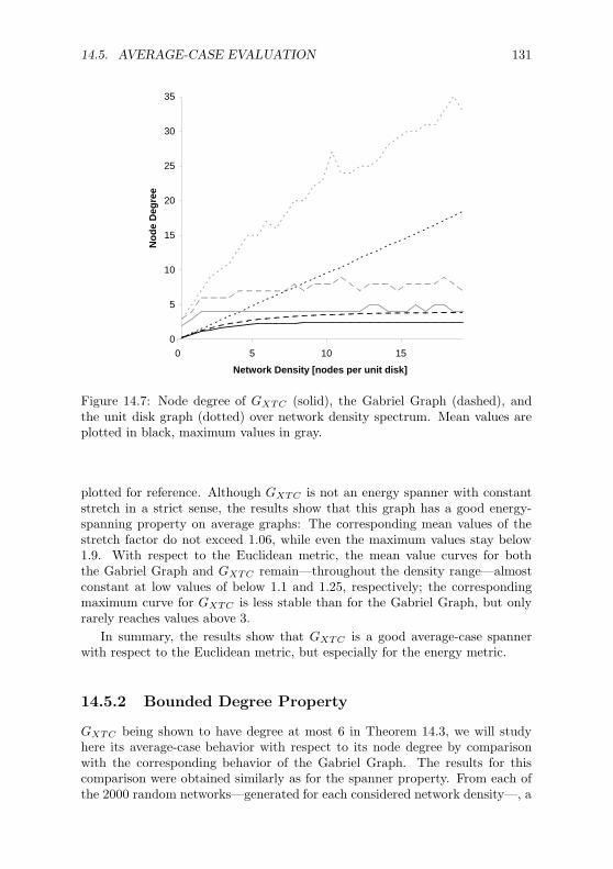
14.5. AVERAGE-CASE EVALUATION 131

0

5

10

15

20

25

30

35

0 5 10 15


No

de

Deg

ree

Figure 14.7: Node degree of GXTC (solid), the Gabriel Graph (dashed), andthe unit disk graph (dotted) over network density spectrum. Mean values areplotted in black, maximum values in gray.

plotted for reference. Although GXTC is not an energy spanner with constantstretch in a strict sense, the results show that this graph has a good energy-spanning property on average graphs: The corresponding mean values of thestretch factor do not exceed 1.06, while even the maximum values stay below1.9. With respect to the Euclidean metric, the mean value curves for boththe Gabriel Graph and GXTC remain—throughout the density range—almostconstant at low values of below 1.1 and 1.25, respectively; the correspondingmaximum curve for GXTC is less stable than for the Gabriel Graph, but onlyrarely reaches values above 3.

In summary, the results show that GXTC is a good average-case spannerwith respect to the Euclidean metric, but especially for the energy metric.

14.5.2 Bounded Degree Property

GXTC being shown to have degree at most 6 in Theorem 14.3, we will studyhere its average-case behavior with respect to its node degree by comparisonwith the corresponding behavior of the Gabriel Graph. The results for thiscomparison were obtained similarly as for the spanner property. From each ofthe 2000 random networks—generated for each considered network density—, a


randomly chosen node was examined regarding its degree in the unit disk graph,the Gabriel Graph G, and GXTC .

Figure 14.7 shows the computed results. Mean and maximum degree valuesfor the unit disk graph rise in accordance with network density. The meandegree curves for GXTC and the Gabriel Graph increase slowly for very lowdensities, remain however—once beyond the critical density range—constantat approximately 2.5 and 3.9, respectively. Although inherently less stable,the maximum degree numbers for GXTC and the Gabriel Graph stay within anarrow range from 4 to 5 and between 7 and 9. The low degree values of GXTC

suggest its suitability to reduce interference in average-case ad hoc networks.

14.5.3 Performance of Geographic Routing

GXTC ’s planarity property enables it to be employed for geographic routing.We will study its influence on geographic routing again by comparison with theGabriel Graph.

For this purpose, the results were obtained by simulation of the GOAFR+

algorithm (cf. Chapter 7) on GXTC and the Gabriel Graph of 2000 randomlygenerated networks for each considered network density. As in Section 8.3,the performance measure for the algorithm A routing from a source s to adestination t on a network G (s and t having been chosen randomly from G) isdefined as

costA(G, s, t) :=sA(G, s, t)

c`(p∗` (G, s, t)),

that is the number of steps taken by the algorithm normalized by the hop lengthof the shortest path from s to t on G.

Figure 14.8 shows the typical bell-shaped characteristic of the mean algo-rithm cost curves around the critical density range (cf. Chapter 8). The criticalnetwork density range is additionally identified by the sharp increase of thenetwork connectivity rate, that is the frequency with which a randomly chosennode pair at a given network density is connected. The figure depicts that aboveall in the critical density range the performance of the GOAFR+ algorithm onGXTC is slightly worse than on the Gabriel Graph. In light of the cost curve ofthe well-known GFG/GPSR routing algorithm (see Section 8.3), however, thedegradation of GOAFR+ employed on GXTC compared to the Gabriel Graphcan be considered negligible.

14.6 Concluding Remarks

In this chapter we introduced the XTC topology control algorithm. Comparedto previous proposals for topology control, XTC has three main advantages.First, it is not only simple, but also local: Every node communicates withits neighbors in the network not more than twice. Second, unlike many othertopology control algorithms, XTC does not require the network graph to be a

14.6. CONCLUDING REMARKS 133

0

1

2

3

4

5

6

7

8

9

0 5 10 15


Mea

n A

lgo

rith

m C

ost

0

0.1

0.2

0.3

0.4

0.5

0.6

0.7

0.8

0.9

1

Fre

qu

ency

Figure 14.8: Mean cost of the GOAFR+ routing algorithm on GXTC (solid), onthe Gabriel Graph (dotted), and of the GFG/GPSR algorithm on the GabrielGraph (dashed). For reference, the network connectivity rate is plotted againstthe right y axis.

Euclidean Graph, let alone a unit disk graph. Also for the global case of the net-work graph being a general weighted graph, XTC proves correct and computes aresulting subgraph maintaining connectivity. Third, while previously proposedtopology control algorithms commonly assumed that exact node and neighborposition information is available, XTC does not require this assumption. Thealgorithm works with the general notion of a quality order over a node’s neigh-bors. Whereas correctness of the algorithm can be shown even without anystrict assumptions on this neighbor order, the resulting topology features thebounded degree property provided that the neighbor order corresponds to Eu-clidean distances and that the network is a unit disk graph. On average-caserandom unit disk graphs, the resulting graph also shows good spanner proper-ties, above all with respect to the energy metric. Being planar, the proposedtopology is finally also suitable for geographic routing.

In this introductory topology control chapter, we discussed a lightweighttopology control algorithm which tries to operate independently of unrealisticassumptions. The XTC algorithm can be considered to follow the example of“classic” topology control in that it provably features several beneficial prop-erties. In the next and subsequent chapters we will go beyond this approachand focus explicitly on one fundamental issue in wireless networks, often main-tained to be solved or at least tackled implicitly by previously proposed topologycontrol structures: interference.


Chapter 15

Does Topology Control

Reduce Interference?

I have never let my schooling interfere with my education.Mark Twain (1835–1910)

As already mentioned in the introduction of this second part of the dissertation,one very general definition of topology control is to—given a communicationnetwork—construct a subgraph with certain beneficial properties. The previouschapter forms an example of a topology control algorithm following these lines,while specially considering omission of unrealistic assumptions and simplicityof construction.

In this and the subsequent chapters we will focus on an equally popular con-ception of topology control: Very simply put, the main goal of topology controlis often understood to be reduction of energy consumed by the network nodes inorder to extend network lifetime. Since the amount of energy required to trans-mit a message increases at least quadratically with distance, it makes sense toreplace a long link by a sequence of short links. On the one hand, energy cantherefore be conserved by abandoning energy-expensive long-range connections,thereby allowing the nodes to reduce their transmission power levels. On theother hand, confining transmission ranges also reduces interference, which inturn lowers node energy consumption by reducing the number of collisions andconsequently packet retransmissions on the media access layer. Dropping com-munication links however clearly takes place at the cost of network connectivity:If too many edges are abandoned, connecting paths can grow unacceptably longor the network can even become completely disconnected. As illustrated in Fig-ure 15.1, topology control can therefore be considered a trade-off between energyconservation and interference reduction on the one hand and connectivity onthe other hand.

136 CHAPTER 15. TOPOLOGY CONTROL AND INTERFERENCE

Topology ControlConserve Energy

Reduce Interference

Network Connectivity

Spanner Property

Figure 15.1: Topology control constitutes a trade-off between node energy con-servation and network connectivity.

The interference aspect is often maintained by developers of topology con-trol algorithms to be solved by sparseness or low node degree of the resultingtopology graph, without providing rigorous justification or proofs. The foremostcontribution of this chapter is to disprove this assertion.

In contrast to most of the related work—where the interference issue is seem-ingly solved by sparseness arguments—, we will start out by precisely definingour notion of interference. This definition of interference is based on the natu-ral question of how many nodes are affected by communication over a certainlink. By prohibiting specific network edges, the potential for communicationover high-interference links can then be confined.

We will employ this interference definition to formulate the trade-off betweenenergy conservation and network connectivity. In particular we will state certainrequirements that need to be met by the resulting topology. Among theserequirements are connectivity (if two nodes are—possibly indirectly—connectedin the given network, they should also be connected in the resulting topology)and the constant-stretch spanner property (the shortest path between any pairof nodes on the resulting topology should be longer at most by a constant factorthan the shortest path connecting the same pair of nodes in the given network).After stating such requirements, an optimization problem can be formulated tofind the topology meeting the given requirements with minimum interference.

For the requirement that the resulting topology retain connectivity of thegiven network, we will show that most of the currently proposed topology con-trol algorithms—already by having every node connect to its nearest neighbor—commit a substantial mistake: Although certain proposed topologies are guar-anteed to have low degree yielding a sparse graph, interference becomes asymp-totically incomparable with the interference-minimal topology. We will alsoshow that there exist graphs for which no local algorithm can approximatethe optimum. With respect to the sometimes desirable requirement that theresulting topology should be planar, we will show that planarity can increaseinterference.

Furthermore we will propose a centralized algorithm (LIFE) that computesan interference-minimal connectivity-preserving topology. For the requirementthat the resulting topology be a spanner with a given stretch factor, we willpresent (based on a centralized variant of the algorithm) a distributed local al-gorithm (LLISE) that computes a provably interference-optimal spanner topol-ogy.

15.1. MODEL 137

Our results are not confined to worst-case considerations; we will also showby simulation that on average-case graphs traditional topology control algorithms—in particular the Gabriel Graph and the Relative Neighborhood Graph—fail toeffectively reduce interference. Moreover, we will show that these constructionsare outperformed by the LLISE algorithm, which therefore appears average-caseeffective in addition to its worst-case optimality.

In the following section we will introduce the interference model discussedin this chapter. Focusing on the drawbacks of currently proposed topologycontrol algorithms with respect to interference in Section 15.2, we will presentinterference-optimal algorithms in the subsequent section. Section 15.4 willassess our algorithms as well as previously proposed topologies regarding theirinterference on average-case graphs.

15.1 Model

As in several previous places in this dissertation, an ad hoc network is modeledas a graph G = (V, E) consisting of a set of nodes V ⊂ R2 in the Euclidean planeand a set of edges E ⊆ V 2. Nodes represent mobile hosts, whereas edges standfor links between nodes. In order to prevent already basic communication be-tween directly neighboring nodes from becoming unacceptably cumbersome [92],it is required that a message sent over a link can be acknowledged by sendinga corresponding message over the same link in the opposite direction. In otherwords, only undirected (symmetric) edges are considered.

We assume that a node can adjust its transmission power to any valuebetween zero and its maximum power level. The maximum power levels arenot assumed to be equal for all nodes. An edge (u, v) may exist only if bothincident nodes are capable of sending a message over (u, v), in particular if themaximum transmission radius of both u and v is at least |uv|, their Euclideandistance. A pair of nodes u, v is considered connectable in the given networkif there exists a path connecting u and v provided that all transmission radiiare set to their respective maximum values. The task of a topology controlalgorithm is then to compute a subgraph of the given network graph with certainproperties, reducing the transmission power levels and thereby attempting tolower interference and energy consumption.

With a chosen transmission radius—for instance to reach a node v—a nodeu affects at least all nodes located within the circle centered at u and with radius|uv|. D(u, r) denoting the disk centered at node u with radius r and requiringedge symmetry, we consequently define the coverage of an (undirected) edge


Figure 15.2: Nodes covered by a communication link.

e = (u, v) to be the cardinality of the set of nodes covered by the disks1 inducedby u and v:

Cov(e) :=∣∣w ∈ V |w is covered by D(u, |uv|)∪

w ∈ V |w is covered by D(v, |vu|)∣∣.

In other words, the coverage Cov(e) represents the number of network nodesaffected by nodes u and v communicating with their transmission powers chosensuch that they exactly reach each other (cf. Figure 15.2).

The edge level interference defined so far is now extended to a graph inter-ference measure as the maximum coverage occurring in a graph:

Definition 15.1. The interference of a graph G=(V,E) is defined as

I(G) := maxe∈E

Cov(e).

Since interference reduction per se would be senseless (if all nodes simply settheir transmission power to zero, interference will be reduced to a minimum),the formulation of additional requirements to be met by a resulting topology isnecessary. A resulting topology can for instance be required

- to maintain connectivity of the given communication graph (if a pair ofnodes is connectable in the given network, it should also be connected inthe resulting topology graph),

1The results of this chapter can also be adapted to the case where transmission rangesare not perfect circles centered at the sending node. We adhere to this simplified model forclarity of representation.

15.2. INTERFERENCE IN KNOWN TOPOLOGIES 139

Figure 15.3: Low degree does not guarantee low interference.

- to be a spanner with constant stretch of the underlying graph (the shortestpath connecting a pair of nodes u, v on the resulting topology is longerby a constant factor only than the shortest path between u and v on thegiven network), or

- to be planar (no two edges in the resulting graph intersect).

Finding a resulting topology which meets one or a combination of such require-ments with minimum interference constitutes an optimization problem.

15.2 Interference in Known Topologies

It is often argued that sparse topologies with small or bounded degree are wellsuited to minimize interference. In this section we will show that low degree doesnot necessarily imply low interference. Moreover, we will demonstrate that mostof the currently known topology control algorithms can perform badly comparedto the interference optimum, that is a topology which minimizes interference inthe first place.

In particular, we will consider in this section the basic problem of construct-ing an interference-minimal topology maintaining connectivity of the given net-work.

The following basic observation states that—although often maintained—low degree alone does not guarantee low interference. Figure 15.3, for instance,shows a topology graph with degree 2 whose interference is however roughlyn, the number of network nodes. A node can interfere with other nodes thatare not direct neighbors in the chosen topology graph. Whereas the maximumdegree of the underlying communication graph of the given network (with all


i + 1i

2i

Figure 15.4: Exponential node chain with interference Ω(n).

nodes transmitting at full power) is an upper bound for interference, the degreeof a resulting topology graph is only a lower bound.

There exist instances where also the optimum exhibits interference Ω(n), forinstance a chain of nodes with exponentially growing distances (cf. Figure 15.4,proposed in [74]), whose large interference is caused as a consequence of the re-quirement that the resulting topology is to be connected. Every node ui (exceptfor the leftmost) is required to have an incident edge, which covers all nodesleft of ui. Assessing the interference quality of a topology control algorithmtherefore implies its interference on a given network needs to be compared tothe optimum interference topology for the same network.

To the best of our knowledge, all currently known topology control algo-rithms constructing only symmetric connections have in common that everynode establishes a symmetric connection to at least its nearest neighbor. Inother words, all these topologies contain the Nearest Neighbor Forest con-structed on the given network. In the following we will show that owing tothe inclusion of the Nearest Neighbor Forest as a subgraph, the interference ofa resulting topology can become incomparably bad with respect to a topologywith optimum interference.

Theorem 15.1. No currently proposed topology control algorithm establish-ing only symmetric connections—required to maintain connectivity of the givennetwork—is guaranteed to yield a nontrivial interference approximation of theoptimum solution. In particular, interference of any proposed topology can beΩ(n) times larger than the interference of the optimum connected topology,where n is the total number of network nodes.

Proof. Figure 15.5 depicts an extension of the example graph shown in Fig-ure 15.4. In addition to a horizontal exponential node chain, each of these nodeshi has a corresponding node vi vertically displaced by a little more than hi’sdistance to its left neighbor. If di denotes this vertical distance, the inequalitydi > 2i−1 holds. These additional nodes form a second (diagonal) exponentialline. Between two of these diagonal nodes vi−1 and vi, an additional helpernode ti is placed such that |hi, ti| > |hi, vi|.

The Nearest Neighbor Forest for this given network (with the additionalassumption that the transmission radius of each node can be chosen sufficiently


hi

vi

di

ti

vi−1

Figure 15.5: Two exponential node chains.

Figure 15.6: The Nearest Neighbor Forest yields interferenceΩ(n).

Figure 15.7: Optimal tree with constant interference.


u v

Figure 15.8: Worst-case graph for which no local algorithm can approximateoptimum interference.

large) is shown in Figure 15.6. Roughly one third of all nodes being part ofthe horizontally connected exponential chain, interference of any topology con-taining the Nearest Neighbor Forest amounts to at least Ω(n). An interference-optimal topology, however, would connect the nodes as depicted in Figure 15.7with constant interference.

In other words, already by having each node connect to the nearest neigh-bor, a topology control algorithm makes an “irrevocable” error. Moreover, itcommits an asymptotically worst possible error since the interference in anynetwork cannot become larger than n.

As roughly one third of all nodes are part of the horizontal exponential nodechain in Figure 15.5, the observation stated in Theorem 15.1 would also holdfor an average interference measure, averaging interference over all edges.

The following theorem even shows that for connectivity-preserving topolo-gies no local algorithm can approximate optimum interference for every givennetwork. Thereby the definition of a distributed local algorithm assumes thateach network node is informed about its network neighborhood only up to agiven constant distance.

Theorem 15.2. For the requirement of maintaining connectivity of the givennetwork, there exists a class of graphs for which no local algorithm can approx-imate optimum interference.

Proof. In Figure 15.8 the maximum transmission radius of a node is |uv|. nbeing the number of nodes in the graph, let the shaded area contain Ω(n)evenly distributed nodes which can be connected with constant interference.For each such node w, the inequalities |wv| < |uv| and |uw| > |uv| hold. It

15.3. LOW-INTERFERENCE TOPOLOGIES 143

follows that the edge (u, v) has interference in Ω(n) since it covers all nodes inthe shaded area. In addition, there is a chain of nodes (dashed path) connectingnode u with node v indirectly through the nodes located in the shaded area.The nodes in the chain are located in such a way that it is possible to connectthem with constant interference. For such a graph, O(1) interference can beachieved by connecting u to the rest of the graph through the chain of nodesand not directly through edge (u, v), which would cause Ω(n) interference.

A local algorithm at node u has to decide if it can drop edge (u, v). This isonly possible if u knows about the existence of an alternative path from u to vin order to maintain connectivity. By elongating the chain sufficiently, the localalgorithm can thus be forced to include edge (u, v), pushing up interference toO(n) whereas the optimum is Ω(1).

As mentioned in Section 15.1, another popular requirement for topologycontrol algorithms besides bounded degree is planarity of the resulting topology,meaning that no two edges of the resulting graph intersect. This is often desiredfor the application of geographic routing algorithms that are only applicable toplanar graphs. But topology control algorithms enforcing planarity are notoptimal in terms of interference:

Theorem 15.3. There exist graphs on which interference-optimal topologies—required to maintain connectivity—are not planar.

Proof. In Figure 15.9, the maximum transmission radius of a node is |ab|. Alleligible edges are depicted together with the coverage areas for the edges whoseincident nodes are both in a, b, c, d. The indicated weight of an edge e cor-responds to its coverage Cov(e). V and W represent sets of 3 and 4 nodes,respectively, which can be connected among themselves with interference 3. Atopology control algorithm can only reduce interference by removing all edgeswith maximum interference (here (a, c) and (b, c)) from the graph. Thereafter,no further edge can be removed without breaking connectivity since the graphwithout (a, c) and (b, c) is a tree. Thus, the resulting tree is interference-optimaland non-planar, as both edges (a, b) and (c, d) have to remain in the resultingtopology.

15.3 Low-Interference Topologies

In this section we will present three algorithms that explicitly reduce interferenceof a given network. The first algorithm is capable of finding an interference-optimal topology maintaining connectivity of the given network. The othertwo algorithms compute an interference-optimal topology under the additionalrequirement of constructing a spanner of the given network. Whereas the firstspanner algorithm assumes global knowledge of the network, the second can becomputed locally.


V

9

4 nodes

3 nodes

4

8

5

3

2

d

b

c u

9

8a

W

Figure 15.9: Node set whose interference-optimal topology is not planar.

15.3.1 Interference-Optimal Spanning Forest

In the following we again require the resulting topology to maintain con-nectivity of the given network. A topology graph meeting this requirement cantherefore consist of a tree for each connected component of the given networksince additional edges do not contribute to graph connectivity while poten-tially unnecessarily increasing interference. A Minimum Interference Forest istherefore a set of trees maintaining the connectivity of the given network withleast possible interference. As the following theorem shows, the LIFE algorithmcomputes such a forest.

Theorem 15.4. The forest constructed by LIFE is a Minimum InterferenceForest.

Proof. The LIFE algorithm computes a minimum spanning forest (MSF) of thegraph G = (V, E), where E is the set of all eligible edges, if every edge e ∈ E isattributed the weight Cov(e). With its greedy strategy, it follows the lines ofKruskal’s MSF algorithm [26]. To prove the theorem, it is therefore sufficientto show that the MSF is optimal with respect to interference. Optimality ofLIFE then follows from the fact that a minimum spanning forest also minimizesthe maximum edge weight in any spanning forest. (Assuming for contradictionthat G∗ is an MSF with maximum weight edge e∗, whereas GLIFE is a spanningforest with lower maximum edge weight, e∗ could be replaced by a corresponding


Low Interference Forest Establisher (LIFE)

Input: a set of nodes V , each v ∈ V having attributed a maximum transmissionradius rmax

v

1: E = all eligible edges (u, v) (rmaxu ≥ |uv| and rmax

v ≥ |uv|)// E will contain all unprocessed edges

2: ELIFE = ∅3: GLIFE = (V, ELIFE)4: while E 6= ∅ do5: e = (u, v) ∈ E with minimum coverage6: if u, v are not connected in GLIFE then7: ELIFE = ELIFE ∪ e8: end if9: E = E \ e

10: end whileOutput: Graph GLIFE

edge from GLIFE , yielding a spanning forest with total edge weight smaller thanG∗’s, which contradicts the assumption that G∗ is an MSF.)

With an appropriate implementation of the connectivity query in Line 6, therunning time of the algorithm LIFE is O

(n2 log n

). If the given network is known

to consist of only one connected component, Prim’s minimum-spanning-treealgorithm can be employed with running time O

(n2). Algorithms computing

a minimum spanning tree in a distributed way—as particularly suitable for adhoc networks—are described in detail in [86].

15.3.2 Low-Interference Spanners

LIFE optimizes interference for the requirement that the resulting topology hasto maintain connectivity. In addition to connectivity it is often desired thatthe resulting topology should be a spanner with constant stretch of the givennetwork. A spanner with stretch factor t can be formally defined as follows:

Definition 15.2 (t-Spanner). A t-spanner of a graph G = (V, E) is a subgraphG′ = (V, E′) such that for each pair (u, v) of nodes c(p∗

G′(u, v)) ≤ t · c(p∗G(u, v)),where c(p∗G′(u, v)) and c(p∗G(u, v)) denote the length of the shortest path betweenu and v in G′ and G, respectively.

In this chapter we consider Euclidean spanners, that is, the length of a path isdefined as the sum of the Euclidean lengths of all its edges (cf. Chapter 3). Withslight modifications, our results are however also extendable to hop spanners,where the length of a path corresponds to the number of its edges.

Algorithm LISE is a topology control algorithm that constructs a t-spannerwith optimum interference. LISE starts with a graph GLISE = (V, ELISE)where ELISE is initially the empty set. It processes all eligible edges of the


Low Interference Spanner Establisher (LISE)

Input: a set of nodes V , each v ∈ V having attributed a maximum transmissionradius rmax

v ; a stretch factor t ≥ 11: E = all eligible edges (u, v) (rmax

u ≥ |uv| and rmaxv ≥ |uv|)

// E will contain all unprocessed edges2: ELISE = ∅3: GLISE = (V, ELISE)4: while E 6= ∅ do5: e = (u, v) ∈ E with maximum coverage6: while c(p∗(u, v) in GLISE) > t |uv| do7: f = edge ∈ E with minimum coverage8: move all edges ∈ E with coverage Cov(f) to ELISE

9: end while10: E = E \ e11: end whileOutput: Graph GLISE

given network G = (V, E) in descending order of their coverage. For each edge(u, v) ∈ E not already in ELISE , LISE checks whether there exists a path fromu to v in GLISE with Euclidean length at most t |uv|. As long as no suchpath exists, the algorithm keeps inserting all unprocessed eligible edges withminimum coverage into ELISE .

To prove the interference optimality of GLISE , we introduce an additionallemma, which shows that GLISE contains all eligible edges whose coverage isless than I(GLISE).

Lemma 15.5. The graph GLISE = (V, ELISE) constructed by LISE from agiven network G = (V, E) contains all edges e in E whose coverage Cov(e) isless than I(GLISE).

Proof. We assume for the sake of contradiction that there exists an edge e in Ewith Cov(e) < I(GLISE) which is not contained in ELISE . Consequently, LISEnever takes an edge with coverage Cov(e) in Line 7 since the algorithm wouldinsert all edges with Cov(e) into ELISE in Line 8 instantly (thus also e). Thereexists however an edge f in ELISE with Cov(f) = I(GLISE) eventually takenin Line 7. Therefore the inequality Cov(e) < Cov(f) holds. At the time thealgorithm takes f in Line 7, all edges taken in Line 5 must have had coveragegreater than or equal to Cov(f) since the maximum of an ordered set can onlybe greater than or equal to the minimum of the same set. Hence e has neverbeen taken in Line 5 and therefore has never been removed from E in Line 10.Consequently, e is still in E when f is taken as the edge with minimum coveragein E. Thus Cov(f) ≤ Cov(e) holds, which leads to a contradiction.

With Lemma 15.5 we are ready to prove that the resulting topology con-structed by LISE is an interference-optimal t-spanner.


Theorem 15.6. The graph GLISE = (V, ELISE) constructed by LISE from agiven network G = (V, E) is an interference-optimal t-spanner of G.

Proof. In order to show that GLISE meets the spanner property, it is sufficientto prove that for each edge (u, v) ∈ E there exists a path in GLISE with lengthnot greater than t |uv|. This holds since for a shortest path p∗(u, v) in G apath p′(u, v) in GLISE with c(p′) ≤ t c(p) can be constructed by substitutingfor each edge on p the corresponding spanner path in GLISE. For edges in Ewhich also occur in ELISE , the spanner property is trivially true. On the otherhand an edge (u, v) can only be in E but not in ELISE if a path from u to vin GLISE with length not greater than t |uv| exists (see if-condition in Line 6).Thus, GLISE is a t-spanner of G.

Interference optimality of LISE can be proved by contradiction. We thereforassume, that GLISE is not an interference-optimal t-spanner. Let G∗ = (V, E∗)be an interference-optimal t-spanner for G. Since GLISE is not optimal, itfollows that I(GLISE) > I(G∗). Thus all edges in E∗ have coverage strictly lessthan I(GLISE). It follows from Lemma 15.5 that E∗ is a nontrivial subset ofELISE. Let T be the set of edges in ELISE with coverage I(GLISE) and letG = (V, E) be the graph with E = ELISE \ T . G is a t-spanner since E∗ isstill a subset of E, and I(G) ≤ I(GLISE) − 1 holds. Because T is eventuallyinserted into ELISE in Line 8, there exists an edge (u, v) ∈ E that was taken inLine 5 and for which no path p(u, v) exists in G with c(p) ≤ t |uv|. Thus, G isno t-spanner (and therefore neither G∗), which contradicts the assumption thatG∗ is an interference-optimal t-spanner.

As regards the running time of LISE, it computes for each edge at mostone shortest path. This holds since multiple shortest path computations for thesame edge in Line 6 cause at least as many edges to be inserted into ELISE

in Line 8 without computing shortest paths for them. Since finding a shortestalternative path for an edge requires O

(n2)

time and as the network containsat most the same amount of edges, the overall running time of LISE is as wellpolynomial in the number of network nodes.

In contrast to the problem of finding a connected topology with optimuminterference, the problem of finding an interference-optimal t-spanner is locallysolvable. The reason for this is that finding an interference-optimal path p(u, v)for an edge (u, v) with c(p) ≤ t |uv| can be restricted to a certain neighborhoodof (u, v).

In the following we will describe a local algorithm similar to LISE that isexecuted at all eligible edges of the given network. In reality, algorithm LLISE(Local LISE) is executed for each edge by one of its incident nodes (for instancethe one with the greater identifier). The description of LLISE assumes the pointof view of an edge e = (u, v). The algorithm consists of three main steps:

1) Collect ( t2 )-neighborhood,

2) compute minimum interference path for e, and


LLISE

1: collect ( t2 )-neighborhood GN = (VN , EN ) of G = (V, E)

2: E′ = ∅3: G′ = (VN , E′)4: repeat5: f = edge ∈ EN with minimum coverage6: move all edges ∈ EN with coverage Cov(f) to E ′

7: p = shortestPath(u− v) in G′

8: until c(p) ≤ t |uv|9: inform all edges on p to remain in the resulting topology.

Note: GLL = (V, ELL) consists of all edges eventually informed to remainin the resulting topology.

3) inform all edges on that path to remain in the resulting topology.

In the first step, e gains knowledge of its ( t2 )-neighborhood. For a Euclidean

spanner, the k-neighborhood of e is defined as all edges that can be reached (ormore precisely at least one of their incident nodes) over a path p starting at uor v, respectively, with c(p) ≤ k c(e). Knowledge of the ( t

2 )-neighborhood at alledges can be achieved by local flooding (cf. Chapter 10).

Theorem 15.7. The graph GLL = (V, ELL) constructed by LLISE from a givennetwork G = (V, E) is an interference-optimal t-spanner of G.

During the second step, a minimum-interference path p from u to v withc(p) ≤ t c(e) is computed. LLISE starts with a graph GLL = (V, ELL) consistingof all nodes in the ( t

2 )-neighborhood and an initially empty edge set. It insertsedges consecutively into ELL—in ascending order according to their coverage—,until a shortest path p∗(u, v) is found in GLL with c(p∗) ≤ t c(e).

In the third step, e informs all edges on the path found in the second stepto remain in the resulting topology. The resulting topology then consists of alledges receiving a corresponding message. In the following we will show thatit is sufficient for e to limit the search for an interference-optimal path p(u, v)meeting the spanner property to the ( t

2 )-neighborhood of e.

Lemma 15.8. Given an edge e = (u, v), no path p from u to v with c(p) ≤ t c(e)contains an edge which is not in the ( t

2 )-neighborhood of e.

Proof. For the sake of contradiction we assume that a path p from u to v withc(p) ≤ t c(e) contains at least one edge (w, x) not in the ( t

2 )-neighborhood of e.Without loss of generality we further assume that, traversing p from u to v, wevisit w before x. Since (w, x) is not in the ( t

2 )-neighborhood, by definition, nopath from u to w with length less than or equal to ( t

2 )|e| exists (the same holdsfor any path from v to x). Consequently, the inequality c(p) > t c(e) + |wx|holds, which contradicts the assumption that c(p) ≤ t c(e).

15.4. AVERAGE-CASE INTERFERENCE 149

With Lemma 15.8 we are now able to prove that the topology constructedby LLISE is a t-spanner with optimum interference.

Proof. The spanner property of LLISE can be proved similar to the first partof the proof of Theorem 15.6, where LISE is shown to be a t-spanner.

In order to show interference optimality, it is sufficient to prove that thespanner path constructed for any edge e = (u, v) ∈ G by LLISE is interference-optimal, where interference of a path is defined as the maximum interferenceof an edge on that path. The reason for this is that only edges that lie onone of these paths remain in the resulting topology; non-optimality of GLL

would therefore imply non-optimality of at least one of these spanner paths.In the following we look at the algorithm executed by e = (u, v). In Line 6,edges in E are consecutively inserted into E ′, starting with E′ = ∅, until aspanner path p from u to v is found in Line 8. Since LLISE inserts the edgesinto E′ in ascending order according to their coverage and since p is the firstpath meeting the spanner property, p is an interference-optimal t-spanner pathfrom u to v in the ( t

2 )-neighborhood. From Lemma 15.8 we know that the( t2 )-neighborhood of e contains all spanner paths from u to v and therefore also

the interference-optimal one. Thus it is not possible that LLISE does not seethe global interference-optimal t-spanner path due to its local knowledge aboutG. Consequently, p is the global interference-optimal t-spanner path of e.

15.4 Average-Case Interference

In this section we will consider interference of topology control algorithms inaverage-case graphs, that is in graphs with randomly placed nodes.

In particular, networks were constructed by placing nodes randomly anduniformly on a square field of size 20 by 20 units and subsequently computingfor each node set the unit disk graph (cf. Definition 3.1). The resulting unit diskgraphs were then employed as input networks for topology control. Since nodedensity is a fundamental property of networks with randomly placed nodes, thenetworks were generated over a spectrum of node densities.

15.4.1 Connectivity-Preserving Topologies

To evaluate connectivity-preserving topologies on average-case graphs, two well-known topology control structures are considered, in particular the GabrielGraph [38] and the Relative Neighborhood Graph [102]. The interference-reducing effect of these two constructions is considered by comparison withthe interference value of the given unit disk graph network on the one handand with the interference-optimal connectivity-preserving topology on the otherhand. The interference-optimal topology was constructed by means of the LIFEalgorithm presented in Section 15.3.


0

10

20

30

40

50

60

70

80

90

0 5 10 15 20 25 30 35 40


Inte

rfer

ence

Figure 15.10: Interference values of the unit disk graph without topology control(dotted), the Gabriel Graph (dash-dotted), the Relative Neighborhood Graph(dashed), and the interference-optimal connectivity-preserving topology (solid).

Figure 15.10 shows the interference mean values over 1000 networks for eachsimulated network density. While the resulting interference curves behave sim-ilarly for very low network densities, they fall into three groups with increasingdensity: At a density of roughly 5 network nodes per unit disk, the interference-optimal curve levels off and remains at a value of approximately 11.5. On theother hand the interference curve of the unit disk graph without topology controlrises almost linearly. Between these two extremes the Gabriel Graph and Rela-tive Neighborhood Graph values increase clearly more slowly than the unit diskgraph curve, but show significantly higher values than the interference-optimaltopology.

The simulation results show that the edge reduction performed by the GabrielGraph and Relative Neighborhood Graph constructions reduce interference ofthe given network; this effect is clearer with the Relative Neighborhood Graphdue to its stricter edge inclusion criterion and consequently its being a sub-graph of the Gabriel Graph (see also Figure 14.4). However, the interferencevalues of these two constructions are considerably higher than the results of theinterference-optimal connectivity-preserving topology. Furthermore, although(unless in special cases) the Relative Neighborhood Graph has degree at most6, it is not even clear whether with increasing network density the respectiveinterference curve remains around the maximum value found so far or whetherit would increase further for densities beyond the simulated spectrum. It can

15.4. AVERAGE-CASE INTERFERENCE 151

0

5

10

15

20

25

0 5 10 15


Inte

rfer

ence

Figure 15.11: Interference values of LLISE for stretch factors 2 (dotted), 4 (dash-dot-dotted), 6 (dash-dotted), 8 (dashed), and 10 (solid). Interference values ofthe Relative Neighborhood Graph (upper gray) and the interference-optimalconnectivity-preserving topology (lower gray) are plotted for reference.

therefore be concluded that also for average-case graphs sparseness does notimply low interference.

15.4.2 Low Interference Spanners

Going beyond connectivity-preserving topologies, we will consider in this sec-tion constant-stretch spanners, that is topologies guaranteeing that the shortestpaths on the resulting topology are only by a constant factor longer than onthe given network (cf. Section 15.3.2).

Figure 15.11 depicts simulation results—in particular the mean interferencevalues over 100 networks at each simulated network density—of the topologyconstructed by the LLISE algorithm introduced in Section 15.3 for differentstretch factors t. The simulation results show that by increasing the requestedstretch factor it is possible to achieve interference values close to the optimuminterference values caused by connectivity-preserving topologies as described inthe previous section. Moreover, even with a low stretch factor of 2, LLISEdoes not perform worse than the Relative Neighborhood Graph, which is nota constant-stretch spanner. In summary, the simulation results show that theLLISE algorithm performs well with respect to interference also on average-casegraphs. An illustration of the simulation graphs is provided in Figure 15.12.


Figure 15.12: The unit disk graph G (top left, interference 50), the RelativeNeighborhood Graph of G (top right, interference 25), GLL computed by LLISEwith stretch factors 2 (bottom left, interference 23) and 10 (bottom right, in-terference 12) at a network density of 20 nodes per unit disk on a square fieldof 10 units side length. Note that, for instance in the western region of thegraph, LLISE—depending on the chosen stretch factor—omits high-interference“bridge” edges if alternative spanning paths exist.



In this chapter we disprove the widely advocated assumption that sparse topolo-gies automatically imply low interference. In contrast to most of the relatedwork we provide an intuitive definition of interference. With this interfer-ence model we show that currently proposed topology control constructions—although claiming so—do not in the first place focus on reducing interference.

In addition, we propose provably interference-minimal connectivity-preservingand spanner constructions. A locally computable version of the interference-minimal spanner construction can even be considered practicable since it isshown to significantly outperform previously suggested topology control algo-rithms also on average-case graphs.

As important as an explicit definition of interference is for its analysis, aclear drawback of the definition presented in this chapter is that it assumes theperspective of the sender of a message. Formally, this notion is reflected by thedefinition of the coverage of an edge, which counts the number of network nodesaffected by communication over the considered edge. This stands in oppositionto the fact that signal disturbance and message collisions actually occur atthe intended receiver of a message. This characteristic of interference forms thecore of the following chapters discussing approaches to model interference whichassume the signal receiver’s perspective.


Chapter 16

Receiver-Centric

Interference in Sensor

Networks

When a book and a head collide and there is a hollow sound,is it always from the book?

Georg Christoph Lichtenberg (1742–1799)

The previous chapter states two main points. First, an implicit notion ofinterference—as advocated by most of the previous work—can lead to topol-ogy control algorithms that fail to effectively reduce interference. Second, itintroduces an explicit definition of interference, based on the number of nodespotentially disturbed by communication over a link.

In contrast to this approach, we will assume in this chapter a receiver-centric perspective. Particularly, we will formulate an interference definitionat the heart of which lies the question by how many other nodes a givennetwork node can be disturbed. Compared to the sender-centric interferencedefinition proposed in the previous chapter, the definition of interference pre-sented in this chapter reflects intuition more closely in the sense that inter-ference is considered at the receiver, where message collisions prevent properreception. Informally, our interference definition can also be considered to cor-respond to the effort required to avoid collisions, be it by means of time divisionmultiplexing—assigning transmission time slots such that no two messages col-lide at a receiving node—, by means of frequency division multiplexing—havingmessages sent in different assigned frequency bands—, or by means of code divi-sion multiplexing—where small interference allows for reduced coding overhead.

In this chapter, we will consider interference in sensor networks. A sensornetwork consists of sensors deployed in a given region with the task of sensing a

156 CHAPTER 16. INTERFERENCE IN SENSOR NETWORKS

certain physical value (such as temperature, humidity, brightness, or motion).The sensors are equipped with radio devices and—in the popular monitoringscenario model—periodically transfer the sensed data to a designated data sinknode. To allow all data to be gathered at the sink, a topology control algorithmtherefore constructs a sink tree, a directed tree with all arcs (directed edges)—modeling unidirectional communication links—pointing towards the sink node.In the context of interference reduction, the task of the topology control algo-rithm is to find such a sink tree with least possible interference. Thereby weaccount for the fact that in the monitoring scenario, communication from thesink to the sensors occurs rarely and can therefore be neglected with respect tointerference.

Assuming a worst-case perspective, we will show that there are networkinstances in which any topology control algorithm will construct a resultingnetwork with interference at least log n− 1. We furthermore propose the Near-est Component Connector (NCC) algorithm, which provably produces at mostO(log n) interference in any network in polynomial time. In this sense, the NCCalgorithm is asymptotically optimal. In a second part of this chapter we willcompare the NCC algorithm with previously proposed structures in averagenetworks. On the one hand we will show that—besides being asymptoticallyworst-case optimal—NCC also in the average case produces interference re-sults comparable with previously proposed structures. On the other hand, aminimum-spanning-tree-based structure not originally designed to reduce in-terference interestingly appears to outperform NCC in average-case networks,while it cannot guarantee to produce low interference in worst-case examples.

The chapter is organized as follows: We will first introduce our receiver-centric interference model and a formulation of the considered interference min-imization problem in the following section. While Section 16.2 shows that thereexist network instances in which any topology control algorithm will produceinterference at least log n − 1, the subsequent section presents the NCC algo-rithm and proves that it matches this lower bound. Section 16.4 finally discussesinterference generated by NCC and other algorithms in average-case networks.

16.1 Model and Notation

In this section we will describe our model of a sensor network and formallydefine interference and interference minimization in the context of our model.

Our model of a sensor network is a directed graph G(V, E) where nodesv1, . . . , vn placed in the plane represent the set of sensors including the sink.Communication links between sensors are modeled as (directed) arcs. We as-sume that the transmission power of each node can be adjusted. Higher trans-mission power allows a node to send messages over a longer distance. Weassume that the covered area of a sending node vi is a disk with vi in its center.Furthermore we assume that a node can reach another node only if it is atmost 1 distance unit away. In other words, the graph consisting of all eligible

16.1. MODEL AND NOTATION 157

arcs if all nodes set their transmission power to the maximum possible valuescorresponds to the unit disk graph constructed given the node set V (cf. Defini-tion 3.1). Finally we only consider connectable graphs, which means that—withall transmission radii set to their maximum values—a path from any node toany other node in the network is constructible or—more technically—the unitdisk graph given the node set V consists of one connected component.

If we want to minimize interference in sensor networks, we have to lookat topologies in which each node sends its data to at most one other node,and a valid graph contains a path from every sensor to the sink. These tworequirements result in a tree with the sink as its root and all arcs pointingtowards the root. We call such a tree a sink tree. Figure 16.1 shows a samplesink tree with 6 nodes.

Definition 16.1. Given a set of nodes V and a sink s, a sink tree is a treespanning V with all arcs pointing towards s.

We use an explicit model of interference. We explicitly count the number ofnodes potentially disturbing reception of a message. This definition reflects thefact that interference is a problem occurring at the receiver. Minimizing theinterference at each possible receiver (each node in the network) reduces thenumber of potential message collisions in the network and therefore lowers theprobability of required retransmission. This approach intends to save energyand extend the lifetime of sensors equipped with batteries.

In particular, the interference value of a single node is defined to be thenumber of transmission circles by which the node is covered.

Definition 16.2. The interference value of a single node v is defined as

I(v) := |u|u 6= v ∧ v ∈ D(u, ru)|

where D(u, ru) stands for the transmission circle with node u in its center andradius ru.

The interference of a whole network is defined as the maximum of all inter-ference values in the graph (see Figure 16.1).1

Definition 16.3. The interference of a Graph G(V, E) is defined as

I(G) := maxv∈V

I(v).

The problem we study in this chapter consists in finding a sink tree withleast possible interference for a given sensor network.

1It can be argued similarly that the interference of a whole network can be defined asthe average of the node interference values. Such a definition is not considered in this chap-ter. Note that with this alternative definition of interference, the problem of finding a validdata-gathering structure with minimum interference can be solved optimally constructing aMinimum Directed Spanning Tree with arc weights corresponding to the number of nodescovered by each edge.


2

2 1

0

0

3

Figure 16.1: A sink tree with 6 nodes, the uppermost node being the sink node.Each node is labeled with its interference value. The interference of the wholenetwork is 3.

Definition 16.4. The Minimum-Interference Sink Tree (MIST) problem is de-fined as the problem of finding a sink tree for a given node set with minimalinterference.

In the remainder of this chapter we will consider topology control algorithmswith the goal of solving the MIST problem.

16.2 A Lower Bound

In this section we will show that n nodes in a sensor network can be arranged in away that there exists no algorithm able to construct a sink tree with interferenceless than log(n)− 1. The existence of such examples constitutes a lower boundwith respect to interference.

Theorem 16.1. There exist sensor networks with nodes arranged in a way thatno algorithm can construct a sink tree with interference less than log(n) − 1.

Proof. To prove this theorem, we present an arrangement of n = 2s nodes whichcannot be connected to the given sink in the described way with interferenceless than log(n)− 1. The nodes are arranged on a horizontal line, as illustratedin Figure 16.2. The first k = 4 nodes v1, v2, v3, and v4, are positioned atcoordinates 0, 1·ν, 3·ν, and 4·ν, where ν = 1/(4·3s−2) is a normalization factor.Then a copy of the already positioned nodes is placed in distance d = |v1vk| tothe right of node vk. This construction is recursively repeated until 2s nodesare placed on the horizontal line. Note that due to normalization of the nodepositions every node can reach any other node in the network.

16.3. NCC ALGORITHM 159

Figure 16.2: A recursive arrangement of 16 nodes on a horizontal line. Thelabels indicate distances without normalization by the factor 1/(4 · 3s−2).

After the execution of any possible algorithm, there has to exist a directedpath from each node in the set to the global sink. Let G1 be the node groupv1, . . . , v2s−1 and G2 := v2s−1+1, . . . , v2s. If we assume without loss of gener-ality that the node group G2 contains the global sink, the result of an algorithmhas to contain an arc from G1 to G2. According to the special arrangement ofthe nodes in our example, the gap between G1 and G2 has length equal to the(Euclidean) diameter of the two groups. The arc between G1 and G2 cannotbe shorter than this gap and therefore interferes with all nodes but one in G1.Figure 16.3 illustrates the idea of the proof.

If, in a next step, we look into G1, there are 2s−1 nodes partitioned into twosubgroups G1.1 and G1.2. Assuming, again without loss of generality, that theabove arc from G1 to G2 originates in G1.2, we can observe that there must existan arc leading out from G1.1, which—bridging G1.1’s adjacent gap—interfereswith all nodes in G1.1 (except for the node at which this arc originates). Theexistence of such an arc is a consequence of the required directed path fromeach node to the sink. The same argument recursively holds for all node levelsin the arrangement.

This all together proves that at least one node is affected on every level ofrecursion. And as the node set is of size 2s, we obtain a maximum interferenceof at least s − 1 or log(n) − 1.

16.3 NCC Algorithm

Having presented a lower bound on interference in the previous section, we willintroduce in this section the Nearest Component Connector algorithm (NCC)matching this lower bound and being described in detail in Algorithms 16.1 and16.2.

The general idea of this algorithm is to connect components to their nearestneighbors. This is done in several rounds and leads to a sink tree. A componentcan be a single node or a group of previously connected nodes. When thealgorithm starts, each node in the given sensor network forms a component ofits own. First, the predefined global sink is treated exactly as a normal node.Whenever two or more components are connected in one round, they form


Figure 16.3: Illustration of the proof of Theorem 16.1. The numbers stand forthe number of nodes in each group. The dark fields represent the unaffectednodes in the last step and the hollow node (bottom) is the one whose interferencevalue is incremented in each step.

a single component in the following round of NCC. Considering an arbitrarycomponent at any point of time of the algorithm execution, we observe thatthis component has exactly one node all other component members have adirected path to. This means that there is one node which gathers all senseddata of the component. We call this node the local sink of its component.

Whenever a new arc is established during the execution of NCC, it goes froma local sink of a component C to the nearest node not in C. However, due to thefact that all nodes have maximum transmission range 1, it is possible that thecurrent sink s of a component C cannot connect to any node outside C. In thiscase another node s′ is designated to become the new sink of C, particularlythe nearest node to s (with respect to the number of hops) capable of reachingany node outside C. This is accomplished by removing all arcs originating atnodes on the shortest path p∗(s, s′) from s to s′ and subsequently adding thearcs along p∗(s, s′) (cf. Algorithm 16.2). Note that every component containsat least one node capable of reaching another node outside its component sincewe only consider connectable networks.

If a round—connecting every sink to its nearest neighbor outside its compo-nent—produces a cycle, this cycle is broken by removing one of its arcs at theend of the round. This leads to the construction of a valid sink tree topology. Itis possible that, after the last round of NCC, the root of the resulting tree is notnecessarily the global sink. In this case, the root of the resulting tree is moved


Input: V : a set of nodes placed in the planesg ∈ V : a predefined global sink

1: G := (V, E := ∅)2: lsinks := V // set of local sinks3: while |lsinks| > 1 do4: for all s ∈ lsinks do5: E′ := ∅6: C := component containing s7: if s cannot reach any node outside C then8: s′ := nearest node to s (hop metric) capable of reaching a node

outside C9: movesink(G, s, s′)

10: s := s′

11: end if12: E′ := E′ ∪ e, where e is the arc from s to its nearest neighbor (Eu-

clidean distance) outside C13: end for14: if G′ := (V, E ∪ E′) contains cycles then15: remove one of the arcs in each cycle from E ′

16: end if17: G := G′

18: lsinks := sinks in G // sinks are nodes having no outgoing arc19: end while20: s := only remaining sink in lsinks21: if s 6= sg then22: movesink(G, s, sg)23: end ifOutput: G

Algorithm 16.1: Nearest Component Connector Algorithm NCC

Input: Graph G = (V, E)s1: a local sink in Gs2: a node in the same component as s1

1: sp := shortest path from s1 to s2 according to the hop metric2: remove all arcs originating at nodes on sp (including s2) from E3: add arcs on sp to E

Algorithm 16.2: Procedure movesink(G, s1, s2)

to the global sink again by means of the movesink procedure (Algorithm 16.2).Figure 16.4 shows a sample execution of the NCC algorithm.

We will now prove that the presented NCC algorithm constructs a validsink tree topology for a given sensor network consisting of n nodes with an


0 1

2 3

Figure 16.4: A sample execution of NCC on a given set of 5 nodes. Situation 0shows the given nodes and the predefined sink (top right node) In each of thefollowing two rounds, every local sink connects to the nearest node not in itsown component. In Round 2, a cycle is produced. It is broken at the end ofthe round by removing one of the involved arcs (dashed arrow). After the lastround (Situation 3) the arc originating from the global sink is removed and anarc is added from the only remaining local sink to the predefined global sink.For clarity of representation, the node distances are assumed to be sufficientlysmall such that execution of the movesink procedure is not required.

interference value in O(log n). We will also see that the execution of NCC takespolynomial time only.

Theorem 16.2. The NCC Algorithm constructs a sink tree on a given GraphG = (V, E) with |V | = n producing an interference value of at most O(log n) inpolynomial time.

Proof. This proof has three parts. In the first part we show that NCC does notneed more than log n rounds (while-loop iterations) to build the sink tree. Inthe second part we show that in each of these rounds the interference value of anode will not be incremented by more than a constant value. In part three weshow that NCC terminates in time polynomial in the total number of nodes.

To show the first part, we use the fact that in each round a local sink seither establishes an arc to the nearest node of another component or thatanother component establishes an arc to the component s is part of. The twoor more connected components together form one component in the next round.Therefore the number of components in round i is at most half the number of


Ci

li

vj livj

> livj

Figure 16.5: An illustration of the second part of the proof of Theorem 16.2. Anarc from the local sink li to vj only interferes with nodes in li’s component andvj (and nodes in other components only if they are exactly at distance livj).

the components in round i − 1. This implies that after at most log n roundsonly one component is left and the algorithm terminates.

In the second part of the proof we show that each round increases the in-terference value at most by a constant. First, the movesink(G, s, s′) procedureonly increases the interference values of nodes in C, the component of s and s′,since none of the nodes on the shortest path from s to s′ can reach any nodeoutside C; furthermore, introduction of the arcs on the shortest path from s tos′ increases the interference value by at most 3. (A node v suffering interferenceincrease of at least 4 would contradict the fact that only arcs on a shortest pathare added to the graph; the shortest path could be shortcut via v, exploitingthat in the unit disk graph model all arcs of length up to one unit are eligible.)Second, once the sink of a component C can reach another node outside C, weuse the fact that each sink connects to the nearest node in a component differentfrom its own, as illustrated in Figure 16.5. If a local sink li being contained incomponent Ci connects to a node vj , its distances from all nodes not in Ci are atleast |livj |. Therefore only nodes which are members of component Ci or nodeswith the same distance from li as vj are affected by the new arc. Furthermore,a component establishes at most one new arc in a single round and maximally6 local sinks can establish an arc to the same node.2 All this shows that theinterference value of a node is incremented at most by a constant in a singleround of NCC.

2This is the so-called “kissing number.” It is defined as the number of equivalent spheresthat touch an equivalent sphere without intersections. The kissing number in the two-dimensional plane is 6. In three dimensions it is 12.


Together with part one of the proof and the fact that the movesink pro-cedure is applied at most one more time, it follows that the interference valueof any node is incremented at most log(n) + 1 times and each time by at mosta constant value. This proves that the interference of the whole network is inO(log n).

The remaining part of Theorem 16.2 to be proved states that NCC termi-nates in polynomial time. Every node vi is a sink in one iteration of the whileloop. (Actually it can be a sink in more than one loop iteration if a cycle isbroken by removing the arc originating at that node. The fact however that forevery such removed arc at least one other arc is added to the tree in the sameround entails only an additional factor 2.) A sink has to find its nearest neigh-bor in a foreign component. This can be implemented using a list of neighbors,sorted according to their distances for each node and a union-find structure tocheck if a node is in a foreign component. The n lists of sorted neighbors can beconstructed in time O(n · n log(n)). Maintaining the union-find structure andcomponent membership lookups during the execution of NCC can also be per-formed in time O

(n2 log(n)

), while the total cost for shortest path computation

is in O(n · n2

). These observations prove that NCC terminates in polynomial

time.

We present NCC in a centralized manner. This reflects the fact that in asensor network we have an instance (the sink) commonly assumed to have muchmore computing power and energy than all other nodes (sensors). Therefore thesink can run NCC and distribute the topology information of the constructedsink tree in an initialization phase.

Nevertheless a distributed variant of NCC without the coordination of acentral instance is feasible. This variant would require counters in each nodewhich keep track of the number of component unions the node has been in-volved in since the start of the algorithm. These counters then guarantee thatonly components in the same “round” can establish new arcs between eachother. Also computation of shortest paths and the movesink procedure areimplementable in a distributed way using a variant of flooding and by sendingaccording messages over the shortest path thereby found.

16.4 Interference in Average-Case Networks

We have so far seen that the NCC algorithm has asymptotically optimal worst-case behavior in the sense that it produces interference not greater than O(log n)for all possible node arrangements. In this section we will have a closer lookat the average-case behavior of our algorithm. We do this by simulation. Thenodes in our simulations are distributed randomly and uniformly in a squarefield. Also the sink is chosen randomly. To see how our algorithm behaves inaverage-case networks, we compare it to two other construction methods forsink trees which have been proposed previously as data gathering structures.

16.4. INTERFERENCE IN AVERAGE-CASE NETWORKS 165

0

1

2

3

4

5

6

7

0 50 100

150

200

250

300

350

400

450

500

number of nodes

inte

rfer

ence

Figure 16.6: Simulation results for the Shortest Path Tree algorithm (dashed),the Nearest Component Connector algorithm (solid) and the Minimum Span-ning Tree algorithm (dotted) over network sizes ranging from 10 to 500 nodes.

These two methods are:

1. The Minimum Spanning Tree algorithm (MST) with weights equal to theEuclidean edge lengths, all edges pointing towards the global sink.

2. The Shortest Path Tree algorithm (SPT) with respect to the energy metriccE(·) (cf. Chapter 3). (The SPT contains the shortest paths from all nodesto the sink.) All edges point towards the global sink.

In order to allow for evaluation in different conditions, all three algorithmsconstructed sink trees for networks with different node densities. We simulatednetworks from 10 to 500 nodes distributed in a square with its side length chosensuch that all nodes are mutually visible (in order to emphasize the differencesbetween the simulated algorithms without restricting the set of eligible arcs byintroduction of the unit disk graph model). Plotted in the diagram are theaveraged values over 100 runs for each simulated node density.

Figure 16.6 shows that all three algorithms produce increasing interferencewith rising node densities. Closer observation yields that our NCC algorithmperforms better than the Shortest Path Tree algorithm but worse than theMinimum Spanning Tree algorithm. This is quite intriguing, as the very simpleMST algorithm, which was not explicitly designed to reduce interference, seemsto outperform our NCC algorithm in average-case networks. Note however thatthe MST is not asymptotically worst-case optimal and can produce interferenceof n − 2 for a sensor network consisting of n nodes. A sample of such anarrangement is shown in Figure 16.7.


... 2 1 3 4 n

Figure 16.7: Nodes arranged on a horizontal line with exponentially increasingdistances, the rightmost node chosen as the global sink. Applied to this setting,the MST algorithm produces interference n − 2.


The approach we assume in this chapter in order to study interference in wire-less and particularly sensor networks differs from most of the previous work intwo ways: First, we introduce an explicit definition of interference. Second,in contrast to the interference model presented in the previous chapter, ourdefinition of interference is receiver-centric and reflects the fact that messagecollisions prevent proper message reception only if they occur at the receivingnode.

With this formalized notion of interference, we show on the one hand thatthere exist instances of sensor networks with n nodes in which it is impossi-ble to construct a sink tree—a valid data gathering structure—with interfer-ence less than log n − 1. On the other hand, we describe the NCC algorithmasymptotically matching this lower bound in that it provably builds a sinktree with interference at most O(log n) on any given sensor network. In ad-dition to these worst-case observations, we also evaluate the NCC algorithmin average networks. Intriguingly, the latter results show that—although theinterference values produced by NCC fall roughly in the same range as thoseof other constructions—a simple minimum-spanning-tree-based structure keepsinterference at a lower level than NCC in average-case networks.

The considerations presented in this chapter are restricted to sensor net-works. Technically, this is reflected in the formulation of the Minimum-Interfer-ence Sink Tree problem. In the following chapter we will endeavor a first steptowards extending a receiver-centric approach to the modeling of interferencein more general ad hoc networks, particularly dropping the requirement of con-structing a sink tree and instead focusing on graph connectivity.

Chapter 17

A Robust Interference

Model for Ad Hoc

Networks

Thanks to the Interstate Highway System,it is now possible to travel from coast to coast without seeing anything.

Charles Kuralt (1934–1997)

The definition of interference introduced in Chapter 15 is problematic in tworespects. First, it is based on the number of nodes affected by communicationover a given link. In other words, interference is considered to be an issue atthe sender instead of at the receiver, where message collisions actually preventproper reception. It can therefore be argued that such sender-centric perspectivehardly reflects real-world interference. Chapter 16 presents an approach to themodeling of interference from a receiver-centric perspective in the context ofsensor networks.

The second weakness of the model introduced in Chapter 15 is of moretechnical nature. According to its definition of interference, adding a singlenode to a given network can dramatically influence the interference measure.In the network depicted in Figure 17.1, addition of the rightmost node to thecluster of roughly homogeneously distributed nodes entails the construction of acommunication link covering all nodes in the network; accordingly—merely byintroduction of one additional node—the interference value of the representedtopology is pushed up from a small constant to the maximum possible value,that is the number of nodes in the network. This behavior contrasts to theintuition that a single additional node also represents but one additional packetsource potentially causing collisions.

168 CHAPTER 17. A ROBUST MODEL FOR AD HOC NETWORKS

Figure 17.1: In the interference model presented in Chapter 15, addition ofa single node increases interference from a small constant to the maximumpossible value, the total number of network nodes.

In contrast to this sender-centric interference definition, we will adopt inthis chapter the model presented in the previous chapter, explicitly consideringinterference at its point of impact, particularly at the receiver. Informally,the definition of interference considered in this chapter is based on the naturalquestion by how many other nodes a given network node can be disturbed. Inthis chapter we will adapt the concept of interference—introduced in Chapter 16for sensor networks—to be suitable also in general ad hoc networks. Technically,we will consider arbitrary undirected networks as opposed to the directed datagathering trees studied in Chapter 16.

Interestingly, our interference definition not only reflects intuition due to itsreceiver-centricity. This definition also results in a robust interference model interms of measure increase due to the arrival of additional nodes in the network.Particularly, an additional node causes an interference increase of at most oneat other nodes of the network. In clear contrast to the sender-centric modelfrom Chapter 15, this corresponds to reality, where one added node contendingfor the shared medium constitutes only one additional possible collision sourcefor nearby nodes in the network.

As already mentioned earlier, interference reduction as an end of its ownis meaningless—every node setting its transmission power to a minimum valuetrivially minimizes interference—without the formulation of additional require-ments to be met by the resulting topology. In this chapter we will study thefundamental requirement that the considered topology control algorithms pre-serve connectivity of the given network. Similar as in Chapter 15, we will showthat for this requirement most of the currently proposed topology control algo-rithms trying to implicitly reduce interference commit a substantial mistake—

17.1. NETWORK AND INTERFERENCE MODEL 169

even by having every node connect to its nearest neighbor. Based on the intu-ition that already one-dimensional networks exhibit most of the complexity offinding minimum-interference topologies, we will precisely anatomize networksrestricted to one dimension—a model also known as the highway model. Wewill first look at a particular network where distances between nodes increaseexponentially from left to right. [74] introduces this network as a high interfer-ence example yielding interference O(∆), where ∆ is the maximum node degree.We will show that it is intriguingly possible to achieve interference O(

√∆) in

our model for this network, which matches a lower bound also presented in thischapter. Based on the insights thereby gained, we will then consider generalhighway instances where nodes can be distributed arbitrarily in one dimension.For the problem of finding a minimum-interference topology while maintainingconnectivity, we will propose an approximation algorithm with approximationratio O( 4

√∆).

The chapter is organized as follows: Section 17.1 formally introducing themodel studied in this chapter, Section 17.2 will focus on the drawbacks of cur-rently proposed topology control algorithms with respect to interference. Inthe subsequent section we will consider the important case where nodes aredistributed in one dimension by providing a lower bound for the interference insuch networks and presenting an algorithm that matches this lower bound.

17.1 Network and Interference Model

Also in this chapter we model the wireless network with the unit disk graphG, where ∆ refers to the maximum node degree in G. Again, in order to pre-vent already basic communication between neighboring nodes from becomingunacceptably cumbersome, we require that a message sent over a link can beacknowledged by sending a corresponding message over the same link in theopposite direction. In other words, only undirected (symmetric) edges are con-sidered.

We assume that each node can adjust its transmission power to any valuebetween zero and its maximum transmission power level. The main goal of atopology control algorithm is then to compute a subgraph of the given networkgraph G that maintains connectivity even if reducing transmission power levelsof the nodes in V and thereby attempting to reduce interference and energyconsumption.

Let Nu denote the set of all neighbors of a node u ∈ V in the resultingtopology. Then, each node u features a value ru defined as the distance from uto its farthest neighbor. More precisely ru = maxv∈Nu

|uv|, where |uv| denotesthe Euclidean distance between nodes u and v. Since we assume the nodesto use omnidirectional antennas, D(u, ru) denotes the disk centered at u withradius ru covering all nodes that are possibly affected by message transmissionof u to one of its neighbors. The transmission radii of the network nodes havingbeen fixed, the definition of interference corresponds to the definition in the


v

u

Figure 17.2: A sample topology consisting of five nodes with their correspondinginterference radii (dashed circles). Node u experiences interference I(u) = 2since it is covered not only by its direct neighbor but also by node v.

previous chapter. In particular, the interference of a node v is defined as thenumber of other nodes that potentially affect message reception at node v:

Definition 17.1. Given a graph G′ = (V, E′), the interference of a node v ∈ Vis defined as

I(v) = |u|u ∈ V \ v, v ∈ D(u, ru)|.In other words, the interference I of a node v represents the number of nodescovering v with their disks induced by their transmission ranges set to a valueas to reach their farthest neighbors in G′. Note that although each node is alsocovered by its own disk, we do not consider this kind of self-interference. Thenode-level interference defined so far is now extended to a graph interferencemeasure as the maximum interference occurring in a graph:

Definition 17.2. The interference of a graph G′ = (V, E′) is defined as

I(G′) = maxv∈V

I(v).

Note that ∆, the maximum node degree of the given UDG G = (V, E),is an upper bound for the interference of any subgraph G′ of the given graphsince in G each node is directly connected to all potentially interfering nodes.However, in arbitrary subgraphs of G the degree of a node only lower-boundsthe interference of that node because a node can be covered by non-neighboringnodes (cf. Figure 17.2).

In this chapter we will study the combinatorial optimization problem of find-ing a resulting topology which maintains connectivity of the given network withminimum interference. Throughout the chapter we will only consider topologiesconsisting of a tree for each connected component of the given network sinceadditional edges might unnecessarily increase interference.


17.2 Interference in Known Topologies

As justified in the previous section, we restrict our considerations to resultingtopologies consisting exclusively of symmetric links (edges). To the best of ourknowledge, all currently known topology control algorithms (with the exceptionof the algorithms presented in Chapter 15) constructing only symmetric connec-tions have in common that every node establishes a link to at least its nearestneighbor. As also mentioned in Chapter 15, this means in a technical sense thatthese topologies contain the so-called Nearest Neighbor Forest as a subgraph. Inthis section, we will show that this is already a substantial mistake, as thus in-terference becomes asymptotically incomparable with the interference-minimaltopology.

Theorem 17.1. Any algorithm containing the Nearest Neighbor Forest can haveΩ(n) times larger interference than the interference of the optimum connectedtopology.

Proof. Our proof uses a node distribution for which the Nearest Neighbor Forestyields interference Ω(n) while the optimum interference is in O(1). This examplehas already been studied in Chapter 15, however for a different model.

The Nearest Neighbor Forest for the node distribution depicted in Fig-ure 15.5—assuming that the transmission radius of each node can be chosensufficiently large—is shown in Figure 15.6. In order to compute the interfer-ence, we first observe that an edge from hi—the ith node in the horizontal nodechain—to hi+1—the node directly to its right—covers all nodes to the left, thatis all nodes hj for j < i. In particular, the leftmost node h0 in the horizontalchain is covered by all nodes hi with i > 0. As roughly one third of all nodesare part of the horizontally connected exponential chain, h0 is covered by atleast Ω(n) nodes.

The optimal tree on the other hand does not connect the horizontal nodechain, as depicted in Figure 15.7. The resulting graph has constant interference.

Although the topology control algorithms presented in Chapter 15 do notnecessarily include the Nearest Neighbor Forest, it can be shown that also thosealgorithms perform badly for our interference model.

17.3 Analysis of the Highway Model

In this section we will study interference for the highway model, in which thenode distribution is restricted to one dimension. After analyzing an impor-tant artificially constructed problem instance, we will provide a lower bound forinterference of general problem instances in the highway model as well as anasymptotically optimal algorithm matching this bound. Finally, an approxima-tion algorithm will be presented.


3 3 2 2 1

Figure 17.3: Connecting the exponential node chain linearly yields interferencen−2 at the leftmost node since each node connected to the right covers all nodesto its left. The nodes are labeled according to their experienced interference.

17.3.1 The Exponential Node Chain

How can n nodes arbitrarily distributed in one dimension connect to each otherminimizing interference while maintaining connectivity? [74] introduces an in-stance which seems to yield inherently high interference: The so called expo-nential node chain is a one-dimensional graph G = (V, E) where the distancebetween two consecutive nodes grows exponentially from left to right as de-picted in Figure 15.4. The distance between two nodes vi and vi+1 in V is thus2i. Throughout the discussion of the exponential node chain, we furthermoreassume that the whole node configuration is normalized in a way that the dis-tance between the leftmost and the rightmost node is not greater than 1: Eachnode can potentially connect to all other nodes in V and therefore ∆ = n − 1,where n = |V |. The nodes are termed linearly connected if each node—exceptfor the leftmost and the rightmost—maintains an edge to its nearest neighborto the left and to the right; in other words, node vi is connected to node vi+1 forall i = 1, . . . , n− 1 in the resulting topology. In addition to the disks D(vi, rvi

)for each node vi ∈ V , Figure 17.3 depicts their interference values I(vi). Sinceall disks but the one of the rightmost node cover v1, interference at the leftmostnode is n − 2 ∈ Ω(n); consequently also interference of the linearly connectedexponential node chain is in Ω(n).

As we will show in the following, the exponential node chain can surprisinglybe connected in a significantly better way. According to the construction of theexponential node chain, only nodes connecting to at least one node to their rightincrease v1’s interference. We call such a node a hub and define it as follows:

Definition 17.3. Given a connected topology for the exponential node chainG = (V, E), a node vi ∈ V is defined to be a hub in G if and only if there existsan edge (vi, vj) with j > i.

The following algorithm Aexp constructs a topology for the exponential nodechain G which yields interference O(

√n). The algorithm starts with a graph

Gexp = (V, Eexp), where V is the set of nodes in the exponential node chain andEexp is initially the empty set. Following the scan-line principle, Aexp processesall nodes in the order of their occurrence from left to right. Initially, the leftmost

17.3. ANALYSIS OF THE HIGHWAY MODEL 173

5 5 5 4 5 4 3 5 4 24 352 13

Figure 17.4: The interference of the exponential node chain—shown in a loga-rithmic scale—is bounded by O(

√n) by the topology control algorithm Aexp.

Only hubs (hollow points) interfere with the leftmost node. For clarity of rep-resentation, some edges are depicted as curved arcs.

node is set to be the current hub h. Then, for each node vi, Aexp inserts an edge(h, vi) into Eexp. This is repeated until I(Gexp) increases due to the additionof such an edge. Now node vi becomes the current hub and subsequent nodesare connected to vi as long as the overall interference I(Gexp) does not increase.Figure 17.4 depicts the resulting topology if Aexp is applied to the exponentialnode chain. The exponential node chain is thereby depicted in a logarithmicscale.1 For clarity of representation, some edges in Eexp are drawn as curvedarcs. In addition, Figure 17.4 shows the individual interference values at eachnode.

In the following we show that Aexp reduces interference in the exponentialnode chain.

Theorem 17.2. Given the exponential node chain G, applying Aexp results ina connected topology with interference I(Gexp) ∈ O(

√n).

Proof. The topology resulting to application of Aexp shows a clear structure (cf.Figure 17.4). Each hub, with the exception of the first two, is connected to onemore node to its right than its predecessor hub to the left. This follows from thefact that if the current topology leads to interference I(Gexp) = I immediatelyafter the determination of a new hub, this hub can be connected to I − 1 nodesto its right until I(Gexp) is again increased by one. Therefore the minimumnumber of nodes n required in an exponential node chain such that interferenceI(Gexp) = I is obtained, results in

n ≥I−1∑

i=1

i + 2 =1

2I2 − 1

2I + 2.

Solving for I , with n ≥ 2, we have

I ≤⌊√

8n − 15 + 1

2

⌋∈ O

(√n).

This is an intriguing result, since, as we will show in the sequel,√

n is a lowerbound for the interference of the exponential node chain. In particular, we will

1In other words, the exponential node chain is viewed through a pair of glasses with“logarithmic cut”.


now prove that there exist network instances where every possible topologyexhibits interference at least

√n. We therefor again consider the exponential

node chain introduced in Section 17.3.1 normalized such that all n nodes arelocated within the line segment of length one.

Theorem 17.3. Given an exponential node chain G = (V, E) with n = |V |,√n is a lower bound for the interference I(G).

Proof. Let H denote the set of hubs (cf. Definition 17.3) in G and let S bethe nodes in G \ H . In order to prove the theorem, we state two propertiesfor I(G) in the exponential node chain G. First, it holds that I(G) is at least|H | − 1, since the leftmost node is interfered with by exactly all hubs exceptitself (Property 1). On the other hand, I(G) is at least the maximum degreeof the resulting topology (Property 2). This holds since a node with maximumdegree is covered by at least all disks of its neighboring nodes. We assumefor the sake of contradiction that there exists a connected graph that yieldsinterference less than

√n for the exponential node chain G. In other words, the

degree of any node is required to be at most√

n − 1, and the number of hubsmust not exceed

√n, including the leftmost node. By the definition of H and

S, each node in the graph is either in H or in S, and therefore |H | + |S| = nholds. Due to Property 1, it follows that |H | ≤ √

n. Without loss of generalitywe assume that the hubs are linearly connected among themselves in order toguarantee connectivity of the graph. Consequently, with Property 2, each hubcan connect to at most

√n− 3 nodes in S (the leftmost and the rightmost hub,

respectively, to√

n − 2). Furthermore, by the definition of a hub, nodes in Sare only connected to hubs and not among themselves. Therefore we obtain|S| ≤ √

n (√

n − 3) + 2. Consequently, |H | + |S| results in n − 2√

n + 2, whichis less than n for n ≥ 2 and thus leads to a contradiction.

From Theorems 17.2 and 17.3 it follows that the Aexp algorithm from Sec-tion 17.3.1 is asymptotically optimal in terms of interference in the exponentialnode chain.

17.3.2 The General Highway Model

We considered an important artificially constructed instance in the highwaymodel in the previous section, yielding a lower bound for the interference in ar-bitrary network graphs. In this section we will go beyond the study of particularnetwork instances and consider arbitrarily distributed nodes in one dimension.

A straightforward question is whether there are instances in the generalhighway model that are asymptotically worse than the exponential node chain,that is, where a minimum-interference topology exceeds Ω(

√∆). We answer

this question in the negative by introducing the Agen algorithm, which yields

interference in O(√

∆) for any given node distribution.In a first step, the algorithm determines the maximum degree ∆ of the given

unit disk graph G = (V, E) and partitions “the highway” into segments of unit


segment

interval

Figure 17.5: Agen partitions the highway into segments of length 1. In each

segment, every⌈√

∆⌉-th node becomes a hub (hollow points). While the hubs

are connected linearly, each of the remaining nodes in the interval between twohubs is connected to its nearest hub.

length 1. Within such a segment σ, each node can potentially connect to everyother node in σ.

In a second step, Agen considers each segment independently as follows:

Starting with the leftmost node of the segment, every⌈√

∆⌉-th node (according

to their appearance from left to right) becomes a hub. A hub is thereby redefinedalong the lines of Definition 17.3 as a node that has more than one neighboringnode, in contrast to regular nodes, which are connected to exactly one hub.In order to avoid boundary effects, the rightmost node of each segment is alsoconsidered a hub. Then the Agen algorithm connects the hubs of a segmentlinearly. That is, each hub, except the leftmost and the rightmost, establishesan edge to its nearest hub to its left and to its right. Two consecutive hubsenclose an interval. Agen connects all regular nodes in a particular interval totheir nearest hub—ties are broken arbitrarily. Figure 17.5 depicts one segment ofan example instance after the application of Agen. The nodes within a segmentform one connected component.

Finally, the Agen algorithm connects every pair of adjacent segments byconnecting the rightmost node of the left segment with the leftmost node of theright segment. This yields a connected topology provided that the correspond-ing unit disk graph is also connected. Note that with this construction, thehubs may have a comparatively high transmission range (smaller than one unitthough). However, the interference range of regular nodes is restricted to theircorresponding intervals. This is due to the fact that regular nodes are connectedto their nearest hub only, which determines their transmission ranges.

To prove that the resulting topology of Agen yields O(√

∆) interference, weintroduce an additional lemma, which shows that the interference of a nodecaused by other nodes in the same segment constructed by Agen is in O(

√∆).

Lemma 17.4. Each node in a segment σ of the Agen algorithm experiences at

most O(√

∆) interference in the resulting topology of Agen caused by nodes inσ.

Proof. By definition of a segment, ∆ is an upper bound on the number of nodesin the segment. The Agen algorithm nominates only every

⌈√∆⌉-th node a


hub. Thus, the number of hubs in σ is upper-bounded by ∆/d√

∆e ∈ O(√

∆).Let hub hl delimit the interval of a regular node v to the left, and hub hr tothe right, respectively. Furthermore, we can assume without loss of generalitythat |hlv| < |vhr|. Therefore Agen establishes a connection between hl and v.As this is the only connection of v, it follows that rv = |hlv|. Consequently,a regular node only interferes with nodes in the same interval. Since a nodev is in at most two intervals—hubs are in two intervals—with at most

⌈√∆⌉

nodes, v exhibits interference of at most O(√

∆) regular nodes. Furthermore, vis interfered with by at most O(

√∆) hubs.

With this lemma we are ready to prove that the topology constructed byAgen results in O(

√∆) interference.

Theorem 17.5. The resulting topology constructed by the Agen algorithm from

a given graph G = (V, E) yields interference O(√

∆).

Proof. By Lemma 17.4, the interference of a detached segment constructed byAgen is bounded by O(

√∆). However, interference at node v in segment σ

depends also on nodes in the adjacent segments of σ, referred to as σl for thesegment to the left of σ and σr for the segment to the right, respectively. Nodesin other segments do not interfere with v, as the length of a segment is chosenaccording to the maximum transmission range and thus the interference range ofa node is limited to two adjacent segments. We know that at most O(

√∆) nodes

of σ interfere with v. On the other hand, by Lemma 17.4, the rightmost node v′

of σl is also covered by at most O(√

∆) disks of nodes in σl. This implies that atmost O(

√∆) nodes of σl interfere with v since all nodes interfering with v must

also cover v′ with their disks. By symmetry, the same holds for segment σr.Consequently, Agen results in interference at most three times the interference

of an individual segment at each node, which is in O(√

∆).

17.3.3 Approximation Algorithm

The Agen algorithm discussed in the previous section achieves interference in

O(√

∆) for any network instance. This section in contrast introduces an algo-rithm that approximates the optimum solution for the given network instance.Particularly, it yields interference at most a factor in O( 4

√∆) times the in-

terference value resulting from an interference-minimal connectivity-preservingtopology.

The Agen algorithm is in a sense designed for the worst case. This is bestdisplayed with an instance where the distances between consecutive nodes areidentical. Connecting these nodes linearly, that is connecting each node to itsnearest neighbor in each direction, yields constant interference. The Agen al-

gorithm however constructs a topology resulting in O(√

∆) interference sincea hub connects to one half of the nodes in its corresponding interval for this


instance and an interval contains⌈√

∆⌉

nodes. Based on this observation, we in-troduce the Aapx algorithm, a hybrid algorithm which detects high interferenceinstances and applies Agen or otherwise connects the nodes linearly.

In the following, we will first present a suitable criterion to identify ”high-interference” instances. Given a network graph G = (V, E) in the highwaymodel, let the graph Glin = (V, Elin) denote the graph where all nodes in V arelinearly connected. For the considered instance to result in high interference ata node v in Glin, many nodes are required to cover v with their correspondingdisks. However, with increasing distance to v, these nodes require to haveincreasing distances to their nearest neighbors in the opposite direction of v inorder to interfere with the latter. This leads to an exponential characteristic ofthese nodes since the edges in Elin accounting for the interference at v form afragmented exponential node chain. Consequently, the critical nodes of v aredefined as follows:

Definition 17.4. Given a linearly connected graph Glin = (V, Elin), the criticalnode set of a node v is defined as

Cv = u|u 6= v, |uw| ≥ |vu|, u, w ∈ Elin.

In other words, the critical nodes of a node v are those nodes interfering withv if the graph G is connected linearly. Based on the results from Section 17.3.1,we are able to lower-bound the interference of a minimum-interference topologyof G as follows.

Lemma 17.6. Given a graph G = (V, E), let γ = maxv∈V |Cv | be the maxi-mum number of critical nodes over all network nodes. A minimum-interferencetopology for G yields interference in Ω(

√γ).

Proof. Let v ∈ V be the node with maximum interference in Glin. Thus,|Cv| = γ, as all nodes interfering with v are in Cv . Without loss of generality,we assume that at least half of the nodes in Cv are to the right of v. Let Cr

v be theset of all nodes in Cv to the right of v. We number the nodes ci ∈ Cr

v accordingto their occurrence from left to right. Note that the nodes in Cr

v constitutea virtual exponential node chain, as the distance to their nearest neighbor tothe right must at least double from ci to ci+1. Therefore, Theorem 6.1 appliesdirectly to the nodes in Cr

v . Due to the fact that |Crv | ≥ |Cv |/2 and together

with Theorem 6.1, we obtain Ω(√|Cv |) as a lower bound for the interference at

v.

The Aapx algorithm makes use of Lemma 17.6 in order to decide whetherthe existing instance inherently exhibits high interference. In particular, theAapx algorithm works as follows: Aapx first computes γ. If γ >

√∆, Agen is

applied to the graph. Otherwise, if γ ≤√

∆, Aapx connects all nodes of thegiven graph linearly.

Theorem 17.7. Given a graph G, the Aapx algorithm computes a topology

which approximates the optimal interference of G up to a factor in O( 4√

∆).


Proof. We analyze the two possible cases in Aapx. In the case γ >√

∆, accord-

ing to Theorem 17.5, Agen yields interference in O(√

∆). On the other hand, byLemma 17.6, a minimum-interference topology produces at least Ω(

√γ) interfer-

ence. We therefore obtain an approximation ratio in O(√

∆)/Ω(√

γ) ∈ O( 4√

∆).

In the case γ ≤√

∆, by Lemma 17.6, the minimum-interference topologyresults in interference of at least Ω(

√γ). Connecting G linearly, we obtain

interference γ by definition. Consequently, the approximation ratio of Aapx is

in γ/Ω(√

γ) ∈ O( 4√

∆).


The results presented in this chapter extend the receiver-centric approach tointerference modeling—as studied in the context of sensor networks in Chap-ter 16—to the analysis of connectivity in general ad hoc networks. The advan-tages of this interference model are twofold: On the one hand, this definitioncorresponds to intuition, owing to its receiver-centricity, particularly modelinginterference as an effect occurring at the intended receiver of a message, wherecollisions actually prevent proper reception. On the other hand, this interfer-ence model is robust with respect to addition or removal of single nodes, incontrast to the sender-centric interference model proposed in Chapter 15.

Based on this interference model we show that there exist network instanceswhere, to the best of our knowledge, all currently known topology control algo-rithms (establishing exclusively symmetric connections) fail to effectively confineinterference at a low level if required to maintain network connectivity. Led bythe observation that already one-dimensional networks exhibit the main com-plexity of finding low-interference connectivity-preserving topologies, we thenfocus on the so-called highway model. Starting out to study the special case ofthe exponential node chain, we finally obtain an algorithm that is guaranteedto always compute a 4

√∆-approximation of the optimal connectivity-preserving

topology in the highway model in general. Adaptation of our approach to higherdimensions remains an open problem and is left for future work.

This receiver-centric approach to the modeling of interference in wirelessnetworks will now be reformulated in a more abstract and at the same timemore general way. In particular, the following chapter will formalize interfer-ence reduction in cellular networks as a set-based combinatorial optimizationproblem.

Chapter 18

Interference in Cellular

Networks: The Minimum

Membership Set Cover

Problem

I don’t want to belong to any club that will accept me as a member.Groucho Marx (1890–1977)

This chapter adopts the same receiver-centric approach to interference modelingas the previous two chapters, particularly counting the number of nodes whosetransmissions disturb a given network node. It goes beyond those models byaccounting for the fact that, typically, transmission ranges—measured in exist-ing wireless networks as the region where the received signal strength lies abovea certain threshold—do not resemble perfect circles centered at the sender. Onthe contrary, effects such as shielding, reflection, and scattering caused by obsta-cles to signal propagation can lead to observed transmission ranges that barelyhave anything in common with such an idealistic geometric model. In order toreflect this behavior, transmission ranges will be modeled in this chapter in ageneral way as sets of affected nodes, considering a sender node and its chosentransmission power level. Based on this model, a combinatorial optimizationproblem will be formulated to reduce interference in wireless cellular networks.

Strictly speaking, it can be argued that cellular networks—forming the appli-cation of the considered problem—lie outside the core scope of this dissertation.We believe however that the presented approach considers the issue of interfer-ence from a new perspective and that—interference forming a central issue forwireless networks in general—this approach therefore deserves being discussedin this context.

180 CHAPTER 18. MINIMUM MEMBERSHIP SET COVER

Cellular networks are heterogeneous networks consisting of two differenttypes of nodes: base stations and clients. The base stations—acting as servers—are interconnected by an external fixed backbone network; clients are connectedvia radio links to base stations. The totality of the base stations forms the infras-tructure for distributed applications running on the clients, the most prominentof which probably being mobile telephony. Cellular networks can however morebroadly be considered a type of infrastructure for distributed tasks in general.

Since communication over the wireless links takes place in a shared medium,interference can occur at a client if it is within transmission range of morethan one base station. In order to prevent such collisions, coordination amongthe conflicting base stations is required. Commonly, this problem is solved bysegmenting the available frequency spectrum into channels to be assigned to thebase stations in such a way as to prevent interference, in particular such thatno two base stations with overlapping transmission range use the same channel.

In this chapter we will assume a different approach to interference reduc-tion. The basis of our analysis is formed by the observation that interferenceeffects occurring at a client depend on the number of base stations by whosetransmission ranges it is covered. In particular for solutions using frequencydivision multiplexing as described above, the number of base stations coveringa client is a lower bound for the number of channels required to avoid conflicts;a reduction in the required number of channels, in turn, can be exploited tobroaden the frequency segments and consequently to increase communicationbandwidth. On the other hand, also with systems using code division multi-plexing, the coding overhead can be reduced if only a small number of basestations cover a client.

The transmission range of a base station—and consequently the coverageproperties of the clients—depends on its position, obstacles hindering the prop-agation of electromagnetic waves, such as walls, buildings, or mountains, andthe base station transmission power. Since due to legal or architectural con-straints the former two factors are generally difficult to control, we assume ascenario in which the base station positions are fixed, where each base stationcan however adjust its transmission power. The problem of minimizing interfer-ence then consists in assigning a transmission power level to every base stationsuch that the number of base stations covering any node is minimal (cf. Fig-ure 18.1). At the same time, it has to be guaranteed that every client is coveredby at least one base station in order to maintain availability of the network.

In Figure 18.1 the area covered by a base station b transmitting with a givenpower level is represented by a disk centered at b and having a radius correspond-ing to the chosen transmission power. Practical measurements however showthat this idealization is far from realistic. Not only mechanical and electronicinaccuracies inevitable in the construction of antennas, but more importantlythe presence of obstacles to the propagation of electromagnetic signals—such asbuildings, mountains, or even weather conditions—can lead to areas covered bysignal transmission that hardly resemble disks in practice. These considerations

181

c

Figure 18.1: If the base stations (hollow points) are assigned identical transmis-sion power levels (dashed circles), client c experiences high interference since itis covered by all base stations. Interference can be reduced by assigning appro-priate power values (solid circles) such that all clients are covered by at mosttwo base stations.

suggest that, in order to study the described interference reduction problem, weabstract from network node positions and circular transmission areas.

In our analysis, we will formalize the task of reducing interference as a combi-natorial optimization problem. For this purpose we will model the transmissionrange of a base station having chosen a specific transmission power level as aset containing exactly all clients covered thereby. The totality of transmissionranges selectable by all base stations is consequently modeled as a collectionof client sets. More formally, this yields the Minimum Membership Set Cover(MMSC) problem: Given a set of elements U (modeling clients) and a collec-tion S of subsets of U (transmission ranges), choose a solution S ′ ⊆ S such thatevery element occurs in at least one set in S ′ (maintain network availability)and that the membership M(e, S ′) of any element e with respect to S ′ is min-imal, where M(e, S′) is defined as the number of sets in S ′ in which e occurs(interference).

Having defined this formalization, we will show in this chapter—by reduc-tion from the related Minimum Set Cover problem—that the MMSC problem isNP-complete and that no polynomial-time algorithm exists with approximationratio less than ln n unless NP ⊂ TIME(nO(log log n)).1 We additionally present

1TIME(t) denotes the set of languages that have a deterministic algorithm running intime t.


a probabilistic algorithm based on linear programming relaxation asymptoti-cally matching this lower bound, particularly yielding an approximation ratioin O(log n) with high probability. Furthermore we study how the presentedalgorithm performs in practical network instances.

The remainder of the chapter is organized as follows: The MMSC prob-lem being formally defined in Section 18.1, the subsequent section contains adescription of the lower bound with respect to approximability of the MMSCproblem. In the following section we will describe how the MMSC problem canbe formulated as a linear program and will provide a O(log n)-approximationalgorithm for the problem. The behavior of the proposed algorithm in practicalnetworks is the subject of Section 18.4.

18.1 Minimum Membership Set Cover

As described in the introduction to this chapter, the problem considered inthis chapter is to assign to each base station a transmission power level suchthat interference is minimized while all clients are covered. For our analysis weformalize this problem by introducing a combinatorial optimization problem re-ferred to as Minimum Membership Set Cover. In particular, clients are modeledas elements and the transmission range of a base station given a certain powerlevel is represented as the set of thereby covered elements. In the following, wewill first define the membership of an element given a collection of sets:

Definition 18.1 (Membership). Let U be a finite set of elements and S bea collection of subsets of U . Then the membership M(u, S) of an element u isdefined as |T | u ∈ T, T ∈ S|.

Informally speaking, MMSC is identical to the MSC problem apart from theminimization function. Where MSC minimizes the total number of sets, MMSCtries to minimize element membership. Particularly, MMSC can be defined asfollows:

Definition 18.2 (Minimum Membership Set Cover). Let U be a finiteset of elements with |U | = n. Furthermore let S = S1, . . . , Sm be a collectionof subsets of U such that

⋃mi=1 Si = U . Then Minimum Membership Set Cover

(MMSC) is the problem of covering all elements in U with a subset S ′ ⊆ S suchthat maxu∈U M(u, S′) is minimal.2

Note that—as discussed in the introduction of the chapter—the problemstatement does not require the collection of subsets S to reflect geometric posi-

2Besides minimizing the maximal membership value over all elements, also minimizationof the average membership value can be considered a reasonable characterization of the in-terference reduction problem. The fact however that—given a solution S ′—the sum of allmembership values equals the sum of the cardinalities of the sets in S ′ shows that this min-average variant is identical to the Weighted Set Cover [22] problem with the set weightscorresponding to set cardinalities.

18.2. PROBLEM COMPLEXITY 183

tions of network nodes. For a given problem instance to be valid,⋃m

i=1 Si = Uis sufficient.

18.2 Problem Complexity

In this section we will address the complexity of the Minimum Membership SetCover problem. We will show that MMSC is NP -complete and therefore nopolynomial time algorithm exists that solves MMSC unless P = NP .

Theorem 18.1. MMSC is NP-complete.

Proof. We will prove that MMSC is NP -complete by reducing MSC to MMSC.Consider an MSC instance (U, S) consisting of a finite set of elements U anda collection S of subsets of U . The objective is to choose a subset S ′ withminimum cardinality from S such that the union of the chosen subsets of Ucontains all elements in U .

We now define a set U by adding a new element u to U , construct a newcollection of sets S by inserting u into all sets in S, and consider (U , S) as an

instance of MMSC. Since the element u is in every set in S, it follows that u isan element with maximum membership in the solution S ′ of MMSC. Moreover,the membership of u in S′ is equal to the number of sets in the solution. There-fore MMSC minimizes the number of sets in the solution by minimizing themembership of u. Consequently we obtain the solution for MSC of the instance(U, S) by solving MMSC for the instance (U , S) and extracting the element ufrom all sets in the solution.

We have shown a reduction from MSC to MMSC, and therefore the latteris NP -hard. Since solutions for the decision problem of MMSC are verifiable inpolynomial time, it is in NP , and consequently the MMSC decision problem isalso NP -complete.

Now that we have proved MMSC to be NP-complete and therefore not tobe optimally computable within polynomial time unless P = NP , the questionarises, how closely MMSC can be approximated by a polynomial time algorithm.This is partly answered with the following lower bound.

Theorem 18.2. There exists no polynomial time approximation algorithm forthe MMSC problem with an approximation ratio less than ln n unless NP ⊂TIME(nO(log log n)).

Proof. The reduction from MSC to MMSC in the proof of Theorem 18.1 isapproximation-preserving, that is, it implies that any lower bound for MSCalso holds for MMSC. In [34] it is shown that ln n is a lower bound for theapproximation ratio of MSC unless NP ⊂ TIME(nO(log log n)). Thus, ln n isalso a lower bound for the approximation ratio of MMSC.


18.3 Approximating MMSC by LP Relaxation

In the previous section, a lower bound of ln n for the approximability of theMMSC problem by means of polynomial time approximation algorithms hasbeen established. In this section we will show how to obtain a O(log n)-approxi-mation with high probability3 using LP relaxation techniques. For an introduc-tion to linear programming see for instance [23].

18.3.1 LP Formulation of MMSC

We will first derive the integer linear program which describes the MMSC prob-lem and then formulate the linear program that relaxes the integrality con-straints.

Let S′ ⊆ S denote a subset of the collection S. To each Si ∈ S we assigna variable xi ∈ 0, 1 such that xi = 1 ⇔ Si ∈ S′. For S′ to be a set cover, itis required that for each element ui ∈ U at least one set Sj with ui ∈ Sj is inS′. Therefore, S′ is a set cover of U if and only if for all i = 1, . . . , n it holdsthat

∑Sj :ui∈Sj

xj ≥ 1. For S′ to be minimal in the number of sets that cover aparticular element, we need a second set of constraints. Let z be the maximummembership over all elements caused by the sets in S ′. Then for all i = 1, . . . , nit follows that

∑Sj :ui∈Sj

xj ≤ z. The MMSC problem can consequently beformulated as the integer program IPMMSC:

minimize z

subject to∑

Sj :ui∈Sj

xj ≥ 1 i = 1, ..., n

∑

Sj :ui∈Sj

xj ≤ z i = 1, ..., n

xj ∈ 0, 1 j = 1, ..., m

By relaxing the constraints xj ∈ 0, 1 to x′j ≥ 0, we obtain the following linear

program LPMMSC:

3Throughout this chapter, an event E occurring “with high probability” stands for Pr[E] =1 − O

`

1

n

´

.

18.3. APPROXIMATING MMSC BY LP RELAXATION 185

minimize z

subject to∑

Sj :ui∈Sj

x′j ≥ 1 i = 1, ..., n

∑

Sj :ui∈Sj

x′j ≤ z i = 1, ..., n

x′j ≥ 0 j = 1, ..., m

The integer program IPMMSC yields the optimal solution z∗ for an MMSC prob-lem. The derived linear program LPMMSC therefore obtains a fractional solu-tion z′ with z′ ≤ z∗ since we allow the variables x′

j to be in [0,1].

18.3.2 Algorithm and Analysis

We will now present a O(log n)-approximation algorithm, referred to as AMMSC,for the MMSC problem. Given an MMSC instance (U, S), the algorithm firstsolves the linear program LPMMSC corresponding to (U, S). In a second step,AMMSC performs randomized rounding (see [93]) on a feasible solution vector x′

for LPMMSC in order to derive a vector x with xi ∈ 0, 1. Finally it is ensuredthat x is a feasible solution for IPMMSC and consequently a set cover.

Algorithm AMMSC

Input: an MMSC instance (U, S)1: compute solution vector x′ to the linear program LPMMSC corresponding to

(U, S)2: pi := min1, x′

i · log n

3: xi :=

1 with probability pi

0 otherwise

4: for all ui ∈ U do5: if

∑Sj :ui∈Sj

xj = 0 then6: set xj = 1 for any j such that ui ∈ Sj

7: end if8: end for

Output: MMSC solution S′ corresponding to x

For the analysis of AMMSC the following two mathematical facts are required.Their proofs are omitted and can be found in mathematical text books.

Fact 18.1. (Means Inequality) Let A ⊂ R+ be a set of positive real numbers.The product of the values in A can be upper-bounded by replacing each factor


with the arithmetic mean of the elements of A:

∏

x∈A

x ≤(∑

x∈A x

|A|

)|A|

.

Fact 18.2. For all n, t, such that n ≥ 1 and |t| ≤ n,

et

(1 − t2

n

)≤(

1 +t

n

)n

≤ et.

We will prove AMMSC to be a O(log n)-approximation algorithm for IPMMSC

in several steps. We first show that the membership of an element in U afterthe randomized rounding step of AMMSC is bounded with high probability.

Lemma 18.3. The membership of an element ui after Line 3 of AMMSC is atmost 2e logn · z∗ with high probability.

Proof. The optimal solution of LPMMSC leads to fractional values x′j and does

not admit a straightforward choice of the sets Sj . Using randomized rounding,AMMSC converts the fractional solution to an integral solution S ′. In Line 3,a set Sj is chosen to be in S′ with probability x′

j · log n. Thus, the expectedmembership of an element ui is

E[M(ui, S′)] =

∑

Sj :ui∈Sj

x′j · log n ≤ log n · z′. (18.1)

The last inequality follows directly from the second set of constraints of LPMMSC.Since z′ ≤ z∗, it follows that the expected membership for ui is at most log n·z∗.Now we need to ensure that, with high probability, ui is not covered too often.Since randomized rounding can be modeled as Poisson trials, we are able to usea Chernoff bound [78]. Let Yi be a random variable denoting the membershipof ui with expected value µ = E[M(ui, S

′)]. Applying the Chernoff bound, wederive

Pr [Yi ≥ (1 + δ) µ] <

(eδ

(1 + δ)(1+δ)

)µ

.

Choosing δ ≥ 2e− 1, the right hand side of the inequality simplifies to

(eδ

(1 + δ)(1+δ)

)µ

≤(

eδ

(2e)(1+δ)

)µ

<

(eδ

(2e)δ

)µ

= 2−δµ. (18.2)

Since the above Chernoff bound corresponds to the upper tail of the probabilitydistribution of Yi and as µ is at most log n · z∗, it follows that

Pr [Yi ≥ (1 + δ) log n · z∗] ≤ Pr [Yi ≥ (1 + δ) µ] .


However, for this inequality to hold, only (1+δ)µ ≤ c log n ·z∗ for some constantc is required. Thus, by setting (1+δ)µ = c log n ·z∗ and using Inequality (18.1),we obtain

δµ ≥ (c − 1) log n · z∗. (18.3)

Using Inequalities (18.2) and (18.3), we can then bound the probability thatthe membership of ui is greater than c log n · z∗ as follows:

Pr [Yi ≥ c log n · z∗] < 2−δµ ≤ 2−(c−1) log n·z∗

=1

n(c−1)z∗.

In order to compute c, we again consider the equation (1 + δ)µ = c log n · z∗.Solving for δ, we derive

δ =c logn · z∗

µ− 1.

As a requirement for Inequality (18.2) we demand δ to be greater or equal to2e − 1. Furthermore, the right hand side of the inequality is minimal if µ ismaximal. Thus, using Inequality (18.1), we obtain

c log n · z∗log n · z∗ − 1 ≥ 2e − 1

or c ≥ 2e. Taking everything together and using z∗ ≥ 1, it follows that

Pr [Yi ≥ 2e logn · z∗] <1

n(2e−1)z∗∈ O

(1

n4

).

Now we are ready to show that after randomized rounding all elements havemembership at most 2e logn · z∗ with high probability.

Lemma 18.4. The membership of all elements in U after Line 3 of AMMSC isat most 2e logn · z∗ with high probability.

Proof. Let Ei be the event that the membership of element ui after Line 3 ofAMMSC is greater than 2e logn · z∗. Then the probability that the membershipfor all elements in U is less than 2e logn · z∗ equals

Pr[

n∧

i=1

Ei ].

We know from Lemma 18.3 that the probability Pr[Ei] is less than 1/n(2e−1)z∗

.Since the events are clearly not independent, we cannot apply the product rule.However, it was shown in [100] that

Pr[n∧

i=1

Ei ] ≥n∏

i=1

Pr[ Ei ]. (18.4)


We can make use of this bound, as IPMMSC features the positive correlationproperty assumed in [100]. Consequently, setting α = (2e − 1)z∗ and usingInequality (18.4), it follows that

Pr[

n∧

i=1

Ei ] ≥(

1 − 1

nα

)n

=

(1 − 1

nα

) nα−1

nα−1−1

n

≥ e− 1

nα−1−1

n > 1 − 1

nα−1 − 1n

.

For the third inequality we use Fact 18.2 with t = −1, which leads to theinequality

e−1 ≤ (1 − 1/n)n−1.

The last inequality is derived by Taylor series expansion of the left hand term.Consequently, using α = (2e − 1)z∗ and z∗ ≥ 1, we obtain

Pr[

n∧

i=1

Ei ] = 1 − O

(1

n3

).

Since AMMSC uses randomized rounding, we do not always derive a feasiblesolution for IPMMSC after Line 3 of the algorithm. That is, there exist elementsin U that are not covered by a set in S ′. But we can show in the followinglemma that each single element is covered with high probability.

Lemma 18.5. After Line 3 of AMMSC, an element ui in U is covered with highprobability.

Proof. For convenience we define Ci to be the set Sj | ui ∈ Sj. From LPMMSC

we know that∑

Sj∈Cix′

j ≥ 1. Thus, it follows that

∑

Sj∈Ci

pj ≥ log n. (18.5)

Let qi be the probability that an element ui is contained in none of the sets inS′ obtained by randomized rounding, that is, qi = Pr [M(ui, S

′) = 0]. Conse-quently we have

qi =∏

Sj∈Ci

(1 − pj) ≤(

1 −∑

Sj∈Cipj

|Ci|

)|Ci|

≤ e−

P

Sj∈Cipj ≤ e− log n =

1

n.

The first inequality follows from Fact 18.1, the second inequality is a conse-quence of Fact 18.2, and the third step is derived from Inequality (18.5).


Lines 4 to 8 of AMMSC ensure that the final solution S ′ is a set cover. Thisis achieved by consecutively including sets in S ′ until all elements are covered.In the following we show that the additional maximum membership increasecaused thereby is bounded with high probability.

Lemma 18.6. In Lines 4 to 8 of AMMSC, the maximum membership in U isincreased by at most O(log n) with high probability.

Proof. In order to bound the number of sets added in the considered part of thealgorithm, again a Chernoff bound is employed. Let Z be a random variabledenoting the number of uncovered elements after Line 3 of AMMSC. FromLemma 18.5 we know that an element is uncovered after randomized roundingwith probability less than 1/n. Consequently, the expected value µ for Z is lessthan 1. Using a similar analysis as in Lemma 18.3, we obtain

Pr [Z ≥ c] < 2−c+1,

where c ≥ 2e is required. Setting c = log n + 2e, it follows that

Pr [Z ≥ log n + 2e] <2

n · 4e∈ O

(1

n

).

The proof is concluded by the observation that each additional set added in thesecond step of AMMSC increases the maximum membership in U by at mostone. Since only O(log n) elements have to be covered with high probability andas it is sufficient to add one set per element, the lemma follows.4

Now we are ready to prove that AMMSC yields a O(log n)-approximation forIPMMSC and consequently also for MMSC.

Theorem 18.7. Given an MMSC instance consisting of m sets and n elements,AMMSC computes a O(log n)-approximation with high probability. The runningtime of AMMSC is polynomial in m · n.

Proof. The approximation factor in the theorem directly follows from Lemmas18.4 and 18.6. The running time result is a consequence of the existence ofalgorithms solving linear programs in time polynomial in the program size [56]and to the fact that LPMMSC can be described using −1, 0, and 1 as coefficientsonly.

18.3.3 Alternative Algorithm

In an alternative version of the algorithm, the values x′ obtained by solvingLPMMSC can be directly employed as probabilities for randomized rounding

4Since in the above Chernoff bound µ is at most a constant, a more careful analysiswould yield that the maximum membership in U is increased—with high probability—byO(log n/ log log n) only. This improvement has however no impact on the main result of thischapter.


(without the additional factor of log n). In this case, randomized rounding isrepeated for all sets containing elements not yet covered until resulting in a setcover. With similar arguments as for AMMSC, it can be shown that this modifiedalgorithm achieves the same approximation factor and that it terminates afterrepeating randomized rounding at most log n times, both with high probability.

18.4 Average-Case Networks

While the previous section showed that AMMSC approximates the optimal solu-tion up to a factor in O(log n), this section will discuss average-case networks.

In particular, the algorithms AMMSC and AMMSC—the alternative algorithmdescribed in Section 18.3.3—are considered. Since the approximation perfor-mance of algorithms is studied, we will denote by the membership of a solutionthe minimization function value—that is the maximum membership over allclients—of the corresponding MMSC solution.

The studied algorithms were executed on instances generated by placingbase stations and clients randomly according to a uniform distribution on asquare field with side length 5 units. Adaptable transmission power values weremodeled by attributing to each base station circles with radii 0.25, 0.5, 0.75,and 1 unit; each such circle then contributes one set containing all coveredclients to the problem instance thereafter presented to the algorithms. Thefact that the AMMSC and AMMSC algorithms can choose more than one circleattributed to the same base station would imply the necessity of an additionalpost-processing step to eliminate these cases. Since this however appears to oc-cur rarely given the generated instances, such post-processing has been omittedin our implementations.

As shown in the previous section, the approximation factor of the algorithmsdepends on the number of clients. For this reason the simulations were carriedout over a range of client densities. Since the membership value obtained bysolving LPMMSC lies below the optimal solution and therefore the gap betweenthe algorithm result and the solution of the linear program is an upper boundfor the obtained approximation ratio, the LPMMSC result z′ is also considered.

For a base station density of 2 base stations per unit disk, Figure 18.2(a)shows the mean membership values over 200 networks—for each simulated clientdensity—for the results computed by AMMSC, AMMSC, and the values obtainedby solving LPMMSC. The results depict that for this relatively low base stationdensity all measured values are comparable and increase with growing clientdensity. In contrast, for a higher base station density of 5 base stations per unitdisk (cf. Figure 18.2(b)), a gap opens between the AMMSC and LPMMSC results.Whereas the ratio between these two result series—as mentioned before, an up-per bound for the approximation ratio—rises sharply for low client densities, itsincrease diminishes for higher client densities, which corresponds to the O(log n)approximation factor described in the theoretical analysis. Additionally, it canbe observed that AMMSC performs significantly better than AMMSC. The reason

18.4. AVERAGE-CASE NETWORKS 191

0

0.5

1

1.5

2

2.5

3

3.5

4

0 10 20 30 40

Client Density [nodes per unit disk]

Mem

ber

ship

(a)

0

1

2

3

4

5

6

0 10 20 30 40


Mem

ber

ship

(b)

0

1

2

3

4

5

6

7

8

9

10

0 10 20 30 40


Mem

ber

ship

(c)

Figure 18.2: Mean values of the membership results obtained by AMMSC (dot-

ted), AMMSC (dashed), and the LPMMSC solution with 2 (a), 5 (b), and 10 (c)base stations per unit disk.


for this effect lies in the fact that AMMSC multiplies the x′ values resulting fromLPMMSC by the factor log n to obtain the probabilities employed for random-ized rounding, whereas this multiplication is not performed by AMMSC. Theapproximation gap becomes even wider for higher base station densities, such as10 base stations per unit disk (Figure 18.2(c)). Our simulations showed howeverthat beyond this base station density no significant changes in the membershipresults can be observed.

The increasing gap between the simulated algorithms and the LPMMSC so-lution with growing base station density can be explained by the followingobservation: For low base station densities—where problem instances contain asmall number of sets—a relatively large number of clients are covered by onlyone set, which consequently will have to be chosen in both the LPMMSC andthe algorithm solutions; for high base station densities, in contrast, the solutionweights x′ computed by LPMMSC can be distributed more evenly among therelatively high number of available sets, and the potential of “committing anerror” during randomized rounding increases.

In summary, the simulations show that the considered algorithms approx-imate the optimum solution well in average-case networks. As regards com-parison of AMMSC and AMMSC, it can be observed that, in practice, the latteralgorithm performs even better than the former.


Interference reduction in cellular networks is studied in this chapter by meansof formalization with the Minimum Membership Set Cover problem. To thebest of our knowledge, this combinatorial optimization problem has not beenstudied before. In particular, we show in this chapter, using an approximation-preserving reduction from the Minimum Set Cover problem, that MMSC isnot only NP-hard, but also that no polynomial-time algorithm can approxi-mate the optimal solution more closely than up to a factor ln n unless NP ⊂TIME(nO(log log n)). In a second part of the chapter, this lower bound is shownto be asymptotically matched by a randomized algorithm making use of linearprogramming relaxation techniques. The third part of the chapter discussesthe behavior of the algorithm in average-case networks. In particular, it showsthat the algorithm can be modified to perform well not only in the worst casebut also in the average case. Finally, the question remains as an open prob-lem whether there exists a simpler greedy algorithm—considering interferenceincrease during its execution—with the same approximation quality.

Although the application of the problem discussed in this chapter goes be-yond the scope of this dissertation in a strict sense, this approach to interferencereduction in wireless networks has been presented owing to its character differingfrom the techniques presented in the previous chapters. Besides this approach,we have studied in this second part of the dissertation different models and


problem formulations for the task of reducing interference in various types ofwireless networks. Although the different models of interference are all justi-fied where they are introduced, it is true, at least certain definition details maysometimes appear arbitrary. Indeed,—even if restricting oneself to model defi-nitions independent of network traffic and where message transmission does ordoes not interfere with other nodes in a simplistic binary manner—many moremodels for interference exist, some more natural, others less reasonable. Thefollowing chapter will present and discuss a systematic overview of differentinterference models in the context of topology control based on transmissionpower control.


Chapter 19

On Modeling Interference

The sciences do not try to explain, they hardly even try to interpret, theymainly make models. By a model is meant a mathematical construct which,

with the addition of certain verbal interpretations, describes observedphenomena. The justification of such a mathematical construct is solely and

precisely that it is expected to work.John von Neumann (1903–1957)

The core issue considered in Chapters 15 to 18 is interference. In contrast tomost of the previous work, we thereby study interference as an explicit networkproperty. Such explicitness, in turn, requires exact definition of what is un-derstood by interference. We have restricted our studies to interference modelswith the following idealizations:

- Interference is binary in the sense that for every transmitted signal asubset of the network nodes (or edges, as explained later) is interferedwith, whereas the remaining nodes are not affected.

- Interference is independent of network traffic. Instead it is based on chosentransmission ranges.

- Transmission ranges reflect selected connections in the network.

The first assumption is clearly a stark simplification of reality; nevertheless,as the previous chapters show, such a binary model can allow for intuitive re-sults and can be considered a first step towards understanding interference.Independence of network traffic, as stated in the second assumption, is desir-able, since network traffic highly depends on the chosen application and as itscharacteristics are commonly not known prior to network operation. The thirdassumption does not imply that transmission ranges have a certain geometricshape. In Chapters 15, 16, and 17, transmission ranges correspond to chosen

196 CHAPTER 19. ON MODELING INTERFERENCE

edges in the resulting network graph; in Chapter 18, transmission ranges reflectpotential links between mobile nodes and base stations.

Based on these model assumptions, this chapter aims at providing an overviewand comparison of various interference models, some of which are more reason-able, others less intuitive, some allow for problems which are optimally solvablein polynomial time, others are inherently difficult. While the most intuitive andbest justifiable interference models have been adopted for analysis in the pre-vious chapters, this chapter is intended to provide an overview from a “modelarchitect’s” perspective.

As mentioned earlier, interference reduction per se is meaningless, as thetrivial solution of having all nodes send with least possible power (or have themshut down their radio devices) minimizes interference. The problem of inter-ference minimization only becomes reasonable if certain properties are statedas requirements to be fulfilled by the resulting topologies. As shown in theprevious chapters, typical requirements to be met by resulting topologies arenetwork connectivity, the spanner property, or planarity, while, in principle, anynetwork property is possible to be stipulated. In this chapter, we will considerinterference independent of any required network property. In other words,interference is regarded as a measure given a resulting network topology withspecified connections—or more exactly a graph with specified edges.

One of the first questions that should be asked when modeling interfer-ence is who interferes with whom. Is it mainly nodes interfering with othernodes or do links disturb other links? Is there a significant difference betweenthe two perspectives? At first sight it may seem clear that nodes—sendingmessages—are the sources for interference. On the other hand it can also beargued that communication along a link imposes interference to all nodes withinthe vicinity of the link and hence interference from edges onto nodes should beconsidered. But then again, what is prevented by interference is communica-tion over links. Partitioned into four sections corresponding to the categoriesnode-to-node, edge-to-edge, edge-to-node, and node-to-edge interference, severalmore questions will be discussed. Where shall interference be measured, at theoriginators or rather at the affected nodes? Does it make a difference at all?How do we derive a measure for the entire network from local measures?

19.1 Node-to-Node Interference

Network nodes are the physical entities that eventually emit radio signals andare disturbed by signals of other stations. It can therefore be argued thatinterference should best be defined to occur between nodes. Focusing on nodesas causing interference, this section discusses directed links—or directed edgesin terms of graphs—, as a transmitted message is considered to be independentof a possible reply.

Figure 19.1 shows an overview of several additional decisions that are re-quired along the way to a model of interference. The displayed interference

19.1. NODE-TO-NODE INTERFERENCE 197

m a m a m a

omaI Iosm Iosa

m a m a

Ioam Ioaa Iimm Iima Iiam Iiaa

transmission radius

out in

max sum

network interference

direction

Iomm

max allavg

Figure 19.1: Node-to-node interference.

models are defined according to the three parameters direction, transmissionradius, and network interference. Choosing the out branch at the direction nodecorresponds to measuring interference at the originators counting the affectednodes (outgoing interference), whereas the in branch corresponds to measuringinterference at the affected nodes counting the nodes by which a considerednode is affected (incoming interference).

The next decision parameter—transmission radius—is concerned with theway interference at a node is defined. We will first look at the out subtree, thatis, for each node, the impact its activity has onto other nodes is considered. Amessage sent along an edge e interferes with all nodes lying within the trans-mission range corresponding to the edge e, or in an idealized way, with all nodescontained in the disk of radius |e| centered at the sending node. But how canthe interference of a node with several incident edges be defined? Figure 19.1provides three possibilities of assigning a value to a node v:

max A disk with its radius corresponding to the longest incident edge of v ischosen. The number of nodes covered by this disk is the value for v.

sum For all incident edges of v, the quantities of nodes covered by the corre-sponding disks are summed up.

avg Similar to the sum case, but the value is finally divided by the number ofedges incident to v.

Regardless of the definition of the interference measure of a node, when step-ping onwards to the entire network graph, some pooling of the individual nodeinterference values is required. This can for instance be done by taking themaximum (m) or the average (a) of all nodes, as shown in the figure. The firstoption tries to reflect interference in worst-case regions of the network, whereas


the second aims at modeling how much the network as a whole is exposed tointerference. Alternatively, the sum over all nodes could be computed, whichwould however lead to a counter-intuitive model having a direct dependency onthe number of nodes in the graph.

For the in subtree, the transmission radius parameter offers two options:

max As in the max case of the out subtree, a disk of maximum radius (overall incident edges) is considered for each node in the graph. The valueassigned to a node v is now the number of disks that cover v.

all Not only the longest edge incident to a node is considered, but every edgee is represented by a disk with its radius equal to |e|. Again the numberof disks covering v is counted.

At the bottom of the decision tree we also have the maximum (m) and average(a) pooling options.

Node-to-node interference models based on incoming interference are stud-ied in Chapters 16 and 17, particularly Iimm (defined as in-max-m) in sensornetworks and general ad hoc networks, respectively. As Chapter 16 considersminimum-interference sink trees, where every node has exactly one outgoingdirected edge, the Iiam or also an edge-to-node interference model as discussedbelow would lead to the same interference values. Although the problem ofinterference reduction in cellular networks studied in Chapter 18 is not basedon network graphs, also the model considered there can in a way be regardedas a node-to-node interference model: Base stations choose their transmissionranges, which affect mobile nodes.

Certain interference models defined above do not reflect intuition of whatinterference is. Interference values in the models contained in the out-sum andthe in-all subtrees can for instance reach Ω(n2), n being the number of networknodes; such behavior can hardly be justified if—intuitively—a basic propertyof interference is that, considering a given node v, at most all other nodes caninterfere with v or can be affected by v. The values in all other presentedmodels cannot exceed n. Another family of questionably defined models iscontained in the out-avg subtree. The interference value of a node is computedby averaging—over the number of incident edges—the sum of the cardinalities ofall disks induced by incident edges, where the cardinality of a disk is the numberof nodes it covers. With this measure, a node with a high interference valuecan reduce its interference by initiating connections to near-by nodes. That anode can diminish its interference by means of additional connections cannotbe considered a reasonable property of an interference model. Nevertheless, theout-avg subtree is depicted in Figure 19.1 for illustration.

Furthermore, certain models yield identical interference values although hav-ing differing definitions. The Ioma and Iima models produce identical valuesgiven the same graph. The reason for this identity is that every occurrence of anode covered by a disk is counted exactly once in both models, at the respective

19.2. EDGE-TO-EDGE INTERFERENCE 199

interference originators in Ioma and at the nodes affected in Iima. The sameidentity holds for the Iosa and Iiaa models.

As regards solvability of interference minimization problems in the discussedmodels, it appears that, in most cases, the measures based on incoming inter-ference result in problems of more complex nature than those based on outgo-ing interference. Informally, one of the main reasons for this difference lies inthe following observation: In an outgoing interference model, the interferencecaused by a node choosing an edge to be included in the resulting topology is astatic property of that edge independent of the selection of other edges; in con-trast, such a static correlation between interference values and single networkentities does not exist in models with incoming interference. This apparentlyfundamental difference in complexity between problems based on outgoing andincoming interference can also be observed in the problems discussed in the pre-vious chapters, although not all of these problems are based on node-to-nodeinterference.

19.2 Edge-to-Edge Interference

A prominent example of a model where edges in the network graph are con-sidered to interfere with other edges is [74]. Such a model can be justified byarguing that it is communication over links producing interference and thuspreventing communication intended to take place over other links.

Like node-to-node interference, edge-to-edge interference models can be clas-sified according to a set of parameters. The most fundamental such parameteris again the distinction between outgoing and incoming interference, countinghow many other edges a given edge affects or by how many other edges a givenedge is affected, respectively.

A parameter that only occurs in connection with edge-based interferencemodels is edge symmetry. An edge can be considered to cause interference inone direction, that is around the sender only, or in both directions, around bothincident nodes, according to how the question is answered whether communi-cation over a link in one direction is inevitably (or forcedly) linked to commu-nication in the opposite direction. Similarly, a link affected by interference canbe considered either directed or symmetric in the following sense: On the onehand, interference can prevent reception only of a message, while the sendingprocess of a message remains in principle unaffected by interfering signals; onthe other hand it can be argued that communication over a link is always bidi-rectional and therefore an edge is interfered with if any of the incident nodes isaffected. The interference model introduced in [74] for instance considers edgesto be symmetric with respect to both causation and suffering of interference.

A final definition parameter is, as in the previous section, the question howto arrive, once the interference of a single edge is specified, at the interferenceof a whole graph. Again, standard options include maximizing and averagingover all edge interference values in the graph.


19.3 Edge-to-Node Interference

Another perspective on interference modeling is that edges interfere with nodes,as communication takes place over links and the network entities affected byinterference are the nodes. The model studied in Chapter 15 is of this type (andalso the model considered in Chapter 16 can be regarded as such).

Also the edge-to-node interference models can be defined with several pa-rameters. Again, the principal choice is whether outgoing or incoming interfer-ence is to be considered, counting the nodes affected by an edge or the edgesaffecting a node. A second parameter is edge directionality, the question alsoposed in the previous section whether communication over an edge causes in-terference around both incident nodes or around the sender only. Finally, againfor instance the maximum or average aggregation functions can be employed tocompute network interference from node interference values. The model studiedin Chapter 15, as an example, considers outgoing interference with symmetricedges and uses maximization to arrive at graph interference. Similarly, theinterference definition discussed in Chapter 16 can be regarded as modelingincoming interference with asymmetric edges and maximizing over node inter-ference values.

Comparing these two models, the complexity difference also mentioned atthe end of Section 19.1 between problems based on outgoing interference andsuch based on incoming interference becomes particularly apparent. The prob-lems discussed in Chapter 15 can be solved optimally with relatively simplegreedy algorithms while the problems based on incoming interference in the sub-sequent chapters apparently have to be tackled using more complex approaches.It again appears that this difference in complexity is due to the fact that—forinstance using maximization for the purpose of aggregation—with outgoing in-terference the resulting network interference value is attributed to a single nodeor edge causing that interference value, whereas no such correspondence of theresulting value with a single network entity exists if the considered measure isbased on incoming interference.

19.4 Node-to-Edge Interference

Due to symmetry, also the fourth type of interference—nodes interfering withedges—is conceivable, arguing that network nodes, the entities sending sig-nals and thus producing interference, prevent proper communication over links.Again, the models can be classified with respect to a set of parameters, particu-larly along the three parameters concerning outgoing or incoming interference,directionality of edges, and network-level interference pooling. The edges be-ing the targets of interference, their directionality is considered to answer thequestion whether only the receiving node of a directed edge or both nodes in-cident to a symmetric edge can be affected by interference. Although this typeof interference models can be justified, they are probably less intuitive than


those discussed in the previous sections; the node-to-edge interference type istherefore mentioned for completeness, mainly.


After introducing a selection of interference models and studying interferencereduction problems based on these models in the previous chapters, we intendin this chapter to allow the reader to take a look “behind the scenes”, showingthat a systematic exploration of the interference model “design space”—even ifconfined by the idealizing assumptions made at the beginning of the chapter—yields a host of possible measures, some of which can well be justified, whileothers contradict intuition, and of which those that can most reasonably bejustified to reflect the notion of interference in wireless networks have beenchosen for further analysis.


Chapter 20

Conclusion

A conclusion is the place where you got tired of thinking.Martin H. Fischer (1879–1962)

Ad hoc and sensor network nodes are “unleashed” in two respects: They commu-nicate using wireless connections, and they are independent of external powersources. The foremost consequences of this autonomy consist in potentiallyhighly dynamic networks—caused by the inherent instability of radio links andby node mobility—and in energy constituting a critical resource. In the firstpart of this dissertation we analyzed geographic routing, a type of routing par-ticularly promising for dynamic networks, mainly due to its strictly local na-ture. Topology control playing an important role already in this first part, thesecond part of the dissertation emphasized energy-aware topologies. In partic-ular, interference was discussed as one of the crucial energy-consuming issuesin ad hoc networks. The task of reducing interference among network nodeswas approached by first identifying the notion of interference and subsequentlyproposing low-interference topologies.

Clearly, the discussed techniques, methods, and solutions are of heteroge-neous maturity. Our geographic routing protocols—having been shown to beboth optimal in worst-case networks and efficient on average—have reached adegree of design that suggests their being taken one stage further towards im-plementation in practical networks, even if some important issues with respectto node mobility have yet to be solved. On the other end of the spectrum, theexploration of interference-aware topology control algorithms may be consideredbut a first step on the long journey towards understanding interference in wire-less ad hoc networks. The effect these considerations might have on practicalnetworks is yet unclear. Above all an analytical characterization of the conceptof signal-to-noise ratio, based on graph representations of networks, would helpto move this approach forward. The lightweight topology control algorithmcan be regarded as situated between these two extremes in the sense that it

204 CHAPTER 20. CONCLUSION

not only features certain theoretical properties but also forms a reasonable ba-sis for experimentation and exploration of interference and energy in practicalnetworks.

At the end of this dissertation, it may be justified to ask what we can learnfrom this work. Technically, the geographic routing algorithms may stand as anexample that it is possible to design algorithms with theoretically proved worst-case guarantees and more practically relevant average-case efficiency. Maybe,the general conclusion can be drawn that accounting for worst-case behaviorbefore studying the average case appears to be easier than conversely, whichmay serve as a design principle beyond the scope of ad hoc and sensor networks.From a less technical perspective, the second part of the dissertation showed thatsometimes questioning a seemingly trivial statement—low node degree implieslow interference—can open up a new field full of fascinating problems, questions,and answers. Whether the main goal of this thesis, helping to narrow the gapbetween theory and practice, however has been reached, only time will show.

Bibliography

[1] I. Abraham, D. Dolev, and D. Malkhi. LLS: a Locality Aware LocationService for Mobile Ad Hoc Networks. In DIALM-POMC ’04: Proceedingsof the 2004 joint workshop on Foundations of Mobile Computing, pages75–84, 2004.

[2] I. Akyildiz, W. Su, Y. Sanakarasubramaniam, and E. Cayirci. WirelessSensor Networks: A Survey. Computer Networks Journal, 38(4):393–422,2002.

[3] K. Alzoubi, P.-J. Wan, and O. Frieder. Message-Optimal Connected Dom-inating Sets in Mobile Ad Hoc Networks. In Proc. of the 3 rd ACM Int.Symposium on Mobile Ad-Hoc Networking and Computing (MobiHoc),2002.

[4] B. Awerbuch. Complexity of Network Synchronization. Journal of theACM (JACM), 32(4):804–823, 1985.

[5] B. Awerbuch and D. Peleg. Network Synchronization with Polylogarith-mic Overhead. In Proc. of the 31 st IEEE Symp. on Foundations of Com-puter Science (FOCS), pages 514–522, 1990.

[6] L. Bao and J. Garcia-Luna-Aceves. Topology Management in Ad HocNetworks. In Proc. of the 4 th ACM Int. Symposium on Mobile Ad-HocNetworking and Computing (MobiHoc), 2003.

[7] L. Barriere, P. Fraigniaud, and L. Narayanan. Robust Position-BasedRouting in Wireless Ad Hoc Networks with Unstable TransmissionRanges. In Proc. of the 5 th International Workshop on Discrete Algo-rithms and Methods for Mobile Computing and Communications (DIAL-M), pages 19–27. ACM Press, 2001.

[8] S. Basagni, I. Chlamtac, V. Syrotiuk, and B. Woodward. A DistanceRouting Effect Algorithm for Mobility (DREAM). In Proc. of the 4 th

Annual International Conference on Mobile Computing and Networking(MobiCom), pages 76–84. ACM Press, 1998.

206 BIBLIOGRAPHY

[9] R. Bischoff and R. Wattenhofer. Analyzing Connectivity-Based, Multi-Hop Ad-hoc Positioning. In Proc. of the 2nd IEEE Int. Conf. on Perva-sive Computing and Communications (PerCom), Orlando, Florida, USA,2004.

[10] D. Blough, M. Leoncini, G. Resta, and P. Santi. The K-Neigh Protocolfor Symmetric Topology in Ad Hoc Networks. In Proc. of the 4 th ACMInt. Symposium on Mobile Ad-Hoc Networking and Computing (Mobi-Hoc), 2003.

[11] S. Borbash and E. Jennings. Distributed Topology Control Algorithmfor Multihop Wireless Networks. In Proc. of the 2002 International JointConference on Neural Networks (IJCNN), volume 1, pages 355–360, May2002.

[12] P. Bose, A. Brodnik, S. Carlsson, E. Demaine, R. Fleischer, A. Lopez-Ortiz, P. Morin, and J. Munro. Online Routing in Convex Subdivisions.In International Symposium on Algorithms and Computation (ISAAC),volume 1969 of Lecture Notes in Computer Science, pages 47–59. Springer,2000.

[13] P. Bose and P. Morin. Online Routing in Triangulations. In Proc. 10 th

Int. Symposium on Algorithms and Computation (ISAAC), volume 1741of Springer LNCS, pages 113–122, 1999.

[14] P. Bose, P. Morin, I. Stojmenovic, and J. Urrutia. Routing with Guar-anteed Delivery in Ad Hoc Wireless Networks. In Proc. of the 3 rd Inter-national Workshop on Discrete Algorithms and Methods for Mobile Com-puting and Communications (DIAL-M), pages 48–55, 1999.

[15] J. Broch, D. Maltz, D. Johnson, Y.-C. Hu, and J.Jetcheva. A PerformanceComparison of Multi-Hop Wireless Ad Hoc Network Routing Protocols.In Mobile Computing and Networking, pages 85–97, 1998.

[16] M. Burkhart, P. von Rickenbach, R. Wattenhofer, and A. Zollinger. DoesTopology Control Reduce Interference? In Proceedings of the 5 th ACMInt. Symposium on Mobile Ad-Hoc Networking and Computing (Mobi-Hoc), pages 9–19, 2004.

[17] C. Busch, S. Surapaneni, and S. Tirthapura. Analysis of Link ReversalRouting Algorithms for Mobile Ad Hoc Networks. In Proc. of the 15thAnnual ACM Symp. on Parallel Algorithms and Architectures (SPAA),San Diego, California, USA, June 2003.

[18] E. Chang. Echo Algorithms: Depth Parallel Operations on GeneralGraphs. IEEE Transactions on Software Engineering, pages 391–401,1982.

BIBLIOGRAPHY 207

[19] C. Chiang, H. Wu, W. Liu, and M. Gerla. Routing in Clustered Multi-hop, Mobile Wireless Networks. In Proc. IEEE Singapore Int. Conf. onNetworks, pages 197–211, 1997.

[20] C.-Y. Chong and S. P. Kumar. Sensor Networks: Evolution, Opportuni-ties, and Challenges. Proceedings of the IEEE, 91(8):1247–1256, 2003.

[21] J. Chou, D. Petrovic, and K. Ramchandran. A Distributed and AdaptiveSignal Processing Approach to Reducing Energy Consumption in SensorNetworks. In Proc. of the 22nd Annual Joint Conference of the IEEEComputer and Comunications Societies (INFOCOM), 2003.

[22] V. Chvatal. A Greedy Heuristic for the Set-Covering Problem. Mathe-matics of Operations Research, 4(3):233–235, 1979.

[23] V. Chvatal. Linear Programming. W. H. Freeman and Company, 1983.

[24] B. N. Clark, C. J. Colbourn, and D. S. Johnson. Unit Disk Graphs.Discrete Mathematics, 86:165–177, 1990.

[25] T. Clausen, Ed. and P. Jacquet, Ed. Optimized Link State Routing Pro-tocol (OLSR). IETF RFC 3626, October 2003.

[26] T. Cormen, C. Leiserson, and R. Rivest. Introduction to Algorithms,chapter 24.2. MIT Press, Cambridge, MA, USA, 1990.

[27] D. Estrin et al. Embedded, Everywhere: A Research Agenda for Net-worked Systems of Embedded Computers. The National Academies Press,Washington DC, 2001.

[28] S. Datta, I. Stojmenovic, and J. Wu. Internal Node and Shortcut BasedRouting with Guaranteed Delivery in Wireless Networks. In Cluster Com-puting 5, pages 169–178. Kluwer Academic Publishers, 2002.

[29] O. Dousse, P. Thiran, and M. Hasler. Connectivity in ad-hoc and hybridnetworks. In Proc. IEEE Infocom, New York, NY, USA, June 2002.

[30] P. Doyle and J. Snell. Random Walks and Electric Networks. The CarusMathematical Monographs. The Mathematical Association of America,1984.

[31] H. Dubois-Ferriere, M. Grossglauser, and M. Vetterli. Age Matters: Effi-cient Route Discovery in Mobile Ad Hoc Networks Using Encounter Ages.In Proc. of the 4 th ACM Int. Symposium on Mobile Ad-Hoc Networkingand Computing (MobiHoc), 2003.

[32] D. Eppstein, Z. Galil, and G. Italiano. CRC Handbook of Algorithms andTheory, chapter Dynamic Graph Algorithms. CRC Press, 1997.

208 BIBLIOGRAPHY

[33] G. Even, Z. Lotker, D. Ron, and S. Smorodinsky. Conflict-Free Coloringsof Simple Geometric Regions with Applications to Frequency Assignmentin Cellular Networks. In Proc. of the 43rd Annual IEEE Symposium onFoundations of Computer Science (FOCS), 2002.

[34] U. Feige. A Threshold of ln n for Approximating Set Cover. Journal ofthe ACM (JACM), 45(4):634–652, 1998.

[35] U. Feige, M. Halldorsson, G. Kortsarz, and A. Srinivasan. Approximat-ing the Domatic Number. SIAM Journal of Computing, 32(1):172–195,December 2002.

[36] G. Finn. Routing and Addressing Problems in Large Metropolitan-scaleInternetworks. Technical Report ISI/RR-87-180, USC/ISI, March 1987.

[37] M. Fussen, R. Wattenhofer, and A. Zollinger. Interference Arises at theReceiver. In Proc. of the International Conference on Wireless Networks,Communications, and Mobile Computing (WirelessCom), June 2005.

[38] K. Gabriel and R. Sokal. A New Statistical Approach to GeographicVariation Analysis. Systematic Zoology, 18:259–278, 1969.

[39] E. Gafni and D. Bertsekas. Distributed Algorithms for Generating Loop-Free Routes in Networks with Frequently Changing Topology. IEEETransactions on Communication, 29, 1981.

[40] J. Gao, L. Guibas, J. Hershberger, L. Zhang, and A. Zhu. Discrete MobileCenters. In Proc. 17 th Annual Symposium on Computational Geometry(SCG), pages 188–196. ACM Press, 2001.

[41] J. Gao, L. Guibas, J. Hershberger, L. Zhang, and A. Zhu. GeometricSpanner for Routing in Mobile Networks. In Proc. ACM Int. Symposiumon Mobile Ad-Hoc Networking and Computing (MobiHoc), 2001.

[42] J. Gao, L. Guibas, J. Hershberger, L. Zhang, and A. Zhu. GeometricSpanner for Routing in Mobile Networks. In Proc. of the 2 nd ACM Inter-national Symposium on Mobile Ad-Hoc Networking and Computing (Mo-biHoc), pages 45–55. ACM Press, 2001.

[43] J. Gao, L. Guibas, J. Hershberger, L. Zhang, and A. Zhu. GeometricSpanner for Routing in Mobile Networks. In Proc. 2 nd ACM Int. Sym-posium on Mobile Ad-Hoc Networking and Computing (MobiHoc), LongBeach, CA, USA, October 2001.

[44] A. Goel and D. Estrin. Simultaneous Optimization of Concave Costs:Single Sink Aggregation or Single Source Buy-at-Bulk. In ACM-SIAMSymposium on Discrete Algorithms (SODA), 2003.

BIBLIOGRAPHY 209

[45] M. Grossglauser and M. Vetterli. Locating Nodes with EASE: MobilityDiffusion of Last Encounters in Ad Hoc Networks. In Proc. of the 22 nd

Annual Joint Conference of the IEEE Computer and CommunicationsSocieties (INFOCOM), 2003.

[46] S. Guha and S. Khuller. Approximation Algorithms for Connected Dom-inating Sets. In J. Dıaz and M. Serna, editors, Algorithms—ESA ’96,Fourth Annual European Symposium, volume 1136 of Lecture Notes inComputer Science, pages 179–193. Springer, 1996.

[47] T. Hou and V. Li. Transmission Range Control in Multihop Packet RadioNetworks. IEEE Transactions on Communications, 34(1):38–44, 1986.

[48] L. Hu. Topology Control for Multihop Packet Radio Networks. IEEETrans. on Communications, 41(10), 1993.

[49] H. Huang, A. W. Richa, and M. Segal. Approximation Algorithms for theMobile Piercing Set Problem with Applications to Clustering in Ad-hocNetworks. In Proc. of the 6 th International Workshop on Discrete Algo-rithms and Methods for Mobile Computing and Communications (DIAL-M), pages 52–61, 2002.

[50] H. Hunt III, M. Marathe, V. Radhakrishnan, S. Ravi, D. Rosenkrantz,and R. Stearns. NC-Approximation Schemes for NP- and PSPACE-HardProblems for Geometric Graphs. J. Algorithms, 26(2):238–274, 1998.

[51] J. Janssen. Channel Assignment and Graph Labeling. In I. Stojmenovic,editor, Handbook of Wireless Networks and Mobile Computing, chapter 5,pages 95–117. John Wiley & Sons, Inc., 2002.

[52] L. Jia, R. Rajaraman, and R. Suel. An Efficient Distributed Algorithmfor Constructing Small Dominating Sets. In Proc. of the 20 th ACM Sym-posium on Principles of Distributed Computing (PODC), pages 33–42,2001.

[53] M. Joa-Ng and I.-T. Lu. A Peer-to-Peer Zone-Based Two-Level Link StateRouting for Mobile Ad Hoc Networks. IEEE Journal on Selected AreasIn Communication, 17(8):1415–1425, August 1999.

[54] D. Johnson. Approximation algorithms for combinatorial problems. Jour-nal of Computer and System Sciences, 9:256–278, 1974.

[55] D. Johnson and D. Maltz. Dynamic Source Routing in Ad Hoc WirelessNetworks. In Imielinski and Korth, editors, Mobile Computing, volume353. Kluwer Academic Publishers, 1996.

[56] N. Karmarkar. A New Polynomial-Time Algorithm for Linear Program-ming. Combinatorica 4, pages 373–395, 1984.

210 BIBLIOGRAPHY

[57] B. Karp and H. Kung. GPSR: Greedy Perimeter Stateless Routing forWireless Networks. In Proc. 6 th Annual Int. Conf. on Mobile Computingand Networking (MobiCom), pages 243–254, 2000.

[58] V. Kawadia and P. Kumar. Power Control and Clustering in Ad HocNetworks. In Proc. of the 22 nd Annual Joint Conference of the IEEEComputer and Communications Societies (INFOCOM), 2003.

[59] Y.-B. Ko and N. Vaidya. Location-Aided Routing (LAR) in Mobile AdHoc Networks. In Proc. of the 4 th Annual International Conference onMobile Computing and Networking (MobiCom), pages 66–75, 1998.

[60] Y.-B. Ko and N. Vaidya. Geocasting in Mobile Ad Hoc Networks:Location-Based Multicast Algorithms. In Proc. 2 nd IEEE Workshop onMobile Computing Systems and Applications (WMCSA), 1999.

[61] E. Kranakis, H. Singh, and J. Urrutia. Compass Routing on GeometricNetworks. In Proc. 11 th Canadian Conference on Computational Geom-etry, pages 51–54, Vancouver, August 1999.

[62] P. Krishna, M. Chatterjee, N. H. Vaidya, and D. K. Pradhan. A Cluster-based Approach for Routing in Ad-Hoc Networks. In Proc. 2 nd USENIXSymposium on Mobile and Location-Independent Computing, pages 1–10,1995.

[63] F. Kuhn, P. von Rickenbach, R. Wattenhofer, E. Welzl, and A. Zollinger.Interference in Cellular Networks: The Minimum Membership Set CoverProblem. In Proc. of the 11th International Computing and CombinatoricsConference (COCOON), Kunming, Yunnan, China, August 2005.

[64] F. Kuhn and R. Wattenhofer. Constant-Time Distributed Dominating SetApproximation. In Proc. of the 22 nd ACM Symposium on the Principlesof Distributed Computing (PODC), 2003.

[65] F. Kuhn, R. Wattenhofer, Y. Zhang, and A. Zollinger. Geometric Routing:Of Theory and Practice. In Proc. of the 22 nd ACM Symposium on thePrinciples of Distributed Computing (PODC), 2003.

[66] F. Kuhn, R. Wattenhofer, and A. Zollinger. Asymptotically OptimalGeometric Mobile Ad-Hoc Routing. In Proc. 6 th Int. Workshop on Dis-crete Algorithms and Methods for Mobile Computing and Communications(Dial-M), pages 24–33. ACM Press, 2002.

[67] F. Kuhn, R. Wattenhofer, and A. Zollinger. Ad-Hoc Networks BeyondUnit Disk Graphs. In 1 st ACM Joint Workshop on Foundations of Mo-bile Computing (DIALM-POMC), San Diego, California, USA, September2003.

BIBLIOGRAPHY 211

[68] F. Kuhn, R. Wattenhofer, and A. Zollinger. Worst-Case Optimal andAverage-Case Efficient Geometric Ad-Hoc Routing. In Proc. 4 th ACMInt. Symposium on Mobile Ad-Hoc Networking and Computing (Mobi-Hoc), 2003.

[69] J. Li, J. Jannotti, D. De Couto, D. Karger, and R. Morris. A ScalableLocation Service for Geographic Ad Hoc Routing. In Proceedings of the6 th ACM International Conference on Mobile Computing and Networking(MobiCom), pages 120–130, Aug. 2000.

[70] N. Li, C.-J. Hou, and L. Sha. Design and Analysis of an MST-BasedTopology Control Algorithm. In Proc. of the 22 nd Annual Joint Confer-ence of the IEEE Computer and Communications Societies (INFOCOM),2003.

[71] X.-Y. Li, G. Calinescu, and P.-J. Wan. Distributed Construction of PlanarSpanner and Routing for Ad Hoc Wireless Networks. In Proc. of the 21 st

Annual Joint Conference of the IEEE Computer and CommunicationsSocieties (INFOCOM), 2002.

[72] C. Lund and M. Yannakakis. On the Hardness of Approximating Mini-mization Problems. Journal of the ACM, 41(5):960–981, 1994.

[73] R. Meester and R. Roy. Continuum Percolation. Cambridge UniversityPress, Cambridge, 1996.

[74] F. Meyer auf der Heide, C. Schindelhauer, K. Volbert, and M. Grunewald.Energy, Congestion and Dilation in Radio Networks. In Proceedings ofthe 14th ACM Symposium on Parallel Algorithms and Architectures, 10 -13 Aug. 2002.

[75] K. Moaveni-Nejad, W.-Z. Song, W.-Z. Wang, and X.-Y. Li. Low-Interference Topology Control for Wireless Ad-hoc Networks. In Pro-ceedings of the 1 st Int. Workshop on Theoretical Aspects of Wireless AdHoc, Sensor and Peer-to-Peer Networks (TAWN), 2004.

[76] T. Moscibroda, R. O’Dell, M. Wattenhofer, and R. Wattenhofer. Vir-tual Coordinates for Ad hoc and Sensor Networks. In Proc. of the ACMJoint Workshop on Foundations of Mobile Computing (DIALM-POMC),Philadelphia, Pennsylvania, USA, 2004.

[77] T. Moscibroda and R. Wattenhofer. Maximizing the Lifetime of Domi-nating Sets. In Proc. of the 5th International Workshop on Algorithmsfor Wireless, Mobile, Ad Hoc and Sensor Networks (WMAN), Denver,Colorado, USA, April 2005.

[78] R. Motwani and P. Raghavan. Randomized Algorithms. Cambridge Uni-versity Press, 1995.

212 BIBLIOGRAPHY

[79] R. Nagpal, H. Shrobe, and J. Bachrach. Organizing a Global CoordinateSystem from Local Information on an Ad Hoc Sensor Network. In Proc.of Information Processing in Sensor Networks (IPSN), 2003.

[80] L. Narayanan. Channel Assignment and Graph Multicoloring. In I. Stoj-menovic, editor, Handbook of Wireless Networks and Mobile Computing,chapter 4, pages 71–94. John Wiley & Sons, Inc., 2002.

[81] J. Navas and T. Imielinski. GeoCast - Geographic Addressing and Rout-ing. In Proc. 3 rd Int. Conf. on Mobile Computing and Networking (Mo-biCom), pages 66–76, 1997.

[82] D. Niculescu and B. Nath. Ad Hoc Positioning System (APS). In Proc.of IEEE Global Communications (GLOBECOM), 2001.

[83] N. Nikaein, C. Bonnet, and N. Nikaein. HARP - Hybrid Ad Hoc RoutingProtocol. In IST 2001, International Symposium on Telecommunications,Teheran, Iran, Sep 2001.

[84] R. Ogier, F. Templin, and M. Lewis. Topology Dissemination Based onReverse-Path Forwarding (TBRPF). IETF RFC 3684, February 2004.

[85] V. Park and M. Corson. A Highly Adaptive Distributed Routing Algo-rithm for Mobile Wireless Networks. In Proc. of the 16 th Annual JointConference of the IEEE Computer and Communications Societies (IN-FOCOM), pages 1405–1413, 1997.

[86] D. Peleg. Distributed Computing, A Locality-Sensitive Approach. Societyfor Industrial and Applied Mathematics, Philadelphia, PA, USA, 2000.

[87] D. Peleg and A. Schaffer. Graph Spanners. Journal of Graph Theory,13(1):99–116, 1989.

[88] C. Perkins and P. Bhagwat. Highly Dynamic Destination-SequencedDistance-Vector Routing (DSDV) for Mobile Computers. In ACM SIG-COMM’94 Conference on Communications Architectures, Protocols andApplications, pages 234–244, 1994.

[89] C. Perkins and E. Royer. Ad-Hoc On-Demand Distance Vector Routing.In Proc. of the 2nd IEEE Workshop on Mobile Computing Systems andApplications, pages 90–100, 1999.

[90] C. E. Perkins. Mobile IP: Design Principles and Practices. Prentice HallPTR, 1998.

[91] C. E. Perkins. Mobile Networking Through Mobile IP. IEEE InternetComputing, 2(1):58–69, January/February 1998.

BIBLIOGRAPHY 213

[92] R. Prakash. Unidirectional Links Prove Costly in Wireless Ad-Hoc Net-works. In Proc. of the 3 rd International Workshop on Discrete Algo-rithms and Methods for Mobile Computing and Communications (DIAL-M), 1999.

[93] P. Raghavan and C. Thompson. Randomized Rounding: A Techniquefor Provably Good Algorithms and Algorithmic Proofs. Combinatorica,7(4):365–374, 1987.

[94] R. Ramanathan and R. Rosales-Hain. Topology Control of MultihopWireless Networks Using Transmit Power Adjustment. In Proc. of the19 th Annual Joint Conference of the IEEE Computer and Communica-tions Societies (INFOCOM), 2000.

[95] V. Ramasubramanian, Z. Haas, and E. Sirer. SHARP: A Hybrid Adap-tive Routing Protocol for Mobile Ad Hoc Networks. In Proc. of the 4 th

ACM Int. Symposium on Mobile Ad-Hoc Networking and Computing (Mo-biHoc), 2003.

[96] A. Rao, C. Papadimitriou, S. Ratnasamy, S. Shenker, and I. Stoica. Ge-ographic Routing without Location Information. In Proceedings of the9 th ACM International Conference on Mobile Computing and Network-ing (MobiCom), 2003.

[97] V. Rodoplu and T. H. Meng. Minimum Energy Mobile Wireless Networks.IEEE J. Selected Areas in Communications, 17(8), 1999.

[98] E. Royer and C. Toh. A Review of Current Routing Protocols for Ad-HocMobile Wireless Networks. In IEEE Personal Communications, volume 6,April 1999.

[99] A. Savvides, C.-C. Han, and M. Srivastava. Dynamic Fine-Grained Lo-calization in Ad-Hoc networks of Sensors. In Proceedings of the 7 th ACMInternational Conference on Mobile Computing and Networking (Mobi-Com), 2001.

[100] A. Srinivasan. Improved Approximations of Packing and Covering Prob-lems. In Proc. of the 27th ACM Symposium on Theory of Computing(STOC), pages 268–276, 1995.

[101] H. Takagi and L. Kleinrock. Optimal Transmission Ranges for RandomlyDistributed Packet Radio Terminals. IEEE Transactions on Communica-tions, 32(3):246–257, 1984.

[102] G. Toussaint. The Relative Neighborhood Graph of a Finite Planar Set.Pattern Recognition, 12(4):261–268, 1980.

[103] J. Urrutia. Routing with Guaranteed Delivery in Geometric and WirelessNetworks. In I. Stojmenovic, editor, Handbook of Wireless Networks andMobile Computing, chapter 18, pages 393–406. John Wiley & Sons, 2002.

214 BIBLIOGRAPHY

[104] P. von Rickenbach, S. Schmid, R. Wattenhofer, and A. Zollinger. A RobustInterference Model for Wireless Ad-Hoc Networks. In Proc. of the 5th

International Workshop on Algorithms for Wireless, Mobile, Ad Hoc andSensor Networks (WMAN), Denver, Colorado, USA, April 2005.

[105] P. von Rickenbach and R. Wattenhofer. Gathering Correlated Data inSensor Networks. In Proc. of the ACM Joint Workshop on Foundations ofMobile Computing (DIALM-POMC), Philadelphia, Pennsylvania, USA,October 2004.

[106] Y. Wang and X.-Y. Li. Distributed Spanner with Bounded Degree forWireless Ad Hoc Networks. In 2nd International Workshop on Paral-lel and Distributed Computing Issues in Wireless Networks and MobileComputing, 2002.

[107] Y. Wang and X.-Y. Li. Geometric Spanners for Wireless Ad Hoc Net-works. In Proc. 22 nd International Conference on Distributed ComputingSystems (ICDCS), 2002.

[108] Y. Wang and X.-Y. Li. Localized Construction of Bounded Degree PlanarSpanner. In Proc. of the DIALM-POMC Joint Workshop on Foundationsof Mobile Computing, 2003.

[109] R. Wattenhofer, L. Li, P. Bahl, and Y.-M. Wang. Distributed Topol-ogy Control for Power Efficient Operation in Multihop Wireless Ad HocNetworks. In Proc. of the 20 th Annual Joint Conference of the IEEEComputer and Communications Societies (INFOCOM), pages 1388–1397,2001.

[110] R. Wattenhofer and A. Zollinger. XTC: A Practical Topology ControlAlgorithm for Ad-Hoc Networks. In Proc. of the 4 th Int. Workshop onAlgorithms for Wireless, Mobile, Ad Hoc and Sensor Networks (WMAN),2004.

[111] J. Wu. Dominating-Set-Based Routing in Ad Hoc Wireless Networks. InI. Stojmenovic, editor, Handbook of Wireless Networks and Mobile Com-puting, chapter 20, pages 425–450. John Wiley & Sons, 2002.

Curriculum Vitae

April 24, 1975 Born in Schonenwerd SO, Switzerland

1982–1996 Rudolf Steiner primary, secondary, and high schools inSchafisheim AG, Adliswil ZH, and Zurich, Switzerland

1996–2001 Studies in computer science, ETH Zurich, Switzerland

April 2001 Diploma in computer science, ETH Zurich, Switzerland

2001–2005 Ph.D. student, research and teaching assistant, DistributedComputing Group, Prof. Roger Wattenhofer, ETH Zurich,Switzerland

April 2005 Ph.D. degree, Distributed Computing Group, ETH Zurich,SwitzerlandAdvisor: Prof. Roger WattenhoferCo-examiners: Prof. Matthias Grossglauser, EPFL Lausanne,

SwitzerlandCharles E. Perkins, Nokia Research, MountainView, CA, USA

Documents

Networking Unleashed: Geographic Routing and ... - ETH Z · DISS. ETH NO. 16025 Networking Unleashed: Geographic Routing and Topology Control in Ad Hoc and Sensor Networks A dissertation