REVIEW Open Access

Network science approach to modellingthe topology and robustness of supplychain networks: a review and perspectiveSupun Perera*, Michael G.H. Bell and Michiel C.J. Bliemer

* Correspondence:s.perera@econ.usyd.edu.auInstitute of Transport and Logistics(ITLS), University of Sydney BusinessSchool, Darlington, NSW 2006,Australia

Abstract

Due to the increasingly complex and interconnected nature of global supply chainnetworks (SCNs), a recent strand of research has applied network science methods tomodel SCN growth and subsequently analyse various topological features, such asrobustness. This paper provides: (1) a comprehensive review of the methodologiesadopted in literature for modelling the topology and robustness of SCNs; (2) a summaryof topological features of the real world SCNs, as reported in various data driven studies;and (3) a discussion on the limitations of existing network growth models to realisticallyrepresent the observed topological characteristics of SCNs. Finally, a novel perspective isproposed to mimic the SCN topologies reported in empirical studies, through fitnessbased generative network models.

Keywords: Network science, Supply chain network modelling, Supply network topologyand robustness, Fitness based attachment

IntroductionGlobal supply chain networks (SCNs) play a vital role in fuelling international trade, freight

transport by all modes, and economic growth. Due to the interconnectedness of global

businesses, which are no longer isolated by industry or geography, disruptions to infrastruc-

ture networks caused by natural disasters, acts of war and terrorism, and even labour dis-

putes are becoming increasingly complex in nature and global in consequences (Manuj and

Mentzer, 2008). Disruptions ripple through global SCNs, potentially magnifying the original

damage. Even relatively minor disturbances, such as labour disputes, ground traffic conges-

tion or air traffic delays can result in severe disruptions to local and international trade.

Therefore, this ‘fragility of interdependence’ creates new risks to global and local economies

(Vespignani, 2010).

At the local level, disturbances to SCNs can have major social and economic ramifica-

tions. For instance, during the 2011 Queensland floods in Australia, the key transportation

routes were shut down, preventing supermarkets from restocking and leading to critical

food shortages (Bartos, 2012). However, at the global level, these consequences can be mag-

nified, resulting in more significant and longer lasting damage. A recent example of such a

global SCN disruption is the 2011 Tohoku earthquake and ensuing tsunami in the northeast

coast of Japan. Alongside the appalling humanitarian impact, this tsunami caused destruc-

tion of critical infrastructure in Japan, resulting in a domino effect, which propagated

Applied Network Science

© The Author(s). 2017 Open Access This article is distributed under the terms of the Creative Commons Attribution 4.0 InternationalLicense (http://creativecommons.org/licenses/by/4.0/), which permits unrestricted use, distribution, and reproduction in any medium,provided you give appropriate credit to the original author(s) and the source, provide a link to the Creative Commons license, andindicate if changes were made.

Perera et al. Applied Network Science (2017) 2:33 DOI 10.1007/s41109-017-0053-0

through global SCNs, with significant global economic consequences. It is reported that

for several weeks following the disaster, Toyota in North America experienced shortages

of over 150 parts, leading to curtailed operations at only 30% of capacity (Canis, 2011).

Similar impacts were observed following the September 11th terrorist attacks on the

United States in 2001, where movement of electronic and automotive parts were dis-

rupted due to the shutdown of air and truck transportation networks (Sheffi, 2001). These

high impact low probability disruptions have affected a large number of economic vari-

ables such as industrial production, international trade and logistics operations, thus re-

vealing vulnerabilities in the global SCNs, which are traditionally left unaddressed (Tett,

2011). Therefore, the design of supply chains that can maintain their function in the face

of perturbations, both expected and unexpected, is a key goal of contemporary supply

chain management (Lee, 2004).

Until recently, the primary focus of supply chain management was on increasing effi-

ciency and reliability by means of globalization, specialization and lean supply chain pro-

cedures. Although, these practices enable cost savings in daily operations, they have also

made the SCNs more vulnerable to disruptions (World Economic Forum, 2013). Under a

low probability high impact disruption, lean supply chains would shut down in a matter

of hours, with global implications. Supply concentration and IT reliance make the supply

chains vulnerable to targeted attacks. This is particularly evident in the SCNs with low

levels of ‘buffer’ inventory (Jüttner et al., 2003).

A recent strand of publications, by both academic and industry communities, has re-

vealed the importance of understanding and quantifying robustness in global SCNs. In-

creasing focus has been given to modelling SCNs as complex adaptive systems, in

recent years, using network science methods to examine the robustness of various net-

work topologies (Choi et al., 2001; Surana et al., 2005; Brintrup et al., 2016).

The aim of this paper is to present a critical assessment of the research published,

mainly in the last decade, in the field of modelling the topology and robustness of SCNs

using network science concepts. A novel perspective is then presented in relation to the

way forward. The subsequent sections of this paper are structured as follows; From com-

plex systems theory to network science section discusses the complex system nature of

modern SCNs and introduces key network science concepts in the context of SCNs; Net-

work science approach to modelling the topology and robustness of SCNs section pre-

sents the network science approach to modelling the topology and robustness of SCNs;

Discussion of literature – Limitations and improved methodological directions section

presents a discussion, including comparisons, critiques and potential methodological im-

provements, of the research reviewed, and Conclusions and future directions section pro-

vides conclusions and outlines possible directions for future research.

From complex systems theory to network scienceComplex systems theory

Complex systems theory is a field of science that is used to investigate how the individual

components and their relationships give rise to the collective behaviour of a given system

(Ladyman et al., 2013). In essence, complex systems possess collective properties that can-

not easily be derived from their individual constituents. For example, social systems which

comprise relationships between individuals, the nervous system which functions through

Perera et al. Applied Network Science (2017) 2:33 Page 2 of 25

individual neurones and connections, and life on Earth itself, can all be regarded as complex

systems (Kasthurirathna, 2015).

Although complex systems do not have a formal definition, the following three key

features broadly characterise such systems (Bar-Yam, 2002);

1. Emergence: Macro level properties, which dynamically originate from the activities

and behaviours of the individual agents of the system, cannot be easily explained at

the agent level alone (Kaisler and Madey, 2009). Therefore, emergence is governed

by micro level interactions that are ‘bottom-up’ rather than ‘top-down’ rules.

2. Interdependence: Individual components depend on each other to varying degrees

(Buckley, 2008).

3. Self-organisation: This is the attribute that is most commonly shared by all complex

systems, where large scale organisation manifests itself spontaneously without any

central control, based on local feedback mechanisms that either amplify or dampen

disturbances (Mina et al., 2006).

Complex system characteristics of modern supply chain networks

Traditionally, a focal firm is assumed to be responsible for shaping the structure of a

given SCN by selecting different suppliers for various purposes, such as reduced cost,

increased flexibility/redundancy, and so on. However, the ability of a single firm to

shape its supply chain seems to significantly diminish as SCNs become more global

and complex in nature. Therefore, the topological structure of a SCN can increasingly

be considered as emergent. As such, in a global and a complex business landscape, an

individual firm may benefit more from positioning itself within the SCN rather than

attempting to shape the SCN’s overall topology (Xuan et al., 2011).

Choi et al. (2001) note the complex adaptive system nature of large scale SCNs, where an

interconnected network of multiple entities exhibit adaptiveness in response to changes in

both the environment and the system itself. System behaviour emerges as a result of the

large number of activities made in parallel by interacting entities (Pathak et al., 2007).

Therefore, from the point of view of a single firm, the overall SCN is a self-organising sys-

tem, which consists of various entities engaging in localised decision-making. Given this dis-

tributed nature of decision making, the configuration of the final SCN is beyond the realm

of control of one organisation. Indeed, individual firms may pursue their own goals with the

SCN emerging over time (Choi and Hartley, 1996; Choi et al., 2001).

Network modelling of supply chains

Traditionally, supply chains have been modelled as multi agent (or agent based) systems,

in order to represent explicit communications between the various entities involved

(Gjerdrum et al., 2001; Julka et al., 2002; Nair and Vidal, 2011). The earliest example of

such a model is Forrester’s supply chain model (Forrester, 1961; Forrester, 1973), which

comprised four types of agents, representing various organisations involved in a supply

chain (namely; retailers, wholesalers, distributors and manufacturers), interacting with

each other. Such agent-based models (ABMs) provide autonomy to each entity involved

and define behaviours in terms of observables accessible to each agent and its goals,

norms and decision rules (Parunak et al., 1998; Rahmandad and Sterman, 2008). ABMs

Perera et al. Applied Network Science (2017) 2:33 Page 3 of 25

are a form of logical deduction, since, given a set of basic rules and initial conditions, the

emergent outcomes are embedded in the rules, however surprising they may be (Epstein

and Axtell, 1996; Berryman and Angus, 2010).

ABMs are considered to be micro-models, since they facilitate system level infer-

ence from explicitly programmed, micro-level rules in simulated agent populations

over time and space in a given environment. While such a bottom-up approach

maybe suitable for relatively small systems, the exponential increase in the number

of connected entities that comprise modern global SCNs favour a top-down ap-

proach to system modelling (Pruteanu, 2013).

In this regard, the macro perspective offered by network models are particularly valu-

able. A recent surge in interest in the area of networks has paved the way for what is

now known as ‘network science’. Starting from the mathematical field of graph theory

(Bondy and Murty, 1976; West, 2001), network science has now matured into a separ-

ate field, borrowing concepts from other domains such as statistical mechanics (Albert

and Barabasi, 2002; Newman et al., 2011).

Network models focus on how topological properties affect various system properties.

Such models typically do not have an environment or coevolution of the environment

with the system. Rather, they consist of an ensemble of nodes that behave coherently.

This top-down approach considers the network as a single entity and in some models,

the individual nodes may exchange information and update the state of the system

based on global specifications, which makes the system less prone to unpredictable

emergent behaviour (Pruteanu, 2013).

Basic network models

The series of papers published by Erdȍs and Rényi on random graphs, between 1950

and 1960, sparked initial interest in network science. However, since the introduction

of small-world networks by Watts and Strogatz in 1998, interest in the field of network

science has surged, as evident in literature.

The following networks are now widely regarded as benchmarks;

1) Erdȍs-Rényi (ER) Random graphs:

� Nodes are randomly connected to each other.

� Modelled using the Erdös-Rényi model (Erd s and Rényi, 1959).

2) Small-world networks:

� Most nodes are not neighbours of one another, but can be reached from every

other node by a small number of steps.

� Modelled using the Watts–Strogatz model (Watts and Strogatz, 1998).

3) Scale-free networks:

� The degree distribution follows power-law, at least asymptotically.

� Modelled using the Barabasi-Albert (BA) model (Barabási and Albert, 1999).

Perera et al. Applied Network Science (2017) 2:33 Page 4 of 25

The key characteristics of the above mentioned network topologies are presented

in Fig. 1.

Modelling network topology

A wide range of network models are available in network science literature. They can

be broadly categorised into two distinct classes as follows;

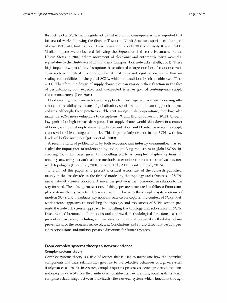
1. Generative models – the aim of these models is to generate a snapshot of a

topology. Among generative models, some are static (time independent

topologies) while some use growth (and other mechanisms). Furthermore, some

generative models include predefined global properties (such as degree

distribution, hierarchy and modularity) while others predefine a local property

(such as the attachment probability).

2. Evolving models – the aim of these models is to capture the microscopic

mechanisms underlying the temporal evolution of a network topology. These

models include growth and in some instances may include node deletion and link

rewiring. For a comprehensive summary of mechanisms underlying various evolving

network models, readers are referred to Albert and Barabasi (2002).

Figure 2 outlines the different perspectives offered by generative and evolving net-

work models.

Based on the above classification, both ER random and small-world network models are

static generative models as they imply a fixed number of nodes where links are placed be-

tween nodes using some random algorithm. These models are therefore less widely used

to model dynamical open systems, such as SCNs. However, the ER random model is gen-

erally used by researchers as a null model to test whether a real network property is statis-

tically significant or simply attributable to random connectivity (Kito et al., 2014).

It is noted that the result of any static generative model can also be obtained by an

evolving model (for example, an ER random network can be conveniently generated

using an evolving model with a specified growth process). In fact, any evolving model

Fig. 1 Comparison of random, small-world and scale free networks. Topological structure of benchmarknetwork models. Random and Small-world network topologies do not include hub nodes. In contrast,scale-free topologies are characterised by the presence of small number of highly connected hub nodesand a high number of feebly connected nodes. Presence of distinct hubs in scale-free networks makethem more vulnerable to targeted attacks, compared to random and small-world networks

Perera et al. Applied Network Science (2017) 2:33 Page 5 of 25

can be used for generative purposes. In this regard, the BA model, which is generally

considered as an evolving network model, can also be used for generative purposes, de-

pending on the study requirement.

An evolving network growth model governs the time evolution of networks by speci-

fying the way in which the new nodes connect with the existing nodes in the network

(Zhao et al., 2011a). This process is referred to as ‘attachment’ and various network

growth models comprise various ‘attachment rules’, which subsequently generate net-

works with distinct topologies as they evolve. For example, the mechanism underlying

generation of scale free networks has been successfully captured by the growth (in

terms of nodes) and preferential attachment mechanism presented in the BA model

(Barabási and Albert, 1999). Under preferential attachment, the probability pi that a

new node makes a connection to an existing node i with degree ki is given by:

pi ¼kiPj∈Nkj

where N is the set of nodes to which the new node could connect.

The BA model represents a ‘rich get richer’ process and the resulting scale-free net-

work topology can be used to model many real world networks, such as the World

Wide Web, power grids, metabolic networks and social networks (Surana et al., 2005).

This concept explains the existence of ‘hubs’ (a few nodes with a large number of con-

nections), which is a defining feature of scale-free networks.

The degree distribution Pk of a scale free network is approximated with power-law as

follows;

Pk∼k−γ

where k is the degree of the node and γ is the power-law exponent.

Many network properties depend on the value of the power-law exponent, γ

(Barabasi, 2014). Therefore, it is important to accurately estimate the power-law expo-

nent of the degree distribution of a given network topology, as this enables us to com-

pare network topologies on a continuous spectrum. Newman (2005) presents a reliable

Fig. 2 Modelling Perspectives obtained from Generative and Evolving Network Models

Perera et al. Applied Network Science (2017) 2:33 Page 6 of 25

methodology accurately estimating the power-law exponent of a given degree distribu-

tion, which involves plotting the complementary cumulative distribution function. This

method does not require data binning and as a result eliminates the plateau observed

in linear binning approach for high degree regime by extending the scaling region. In-

terested readers are referred to Clauset et al. (2009), for a comprehensive review of

power-law distributions in empirical data.

Fitness based network models

In the BA model, it is assumed that a node’s growth rate (in terms of new link acquisi-

tion) is determined solely by its degree. Accordingly, it predicts that the oldest node al-

ways has the most links – this concept is often referred to as the first mover advantage

in the economics literature. However, this approach does not take into consideration

the intrinsic characteristics of the nodes which may influence the rate at which they ac-

quire new links. For instance, in many real world networks such as Hollywood actor

networks and global business networks, some nodes despite being latecomers, acquire

links within a short timeframe whereas others are present within the network from

early on but fail to acquire high numbers of links (Barabasi, 2014). As such, modelling

SCN growth based on a growth model which views new link acquisitions from a purely

topological perspective may not be suitable.

Therefore, rather than relying entirely on the node degree, the attachment probability

and subsequent network growth should rely on a more basic factor, referred to as node

‘fitness’ (Caldarelli et al., 2002; Ghadge et al., 2010; Smolyarenko, 2014). The concept of

‘fitness’ can be thought of as the amalgamation of all the attributes of a given node that

contribute to its propensity to attract links, which could also include the node degree.

In order to overcome the limitations mentioned above, a model was proposed by

Bianconi and Barabasi (2001). This model is referred to as the Bianconi-Barabasi Model

(hereinafter referred to as the BB model) and has the following characteristics;

� Growth – At each time step, a new node j with m links and fitness ϕjis added to the

network. In generating an ensemble of networks, ϕj is sampled from a fitness

distribution. Once assigned, the fitness of a node remains constant.

� Preferential Attachment – the probability of a new node connecting to node i is

proportional to the product of node i’s degree ki and its fitness ϕi;

Pi ¼ kiϕiPj∈Nkjϕj

As can be seen from the above formulation, between two nodes i and j with the same

fitness (ϕi = ϕj), the one with the higher degree will have the higher probability of selec-

tion. Conversely, between two nodes i and j with the same degree (ki=kj) the node with

the higher fitness will be selected with a higher probability, thus indicating that even a

relatively new node, with only a few links, can acquire more new links rapidly, if it has

a higher level of fitness. As such, consideration is given to both fitness and the degree

of the nodes in the above growth model.

More recently, Ghadge et al. (2010) proposed a purely fitness based network growth

model, which accounts for the various factors that contribute to the likelihood of a new

Perera et al. Applied Network Science (2017) 2:33 Page 7 of 25

node being attracted to an existing node within a network. Such fitness based attach-

ment models can indeed be categorised as generative models. This type of models of-

fers greater flexibility owing to their ability to reproduce network topologies with fixed

global properties.

In the model proposed by Ghadge et al. (2010), the fitness ϕi, which represents the

propensity of node i to attract links, is formed from the product of relevant attributes

{φi1,…, φiL};

ϕi ¼Y

k∈Lφik

Where each attribute, φi is represented as a real non-negative value. Subsequently, it

is assumed that the number of attributes affecting a node’s attractiveness is sufficiently

large and are statistically independent. Therefore, by a version of the Central Limit

Theorem, the overall fitness ϕi will tend to be lognormally distributed, regardless of the

type of distribution of the individual factors (Nguyen and Tran, 2012). In a SCN con-

text, the attributes, which contribute to fitness, could include cost, service or product

quality, reliability, and so on. Finally, the probability of connecting a new node j to an

existing node i is taken to be proportional to its fitness ϕi, as follows;

pi ¼ϕiPj∈Nϕj

The above attachment rule, named the ‘Lognormal Fitness Attachment’ (LNFA),

differs from the BA model in that node fitness replaces node degree (Nguyen and

Tran, 2012). Therefore, in LNFA, a new node which has a large fitness, despite be-

ing in the network for a short period of time, can make itself a preferential choice

for new nodes entering the network.

Recent work by Bell et al. (2017) have investigated the evolutionary mechanisms that

would give rise to a fitness-based attachment process. In particular, it is proven by ana-

lytical and numerical methods that in homogeneous networks, the minimisation of

maximum exposure to unfitness by each node, leads to attachment probabilities that

are proportional to fitness. This result is then extended to heterogeneous networks,

with strictly tiered SCNs being used as examples.

Generating null models using configuration model

Similar to the LNFA model, the configuration model belongs to the wider class of net-

work generative models. A generative model allows us to choose parameters and draw

a single instance of a network. Since a single generative model can generate many in-

stances of networks, the model itself corresponds to an ensemble of networks.

The configuration model is commonly used to generate networks with pre-defined

degree sequences. It is particularly useful for generation of null models for the purposes

of hypothesis testing. Comparison of properties of an empirical network with the prop-

erties of an ensemble of networks generated by the configuration model allows one to

identify if the properties observed in the empirical network are unique and meaningful

or whether they are common to all networks with that degree sequence (Fosdick et al.,

2016). When data is available for an empirical network, a technique termed degree pre-

serving randomisation (DPR) is often used in literature to generate random networks

Perera et al. Applied Network Science (2017) 2:33 Page 8 of 25

which correspond to the configuration model. DPR involves rewiring the original net-

work, to generate an ensemble of null models, while preserving the degree vector

(Maslov and Sneppen, 2002). At each time step, the DRP process randomly picks two

connected node pairs and switch their link targets. This switching is repeatedly applied

to the entire network until each link is rewired at least once. The resulting network

represents a null model where each node still has the same degree, yet the paths

through the network have been randomised.

For example, Becker et al. (2014) have constructed a manufacturing system network

model from real world data (where nodes represent separate work stations and links

represent material flows between work stations). By applying the DPR process to gener-

ate an ensemble of networks with the same degree distribution, the authors observe

that nodes (work stations) with a particularly high betweenness centrality are over-

represented in the manufacturing system studied. They concludes that the manufactur-

ing system topology is therefore non-random and favours the existence of a few highly

connected work stations.

Network science approach to modelling the topology and robustness ofSCNsSo far, the published research in the area of modelling SCNs as complex networks

have demonstrated that a network perspective can indeed be used to successfully

represent a supply chain as nodes and links (Thadakamalla et al., 2004; Xuan et

al., 2011; Zhao et al., 2011a; Zhao et al., 2011b; Wen and Guo, 2012; Li et al.,

2013; Li, 2014; Mari et al., 2015 and Kim et al., 2015). A typical SCN model con-

sists of nodes, which represent individual firms (such as suppliers, manufacturers,

distributers and retailers), and links, which represent interactions between nodes

(such as exchange of information, transportation of material, and financial transac-

tions). Such abstractions can be beneficial in identifying the properties of various

types of SCN, as representing too many details could be detrimental to identifying

the network properties (Shen et al., 2006). On the other hand, important node or

link information could be lost. The level of detail to be represented by a given

complex network model is an important decision to be made by the network sci-

entist (Kasthurirathna, 2015).

Given the ultimate goal of obtaining generalizable results for real world SCNs, the

theoretical research in this area should be well informed by empirical studies. In par-

ticular, empirical studies should be used to establish the key characteristics that need to

be represented in the network topologies being generated by a given growth mechan-

ism. Figure 3 illustrates the general methodological framework of research on topo-

logical modelling and robustness analysis of SCNs.

Modelling SCN topologies through growth models

In order to characterise the dynamical processes on complex SCNs, the first step is to

construct realistic network growth models. Such models can be used to generate an en-

semble of networks with the required topological properties, from which insights can

be gained into the relationship between the topology and the dynamics of complex net-

works (Bianconi, 2016).

Perera et al. Applied Network Science (2017) 2:33 Page 9 of 25

In the context of supply chains, the concept of growth describes how newcomer

firms join existing firms in a SCN. As new entrants join the SCN, trading partners

are assigned from within the network. In the above regard, the BA model, despite

its simplicity and elegance, includes a number of known limitations, as listed in

Table 1 against their respective implications for SCNs.

Indeed, firm partner selection is, in reality, a multi-objective problem and involves

numerous factors, such as price, performance, quality, goodwill, transport cost (Jain et

al., 2009; Li et al., 2013). However, it is not practical to consider all these factors, so re-

searchers have adopted simple yet intuitive approaches which extend the basic BA

model concept. These include specifying selection (attachment) rules based on basic

topological properties, such as the node degree (i.e. the connectedness of a given firm),

in conjunction with other parameters (such as the number of links entering the system

with each type of new node, the rewiring probability, and the topological distance be-

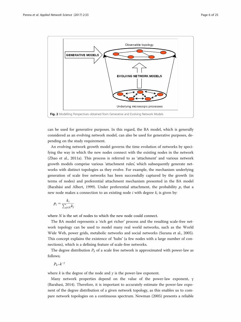
tween source and target nodes). Examples of such customised attachment rules are

summarised in Table 2.

Each of the aforementioned attachment rules, over time, generate networks with dis-

tinct topologies. It is evident, that when constructing network topologies representative

of SCNs, the attachment preference is generally governed by three factors;

1) The type of node entering the system (which determines the number of links that

enter the system with addition of new nodes and to which existing nodes these

links will be connected).

2) Type and degree of existing nodes (preference is given to existing high degree nodes

over the low degree nodes, representing the market power and visibility of highly

connected firms).

3) Type and topological or geographical distance of existing nodes (preference is given

to closer nodes than farther away ones, in terms of either the topological or the

Fig. 3 General methodological framework of research on topology and robustness of SCNs

Perera et al. Applied Network Science (2017) 2:33 Page 10 of 25

geographical distance, representing the ‘relationship distance’ or the cost of goods

movement, respectively).

Concept of SCN robustness

From the contemporary literature in the area of modelling SCN robustness, it is evident

that the terms resilience and robustness have been used interchangeably by researchers.

However, in the field of network science, the terms resilience and robustness have dis-

tinct meanings. For example, a system is called robust, if it can maintain its basic func-

tions in the presence of internal and external perturbations. Hence, a robust SCN

would include redundant or parallel components, which if needed can be relied upon

to maintain the overall functionality.

In contrast, resilience is defined as the capability of a system to adapt to internal or

external perturbations by changing mode of operation, without losing its ability to

function (Barabasi, 2014). Therefore, a resilient supply chain should respond quickly

and effectively to a given perturbation, such as a change in supply or demand, or to the

failure of a component (such as a firm or a material transport route) within the system.

The response mechanism of a resilient SCN is attributable to its flexibility to rewire the

lost connections away from disrupted nodes (Sheffi and Rice, 2005). As opposed to re-

silience, the robustness of a SCN does not relate to response mechanisms – it merely

reflects the extent to which a given SCN can withstand loss of its components, without

losing its basic functions. It is worth noting that most studies have focussed mainly on

the topological robustness of SCNs, rather than their resilience.

Table 1 Limitations of BA Model in Modelling SCNs

Limitation SCN modelling implication

Does not account for internal link formations(Barabasi, 2014)

In a SCN, new links may not only arrive with newfirms but can be created between the pre-existingfirms.

Cannot account for node deletion (Barabasi, 2014) Firms may exit a given SCN over time.

An isolated node is unable to acquire any linkssince according to preferential attachment, theprobability of a new node connecting to anisolated node is strictly zero (since the connectionprobability is governed by the existing number ofconnections).

In reality, any firm has a certain level of initialattractiveness.

Assumes that all firms within the supply networkare homogeneous in nature with no differentiationother than the topological aspects (Hearnshaw andWilson, 2013).

Real SCNs include firms with high levels ofheterogeneity beyond the number of dealings orconnections with other firms.

The key requirement of the preferential attachmentrule is that every new node joining the networkmust possess complete and up-to-date informationabout the degrees of every existing node in thenetwork.

Such information is unlikely to be readilyavailable in a real world setting – for example,when considering a manufacturer for a newpartnership, full information about the number oftheir current suppliers and clients is unlikely tobe available (Smolyarenko, 2014). Therefore, analgorithm which relies on local information isdeemed more suitable. For example, see Vázquez(2003).

Network growth by preferential attachment producesa decaying clustering coefficient as the networkexpands.

May not be a realistic representation of exchangerelationships and concentration of power in firmswithin the real SCNs (Hearnshaw and Wilson,2013).

Perera et al. Applied Network Science (2017) 2:33 Page 11 of 25

Analytical measurements of SCN topological robustness

Network science offers a rich set of tools for topological robustness analysis. Refer to

Costa et al. (2007) and Rubinov and Sporns (2010) for a comprehensive range of mea-

sures used for the characterization of complex networks. Some key metrics used in net-

work science, and their corresponding SCN implications at node and network level are

presented in Appendix 1 and 2, respectively.

As can be seen from the metrics presented in Appendix 1 and 2, the analytical

measures in network science can be used to gain important insights on network

structure and robustness quickly and with low computational difficulty. However,

the key limitation of using analytical measures is that they are unable to account

Table 2 Key features of customised attachment rules used in literature

Customised attachment Rule Key features

Ad hoc attachment rules based on the militarysupply chain example, used by Thadakamalla et al.(2004)

Three types of nodes can enter the system in apre-specified ratio. Each type of node has a specificnumber of links. Attachment rule depends on thetype of node entering the system. The first link of anew node entering the system attaches to an exist-ing node preferentially, based on the degree. Thesubsequent links, entering the system with eachnew node, attach randomly to a node at a pre-specified topological distance (also referred to asthe ‘hop count’, which denotes the least number oflinks required to be traversed in order to reach agiven node from another).

Degree and Locality based Attachment (DLA), used byZhao et al. (2011a).

A node entering the system considers both thedegree and the distance of an existing node, whenestablishing connections. In particular, attachmentpreference for the first link arriving with each newnode is calculated preferentially based on thedegree of the existing nodes. If the node is allowedto initiate more than one link, the subsequent linkswill attach preferentially to existing nodes based ontopological distance. Tunable parameters are usedto control the responsiveness of attachmentpreference to both the degree and the topologicaldistance.

Randomised Local Rewiring (RLR), used by Zhao et al.(2011b)

This model is applied to an existing network, byiterating through all links and considering thenodes at either end of each link. With apredetermined rewiring probability, to control theextent of rewiring, each link will disconnect fromthe highest degree node it is currently connectedwith and reconnect with a randomly chosen nodewithin a pre-specified maximum radius (which caneither be geographical or topological).

Evolving model used by Zhang et al. (2012) and Liand Du (2016)

Start with a random network that consists of a pre-specified number of supply nodes with randomlyassigned (x, y) coordinates. Supply and demandnodes are sequentially added to the system, accord-ing to a pre-specified supply-demand ratio. If thenew node is a supply node, the first link will con-nect to an existing supply node in the system whileother links are connected randomly to existingnodes. If the new node is a demand node, all linkswill connect with existing supply nodes in the sys-tem, with connection probability based on theproduct of degree and the geographical distance.Similar to DLA discussed above, tunable parametersare used to control the responsiveness of attach-ment preference to both the degree and the geo-graphical distance.

Perera et al. Applied Network Science (2017) 2:33 Page 12 of 25

for the heterogeneity of nodes, in terms of their functionality within a given SCN,

since the metrics consider all nodes to be homogeneous in function. In order to

overcome the above limitation, researchers have relied on simulations to analyse

the topological robustness of SCNs. Furthermore, simulations allow flexibility in

analysis through customised robustness metrics (see section below).

Using simulations to determine the topological robustness of SCNs

Node failures in networks can be categorised either as ‘random failures’ or ‘tar-

geted attacks’. Random failures entail the same probability of failure across each

node within a given network. In contrast, a ‘targeted attack’ refers to when an at-

tacker selectively compromises the nodes with probabilities proportional to their

degrees, where highly connected nodes are compromised with higher probability

(Ruj and Pal, 2014).

In the network science literature, random failures and targeted attacks in networks

are typically simulated as follows;

1) Random failure: Each robustness metric established for the network is recorded at

each time step by randomly removing the nodes from the network.

2) Targeted attacks: Each robustness metric established for the network is recorded at

each time step by sequentially removing the nodes, based on their degree, removing

higher degree nodes first, from the network.

The robustness values recorded for each metric, for each network considered, are

then compared. It has, so far, been established that the random networks respond simi-

larly to both random failures and targeted attacks. In comparison, the scale-free net-

works are robust against random failures but are highly sensitive to targeted attacks

(Albert et al., 2000). This is due to the presence of hubs (highly connected nodes) in

scale-free networks, which are the nodes targeted by an attacker.

A number of researchers have modelled various SCN topologies under both ran-

dom failures and targeted attacks, and attempted to establish an optimal topology

which can withstand each type of failure without compromising the overall net-

work functionality (Thadakamalla et al., 2004; Zhao et al., 2011a, Li and Du, 2016).

Each study has established a set of robustness metrics, in order to assess and com-

pare the robustness of each network topology simulated under random failures and

targeted attacks. These robustness metrics are variations of the existing standard

topological metrics from network science. The most commonly used network top-

ology metrics in supply network research are;

1. Size of the largest connected component (LCC) of a network - As nodes are

sequentially removed, the graph disintegrates into sub-graphs. The number of nodes

in the LCC (or the largest sub-graph) of a fragmented network therefore provides

insights into its overall connectivity.

2. Average or maximum path length in the LCC - The average or maximum shortest

path length between any two nodes in the largest connected component of a

network. This provides insights into the overall accessibility of the network.

Perera et al. Applied Network Science (2017) 2:33 Page 13 of 25

The above metrics consider the roles of entities (nodes and links) within a distri-

bution network to be homogeneous. Such an assumption is far from reality, since

the entities within a real-world supply network play different roles with different

characteristics – for example, the distance between two supply nodes or two de-

mand nodes are not as important as that between a supply and a demand node

(Zhao et al., 2011b).

Therefore, various researchers (such as Thadakamalla et al., 2004; Zhao et al.,

2011a and Zhao et al., 2011b, Xu et al., 2014) have developed new metrics, which

realistically represent the heterogeneous roles of nodes within the network. For ex-

ample, Zhao et al. (2011a) have developed the following customised robustness

metrics for distribution networks;

� Supply availability rate is represented as the percentage of demand nodes that have

access to supplies from at least one supply node.

� The network connectivity is determined through the size of the largest functional

sub-network (LFSN), namely the number of nodes in the LFSN in which there is a

path between any pair of nodes and there exists at least one supply node.

� Accessibility is determined by;

� ○ Average supply path lengths in the LFSN, i.e. the average shortest supply path

length between all pairs of supply and demand nodes in the LFSN.

� ○ Maximum supply path lengths in the LFSN, i.e. the maximum shortest path

length between any pair of supply and demand nodes in the LFSN.

Empirical studies on SCN topologies

A review of contemporary literature on SCN topologies reveals that only a limited

number of data driven studies are available in this domain. This is mainly due to diffi-

culty in obtaining specific information about supplier/customer relationships, which is

often proprietary and confidential. Table 3 presents a summary of a number of empir-

ical studies available to date. It is noted that these studies generally focus on overall

topological character of SCNs rather than robustness.

Discussion of literature – Limitations and improved methodologicaldirectionsThis section will critically discuss the existing methodologies in contemporary litera-

ture, on modelling SCN topologies and robustness.

Modelling SCN topologies

Insights revealed by empirical studies

While SCNs in real world may not evolve through a single mechanism, it is possible to

infer general growth and design principles from the global properties of existing SCNs.

In this regard, empirical studies play a major role in pointing the theoretical research

work on modelling SCN topologies in a meaningful direction.

A number of past theoretical studies have relied upon the BA model for SCN

growth and/or benchmarking purposes (Thadakamalla et al., 2004; Xuan et al.,

2011; Zhao et al., 2011a). However, based on the results of empirical studies

Perera et al. Applied Network Science (2017) 2:33 Page 14 of 25

Table 3 Summary of empirical studies of SCN topologies

Study Data source and SCNs considered Key findings

Parhi (2008) Customer-supplier linkage network in theIndian auto component industry has beenconsidered (618 firms), using the data fromthe Auto Component ManufacturersAssociation of India.

The Indian auto component industry SCN wasfound to be scale free in topology, with apower-law exponent, γ = 2.52a.

Keqiang et al. (2008) Guangzhou automotive industry supply chainnetwork has been investigated. Data has beencollected from 94 manufacturers, betweenNovember 2007 and January 2008.

Guangzhou automotive industry SCN wasfound to be scale-free in topology. Based onthe data presented by the authors, we havecalculated the power-law exponent of the de-gree distribution, γ to be 2.02.

Kim et al. (2011) Three case studies of automotive supplynetworks (namely, Honda Accord, Acura CL/TL,and Daimler Chrysler Grand Cherokee)presented by Choi and Hong (2002).

This study has developed SCN constructsbased on a number of key network and nodelevel analysis metrics. In particular, the rolesplayed by central firms, as identified by variousnetwork centrality measures, have beenoutlined in the context of SCNs.

Büttner et al. (2013) Present network analysis results for a porksupply chain of a producer community inNorthern Germany. Data has been obtainedby the producer community for a period of3 years.

Reports that the degree distribution of theSCN follows power law (in and out degreedistributions follow power-law with power-lawexponents, γ = 1.50 and γ = 1.00, respectively).Disassortative mixingb has been observed interms of node degree.

Kito et al. (2014) A SCN for Toyota has been constructed usingthe data available within an online databaseoperated by Marklines AutomotiveInformation Platform.

The authors have identified the tier structure ofToyota to be barrel-shaped, in contrast to thepreviously hypothesized pyramidal structure.Another fundamental observation reported inthis study is that Toyota SCN topology wasfound to be not scale free.

Brintrup et al. (2015) Airbus SCN data obtained from Bloombergdatabase.

Reports that the Airbus SCN illustrates power-law degree distribution, i.e. scale free top-ology, with a power-law exponent, γ = 2.25a.Assortative mixing was observed based onnode degree and community structures werefound based on geographic locations of thefirms.

Gang et al. (2015) Authors have investigated the urban SCN ofagricultural products in mainland China. Datacollection is based on author observationsover 2 years.

The SCN of agricultural products was found tobe scale free in topology, with a power-lawexponent, γ = 2.75. High levels of disassorta-tive mixingb has been observed in terms ofnode degree.

Orenstein (2016) SCN data for food (General Mills, Kellogg’sand Mondelez) and retail (Nike, Lowes andHome Depot) industries have been obtainedfrom Bloomberg database.

The SCNs considered in this study were found tohave scale free topologies with γ < 2. Inparticular, for the food industry SCNs for GeneralMills, Kellogg’s and Mondelez were found to haveγ = 1.25, 1.47 and 1.56, respectively. For the retailindustry, the SCNs for Nike, Lowes and HomeDepot were found to have γ = 1.83, 1.73 and1.67, respectively.

Perera et al. (2016b) Analysis has been undertaken for 26 SCNs(which include more than 100 firms) out of38 multi echelon SCNs presented in Willems(2008) for various manufacturing sectorindustries.

22 out of the 26 SCNs analysed display 80% orhigher correlation with a power-law fit, withpower-law exponent γ = 2.4 (on average). Fur-thermore, these SCNs were found to be highlymodularb and robust against random failures.Also, disassortative mixingb was observed onthese SCNs.

Sun et al. (2017) A GIS based SCN structure has been simulatedfor the automobile industry using the data of toptwelve car brands of Chinese market in recentfive years as basic parameters.

The Chinese automobile SCN simulated usingreal world data as basic parameters, indicatesthat the degree distribution conforms to thepower-law, with a power-law exponent,γ = 3.32.

aNote that in some research papers, the power-law exponent is presented for the cumulative degree distribution.In such cases, the power-law exponent of the degree distribution has been established by adding 1 tothe power-law exponent of the cumulative degree distribution since the power-law exponent of thecumulative degree distribution is 1 less than the power-law exponent of the degree distribution(Newman, 2005). These instances have been identified with an asterisk in Table 2bRefer to Appendix 1 for detailed definitions (including mathematical formulations) of these metrics

Perera et al. Applied Network Science (2017) 2:33 Page 15 of 25

summarised in this paper, it is understood that the BA model (due to its minimal

nature) cannot sufficiently represent the growth mechanism underlying SCNs, due

to the following:

1) The BA model generates networks with a constant power-law exponent, γ = 3, as

shown by both analytical and simulation methods in Barabasi (2014). The SCNs re-

ported in empirical studies indicate topologies with γ ≈ 2 (it is noted that γ = 2 is

the boundary between hub and spoke (γ < 2) and scale-free (γ > 2) network

topologies).

2) The BA model cannot generate networks with pronounced community structure,

which has been observed in real SCNs, since all nodes in the network belong to a

single weakly connected component (Newman, 2003).

3) Assortative (or disassortative) mixing as observed in real SCNs, is not a feature of

networks generated by the BA model - as shown analytically (in the limit of large

network size) by Newman (2002).

As can be seen above, although some real world networks have been convin-

cingly modelled by the preferential attachment mechanism presented in the BA

model (Barabasi et al., 1999, Albert et al., 1999), this is not so for SCNs. Therefore,

a convincing network growth mechanism for SCNs is yet to be formulated.

Suitability of network models in literature for SCN modelling purposes

Considering the limitations of the BA model in representing the topologies of real

SCNs (as discussed in the previous section), the generative models which predefine

a global property (such as the degree distribution, hierarchy, modularity, etc.) are a

good starting point for the researchers in the SCN domain, especially when the

interest of research is directed towards understanding the role of network topology

on its robustness. In particular, the SCNs in the real world may have evolved based

on various non generalizable principles. Therefore, when aiming to study and

understand the topological character of SCNs, researchers will benefit more from

simply mimicking the observed topologies, than trying to understand the under-

lying growth mechanism – which may indeed be complex and non-generalizable,

beyond the realm of a single mathematical algorithm.

Generative models allow the researchers to recreate a network topology, as ob-

served at a single cross section in time, and undertake further investigations on

various phenomena, such as topological efficiency, robustness etc. When informa-

tion on the adjacency matrix is available for real-world networks, one can simply

use the DPR to generate an ensemble of random networks (which correspond to

the configuration model) to establish whether the degree distribution on its own is

sufficient to describe the property observed in the network at hand. It is worth

noting that in tiered SCNs, the DPR process should be restricted to each tier, in

order to ensure that links are not swapped between non-compatible tiers.

In many cases, adjacency matrix information for real networks are not readily available.

Such situations require the researcher to recreate the degree distribution of the SCN,

using only the basic network metrics (such as the power-law exponent) or simply through

qualitative descriptions. In this regard, fitness based generative models have recently

Perera et al. Applied Network Science (2017) 2:33 Page 16 of 25

gained prominence in theoretical research (Caldarelli et al., 2002; Bedogne et al., 2006;

Smolyarenko, 2014; Perera et al., 2016a). In fitness based models, the fitness distribution

and the connection rules are given by a priori arbitrary functions, which enables consider-

able amount of tuning (Smolyarenko, 2014). Indeed, this tunability makes such models a

useful and practical modelling tool.

For example, the LNFA includes a tunable parameter σ (the shape parameter of

the lognormal distribution), which can be manipulated to generate a large

spectrum of networks. At one extreme, when σ is zero, all nodes have the same

fitness and therefore at the time a new node joins the network, it chooses any

existing node as a neighbour with equal probability, thus replicating the random

graph model. On the other hand, when σ is increased beyond a certain threshold,

very few nodes will have very large levels of fitness while the overwhelming major-

ity of nodes have extremely low levels of fitness. As a result, the majority of new

connections will be made to a few nodes which have high levels of fitness. The

resulting network therefore resembles a monopolistic/“winner-take-all” scenario,

which can sometimes be observed in the real world (however, in some instances, it

may be necessary to place a restriction on the highest degree achievable by a single

node, in order to represent the ‘contractual capacity’ of firms). Between the above

two extremes (random and monopolistic) lies a spectrum of power law networks

which can closely represent many real networks (Ghadge et al., 2010). Figure 4 il-

lustrates the spectrum of network topologies generated by the LNFA model.

Nguyen and Tran (2012) have illustrated that the LNFA model can indeed generate

network topologies with γ ≈ 2, which represents many observed SCN topologies in em-

pirical research work (Büttner et al., 2013; Orenstein, 2016). However, the ability of

LNFA to generate modular and disassortative networks, as observed in SCNs, remains

an open research question.

Directionality of links

The inter-firm relationships in SCNs are generally modelled using undirected links.

However, the links between nodes in a SCN can include a direction, depending on the

specific type of relationship being modelled. The inter-firm relationships in a SCN

can be broadly categorised into three classes, namely; (1) material flows, (2) financial

flows, and (3) information exchanges. Material flows are usually unidirectional from

suppliers to retailers, while financial flows are unidirectional in the opposite direction.

Both material and financial flows mostly occur vertically, across the functional tiers of

a SCN (however, in some cases, two firms within the same tier, such as two suppliers,

Fig. 4 Transitions from random to winner-take-all graphs observed as σ parameter is increased

Perera et al. Applied Network Science (2017) 2:33 Page 17 of 25

could also exchange material and finances) (Lazzarini et al., 2001). In contrast, infor-

mation exchanges are bidirectional (i.e. undirected) and includes both vertical and

horizontal connections (i.e. between firms across tiers and between firms within the

same tier). Therefore, the same SCN can include different topologies based on the

specific type of relationship denoted by the links in the model. For instance, unlike

material and financial flows, SCN topology for information exchanges can exhibit

shorter path lengths and high clustering due to relatively larger number of horizontal

connections (Hearnshaw and Wilson, 2013).

Compared to undirected network representation, in directed networks, the adja-

cency matrix is no longer symmetric. As a result, the degree of a node in a di-

rected network is characterised by both in-degree and out-degree. On this basis,

the degree distribution of directed networks is analysed separately for in and out

degrees. Also, unlike undirected networks, in directed networks the distance be-

tween node i and node j is not necessarily the same as the distance between

node j and node i. In fact, in directed networks, the presence of a path from

node i to node j does not necessarily imply the presence of a path from node j

to node i (Barabasi, 2014). This has implications on node centrality metrics, such

as closeness and betweenness. In addition, it is noted that many dynamics, such

as synchronizability and percolation, are different in directed networks compared

to undirected networks (Schwartz et al., 2002; Park and Kim, 2006). Therefore,

when modelling SCNs, it is important to first identify the specific type of rela-

tionship denoted by the links, so that network can be correctly represented as

undirected or directed.

Additional considerations for robustness testing

From a SCN point of view, the position of an individual firm with respect to the

others can influence both its strategy and behaviour (Borgatti and Li, 2009). Ac-

cordingly, analysis of each firm’s role and importance based on its position in the

SCN can reveal important properties, such as its structural robustness. In this re-

gard, future studies could simulate targeted attacks based on node centrality mea-

sures, such as betweenness and closeness centrality, rather than node degree. Such

considerations will capture the critical nodes in various perspectives. Also, as

Piraveenan et al. (2012) notes, when simulating targeted attacks on empirical net-

works, one could also rank nodes on the basis of non-topological attributes (such

as firm size, output, and geographic location).

Depending on the structure of the overall SCN, disruptions can be experienced

in various forms, such as; supply disruptions, logistics disruptions, coordination

disruptions and demand disruptions (Yi et al., 2013). These various disruptions

can be attributed to either nodes or links or both, for modelling purposes. So far,

the focus of modelling has been on unweighted links in SCNs, which essentially

indicate that all relationships are considered to be homogeneous in terms of their

relative importance. However, real SCNs exhibit large levels of heterogeneity in

the capacity and intensity of the connections (links) between the nodes. Rui and

Ban (2012) state that empirical observations have shown the existence of nontriv-

ial correlations and associations between link weights and topological quantities

Perera et al. Applied Network Science (2017) 2:33 Page 18 of 25

in complex networks. In the context of SCNs, the connections, be they physical

flows or relationships between organisations, are heterogeneous in terms of the

strength and importance. Therefore, the SCN can be better reflected and under-

stood in terms of weighted networks, where weights reflect volume, frequency or

the criticality of flows (Hearnshaw and Wilson, 2013). If such information is

available, targeted attacks could also be simulated by link removal on the basis of

link weights.

Conclusions and future directionsThis paper has presented a comprehensive and critical review of the research

undertaken on the use of network science techniques to model the topology and

robustness of SCNs. The key challenge in this research is the tailoring of network

science principles to SCNs, by identifying the fundamental SCN features. Although

network science offers a rich conceptual representation of SCNs, a number of po-

tential improvements to the existing modelling approach have been identified and

are proposed for future research.

From the literature reviewed, it is evident that most of the previous research

undertaken in the field of modelling SCNs as complex networks have given pri-

mary consideration to network topology. Based on the empirical studies, it is evi-

dent that most real world SCNs tend to have power-law exponents which fluctuate

around 2. It is noted that γ = 2 is the boundary between hub and spoke (γ < 2)

and scale-free (γ > 2) network topologies. Also, most SCN topologies indicate dis-

assortative mixing and modularity (the presence of communities). The well-known

BA model is not able to generate network topologies with the above mentioned

features. Therefore, researchers are advised to focus on generative models to mimic

the SCN topologies observed in empirical studies. This approach is deemed more

effective and reliable than the existing methodology of investigating the mecha-

nisms underlying SCN evolution, particularly since the overarching goal of research

in this area is to understand the role of network topology on properties such as

robustness. It is emphasised that future theoretical work on development of SCN

growth models should ideally aim to reflect the above outlined topological features

in the network topologies obtained from generative models. A natural extension of

this work would be to investigate the ability of fitness based growth models,

coupled with node and link heterogeneity, to mimic the topological features, such

as modularity and disassortativity, of real world SCNs.

So far, empirical studies have investigated a cross sectional view of real SCNs

at a given point in time. However, databases such as Bloomberg offer rich data

sets to investigate the evolution of SCNs across time. Therefore, researchers

could investigate the evolution of SCNs, using temporal data. Such empirical tests

can validate the theoretical network growth models developed so far in the

literature.

Appendix 1LIST OF NETWORK LEVEL METRICS AND THEIR SCN IMPLICATIONS.

Perera et al. Applied Network Science (2017) 2:33 Page 19 of 25

Table 4 Network level metrics and their SCN implications

Mathematical representation SCN implication

Average degree (<k>)

< k >¼P

iki

Nwhere N is the total number of nodes in the network

Indicates, on average, how many connections a givenfirm has. Higher average degree implies good inter-connectivity among the firms in the SCN, which isfavourable in terms of efficient exchange of informa-tion and material.In directed networks, the in-degree characterises thenumber of supply channels while the out-degree indi-cates the number of sales channels, of a given firm.

Network diameter

diameter ¼ maxi;j l i; jð Þwhere l is the number of hops traversed along theshortest path from node i to j.

The diameter of a SCN is the largest distance betweenany two firms in the network, in terms of number ofintervening links on the shortest path. More complexmanufacturing processes can include large networkdiameters (i.e. many stages of production) indicatingdifficulty in governing the overall SCN under acentralised authority.

Network density (D)

D ¼ <k>N−1

where <k > is the mean degree of all the nodes andN is the total number of nodes, in the network

Density of a SCN indicates the level ofinterconnectivity between the firms involved. SCNswith high density indicate good levels of connectivitybetween firms which can be favourable in terms ofefficient information exchange and improvedrobustness due to redundancy and flexibility (Sheffiand Rice, 2005).

Network centralisation (C)

C ¼ NN−2

max kð ÞN−1 −D

� �

where N is the total number of nodes in the networkand max(k) is the maximum degree of a node withinthe network. Density is determined as per theequation above.

Network centralisation provides a value for a givenSCN between 0 (if all firms in the SCN have the sameconnectivity) and 1 (if the SCN has a star topology).This indicates how the operational authority isconcentrated in a few central firms within the SCN.Highly centralised SCNs can have convenience interms of centralised decision implementation and highlevel of controllability in production planning.However, highly centralised SCNs lack localresponsiveness since relationships between firms invarious tiers are decoupled (Kim et al., 2011).

Network heterogeneity (H)

H ¼ffiffiffiffiffiffiffiffiffiffiffiffiffiffiffivariance kð Þ

p<k>

where <k > is the mean degree and variance (k) is thevariance of the degree, of all the nodes in thenetwork.

Heterogeneity is the coefficient of variation of theconnectivity. Highly heterogeneous SCNs exhibit hubfirms (i.e. firms with high number of contractualconnections). In extreme cases, there may be manysuper large hubs (winner take all scenario, indicatingcentralised control of the overall SCN through a singlefirm or a very few firms).

Average clustering coefficient (<C>)

< C >¼P

iCi

N

where N is the total number of nodes in the networkand Ci is the number of triangles connected to node idivided by the number of triples centered aroundnode i.

Clustering coefficient indicates the degree to whichfirms in a SCN tend to cluster together around a givenfirm. For example, it can indicate how various suppliersbehave with respect to the final assembler at theglobal level (Kim et al., 2011). Therefore, the higher theclustering coefficient, the more dependent suppliersare on each other for production (Brintrup et al., 2016).

Power-law exponent (γ) (Barabasi and Albert, 1999)

The degree distribution Pk of a scale free network isapproximated with power law as follows;Pk ∼ k

−γ

where k is the degree of the node and γ is the power-law exponent (also known as the degree or scale freeexponent).

SCNs with γ < 2 include very large hubs which acquirecontrol through contractual relationships with otherfirms at a rate faster than the growth of the SCN interms of new firm additions. As γ continues to increasebeyond 2, the SCNs include smaller and less numeroushubs, which ultimately leads to a topology similar to

Perera et al. Applied Network Science (2017) 2:33 Page 20 of 25

Appendix 2LIST OF NODE LEVEL METRICS AND THEIR SCN IMPLICATIONS.

Table 4 Network level metrics and their SCN implications (Continued)

that of a random network where all firms have almostthe same number of connections.Note that in directed networks, two γ values aregenerally reported – one for the in-degree and an-other for the out-degree.

Assortativity (ρ) (Newman, 2002)

Assortativity is defined as a correlation function ofexcess degree distributions and link distribution of anetwork.For undirected networks, when degree distribution isdenoted as pk and excess degree (remaining degree)distribution is denoted as qk, one can introduce thequantity ej,k as the joint probability distribution of theremaining degree distribution of the remainingdegrees of the two nodes at either end of a randomlychosen link.Given these distributions, the assortativity of anundirected network is defined as;

ρ ¼ 1σ2q

Pjk jk ej;k−qjqk

� �h i

where σq is the standard deviation of qk.

Positive assortativity means that the firms with similarconnectivity would have a higher tendency to connectwith each other (for example, highly connected firmscould be managing sub-communities in certain areasof production and then connect to other high-degreefirms undertaking the same function). This structurecan lead to cascading disruptions – where a disruptionat one leaf node can spread quickly within the net-work through the connected hubs (Brintrup et al.,2016).In contrast, a negative assortativity (i.e. disassortativity)indicates that it is the firms with dissimilar connectivitythat tend to pair up in the given network. Anunfavourable implication of disassortativity in SCNs isthat since high degree firms are less connected to oneanother, many paths between nodes in the networkare dependent on high degree nodes. Therefore,failure of a high degree node in a disassortativenetwork would have a relatively large impact on theoverall connectedness of the network (Noldus andVan, 2015).On the other hand, disassortative networks aregenerally resilient against cascading impacts arisingfrom targeted attacks – since hub nodes are notconnected with each other, the likelihood ofdisruption impacts cascading from one hub node toanother is minimised (Song et al., 2006).

Modularity (Q) (Newman and Girvan, 2004)

Q ¼ Pks¼1

lsL −

ds2L

� �2h i

where k is the number of modules, L is the number oflinks in the network, ls is the number of links betweennodes in module s, and ds is the sum of degrees ofnodes in the module s.To avoid getting a single module in all cases, thismeasure imposes Q = 0 if all nodes are in the samemodule or nodes are placed randomly into modules.

SCNs with high modularity contain pronouncedcommunities – i.e. partially segregated subsystems ormodules embedded within the overall SCN system(Ravasz et al., 2002; Newman, 2003). Each of thesesubsystems are generally responsible for a particularspecialised task.

Percolation threshold for random node removal (fc) (Cohen et al., 2000)

The percolation threshold for random node removal isgiven as;f c ¼ 1− 1

<k2><k> −1

where <k > is the mean degree and <k2 > is thesecond moment of the degree, of all the nodes in thenetwork.

The percolation threshold of a SCN indicates thepercentage of firms needed to be randomly removedprior to the overall SCN breaks into manydisconnected components (when the giantcomponent ceases to include all the nodes). Insummary, this indicates the number of random firmfailures that would drive the SCN from a connectedstate to a fragmented state (loss of overallinterconnectivity).

Perera et al. Applied Network Science (2017) 2:33 Page 21 of 25

Table 5 Node level metrics and their SCN implications

Mathematical representation SCN Implication

Degree (k)

The degree ki of any node i is represented by;ki ¼

Pj aij

where aij is any element of the adjacency matrix A.

Represents the number of direct neighbours(connections) a given firm has. For instance, in agiven SCN, the firm with the highest degree (suchas the integrators that assemble components) isdeemed to have the largest impact on operationaldecisions and strategic behaviours of other firms inthat particular SCN. Such a firm has the power toreconcile the differences between various otherfirms in the SCN and align their efforts with greaterSCN goals (Kim et al., 2011).In directed networks, the firms which have high in-degree are considered to be ‘integrators’ who collectsinformation from various other firms to create highvalue products. In contrast, the firms which have highout-degree are considered to be ‘allocators’ who aregenerally responsible for distribution of σs , t(n)high de-mand resources to other firms and/or customers.

Betweenness centrality (normalised) (Freeman, 1977)

The betweenness centrality of a node n is defined as;Cb nð Þ¼ 2

N−1ð Þ N−2ð ÞP

s≠n≠tσs;t nð Þ

σs;twhere s and t are nodes in the network, which aredifferent from n, σs , tdenotes the number of shortestpaths from s to t, and is the number of shortest pathsfrom s to t that n lies on.

Betweenness centrality of a firm is the number ofshortest path relationships going through it,considering the shortest path relationships thatconnect any two given firms in the SCN. Therefore, itindicates the extent to which a firm can intervene overinteractions among other firms in the SCN by being agatekeeper for relationships. Those firms with highlevels of betweenness generally play a vital role inSCNs – mainly owing to their ability to increase theoverall efficiency of the SCN by smoothing variousexchange processes between firms.

Closeness centrality (Sabidussi, 1966)

The closeness centrality of a node n is defined as;

Cc nð Þ ¼ 1<L n;mð Þ>

where <L(n,m) > is the length of the shortest pathbetween two nodes n and m (note that forunweighted graphs with no geodesic distanceinformation, each link is assumed to be one unit ofdistance). The closeness centrality of each node is anumber between 0 and 1.

Closeness centrality is a measure of the time that ittakes to spread the information from a particular firmto the other firms in the network. While it is closelyrelated to betweenness centrality, closeness morerelevant in situations where a firm acts as a generatorof information (i.e. a navigator) rather than a meremediator/gatekeeper.For example, due to various hindrances, the marketdemand information can easily be distorted when itflows from the downstream firms towards upstreamfirms. Such distortions can lead to undue deviationbetween production plans of manufacturers andsupply plans of suppliers, leading to a phenomenonknown as the bullwhip effect in supply chains. Firmswith high closeness centrality levels therefore play amajor role in sharing the actual market demandinformation with upstream firms in the SCN, thusdiminishing the adverse impacts arising frombullwhip effect (Xu et al., 2016).

Eigenvector centrality (Ruhnau, 2000)

If the centrality scores of nodes are given by the matrixX and the adjacency matrix of the network is A, theneach row of matrix X, namely x, can be defined as;

x∝Ax

i:e:

λx ¼ Ax

The eigenvector centrality scores are obtained bysolving this matrix equation. It can be shown that,while there can be many values forλ, only the largestvalue will result in positive scores for all nodes, so thisis the eigenvector chosen.

Eigenvector centrality measures a firm’s influence in theSCN by taking into account the influence of itsneighbours. The centrality scores are given by theeigenvector associated with the largest eigenvalue. Itassumes that the centrality score of a firm isproportional to the sum of the centrality scores of theneighbours. A firm with a high eigenvector centrality isassumed to derive its influential power through itshighly connected neighbours.

Perera et al. Applied Network Science (2017) 2:33 Page 22 of 25

FundingThe authors would like to acknowledge the Australian Research Council (ARC) for funding this work under grantDP140103643.

Availability of data and materialsNot applicable.

Authors’ contributionsSP carried out the initial review of literature and prepared the draft manuscript. M.G.H. Bell and M.C.J. Bliemerparticipated in discussions where limitations in existing research methods were identified and improvementsproposed. SP and M.G.H. Bell prepared the final manuscript. All authors read and approved the final manuscript.

Ethics approval and consent to participateNot applicable.

Consent for publicationNot applicable.

Publisher’s NoteSpringer Nature remains neutral with regard to jurisdictional claims in published maps and institutional affiliations.

Received: 1 June 2017 Accepted: 29 August 2017

ReferencesAlbert R, Barabási AL (2002) Statistical mechanics of complex networks. Rev Mod Phys 74(1):47Albert R, Jeong H, Barabási AL (1999) Internet: diameter of the world-wide web. Nature 401(6749):130–131Albert R, Jeong H, Barabási AL (2000) Error and attack tolerance of complex networks. Nature 406:378–382Barabási, A. L. (2014). Network science book. Boston: Center for Complex Network, Northeastern University. Available

online at: http://barabasi.com/networksciencebookBarabási A-L, Albert R (1999) Emergence of scaling in random networks. Science 286(5439):509–512Bartos S (2012) Resilience in the Australian food supply chain. Department of agriculture Australian government,

fisheries and forestry, Commonwealth of Australia, Canberra Retrieved from http://www.tisn.gov.au/Documents/Resilience%20in%20the%20Australian%20food%20supply%20chain%20-%20PDF%20copy%20for%20web.PDF

Bar-Yam Y (2002) General features of complex systems. Encyclopedia of Life Support Systems (EOLSS), UNESCO, EOLSSPublishers, Oxford

Becker T, Meyer M, Windt K (2014) A manufacturing systems network model for the evaluation of complexmanufacturing systems. Int J Product Perform Manag 63(3):324–340

Bedogne C, Rodgers GJ (2006) Complex growing networks with intrinsic vertex fitness. Phys Rev E 74(4):046115Bell M, Perera S, Piraveenan M, Bliemer M, Latty T, Reid C (2017) Network growth models: a behavioural basis for

attachment proportional to fitness. Sci Rep 2017:7Berryman MJ, Angus SD (2010) Tutorials on agent-based modelling with NetLogo and network analysis with Pajek,

Complex physical, biophysical and Econophysical systems, pp 351–375Bianconi G, Barabási AL (2001) Competition and multiscaling in evolving networks. EPL (Europhysics Letters) 54(4):436Bianconi, Ginestra. "Processes on networks". 2016. LectureBondy JA, Murty USR (1976) Graph theory with applications, vol 290. Macmillan, LondonBorgatti SP, Li X (2009) On social network analysis in a supply chain context*. J Supply Chain Manag 45(2):5–22Brintrup, A., Wang, Y., & Tiwari, A. (2015). Supply networks as complex systems: a network-science-based

characterizationBrintrup A, Ledwoch A, Barros J (2016) Topological robustness of the global automotive industry. Logist Res 9(1):1–17Buckley W (2008) Society as a complex adaptive system. Emergence: Complexity and Organization 10(3):8Büttner K, Krieter J, Traulsen A, Traulsen I (2013) Static network analysis of a pork supply chain in northern

Germany—characterisation of the potential spread of infectious diseases via animal movements. Preventiveveterinary medicine 110(3):418–428

Caldarelli G, Capocci A, De Los Rios P, Munoz MA (2002) Scale-free networks from varying vertex intrinsic fitness. PhysRev Lett 89(25):258702

Canis, Bill. (2011). Motor vehicle supply chain: effects of the Japanese earthquake and tsunami: DIANE publishingChoi TY, Hartley JL (1996) An exploration of supplier selection practices across the supply chain. J Oper Manag 14(4):

333–343Choi TY, Hong Y (2002) Unveiling the structure of supply networks: case studies in Honda, Acura, and DaimlerChrysler.

J Oper Manag 20(5):469–493Choi TY, Dooley KJ, Rungtusanatham M (2001) Supply networks and complex adaptive systems: control versus

emergence. J Oper Manag 19(3):351–366Clauset A, Shalizi CR, Newman ME (2009) Power-law distributions in empirical data. SIAM Rev 51(4):661–703Cohen R, Erez K, Ben-Avraham D, Havlin S (2000) Resilience of the internet to random breakdowns. Phys Rev Lett

85(21):4626Costa LDF, Rodrigues FA, Travieso G, Villas Boas PR (2007) Characterization of complex networks: a survey of

measurements. Adv Phys 56(1):167–242Epstein JM, Axtell R (1996) Growing artificial societies: social science from the bottom up. Brookings Institution Press,

Massachusetts

Perera et al. Applied Network Science (2017) 2:33 Page 23 of 25

Erdős P, Rényi A (1959) On random graphs. I. Publ Math 6:290–297Forrester JW (1961) Industrial dynamics. MIT Press, CambridgeForrester JW (1973) World dynamics. MIT Press, CambridgeFosdick, B. K., Larremore, D. B., Nishimura, J., & Ugander, J. (2016). Configuring random graph models with fixed degree

sequences. arXiv preprint arXiv:1608.00607Freeman LC (1977) A set of measures of centrality based on betweenness. Sociometry 1:35–41Gang Z, Ying-Bao Y, Xu B, Qi-Yuan P (2015) On the topological properties of urban complex supply chain network of

agricultural products in mainland China. Transportation Letters 7(4):188–195Ghadge S, Killingback T, Sundaram B, Tran DA (2010) A statistical construction of power-law networks. International

Journal of Parallel, Emergent and Distributed Systems 25(3):223–235Gjerdrum J, Shah N, Papageorgiou LG (2001) A combined optimization and agent-based approach to supply chain

modelling and performance assessment. Prod Plan Control 12(1):81–88Hearnshaw EJ, Wilson MM (2013) A complex network approach to supply chain network theory. Int J Oper Prod Manag

33(4):442–469Jain V, Wadhwa S, Deshmukh SG (2009) Select supplier-related issues in modelling a dynamic supply chain: potential,

challenges and direction for future research. Int J Prod Res 47(11):3013–3039Julka N, Srinivasan R, Karimi I (2002) Agent-based supply chain management—1: framework. Comput Chem Eng 26(12):

1755–1769Jüttner U, Peck H, Christopher M (2003) Supply chain risk management: outlining an agenda for future research. Int J

Log Res Appl 6(4):197–210Kaisler S, Madey G (2009) Complex adaptive systems: emergence and self-organization. Presentation, University of

Notre Dame, Notre DameKasthurirathna D (2015) The influence of topology and information diffusion on networked game dynamics (ph.D).

University of Sydney, SydneyKeqiang W, Zhaofeng Z, Dongchuan S (2008) Structure analysis of supply chain networks based on complex

network theory, In Semantics, Knowledge and Grid, 2008. SKG'08. Fourth International Conference on. IEEE, USA,pp 493–494

Kim Y, Choi TY, Yan T, Dooley K (2011) Structural investigation of supply networks: a social network analysis approach. JOper Manag 29(3):194–211

Kim Y, Chen YS, Linderman K (2015) Supply network disruption and resilience: a network structural perspective. J OperManag 33:43–59

Kito T, Brintrup A, New S, Reed-Tsochas F (2014) The structure of the Toyota supply network: an empirical analysis. SaïdBusiness School WP 2014:3

Ladyman J, Lambert J, Wiesner K (2013) What is a complex system?.European. Journal for Philosophy of Science 3(1):33–67Lazzarini S, Chaddad F, Cook M (2001) Integrating supply chain and network analyses: the study of netchains. Journal

on chain and network science 1(1):7–22Lee HL (2004) The triple-a supply chain. Harv Bus Rev 82(10):102–113Li Y (2014) Networked analysis approach of supply chain network. Journal of Networks 9(3):777–784Li Y, Du ZP (2016) Agri-food supply chain network robustness research based on complex network, In

proceedings of the 6th international Asia conference on industrial engineering and management innovation.Atlantis Press, Paris, pp 929–938

Li G, Gu YG, Song ZH (2013) Evolution of cooperation on heterogeneous supply networks. Int J Prod Res 51(13):3894–3902Manuj I, Mentzer JT (2008) Global supply chain risk management strategies. Int J Phys Distrib Logist Manag 38(3):192–223Mari SI, Lee YH, Memon MS, Park YS, Kim M (2015) Adaptivity of complex network topologies for designing resilient

supply chain networks. International Journal of Industrial Engineering 22(1):102–116Maslov S, Sneppen K (2002) Specificity and stability in topology of protein networks. Science 296(5569):910–913Mina AA, Braha D, Bar-Yam Y (2006) Complex engineered systems: a new paradigm, In complex engineered systems.

Springer, Heidelberg, pp 1–21Nair A, Vidal JM (2011) Supply network topology and robustness against disruptions–an investigation using multi-agent

model. Int J Prod Res 49(5):1391–1404Newman ME (2002) Assortative mixing in networks. Phys Rev Lett 89(20):208701Newman ME (2003) The structure and function of complex networks. SIAM Rev 45(2):167–256Newman ME (2005) Power laws, Pareto distributions and Zipf's law. Contemp Phys 46(5):323–351Newman ME, Girvan M (2004) Finding and evaluating community structure in networks. Phys Rev E 69(2):026113Newman M, Barabasi AL, Watts DJ (2011) The structure and dynamics of networks. Princeton University Press, PrincetonNguyen K, Tran DA (2012) Fitness-based generative models for power-law networks, In handbook of optimization in

complex networks. Springer US, New Mexico, pp 39–53Noldus R, Van Mieghem P (2015) Assortativity in complex networks.Journal of. Complex Networks 3(4):507–542Orenstein P (2016) How does supply network evolution and its topological structure impact supply chain performance?

In 2016 Second International Symposium on Stochastic Models in Reliability Engineering, Life Science and OperationsManagement (SMRLO). IEEE, USA, pp 562–569

Parhi M (2008) Impact of the changing facets of inter-firm interactions on manufacturing excellence: a social networkperspective of the Indian automotive industry. Asian Journal of Technology Innovation 16(1):117–141

Park SM, Kim BJ (2006) Dynamic behaviors in directed networks. Phys Rev E 74(2):026114Parunak HVD, Savit R, Riolo RL (1998) Agent-based modeling vs. equation-based modeling: a case study and users’

guide, In Multi-agent systems and agent-based simulation. Springer, Heidelberg, pp 10–25Pathak SD, Day JM, Nair A, Sawaya WJ, Kristal MM (2007) Complexity and adaptivity in supply networks: building supply

network theory using a complex adaptive systems perspective*. Decis Sci 38(4):547–580Perera S, Bell MGH, Bliemer MCJ (2016a) Resilience characteristics of supply network topologies generated by fitness

based growth models. 95th Annual Meeting of the Transportation Research Board TRB, Washington, D.C. UnitedStates, 14th January 2016

Perera et al. Applied Network Science (2017) 2:33 Page 24 of 25

Perera S, Bell M, Piraveenan M, Bliemer M (2016b) Empirical investigation of supply chain structures using networktheory. 6th International Conference on Logistics and Maritime Systems, Sydney Retrieved from http://logms2016.org/authors-information/

Piraveenan M, Uddin S, Chung KSK (2012, August) Measuring topological robustness of networks undersustained targeted attacks, In Advances in Social Networks Analysis and Mining (ASONAM), 2012 IEEE/ACMInternational Conference on. IEEE, USA, pp 38–45

Pruteanu, A. (2013). Mastering emergent behavior in large-scale networksRahmandad H, Sterman J (2008) Heterogeneity and network structure in the dynamics of diffusion: comparing agent-

based and differential equation models. Manag Sci 54(5):998–1014Ravasz E, Somera AL, Mongru DA, Oltvai ZN, Barabási AL (2002) Hierarchical organization of modularity in metabolic

networks. Science 297(5586):1551–1555Rubinov M, Sporns O (2010) Complex network measures of brain connectivity: uses and interpretations. NeuroImage

52(3):1059–1069Ruhnau B (2000) Eigenvector-centrality—a node-centrality? Soc Networks 22(4):357–365Rui Y, Ban Y (2012) Nonlinear growth in weighted networks with neighborhood preferential attachment. Physica A:

Statistical Mechanics and its Applications 391(20):4790–4797Ruj S, Pal A (2014, May) Analyzing cascading failures in smart grids under random and targeted attacks, In Advanced

Information Networking and Applications (AINA), 2014 IEEE 28th International Conference on. IEEE, USA, pp 226–233Sabidussi G (1966) The centrality index of a graph. Psychometrika 31(4):581–603Schwartz N, Cohen R, Ben-Avraham D, Barabási AL, Havlin S (2002) Percolation in directed scale-free networks. Phys Rev

E 66(1):015104Sheffi Y (2001) Supply chain management under the threat of international terrorism. The International Journal of

logistics management 12(2):1–11Sheffi Y, Rice JB Jr (2005) A supply chain view of the resilient enterprise. MIT Sloan Manag Rev 47(1):41Shen Z, Ma KL, Eliassi-Rad T (2006) Visual analysis of large heterogeneous social networks by semantic and structural

abstraction.Visualization and. Computer Graphics, IEEE Transactions on 12(6):1427–1439Smolyarenko IE (2014) Fitness-based network growth with dynamic feedback. Phys Rev E 89(4):042814Song C, Havlin S, Makse HA (2006) Origins of fractality in the growth of complex networks. Nat Phys 2(4):

275–281Sun JY, Tang JM, Fu WP, Wu BY (2017) Hybrid modeling and empirical analysis of automobile supply chain network.

Physica A: Statistical Mechanics and its Applications 473:377–389Surana A, Kumara S, Greaves M, Raghavan UN (2005) Supply-chain networks: a complex adaptive systems perspective.

Int J Prod Res 43(20):4235–4265Tett G. (2011). Japan supply chain risk reverberates globally - financial Times.Com. Retrieved from https://www.ft.com/

content/fc3936a6-4f2f-11e0-9038-00144feab49aThadakamalla HP, Raghavan UN, Kumara S, Albert R (2004) Survivability of multiagent-based supply networks: a

topological perspective. Intelligent Systems, IEEE 19(5):24–31Vázquez A (2003) Growing network with local rules: preferential attachment, clustering hierarchy, and degree

correlations. Phys Rev E 67(5):056104Vespignani A (2010) Complex networks: the fragility of interdependency. Nature 464(7291):984–985Watts DJ, Strogatz SH (1998) Collective dynamics of ‘small-world’ networks. Nature 393(6684):440–442Wen L, Guo M (2012) Statistic characteristics analysis of directed supply chain complex network. International Journal of

Advancements in Computing Technology 4(21)West DB (2001) Introduction to graph theory, vol 2. Prentice hall, Upper Saddle RiverWillems, SP (2008) Data set—Real-world multiechelon supply chains used for inventory optimization. Manufacturing &

Service Operations Management 10(1):19–23.World Economic Forum. (2013). Building resilience in supply chains. Retrieved from http://www3.weforum.org/docs/

WEF_RRN_MO_BuildingResilienceSupplyChains_Report_2013.pdfXu M, Wang X, Zhao L (2014) Predicted supply chain resilience based on structural evolution against random supply

disruptions. International Journal of Systems Science: Operations & Logistics 1(2):105–117Xu NR, Liu JB, Li DX, Wang J (2016) Research on evolutionary mechanism of agile supply chain network via complex

network theory. Math Probl Eng 2016:9Xuan Q, Du F, Li Y, Wu TJ (2011) A framework to model the topological structure of supply networks. Automation

Science and Engineering, IEEE Transactions on 8(2):442–446Yi CQ, Meng SD, Zhang DM, Li JD (2013) Managing disruption risks in supply chain based on complex networks.

Journal of Convergence Information Technology 8(5):175–184Zhang Y, Xiong J, Feng C (2012) Robustness analysis of supply chain network based on complex networks. Computer

Simulation 11:087Zhao K, Kumar A, Yen J (2011a) Achieving high robustness in supply distribution networks by rewiring. Engineering

Management, IEEE Transactions 58(2):347–362Zhao K, Kumar A, Harrison TP, Yen J (2011b) Analyzing the resilience of complex supply network topologies against

random and targeted disruptions. Systems Journal, IEEE 5(1):28–39

Perera et al. Applied Network Science (2017) 2:33 Page 25 of 25