Network Flow

CS31005: Algorithms-II

Autumn 2020

IIT Kharagpur

Network Flow

y Models the flow of items through a network y Example

y Transporting goods through the road/rail/air network y Flow of fluids (oil, water,..) through pumping stations and

pipelines y Packet transfer in computer networks y Many others in a variety of fields…

y Has many different versions with wide practical applicability

y We will study the maximum flow problem

The Maximum Flow Problem

y Input: a directed graph G = (V, E) with

y Each edge (u,v) � (�KDV�D�FDSDFLW\�F�X��Y�����

y Two distinguished vertices s (source) and t (sink)

y Output: Flow in G, a function f: E o 4 such that y ����I�u,v����F�u,v) for each (u,v) in E (capacity constraint)

y �u � V, (u, v) � E f(u,v�� ��w � V, (v, w) � E f(v, w) for all v in V\{s, t} (flow conservation constraint)

y Easy to see that this means total flow leaving s must be the total flow entering t

y Flow satisfying the two constraints is called a feasible flow

y Value of the flow in the network

_I_� ��u � V, (s, u) � E f(s,u�� ��u � V, (u, t) � E f(u, t)

y Maximum Flow Problem: Find a feasible flow f such that the |f| is maximum among all possible feasible flows

y The assigned flow values on edges can model amount of goods in a transportation network, oil in a pipeline network, packets in a computer network along road/pipeline/link etc. to maximize the total amount of items moved from a source to a destination

Example

s

v x

t

w u 9/16

7/12

12/20

4/10

2/4

0/9 5/7

4/4 7/13

9/14

A feasible flow with |f| = 16

A maximum flow with |f| = 23

s

v x

t

w u 11/16

12/12

19/20

0/10

1/4

0/9 7/7

4/4 12/13

11/14

Algorithms for Maximum Flow

y Follows two broad approaches y The Ford-Fulkerson Method

y Originally proposed by Ford and Fulkerson in 1956 y Actually defines a method, the original paper did not specify

any particular implementation of some steps y Many algorithms proposed later following the method, with

specific implementations of steps y Preflow-Push Method

y Presented by Andrew Goldberg and Robert Tarjan in 1986 (ACM STOC, later detailed journal version in JACM in 1988)

y A totally different approach from the Ford-Fulkerson methods

Ford-Fulkerson Method

y Before starting the algorithm, we first give an equivalent modelling of the problem by y Extending the domain of capacity c and flow f to V×V

(instead of keeping to E only)

y Modifying the constraints appropriately

y Capacity c: V×V o R such that c(u,v�� ���LI��u,v) not in E

y Flow f : V × V o R satisfying: y Capacity constraint: For all u, v �V, f(u,v����F�u,v)

y Skew symmetry: For all u, v �V, f(u,v) = – f(v,u)

y Flow conservation: For all u � V – ^V��W`���v�V f(u,v) = � The value RI�WKH�IORZ�I�LV�GHILQHG�WR�EH�_I_� ��v�V f(s,v) The maximum flow problem is to find the flow with

maximum value (same as before)

y What does this mean? Consider different possibilities for a pair (u,v) y None of the edges (u,v) or (v,u) exist

y So c(u,v) = c(v,u�� ��

y So f(u,v) = f(v,u��PXVW�EH���DV�RWKHUZLVH�FDSDFLW\�constraint and skew symmetry are violated

y Only one of the edges exist (say (u,v))

y So c(u,v������DQG�F�v,u�� ��

y If f(u,v�� ����WKHQ�I�v,u�� ����VNHZ�V\PPHWU\�

y If f(u,v��!����WKHQ�I�v,u�������VNHZ�V\PPHWU\�

y If f(u,v������WKHQ�I�v,u��!����VNHZ�V\PPHWU\���%XW�WKLV�violates capacity constraint for (v,u). So f(u,v) cannot be negative

y Both the edges (u,v) and (v,u) exist

y So c(u,v������DQG�F�v,u�����

y So seems like both f(u,v) and f(v,u) can be positive (by capacity constraint)

y But that would break skew symmetry, so both cannot be positive

y The way to think about it is to consider the “net flow” y ,I�\RX�VKLS����XQLWV�IURP�$�WR�%�DQG�VKLS���XQLWV�IURP�%�WR�$��WKH�QHW�IORZ�LQWR�%�LV�QRW�����LW�LV����– 5 = 15. Similarly the net flow into A is not 5, but (-�������� �-15, indicating it is actually an outflow

y In general, for any two vertices u, v, if f(u,v��!����WKHQ�f(v,u��PXVW�EH������VNHZ�V\PPHWU\�

Example

f(s, u) = 9, f(u, s) = – 9

f(s, v) = 7, f(v, s) = – 7

f(u,w) = 7, f(w,u) = – 7

f(u,v) = 4 – 2 = 2

f(v, u) = 2 – 4 = -2

f(v,x) = 9, f(x,v) = – 9

f(w,v�� ������I�Y��Z�� ��

f�X��[�� �����I�[��X�� ��

similar for other pairs in V×V

s

v x

t

w u 9/16

7/12

12/20

4/10

2/4

0/9 5/7

4/4 7/13

9/14

y With our new definition of flow, we will represent the graph to show f values on edges in red (not necessarily actual shipments)

y Also, we will only show positive f values on the edges of the graph y So for edges (v,u) and (w,v), we do not show the f values

because f(v,u) = – 2 and f(w,v�� ��

s

v x

t

w u 9/16

7/12

12/20

2/10

4

9 5/7

4/4 7/13

9/14

y Did we lose anything from the earlier model? y For edges (u,v) and (v,u) (i.e for the case when edges exist in

both direction between a pair of vertices), we are now representing only the net flow, not how exactly the net flow is achieved y For example, the net flow of 2 from u to v could have been achieved

in different ways like “ship 6 units from u to v and 4 units from v to Xµ��́ VKLS���XQLWV�IURP�X�WR�Y�DQG���XQLWV�IURP�Y�WR�Xµ�«��

y So this model is not exactly equivalent to the model we had, y For the earlier model, actual shipments are the flow f y but ok as in practice as no need to ship in both directions

y If you have edge only in one direction, f will show the actual shipment

Residual Network

y Let f be a flow in a flow network G = (V, E) with source s and sink t.

y Residual capacity of (u,v) = amount of additional flow that can be pushed from a node u to node v before exceeding the capacity c(u,v)

cf(u, v) = c(u, v) – f(u, v)

y The residual graph of G induced by f is Gf = (V, Ef), where

Ef = {(u, v) � V × V : cf�X��Y��!��`

Edges of the residual graph are called residual edges, with

capacity cf

y Augmenting path: a simple path from source s to sink t in the residual graph Gf

y Residual capacity of an augmenting path p

cf(p) = min{cf(u, v) : (u, v) is on p} cf(p) gives the maximum amount by which the flow on each edge in the path p can be increased

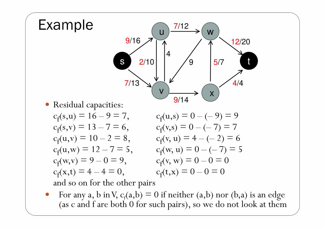
Example

s

v x

t

w u 9/16

7/12

12/20

2/10

4

9 5/7

4/4 7/13

9/14 y Residual capacities:

cf(s,u) = 16 – 9 = 7, cf(u,s�� ���– (– 9) = 9 cf(s,v) = 13 – 7 = 6, cf(v,s�� ���– (– 7) = 7 cf(u,v�� ����– 2 = 8, cf(v, u) = 4 – (– 2) = 6 cf(u,w) = 12 – 7 = 5, cf�Z��X�� ���– (– 7) = 5 cf(w,v) = 9 – �� ��������� cf�Y��Z�� ���– �� �� cf(x,t) = 4 – �� ���������� cf(t,x) = ��– �� ���� and so on for the other pairs

y For any a, b in V, cf(a,b�� ���LI�QHLWKHU��a,b) nor (b,a) is an edge �DV�F�DQG�I�DUH�ERWK���IRU�VXFK�SDLUV���VR�ZH�GR�QRW�ORRN�DW�WKHP

y 5HVLGXDO�*UDSK��HGJHV�ZLWK���UHVLGXDO�FDSDFLW\�DUH�QHYHU�VKRZQ�

y Note that residual graph may have edges where G did not (shown in color blue)

y It also may NOT have edges where G has one, ex. (x,t) y 7KH�UHVLGXDO�FDSDFLW\�RI�WKH�HGJH�LV�� y Such edges are called saturated

s

v x

t

w u

7

5 8

8

2

9 2

6

5

9

7

5

5

12

9

4

y Augmenting Path – path from s to t

y One path shown in bold grey, <s,u,w,t> with residual capacity = min(7, 5, 8) = 5 y We can increase (“augment”) the flow on each edge of the

path by 5 to get a new feasible flow with higher value

s

v x

t

w u

7

5 8

8

2

9 2

6

5

9

7

7

5

12

9

4

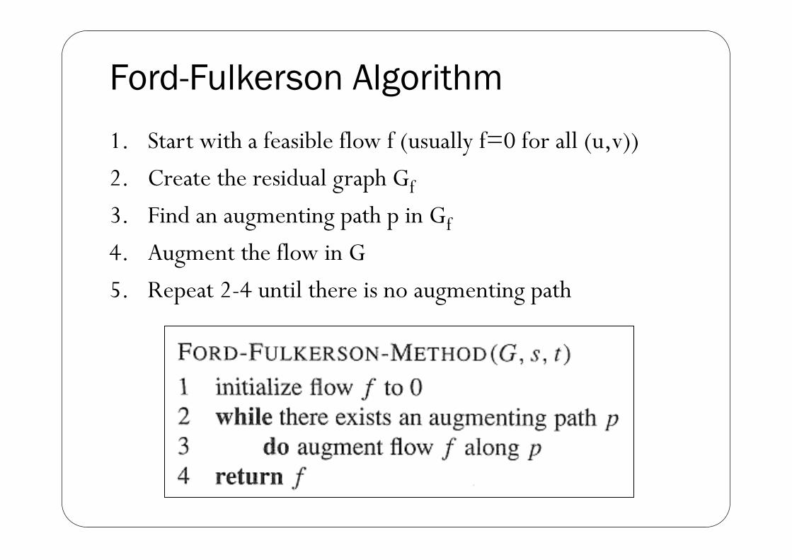
Ford-Fulkerson Algorithm

1. 6WDUW�ZLWK�D�IHDVLEOH�IORZ�I��XVXDOO\�I ��IRU�DOO��u,v))

2. Create the residual graph Gf

3. Find an augmenting path p in Gf

4. Augment the flow in G

5. Repeat 2-4 until there is no augmenting path

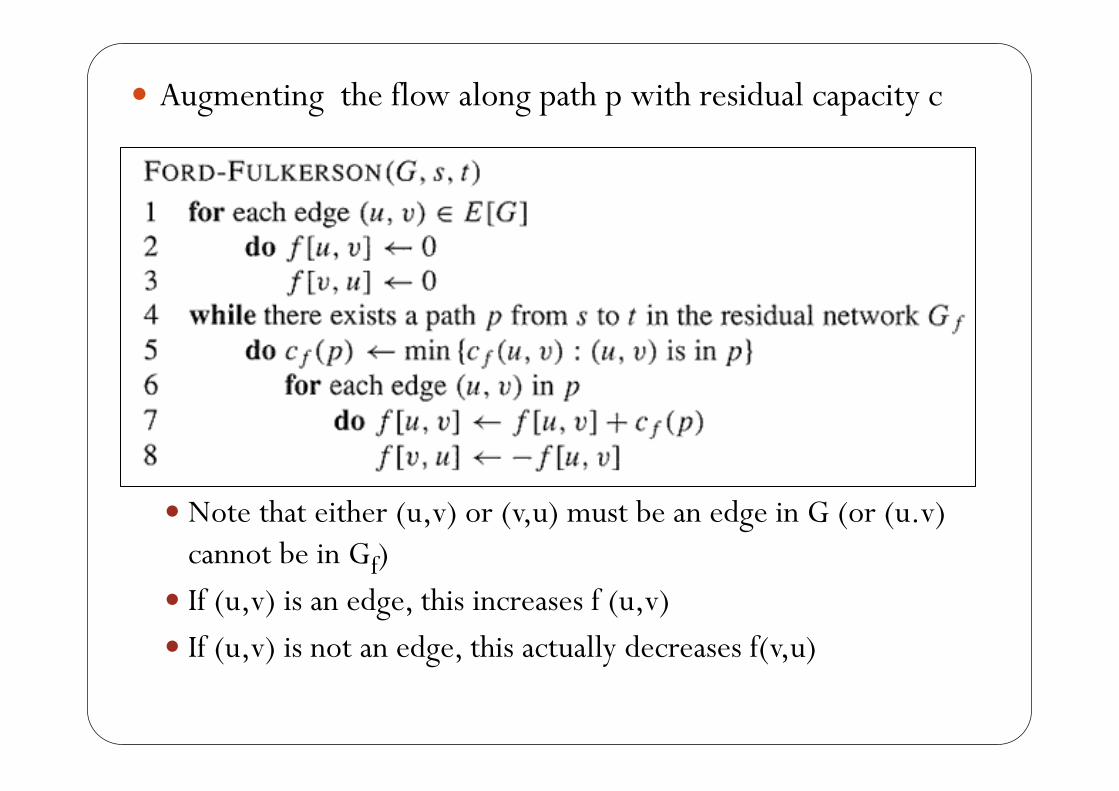
y Augmenting the flow along path p with residual capacity c

y Note that either (u,v) or (v,u) must be an edge in G (or (u.v)

cannot be in Gf)

y If (u,v) is an edge, this increases f (u,v)

y If (u,v) is not an edge, this actually decreases f(v,u)

s

v x

t

w u 4/16

4/12

0/20

10

4

4/9 7

4/4 0/13

4/14

s

v x

t

w u 11/16

4/12

7/20

7/1

0

4

4/9 7/7

4/4 13

11/14

s

v x

t

w u

16

12

20

10 4

9 7

4 13

14

s

v x

t

w u

12

8 20

10

4

5 7 13

10

4

4

4

4

4

Residual graph Flow Assignment

s

v x

t

w u 11/16

12/12

15/20

10

1/4

4/9 7/7

4/4 8/13

11/14

s

v x

t

w u 11/16

12/12

19/20

10

1/4

9 7/7

4/4 12/13

11/14

s

v x

t

w u

5

8 13

3

11

5 13

3

11

4

7 7

11

4 4

s

v x

t

w u

5

5

11

3

5

5

3

11

8

12

7 15

11

4 4

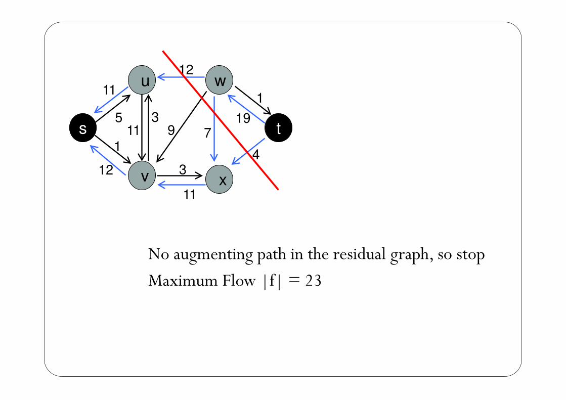
No augmenting path in the residual graph, so stop

Maximum Flow |f| = 23

s

v x

t

w u

5

1

11

3

9

1

3

11

12

12

7

19

11

4

Proof of Correctness

y We first need some definitions y A cut (S, T) of a flow network G = (V, E) is a partition of

V into S and T = V – S, such that s � S and t � T

y If f is a flow then the net flow across the cut (S, T) , f(S, T), is the sum of the flows (f) of all pairs (u,v) with u in S and v in T

y The capacity of the cut (S, T), c(S, T), is the sum of the capacities of all edges (u,v) with u in S and V in T

y 2I�FRXUVH��I�6��7����F�6��7�

y A minimum cut of a network is a cut whose capacity is minimum over all possible cuts of the network

y Consider the cut (S={s, u, v}, T={w, x, t})

y f(S, T) = f(u,w����I�v,w����I�v,x)

�������-�������� ���

y c(S, T) = c(u,w����F�v,x�� ��������� ���

s

v x

t

w u 10/16

8/12

12/20

2/10

4

1/9 5/7

5/5 7/13

10/14

Lemma 1: Let f be a flow in a network G with source s and sink t, and let (S, T) be a cut of G. Then the net flow across (S, T) is f(S, T) = |f|.

Proof:

f(S, T) = f(S,V) – f(S,S)

= f(S,V)

�I�V��9����f(S – s,V)

= f(s,V)

= |f|

Lemma 1 implies that the net flow across any cut is the same (= value of flow).

Corollary 2: The value of any flow f in a flow network G is bounded from above by the capacity of any cut of G, and hence by the capacity of the minimum cut.

Theorem 3 (Max-flow min-cut theorem): If f is a flow in a flow network G = (V, E) with source s and sink t, then the following conditions are equivalent:

1. f is a maximum flow in G

2. The residual network Gf contains no augmenting paths

3. |f| = capacity of the minimum cut

Proof:

1 implies 2 is obvious, as otherwise |f| can be increased by increasing the flow along the augmenting path

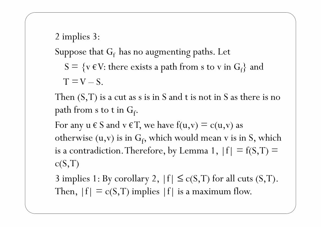
2 implies 3:

Suppose that Gf has no augmenting paths. Let

S = {v € V: there exists a path from s to v in Gf} and

T = V – S.

Then (S,T) is a cut as s is in S and t is not in S as there is no path from s to t in Gf.

For any u € S and v € T, we have f(u,v) = c(u,v) as otherwise (u,v) is in Gf, which would mean v is in S, which is a contradiction. Therefore, by Lemma 1, |f| = f(S,T) = c(S,T)

3 implies 1: By corollary 2, |f| ��F�6�7��for all cuts (S,T). Then, |f| = c(S,T) implies |f| is a maximum flow.

Time Complexity

y Original Ford-Fulkerson algorithm does not specify how to find an augmenting path y Can find in any order

y Assume all capacities are integer y Let f* = maximum flow y Lines 1-3 (Initialization) takes O(|E|) time y No. of times the while loop (no. of times an augmenting path

is found) is executed is bounded above by |f*| y As |f| increases by at least 1 in each augmentation

y Each iteration of the while loop takes O(|E|) time y So worst case time complexity O(|E||f*|)

y This is not polynomial, it is pseudo-polynomial

y This bound is tight