Embed Size (px)
Citation preview
netfabb Professional 6.0 and
netfabb Enterprise 6.0
User manual
Copyright by netfabb GmbH 2010
Version: June 01, 2015
This document shall not be distributed without the permission of netfabb GmbH.
2
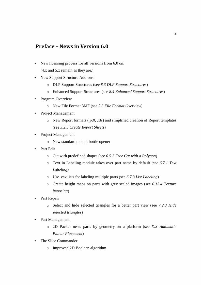
Preface – News in Version 6.0
• New licensing process for all versions from 6.0 on.
(4.x and 5.x remain as they are.)
• New Support Structure Add-ons:
o DLP Support Structures (see 8.3 DLP Support Structures)
o Enhanced Support Structures (see 8.4 Enhanced Support Structures)
• Program Overview
o New File Format 3MF (see 2.5 File Format Overview)
• Project Management
o New Report formats (.pdf, .xls) and simplified creation of Report templates
(see 3.2.5 Create Report Sheets)
• Project Management
o New standard model: bottle opener
• Part Edit
o Cut with predefined shapes (see 6.5.2 Free Cut with a Polygon)
o Text in Labeling module takes over part name by default (see 6.7.1 Text
Labeling)
o Use .csv lists for labeling multiple parts (see 6.7.3 List Labeling)
o Create height maps on parts with grey scaled images (see 6.13.4 Texture
imposing)
• Part Repair
o Select and hide selected triangles for a better part view (see 7.2.3 Hide
selected triangles)
• Part Management
o 2D Packer nests parts by geometry on a platform (see X.X Automatic
Planar Placement)
• The Slice Commander
o Improved 2D Boolean algorithm
3
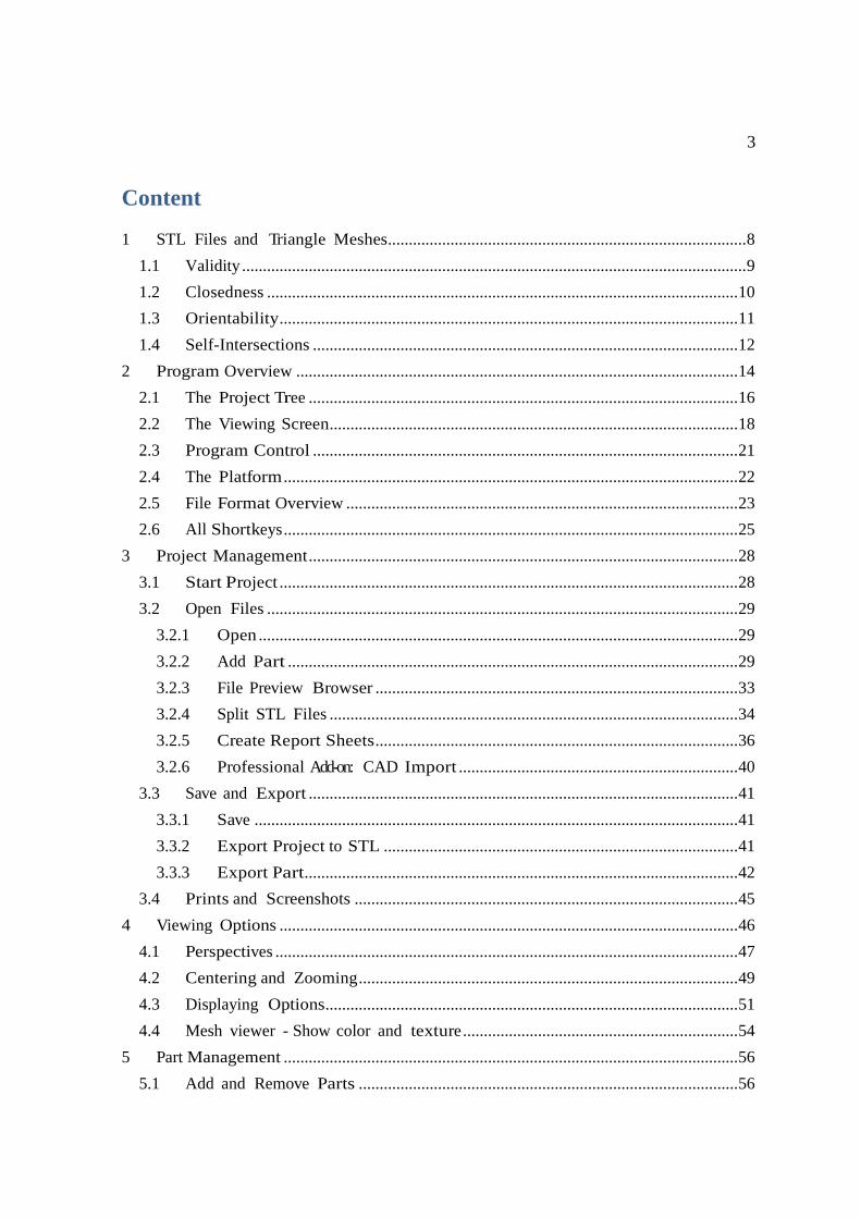
Content 1 STL Files and Triangle Meshes ...................................................................................... 8
1.1 Validity ......................................................................................................................... 9
1.2 Closedness ................................................................................................................. 10
1.3 Orientability .............................................................................................................. 11
1.4 Self-Intersections ...................................................................................................... 12
2 Program Overview .......................................................................................................... 14
2.1 The Project Tree ....................................................................................................... 16
2.2 The Viewing Screen.................................................................................................. 18
2.3 Program Control ...................................................................................................... 21
2.4 The Platform ............................................................................................................. 22
2.5 File Format Overview .............................................................................................. 23
2.6 All Shortkeys ............................................................................................................. 25
3 Project Management ....................................................................................................... 28
3.1 Start Project .............................................................................................................. 28
3.2 Open Files ................................................................................................................. 29
3.2.1 Open ................................................................................................................... 29
3.2.2 Add Part ............................................................................................................ 29
3.2.3 File Preview Browser ....................................................................................... 33
3.2.4 Split STL Files .................................................................................................. 34
3.2.5 Create Report Sheets ....................................................................................... 36
3.2.6 Professional Add-on: CAD Import ................................................................... 40
3.3 Save and Export ....................................................................................................... 41
3.3.1 Save .................................................................................................................... 41
3.3.2 Export Project to STL ..................................................................................... 41
3.3.3 Export Part........................................................................................................ 42
3.4 Prints and Screenshots ............................................................................................ 45
4 Viewing Options .............................................................................................................. 46
4.1 Perspectives ............................................................................................................... 47
4.2 Centering and Zooming ........................................................................................... 49
4.3 Displaying Options ................................................................................................... 51
4.4 Mesh viewer - Show color and texture .................................................................. 54
5 Part Management ............................................................................................................. 56
5.1 Add and Remove Parts ........................................................................................... 56
4
5.2 Select Parts ................................................................................................................ 56
5.2.1 Advanced Part Selection .................................................................................. 58
5.3 Standard models - the part library ......................................................................... 60
5.4 Duplicate Parts .......................................................................................................... 63
5.5 Position and Scale .................................................................................................... 65
5.5.1 Move Parts ........................................................................................................ 65
5.5.2 Rotate Parts ........................................................................................................ 66
5.5.3 Align Parts......................................................................................................... 67
5.5.4 Scale Parts ......................................................................................................... 70
5.5.5 Arrange Parts .................................................................................................... 71
5.6 Automatic planar placement ....................................................................................... 72
5.7 Part Attributes ........................................................................................................... 76
5.8 Platform Overview ................................................................................................... 78
5.9 New platform ............................................................................................................ 79
5.10 Collision Detection ............................................................................................... 79
5.10.1 Live Collision Detection................................................................................... 81
5.11 Professional / Enterprise Add-On: Automatic Packing in 3D build volume .......... 83
5.11.1 Small .................................................................................................................. 83
5.11.2 Medium and Large........................................................................................... 85
6 Part Edit ............................................................................................................................ 87
6.1 Part Analysis .............................................................................................................. 87
6.1.1 Standard Analysis ............................................................................................ 89
6.1.2 Upskin and Downskin Analysis ....................................................................... 89
6.1.3 Center of gravity ............................................................................................... 90
6.1.4 Wall thickness ................................................................................................... 91
6.1.5 Shadow Area Analysis ..................................................................................... 92
6.2 Simple Part Editing ................................................................................................... 92
6.2.1 Invert Part ......................................................................................................... 93
6.2.2 Mirror ................................................................................................................ 93
6.2.3 Convert Units .................................................................................................... 94
6.2.4 Shells to Parts ................................................................................................... 95
6.2.5 Merge Parts ....................................................................................................... 95
6.3 Create Shell............................................................................................................... 95
6.4 Simple Cutting .......................................................................................................... 98
5
6.5 Free Cut .................................................................................................................. 102
6.5.1 Free Cut with a Cutting Plane ..................................................................... 102
6.5.2 Free Cut with a Polygon ................................................................................ 108
6.5.3 Cutting Options .............................................................................................. 115
6.6 Boolean Operations ................................................................................................ 117
6.7 Labeling ................................................................................................................... 120
6.7.1 Text labeling ..................................................................................................... 120
6.7.2 Image labeling ................................................................................................. 121
6.7.3 List labeling ...................................................................................................... 124
6.8 Triangle Reduction ................................................................................................. 129
6.9 Mesh Smoothing ..................................................................................................... 129
6.10 Remesh ................................................................................................................. 131
6.11 Compare two meshes .......................................................................................... 133
6.12 Windows R
Kinect R
scan to netfabb ................................................................... 137
6.13 Color and texture .................................................................................................. 138
6.13.1 Coloring ........................................................................................................... 138
6.13.2 Texturing ......................................................................................................... 140
6.13.3 Add advanced texture .................................................................................... 142
6.13.4 Texture imposing .............................................................................................. 146
7 Part Repair ...................................................................................................................... 148
7.1 The Repair Module ................................................................................................. 148
7.2 Repair Viewing Options .......................................................................................... 150
7.2.1 Zoom and visualization ................................................................................. 150
7.2.2 Inner view ....................................................................................................... 151
7.2.3 Hide selected surfaces ....................................................................................... 152
7.3 Selection ................................................................................................................... 153
7.4 Manual Repair ........................................................................................................ 158
7.5 Semi-Automatic Repair .......................................................................................... 161
7.5.1 Close Holes ...................................................................................................... 162
7.5.2 Self-Intersections .............................................................................................. 163
7.5.3 Stitch Triangles ............................................................................................... 165
7.5.4 Fix Flipped Triangles ...................................................................................... 165
7.5.5 Remove Double Triangles.............................................................................. 166
7.5.6 Select Overlapping Triangles ........................................................................ 167
6
7.5.7 Remove Degenerate Faces ............................................................................. 167
7.5.8 Extract Selected Triangles As Part .............................................................. 168
7.5.9 Split Non-Oriented Edges ............................................................................. 169
7.5.10 Wrap part surface ......................................................................................... 169
7.6 Automatic Repair ................................................................................................... 170
7.7 Edit Triangle Mesh ................................................................................................ 172
7.7.1 Refine Triangle Mesh ....................................................................................... 172
7.7.2 Reduce Triangles ............................................................................................ 173
7.7.3 Z-Compensation ............................................................................................. 174
7.7.4 Smooth Triangles ............................................................................................. 175
7.7.5 Cut Surfaces .................................................................................................... 177
7.7.6 Offset Hole Edges ........................................................................................... 179
7.7.7 Extrude Surfaces ............................................................................................ 180
7.7.8 3D-Extrude ...................................................................................................... 184
8 Support Structures (Professional / Enterprise Add-on) ................................................... 233
8.1 General Settings ........................................................................................................ 234
8.2 Downskin analysis .................................................................................................... 236
8.3 DLP Support Module ............................................................................................... 237
8.3.1 Manual Support Creation .................................................................................. 238
8.3.2 Semiautomatic Support Creation ...................................................................... 242
8.3.3 Automatic Support ............................................................................................ 243
8.4 Enhanced Support Structures ................................................................................... 246
8.4.1 Manual support creation ................................................................................... 247
8.4.2 Semiautomatic Support Creation ...................................................................... 258
8.4.3 Automatic Support ............................................................................................ 259
9 Measuring and Quality Assurance ............................................................................ 268
9.1 The Measuring Tool ............................................................................................... 268
9.1.1 Cutting Lines .................................................................................................. 271
9.1.2 Setting Anchors .............................................................................................. 271
9.1.3 Measure Distance ........................................................................................... 273
9.1.4 Measure Angles .............................................................................................. 275
9.1.5 Measure Radius .............................................................................................. 276
9.1.6 Add Note .......................................................................................................... 276
9.1.7 Set Default Modes .......................................................................................... 277
7
9.1.8 Lock and Unlock View .................................................................................. 278
9.2 Test ........................................................................................................................... 279
9.2.1 Create Definition ............................................................................................ 280
9.2.2 Values ............................................................................................................... 281
9.2.3 Test Result ....................................................................................................... 281
10 The Slice Commander .................................................................................................. 282
10.1 The Slicing Process ............................................................................................. 282
10.2 The Slices Section ............................................................................................... 283
10.3 Active Slice File ................................................................................................... 284
10.4 Slice Selection and Handling ............................................................................ 285
10.4.1 Select Slices ..................................................................................................... 285
10.4.2 Slice Viewing Options .................................................................................... 286
10.4.3 Move, Rotate, Scale and Mirror Slices ........................................................ 288
10.4.4 Merging and Grouping ................................................................................... 291
10.5 Edit Slices ............................................................................................................ 291
10.5.1 Boolean Operations & Removing Self-Intersections .................................. 292
10.5.2 Create Offsets of Slices .................................................................................. 294
10.5.3 Point Reduction .............................................................................................. 296
10.6 Edit Filling .......................................................................................................... 297
10.6.1 Create Filling .................................................................................................. 297
10.6.2 Hatch cutting .................................................................................................... 300
10.6.3 Convert contours/hatches .............................................................................. 301
10.7 Export and Save Slices ........................................................................................ 302
11 Settings ........................................................................................................................... 313
11.1 General Settings ................................................................................................. 313
11.2 Change Colors .................................................................................................... 319
11.3 Edit File Associations ......................................................................................... 322
12 Appendix ......................................................................................................................... 323
12.1 Image field parameters ......................................................................................... 323
12.2 Text field parameters ............................................................................................ 323

8
1 STL Files and Triangle Meshes
The STL-format is the industrial standard for handling triangulated meshes. STL-files
contain a plain list of three-dimensional corner point coordinates and flat triangles. The
triangles, also referred to as faces, are defined by three corner points and have an inside
and an outside. Adjacent triangles may use common corner points and share the same
edges, which results in a coherent triangle mesh (figure 1.1). The generality and
simplicity of this concept makes STL-files compatible to a lot of applications.
Figure 1.1: Parametric Surface and Triangulated Representation
However, they do not contain any topological information about the mesh. This causes
typical errors when CAD files with different file formats are converted to STL. The
netfabb software is a specialized software to detect and repair these kinds of damages and
create faultless meshes without holes, deformations or intersections.
These meshes can then be converted into slice files ready for additive manufacturing. The
STL format aims for a precise approximation of bodies in three-dimensional space.
Although other CAD formats have advantages in that respect, a variety of applications
need a surface representation consisting of flat triangles. These are:
o Accelerated rendering in multimedia applications
o Solving partial differential equations
9
o Computer aided engineering
o Rapid prototyping and additive manufacturing However, a simple collection of triangles will not always create a solid body. For a good
triangle mesh that can be used for 3D printing, the mesh has to be valid, closed, oriented
and should not contain any self-intersections.
1.1 Validity
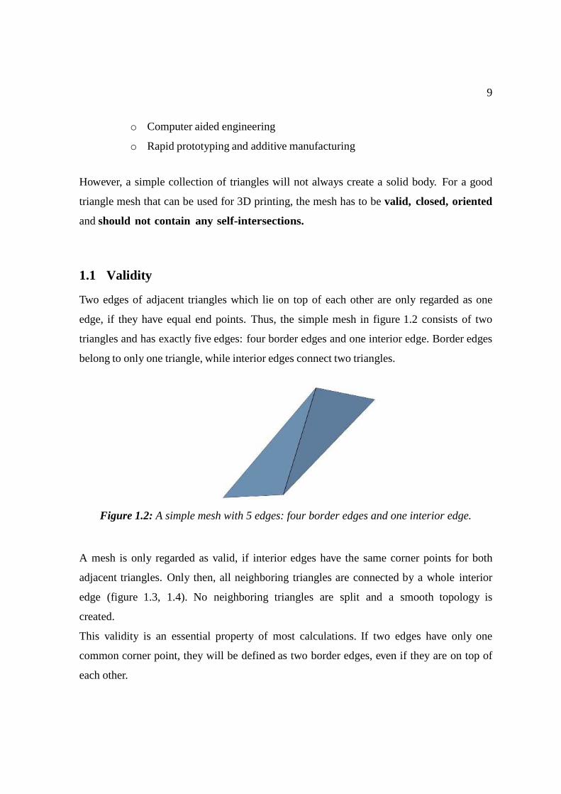
Two edges of adjacent triangles which lie on top of each other are only regarded as one
edge, if they have equal end points. Thus, the simple mesh in figure 1.2 consists of two
triangles and has exactly five edges: four border edges and one interior edge. Border edges
belong to only one triangle, while interior edges connect two triangles.
Figure 1.2: A simple mesh with 5 edges: four border edges and one interior edge.
A mesh is only regarded as valid, if interior edges have the same corner points for both
adjacent triangles. Only then, all neighboring triangles are connected by a whole interior
edge (figure 1.3, 1.4). No neighboring triangles are split and a smooth topology is
created.
This validity is an essential property of most calculations. If two edges have only one
common corner point, they will be defined as two border edges, even if they are on top of
each other.
10
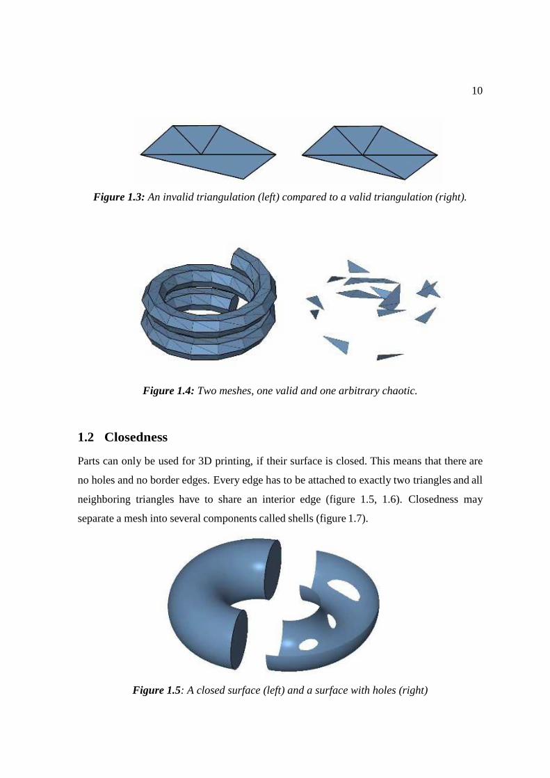
Figure 1.3: An invalid triangulation (left) compared to a valid triangulation (right).
Figure 1.4: Two meshes, one valid and one arbitrary chaotic.
1.2 Closedness
Parts can only be used for 3D printing, if their surface is closed. This means that there are
no holes and no border edges. Every edge has to be attached to exactly two triangles and all
neighboring triangles have to share an interior edge (figure 1.5, 1.6). Closedness may
separate a mesh into several components called shells (figure 1.7).
Figure 1.5: A closed surface (left) and a surface with holes (right)
11
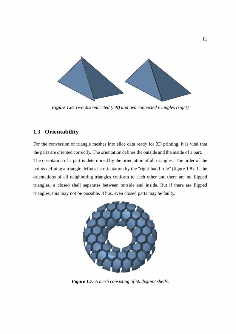
Figure 1.6: Two disconnected (left) and two connected triangles (right)
1.3 Orientability
For the conversion of triangle meshes into slice data ready for 3D printing, it is vital that
the parts are oriented correctly. The orientation defines the outside and the inside of a part.
The orientation of a part is determined by the orientation of all triangles. The order of the
points defining a triangle defines its orientation by the "right-hand-rule" (figure 1.8). If the
orientations of all neighboring triangles conform to each other and there are no flipped
triangles, a closed shell separates between outside and inside. But if there are flipped
triangles, this may not be possible. Thus, even closed parts may be faulty.
Figure 1.7: A mesh consisting of 60 disjoint shells.
12
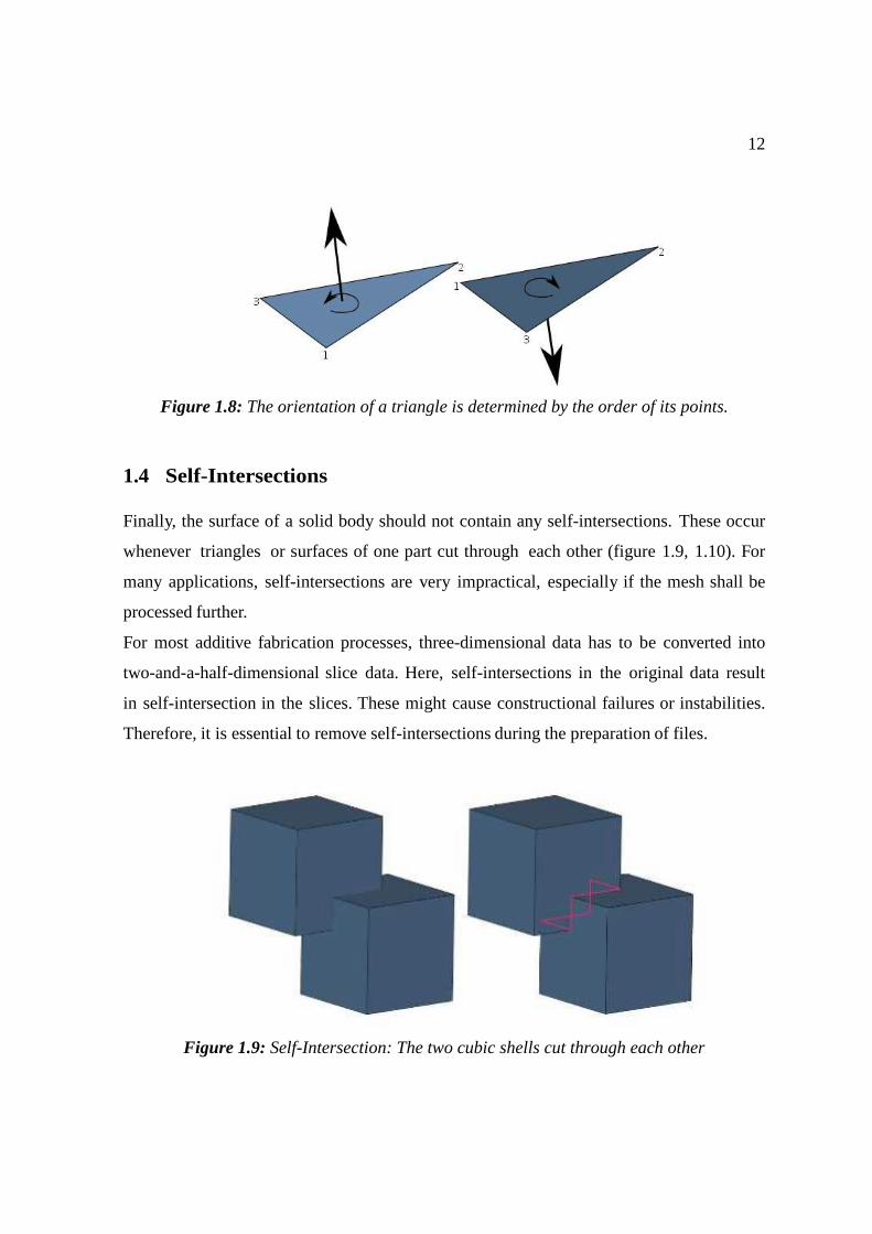
Figure 1.8: The orientation of a triangle is determined by the order of its points.
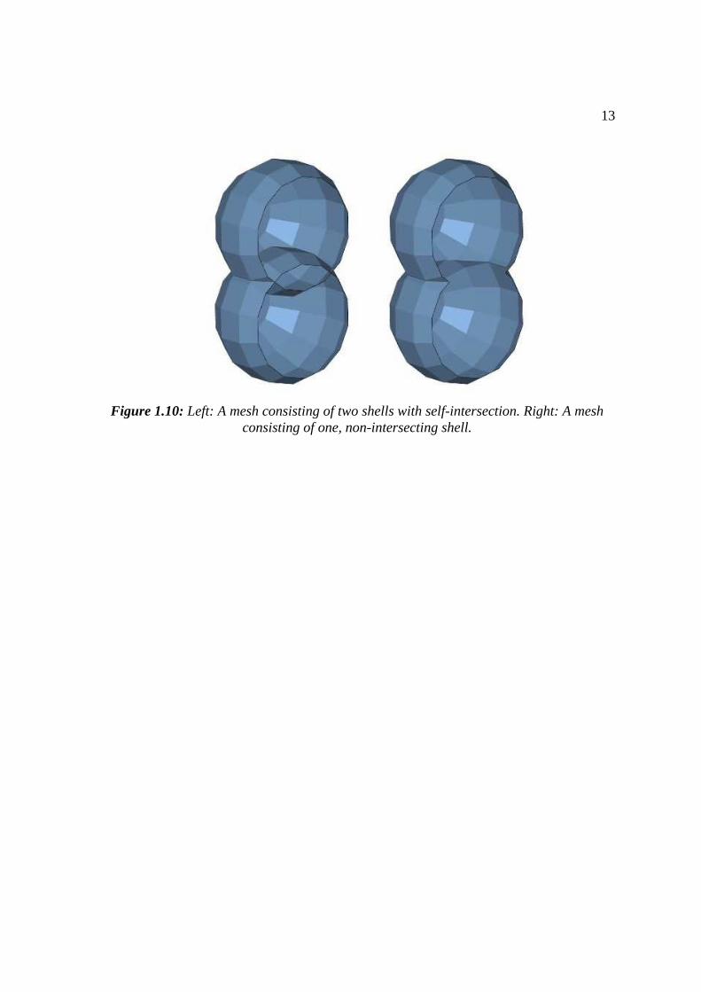
1.4 Self-Intersections
Finally, the surface of a solid body should not contain any self-intersections. These occur
whenever triangles or surfaces of one part cut through each other (figure 1.9, 1.10). For
many applications, self-intersections are very impractical, especially if the mesh shall be
processed further.
For most additive fabrication processes, three-dimensional data has to be converted into
two-and-a-half-dimensional slice data. Here, self-intersections in the original data result
in self-intersection in the slices. These might cause constructional failures or instabilities.
Therefore, it is essential to remove self-intersections during the preparation of files.
Figure 1.9: Self-Intersection: The two cubic shells cut through each other
13
Figure 1.10: Left: A mesh consisting of two shells with self-intersection. Right: A mesh consisting of one, non-intersecting shell.
14
2 Program Overview
netfabb is a software tailored for additive manufacturing, rapid prototyping and 3D
printing. It prepares three-dimensional files for printing and converts them into two-and-a-
half-dimensional slice files, consisting of a list of two-dimensional slice layers. To help users
prepare the print, it includes the features for viewing, editing, repairing and analyzing three-
dimensional STL-files or slice-based files in various formats.
All operations are conducted within projects, which can include any number of three-
dimensional parts or slice files. The modular design of the software allows the use of
different modules within a project, such as the repair module or the Slice Commander,
which are linked to other user interfaces. Still, they can be executed simultaneously, as the
user can switch between modules without any loss of information.
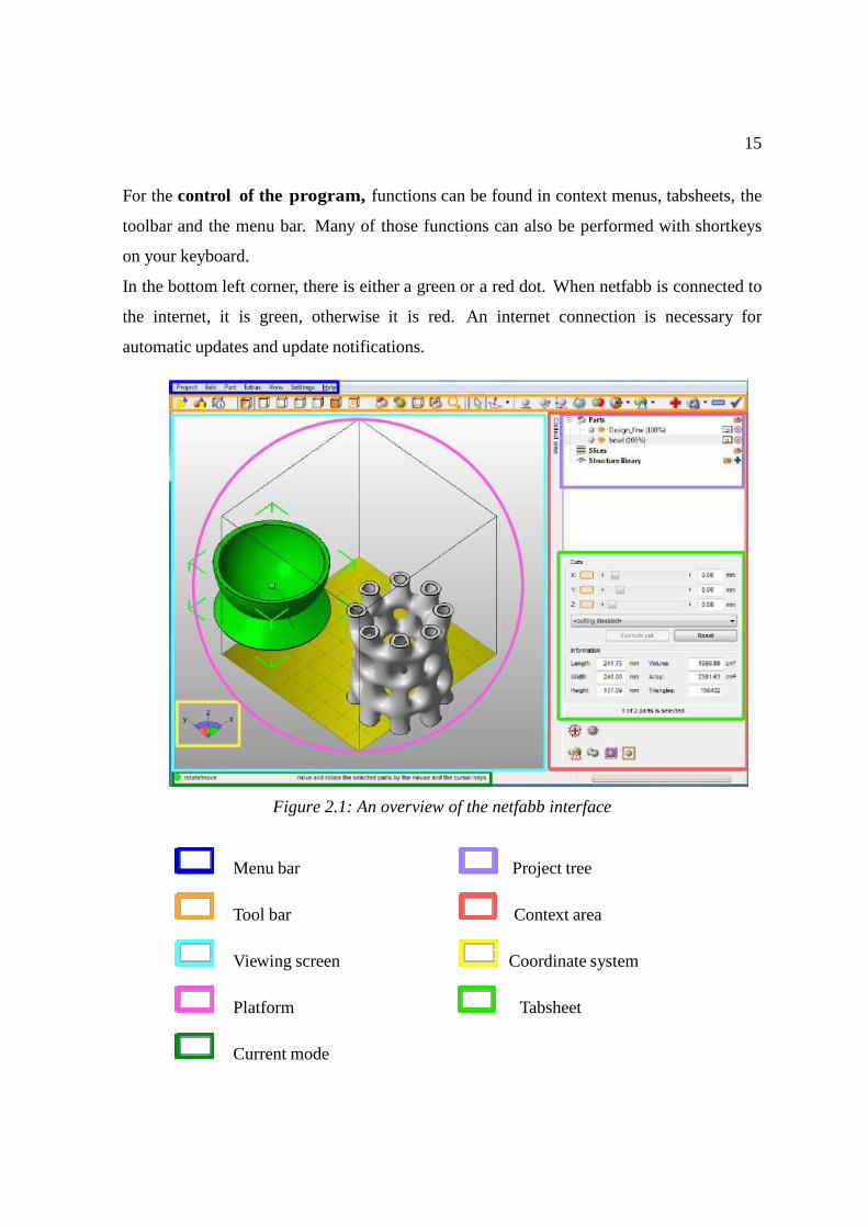
The user interface of the program is divided into the viewing screen, the menu bar and
toolbar at the top and the context area to the right (figure 2.1). By clicking on the bar
between the viewing screen and the context area, the context area is hidden and the bar is
pushed to the right edge of the screen. Another click on the bar will bring the context area
back. By clicking on the edge of the bar and holding the mouse button, you can move the
edge further into the screen by drag & drop.
In the top half of the context area, all parts and slices are listed in the project tree. The
project tree can be used to get an overview over the project, organize files and to perform
certain functions.
Most of the netfabb window however is occupied by the viewing screen, which
visualizes the project and includes viewing options, positioning functions and a few basic
handling options.
15
For the control of the program, functions can be found in context menus, tabsheets, the
toolbar and the menu bar. Many of those functions can also be performed with shortkeys
on your keyboard.
In the bottom left corner, there is either a green or a red dot. When netfabb is connected to
the internet, it is green, otherwise it is red. An internet connection is necessary for
automatic updates and update notifications.
Figure 2.1: An overview of the netfabb interface
Menu bar Project tree
Tool bar Context area
Viewing screen Coordinate system
Platform Tabsheet
Current mode
16
2.1 The Project Tree
The project tree lists all parts and slices of a project in a way similar to a directory
tree. There are several sections, such as "Parts" and "Slices". The elements in the project
tree can be sorted into groups, and they can have subordinate elements, such as a part
repair or the measuring of a part. These are often connected to other modules.
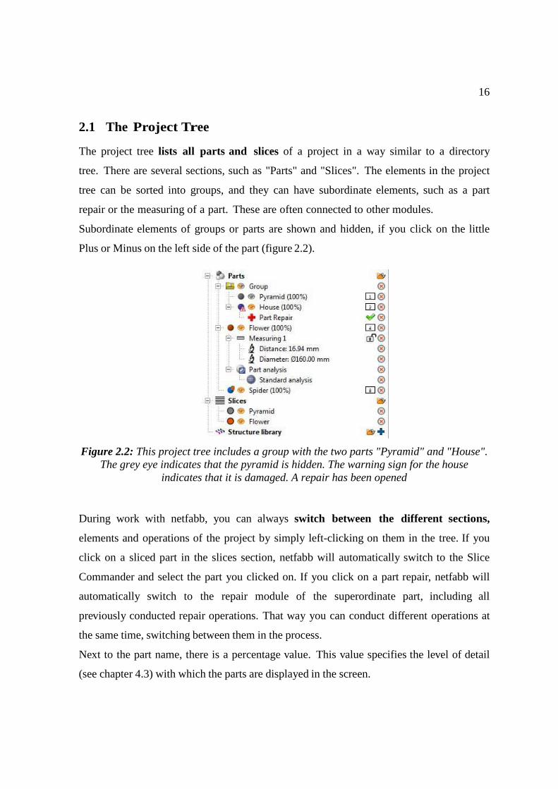
Subordinate elements of groups or parts are shown and hidden, if you click on the little
Plus or Minus on the left side of the part (figure 2.2).
Figure 2.2: This project tree includes a group with the two parts "Pyramid" and "House". The grey eye indicates that the pyramid is hidden. The warning sign for the house
indicates that it is damaged. A repair has been opened
During work with netfabb, you can always switch between the different sections,
elements and operations of the project by simply left-clicking on them in the tree. If you
click on a sliced part in the slices section, netfabb will automatically switch to the Slice
Commander and select the part you clicked on. If you click on a part repair, netfabb will
automatically switch to the repair module of the superordinate part, including all
previously conducted repair operations. That way you can conduct different operations at
the same time, switching between them in the process.
Next to the part name, there is a percentage value. This value specifies the level of detail
(see chapter 4.3) with which the parts are displayed in the screen.
17
By clicking on parts or slices, these are selected and can be worked with. If a part is
selected and you hold Shift and click on another part, all parts on the list between the first
selected part and the part you clicked on are selected. By holding Ctrl and clicking on
parts, those are either added to or removed from the selection.
When a part is damaged (inverted triangles or open triangle edges) or consists of more
than one shell, you can see that immediately in the project tree. Damaged parts have a small
caution sign at the bottom right of the colored dot next to the part name. Parts with more
than one shell have a little box at the top right of the dot.
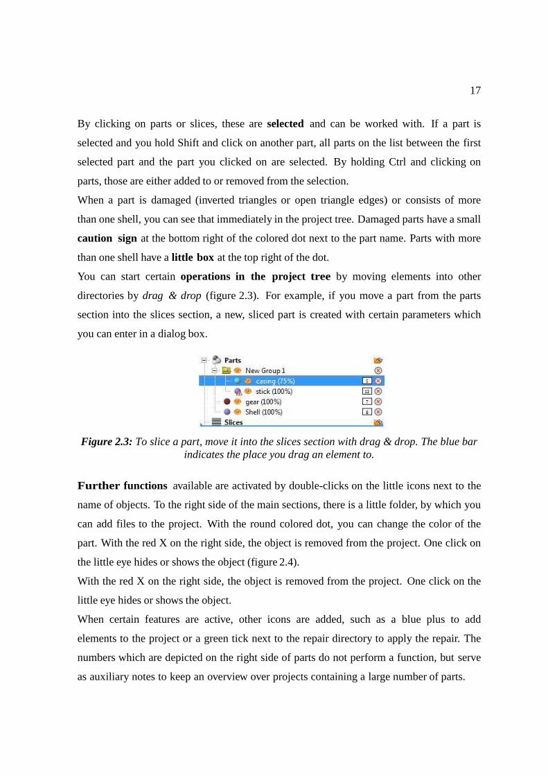
You can start certain operations in the project tree by moving elements into other
directories by drag & drop (figure 2.3). For example, if you move a part from the parts
section into the slices section, a new, sliced part is created with certain parameters which
you can enter in a dialog box.
Figure 2.3: To slice a part, move it into the slices section with drag & drop. The blue bar indicates the place you drag an element to.
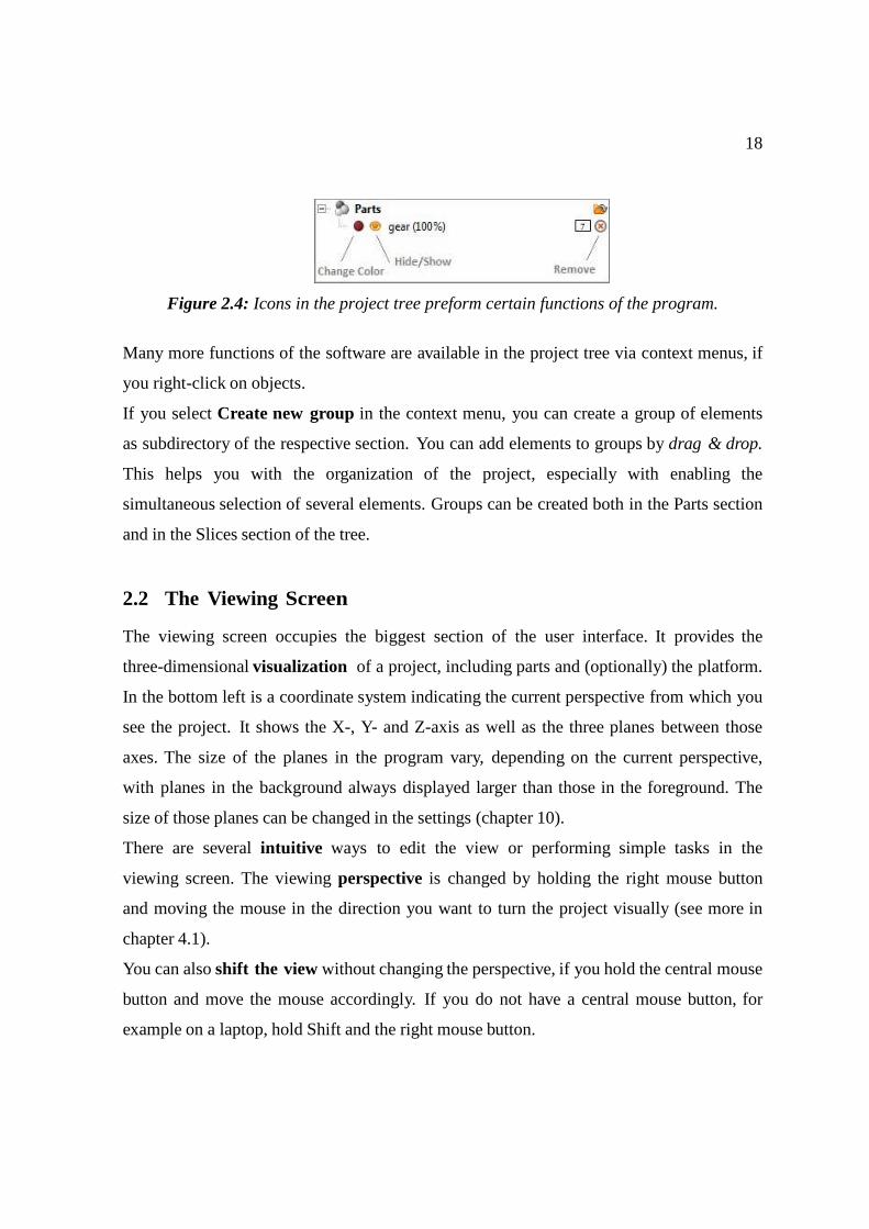
Further functions available are activated by double-clicks on the little icons next to the
name of objects. To the right side of the main sections, there is a little folder, by which you
can add files to the project. With the round colored dot, you can change the color of the
part. With the red X on the right side, the object is removed from the project. One click on
the little eye hides or shows the object (figure 2.4).
With the red X on the right side, the object is removed from the project. One click on the
little eye hides or shows the object.
When certain features are active, other icons are added, such as a blue plus to add
elements to the project or a green tick next to the repair directory to apply the repair. The
numbers which are depicted on the right side of parts do not perform a function, but serve
as auxiliary notes to keep an overview over projects containing a large number of parts.
18
Figure 2.4: Icons in the project tree preform certain functions of the program.
Many more functions of the software are available in the project tree via context menus, if
you right-click on objects.
If you select Create new group in the context menu, you can create a group of elements
as subdirectory of the respective section. You can add elements to groups by drag & drop.
This helps you with the organization of the project, especially with enabling the
simultaneous selection of several elements. Groups can be created both in the Parts section
and in the Slices section of the tree.
2.2 The Viewing Screen
The viewing screen occupies the biggest section of the user interface. It provides the
three-dimensional visualization of a project, including parts and (optionally) the platform.
In the bottom left is a coordinate system indicating the current perspective from which you
see the project. It shows the X-, Y- and Z-axis as well as the three planes between those
axes. The size of the planes in the program vary, depending on the current perspective,
with planes in the background always displayed larger than those in the foreground. The
size of those planes can be changed in the settings (chapter 10).
There are several intuitive ways to edit the view or performing simple tasks in the
viewing screen. The viewing perspective is changed by holding the right mouse button
and moving the mouse in the direction you want to turn the project visually (see more in
chapter 4.1).
You can also shift the view without changing the perspective, if you hold the central mouse
button and move the mouse accordingly. If you do not have a central mouse button, for
example on a laptop, hold Shift and the right mouse button.
19
To zoom in or out use the scroll button of your mouse. If you do not have a scroll button,
hold Ctrl and the right mouse button and move the mouse up and down (figure 2.7, see
more in chapter 4.2).
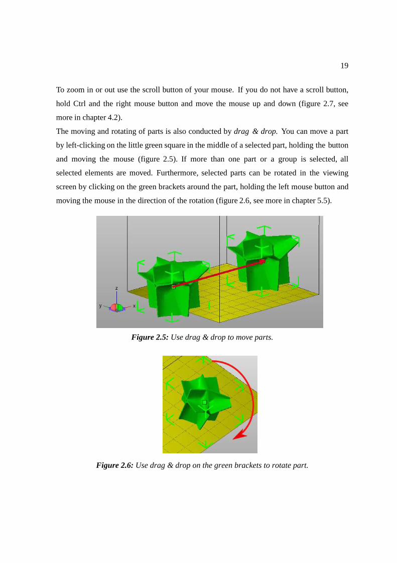
The moving and rotating of parts is also conducted by drag & drop. You can move a part
by left-clicking on the little green square in the middle of a selected part, holding the button
and moving the mouse (figure 2.5). If more than one part or a group is selected, all
selected elements are moved. Furthermore, selected parts can be rotated in the viewing
screen by clicking on the green brackets around the part, holding the left mouse button and
moving the mouse in the direction of the rotation (figure 2.6, see more in chapter 5.5).
Figure 2.5: Use drag & drop to move parts.
Figure 2.6: Use drag & drop on the green brackets to rotate part.
20
Figure 2.7: Change perspective and zoom with right mouse button and scroll button.
Below the screen, the current mode is specified, indicating which intuitive operation can
currently be conducted with the mouse (default: Move/Rotate). If you change the mode, for
example to "Align to Bottom Plane", other operations can be performed by the mouse (in
this case a double-click on a surface of a part rotates the part to align that surface to the X-
Y-plane).
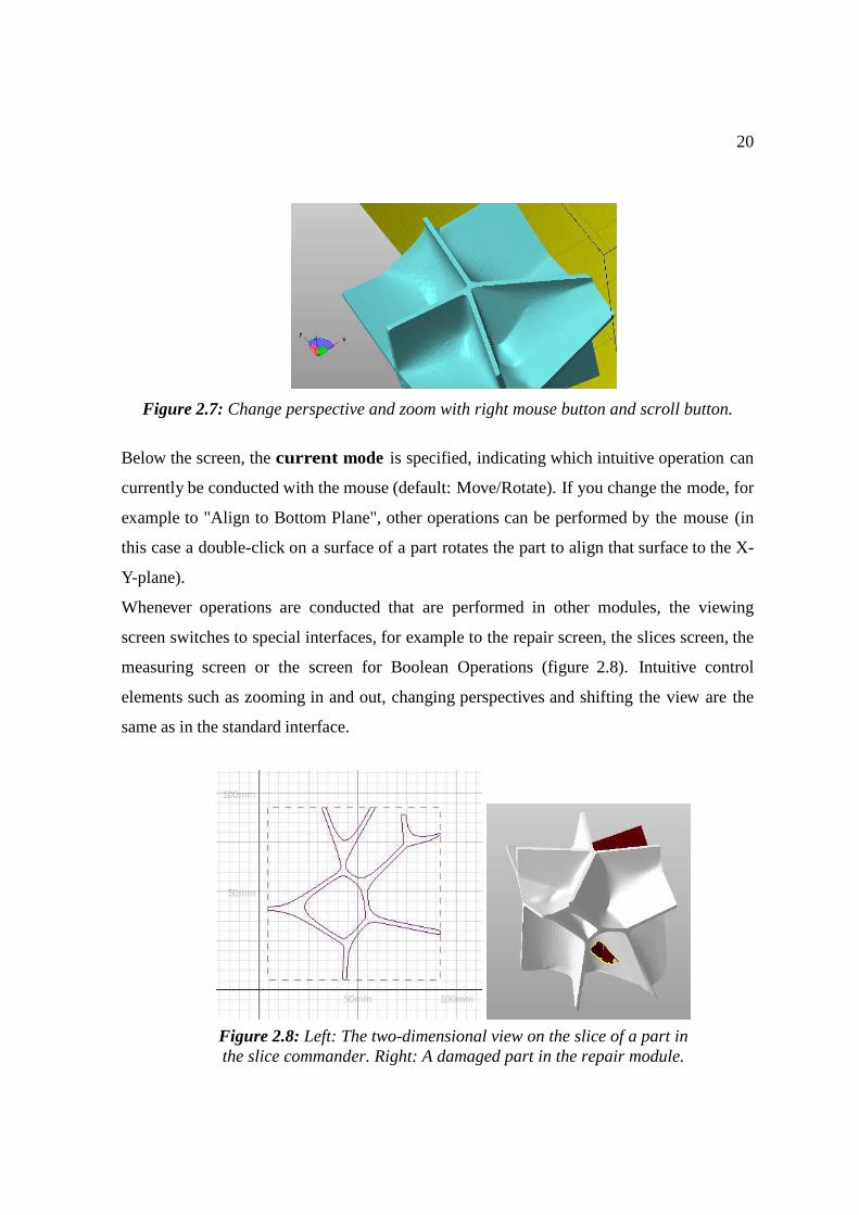
Whenever operations are conducted that are performed in other modules, the viewing
screen switches to special interfaces, for example to the repair screen, the slices screen, the
measuring screen or the screen for Boolean Operations (figure 2.8). Intuitive control
elements such as zooming in and out, changing perspectives and shifting the view are the
same as in the standard interface.
Figure 2.8: Left: The two-dimensional view on the slice of a part in the slice commander. Right: A damaged part in the repair module.
21
2.3 Program Control
Apart from these intuitive handling elements in the viewing screen (as described above),
there are several ways to use the program’s functionality, as most features can be found in
several places.
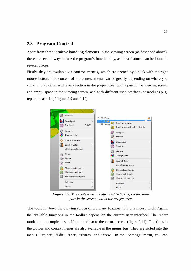
Firstly, they are available via context menus, which are opened by a click with the right
mouse button. The content of the context menus varies greatly, depending on where you
click. It may differ with every section in the project tree, with a part in the viewing screen
and empty space in the viewing screen, and with different user interfaces or modules (e.g.
repair, measuring / figure 2.9 and 2.10).
The toolbar above the viewing screen offers many features with one mouse click. Again,
the available functions in the toolbar depend on the current user interface. The repair
module, for example, has a different toolbar to the normal screen (figure 2.11). Functions in
the toolbar and context menus are also available in the menu bar. They are sorted into the
menus "Project", "Edit", "Part", "Extras" and "View". In the "Settings" menu, you can
Figure 2.9: The context menus after right-clicking on the same part in the screen and in the project tree.
22
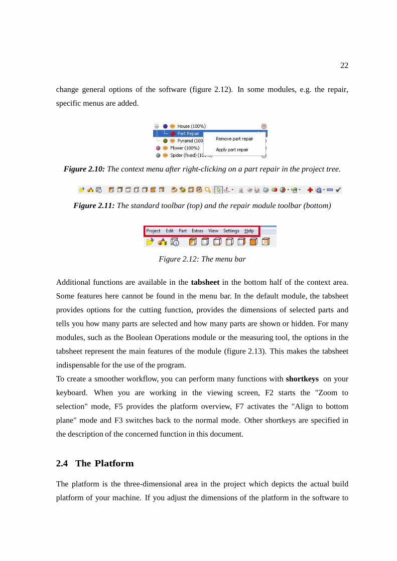
change general options of the software (figure 2.12). In some modules, e.g. the repair,
specific menus are added.
Figure 2.10: The context menu after right-clicking on a part repair in the project tree.
Figure 2.11: The standard toolbar (top) and the repair module toolbar (bottom)
Figure 2.12: The menu bar
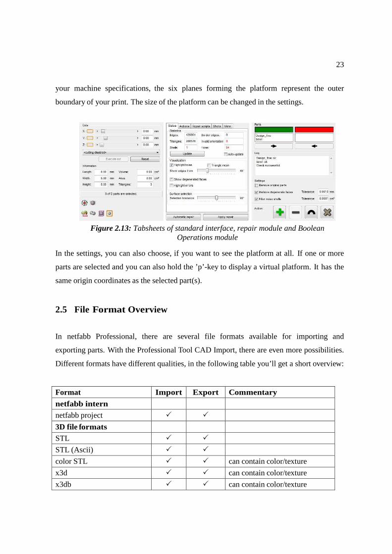
Additional functions are available in the tabsheet in the bottom half of the context area.
Some features here cannot be found in the menu bar. In the default module, the tabsheet
provides options for the cutting function, provides the dimensions of selected parts and
tells you how many parts are selected and how many parts are shown or hidden. For many
modules, such as the Boolean Operations module or the measuring tool, the options in the
tabsheet represent the main features of the module (figure 2.13). This makes the tabsheet
indispensable for the use of the program.
To create a smoother workflow, you can perform many functions with shortkeys on your
keyboard. When you are working in the viewing screen, F2 starts the "Zoom to
selection" mode, F5 provides the platform overview, F7 activates the "Align to bottom
plane" mode and F3 switches back to the normal mode. Other shortkeys are specified in
the description of the concerned function in this document.
2.4 The Platform
The platform is the three-dimensional area in the project which depicts the actual build
platform of your machine. If you adjust the dimensions of the platform in the software to
23
your machine specifications, the six planes forming the platform represent the outer
boundary of your print. The size of the platform can be changed in the settings.
In the settings, you can also choose, if you want to see the platform at all. If one or more
parts are selected and you can also hold the ’p’-key to display a virtual platform. It has the
same origin coordinates as the selected part(s).
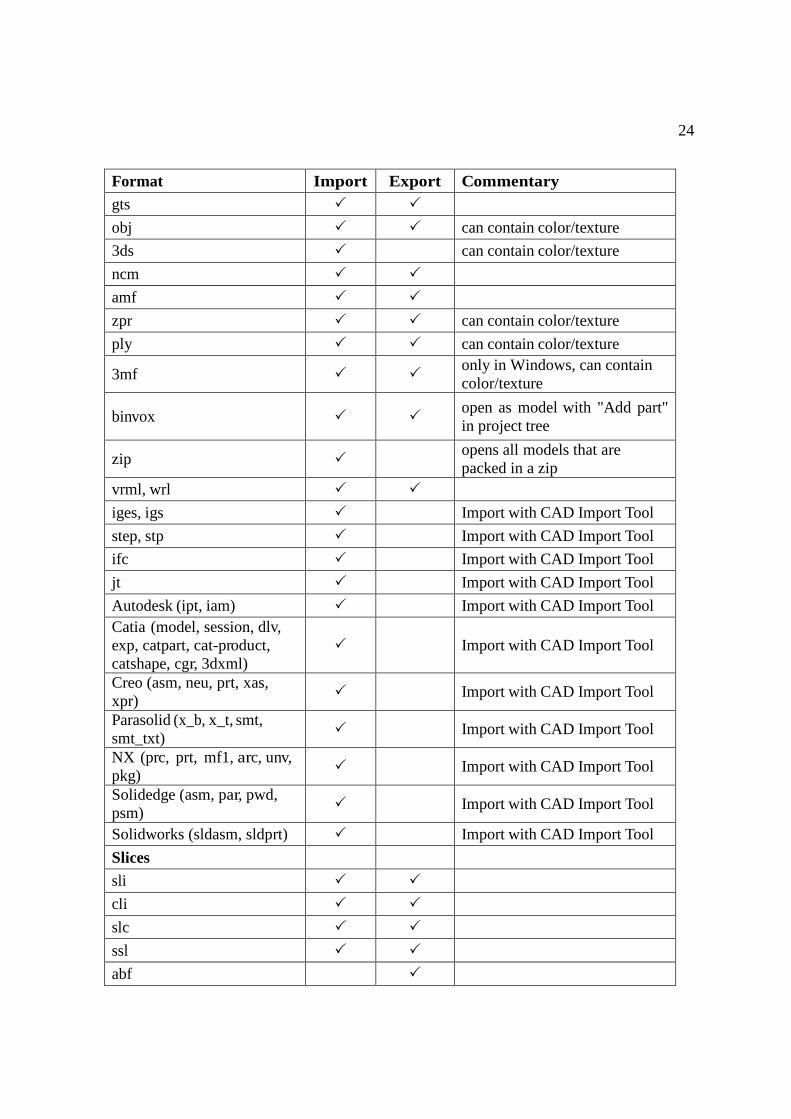
2.5 File Format Overview
In netfabb Professional, there are several file formats available for importing and
exporting parts. With the Professional Tool CAD Import, there are even more possibilities.
Different formats have different qualities, in the following table you’ll get a short overview:
Format Import Export Commentary
netfabb intern
netfabb project � �
3D file formats
STL � �
STL (Ascii) � �
color STL � � can contain color/texture
x3d � � can contain color/texture
x3db � � can contain color/texture
Figure 2.13: Tabsheets of standard interface, repair module and Boolean Operations module
24
Format Import Export Commentary gts � �
obj � � can contain color/texture
3ds � can contain color/texture
ncm � �
amf � �
zpr � � can contain color/texture
ply � � can contain color/texture
3mf � � only in Windows, can contain color/texture
binvox � � open as model with "Add part" in project tree
zip � opens all models that are packed in a zip
vrml, wrl � �
iges, igs � Import with CAD Import Tool
step, stp � Import with CAD Import Tool
ifc � Import with CAD Import Tool
jt � Import with CAD Import Tool
Autodesk (ipt, iam) � Import with CAD Import Tool Catia (model, session, dlv, exp, catpart, cat-product, catshape, cgr, 3dxml)
� Import with CAD Import Tool
Creo (asm, neu, prt, xas, xpr)
� Import with CAD Import Tool
Parasolid (x_b, x_t, smt, smt_txt)
� Import with CAD Import Tool
NX (prc, prt, mf1, arc, unv, pkg)
� Import with CAD Import Tool
Solidedge (asm, par, pwd, psm)
� Import with CAD Import Tool
Solidworks (sldasm, sldprt) � Import with CAD Import Tool
Slices
sli � �
cli � �
slc � �
ssl � �
abf �
25
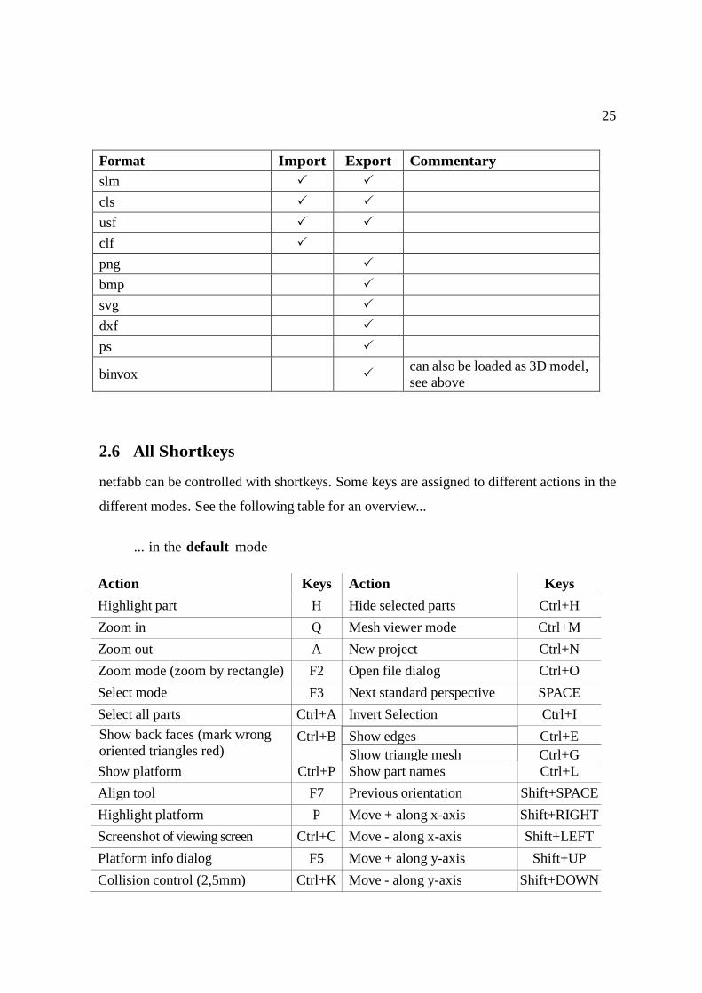
Format Import Export Commentary slm � �
cls � �
usf � �
clf �
png �
bmp �
svg �
dxf �
ps �
binvox � can also be loaded as 3D model, see above
2.6 All Shortkeys
netfabb can be controlled with shortkeys. Some keys are assigned to different actions in the
different modes. See the following table for an overview...
... in the default mode
Action Keys Action Keys
Highlight part H Hide selected parts Ctrl+H
Zoom in Q Mesh viewer mode Ctrl+M
Zoom out A New project Ctrl+N
Zoom mode (zoom by rectangle) F2 Open file dialog Ctrl+O
Select mode F3 Next standard perspective SPACE
Select all parts Ctrl+A Invert Selection Ctrl+I
Show back faces (mark wrong oriented triangles red)
Ctrl+B Show edges Ctrl+E Show triangle mesh Ctrl+G
Show platform Ctrl+P Show part names Ctrl+L
Align tool F7 Previous orientation Shift+SPACE
Highlight platform P Move + along x-axis Shift+RIGHT
Screenshot of viewing screen Ctrl+C Move - along x-axis Shift+LEFT
Platform info dialog F5 Move + along y-axis Shift+UP
Collision control (2,5mm) Ctrl+K Move - along y-axis Shift+DOWN
26
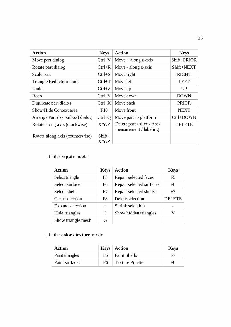
Action Keys Action Keys
Move part dialog Ctrl+V Move + along z-axis Shift+PRIOR
Rotate part dialog Ctrl+R Move - along z-axis Shift+NEXT
Scale part Ctrl+S Move right RIGHT
Triangle Reduction mode Ctrl+T Move left LEFT
Undo Ctrl+Z Move up UP
Redo Ctrl+Y Move down DOWN
Duplicate part dialog Ctrl+X Move back PRIOR
Show/Hide Context area F10 Move front NEXT
Arrange Part (by outbox) dialog Ctrl+Q Move part to platform Ctrl+DOWN
Rotate along axis (clockwise) X/Y/Z Delete part / slice / test / measurement / labeling
DELETE
Rotate along axis (counterwise) Shift+ X/Y/Z
... in the repair mode
Action Keys Action Keys
Select triangle F5 Repair selected faces F5
Select surface F6 Repair selected surfaces F6
Select shell F7 Repair selected shells F7
Clear selection F8 Delete selection DELETE
Expand selection + Shrink selection -
Hide triangles I Show hidden triangles V
Show triangle mesh G
... in the color / texture mode
Action Keys Action Keys
Paint triangles F5 Paint Shells F7
Paint surfaces F6 Texture Pipette F8
27
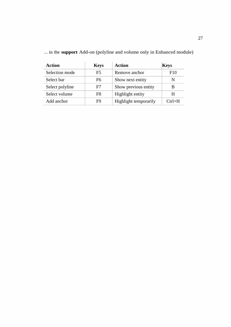
... in the support Add-on (polyline and volume only in Enhanced module)
Action Keys Action Keys
Selection mode F5 Remove anchor F10
Select bar F6 Show next entity N
Select polyline F7 Show previous entity B
Select volume F8 Highlight entity H
Add anchor F9 Highlight temporarily Ctrl+H
28
3 Project Management
There are several methods to manage netfabb projects, read and open files and save or export
projects and parts. To save processing time, STL files with a great complexity can be split
before adding them to a project. For further processing, projects can be saved as netfabb
project files and parts can be exported into three-dimensional or two-and-a-half-
dimensional file formats. Screenshots can be exported and saved for illustration purposes.
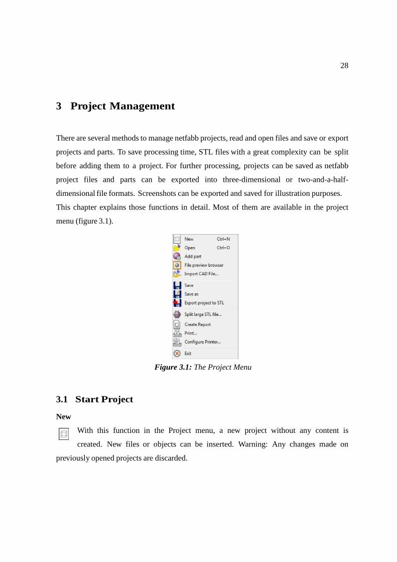
This chapter explains those functions in detail. Most of them are available in the project
menu (figure 3.1).
3.1 Start Project
New
With this function in the Project menu, a new project without any content is
created. New files or objects can be inserted. Warning: Any changes made on
previously opened projects are discarded.
Figure 3.1: The Project Menu
29
Undo/Redo
The Undo function in the Edit menu reverts the last operation on parts in the
default module. Only simple actions such as moving parts or starting new modules
can be undone. If an operation has replaced the original part (such as cutting or a repair), it
cannot be retrieved and the operation cannot be undone. With Redo, you can perform the
process you have undone again.
3.2 Open Files
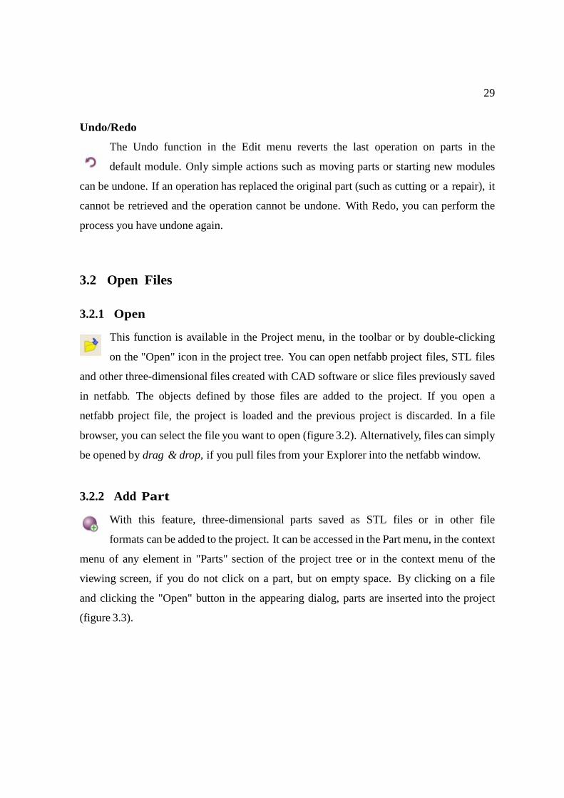
3.2.1 Open
This function is available in the Project menu, in the toolbar or by double-clicking
on the "Open" icon in the project tree. You can open netfabb project files, STL files
and other three-dimensional files created with CAD software or slice files previously saved
in netfabb. The objects defined by those files are added to the project. If you open a
netfabb project file, the project is loaded and the previous project is discarded. In a file
browser, you can select the file you want to open (figure 3.2). Alternatively, files can simply
be opened by drag & drop, if you pull files from your Explorer into the netfabb window.
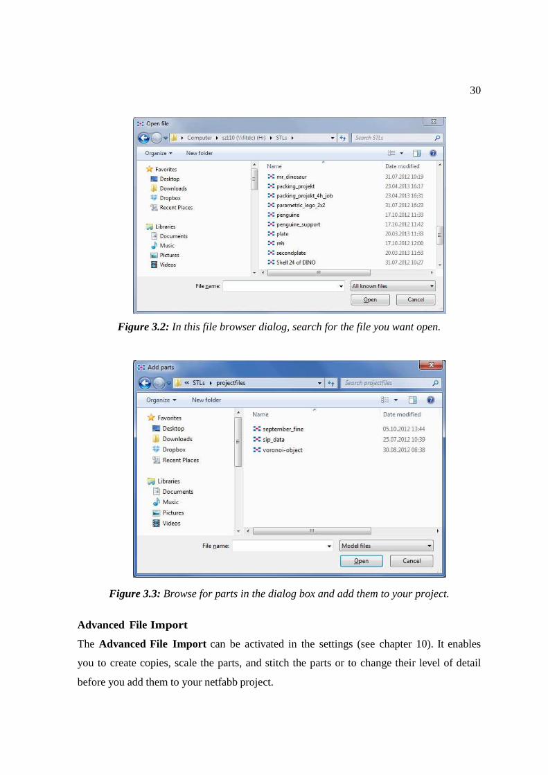
3.2.2 Add Part
With this feature, three-dimensional parts saved as STL files or in other file
formats can be added to the project. It can be accessed in the Part menu, in the context
menu of any element in "Parts" section of the project tree or in the context menu of the
viewing screen, if you do not click on a part, but on empty space. By clicking on a file
and clicking the "Open" button in the appearing dialog, parts are inserted into the project
(figure 3.3).
30
Figure 3.2: In this file browser dialog, search for the file you want open.
Figure 3.3: Browse for parts in the dialog box and add them to your project.
Advanced File Import
The Advanced File Import can be activated in the settings (see chapter 10). It enables
you to create copies, scale the parts, and stitch the parts or to change their level of detail
before you add them to your netfabb project.
31
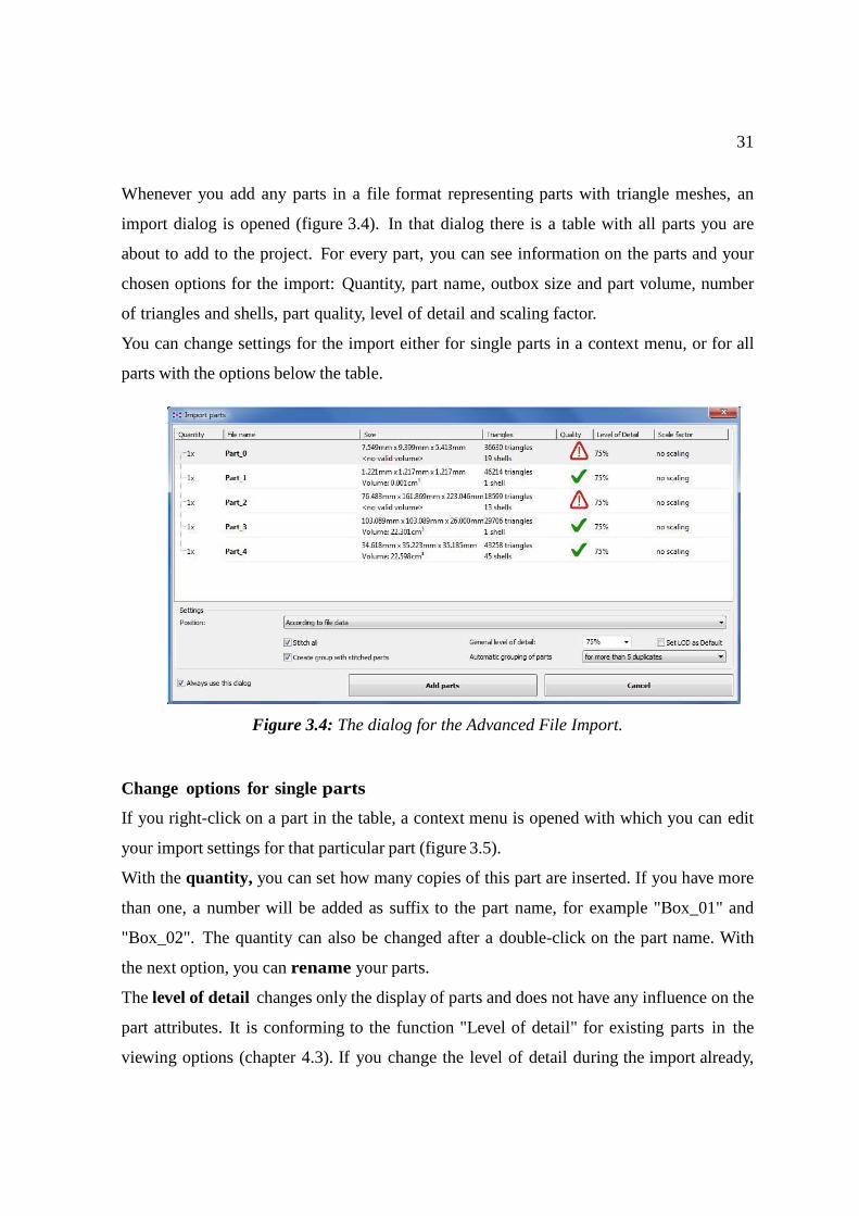
Whenever you add any parts in a file format representing parts with triangle meshes, an
import dialog is opened (figure 3.4). In that dialog there is a table with all parts you are
about to add to the project. For every part, you can see information on the parts and your
chosen options for the import: Quantity, part name, outbox size and part volume, number
of triangles and shells, part quality, level of detail and scaling factor.
You can change settings for the import either for single parts in a context menu, or for all
parts with the options below the table.
Figure 3.4: The dialog for the Advanced File Import.
Change options for single parts
If you right-click on a part in the table, a context menu is opened with which you can edit
your import settings for that particular part (figure 3.5).
With the quantity, you can set how many copies of this part are inserted. If you have more
than one, a number will be added as suffix to the part name, for example "Box_01" and
"Box_02". The quantity can also be changed after a double-click on the part name. With
the next option, you can rename your parts.
The level of detail changes only the display of parts and does not have any influence on the
part attributes. It is conforming to the function "Level of detail" for existing parts in the
viewing options (chapter 4.3). If you change the level of detail during the import already,

32
you can save computing time, as complex parts do not have to be rendered in full detail
from the start.
Figure 3.5: The context menu after a right-click on a part in the import dialog.
To set the scale of parts, you can either perform the functions inches to mm or mm to
inches before opening the parts (see chapter 6.2.3), enter a custom scaling factor or set
back the scaling to the usual part size (100%). You can find these options in a submenu.
If you Stitch, open triangle edges are stitched together immediately, as with the function
"Stitch Triangles" in the repair module (chapter 7.5.3). This may or may not repair the
part, but will almost always improve the part quality. When triangle edges are stitched,
you can see instant changes in the number of triangles and shells and in the part quality. If
parts are damaged, there is a warning sign in the column for the part quality (the same as
for damaged parts in the project). If they are good, there is a green check.
If you click on Remove in the context menu, the part will no longer appear on the list and
will not be added to the project.
Settings for all parts
Below the list of parts, you can edit settings which apply for all parts. For the positioning
of the parts, you can choose one of three options in a dropdown menu:
• According to file data: All parts are positioned exactly as defined in the file. Most
three-dimensional files contain positional information.
• Move parts to origin: All parts are moved to the origin. The lowest outbox
coordinates will be X=0, Y=0, Z=0
• Arrange parts: All parts are arranged next together in the platform, with their
outbox as reference. The first part is inserted at the origin.
33
If the box Stitch all is ticked, the triangles of every part are stitched when you add the
parts.
The General level of detail sets the level of detail for all parts. Choose a value in the
dropdown menu. If you tick the box Set LOD (level of detail) as default, your level of
detail value will become standard for the Advanced File Import.
The option Move stitched parts into group generates a group in your project into which
all added parts which have been stitched are moved. Parts that are not damaged or cannot be
stitched at all, but are stitched nevertheless (for example with the option "Stitch all") are not
moved into this group.
In the bottom left there is the option Always use this dialog. If you deactivate this, the
advanced file import will no longer appear when you add parts. You can reactivate it in the
settings.
If you increase the quantity of the single parts to more than 5, you can let the parts be
organized in groups. For example, you open a part and want to load it 12 times, change
the Automatic grouping of parts to more than 10 duplicates. All 12 parts will then be
organized in 1 group in the project tree.
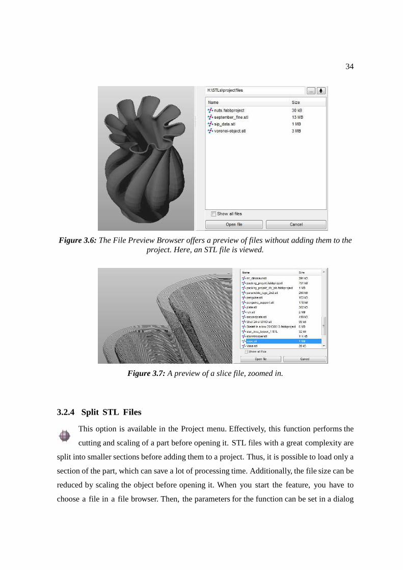
3.2.3 File Preview Browser
The File Preview Browser is available in the Project menu and opens a browser
window in the tabsheet, where it is possible to search for and open files. If you
click on a file name, a preview of the object is displayed on the viewing screen without it
being added to your project. You can also scroll through files with your cursor buttons.
The preview can be obtained for both three-dimensional files and two-and-a-half-
dimensional slice files with various file formats. Clicking on "Open" or double-clicking
on the file name inserts the selected file into your project. That way, the file preview
browser allows a quick browsing of databases without necessarily opening each part to
look at it (figure 3.6, 3.7). Viewing options such as zooming in and changing perspectives
are available as in an open project.
34
Figure 3.6: The File Preview Browser offers a preview of files without adding them to the project. Here, an STL file is viewed.
Figure 3.7: A preview of a slice file, zoomed in.
3.2.4 Split STL Files
This option is available in the Project menu. Effectively, this function performs the
cutting and scaling of a part before opening it. STL files with a great complexity are
split into smaller sections before adding them to a project. Thus, it is possible to load only a
section of the part, which can save a lot of processing time. Additionally, the file size can be
reduced by scaling the object before opening it. When you start the feature, you have to
choose a file in a file browser. Then, the parameters for the function can be set in a dialog
35
box. The STL Information specifies the size of the outbox of the part, the number of
triangles and the size of the STL file. The outbox is a cuboid space enclosing the part.
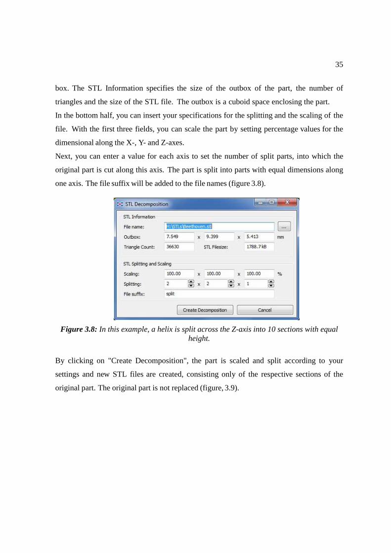
In the bottom half, you can insert your specifications for the splitting and the scaling of the
file. With the first three fields, you can scale the part by setting percentage values for the
dimensional along the X-, Y- and Z-axes.
Next, you can enter a value for each axis to set the number of split parts, into which the
original part is cut along this axis. The part is split into parts with equal dimensions along
one axis. The file suffix will be added to the file names (figure 3.8).
Figure 3.8: In this example, a helix is split across the Z-axis into 10 sections with equal height.
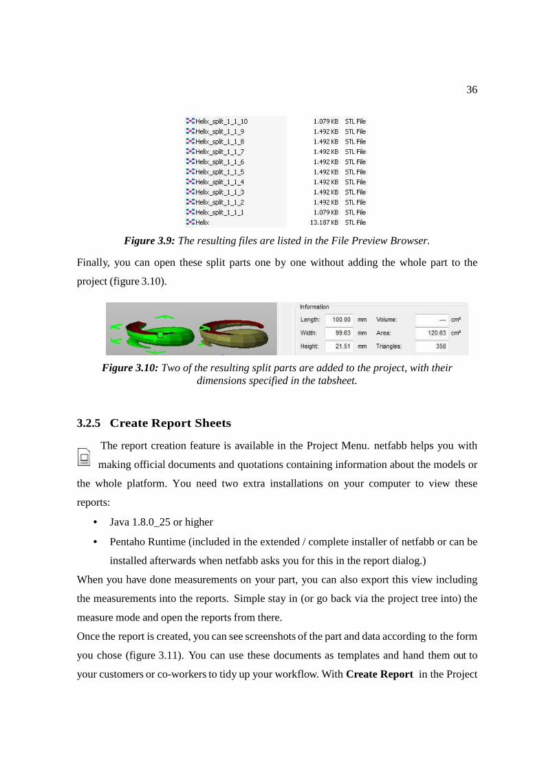
By clicking on "Create Decomposition", the part is scaled and split according to your
settings and new STL files are created, consisting only of the respective sections of the
original part. The original part is not replaced (figure, 3.9).
36
Figure 3.9: The resulting files are listed in the File Preview Browser.
Finally, you can open these split parts one by one without adding the whole part to the
project (figure 3.10).
Figure 3.10: Two of the resulting split parts are added to the project, with their dimensions specified in the tabsheet.
3.2.5 Create Report Sheets
The report creation feature is available in the Project Menu. netfabb helps you with
making official documents and quotations containing information about the models or
the whole platform. You need two extra installations on your computer to view these
reports:
• Java 1.8.0_25 or higher
• Pentaho Runtime (included in the extended / complete installer of netfabb or can be
installed afterwards when netfabb asks you for this in the report dialog.)
When you have done measurements on your part, you can also export this view including
the measurements into the reports. Simple stay in (or go back via the project tree into) the
measure mode and open the reports from there.
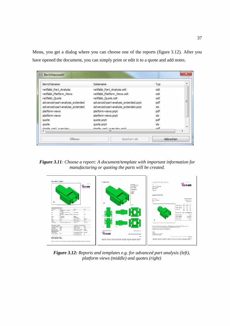
Once the report is created, you can see screenshots of the part and data according to the form
you chose (figure 3.11). You can use these documents as templates and hand them out to
your customers or co-workers to tidy up your workflow. With Create Report in the Project
37
Menu, you get a dialog where you can choose one of the reports (figure 3.12). After you
have opened the document, you can simply print or edit it to a quote and add notes.
Figure 3.11: Choose a report: A document/template with important information for manufacturing or quoting the parts will be created.
Figure 3.12: Reports and templates e.g. for advanced part analysis (left), platform views (middle) and quotes (right)
38
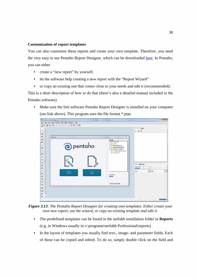
Customization of report templates
You can also customize these reports and create your own template. Therefore, you need
the very easy to use Pentaho Report Designer, which can be downloaded here. In Pentaho,
you can either
• create a “new report” by yourself,
• let the software help creating a new report with the “Report Wizard”
• or copy an existing one that comes close to your needs and edit it (recommended):
This is a short description of how to do that (there’s also a detailed manual included in the
Pentaho software).
• Make sure the free software Pentaho Report Designer is installed on your computer
(see link above). This program uses the file format *.prpt.
Figure 3.13: The Pentaho Report Designer for creating own templates. Either create your own new report, use the wizard, or copy an existing template and edit it.
• The predefined templates can be found in the netfabb installation folder in Reports
(e.g. in Windows usually in c:\programs\netfabb Professional\reports)
• In the layout of templates you usually find text-, image- and parameter fields. Each
of those can be copied and edited. To do so, simply double click on the field and
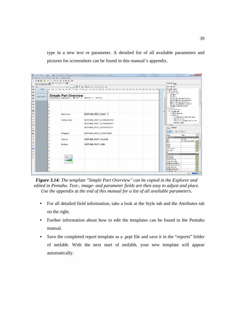
39
type in a new text or parameter. A detailed list of all available parameters and
pictures for screenshots can be found in this manual’s appendix.
• For all detailed field information, take a look at the Style tab and the Attributes tab
on the right.
• Further information about how to edit the templates can be found in the Pentaho
manual.
• Save the completed report template as a .prpt file and save it in the “reports” folder
of netfabb. With the next start of netfabb, your new template will appear
automatically.
Figure 3.14: The template "Simple Part Overview" can be copied in the Explorer and edited in Pentaho. Text-, image- and parameter fields are then easy to adjust and place.
Use the appendix at the end of this manual for a list of all available parameters.
40
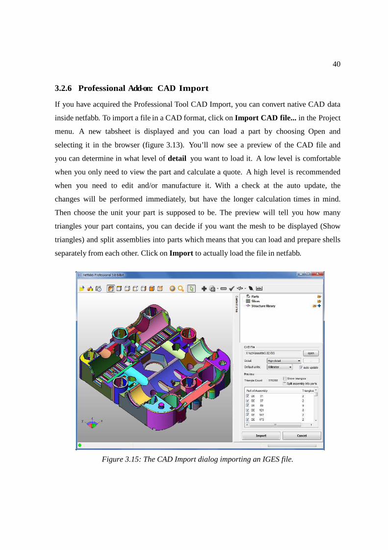
3.2.6 Professional Add-on: CAD Import
If you have acquired the Professional Tool CAD Import, you can convert native CAD data
inside netfabb. To import a file in a CAD format, click on Import CAD file... in the Project
menu. A new tabsheet is displayed and you can load a part by choosing Open and
selecting it in the browser (figure 3.13). You’ll now see a preview of the CAD file and
you can determine in what level of detail you want to load it. A low level is comfortable
when you only need to view the part and calculate a quote. A high level is recommended
when you need to edit and/or manufacture it. With a check at the auto update, the
changes will be performed immediately, but have the longer calculation times in mind.
Then choose the unit your part is supposed to be. The preview will tell you how many
triangles your part contains, you can decide if you want the mesh to be displayed (Show
triangles) and split assemblies into parts which means that you can load and prepare shells
separately from each other. Click on Import to actually load the file in netfabb.
Figure 3.15: The CAD Import dialog importing an IGES file.

41
3.3 Save and Export
3.3.1 Save
If you choose Save in the Project menu, the project is saved and its previously saved
version is overwritten.
If you choose Save As or if there is no existing version of the project, a dialog
window is opened, in which target directory, file name and file type can be chosen
(figure 3.14).
Figure 3.16: Choose target directory and file type and insert file name in the browser dialog.
3.3.2 Export Project to STL
The entire project, possibly consisting of many different parts, is saved as one single
STL file. Target directory and file name can be chosen in a file browser.
42
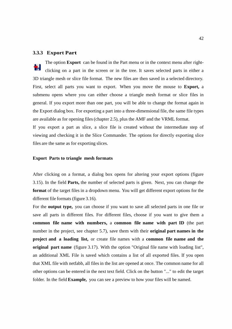
3.3.3 Export Part
The option Export can be found in the Part menu or in the context menu after right-
clicking on a part in the screen or in the tree. It saves selected parts in either a
3D triangle mesh or slice file format. The new files are then saved in a selected directory.
First, select all parts you want to export. When you move the mouse to Export, a
submenu opens where you can either choose a triangle mesh format or slice files in
general. If you export more than one part, you will be able to change the format again in
the Export dialog box. For exporting a part into a three-dimensional file, the same file types
are available as for opening files (chapter 2.5), plus the AMF and the VRML format.
If you export a part as slice, a slice file is created without the intermediate step of
viewing and checking it in the Slice Commander. The options for directly exporting slice
files are the same as for exporting slices. Export Parts to triangle mesh formats
After clicking on a format, a dialog box opens for altering your export options (figure
3.15). In the field Parts, the number of selected parts is given. Next, you can change the
format of the target files in a dropdown menu. You will get different export options for the
different file formats (figure 3.16).
For the output type, you can choose if you want to save all selected parts in one file or
save all parts in different files. For different files, choose if you want to give them a
common file name with numbers, a common file name with part ID (the part
number in the project, see chapter 5.7), save them with their original part names in the
project and a loading list, or create file names with a common file name and the
original part name (figure 3.17). With the option "Original file name with loading list",
an additional XML File is saved which contains a list of all exported files. If you open
that XML file with netfabb, all files in the list are opened at once. The common name for all
other options can be entered in the next text field. Click on the button "..." to edit the target
folder. In the field Example, you can see a preview to how your files will be named.
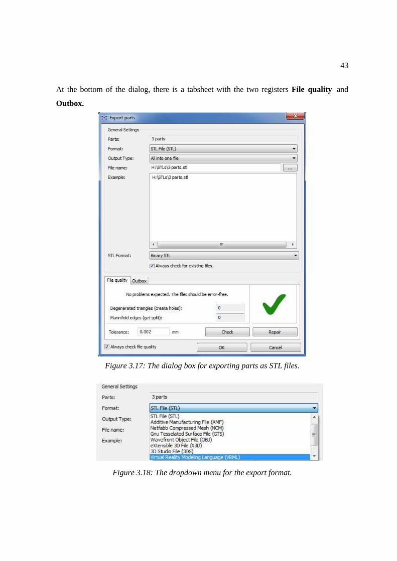
43
At the bottom of the dialog, there is a tabsheet with the two registers File quality and
Outbox.
Figure 3.17: The dialog box for exporting parts as STL files.
Figure 3.18: The dropdown menu for the export format.
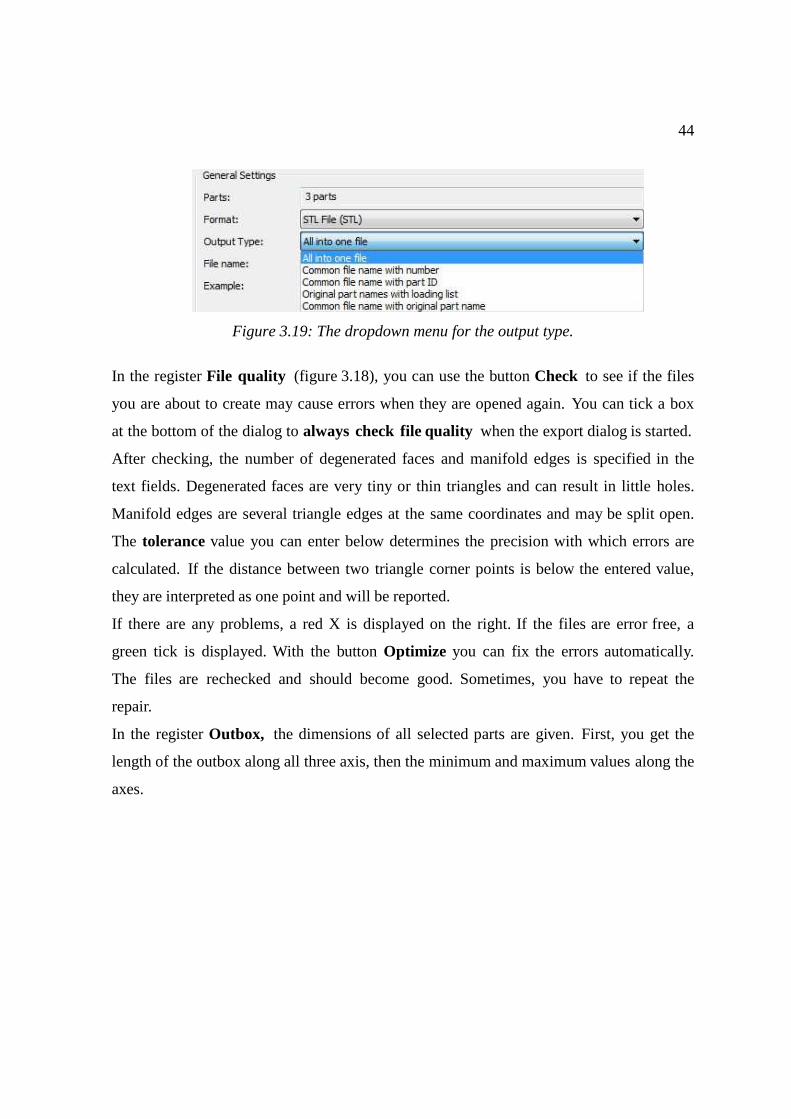
44
Figure 3.19: The dropdown menu for the output type.
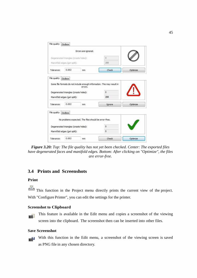
In the register File quality (figure 3.18), you can use the button Check to see if the files
you are about to create may cause errors when they are opened again. You can tick a box
at the bottom of the dialog to always check file quality when the export dialog is started.
After checking, the number of degenerated faces and manifold edges is specified in the
text fields. Degenerated faces are very tiny or thin triangles and can result in little holes.
Manifold edges are several triangle edges at the same coordinates and may be split open.
The tolerance value you can enter below determines the precision with which errors are
calculated. If the distance between two triangle corner points is below the entered value,
they are interpreted as one point and will be reported.
If there are any problems, a red X is displayed on the right. If the files are error free, a
green tick is displayed. With the button Optimize you can fix the errors automatically.
The files are rechecked and should become good. Sometimes, you have to repeat the
repair.
In the register Outbox, the dimensions of all selected parts are given. First, you get the
length of the outbox along all three axis, then the minimum and maximum values along the
axes.
45
Figure 3.20: Top: The file quality has not yet been checked. Center: The exported files have degenerated faces and manifold edges. Bottom: After clicking on "Optimize", the files
are error-free.
3.4 Prints and Screenshots
This function in the Project menu directly prints the current view of the project.
With "Configure Printer", you can edit the settings for the printer.
Screenshot to Clipboard
This feature is available in the Edit menu and copies a screenshot of the viewing
screen into the clipboard. The screenshot then can be inserted into other files.
Save Screenshot
With this function in the Edit menu, a screenshot of the viewing screen is saved
as PNG file in any chosen directory.
46
4 Viewing Options
The view to a project in the viewing screen can be altered in many ways. The perspective
from which objects are seen can be set to seven different standard directions or can be
intuitively rotated by use of the mouse. To shift the view on the displayed project or to
zoom in and out, you can also use the mouse very easily, or use one of several standard
zoom options.
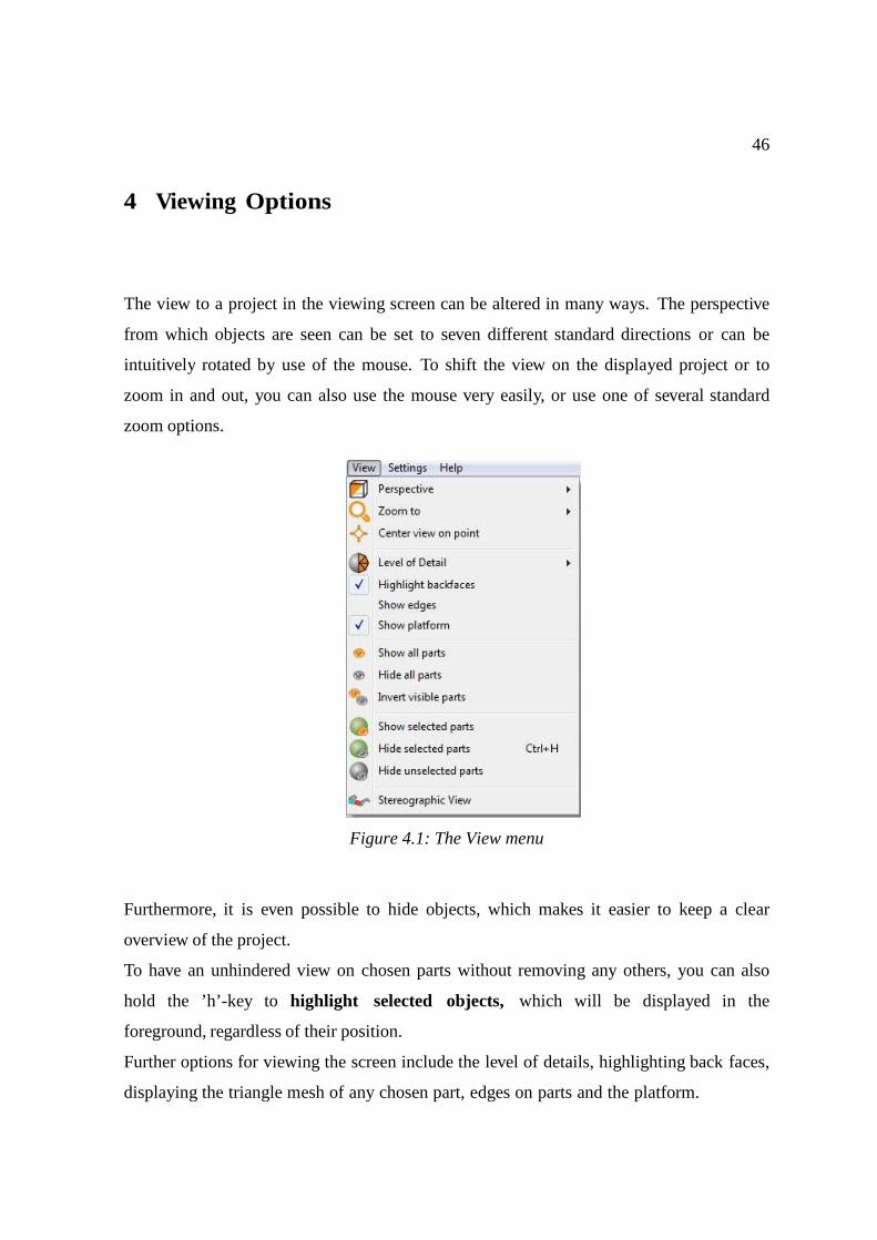
Figure 4.1: The View menu
Furthermore, it is even possible to hide objects, which makes it easier to keep a clear
overview of the project.
To have an unhindered view on chosen parts without removing any others, you can also
hold the ’h’-key to highlight selected objects, which will be displayed in the
foreground, regardless of their position.
Further options for viewing the screen include the level of details, highlighting back faces,
displaying the triangle mesh of any chosen part, edges on parts and the platform.

47
4.1 Perspectives
The perspective refers to the direction from which a project is viewed. In the bottom
left of the viewing screen is a coordinate system indicating the current viewing
perspective (figure 4.2).
Figure 4.2: Three Different Perspectives with the Coordinate System
To change the perspective, there are two ways. First, by holding the right mouse button
and moving the mouse in the direction you want to turn the project visually, the
perspective can be intuitively rotated to any position, with the center of the screen as center
of rotation. If you right-click close to the edge of the screen, the perspective is only changed
two-dimensionally to the left, right, up and down.
If you want a certain point on a part as center of rotation, right-click on this point and
click on "Center View Here" in the context menu. Your view will be shifted and the point
you clicked on moved into the center, subsequently becoming the center of rotation.
Second, there are seven standard perspectives. The perspectives from the top, bottom,
left, right, front and back refer to the coordinate system, whereas the front is the X-Z-
plane. The isometric view is a view from the front-left-top-corner of the platform. That
way, you gain a kind of three-dimensional view on the project and on objects which are
aligned along the axes (figure 4.3).
48
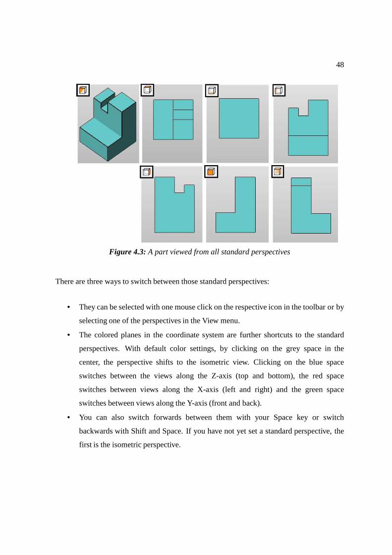
Figure 4.3: A part viewed from all standard perspectives
There are three ways to switch between those standard perspectives:
• They can be selected with one mouse click on the respective icon in the toolbar or by
selecting one of the perspectives in the View menu.
• The colored planes in the coordinate system are further shortcuts to the standard
perspectives. With default color settings, by clicking on the grey space in the
center, the perspective shifts to the isometric view. Clicking on the blue space
switches between the views along the Z-axis (top and bottom), the red space
switches between views along the X-axis (left and right) and the green space
switches between views along the Y-axis (front and back).
• You can also switch forwards between them with your Space key or switch
backwards with Shift and Space. If you have not yet set a standard perspective, the
first is the isometric perspective.
49
4.2 Centering and Zooming
Shift View
By holding the central mouse button and moving the mouse, the view on a project can be
shifted to the right, left, up or down. This changes only the center of the main screen
without changing the perspective. If you do not have a central mouse button, hold Shift and
use the right mouse button.
Center View
When you right-click on a part in the screen, the option Center View Here is
available in the context menu to shift the view. The point you clicked on is then
moved into the center of the viewing screen. The option is also available in the View
menu. After selecting the option there, left-click on the point you want to move into the
center.
Zoom
The scroll button of the mouse can be used to zoom in and out. If you roll forward, you
zoom in and if you roll backwards, you zoom out. If you do not have a scroll button, hold
both Ctrl and the right mouse button and move the mouse up and down. With the keyboard,
you can zoom in with Q and zoom out with A.
Additionally, there are several default options to center and zoom. Depending on which
function you choose, netfabb moves certain components into the center and resets the
zoom so that these components fit exactly into the screen. These options are available by
clicking on the respective icons in the toolbar or in the View menu.
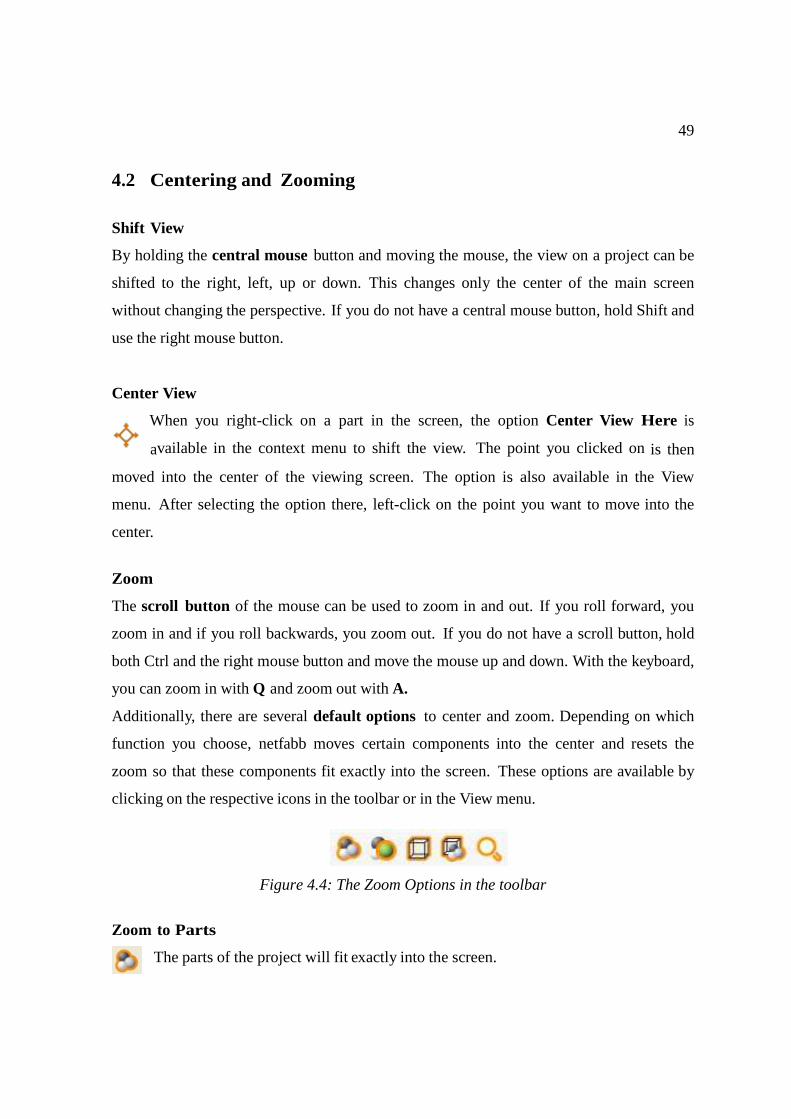
Figure 4.4: The Zoom Options in the toolbar
Zoom to Parts
The parts of the project will fit exactly into the screen.
50
Zoom to Selected Parts
The screen will include all selected parts.
Zoom to Platform
netfabb calculates a frame for the viewing screen which contains the platform.
Zoom to All
The View will include all parts and the whole platform.
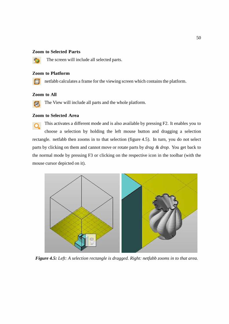
Zoom to Selected Area
This activates a different mode and is also available by pressing F2. It enables you to
choose a selection by holding the left mouse button and dragging a selection
rectangle. netfabb then zooms in to that selection (figure 4.5). In turn, you do not select
parts by clicking on them and cannot move or rotate parts by drag & drop. You get back to
the normal mode by pressing F3 or clicking on the respective icon in the toolbar (with the
mouse cursor depicted on it).
Figure 4.5: Left: A selection rectangle is dragged. Right: netfabb zooms in to that area.
51
4.3 Displaying Options
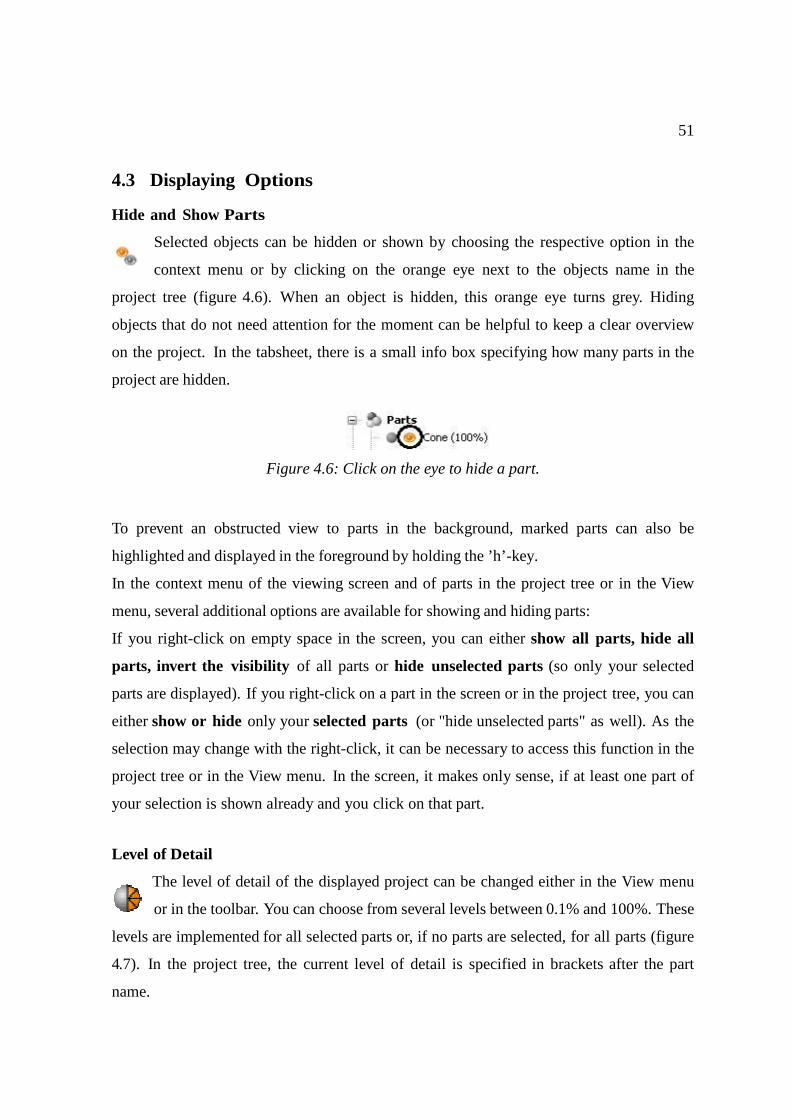
Hide and Show Parts
Selected objects can be hidden or shown by choosing the respective option in the
context menu or by clicking on the orange eye next to the objects name in the
project tree (figure 4.6). When an object is hidden, this orange eye turns grey. Hiding
objects that do not need attention for the moment can be helpful to keep a clear overview
on the project. In the tabsheet, there is a small info box specifying how many parts in the
project are hidden.
Figure 4.6: Click on the eye to hide a part.
To prevent an obstructed view to parts in the background, marked parts can also be
highlighted and displayed in the foreground by holding the ’h’-key.
In the context menu of the viewing screen and of parts in the project tree or in the View
menu, several additional options are available for showing and hiding parts:
If you right-click on empty space in the screen, you can either show all parts, hide all
parts, invert the visibility of all parts or hide unselected parts (so only your selected
parts are displayed). If you right-click on a part in the screen or in the project tree, you can
either show or hide only your selected parts (or "hide unselected parts" as well). As the
selection may change with the right-click, it can be necessary to access this function in the
project tree or in the View menu. In the screen, it makes only sense, if at least one part of
your selection is shown already and you click on that part. Level of Detail
The level of detail of the displayed project can be changed either in the View menu
or in the toolbar. You can choose from several levels between 0.1% and 100%. These
levels are implemented for all selected parts or, if no parts are selected, for all parts (figure
4.7). In the project tree, the current level of detail is specified in brackets after the part
name.
52
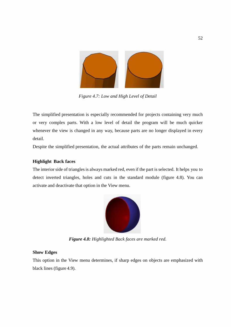
Figure 4.7: Low and High Level of Detail
The simplified presentation is especially recommended for projects containing very much
or very complex parts. With a low level of detail the program will be much quicker
whenever the view is changed in any way, because parts are no longer displayed in every
detail.
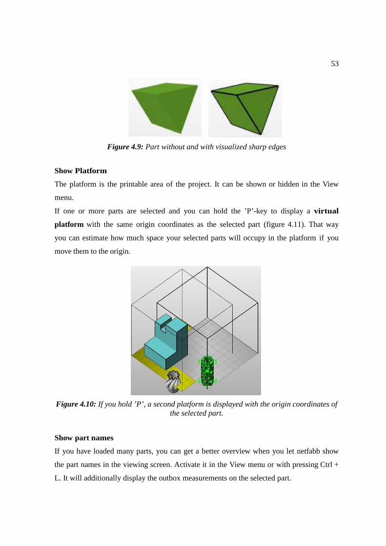
Despite the simplified presentation, the actual attributes of the parts remain unchanged. Highlight Back faces
The interior side of triangles is always marked red, even if the part is selected. It helps you to
detect inverted triangles, holes and cuts in the standard module (figure 4.8). You can
activate and deactivate that option in the View menu.
Figure 4.8: Highlighted Back faces are marked red.
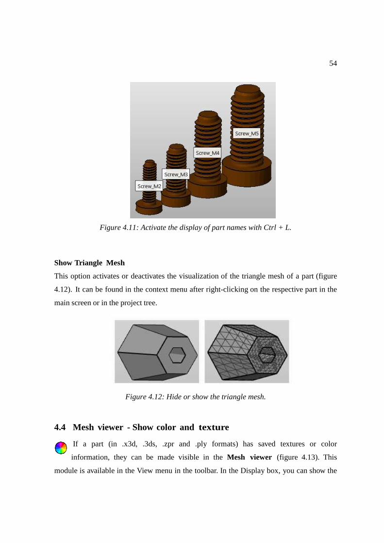
Show Edges
This option in the View menu determines, if sharp edges on objects are emphasized with
black lines (figure 4.9).
53
Figure 4.9: Part without and with visualized sharp edges
Show Platform
The platform is the printable area of the project. It can be shown or hidden in the View
menu.
If one or more parts are selected and you can hold the ’P’-key to display a virtual
platform with the same origin coordinates as the selected part (figure 4.11). That way
you can estimate how much space your selected parts will occupy in the platform if you
move them to the origin.
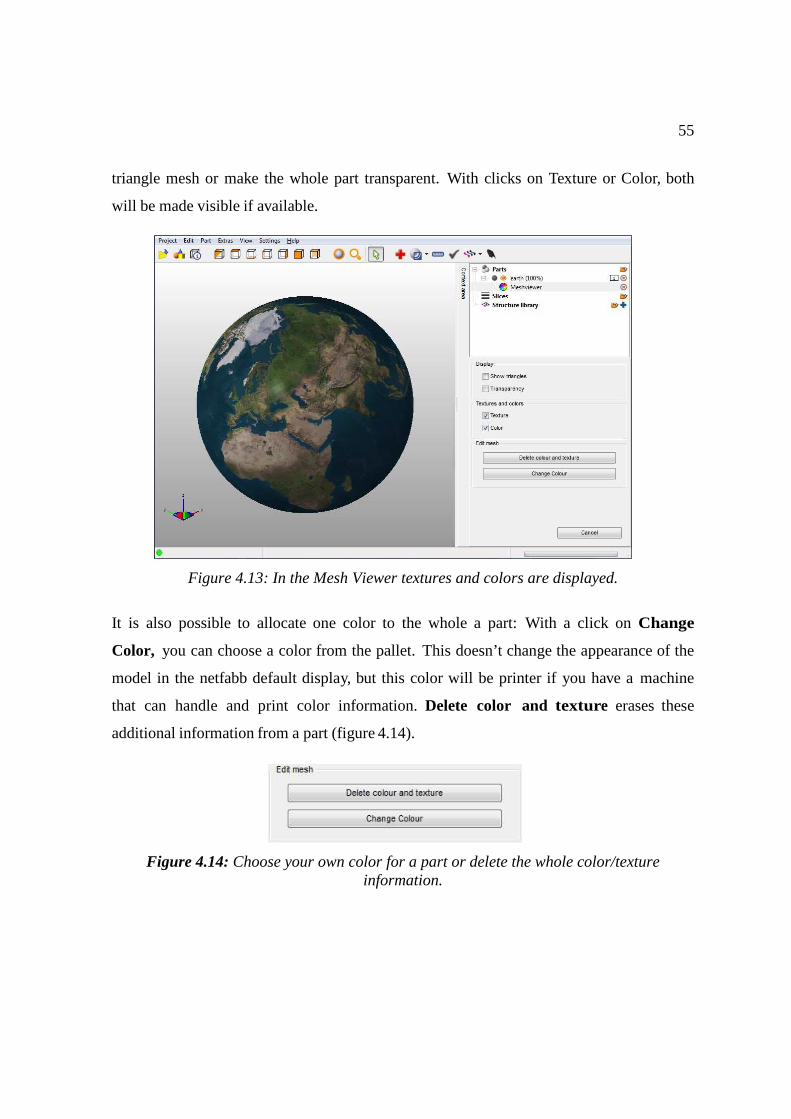
Figure 4.10: If you hold ’P’, a second platform is displayed with the origin coordinates of the selected part.
Show part names
If you have loaded many parts, you can get a better overview when you let netfabb show
the part names in the viewing screen. Activate it in the View menu or with pressing Ctrl +
L. It will additionally display the outbox measurements on the selected part.
54
Figure 4.11: Activate the display of part names with Ctrl + L.
Show Triangle Mesh
This option activates or deactivates the visualization of the triangle mesh of a part (figure
4.12). It can be found in the context menu after right-clicking on the respective part in the
main screen or in the project tree.
Figure 4.12: Hide or show the triangle mesh.
4.4 Mesh viewer - Show color and texture
If a part (in .x3d, .3ds, .zpr and .ply formats) has saved textures or color
information, they can be made visible in the Mesh viewer (figure 4.13). This
module is available in the View menu in the toolbar. In the Display box, you can show the
55
triangle mesh or make the whole part transparent. With clicks on Texture or Color, both
will be made visible if available.
Figure 4.13: In the Mesh Viewer textures and colors are displayed.
It is also possible to allocate one color to the whole a part: With a click on Change
Color, you can choose a color from the pallet. This doesn’t change the appearance of the
model in the netfabb default display, but this color will be printer if you have a machine
that can handle and print color information. Delete color and texture erases these
additional information from a part (figure 4.14).
Figure 4.14: Choose your own color for a part or delete the whole color/texture information.
56
5 Part Management
The part management for netfabb includes the creation of primitive parts, the
duplication of parts, part attributes, positioning and scaling, a platform overview and
collision detection. For managing and editing parts, they must be selected first.
5.1 Add and Remove Parts
Saved parts can be added to the project either with the function Add Part
(chapter 3.2.2) or with the File Preview Browser (chapter 3.2.3). You can also
add parts by drag & drop, if you pull them from your windows folder into your netfabb
window.
A selected part in the project can also be removed and deleted from the current
project. This function can be accessed via the Part menu, in the context menu after
right-clicking on the part to be removed, by double-clicking on the red X-icon next to the
part in the project tree or by pressing the Delete key on the keyboard after selecting the part.
5.2 Select Parts
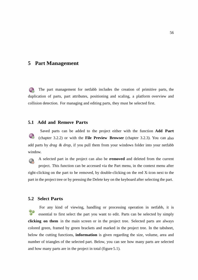
For any kind of viewing, handling or processing operation in netfabb, it is
essential to first select the part you want to edit. Parts can be selected by simply
clicking on them in the main screen or in the project tree. Selected parts are always
colored green, framed by green brackets and marked in the project tree. In the tabsheet,
below the cutting functions, information is given regarding the size, volume, area and
number of triangles of the selected part. Below, you can see how many parts are selected
and how many parts are in the project in total (figure 5.1).
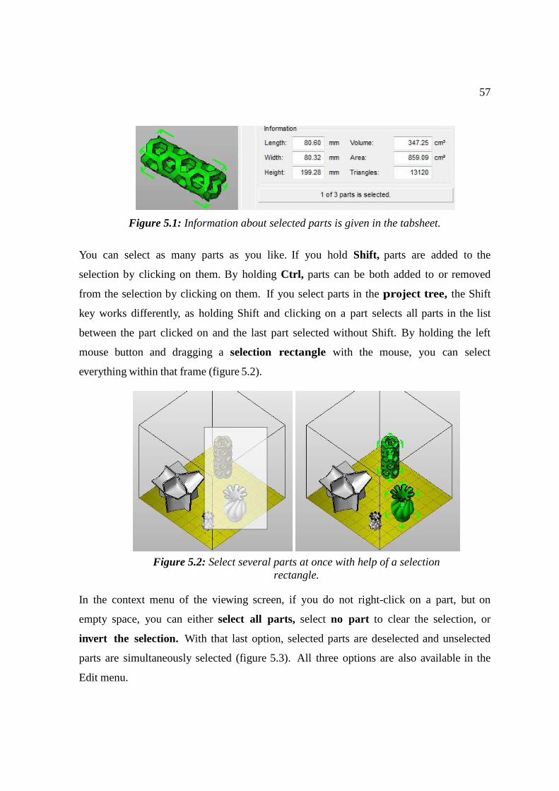
57
Figure 5.1: Information about selected parts is given in the tabsheet.
You can select as many parts as you like. If you hold Shift, parts are added to the
selection by clicking on them. By holding Ctrl, parts can be both added to or removed
from the selection by clicking on them. If you select parts in the project tree, the Shift
key works differently, as holding Shift and clicking on a part selects all parts in the list
between the part clicked on and the last part selected without Shift. By holding the left
mouse button and dragging a selection rectangle with the mouse, you can select
everything within that frame (figure 5.2).
In the context menu of the viewing screen, if you do not right-click on a part, but on
empty space, you can either select all parts, select no part to clear the selection, or
invert the selection. With that last option, selected parts are deselected and unselected
parts are simultaneously selected (figure 5.3). All three options are also available in the
Edit menu.
Figure 5.2: Select several parts at once with help of a selection rectangle.
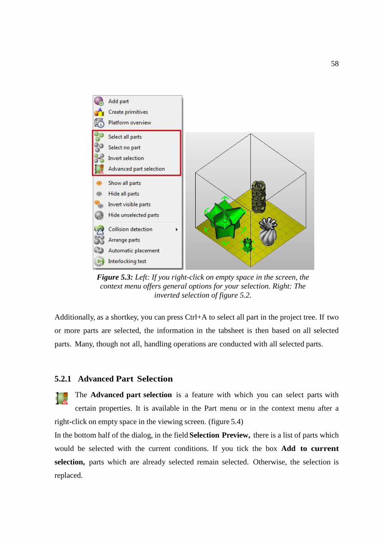
58
Additionally, as a shortkey, you can press Ctrl+A to select all part in the project tree. If two
or more parts are selected, the information in the tabsheet is then based on all selected
parts. Many, though not all, handling operations are conducted with all selected parts.
5.2.1 Advanced Part Selection
The Advanced part selection is a feature with which you can select parts with
certain properties. It is available in the Part menu or in the context menu after a
right-click on empty space in the viewing screen. (figure 5.4)
In the bottom half of the dialog, in the field Selection Preview, there is a list of parts which
would be selected with the current conditions. If you tick the box Add to current
selection, parts which are already selected remain selected. Otherwise, the selection is
replaced.
Figure 5.3: Left: If you right-click on empty space in the screen, the context menu offers general options for your selection. Right: The
inverted selection of figure 5.2.
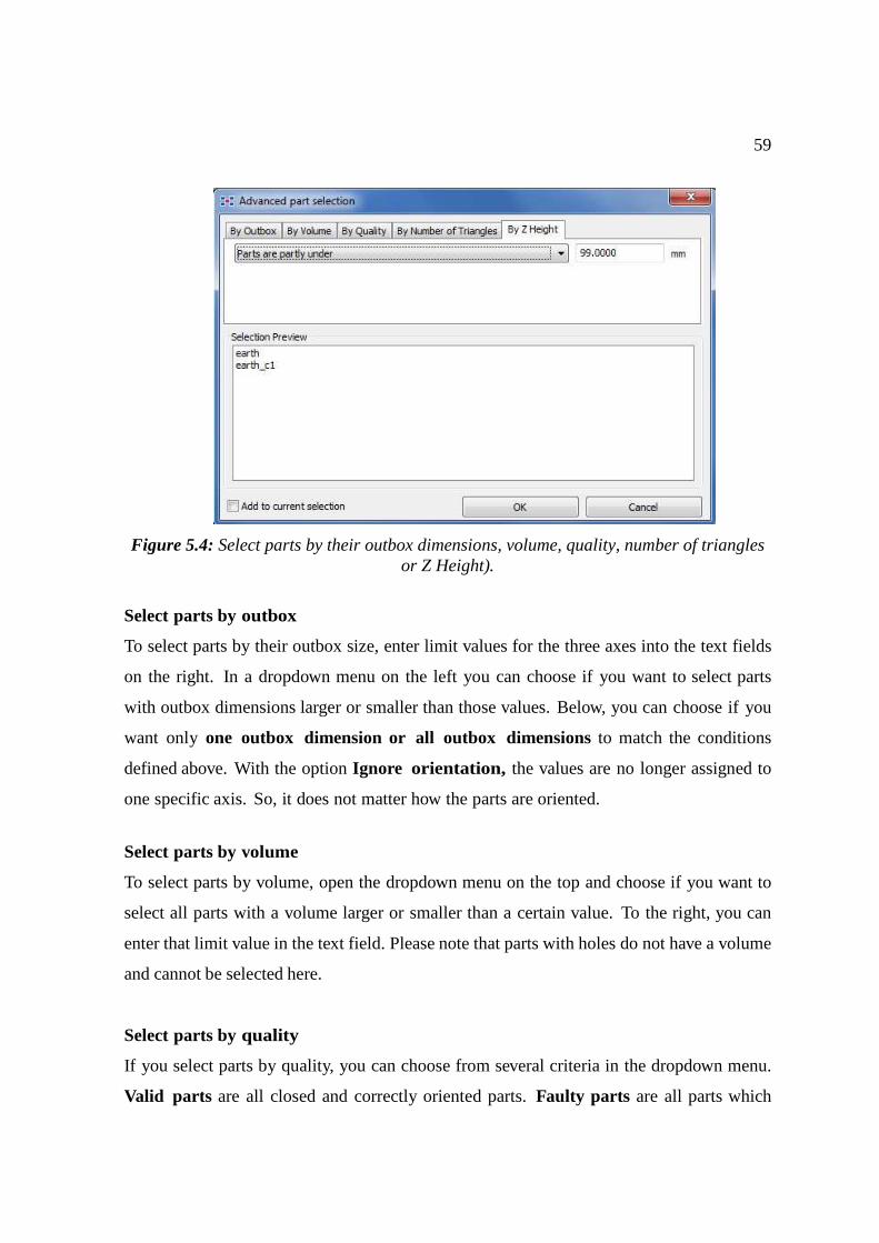
59
Figure 5.4: Select parts by their outbox dimensions, volume, quality, number of triangles or Z Height).
Select parts by outbox
To select parts by their outbox size, enter limit values for the three axes into the text fields
on the right. In a dropdown menu on the left you can choose if you want to select parts
with outbox dimensions larger or smaller than those values. Below, you can choose if you
want only one outbox dimension or all outbox dimensions to match the conditions
defined above. With the option Ignore orientation, the values are no longer assigned to
one specific axis. So, it does not matter how the parts are oriented.
Select parts by volume
To select parts by volume, open the dropdown menu on the top and choose if you want to
select all parts with a volume larger or smaller than a certain value. To the right, you can
enter that limit value in the text field. Please note that parts with holes do not have a volume
and cannot be selected here.
Select parts by quality
If you select parts by quality, you can choose from several criteria in the dropdown menu.
Valid parts are all closed and correctly oriented parts. Faulty parts are all parts which
60
are not valid. Closed parts are all parts without any open triangle edges or holes. The
orientation is ignored. Parts with holes do have open edges. Oriented parts, unlike
non-oriented parts, are parts where all triangles are oriented correctly, with the outside of
a triangle on the outside of the part. Further options are Parts with more than one shell,
Parts with exactly one shell and Parts without triangles.
Select parts by their number of triangles
To select parts by their number of triangles, open the dropdown menu on the top and choose
if you want to select all parts with more or all parts with less than a certain number of
triangles. To the right, you can enter that number of triangles.
Select parts by their Z Height
You can select parts by their Z Height which can be quite practical for packing a build
volume. Choose if the parts are supposed to be completely over or under a certain value or
if they partially can be smaller or bigger.
5.3 Standard models - the part library
Standard models are simple three-dimensional objects that are can be created with a
few clicks in netfabb. After clicking on the Part library icon in the toolbar or
choosing the respective option in the Edit menu, the user can choose from a list of simple
three-dimensional objects that can be selected with a double-click and inserted into the
project (figure 5.5). Although their basic geometry is already given, there are many
parameters that can be specified in detail by the user.
That way, you can create a variety of parts. The settings can be saved as default setting for
the primitive part by clicking on the button below. The button "Load Default" restores the
default settings after the parameters have been changed. By clicking on Apply, the part is
inserted into the project. In the following list, you can find a short description of each
parameter:
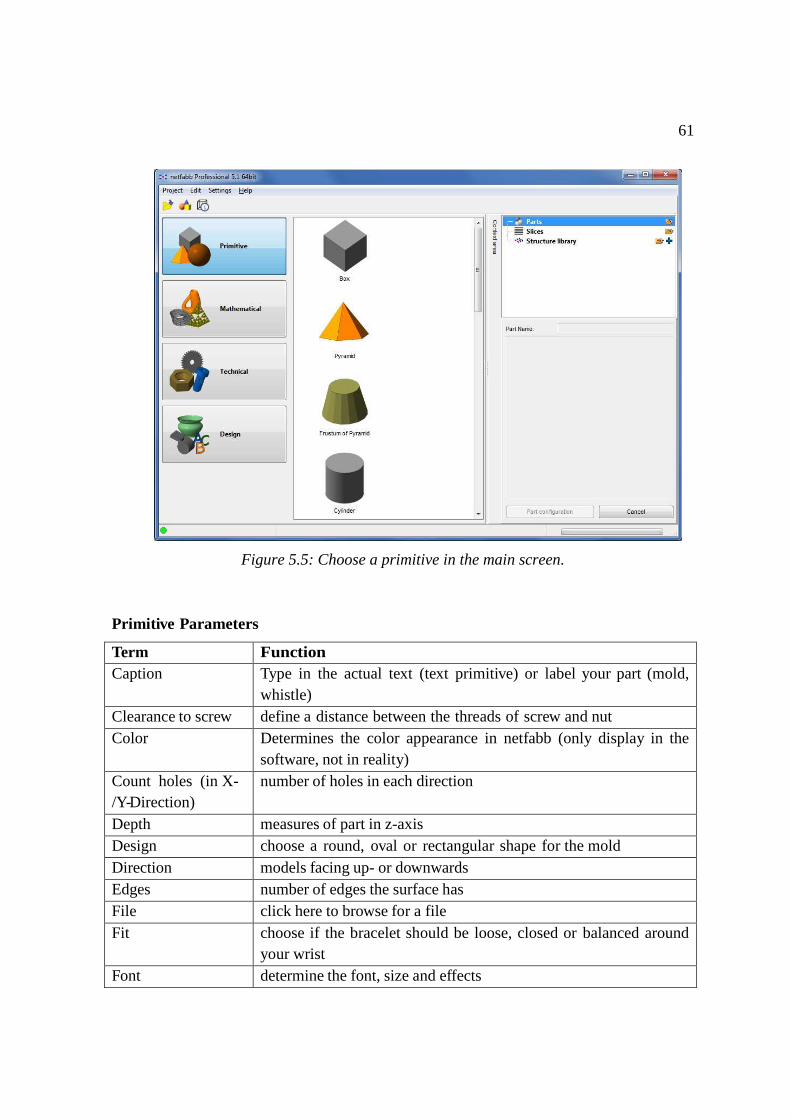
61
Figure 5.5: Choose a primitive in the main screen.
Primitive Parameters
Term Function Caption Type in the actual text (text primitive) or label your part (mold,
whistle) Clearance to screw define a distance between the threads of screw and nut Color Determines the color appearance in netfabb (only display in the
software, not in reality) Count holes (in X-/Y-Direction)
number of holes in each direction
Depth measures of part in z-axis Design choose a round, oval or rectangular shape for the mold Direction models facing up- or downwards Edges number of edges the surface has File click here to browse for a file Fit choose if the bracelet should be loose, closed or balanced around
your wrist Font determine the font, size and effects
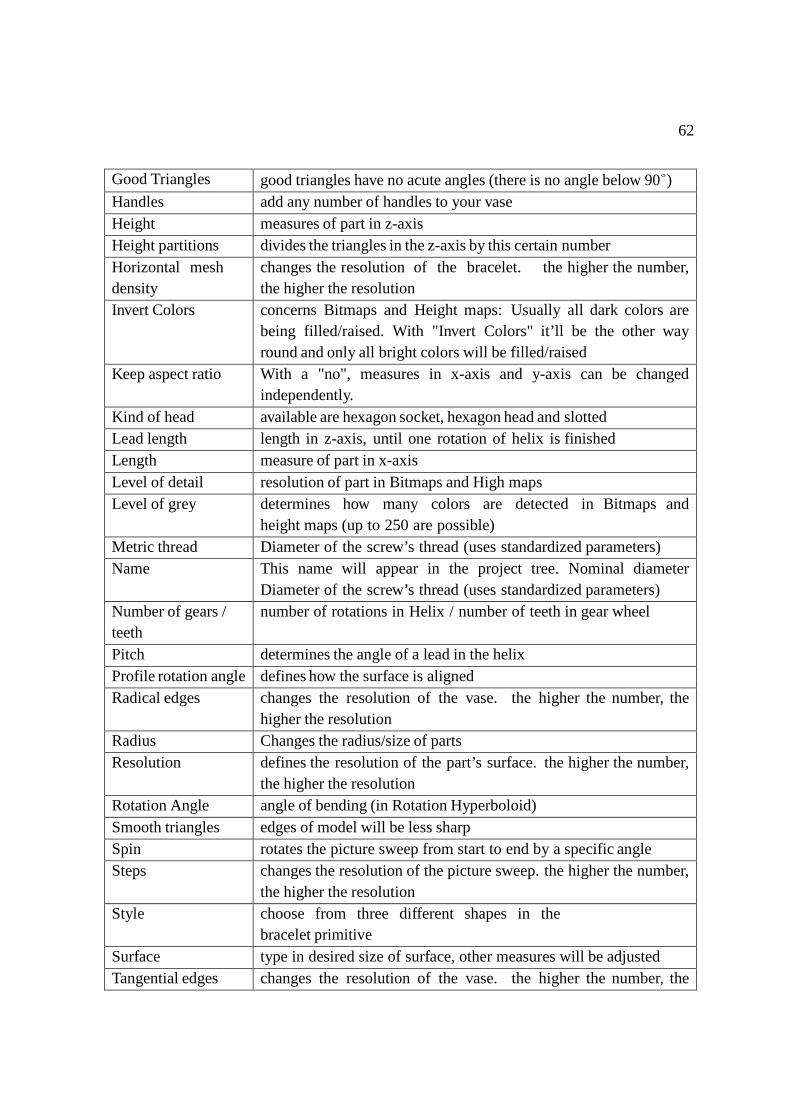
62
Good Triangles good triangles have no acute angles (there is no angle below 90◦) Handles add any number of handles to your vase Height measures of part in z-axis Height partitions divides the triangles in the z-axis by this certain number Horizontal mesh density
changes the resolution of the bracelet. the higher the number, the higher the resolution
Invert Colors concerns Bitmaps and Height maps: Usually all dark colors are being filled/raised. With "Invert Colors" it’ll be the other way round and only all bright colors will be filled/raised
Keep aspect ratio With a "no", measures in x-axis and y-axis can be changed independently.
Kind of head available are hexagon socket, hexagon head and slotted Lead length length in z-axis, until one rotation of helix is finished Length measure of part in x-axis Level of detail resolution of part in Bitmaps and High maps Level of grey determines how many colors are detected in Bitmaps and
height maps (up to 250 are possible) Metric thread Diameter of the screw’s thread (uses standardized parameters) Name This name will appear in the project tree. Nominal diameter
Diameter of the screw’s thread (uses standardized parameters) Number of gears / teeth
number of rotations in Helix / number of teeth in gear wheel
Pitch determines the angle of a lead in the helix Profile rotation angle defines how the surface is aligned Radical edges changes the resolution of the vase. the higher the number, the
higher the resolution Radius Changes the radius/size of parts Resolution defines the resolution of the part’s surface. the higher the number,
the higher the resolution Rotation Angle angle of bending (in Rotation Hyperboloid) Smooth triangles edges of model will be less sharp Spin rotates the picture sweep from start to end by a specific angle Steps changes the resolution of the picture sweep. the higher the number,
the higher the resolution Style choose from three different shapes in the
bracelet primitive Surface type in desired size of surface, other measures will be adjusted Tangential edges changes the resolution of the vase. the higher the number, the
63
higher the resolution Thickness of bars Width of each bar between two holes (in cylinder with hexagon
grid) Thread Length Length of the thread only, without head Tolerance A higher tolerance makes the roundness of parts less accurate and
results in a lower number of triangles. Triangle Edge Length
max. length of triangles edges
Triangles number of triangles Turns determines how many turns you need in your helix Type choose between predefined models Vertical mesh density
changes the resolution of the bracelet. the higher the number, the higher the resolution
Volume type in desired volume, other measures will be adjusted Wall thickness distance between inner and outer shell Width measures of part in y-axis Wrench size distance between two opposite edges of the outer nut contour Wrist circumference determines the inner circumference of the bracelet
5.4 Duplicate Parts
This feature can be accessed via the Part menu or in the context menu after right-
clicking on the respective part and creates a chosen number of exact copies of the
selected part. In a dialog box, you can set the overall number of copies. So, if you want to
create one duplicate, you have to set the counter to two copies.
Below, there is a little box Arrange Parts. If it is not ticked, the duplicates will be
placed in the same place as the original part. If it is ticked, you can place the duplicated
parts at specified positions next to the original part. Therefore, you can change the
number and the distance of duplicates in each direction (figure 5.6).

64
To define how many duplicates shall be arranged next to the original, you insert the
number of copies along all three axes. As this includes the original, the minimum
value is always one (even if you manually insert zero or a negative value, the count will be
one). The number of copies along the three axes is always adjusted when you change the
total count of copies.
If the box auto-adjust total count is not ticked and you change the number of copies
along one axis, the count of duplicates along the other axes is adjusted automatically so that
the number of total copies stays the same. If the box to the left of an axis is unticked, the
count along this axis will not be adjusted.
If the box "auto-adjust total count" is ticked and you change the number of copies along
one axis, the total count is automatically adjusted instead of the count along the other
axes.
Next, you can edit the distance of arranged copies along the three axes. The value you
enter always refers to the outbox of the parts. If you insert zero, the lowest coordinate value
of the second part will the same as the highest of the original/previous part. If you increase
Figure 5.6: Left: The dialog box for creating duplicates. Right: Duplicates of an ellipse-torus.
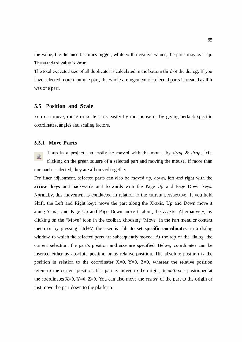
65
the value, the distance becomes bigger, while with negative values, the parts may overlap.
The standard value is 2mm.
The total expected size of all duplicates is calculated in the bottom third of the dialog. If you
have selected more than one part, the whole arrangement of selected parts is treated as if it
was one part.
5.5 Position and Scale
You can move, rotate or scale parts easily by the mouse or by giving netfabb specific
coordinates, angles and scaling factors.
5.5.1 Move Parts
Parts in a project can easily be moved with the mouse by drag & drop, left-
clicking on the green square of a selected part and moving the mouse. If more than
one part is selected, they are all moved together.
For finer adjustment, selected parts can also be moved up, down, left and right with the
arrow keys and backwards and forwards with the Page Up and Page Down keys.
Normally, this movement is conducted in relation to the current perspective. If you hold
Shift, the Left and Right keys move the part along the X-axis, Up and Down move it
along Y-axis and Page Up and Page Down move it along the Z-axis. Alternatively, by
clicking on the "Move" icon in the toolbar, choosing "Move" in the Part menu or context
menu or by pressing Ctrl+V, the user is able to set specific coordinates in a dialog
window, to which the selected parts are subsequently moved. At the top of the dialog, the
current selection, the part’s position and size are specified. Below, coordinates can be
inserted either as absolute position or as relative position. The absolute position is the
position in relation to the coordinates X=0, Y=0, Z=0, whereas the relative position
refers to the current position. If a part is moved to the origin, its outbox is positioned at
the coordinates X=0, Y=0, Z=0. You can also move the center of the part to the origin or
just move the part down to the platform.

66
Figure 5.7: The dialog box for moving parts
If the box Keep window open is ticked, you can apply the changes by "Translate", the
dialog will stay open and you immediately can move the part again. (figure 5.7).
5.5.2 Rotate Parts
Similarly to moving parts, they can also be rotated easily with the mouse. This is
performed by left-clicking on the green brackets of selected parts, holding the
mouse button and moving the mouse in the direction in which you want to turn the part.
Thereby, the axis of rotation is normally the direction from which the part is seen, but if you
hold Ctrl, the part is rotated around the closest main axis (figure 5.8). With pressing the
ALT key, the part will be rotated in 10° steps (value adjustable in the program settings).
Hit the keys X, Y or Z and the part is rotated by 45° clockwise, with Shift counterwise
(value adjustable in the program settings). This function is available in the toolbar, in the
Part menu or by pressing Ctrl+R.
Figure 5.8: Click on the green brackets and move the mouse to rotate a part.
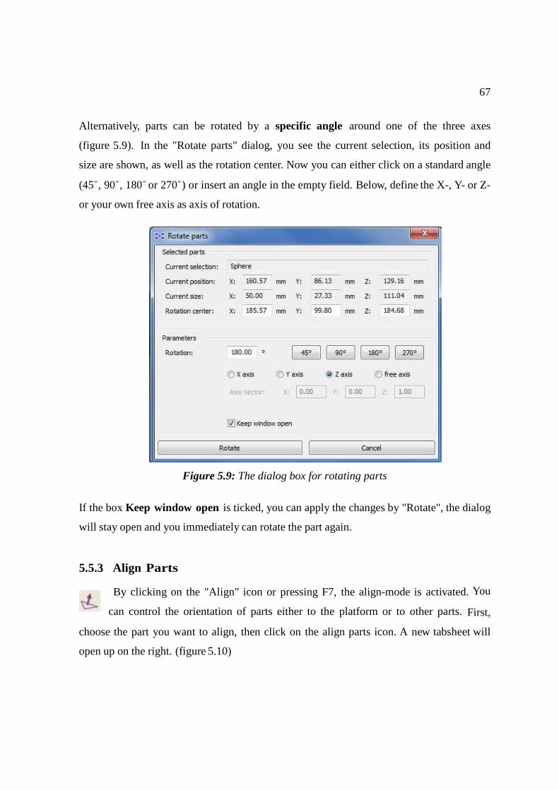
67
Alternatively, parts can be rotated by a specific angle around one of the three axes
(figure 5.9). In the "Rotate parts" dialog, you see the current selection, its position and
size are shown, as well as the rotation center. Now you can either click on a standard angle
(45◦, 90◦, 180◦ or 270◦) or insert an angle in the empty field. Below, define the X-, Y- or Z-
or your own free axis as axis of rotation.
Figure 5.9: The dialog box for rotating parts
If the box Keep window open is ticked, you can apply the changes by "Rotate", the dialog
will stay open and you immediately can rotate the part again.
5.5.3 Align Parts
By clicking on the "Align" icon or pressing F7, the align-mode is activated. You
can control the orientation of parts either to the platform or to other parts. First,
choose the part you want to align, then click on the align parts icon. A new tabsheet will
open up on the right. (figure 5.10)
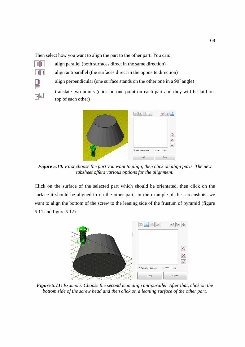
68
Then select how you want to align the part to the other part. You can:
align parallel (both surfaces direct in the same direction)
align antiparallel (the surfaces direct in the opposite direction)
align perpendicular (one surface stands on the other one in a 90◦ angle)
translate two points (click on one point on each part and they will be laid on
top of each other)
Figure 5.10: First choose the part you want to align, then click on align parts. The new tabsheet offers various options for the alignment.
Click on the surface of the selected part which should be orientated, then click on the
surface it should be aligned to on the other part. In the example of the screenshots, we
want to align the bottom of the screw to the leaning side of the frustum of pyramid (figure
5.11 and figure 5.12).
Figure 5.11: Example: Choose the second icon align antiparallel. After that, click on the bottom side of the screw head and then click on a leaning surface of the other part.
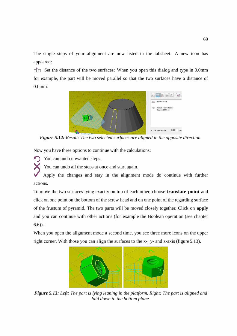
69
The single steps of your alignment are now listed in the tabsheet. A new icon has
appeared:
Set the distance of the two surfaces: When you open this dialog and type in 0.0mm
for example, the part will be moved parallel so that the two surfaces have a distance of
0.0mm.
Figure 5.12: Result: The two selected surfaces are aligned in the opposite direction.
Now you have three options to continue with the calculations:
You can undo unwanted steps.
You can undo all the steps at once and start again.
Apply the changes and stay in the alignment mode do continue with further
actions.
To move the two surfaces lying exactly on top of each other, choose translate point and
click on one point on the bottom of the screw head and on one point of the regarding surface
of the frustum of pyramid. The two parts will be moved closely together. Click on apply
and you can continue with other actions (for example the Boolean operation (see chapter
6.6)).
When you open the alignment mode a second time, you see three more icons on the upper
right corner. With those you can align the surfaces to the x-, y- and z-axis (figure 5.13).
Figure 5.13: Left: The part is lying leaning in the platform. Right: The part is aligned and laid down to the bottom plane.
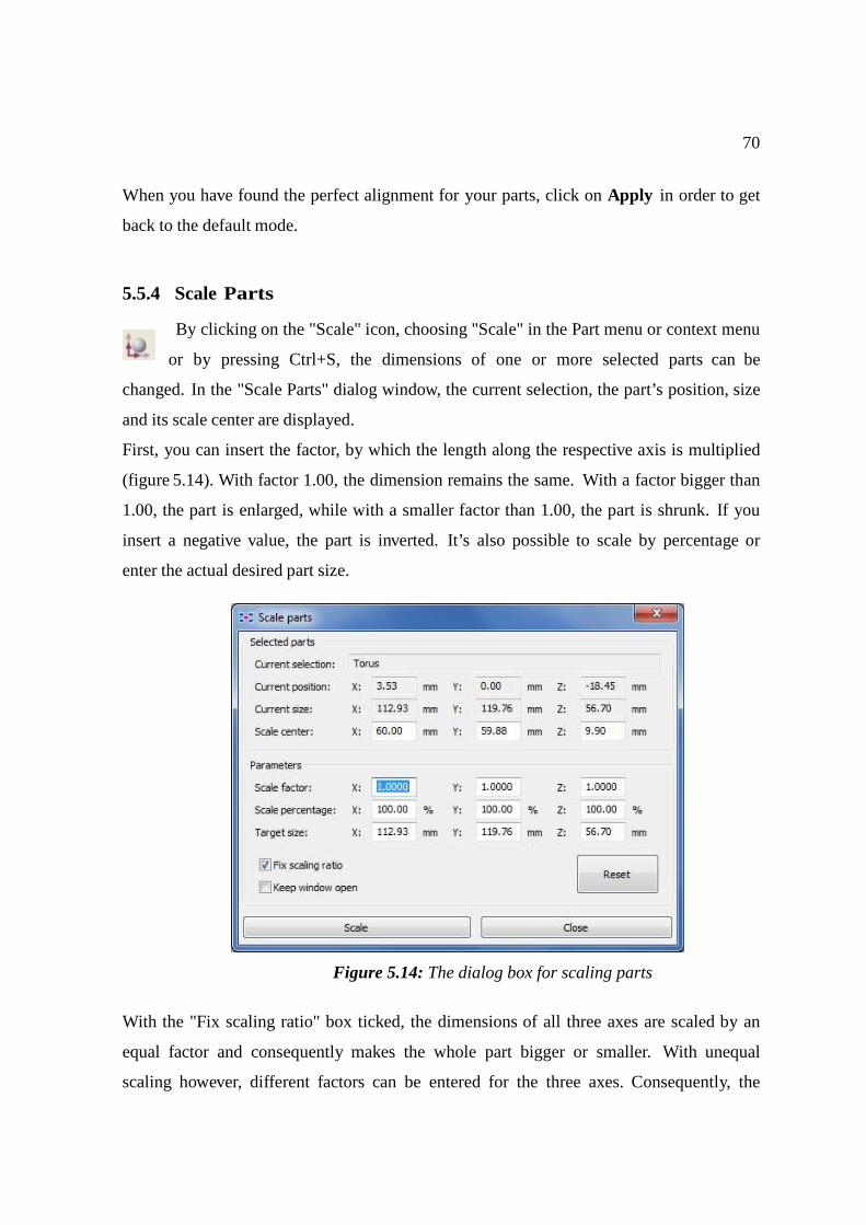
70
When you have found the perfect alignment for your parts, click on Apply in order to get
back to the default mode.
5.5.4 Scale Parts
By clicking on the "Scale" icon, choosing "Scale" in the Part menu or context menu
or by pressing Ctrl+S, the dimensions of one or more selected parts can be
changed. In the "Scale Parts" dialog window, the current selection, the part’s position, size
and its scale center are displayed.
First, you can insert the factor, by which the length along the respective axis is multiplied
(figure 5.14). With factor 1.00, the dimension remains the same. With a factor bigger than
1.00, the part is enlarged, while with a smaller factor than 1.00, the part is shrunk. If you
insert a negative value, the part is inverted. It’s also possible to scale by percentage or
enter the actual desired part size.
Figure 5.14: The dialog box for scaling parts
With the "Fix scaling ratio" box ticked, the dimensions of all three axes are scaled by an
equal factor and consequently makes the whole part bigger or smaller. With unequal
scaling however, different factors can be entered for the three axes. Consequently, the
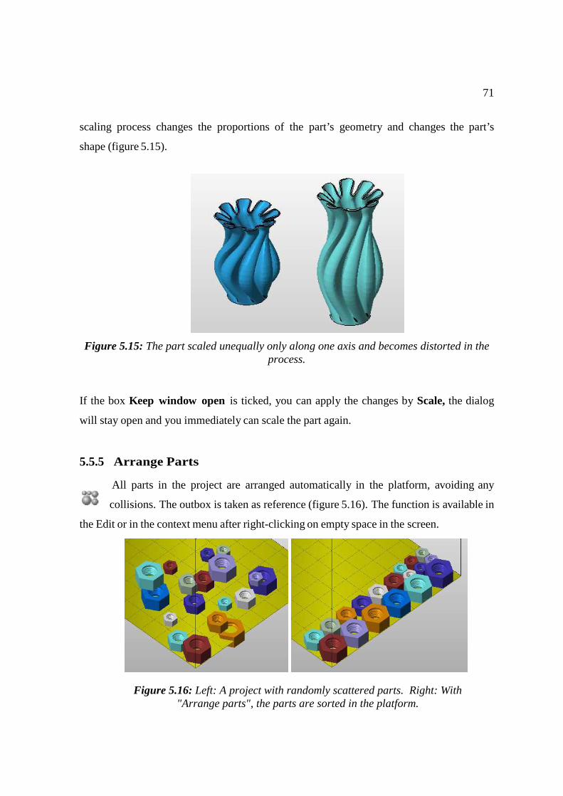
71
scaling process changes the proportions of the part’s geometry and changes the part’s
shape (figure 5.15).
Figure 5.15: The part scaled unequally only along one axis and becomes distorted in the process.
If the box Keep window open is ticked, you can apply the changes by Scale, the dialog
will stay open and you immediately can scale the part again.
5.5.5 Arrange Parts
All parts in the project are arranged automatically in the platform, avoiding any
collisions. The outbox is taken as reference (figure 5.16). The function is available in
the Edit or in the context menu after right-clicking on empty space in the screen.
Figure 5.16: Left: A project with randomly scattered parts. Right: With "Arrange parts", the parts are sorted in the platform.
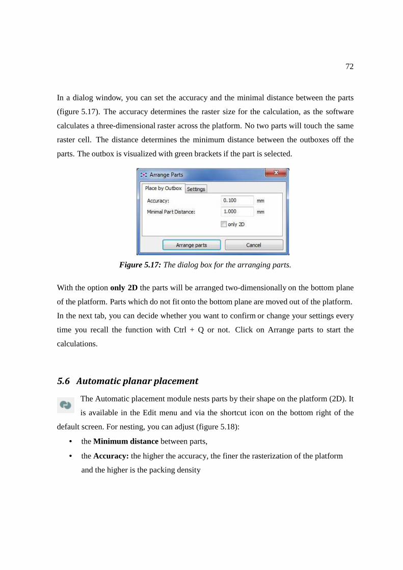
72
In a dialog window, you can set the accuracy and the minimal distance between the parts
(figure 5.17). The accuracy determines the raster size for the calculation, as the software
calculates a three-dimensional raster across the platform. No two parts will touch the same
raster cell. The distance determines the minimum distance between the outboxes off the
parts. The outbox is visualized with green brackets if the part is selected.
Figure 5.17: The dialog box for the arranging parts.
With the option only 2D the parts will be arranged two-dimensionally on the bottom plane
of the platform. Parts which do not fit onto the bottom plane are moved out of the platform.
In the next tab, you can decide whether you want to confirm or change your settings every
time you recall the function with Ctrl + Q or not. Click on Arrange parts to start the
calculations.
5.6 Automatic planar placement
The Automatic placement module nests parts by their shape on the platform (2D). It
is available in the Edit menu and via the shortcut icon on the bottom right of the
default screen. For nesting, you can adjust (figure 5.18):
• the Minimum distance between parts,
• the Accuracy: the higher the accuracy, the finer the rasterization of the platform
and the higher is the packing density
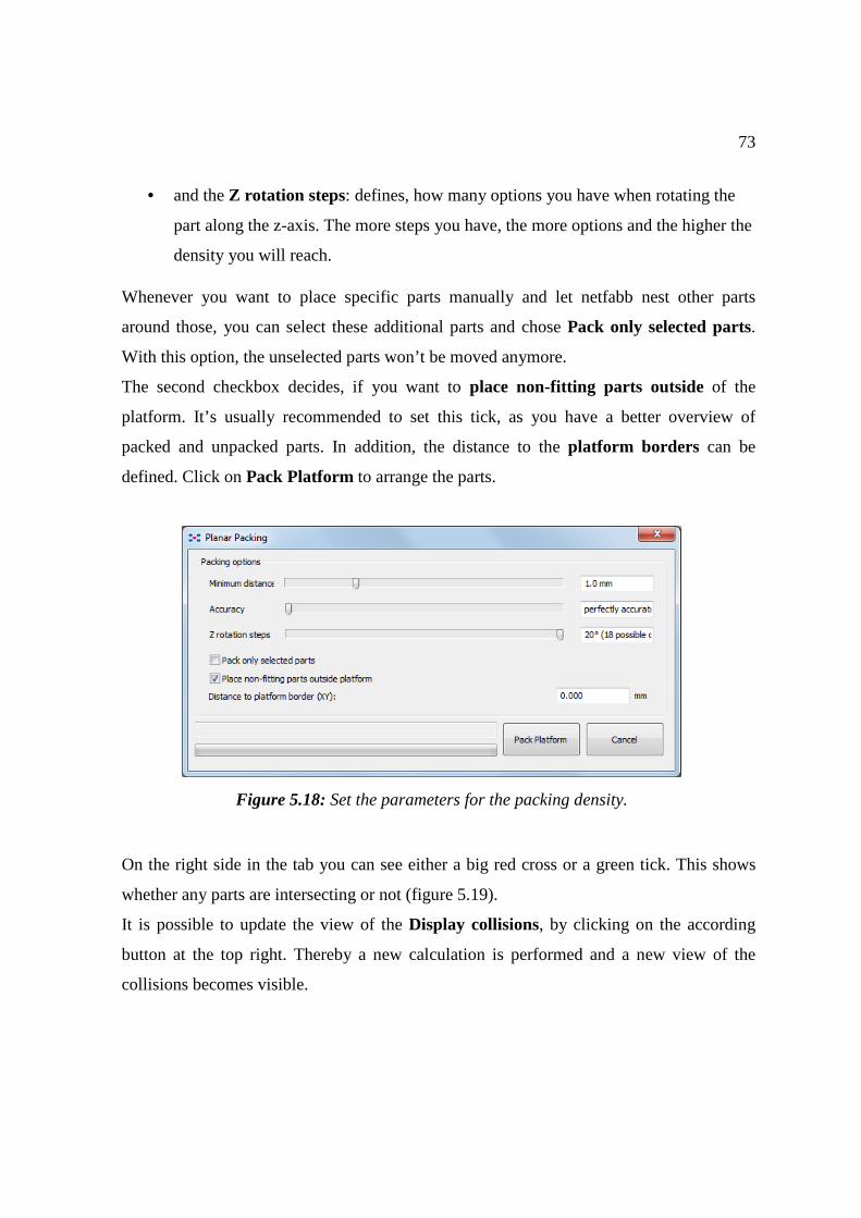
73
• and the Z rotation steps: defines, how many options you have when rotating the
part along the z-axis. The more steps you have, the more options and the higher the
density you will reach.
Whenever you want to place specific parts manually and let netfabb nest other parts
around those, you can select these additional parts and chose Pack only selected parts.
With this option, the unselected parts won’t be moved anymore.
The second checkbox decides, if you want to place non-fitting parts outside of the
platform. It’s usually recommended to set this tick, as you have a better overview of
packed and unpacked parts. In addition, the distance to the platform borders can be
defined. Click on Pack Platform to arrange the parts.
On the right side in the tab you can see either a big red cross or a green tick. This shows
whether any parts are intersecting or not (figure 5.19).
It is possible to update the view of the Display collisions, by clicking on the according
button at the top right. Thereby a new calculation is performed and a new view of the
collisions becomes visible.
Figure 5.18: Set the parameters for the packing density.
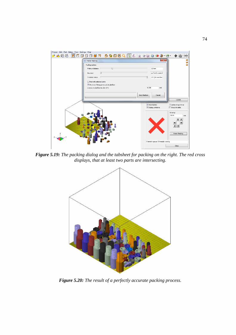
74
Figure 5.19: The packing dialog and the tabsheet for packing on the right. The red cross displays, that at least two parts are intersecting.
Figure 5.20: The result of a perfectly accurate packing process.
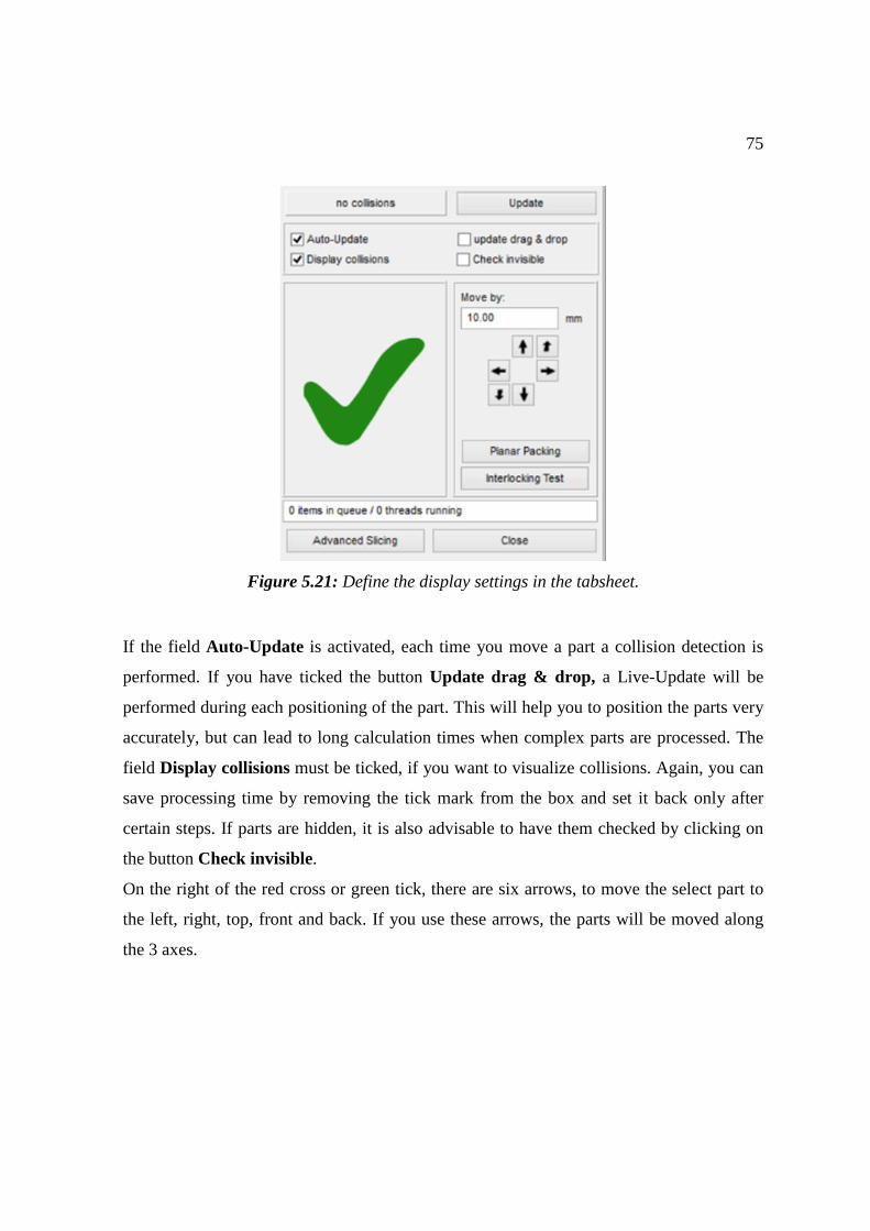
75
Figure 5.21: Define the display settings in the tabsheet.
If the field Auto-Update is activated, each time you move a part a collision detection is
performed. If you have ticked the button Update drag & drop, a Live-Update will be
performed during each positioning of the part. This will help you to position the parts very
accurately, but can lead to long calculation times when complex parts are processed. The
field Display collisions must be ticked, if you want to visualize collisions. Again, you can
save processing time by removing the tick mark from the box and set it back only after
certain steps. If parts are hidden, it is also advisable to have them checked by clicking on
the button Check invisible.
On the right of the red cross or green tick, there are six arrows, to move the select part to
the left, right, top, front and back. If you use these arrows, the parts will be moved along
the 3 axes.
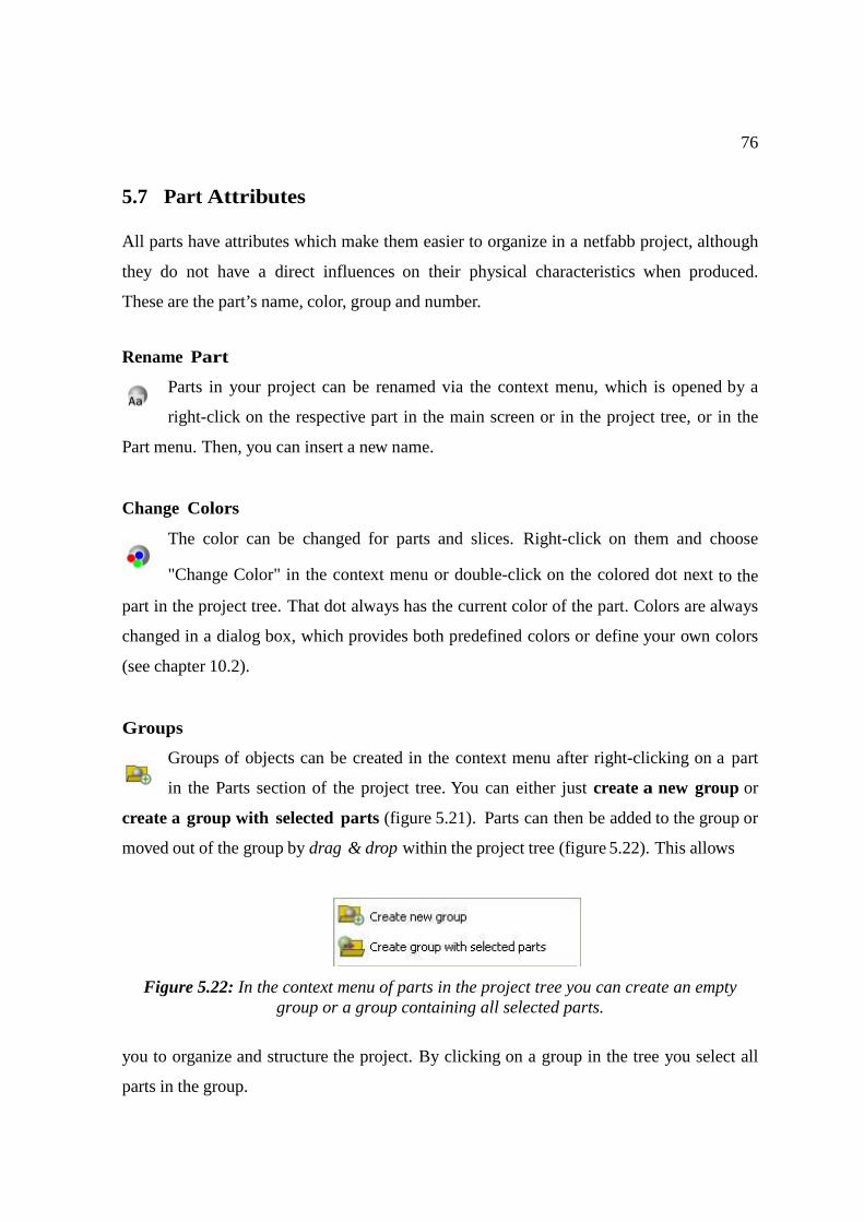
76
5.7 Part Attributes
All parts have attributes which make them easier to organize in a netfabb project, although
they do not have a direct influences on their physical characteristics when produced.
These are the part’s name, color, group and number. Rename Part
Parts in your project can be renamed via the context menu, which is opened by a
right-click on the respective part in the main screen or in the project tree, or in the
Part menu. Then, you can insert a new name.
Change Colors
The color can be changed for parts and slices. Right-click on them and choose
"Change Color" in the context menu or double-click on the colored dot next to the
part in the project tree. That dot always has the current color of the part. Colors are always
changed in a dialog box, which provides both predefined colors or define your own colors
(see chapter 10.2).
Groups
Groups of objects can be created in the context menu after right-clicking on a part
in the Parts section of the project tree. You can either just create a new group or
create a group with selected parts (figure 5.21). Parts can then be added to the group or
moved out of the group by drag & drop within the project tree (figure 5.22). This allows
Figure 5.22: In the context menu of parts in the project tree you can create an empty group or a group containing all selected parts.
you to organize and structure the project. By clicking on a group in the tree you select all
parts in the group.
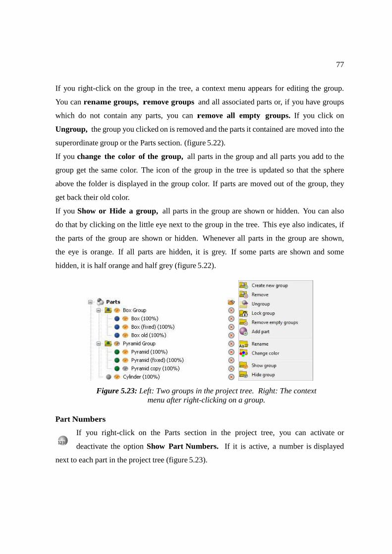
77
If you right-click on the group in the tree, a context menu appears for editing the group.
You can rename groups, remove groups and all associated parts or, if you have groups
which do not contain any parts, you can remove all empty groups. If you click on
Ungroup, the group you clicked on is removed and the parts it contained are moved into the
superordinate group or the Parts section. (figure 5.22).
If you change the color of the group, all parts in the group and all parts you add to the
group get the same color. The icon of the group in the tree is updated so that the sphere
above the folder is displayed in the group color. If parts are moved out of the group, they
get back their old color.
If you Show or Hide a group, all parts in the group are shown or hidden. You can also
do that by clicking on the little eye next to the group in the tree. This eye also indicates, if
the parts of the group are shown or hidden. Whenever all parts in the group are shown,
the eye is orange. If all parts are hidden, it is grey. If some parts are shown and some
hidden, it is half orange and half grey (figure 5.22).
Part Numbers
If you right-click on the Parts section in the project tree, you can activate or
deactivate the option Show Part Numbers. If it is active, a number is displayed
next to each part in the project tree (figure 5.23).
Figure 5.23: Left: Two groups in the project tree. Right: The context menu after right-clicking on a group.
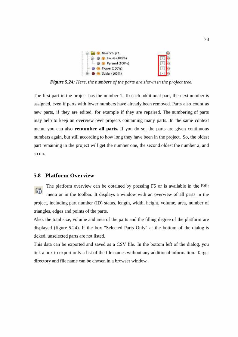
78
Figure 5.24: Here, the numbers of the parts are shown in the project tree.
The first part in the project has the number 1. To each additional part, the next number is
assigned, even if parts with lower numbers have already been removed. Parts also count as
new parts, if they are edited, for example if they are repaired. The numbering of parts
may help to keep an overview over projects containing many parts. In the same context
menu, you can also renumber all parts. If you do so, the parts are given continuous
numbers again, but still according to how long they have been in the project. So, the oldest
part remaining in the project will get the number one, the second oldest the number 2, and
so on.
5.8 Platform Overview
The platform overview can be obtained by pressing F5 or is available in the Edit
menu or in the toolbar. It displays a window with an overview of all parts in the
project, including part number (ID) status, length, width, height, volume, area, number of
triangles, edges and points of the parts.
Also, the total size, volume and area of the parts and the filling degree of the platform are
displayed (figure 5.24). If the box "Selected Parts Only" at the bottom of the dialog is
ticked, unselected parts are not listed.
This data can be exported and saved as a CSV file. In the bottom left of the dialog, you
tick a box to export only a list of the file names without any additional information. Target
directory and file name can be chosen in a browser window.
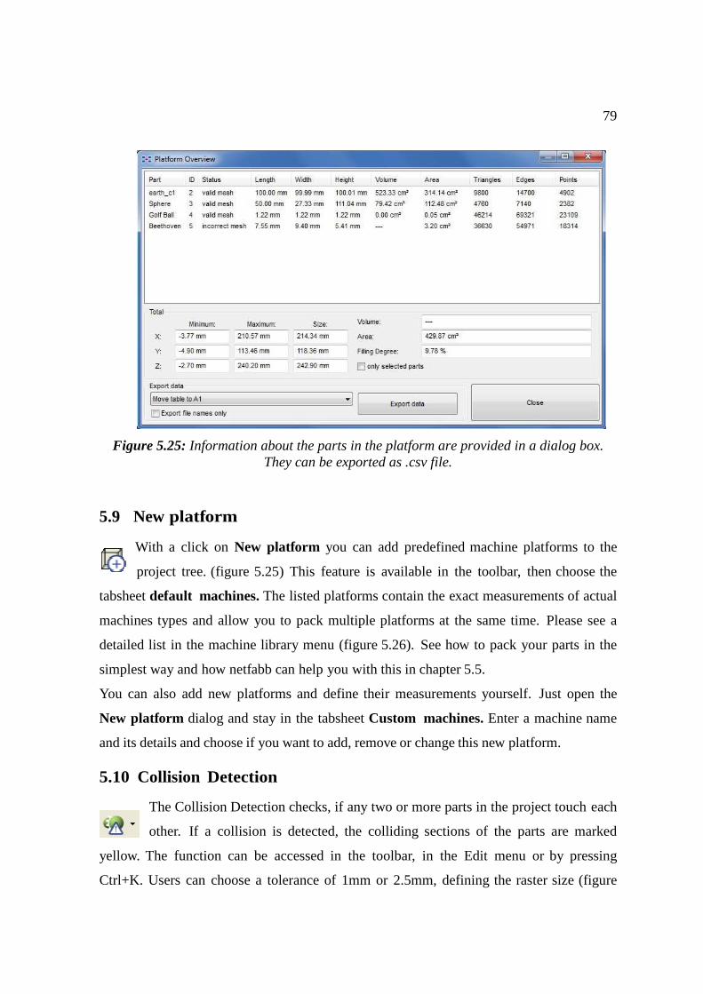
79
Figure 5.25: Information about the parts in the platform are provided in a dialog box. They can be exported as .csv file.
5.9 New platform
With a click on New platform you can add predefined machine platforms to the
project tree. (figure 5.25) This feature is available in the toolbar, then choose the
tabsheet default machines. The listed platforms contain the exact measurements of actual
machines types and allow you to pack multiple platforms at the same time. Please see a
detailed list in the machine library menu (figure 5.26). See how to pack your parts in the
simplest way and how netfabb can help you with this in chapter 5.5.
You can also add new platforms and define their measurements yourself. Just open the
New platform dialog and stay in the tabsheet Custom machines. Enter a machine name
and its details and choose if you want to add, remove or change this new platform.
5.10 Collision Detection
The Collision Detection checks, if any two or more parts in the project touch each
other. If a collision is detected, the colliding sections of the parts are marked
yellow. The function can be accessed in the toolbar, in the Edit menu or by pressing
Ctrl+K. Users can choose a tolerance of 1mm or 2.5mm, defining the raster size (figure
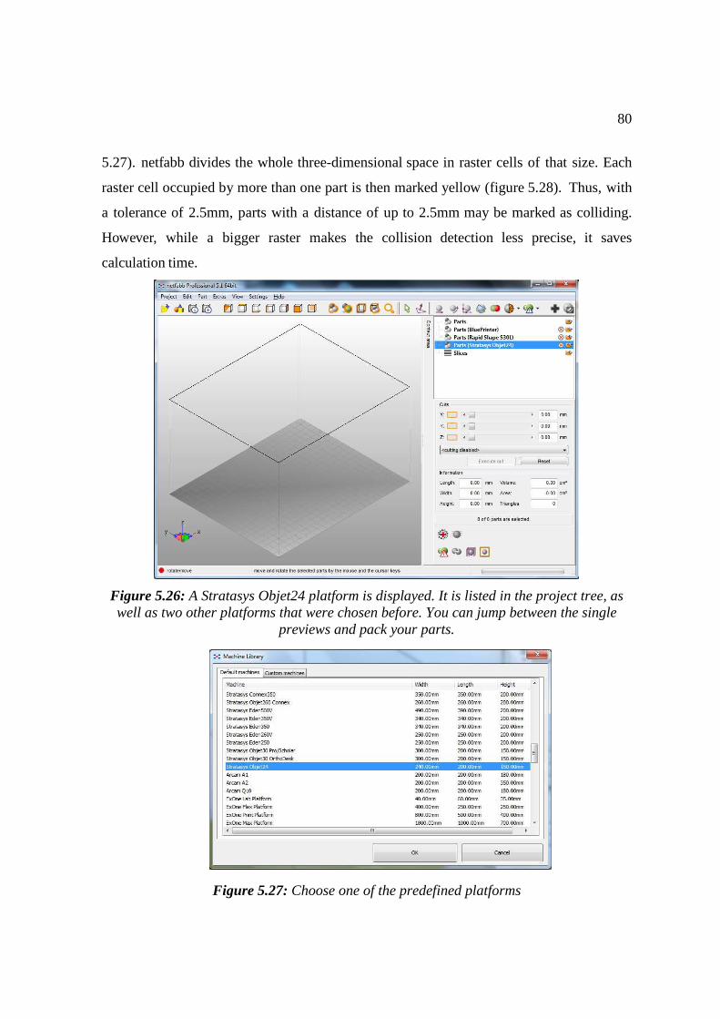
80
5.27). netfabb divides the whole three-dimensional space in raster cells of that size. Each
raster cell occupied by more than one part is then marked yellow (figure 5.28). Thus, with
a tolerance of 2.5mm, parts with a distance of up to 2.5mm may be marked as colliding.
However, while a bigger raster makes the collision detection less precise, it saves
calculation time.
Figure 5.26: A Stratasys Objet24 platform is displayed. It is listed in the project tree, as well as two other platforms that were chosen before. You can jump between the single
previews and pack your parts.
Figure 5.27: Choose one of the predefined platforms

81
Figure 5.28: Choose a tolerance of 1mm or 2.5mm.
5.10.1 Live Collision Detection
For the "Live Collision Detection", you can click on a button in the tabsheet to
activate it. netfabb then constantly checks your parts for collisions, which are
marked yellow in the screen. The raster size is always 1mm. A new tabsheet appears with
all options for the tool.
Operations in the viewing screen, such as the positioning and scaling of parts can be
conducted normally. As soon as two parts touch each other, the collision is marked and a
large red X is displayed in the tabsheet. As long as there is no collision, a green check is
displayed.
In the tabsheet you can change all settings for the collision detection and for the
positioning of parts (figure 5.33).
In the top left, there is a notice if a collision has been detected. To update the collision
detection, click on the button in the top right of the tabsheet. This will activate a new
calculation and a new highlighting of collisions in the viewing screen. If you tick the box
Auto-update, an update will be performed every time you move of a part. If you tick the
Figure 5.29: Left: Collisions are marked yellow. Right: Zoom in to see the marked raster cells.
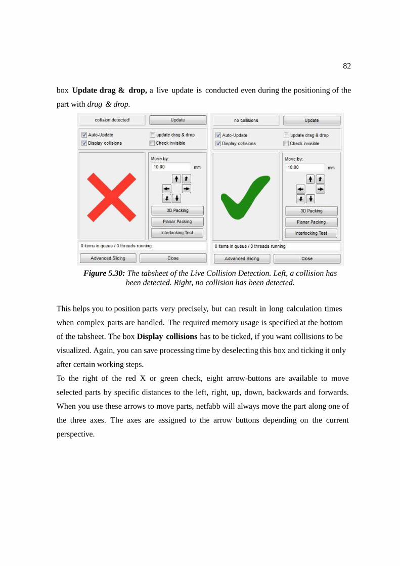
82
box Update drag & drop, a live update is conducted even during the positioning of the
part with drag & drop.
This helps you to position parts very precisely, but can result in long calculation times
when complex parts are handled. The required memory usage is specified at the bottom
of the tabsheet. The box Display collisions has to be ticked, if you want collisions to be
visualized. Again, you can save processing time by deselecting this box and ticking it only
after certain working steps.
To the right of the red X or green check, eight arrow-buttons are available to move
selected parts by specific distances to the left, right, up, down, backwards and forwards.
When you use these arrows to move parts, netfabb will always move the part along one of
the three axes. The axes are assigned to the arrow buttons depending on the current
perspective.
Figure 5.30: The tabsheet of the Live Collision Detection. Left, a collision has been detected. Right, no collision has been detected.
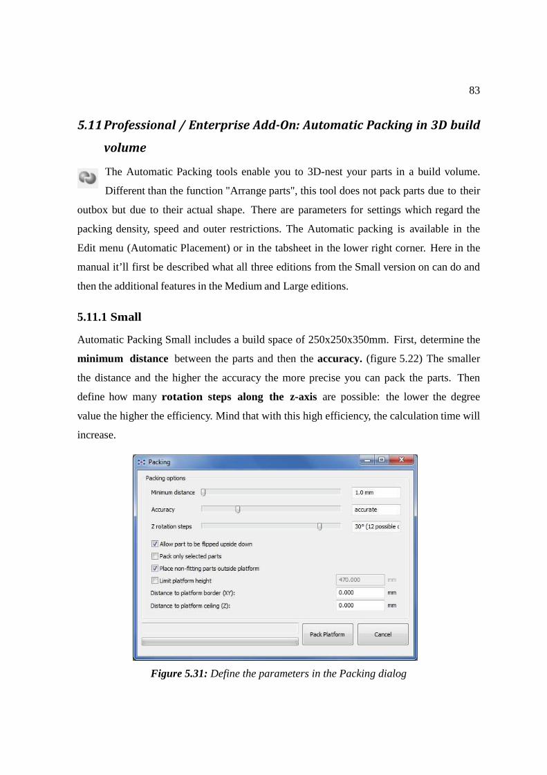
83
5.11 Professional / Enterprise Add-On: Automatic Packing in 3D build
volume
The Automatic Packing tools enable you to 3D-nest your parts in a build volume.
Different than the function "Arrange parts", this tool does not pack parts due to their
outbox but due to their actual shape. There are parameters for settings which regard the
packing density, speed and outer restrictions. The Automatic packing is available in the
Edit menu (Automatic Placement) or in the tabsheet in the lower right corner. Here in the
manual it’ll first be described what all three editions from the Small version on can do and
then the additional features in the Medium and Large editions.
5.11.1 Small
Automatic Packing Small includes a build space of 250x250x350mm. First, determine the
minimum distance between the parts and then the accuracy. (figure 5.22) The smaller
the distance and the higher the accuracy the more precise you can pack the parts. Then
define how many rotation steps along the z-axis are possible: the lower the degree
value the higher the efficiency. Mind that with this high efficiency, the calculation time will
increase.
Figure 5.31: Define the parameters in the Packing dialog
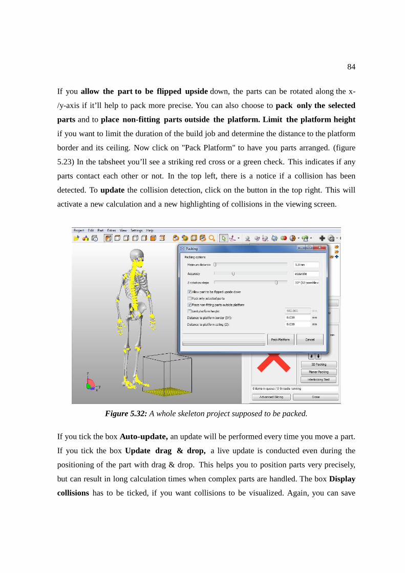
84
If you allow the part to be flipped upside down, the parts can be rotated along the x-
/y-axis if it’ll help to pack more precise. You can also choose to pack only the selected
parts and to place non-fitting parts outside the platform. Limit the platform height
if you want to limit the duration of the build job and determine the distance to the platform
border and its ceiling. Now click on "Pack Platform" to have you parts arranged. (figure
5.23) In the tabsheet you’ll see a striking red cross or a green check. This indicates if any
parts contact each other or not. In the top left, there is a notice if a collision has been
detected. To update the collision detection, click on the button in the top right. This will
activate a new calculation and a new highlighting of collisions in the viewing screen.
Figure 5.32: A whole skeleton project supposed to be packed.
If you tick the box Auto-update, an update will be performed every time you move a part.
If you tick the box Update drag & drop, a live update is conducted even during the
positioning of the part with drag & drop. This helps you to position parts very precisely,
but can result in long calculation times when complex parts are handled. The box Display
collisions has to be ticked, if you want collisions to be visualized. Again, you can save
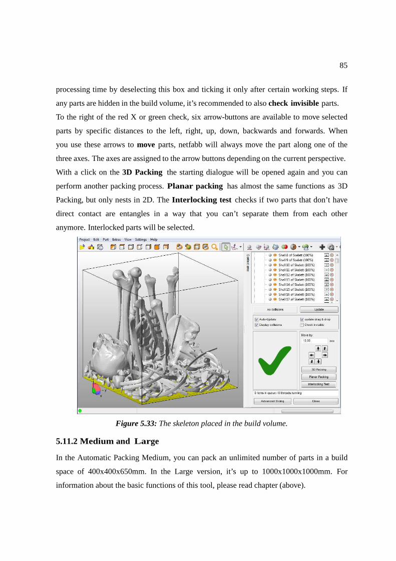
85
processing time by deselecting this box and ticking it only after certain working steps. If
any parts are hidden in the build volume, it’s recommended to also check invisible parts.
To the right of the red X or green check, six arrow-buttons are available to move selected
parts by specific distances to the left, right, up, down, backwards and forwards. When
you use these arrows to move parts, netfabb will always move the part along one of the
three axes. The axes are assigned to the arrow buttons depending on the current perspective.
With a click on the 3D Packing the starting dialogue will be opened again and you can
perform another packing process. Planar packing has almost the same functions as 3D
Packing, but only nests in 2D. The Interlocking test checks if two parts that don’t have
direct contact are entangles in a way that you can’t separate them from each other
anymore. Interlocked parts will be selected.
Figure 5.33: The skeleton placed in the build volume.
5.11.2 Medium and Large
In the Automatic Packing Medium, you can pack an unlimited number of parts in a build
space of 400x400x650mm. In the Large version, it’s up to 1000x1000x1000mm. For
information about the basic functions of this tool, please read chapter (above).
86
For a direct slice output for EOS machines, click on Advanced Slicing. Parts and
platform constraints are checked again. The EOS SLI format is chosen already, then enter
the desired filename and the layer size. Enable Slice reduction with tolerance? If you have
a lot of very small parts, it’s recommended to use model packages so they can’t get lost in
the build space. For that, select all the parts you want to join in a package and move them
close together. The press the button Create model package in the Part menu or in the default
mode in the bottom right corner.
In the Large Packing version, there’s also a Data-API to save and open packed build
spaces in a network and an integration of an ERP System. Manuals and support will be
given individually.
87
6 Part Edit
Three-dimensional parts can be edited in various ways. Features include the analysis of
parts, simple part editing functions, such as mirroring, inverting and converting in size
according to the length units mm an inch and the conducting of simple cuts. Furthermore,
any number of parts can be merged to one part and any part consisting of more than one
shell can be split into equivalent parts. Also, new shells and offsets can be created on the
basis of existing objects, cutting planes can be defined freely and parts can be unified,
subtracted or an intersection of parts can be created with the Boolean Operations Module.
Further part editing functions are part of the repair module (chapter 7.1). These are
features for which you have to work with the triangle mesh more specifically.
6.1 Part Analysis
For the analysis of a part you have five options. A standard analysis, an analysis of
upskins and downskins, of the center of gravity, the wall thickness and the
analysis of the part’s shadow area. For users, who have purchased netfabb Professional
before version 4.7, only the standard analysis might be visible because of license issues. In
that case, please contact us at [email protected]. You will get a new license file to
activate the two analysis options.
An analysis of a selected part can be obtained by a click on the analysis icon in the
toolbar, in the Extras menu or in the Extras submenu of the context menu of a part. You
get a submenu where you can choose from the three kinds of analyses.
The analysis opens a window in the tabsheet providing information on the part. The
content depends on which analysis you have chosen. Information on all of your analyses
is listed together (figure 6.1). In the project tree, a folder "Part analysis" is added as sub
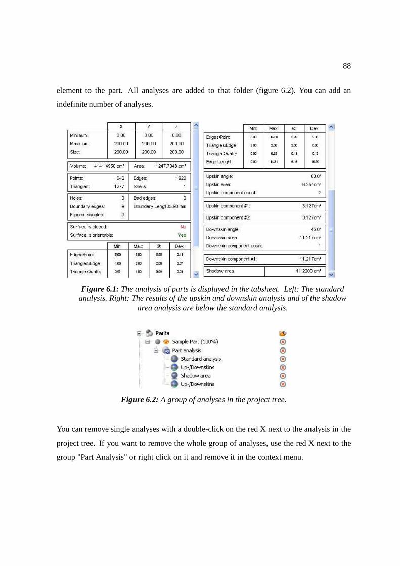
88
element to the part. All analyses are added to that folder (figure 6.2). You can add an
indefinite number of analyses.
Figure 6.2: A group of analyses in the project tree.
You can remove single analyses with a double-click on the red X next to the analysis in the
project tree. If you want to remove the whole group of analyses, use the red X next to the
group "Part Analysis" or right click on it and remove it in the context menu.
Figure 6.1: The analysis of parts is displayed in the tabsheet. Left: The standard analysis. Right: The results of the upskin and downskin analysis and of the shadow
area analysis are below the standard analysis.
89
6.1.1 Standard Analysis
The standard analysis provides information on the position, size, volume and area of
a selected part, as well as its number of points, triangles, edges and shells. It
provides information about potential damage to the part by showing the number of holes,
boundary edges, flipped triangles and bad edges, specifies the overall length of boundary
edges and checks, if the part is closed and orientable. Thus, you can find out, if a part
requires repair and which kind of repair it requires.
Additionally, the minimum, maximum and average value as well as the deviation are
calculated and specified for edges per point, triangles per edge, triangle quality and edge
length (figure 6.1).
6.1.2 Upskin and Downskin Analysis
If you choose the analysis of up/downskins, you can identify the top and bottom
surfaces of your part. You find out precisely, which surface areas of your part are
below a certain angle in relation to the bottom plane of the platform (X-Y- plane). All
areas below this angle are either an upskin or a downskin, depending on their orientation
upwards or downwards.
This analysis can be very important, as, for example, some production methods have a
different quality for upskins and downskins and it may make sense to rotate parts to
minimize those areas.
In a dialog box, you can enter the settings for the up/downskin analysis. First, you can
tick boxes to analyze upskins, downskins or both.
To the right, enter the threshold angles. If you enter 0◦, only absolutely flat areas will be
defined as upskins and downskins. If you enter 90◦, everything between the flat areas and
horizontal planes are defined as upskins or downskins.
In the parameters, you can edit the minimum component size and choose to filter small
triangles:
The minimum component size determines how big the upskin or downskin areas must
be. Sometimes, it is possible that very small areas, for example single triangles, are within
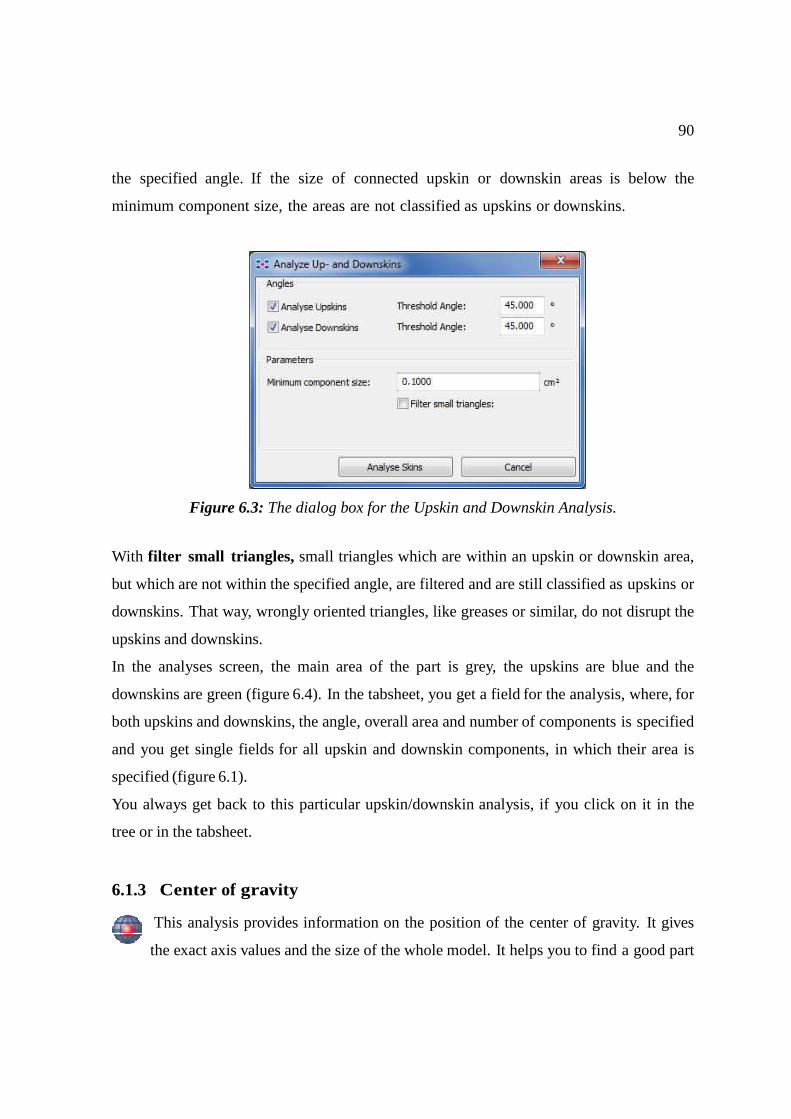
90
the specified angle. If the size of connected upskin or downskin areas is below the
minimum component size, the areas are not classified as upskins or downskins.
Figure 6.3: The dialog box for the Upskin and Downskin Analysis.
With filter small triangles, small triangles which are within an upskin or downskin area,
but which are not within the specified angle, are filtered and are still classified as upskins or
downskins. That way, wrongly oriented triangles, like greases or similar, do not disrupt the
upskins and downskins.
In the analyses screen, the main area of the part is grey, the upskins are blue and the
downskins are green (figure 6.4). In the tabsheet, you get a field for the analysis, where, for
both upskins and downskins, the angle, overall area and number of components is specified
and you get single fields for all upskin and downskin components, in which their area is
specified (figure 6.1).
You always get back to this particular upskin/downskin analysis, if you click on it in the
tree or in the tabsheet.
6.1.3 Center of gravity
This analysis provides information on the position of the center of gravity. It gives
the exact axis values and the size of the whole model. It helps you to find a good part
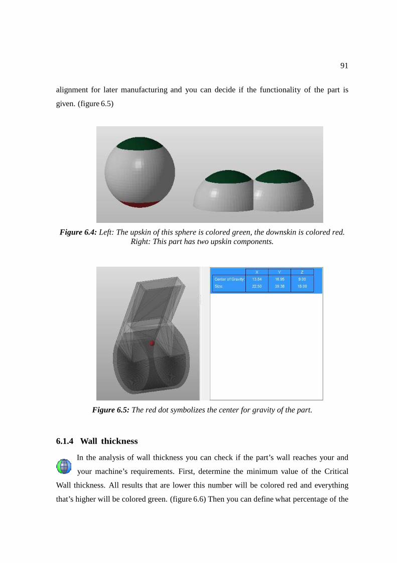
91
alignment for later manufacturing and you can decide if the functionality of the part is
given. (figure 6.5)
Figure 6.4: Left: The upskin of this sphere is colored green, the downskin is colored red. Right: This part has two upskin components.
Figure 6.5: The red dot symbolizes the center for gravity of the part.
6.1.4 Wall thickness
In the analysis of wall thickness you can check if the part’s wall reaches your and
your machine’s requirements. First, determine the minimum value of the Critical
Wall thickness. All results that are lower this number will be colored red and everything
that’s higher will be colored green. (figure 6.6) Then you can define what percentage of the
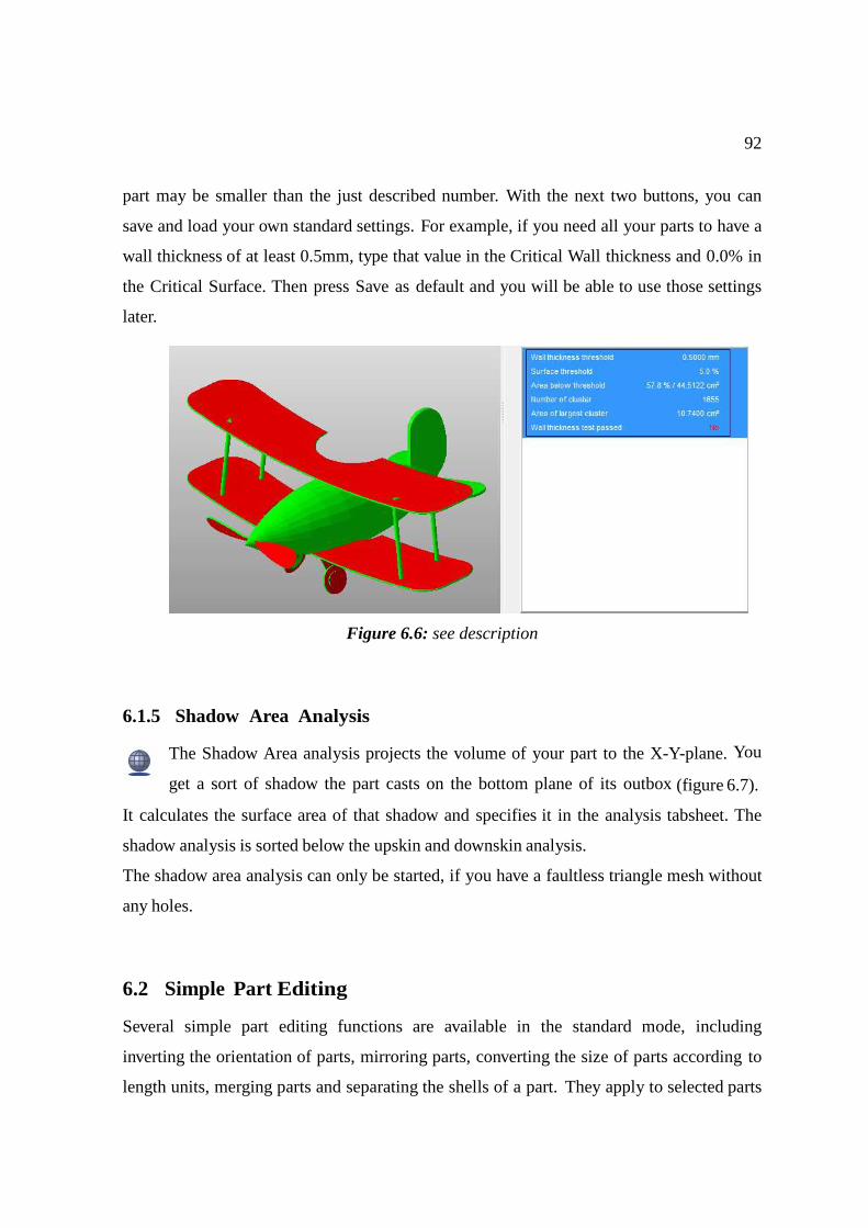
92
part may be smaller than the just described number. With the next two buttons, you can
save and load your own standard settings. For example, if you need all your parts to have a
wall thickness of at least 0.5mm, type that value in the Critical Wall thickness and 0.0% in
the Critical Surface. Then press Save as default and you will be able to use those settings
later.
Figure 6.6: see description
6.1.5 Shadow Area Analysis
The Shadow Area analysis projects the volume of your part to the X-Y-plane. You
get a sort of shadow the part casts on the bottom plane of its outbox (figure 6.7).
It calculates the surface area of that shadow and specifies it in the analysis tabsheet. The
shadow analysis is sorted below the upskin and downskin analysis.
The shadow area analysis can only be started, if you have a faultless triangle mesh without
any holes.
6.2 Simple Part Editing
Several simple part editing functions are available in the standard mode, including
inverting the orientation of parts, mirroring parts, converting the size of parts according to
length units, merging parts and separating the shells of a part. They apply to selected parts
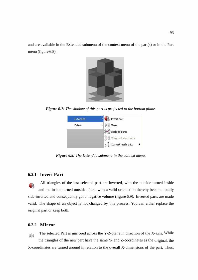
93
and are available in the Extended submenu of the context menu of the part(s) or in the Part
menu (figure 6.8).
Figure 6.7: The shadow of this part is projected to the bottom plane.
Figure 6.8: The Extended submenu in the context menu.
6.2.1 Invert Part
All triangles of the last selected part are inverted, with the outside turned inside
and the inside turned outside. Parts with a valid orientation thereby become totally
side-inverted and consequently get a negative volume (figure 6.9). Inverted parts are made
valid. The shape of an object is not changed by this process. You can either replace the
original part or keep both.
6.2.2 Mirror
The selected Part is mirrored across the Y-Z-plane in direction of the X-axis. While
the triangles of the new part have the same Y- and Z-coordinates as the original, the
X-coordinates are turned around in relation to the overall X-dimensions of the part. Thus,
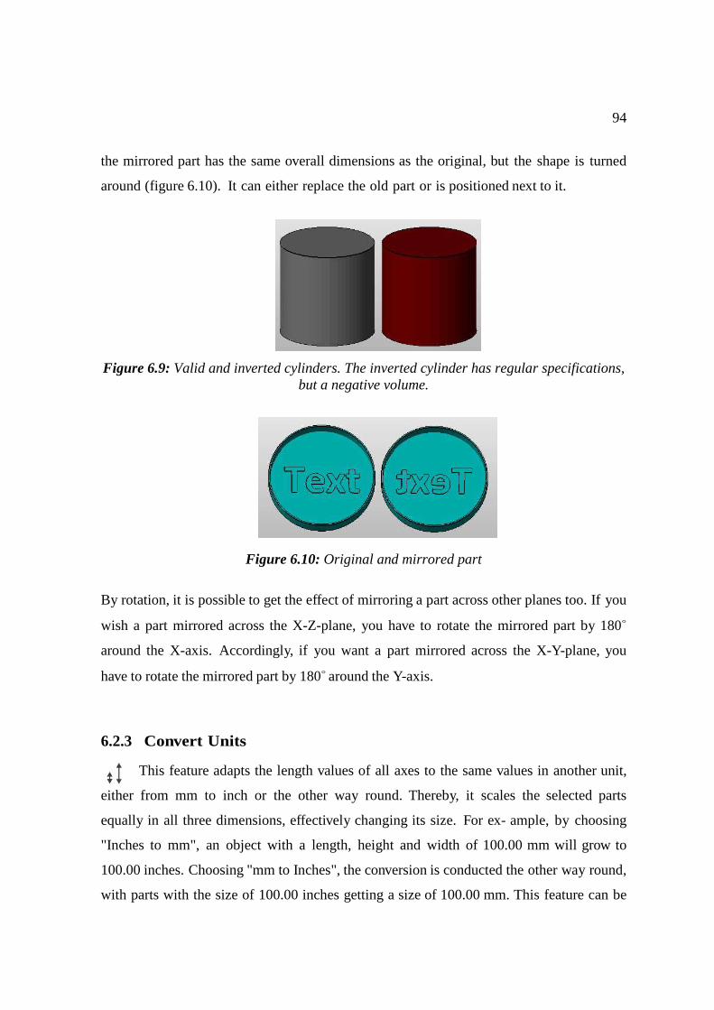
94
the mirrored part has the same overall dimensions as the original, but the shape is turned
around (figure 6.10). It can either replace the old part or is positioned next to it.
Figure 6.9: Valid and inverted cylinders. The inverted cylinder has regular specifications, but a negative volume.
Figure 6.10: Original and mirrored part
By rotation, it is possible to get the effect of mirroring a part across other planes too. If you
wish a part mirrored across the X-Z-plane, you have to rotate the mirrored part by 180◦
around the X-axis. Accordingly, if you want a part mirrored across the X-Y-plane, you
have to rotate the mirrored part by 180◦ around the Y-axis.
6.2.3 Convert Units
This feature adapts the length values of all axes to the same values in another unit,
either from mm to inch or the other way round. Thereby, it scales the selected parts
equally in all three dimensions, effectively changing its size. For ex- ample, by choosing
"Inches to mm", an object with a length, height and width of 100.00 mm will grow to
100.00 inches. Choosing "mm to Inches", the conversion is conducted the other way round,
with parts with the size of 100.00 inches getting a size of 100.00 mm. This feature can be
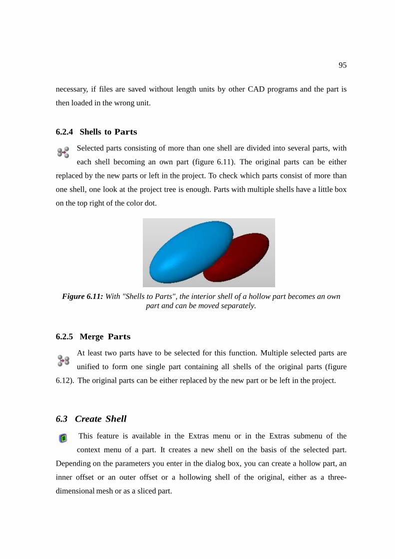
95
necessary, if files are saved without length units by other CAD programs and the part is
then loaded in the wrong unit.
6.2.4 Shells to Parts
Selected parts consisting of more than one shell are divided into several parts, with
each shell becoming an own part (figure 6.11). The original parts can be either
replaced by the new parts or left in the project. To check which parts consist of more than
one shell, one look at the project tree is enough. Parts with multiple shells have a little box
on the top right of the color dot.
Figure 6.11: With "Shells to Parts", the interior shell of a hollow part becomes an own part and can be moved separately.
6.2.5 Merge Parts
At least two parts have to be selected for this function. Multiple selected parts are
unified to form one single part containing all shells of the original parts (figure
6.12). The original parts can be either replaced by the new part or be left in the project.
6.3 Create Shell
This feature is available in the Extras menu or in the Extras submenu of the
context menu of a part. It creates a new shell on the basis of the selected part.
Depending on the parameters you enter in the dialog box, you can create a hollow part, an
inner offset or an outer offset or a hollowing shell of the original, either as a three-
dimensional mesh or as a sliced part.
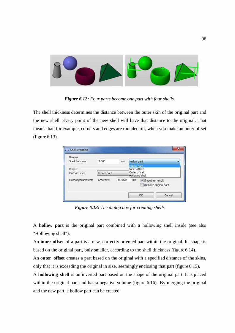
96
Figure 6.12: Four parts become one part with four shells.
The shell thickness determines the distance between the outer skin of the original part and
the new shell. Every point of the new shell will have that distance to the original. That
means that, for example, corners and edges are rounded off, when you make an outer offset
(figure 6.13).
Figure 6.13: The dialog box for creating shells
A hollow part is the original part combined with a hollowing shell inside (see also
"Hollowing shell").
An inner offset of a part is a new, correctly oriented part within the original. Its shape is
based on the original part, only smaller, according to the shell thickness (figure 6.14).
An outer offset creates a part based on the original with a specified distance of the skins,
only that it is exceeding the original in size, seemingly enclosing that part (figure 6.15).
A hollowing shell is an inverted part based on the shape of the original part. It is placed
within the original part and has a negative volume (figure 6.16). By merging the original
and the new part, a hollow part can be created.
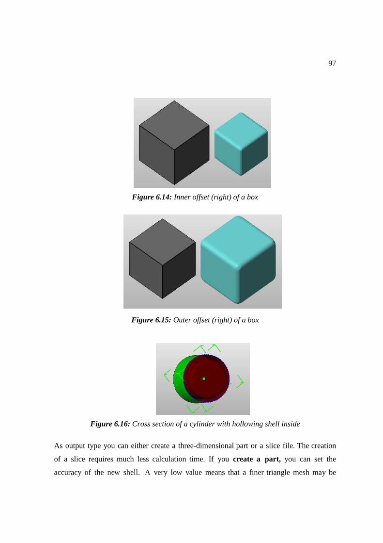
97
Figure 6.14: Inner offset (right) of a box
Figure 6.15: Outer offset (right) of a box
Figure 6.16: Cross section of a cylinder with hollowing shell inside
As output type you can either create a three-dimensional part or a slice file. The creation
of a slice requires much less calculation time. If you create a part, you can set the
accuracy of the new shell. A very low value means that a finer triangle mesh may be
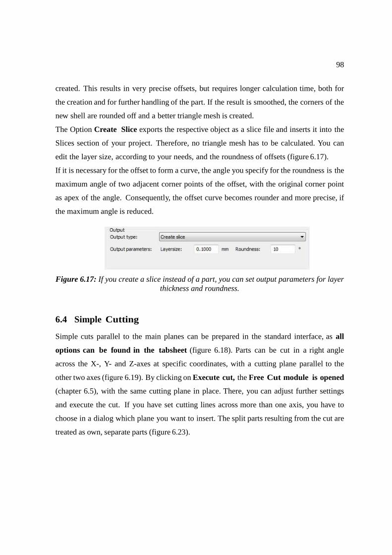
98
created. This results in very precise offsets, but requires longer calculation time, both for
the creation and for further handling of the part. If the result is smoothed, the corners of the
new shell are rounded off and a better triangle mesh is created.
The Option Create Slice exports the respective object as a slice file and inserts it into the
Slices section of your project. Therefore, no triangle mesh has to be calculated. You can
edit the layer size, according to your needs, and the roundness of offsets (figure 6.17).
If it is necessary for the offset to form a curve, the angle you specify for the roundness is the
maximum angle of two adjacent corner points of the offset, with the original corner point
as apex of the angle. Consequently, the offset curve becomes rounder and more precise, if
the maximum angle is reduced.
Figure 6.17: If you create a slice instead of a part, you can set output parameters for layer thickness and roundness.
6.4 Simple Cutting
Simple cuts parallel to the main planes can be prepared in the standard interface, as all
options can be found in the tabsheet (figure 6.18). Parts can be cut in a right angle
across the X-, Y- and Z-axes at specific coordinates, with a cutting plane parallel to the
other two axes (figure 6.19). By clicking on Execute cut, the Free Cut module is opened
(chapter 6.5), with the same cutting plane in place. There, you can adjust further settings
and execute the cut. If you have set cutting lines across more than one axis, you have to
choose in a dialog which plane you want to insert. The split parts resulting from the cut are
treated as own, separate parts (figure 6.23).
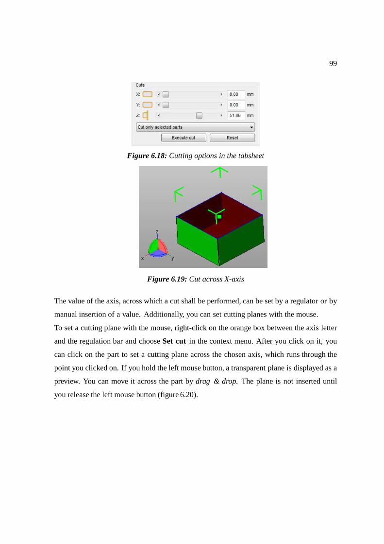
99
Figure 6.18: Cutting options in the tabsheet
Figure 6.19: Cut across X-axis
The value of the axis, across which a cut shall be performed, can be set by a regulator or by
manual insertion of a value. Additionally, you can set cutting planes with the mouse.
To set a cutting plane with the mouse, right-click on the orange box between the axis letter
and the regulation bar and choose Set cut in the context menu. After you click on it, you
can click on the part to set a cutting plane across the chosen axis, which runs through the
point you clicked on. If you hold the left mouse button, a transparent plane is displayed as a
preview. You can move it across the part by drag & drop. The plane is not inserted until
you release the left mouse button (figure 6.20).
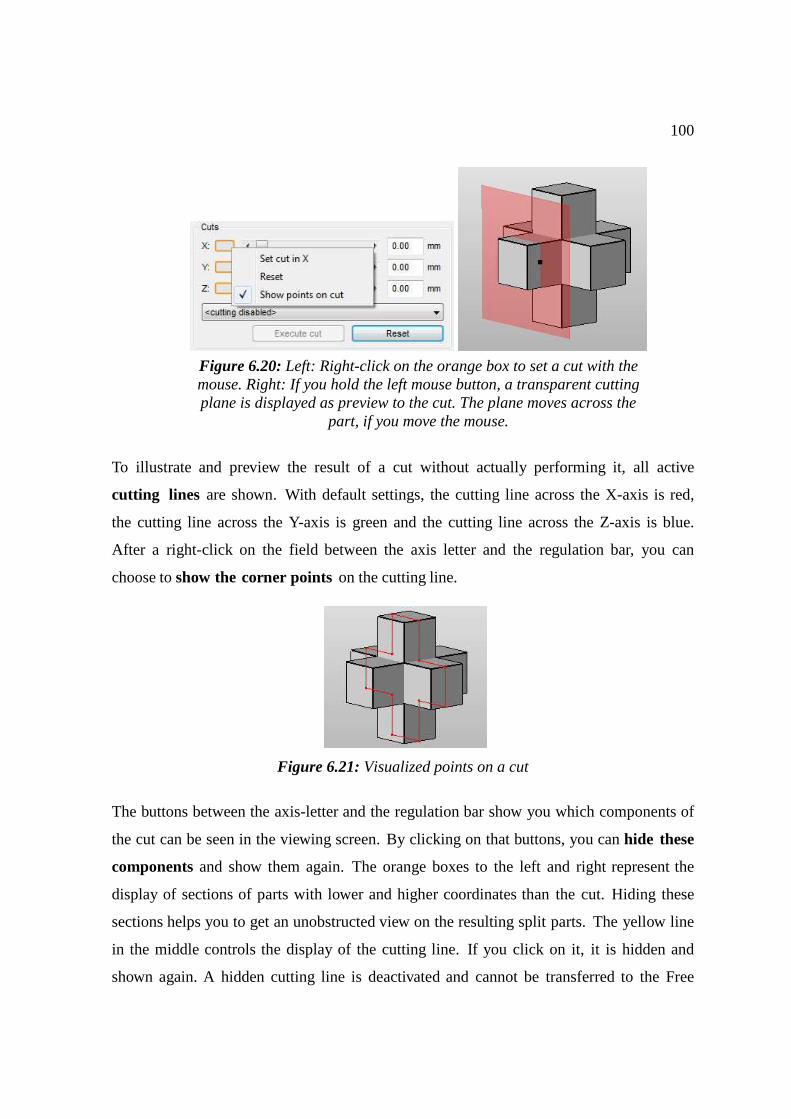
100
To illustrate and preview the result of a cut without actually performing it, all active
cutting lines are shown. With default settings, the cutting line across the X-axis is red,
the cutting line across the Y-axis is green and the cutting line across the Z-axis is blue.
After a right-click on the field between the axis letter and the regulation bar, you can
choose to show the corner points on the cutting line.
Figure 6.21: Visualized points on a cut
The buttons between the axis-letter and the regulation bar show you which components of
the cut can be seen in the viewing screen. By clicking on that buttons, you can hide these
components and show them again. The orange boxes to the left and right represent the
display of sections of parts with lower and higher coordinates than the cut. Hiding these
sections helps you to get an unobstructed view on the resulting split parts. The yellow line
in the middle controls the display of the cutting line. If you click on it, it is hidden and
shown again. A hidden cutting line is deactivated and cannot be transferred to the Free
Figure 6.20: Left: Right-click on the orange box to set a cut with the mouse. Right: If you hold the left mouse button, a transparent cutting plane is displayed as preview to the cut. The plane moves across the
part, if you move the mouse.
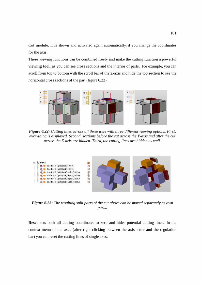
101
Cut module. It is shown and activated again automatically, if you change the coordinates
for the axis.
These viewing functions can be combined freely and make the cutting function a powerful
viewing tool, as you can see cross sections and the interior of parts. For example, you can
scroll from top to bottom with the scroll bar of the Z-axis and hide the top section to see the
horizontal cross sections of the part (figure 6.22).
Figure 6.22: Cutting lines across all three axes with three different viewing options. First, everything is displayed. Second, sections before the cut across the Y-axis and after the cut
across the Z-axis are hidden. Third, the cutting lines are hidden as well.
Figure 6.23: The resulting split parts of the cut above can be moved separately as own parts.
Reset sets back all cutting coordinates to zero and hides potential cutting lines. In the
context menu of the axes (after right-clicking between the axis letter and the regulation
bar) you can reset the cutting lines of single axes.
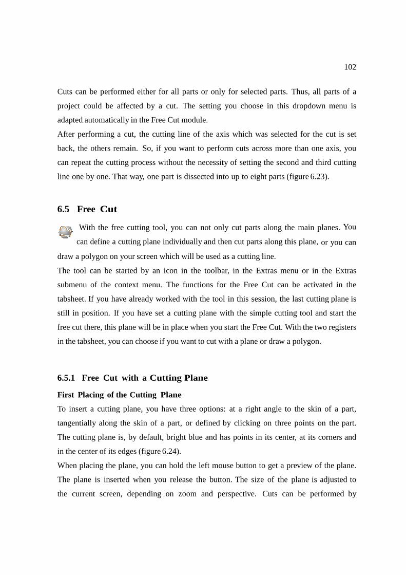
102
Cuts can be performed either for all parts or only for selected parts. Thus, all parts of a
project could be affected by a cut. The setting you choose in this dropdown menu is
adapted automatically in the Free Cut module.
After performing a cut, the cutting line of the axis which was selected for the cut is set
back, the others remain. So, if you want to perform cuts across more than one axis, you
can repeat the cutting process without the necessity of setting the second and third cutting
line one by one. That way, one part is dissected into up to eight parts (figure 6.23).
6.5 Free Cut
With the free cutting tool, you can not only cut parts along the main planes. You
can define a cutting plane individually and then cut parts along this plane, or you can
draw a polygon on your screen which will be used as a cutting line.
The tool can be started by an icon in the toolbar, in the Extras menu or in the Extras
submenu of the context menu. The functions for the Free Cut can be activated in the
tabsheet. If you have already worked with the tool in this session, the last cutting plane is
still in position. If you have set a cutting plane with the simple cutting tool and start the
free cut there, this plane will be in place when you start the Free Cut. With the two registers
in the tabsheet, you can choose if you want to cut with a plane or draw a polygon.
6.5.1 Free Cut with a Cutting Plane
First Placing of the Cutting Plane
To insert a cutting plane, you have three options: at a right angle to the skin of a part,
tangentially along the skin of a part, or defined by clicking on three points on the part.
The cutting plane is, by default, bright blue and has points in its center, at its corners and
in the center of its edges (figure 6.24).
When placing the plane, you can hold the left mouse button to get a preview of the plane.
The plane is inserted when you release the button. The size of the plane is adjusted to
the current screen, depending on zoom and perspective. Cuts can be performed by
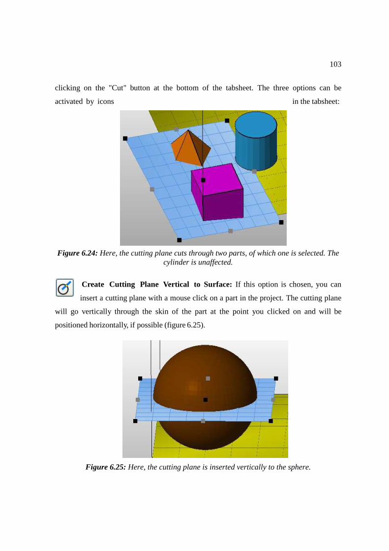
103
clicking on the "Cut" button at the bottom of the tabsheet. The three options can be
activated by icons in the tabsheet:
Figure 6.24: Here, the cutting plane cuts through two parts, of which one is selected. The cylinder is unaffected.
Create Cutting Plane Vertical to Surface: If this option is chosen, you can
insert a cutting plane with a mouse click on a part in the project. The cutting plane
will go vertically through the skin of the part at the point you clicked on and will be
positioned horizontally, if possible (figure 6.25).
Figure 6.25: Here, the cutting plane is inserted vertically to the sphere.
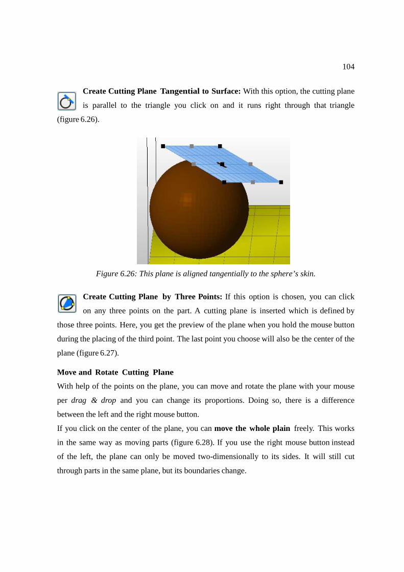
104
Create Cutting Plane Tangential to Surface: With this option, the cutting plane
is parallel to the triangle you click on and it runs right through that triangle
(figure 6.26).
Figure 6.26: This plane is aligned tangentially to the sphere’s skin.
Create Cutting Plane by Three Points: If this option is chosen, you can click
on any three points on the part. A cutting plane is inserted which is defined by
those three points. Here, you get the preview of the plane when you hold the mouse button
during the placing of the third point. The last point you choose will also be the center of the
plane (figure 6.27).
Move and Rotate Cutting Plane
With help of the points on the plane, you can move and rotate the plane with your mouse
per drag & drop and you can change its proportions. Doing so, there is a difference
between the left and the right mouse button.
If you click on the center of the plane, you can move the whole plain freely. This works
in the same way as moving parts (figure 6.28). If you use the right mouse button instead
of the left, the plane can only be moved two-dimensionally to its sides. It will still cut
through parts in the same plane, but its boundaries change.
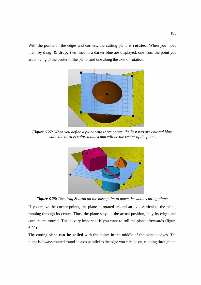
105
With the points on the edges and corners, the cutting plane is rotated. When you move
them by drag & drop, two lines in a darker blue are displayed, one from the point you
are moving to the center of the plane, and one along the axis of rotation.
Figure 6.27: When you define a plane with three points, the first two are colored blue, while the third is colored black and will be the center of the plane.
Figure 6.28: Use drag & drop on the base point to move the whole cutting plane.
If you move the corner points, the plane is rotated around an axis vertical to the plane,
running through its center. Thus, the plane stays in the actual position, only its edges and
corners are moved. This is very important if you want to roll the plane afterwards (figure
6.29).
The cutting plane can be rolled with the points in the middle of the plane’s edges. The
plane is always rotated round an axis parallel to the edge you clicked on, running through the
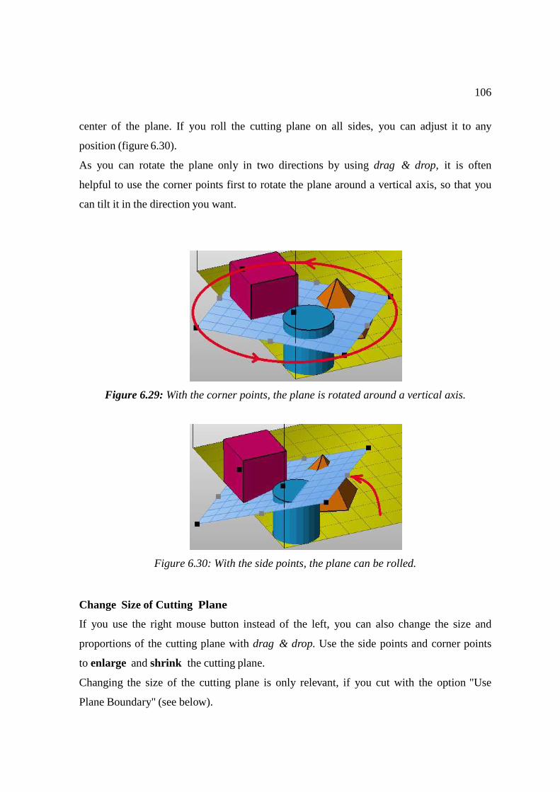
106
center of the plane. If you roll the cutting plane on all sides, you can adjust it to any
position (figure 6.30).
As you can rotate the plane only in two directions by using drag & drop, it is often
helpful to use the corner points first to rotate the plane around a vertical axis, so that you
can tilt it in the direction you want.
Figure 6.29: With the corner points, the plane is rotated around a vertical axis.
Figure 6.30: With the side points, the plane can be rolled.
Change Size of Cutting Plane
If you use the right mouse button instead of the left, you can also change the size and
proportions of the cutting plane with drag & drop. Use the side points and corner points
to enlarge and shrink the cutting plane.
Changing the size of the cutting plane is only relevant, if you cut with the option "Use
Plane Boundary" (see below).
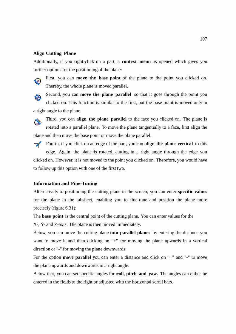
107
Align Cutting Plane
Additionally, if you right-click on a part, a context menu is opened which gives you
further options for the positioning of the plane:
First, you can move the base point of the plane to the point you clicked on.
Thereby, the whole plane is moved parallel.
Second, you can move the plane parallel so that it goes through the point you
clicked on. This function is similar to the first, but the base point is moved only in
a right angle to the plane.
Third, you can align the plane parallel to the face you clicked on. The plane is
rotated into a parallel plane. To move the plane tangentially to a face, first align the
plane and then move the base point or move the plane parallel.
Fourth, if you click on an edge of the part, you can align the plane vertical to this
edge. Again, the plane is rotated, cutting in a right angle through the edge you
clicked on. However, it is not moved to the point you clicked on. Therefore, you would have
to follow up this option with one of the first two. Information and Fine-Tuning
Alternatively to positioning the cutting plane in the screen, you can enter specific values
for the plane in the tabsheet, enabling you to fine-tune and position the plane more
precisely (figure 6.31):
The base point is the central point of the cutting plane. You can enter values for the
X-, Y- and Z-axis. The plane is then moved immediately.
Below, you can move the cutting plane into parallel planes by entering the distance you
want to move it and then clicking on "+" for moving the plane upwards in a vertical
direction or "-" for moving the plane downwards.
For the option move parallel you can enter a distance and click on "+" and "-" to move
the plane upwards and downwards in a right angle.
Below that, you can set specific angles for roll, pitch and yaw. The angles can either be
entered in the fields to the right or adjusted with the horizontal scroll bars.
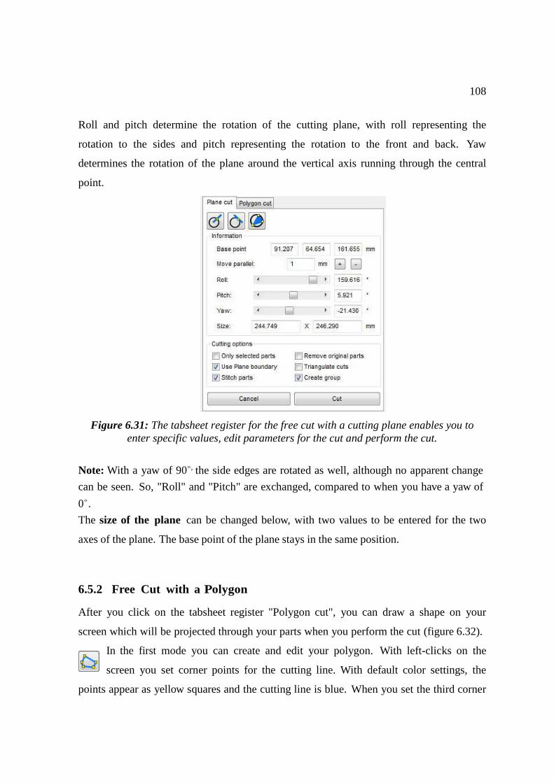
108
Roll and pitch determine the rotation of the cutting plane, with roll representing the
rotation to the sides and pitch representing the rotation to the front and back. Yaw
determines the rotation of the plane around the vertical axis running through the central
point.
Figure 6.31: The tabsheet register for the free cut with a cutting plane enables you to enter specific values, edit parameters for the cut and perform the cut.
Note: With a yaw of 90◦, the side edges are rotated as well, although no apparent change
can be seen. So, "Roll" and "Pitch" are exchanged, compared to when you have a yaw of
0◦.
The size of the plane can be changed below, with two values to be entered for the two
axes of the plane. The base point of the plane stays in the same position.
6.5.2 Free Cut with a Polygon
After you click on the tabsheet register "Polygon cut", you can draw a shape on your
screen which will be projected through your parts when you perform the cut (figure 6.32).
In the first mode you can create and edit your polygon. With left-clicks on the
screen you set corner points for the cutting line. With default color settings, the
points appear as yellow squares and the cutting line is blue. When you set the third corner
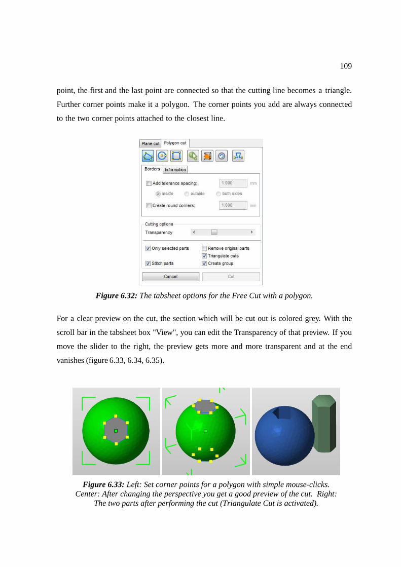
109
point, the first and the last point are connected so that the cutting line becomes a triangle.
Further corner points make it a polygon. The corner points you add are always connected
to the two corner points attached to the closest line.
Figure 6.32: The tabsheet options for the Free Cut with a polygon.
For a clear preview on the cut, the section which will be cut out is colored grey. With the
scroll bar in the tabsheet box "View", you can edit the Transparency of that preview. If you
move the slider to the right, the preview gets more and more transparent and at the end
vanishes (figure 6.33, 6.34, 6.35).
Figure 6.33: Left: Set corner points for a polygon with simple mouse-clicks. Center: After changing the perspective you get a good preview of the cut. Right:
The two parts after performing the cut (Triangulate Cut is activated).
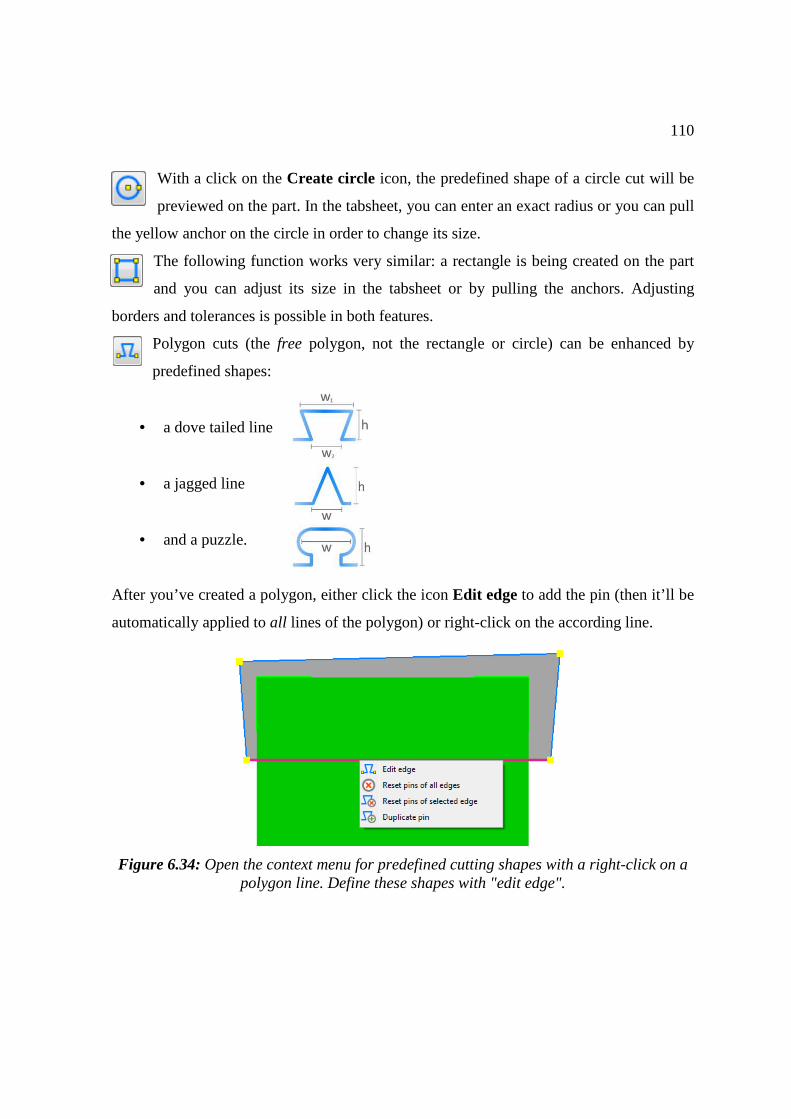
110
With a click on the Create circle icon, the predefined shape of a circle cut will be
previewed on the part. In the tabsheet, you can enter an exact radius or you can pull
the yellow anchor on the circle in order to change its size.
The following function works very similar: a rectangle is being created on the part
and you can adjust its size in the tabsheet or by pulling the anchors. Adjusting
borders and tolerances is possible in both features.
Polygon cuts (the free polygon, not the rectangle or circle) can be enhanced by
predefined shapes:
• a dove tailed line
• a jagged line
• and a puzzle.
After you’ve created a polygon, either click the icon Edit edge to add the pin (then it’ll be
automatically applied to all lines of the polygon) or right-click on the according line.
Figure 6.34: Open the context menu for predefined cutting shapes with a right-click on a polygon line. Define these shapes with "edit edge".
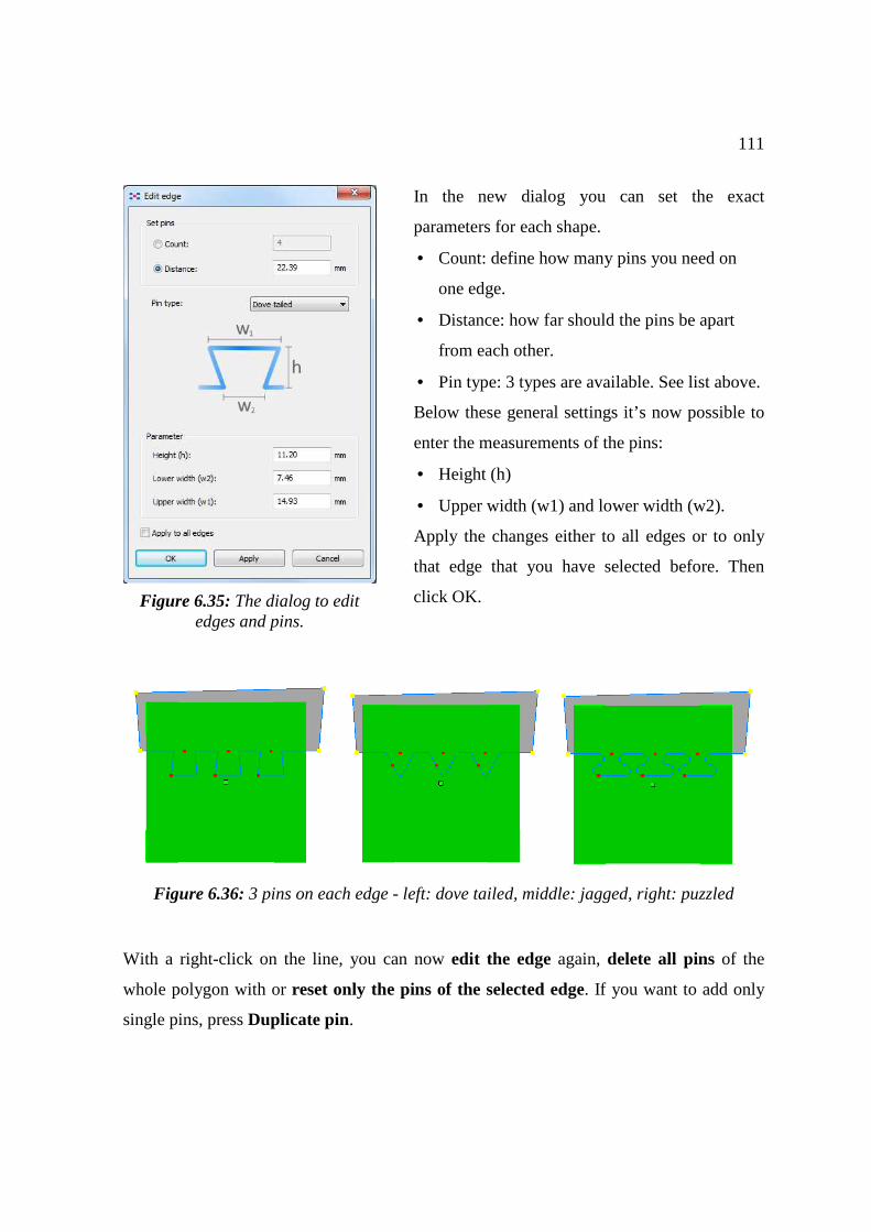
111
In the new dialog you can set the exact
parameters for each shape.
• Count: define how many pins you need on
one edge.
• Distance: how far should the pins be apart
from each other.
• Pin type: 3 types are available. See list above.
Below these general settings it’s now possible to
enter the measurements of the pins:
• Height (h)
• Upper width (w1) and lower width (w2).
Apply the changes either to all edges or to only
that edge that you have selected before. Then
click OK.
Figure 6.36: 3 pins on each edge - left: dove tailed, middle: jagged, right: puzzled
With a right-click on the line, you can now edit the edge again, delete all pins of the
whole polygon with or reset only the pins of the selected edge. If you want to add only
single pins, press Duplicate pin.
Figure 6.35: The dialog to edit edges and pins.
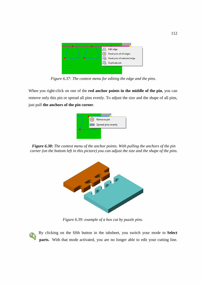
112
When you right-click on one of the red anchor points in the middle of the pin, you can
remove only this pin or spread all pins evenly. To adjust the size and the shape of all pins,
just pull the anchors of the pin corner.
By clicking on the fifth button in the tabsheet, you switch your mode to Select
parts. With that mode activated, you are no longer able to edit your cutting line.
Figure 6.37: The context menu for editing the edge and the pins.
Figure 6.38: The context menu of the anchor points. With pulling the anchors of the pin corner (on the bottom left in this picture) you can adjust the size and the shape of the pins.
Figure 6.39: example of a box cut by puzzle pins.
113
Instead, all options of the standard interface become available. You select parts by clicking
on them and you can move and rotate them by drag & drop. Also, all context menus of the
standard interface are available.
If you change the perspective after setting the first corner points, you can look at the
cutting section from different angles. The cutting line is not rotated with the
perspective. With the button Reset perspective to cutting direction you can set the
perspective back to the one you had when you started setting cutting points.
To change the shape of the cutting line, you can move the points by drag & drop. The
points are always moved sideways and never up and down (as the cutting line is projected
through the whole area where it meets parts anyway). So, when you have changed the
perspective, the shift can be a bit different to what you would expect intuitively. Rotate the
perspective with the right mouse button to understand how the cutting line has been
changed. After right-clicking on a corner point of the polygon, you can remove that point
in the context menu.
When you click on Cut, the cutting line is projected through your parts. Everything within
that projection is then cut out of your parts. The direction of the projection corresponds to
the perspective from which you were looking at the project when you started drawing the
line (figure 6.33, 6.34). You automatically leave the Free Cut module.
With Reset in the tabsheet you can remove your polygon and start a new line. You
automatically get back into the mode "Create/Edit polygon".
In the borders tab below (figure 6.36), you can add tolerance spacing to the cut. This
means that additional space between the two resulting cuts will also be cut off, which gives
clearance to the parts. If you use a 3D printing technology, where the contours swell up at
little, this is very helpful.
Activate the tolerance spacing with a check mark first, then define its thickness. You can
choose if you want the space to be added inside, outside or on both sides of the original
cutting line.
With a check mark on create round corners, the corners of the polygon will be
smoothed. The value next to it defines the radius of this rounding.
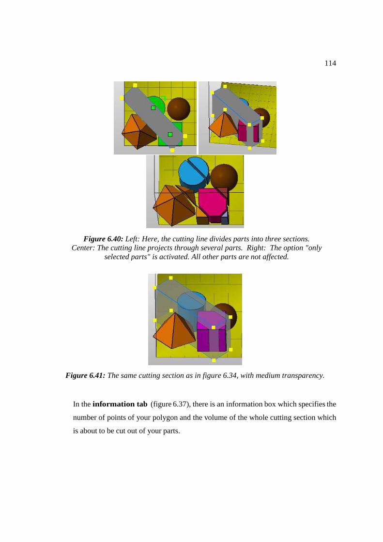
114
Figure 6.41: The same cutting section as in figure 6.34, with medium transparency.
In the information tab (figure 6.37), there is an information box which specifies the
number of points of your polygon and the volume of the whole cutting section which
is about to be cut out of your parts.
Figure 6.40: Left: Here, the cutting line divides parts into three sections. Center: The cutting line projects through several parts. Right: The option "only
selected parts" is activated. All other parts are not affected.
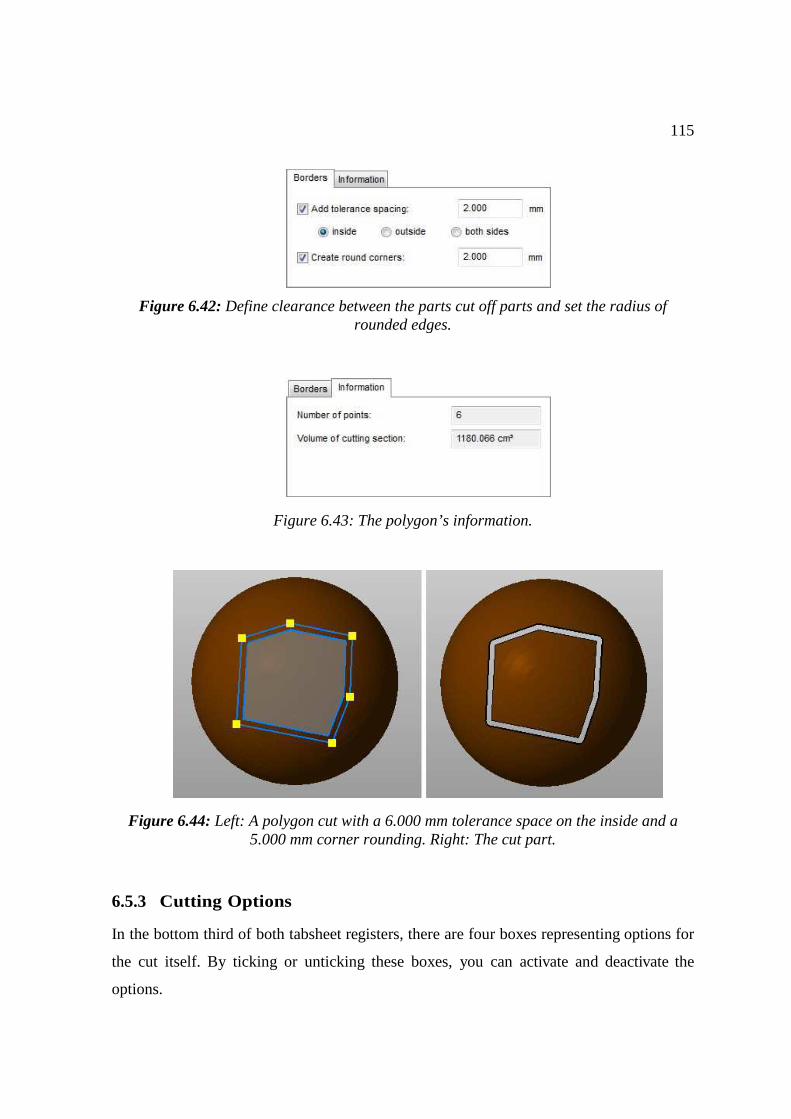
115
Figure 6.42: Define clearance between the parts cut off parts and set the radius of rounded edges.
Figure 6.43: The polygon’s information.
Figure 6.44: Left: A polygon cut with a 6.000 mm tolerance space on the inside and a
5.000 mm corner rounding. Right: The cut part.
6.5.3 Cutting Options
In the bottom third of both tabsheet registers, there are four boxes representing options for
the cut itself. By ticking or unticking these boxes, you can activate and deactivate the
options.

116
You can cut only selected parts or all parts, through which the cutting plane or line runs.
Selection options are the same as in the standard module.
When you use the plane boundary, the cut is only conducted as far as the outer edges
of the plane go. If the box is not ticked, the parts are cut completely through along the
plane, independently from the size of the displayed cutting plane. This option can only be
chosen for cuts with a cutting plane.
If you Stitch parts, open triangle edges are connected. Sometimes, if the option
"Triangulate Cut" (see below) is activated, the cutting tool produces open edges (for
example if a part has self-intersections) which can be connected with this additional step.
Next, you can choose to Remove the original parts and replace them by the cut parts. If
you do not remove them, they are hidden after the cut.
If you triangulate the cut, holes that emerge at the new cut parts are closed automatically
with a straight surface across the cut. If not, the parts will be open (figure 6.39).
Figure 6.45: Non-triangulated (left) and triangulated (right) cut of a box.
With the option Create group, the cut parts are moved into a new group in the project tree.
Finally, at the bottom of the tabsheet, you can either Cut to perform the cutting with the
chosen plane and settings. The cut parts are then inserted into a group in the project tree.
You can also cancel the cutting and leave the cutting tool without doing anything. You can
go back to the tool any time. The cutting plane remains in place.
117
6.6 Boolean Operations
The Boolean operations module creates either a unification or a cross section of two
or more overlapping parts, or subtracts one overlapping part from the other,
effectively cutting the cross section out of the remaining part. They can only be performed
with closed and oriented volume meshes and will always result in new parts.
To conduct Boolean operations, first move parts together so that they overlap, then select
all parts you want to use. Start the Boolean Operations module in the toolbar, in the Extras
menu or in the Extras submenu of the context menu. This opens a new screen and options
for Boolean operations in the tabsheet. The screen includes only the selected parts.
In the tabsheet (figure 6.40), the parts are listed in two fields. Parts which shall remain
after the Boolean operation are marked green in the screen and are listed in the left field.
Parts that shall be subtracted from the resulting part of the Boolean operation are marked
red and listed in the right field.
This basic setting for a part is changed either by clicking on the part in the screen or by
selecting the part in the tabsheet and clicking on the arrow below the field. The color of
the part will be changed and it will be moved into the other parts field in the tabsheet.
The Log field in the tabsheet shows the result of a test, if the parts prepared for Boolean
operations are closed and oriented. The test is conducted every time you start the Boolean
Operations module. If one of the selected parts fails this test, no Boolean operations can
be conducted.
Depending on how you have assigned your parts, three major Boolean operations can be
conducted, based on position and volume of the different parts: Parts can be unified, an
intersection of parts can be created and parts can be subtracted from one another.
Thereby, the triangle meshes of the parts are retriangulated, resulting in new, closed and
oriented volume triangle meshes. The operations are available in the "Actions" section at
the bottom of the tabsheet and in the context menu by right-clicking on the screen.
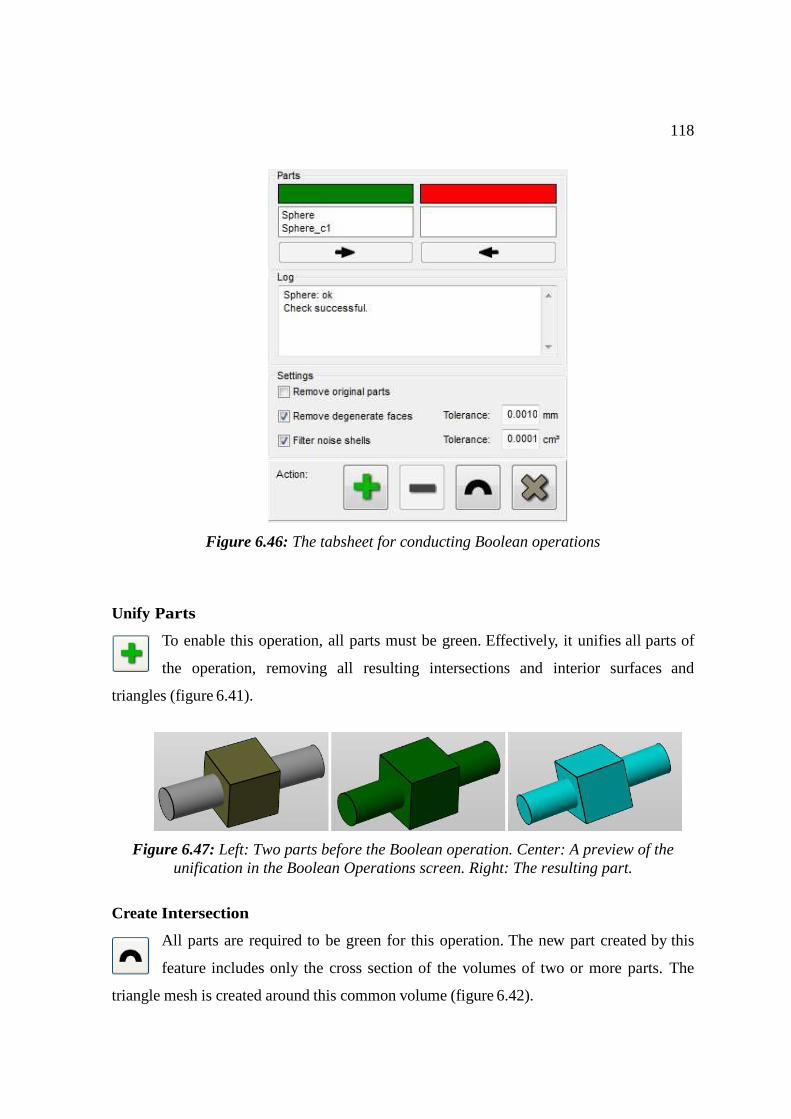
118
Figure 6.46: The tabsheet for conducting Boolean operations
Unify Parts
To enable this operation, all parts must be green. Effectively, it unifies all parts of
the operation, removing all resulting intersections and interior surfaces and
triangles (figure 6.41).
Figure 6.47: Left: Two parts before the Boolean operation. Center: A preview of the unification in the Boolean Operations screen. Right: The resulting part.
Create Intersection
All parts are required to be green for this operation. The new part created by this
feature includes only the cross section of the volumes of two or more parts. The
triangle mesh is created around this common volume (figure 6.42).
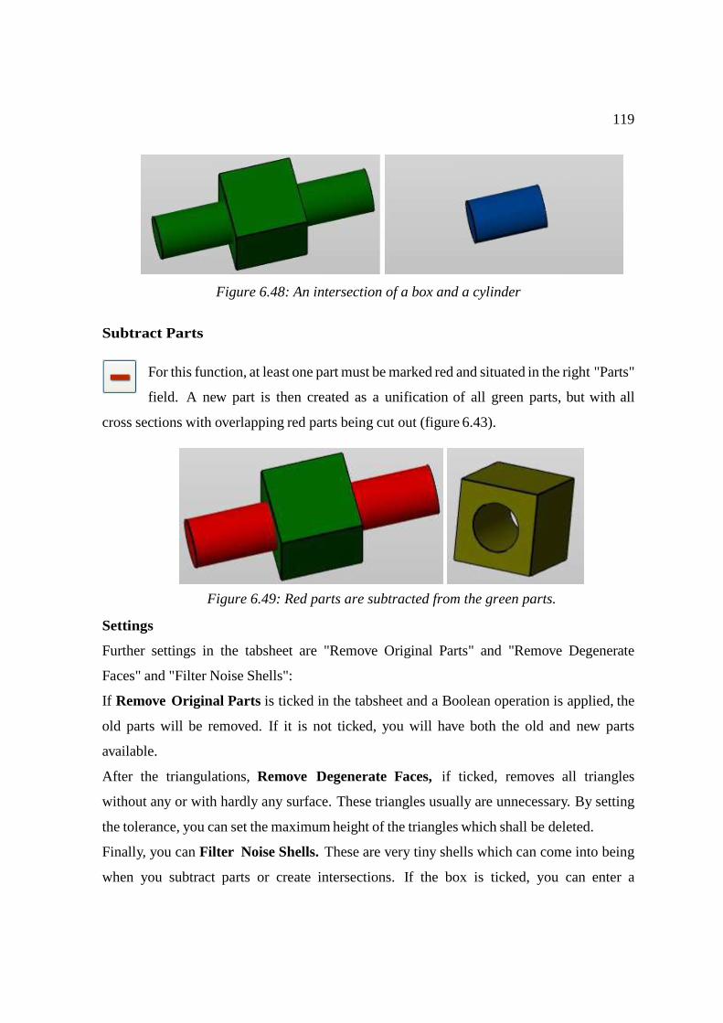
119
Figure 6.48: An intersection of a box and a cylinder
Subtract Parts
For this function, at least one part must be marked red and situated in the right "Parts"
field. A new part is then created as a unification of all green parts, but with all
cross sections with overlapping red parts being cut out (figure 6.43).
Settings
Further settings in the tabsheet are "Remove Original Parts" and "Remove Degenerate
Faces" and "Filter Noise Shells":
If Remove Original Parts is ticked in the tabsheet and a Boolean operation is applied, the
old parts will be removed. If it is not ticked, you will have both the old and new parts
available.
After the triangulations, Remove Degenerate Faces, if ticked, removes all triangles
without any or with hardly any surface. These triangles usually are unnecessary. By setting
the tolerance, you can set the maximum height of the triangles which shall be deleted.
Finally, you can Filter Noise Shells. These are very tiny shells which can come into being
when you subtract parts or create intersections. If the box is ticked, you can enter a
Figure 6.49: Red parts are subtracted from the green parts.
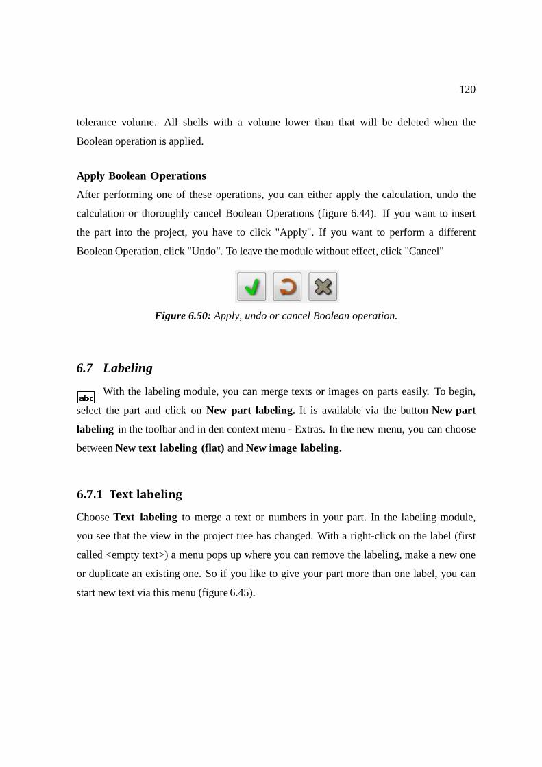
120
tolerance volume. All shells with a volume lower than that will be deleted when the
Boolean operation is applied. Apply Boolean Operations
After performing one of these operations, you can either apply the calculation, undo the
calculation or thoroughly cancel Boolean Operations (figure 6.44). If you want to insert
the part into the project, you have to click "Apply". If you want to perform a different
Boolean Operation, click "Undo". To leave the module without effect, click "Cancel"
Figure 6.50: Apply, undo or cancel Boolean operation.
6.7 Labeling
With the labeling module, you can merge texts or images on parts easily. To begin,
select the part and click on New part labeling. It is available via the button New part
labeling in the toolbar and in den context menu - Extras. In the new menu, you can choose
between New text labeling (flat) and New image labeling.
6.7.1 Text labeling
Choose Text labeling to merge a text or numbers in your part. In the labeling module,
you see that the view in the project tree has changed. With a right-click on the label (first
called <empty text>) a menu pops up where you can remove the labeling, make a new one
or duplicate an existing one. So if you like to give your part more than one label, you can
start new text via this menu (figure 6.45).
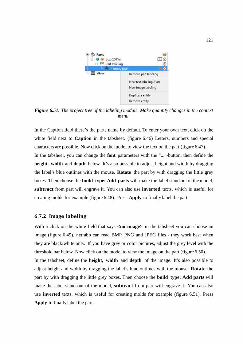
121
Figure 6.51: The project tree of the labeling module. Make quantity changes in the context menu.
In the Caption field there’s the parts name by default. To enter your own text, click on the
white field next to Caption in the tabsheet. (figure 6.46) Letters, numbers and special
characters are possible. Now click on the model to view the text on the part (figure 6.47).
In the tabsheet, you can change the font parameters with the "..."-button, then define the
height, width and depth below. It’s also possible to adjust height and width by dragging
the label’s blue outlines with the mouse. Rotate the part by with dragging the little grey
boxes. Then choose the build type: Add parts will make the label stand out of the model,
subtract from part will engrave it. You can also use inverted texts, which is useful for
creating molds for example (figure 6.48). Press Apply to finally label the part.
6.7.2 Image labeling
With a click on the white field that says <no image> in the tabsheet you can choose an
image (figure 6.49). netfabb can read BMP, PNG and JPEG files - they work best when
they are black/white only. If you have grey or color pictures, adjust the grey level with the
threshold bar below. Now click on the model to view the image on the part (figure 6.50).
In the tabsheet, define the height, width and depth of the image. It’s also possible to
adjust height and width by dragging the label’s blue outlines with the mouse. Rotate the
part by with dragging the little grey boxes. Then choose the build type: Add parts will
make the label stand out of the model, subtract from part will engrave it. You can also
use inverted texts, which is useful for creating molds for example (figure 6.51). Press
Apply to finally label the part.
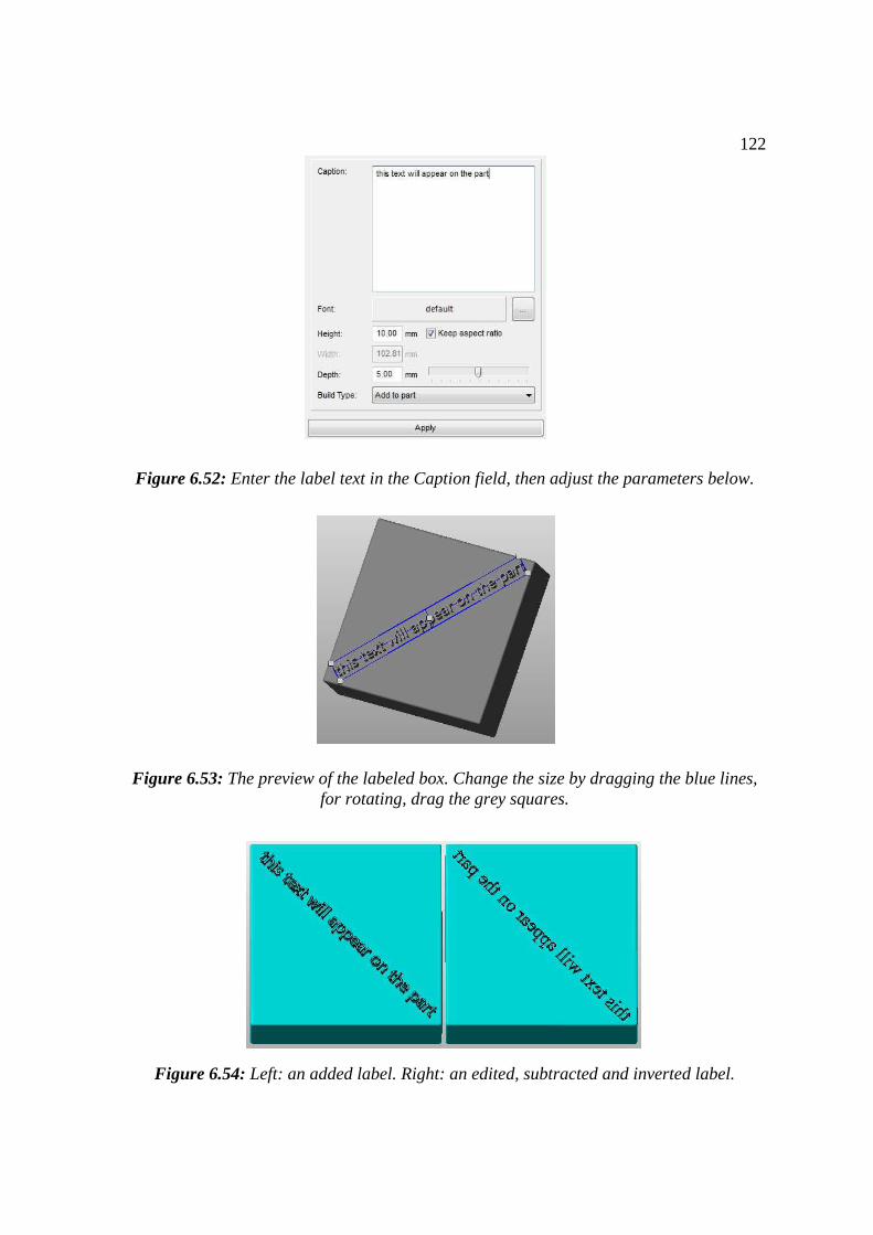
122
Figure 6.52: Enter the label text in the Caption field, then adjust the parameters below.
Figure 6.53: The preview of the labeled box. Change the size by dragging the blue lines, for rotating, drag the grey squares.
Figure 6.54: Left: an added label. Right: an edited, subtracted and inverted label.
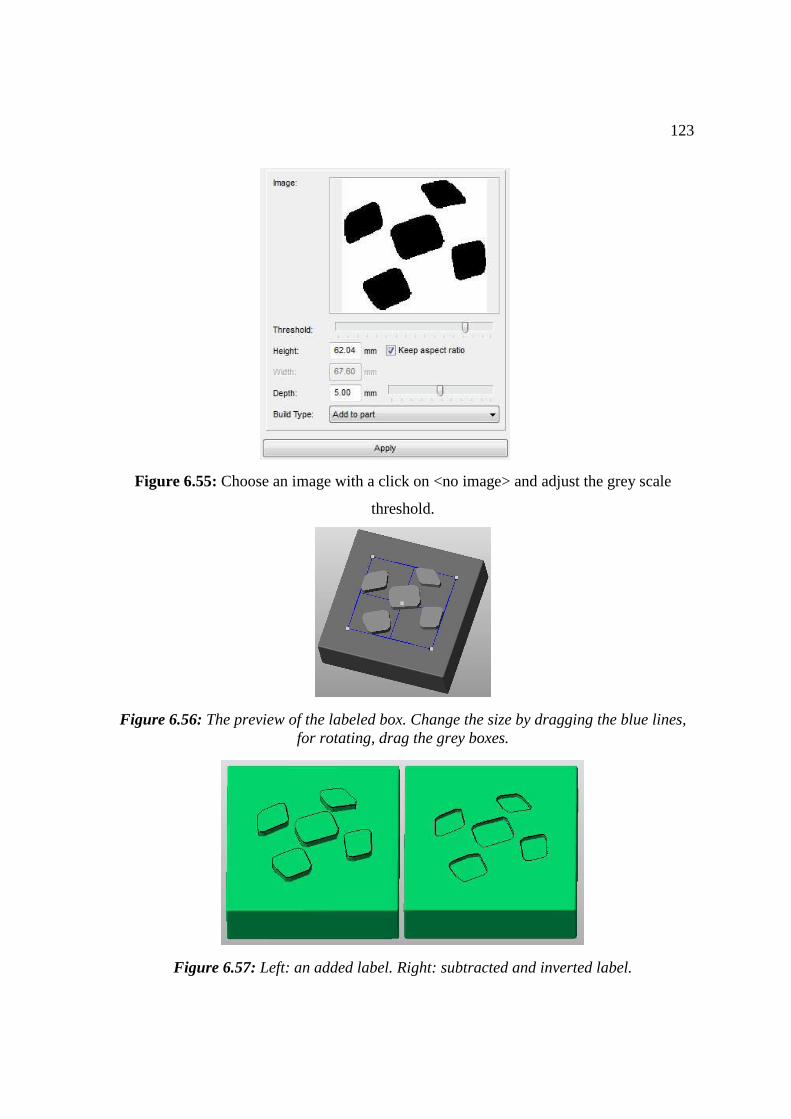
123
Figure 6.55: Choose an image with a click on <no image> and adjust the grey scale
threshold.
Figure 6.56: The preview of the labeled box. Change the size by dragging the blue lines, for rotating, drag the grey boxes.
Figure 6.57: Left: an added label. Right: subtracted and inverted label.
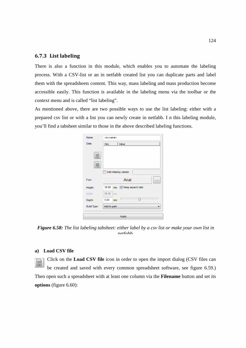
124
6.7.3 List labeling
There is also a function in this module, which enables you to automate the labeling
process. With a CSV-list or an in netfabb created list you can duplicate parts and label
them with the spreadsheets content. This way, mass labeling and mass production become
accessible easily. This function is available in the labeling menu via the toolbar or the
context menu and is called “list labeling”.
As mentioned above, there are two possible ways to use the list labeling: either with a
prepared csv list or with a list you can newly create in netfabb. I n this labeling module,
you’ll find a tabsheet similar to those in the above described labeling functions.
a) Load CSV file
Click on the Load CSV file icon in order to open the import dialog (CSV files can
be created and saved with every common spreadsheet software, see figure 6.59.)
Then open such a spreadsheet with at least one column via the Filename button and set its
options (figure 6.60):
Figure 6.58: The list labeling tabsheet: either label by a csv list or make your own list in netfabb.
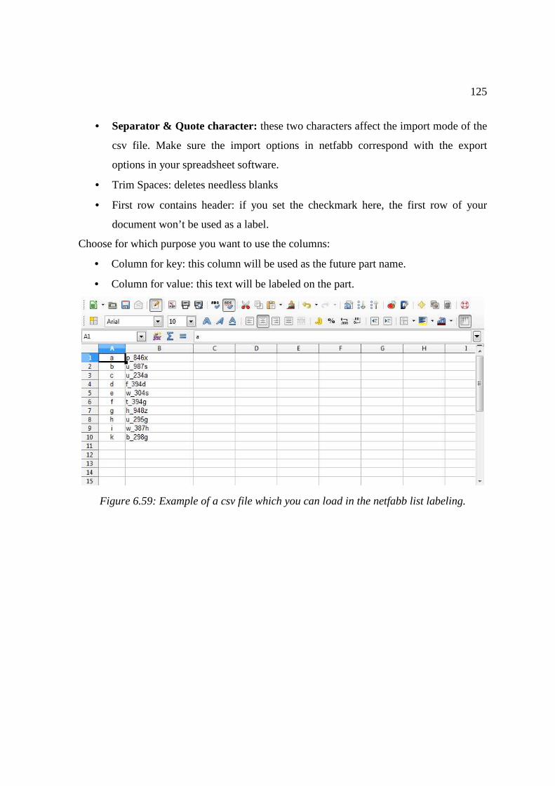
125
• Separator & Quote character: these two characters affect the import mode of the
csv file. Make sure the import options in netfabb correspond with the export
options in your spreadsheet software.
• Trim Spaces: deletes needless blanks
• First row contains header: if you set the checkmark here, the first row of your
document won’t be used as a label.
Choose for which purpose you want to use the columns:
• Column for key: this column will be used as the future part name.
• Column for value: this text will be labeled on the part.
Figure 6.59: Example of a csv file which you can load in the netfabb list labeling.
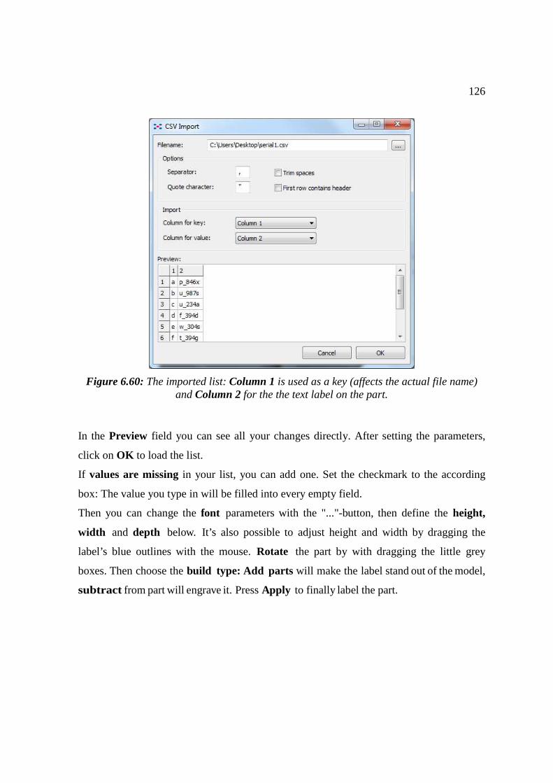
126
Figure 6.60: The imported list: Column 1 is used as a key (affects the actual file name) and Column 2 for the the text label on the part.
In the Preview field you can see all your changes directly. After setting the parameters,
click on OK to load the list.
If values are missing in your list, you can add one. Set the checkmark to the according
box: The value you type in will be filled into every empty field.
Then you can change the font parameters with the "..."-button, then define the height,
width and depth below. It’s also possible to adjust height and width by dragging the
label’s blue outlines with the mouse. Rotate the part by with dragging the little grey
boxes. Then choose the build type: Add parts will make the label stand out of the model,
subtract from part will engrave it. Press Apply to finally label the part.

127
Figure 6.61: Result of a list labeling process with a csv file.
b) Generate a new list in netfabb
If you don’t have a prepared csv list, then you can create a new list easily in netfabb.
Click on the according icon in the tabsheet in order to get into the dialog for
generating a numbered list (figure 6.62). Then set the following parameters:
• Prefix: tag at the beginning of each label
• Suffix: tag at the end of each label
• Start: first value that will be labeled
• Count: determines how many parts you will have in the end
• Step: values will be left out, e.g. 1 = 1, 2, 3; 2 = 1, 3, 5; 3 = 1, 4, 7
• Digits: digits displayed between pre- and suffix, e.g. 1 = 1; 2 = 01; 3 = 001
• Example: Shows the preview of the new list
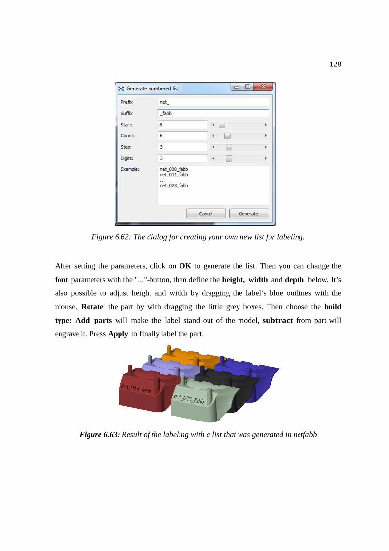
128
Figure 6.62: The dialog for creating your own new list for labeling.
After setting the parameters, click on OK to generate the list. Then you can change the
font parameters with the "..."-button, then define the height, width and depth below. It’s
also possible to adjust height and width by dragging the label’s blue outlines with the
mouse. Rotate the part by with dragging the little grey boxes. Then choose the build
type: Add parts will make the label stand out of the model, subtract from part will
engrave it. Press Apply to finally label the part.
Figure 6.63: Result of the labeling with a list that was generated in netfabb
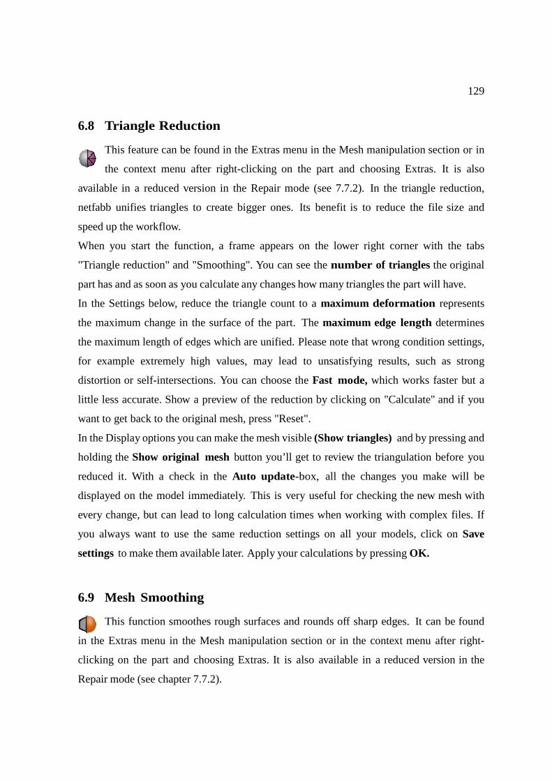
129
6.8 Triangle Reduction
This feature can be found in the Extras menu in the Mesh manipulation section or in
the context menu after right-clicking on the part and choosing Extras. It is also
available in a reduced version in the Repair mode (see 7.7.2). In the triangle reduction,
netfabb unifies triangles to create bigger ones. Its benefit is to reduce the file size and
speed up the workflow.
When you start the function, a frame appears on the lower right corner with the tabs
"Triangle reduction" and "Smoothing". You can see the number of triangles the original
part has and as soon as you calculate any changes how many triangles the part will have.
In the Settings below, reduce the triangle count to a maximum deformation represents
the maximum change in the surface of the part. The maximum edge length determines
the maximum length of edges which are unified. Please note that wrong condition settings,
for example extremely high values, may lead to unsatisfying results, such as strong
distortion or self-intersections. You can choose the Fast mode, which works faster but a
little less accurate. Show a preview of the reduction by clicking on "Calculate" and if you
want to get back to the original mesh, press "Reset".
In the Display options you can make the mesh visible (Show triangles) and by pressing and
holding the Show original mesh button you’ll get to review the triangulation before you
reduced it. With a check in the Auto update-box, all the changes you make will be
displayed on the model immediately. This is very useful for checking the new mesh with
every change, but can lead to long calculation times when working with complex files. If
you always want to use the same reduction settings on all your models, click on Save
settings to make them available later. Apply your calculations by pressing OK.
6.9 Mesh Smoothing
This function smoothes rough surfaces and rounds off sharp edges. It can be found
in the Extras menu in the Mesh manipulation section or in the context menu after right-
clicking on the part and choosing Extras. It is also available in a reduced version in the
Repair mode (see chapter 7.7.2).
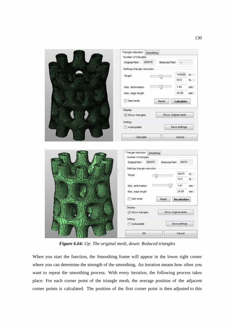
130
Figure 6.64: Up: The original mesh, down: Reduced triangles
When you start the function, the Smoothing frame will appear in the lower right corner
where you can determine the strength of the smoothing. An iteration means how often you
want to repeat the smoothing process. With every iteration, the following process takes
place: For each corner point of the triangle mesh, the average position of the adjacent
corner points is calculated. The position of the first corner point is then adjusted to this

131
average value. That way, surfaces become smoother and corners and sharp edges of objects
become rounder and are pulled inwards.
Prevent shrinking: The part will be deformed but the volume won’t get any smaller.
Independent of triangulation: The smoothing doesn’t happen on the basis of the
triangle mesh but of the actual part shape. This way, you hardly get any deformation effect.
Striking edges will be retained, less rough surfaces will be smoothed. To have a more
regular triangle mesh and improve smoothing, you can refine the mesh and reduce the
max. edge length. Show a preview of the smoothing by clicking on "Calculate" and if you
want to get back to the original mesh, press "Reset".
In the Display options you can make the mesh visible (Show triangles) and by pressing and
holding the Show original mesh button you’ll get to review the triangulation before you
smoothed it. With a check in the Auto update-box, all the changes you make will be
displayed on the model immediately. This is very useful for checking the new mesh with
every change, but can lead to long calculation times when working with complex files. If
you always want to use the same reduction settings on all your models, click on Save
settings to make them available later. Apply your calculations by pressing OK.
6.10 Remesh
If your part has a very irregular mesh, you can remesh the triangles and get a
smoother shape. This is very helpful for scans and organic shapes. The feature is
available in the Extras Menu in the Mesh manipulation section. First, choose the
resolution the new mesh should have (figure 6.54). The lower this value is, the more similar
the result will be to the existing part and the finer the triangle mesh will be. As the value
becomes bigger, the simpler the surface will be. (figure 6.55)
In the Display options you can make the mesh visible (with Show triangles) and by
pressing and holding the Show original mesh button you will get to review the
triangulation before you remeshed it. With a check in the Auto update-box, all the
changes you make will be displayed on the model immediately. This is very useful for
checking the new mesh with every change, but can lead to long calculation times when
working with complex files. If you always want to use the same reduction settings on all
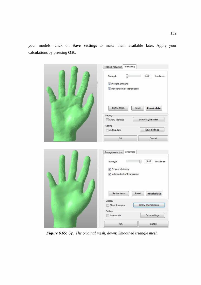
132
your models, click on Save settings to make them available later. Apply your
calculations by pressing OK.
Figure 6.65: Up: The original mesh, down: Smoothed triangle mesh.
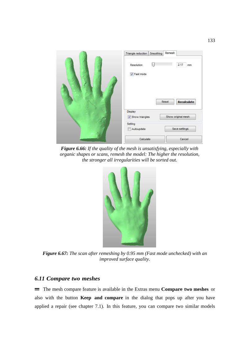
133
Figure 6.67: The scan after remeshing by 0.95 mm (Fast mode unchecked) with an improved surface quality.
6.11 Compare two meshes
The mesh compare feature is available in the Extras menu Compare two meshes or
also with the button Keep and compare in the dialog that pops up after you have
applied a repair (see chapter 7.1). In this feature, you can compare two similar models
Figure 6.66: If the quality of the mesh is unsatisfying, especially with organic shapes or scans, remesh the model: The higher the resolution,
the stronger all irregularities will be sorted out.
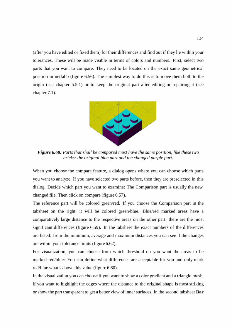
134
(after you have edited or fixed them) for their differences and find out if they lie within your
tolerances. These will be made visible in terms of colors and numbers. First, select two
parts that you want to compare. They need to be located on the exact same geometrical
position in netfabb (figure 6.56). The simplest way to do this is to move them both to the
origin (see chapter 5.5.1) or to keep the original part after editing or repairing it (see
chapter 7.1).
Figure 6.68: Parts that shall be compared must have the same position, like these two bricks: the original blue part and the changed purple part.
When you choose the compare feature, a dialog opens where you can choose which parts
you want to analyze. If you have selected two parts before, then they are preselected in this
dialog. Decide which part you want to examine: The Comparison part is usually the new,
changed file. Then click on compare (figure 6.57).
The reference part will be colored green/red. If you choose the Comparison part in the
tabsheet on the right, it will be colored green/blue. Blue/red marked areas have a
comparatively large distance to the respective areas on the other part: there are the most
significant differences (figure 6.59). In the tabsheet the exact numbers of the differences
are listed: from the minimum, average and maximum distances you can see if the changes
are within your tolerance limits (figure 6.62).
For visualization, you can choose from which threshold on you want the areas to be
marked red/blue: You can define what differences are acceptable for you and only mark
red/blue what’s above this value (figure 6.60).
In the visualization you can choose if you want to show a color gradient and a triangle mesh,
if you want to highlight the edges where the distance to the original shape is most striking
or show the part transparent to get a better view of inner surfaces. In the second tabsheet Bar

135
chart you find listed, how many areas of a part have a specific distance to the original
part. So one bar stands for a distance and the bar’s height displays, how often this distance
occurs.
Figure 6.69: In the compare module: Select in this dialog, which model should be checked for changes. The differences will be made visible on the comparison part.
Figure 6.70: See the minimum, average and maximum distance in this tabsheet and check
if the differences are within your tolerance limits.
Figure 6.71: Left: On the comparison part the most significant differences are marked blue. Right: On the Reference parts, these
areas are marked red.
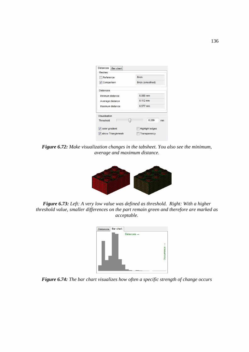
136
Figure 6.72: Make visualization changes in the tabsheet. You also see the minimum, average and maximum distance.
Figure 6.73: Left: A very low value was defined as threshold. Right: With a higher
threshold value, smaller differences on the part remain green and therefore are marked as acceptable.
Figure 6.74: The bar chart visualizes how often a specific strength of change occurs
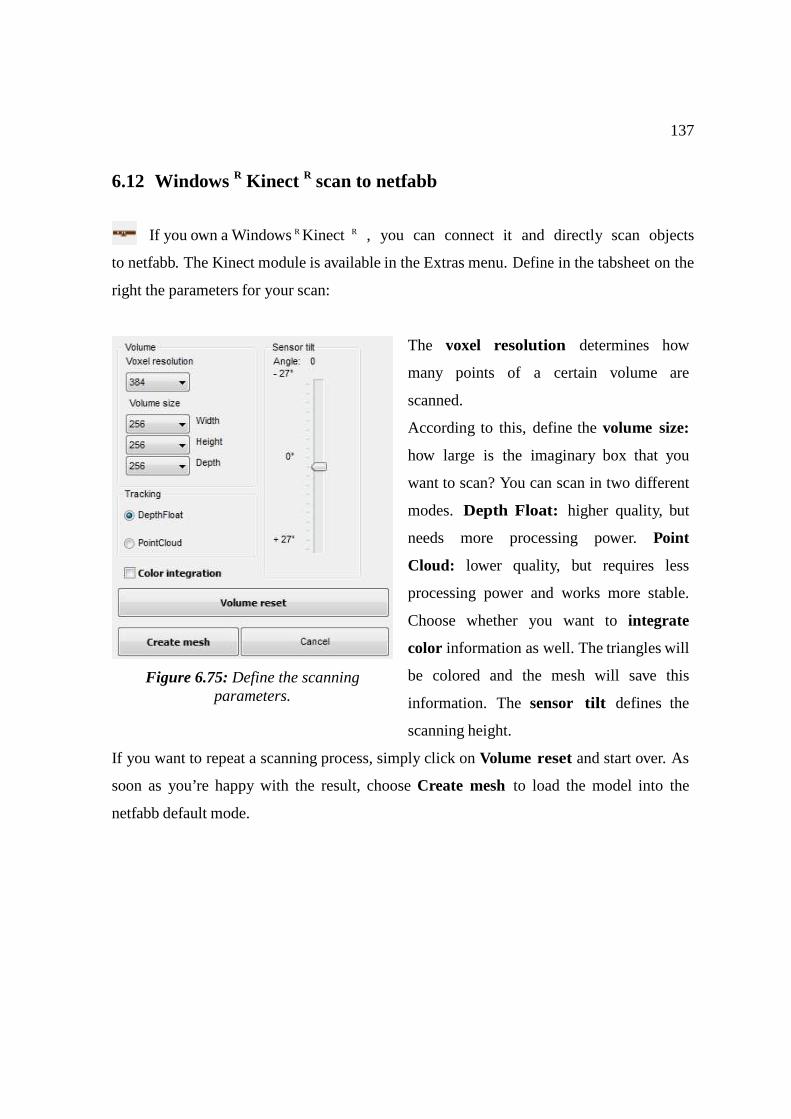
137
6.12 Windows R Kinect R scan to netfabb
If you own a Windows R Kinect R , you can connect it and directly scan objects
to netfabb. The Kinect module is available in the Extras menu. Define in the tabsheet on the
right the parameters for your scan:
Figure 6.75: Define the scanning parameters.
The voxel resolution determines how
many points of a certain volume are
scanned.
According to this, define the volume size:
how large is the imaginary box that you
want to scan? You can scan in two different
modes. Depth Float: higher quality, but
needs more processing power. Point
Cloud: lower quality, but requires less
processing power and works more stable.
Choose whether you want to integrate
color information as well. The triangles will
be colored and the mesh will save this
information. The sensor tilt defines the
scanning height.
If you want to repeat a scanning process, simply click on Volume reset and start over. As
soon as you’re happy with the result, choose Create mesh to load the model into the
netfabb default mode.
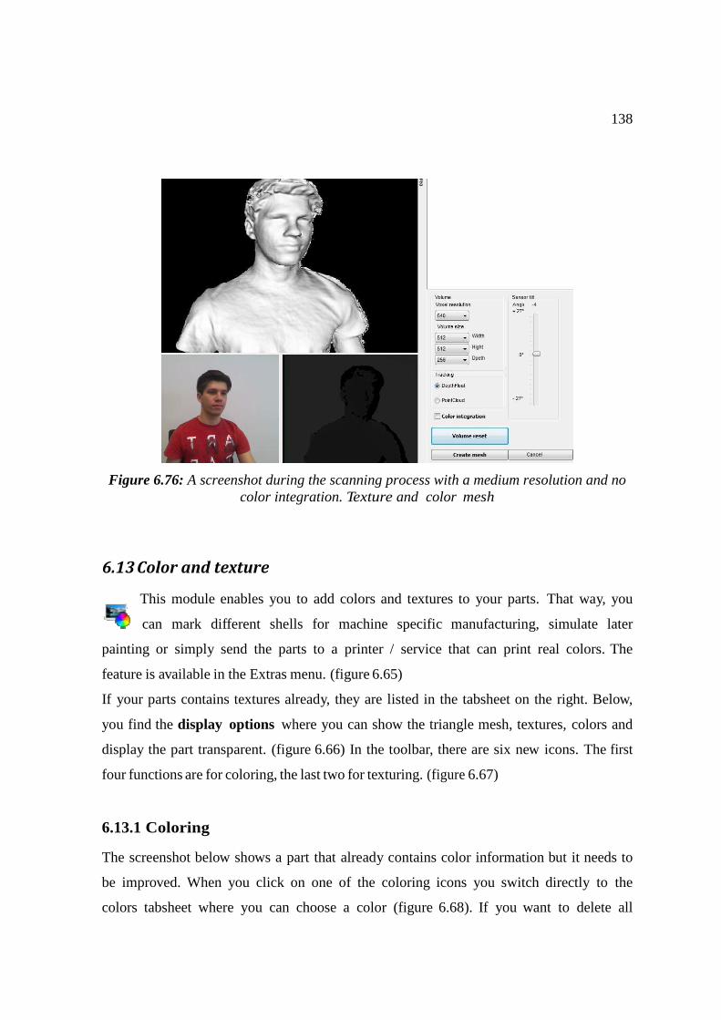
138
Figure 6.76: A screenshot during the scanning process with a medium resolution and no color integration. Texture and color mesh
6.13 Color and texture
This module enables you to add colors and textures to your parts. That way, you
can mark different shells for machine specific manufacturing, simulate later
painting or simply send the parts to a printer / service that can print real colors. The
feature is available in the Extras menu. (figure 6.65)
If your parts contains textures already, they are listed in the tabsheet on the right. Below,
you find the display options where you can show the triangle mesh, textures, colors and
display the part transparent. (figure 6.66) In the toolbar, there are six new icons. The first
four functions are for coloring, the last two for texturing. (figure 6.67)
6.13.1 Coloring
The screenshot below shows a part that already contains color information but it needs to
be improved. When you click on one of the coloring icons you switch directly to the
colors tabsheet where you can choose a color (figure 6.68). If you want to delete all
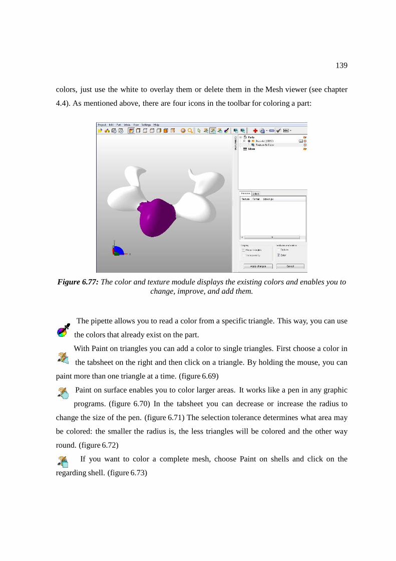
139
colors, just use the white to overlay them or delete them in the Mesh viewer (see chapter
4.4). As mentioned above, there are four icons in the toolbar for coloring a part:
Figure 6.77: The color and texture module displays the existing colors and enables you to change, improve, and add them.
The pipette allows you to read a color from a specific triangle. This way, you can use
the colors that already exist on the part.
With Paint on triangles you can add a color to single triangles. First choose a color in
the tabsheet on the right and then click on a triangle. By holding the mouse, you can
paint more than one triangle at a time. (figure 6.69)
Paint on surface enables you to color larger areas. It works like a pen in any graphic
programs. (figure 6.70) In the tabsheet you can decrease or increase the radius to
change the size of the pen. (figure 6.71) The selection tolerance determines what area may
be colored: the smaller the radius is, the less triangles will be colored and the other way
round. (figure 6.72)
If you want to color a complete mesh, choose Paint on shells and click on the
regarding shell. (figure 6.73)
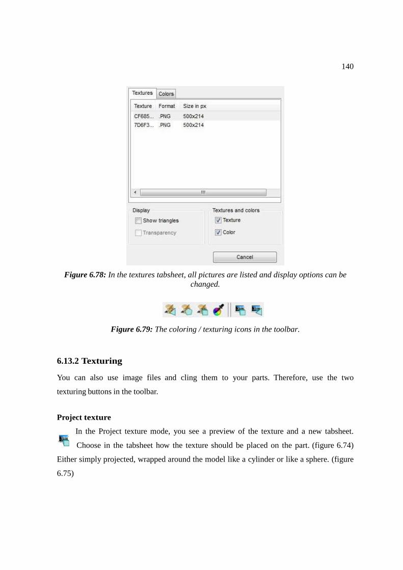
140
Figure 6.78: In the textures tabsheet, all pictures are listed and display options can be changed.
Figure 6.79: The coloring / texturing icons in the toolbar.
6.13.2 Texturing
You can also use image files and cling them to your parts. Therefore, use the two
texturing buttons in the toolbar. Project texture
In the Project texture mode, you see a preview of the texture and a new tabsheet.
Choose in the tabsheet how the texture should be placed on the part. (figure 6.74)
Either simply projected, wrapped around the model like a cylinder or like a sphere. (figure
6.75)
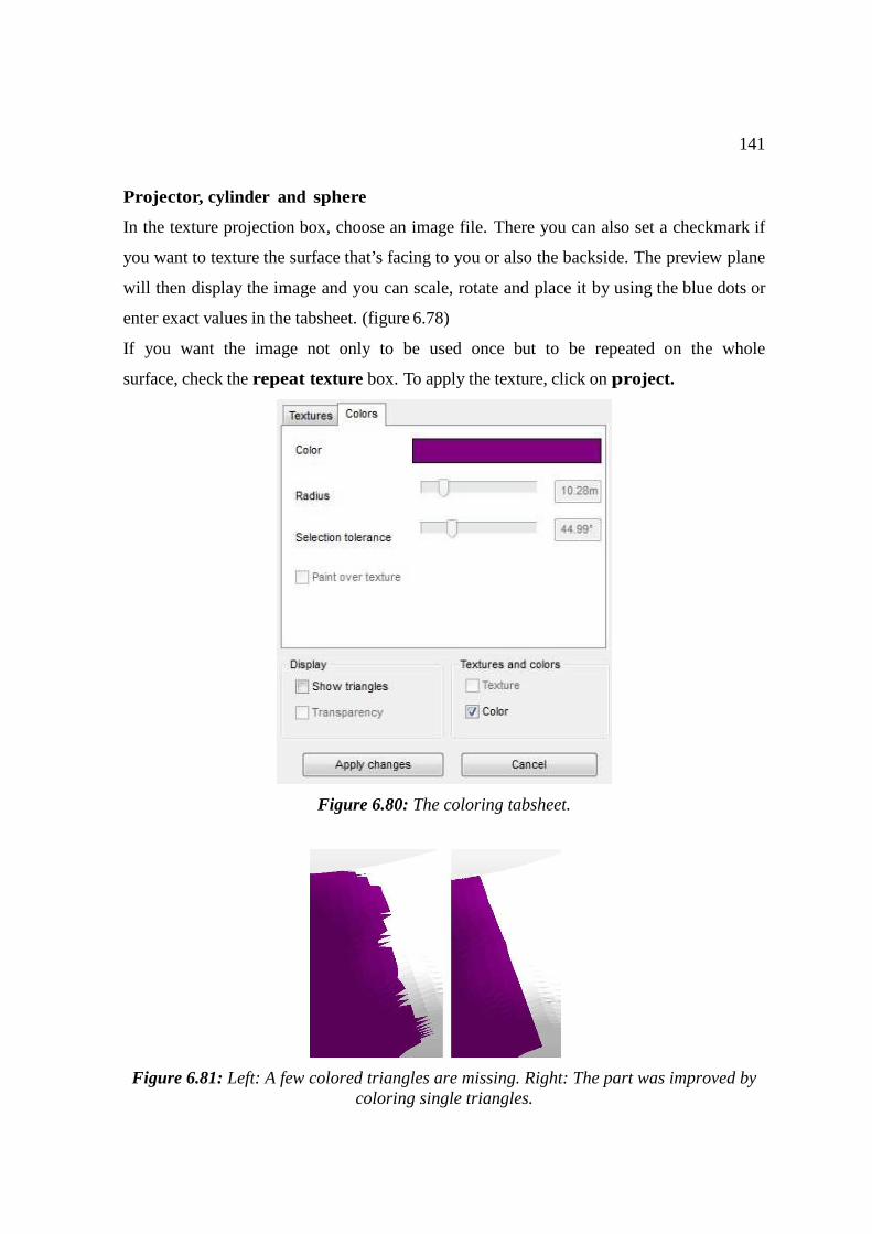
141
Projector, cylinder and sphere
In the texture projection box, choose an image file. There you can also set a checkmark if
you want to texture the surface that’s facing to you or also the backside. The preview plane
will then display the image and you can scale, rotate and place it by using the blue dots or
enter exact values in the tabsheet. (figure 6.78)
If you want the image not only to be used once but to be repeated on the whole
surface, check the repeat texture box. To apply the texture, click on project.
Figure 6.80: The coloring tabsheet.
Figure 6.81: Left: A few colored triangles are missing. Right: The part was improved by coloring single triangles.
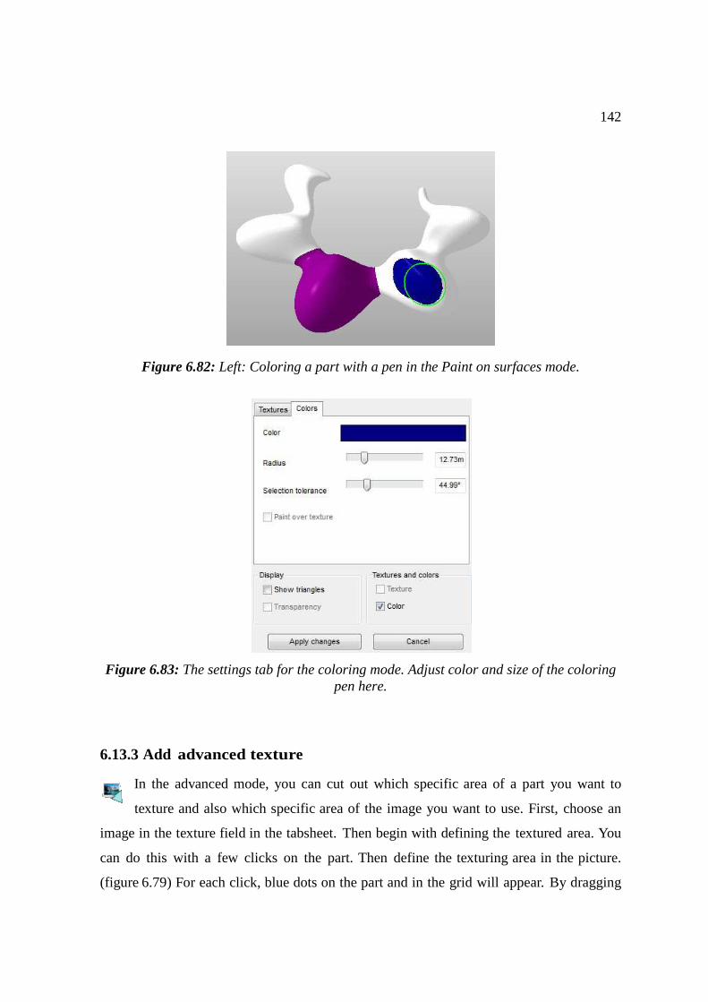
142
Figure 6.82: Left: Coloring a part with a pen in the Paint on surfaces mode.
Figure 6.83: The settings tab for the coloring mode. Adjust color and size of the coloring pen here.
6.13.3 Add advanced texture
In the advanced mode, you can cut out which specific area of a part you want to
texture and also which specific area of the image you want to use. First, choose an
image in the texture field in the tabsheet. Then begin with defining the textured area. You
can do this with a few clicks on the part. Then define the texturing area in the picture.
(figure 6.79) For each click, blue dots on the part and in the grid will appear. By dragging

143
these dots you can define this area more precisely. With a right click on the dots you can
delete or reset the points.
This mode works similar to the projector mode, with one difference: The advanced mode
wraps the image also in undercuts; the projector doesn’t. (figure 6.80)
Figure 6.84: Left: A selection tolerance below 90◦. Right: Here’s the tolerance above 90◦ and the pen now also covers the ancient side of the box.
Figure 6.85: One complete shell colored with the Paint on shell mode.
Figure 6.86: Preview of texture and the texturing tabsheet.

144
Figure 6.87: Left: projector, middle: cylinder, right: sphere.
Figure 6.88: Left: the part with a preview of the texturing plane, middle: a preview of the
texture, right: the textured part.
Figure 6.89: Left: the part with a preview of the texturing plane, middle: a preview of the
texture, right: the textured part.
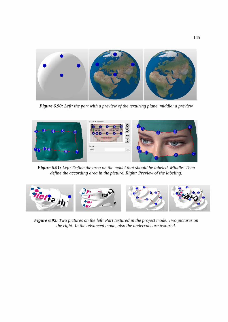
145
Figure 6.90: Left: the part with a preview of the texturing plane, middle: a preview
Figure 6.91: Left: Define the area on the model that should be labeled. Middle: Then define the according area in the picture. Right: Preview of the labeling.
Figure 6.92: Two pictures on the left: Part textured in the project mode. Two pictures on
the right: In the advanced mode, also the undercuts are textured.
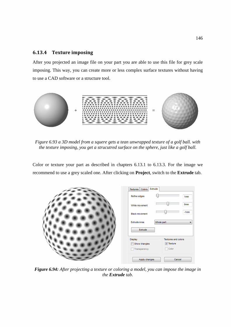
146
6.13.4 Texture imposing
After you projected an image file on your part you are able to use this file for grey scale
imposing. This way, you can create more or less complex surface textures without having
to use a CAD software or a structure tool.
+
=
Figure 6.93 a 3D model from a squere gets a tean unwrapped texture of a golf ball. with the texture imposing, you get a strucutred surface on the sphere, just like a golf ball.
Color or texture your part as described in chapters 6.13.1 to 6.13.3. For the image we
recommend to use a grey scaled one. After clicking on Project, switch to the Extrude tab.
Figure 6.94: After projecting a texture or coloring a model, you can impose the image in the Extrude tab.
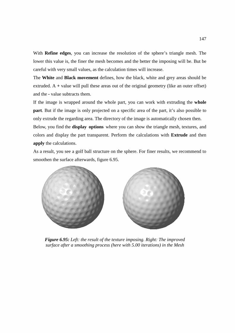
147
With Refine edges, you can increase the resolution of the sphere’s triangle mesh. The
lower this value is, the finer the mesh becomes and the better the imposing will be. But be
careful with very small values, as the calculation times will increase.
The White and Black movement defines, how the black, white and grey areas should be
extruded. A + value will pull these areas out of the original geometry (like an outer offset)
and the - value subtracts them.
If the image is wrapped around the whole part, you can work with extruding the whole
part. But if the image is only projected on a specific area of the part, it’s also possible to
only extrude the regarding area. The directory of the image is automatically chosen then.
Below, you find the display options where you can show the triangle mesh, textures, and
colors and display the part transparent. Perform the calculations with Extrude and then
apply the calculations.
As a result, you see a golf ball structure on the sphere. For finer results, we recommend to
smoothen the surface afterwards, figure 6.95.
Figure 6.95: Left: the result of the texture imposing. Right: The improved surface after a smoothing process (here with 5.00 iterations) in the Mesh
manipulation module.

148
7 Part Repair
7.1 The Repair Module
Whenever any part is damaged and therefore cannot be used for 3D printing, a large
warning sign with an exclamation mark is displayed in the bottom right of the viewing
screen, and a little warning sign is placed next to the part in the project tree (figure 7.1).
Before building these parts, they must be repaired.
The fastest way to repair one or several parts is to select them and click on the
shortcut icon Automatic part repair in the tabsheet on the right. A dialog opens
where you can choose between three predefined repair macros (see chapter 7.6 for more
information on the single scripts.) You can either use these predefined macros or define
your own ones (e.g. with an automatic scaling or naming of parts - see chapter 7.6 also).
Like this, you can automatize and speed up your processes.
For a more controlled repair, select a part and start the repair module with the red
cross icon in toolbar, in the Extras submenu of the context menu or in the Extras
menu in the menu bar.
The viewing screen then switches to the repair screen, which includes only the selected
part. In the tabsheet, you can choose from five registers, "Status", "Actions", "Repair
scripts", "Shells" and "View". In the menu bar, the menus Repair and Mesh Edit are added.
In the project tree, the repair is integrated as subordinate element of the part. After
conducting other operations, you can return to the repair any time by selecting the repair in
the project tree. You can also add other parts to the repair module by drag & drop in the
project tree. That way, you can repair several parts at once.
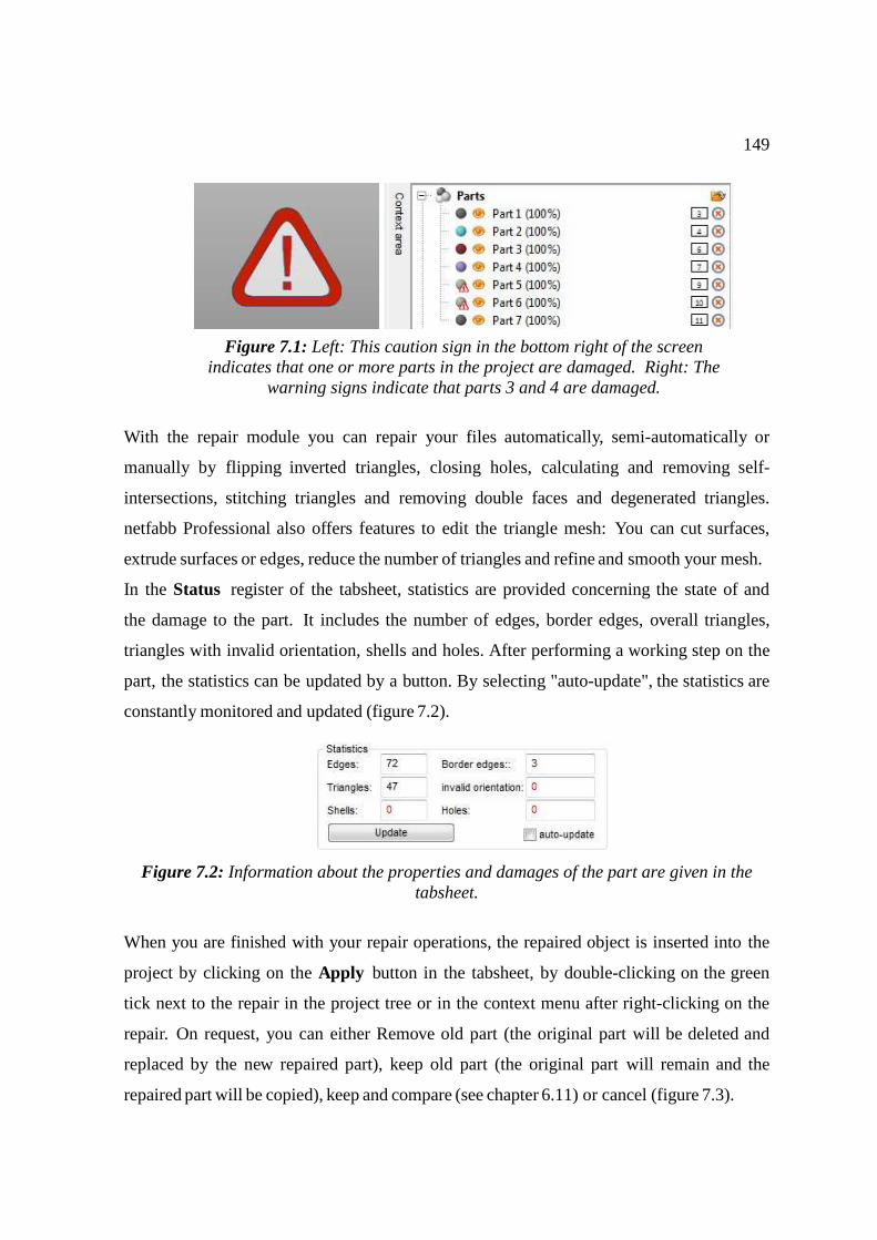
149
With the repair module you can repair your files automatically, semi-automatically or
manually by flipping inverted triangles, closing holes, calculating and removing self-
intersections, stitching triangles and removing double faces and degenerated triangles.
netfabb Professional also offers features to edit the triangle mesh: You can cut surfaces,
extrude surfaces or edges, reduce the number of triangles and refine and smooth your mesh.
In the Status register of the tabsheet, statistics are provided concerning the state of and
the damage to the part. It includes the number of edges, border edges, overall triangles,
triangles with invalid orientation, shells and holes. After performing a working step on the
part, the statistics can be updated by a button. By selecting "auto-update", the statistics are
constantly monitored and updated (figure 7.2).
Figure 7.2: Information about the properties and damages of the part are given in the tabsheet.
When you are finished with your repair operations, the repaired object is inserted into the
project by clicking on the Apply button in the tabsheet, by double-clicking on the green
tick next to the repair in the project tree or in the context menu after right-clicking on the
repair. On request, you can either Remove old part (the original part will be deleted and
replaced by the new repaired part), keep old part (the original part will remain and the
repaired part will be copied), keep and compare (see chapter 6.11) or cancel (figure 7.3).
Figure 7.1: Left: This caution sign in the bottom right of the screen indicates that one or more parts in the project are damaged. Right: The
warning signs indicate that parts 3 and 4 are damaged.
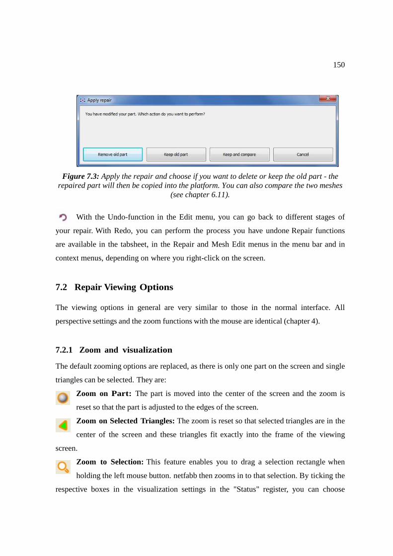
150
Figure 7.3: Apply the repair and choose if you want to delete or keep the old part - the repaired part will then be copied into the platform. You can also compare the two meshes
(see chapter 6.11).
With the Undo-function in the Edit menu, you can go back to different stages of
your repair. With Redo, you can perform the process you have undone Repair functions
are available in the tabsheet, in the Repair and Mesh Edit menus in the menu bar and in
context menus, depending on where you right-click on the screen.
7.2 Repair Viewing Options
The viewing options in general are very similar to those in the normal interface. All
perspective settings and the zoom functions with the mouse are identical (chapter 4).
7.2.1 Zoom and visualization
The default zooming options are replaced, as there is only one part on the screen and single
triangles can be selected. They are:
Zoom on Part: The part is moved into the center of the screen and the zoom is
reset so that the part is adjusted to the edges of the screen.
Zoom on Selected Triangles: The zoom is reset so that selected triangles are in the
center of the screen and these triangles fit exactly into the frame of the viewing
screen.
Zoom to Selection: This feature enables you to drag a selection rectangle when
holding the left mouse button. netfabb then zooms in to that selection. By ticking the
respective boxes in the visualization settings in the "Status" register, you can choose

151
whether to highlight holes with a yellow line, show degenerated faces, visualize the
triangle mesh and highlight errors with a thicker line. Errors can also be highlighted during
operations by holding the H-key (figure 7.4).
Figure 7.4: The visualization settings in the tabsheet
If the triangle mesh is not shown, there is the option to visualize triangle edges exceeding
a certain angle which can be adjusted with a slider. Here, 0◦ stands for triangles lying in
the same plane and all angled edges are shown, while with 180◦ (or off), no edges are
visualized (figure 7.5). The setting of this regulator also has an influence on the selection of
surfaces (see chapter 7.3).
7.2.2 Inner view
In the tab View, you can now take a look inside the part. This is very helpful if you need to
repair a mesh which is hidden in or behind another shell and which you can’t reach from
outside. If your model contains texture information, tick the box Show textures to make
them visible. The next check box turns the whole part transparent and you can see every
shell the model contains. The scroll bars below are the actual viewing tool: move a bar
until you see an outline on the model and click on one half of the little orange box on the
left side of the bar. (figure 7.6) The model will be opened and you can now edit and
repair the interior parts of the file. (For further explanations see chapter 6.4.) A click on
the box Transparent Cuts hides or shows the "cut off" part.
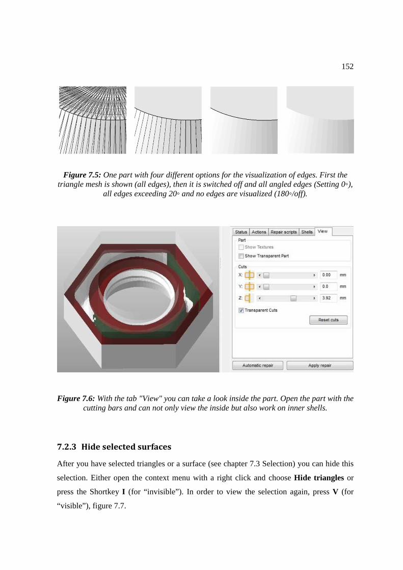
152
Figure 7.5: One part with four different options for the visualization of edges. First the triangle mesh is shown (all edges), then it is switched off and all angled edges (Setting 0◦),
all edges exceeding 20◦ and no edges are visualized (180◦/off).
Figure 7.6: With the tab "View" you can take a look inside the part. Open the part with the cutting bars and can not only view the inside but also work on inner shells.
7.2.3 Hide selected surfaces
After you have selected triangles or a surface (see chapter 7.3 Selection) you can hide this
selection. Either open the context menu with a right click and choose Hide triangles or
press the Shortkey I (for “invisible”). In order to view the selection again, press V (for
“visible”), figure 7.7.
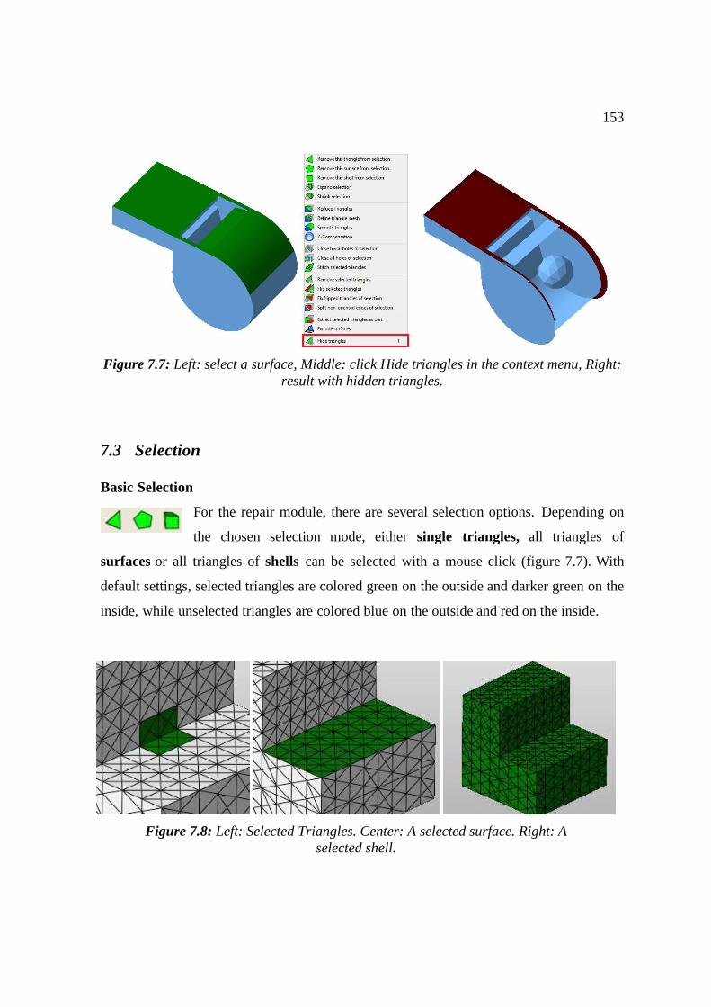
153
Figure 7.7: Left: select a surface, Middle: click Hide triangles in the context menu, Right: result with hidden triangles.
7.3 Selection
Basic Selection
For the repair module, there are several selection options. Depending on
the chosen selection mode, either single triangles, all triangles of
surfaces or all triangles of shells can be selected with a mouse click (figure 7.7). With
default settings, selected triangles are colored green on the outside and darker green on the
inside, while unselected triangles are colored blue on the outside and red on the inside.
Figure 7.8: Left: Selected Triangles. Center: A selected surface. Right: A selected shell.
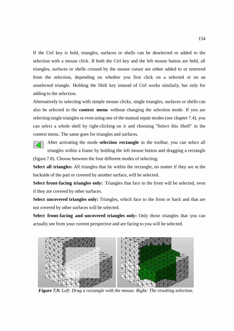
154
If the Ctrl key is held, triangles, surfaces or shells can be deselected or added to the
selection with a mouse click. If both the Ctrl key and the left mouse button are held, all
triangles, surfaces or shells crossed by the mouse cursor are either added to or removed
from the selection, depending on whether you first click on a selected or on an
unselected triangle. Holding the Shift key instead of Ctrl works similarly, but only for
adding to the selection.
Alternatively to selecting with simple mouse clicks, single triangles, surfaces or shells can
also be selected in the context menu without changing the selection mode. If you are
selecting single triangles or even using one of the manual repair modes (see chapter 7.4), you
can select a whole shell by right-clicking on it and choosing "Select this Shell" in the
context menu. The same goes for triangles and surfaces.
After activating the mode selection rectangle in the toolbar, you can select all
triangles within a frame by holding the left mouse button and dragging a rectangle
(figure 7.8). Choose between the four different modes of selecting:
Select all triangles: All triangles that lie within the rectangle, no matter if they are at the
backside of the part or covered by another surface, will be selected.
Select front-facing triangles only: Triangles that face to the front will be selected, even
if they are covered by other surfaces.
Select uncovered triangles only: Triangles, which face to the front or back and that are
not covered by other surfaces will be selected.
Select front-facing and uncovered triangles only: Only those triangles that you can
actually see from your current perspective and are facing to you will be selected.
Figure 7.9: Left: Drag a rectangle with the mouse. Right: The resulting selection.
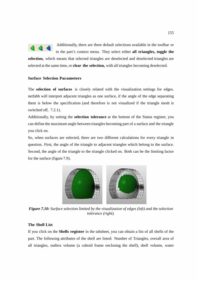
155
Additionally, there are three default selections available in the toolbar or
in the part’s context menu. They select either all triangles, toggle the
selection, which means that selected triangles are deselected and deselected triangles are
selected at the same time, or clear the selection, with all triangles becoming deselected. Surface Selection Parameters
The selection of surfaces is closely related with the visualization settings for edges.
netfabb will interpret adjacent triangles as one surface, if the angle of the edge separating
them is below the specification (and therefore is not visualized if the triangle mesh is
switched off, 7.2.1).
Additionally, by setting the selection tolerance at the bottom of the Status register, you
can define the maximum angle between triangles becoming part of a surface and the triangle
you click on.
So, when surfaces are selected, there are two different calculations for every triangle in
question. First, the angle of the triangle to adjacent triangles which belong to the surface.
Second, the angle of the triangle to the triangle clicked on. Both can be the limiting factor
for the surface (figure 7.9).
Figure 7.10: Surface selection limited by the visualization of edges (left) and the selection tolerance (right).
The Shell List
If you click on the Shells register in the tabsheet, you can obtain a list of all shells of the
part. The following attributes of the shell are listed: Number of Triangles, overall area of
all triangles, outbox volume (a cuboid frame enclosing the shell), shell volume, water
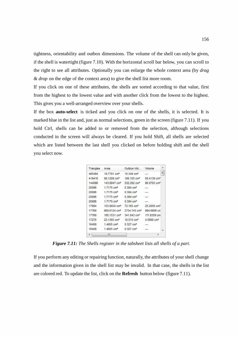
156
tightness, orientability and outbox dimensions. The volume of the shell can only be given,
if the shell is watertight (figure 7.10). With the horizontal scroll bar below, you can scroll to
the right to see all attributes. Optionally you can enlarge the whole context area (by drag
& drop on the edge of the context area) to give the shell list more room.
If you click on one of these attributes, the shells are sorted according to that value, first
from the highest to the lowest value and with another click from the lowest to the highest.
This gives you a well-arranged overview over your shells.
If the box auto-select is ticked and you click on one of the shells, it is selected. It is
marked blue in the list and, just as normal selections, green in the screen (figure 7.11). If you
hold Ctrl, shells can be added to or removed from the selection, although selections
conducted in the screen will always be cleared. If you hold Shift, all shells are selected
which are listed between the last shell you clicked on before holding shift and the shell
you select now.
Figure 7.11: The Shells register in the tabsheet lists all shells of a part.
If you perform any editing or repairing function, naturally, the attributes of your shell change
and the information given in the shell list may be invalid. In that case, the shells in the list
are colored red. To update the list, click on the Refresh button below (figure 7.11).
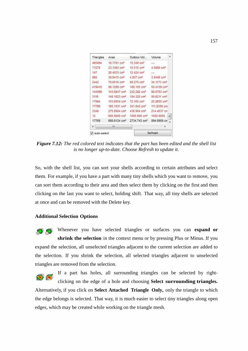
157
Figure 7.12: The red colored text indicates that the part has been edited and the shell list is no longer up-to-date. Choose Refresh to update it.
So, with the shell list, you can sort your shells according to certain attributes and select
them. For example, if you have a part with many tiny shells which you want to remove, you
can sort them according to their area and then select them by clicking on the first and then
clicking on the last you want to select, holding shift. That way, all tiny shells are selected
at once and can be removed with the Delete key.
Additional Selection Options
Whenever you have selected triangles or surfaces you can expand or
shrink the selection in the context menu or by pressing Plus or Minus. If you
expand the selection, all unselected triangles adjacent to the current selection are added to
the selection. If you shrink the selection, all selected triangles adjacent to unselected
triangles are removed from the selection.
If a part has holes, all surrounding triangles can be selected by right-
clicking on the edge of a hole and choosing Select surrounding triangles.
Alternatively, if you click on Select Attached Triangle Only, only the triangle to which
the edge belongs is selected. That way, it is much easier to select tiny triangles along open
edges, which may be created while working on the triangle mesh.

158
In the Actions register, the button Select Shells with Negative Volume enables the user
to select all inverted shells. This function is very useful to select and then invert or remove
those shells. However, it is only reliable for closed and oriented shells.
Finally, you can perform an advanced triangle selection. Choose the option in the
context menu and use the dialog box to select or deselect triangles above or below (or
both) a certain area, volume (of the shell) and edge length (figure 7.12).
Figure 7.13: The dialog box for the advanced triangle selection
7.4 Manual Repair
With manual repair operations you can perform simple repair and mesh editing jobs. The
manual operations are available in the toolbar. "Remove selected triangles" and "Flip
selected triangles" are also available in the Repair menu and in the context menu, if you
right-click on a selected triangle.
Add triangles: This mode enables you to close holes manually or to connect edges.
A triangle is created by first clicking on a border edge of a triangle, which is then
marked in a blue color. Now, if you move the mouse across another border edge, you get
a green preview of potentially added triangles. By clicking on another border edge,
triangles are inserted. If the two edges you clicked on are connected by a common corner
point, it is one triangle. If they are not connected, two triangles are inserted. If any border
edges of the new triangles are neighboring other border edges, these are connected
automatically (figure 7.13).

159
Figure 7.14: Add triangles: First, a blue marking of the first selected edge. Second, a projection of the new triangles. Third, the resulting triangles.
Add nodes: In effect, this mode enables the user to refine the triangle mesh
manually by inserting new corner points. A corner point can be inserted by a
mouse click on a triangle. New edges are inserted, connecting this point with the three
corner points of the old triangle. So, one triangle is split into three (figure 7.14). If a node is
placed on an edge, both adjacent triangles are split into two triangles. As long as the left
mouse button is held down, the node is not placed and can be moved across the surface to
the favored position. At the same time, you can see a bright blue preview of the new
triangles. The shape of the part does not change, though the nodes can play a vital role
during further repair operations.
Figure 7.15: A node is added in the middle of a triangle.
Move nodes: netfabb is basically a software for file preparation, not for
constructing. Holes and other errors therefore are repaired in the simplest way: A hole is
usually closed by a plane, a curve won’t be adapted. This can cause troubles, especially

160
with scans. (figure 7.15) But with the Move nodes mode you can easily tweak the model
and tinker the curves.
Figure 7.16: Left: A scan with holes. Middle: Holes are usually closed by a plane. Right: detailed view on the plane. - You can tweak these surfaces and reproduce the curves (see
below).
When the mesh is very irregular, you should add nodes on the plane first (see Add nodes
above). Then choose the move nodes mode and pull the nodes with the mouse. (figure 7.16)
Then you can continue repairing the file. You can for example delete unwanted bumps,
close the holes (figure 7.17) and smooth the new surface (figure 7.18).
Figure 7.17: Left: Add nodes first to have better control over the mesh. Right: Pull the nodes with the mouse.
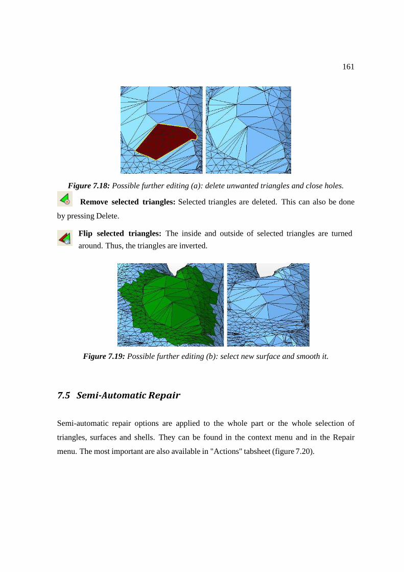
161
Figure 7.18: Possible further editing (a): delete unwanted triangles and close holes.
Remove selected triangles: Selected triangles are deleted. This can also be done
by pressing Delete.
Flip selected triangles: The inside and outside of selected triangles are turned
around. Thus, the triangles are inverted.
Figure 7.19: Possible further editing (b): select new surface and smooth it.
7.5 Semi-Automatic Repair
Semi-automatic repair options are applied to the whole part or the whole selection of
triangles, surfaces and shells. They can be found in the context menu and in the Repair
menu. The most important are also available in "Actions" tabsheet (figure 7.20).

162
7.5.1 Close Holes
There are three ways to close holes without manually inserting the missing triangles.
First, after right-clicking on the edge of a hole (marked yellow, if the visualization
option "Highlight Holes" is activated), you can choose the option Close Hole in the
context menu. Thus, single holes can be closed (figure 7.20). The triangles inserted to fill
the hole are automatically selected.
By clicking on Close trivial holes, all holes are closed that require either one single
triangle or for which only two border edges with the same corner point coordinates have to
be connected.
By clicking Close all holes, all holes of the part are closed automatically. This is
surely the simplest method to repair holes. However, with complicated holes regarding
geometry or orientation, it may lead to unsatisfactory results (figure 7.21).
Figure 7.20: Repair context menu and Actions tabsheet
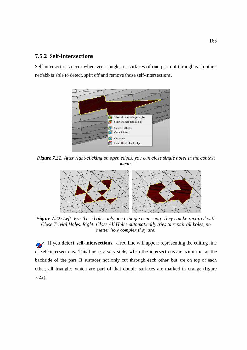
163
7.5.2 Self-Intersections
Self-intersections occur whenever triangles or surfaces of one part cut through each other.
netfabb is able to detect, split off and remove those self-intersections.
Figure 7.21: After right-clicking on open edges, you can close single holes in the context menu.
Figure 7.22: Left: For these holes only one triangle is missing. They can be repaired with Close Trivial Holes. Right: Close All Holes automatically tries to repair all holes, no
matter how complex they are.
If you detect self-intersections, a red line will appear representing the cutting line
of self-intersections. This line is also visible, when the intersections are within or at the
backside of the part. If surfaces not only cut through each other, but are on top of each
other, all triangles which are part of that double surfaces are marked in orange (figure
7.22).
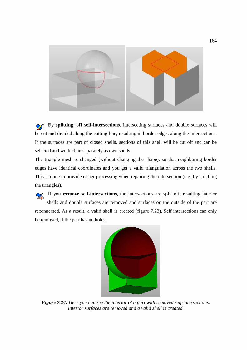
164
By splitting off self-intersections, intersecting surfaces and double surfaces will
be cut and divided along the cutting line, resulting in border edges along the intersections.
If the surfaces are part of closed shells, sections of this shell will be cut off and can be
selected and worked on separately as own shells.
The triangle mesh is changed (without changing the shape), so that neighboring border
edges have identical coordinates and you get a valid triangulation across the two shells.
This is done to provide easier processing when repairing the intersection (e.g. by stitching
the triangles).
If you remove self-intersections, the intersections are split off, resulting interior
shells and double surfaces are removed and surfaces on the outside of the part are
reconnected. As a result, a valid shell is created (figure 7.23). Self intersections can only
be removed, if the part has no holes.
Figure 7.24: Here you can see the interior of a part with removed self-intersections. Interior surfaces are removed and a valid shell is created.
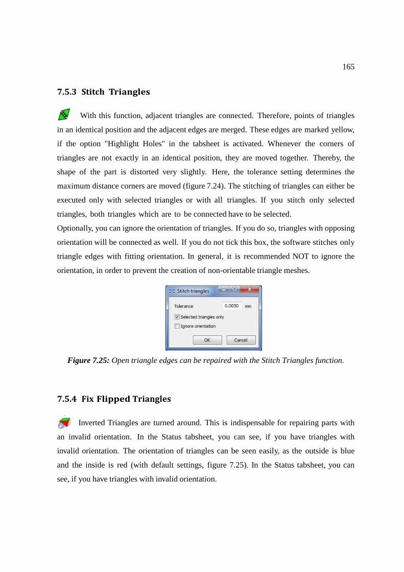
165
7.5.3 Stitch Triangles
With this function, adjacent triangles are connected. Therefore, points of triangles
in an identical position and the adjacent edges are merged. These edges are marked yellow,
if the option "Highlight Holes" in the tabsheet is activated. Whenever the corners of
triangles are not exactly in an identical position, they are moved together. Thereby, the
shape of the part is distorted very slightly. Here, the tolerance setting determines the
maximum distance corners are moved (figure 7.24). The stitching of triangles can either be
executed only with selected triangles or with all triangles. If you stitch only selected
triangles, both triangles which are to be connected have to be selected.
Optionally, you can ignore the orientation of triangles. If you do so, triangles with opposing
orientation will be connected as well. If you do not tick this box, the software stitches only
triangle edges with fitting orientation. In general, it is recommended NOT to ignore the
orientation, in order to prevent the creation of non-orientable triangle meshes.
Figure 7.25: Open triangle edges can be repaired with the Stitch Triangles function.
7.5.4 Fix Flipped Triangles
Inverted Triangles are turned around. This is indispensable for repairing parts with
an invalid orientation. In the Status tabsheet, you can see, if you have triangles with
invalid orientation. The orientation of triangles can be seen easily, as the outside is blue
and the inside is red (with default settings, figure 7.25). In the Status tabsheet, you can
see, if you have triangles with invalid orientation.
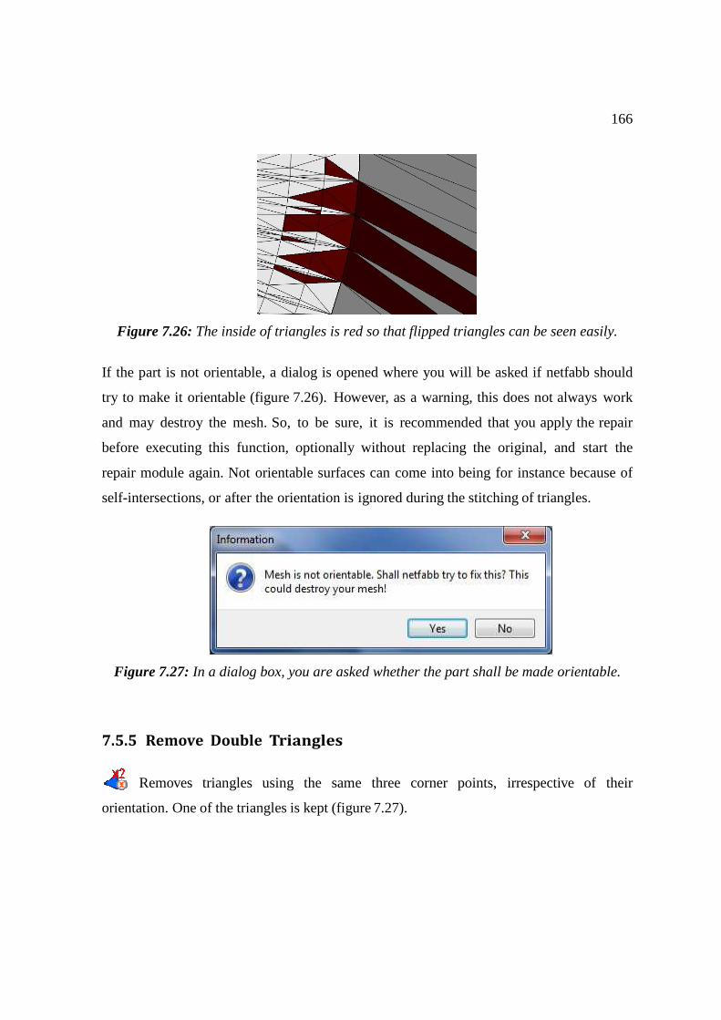
166
Figure 7.26: The inside of triangles is red so that flipped triangles can be seen easily.
If the part is not orientable, a dialog is opened where you will be asked if netfabb should
try to make it orientable (figure 7.26). However, as a warning, this does not always work
and may destroy the mesh. So, to be sure, it is recommended that you apply the repair
before executing this function, optionally without replacing the original, and start the
repair module again. Not orientable surfaces can come into being for instance because of
self-intersections, or after the orientation is ignored during the stitching of triangles.
Figure 7.27: In a dialog box, you are asked whether the part shall be made orientable.
7.5.5 Remove Double Triangles
Removes triangles using the same three corner points, irrespective of their
orientation. One of the triangles is kept (figure 7.27).
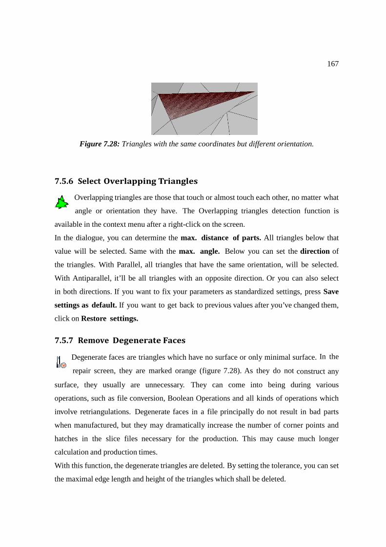
167
Figure 7.28: Triangles with the same coordinates but different orientation.
7.5.6 Select Overlapping Triangles
Overlapping triangles are those that touch or almost touch each other, no matter what
angle or orientation they have. The Overlapping triangles detection function is
available in the context menu after a right-click on the screen.
In the dialogue, you can determine the max. distance of parts. All triangles below that
value will be selected. Same with the max. angle. Below you can set the direction of
the triangles. With Parallel, all triangles that have the same orientation, will be selected.
With Antiparallel, it’ll be all triangles with an opposite direction. Or you can also select
in both directions. If you want to fix your parameters as standardized settings, press Save
settings as default. If you want to get back to previous values after you’ve changed them,
click on Restore settings.
7.5.7 Remove Degenerate Faces
Degenerate faces are triangles which have no surface or only minimal surface. In the
repair screen, they are marked orange (figure 7.28). As they do not construct any
surface, they usually are unnecessary. They can come into being during various
operations, such as file conversion, Boolean Operations and all kinds of operations which
involve retriangulations. Degenerate faces in a file principally do not result in bad parts
when manufactured, but they may dramatically increase the number of corner points and
hatches in the slice files necessary for the production. This may cause much longer
calculation and production times.
With this function, the degenerate triangles are deleted. By setting the tolerance, you can set
the maximal edge length and height of the triangles which shall be deleted.
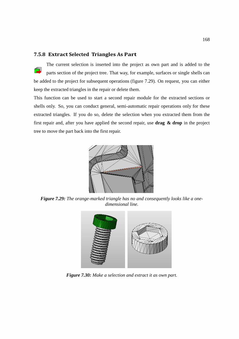
168
7.5.8 Extract Selected Triangles As Part
The current selection is inserted into the project as own part and is added to the
parts section of the project tree. That way, for example, surfaces or single shells can
be added to the project for subsequent operations (figure 7.29). On request, you can either
keep the extracted triangles in the repair or delete them.
This function can be used to start a second repair module for the extracted sections or
shells only. So, you can conduct general, semi-automatic repair operations only for these
extracted triangles. If you do so, delete the selection when you extracted them from the
first repair and, after you have applied the second repair, use drag & drop in the project
tree to move the part back into the first repair.
Figure 7.29: The orange-marked triangle has no and consequently looks like a one-dimensional line.
Figure 7.30: Make a selection and extract it as own part.
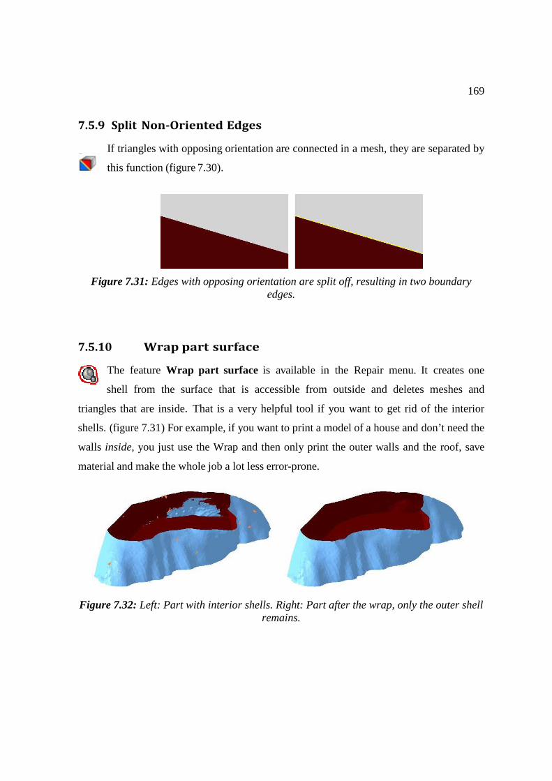
169
7.5.9 Split Non-Oriented Edges
If triangles with opposing orientation are connected in a mesh, they are separated by
this function (figure 7.30).
Figure 7.31: Edges with opposing orientation are split off, resulting in two boundary edges.
7.5.10 Wrap part surface
The feature Wrap part surface is available in the Repair menu. It creates one
shell from the surface that is accessible from outside and deletes meshes and
triangles that are inside. That is a very helpful tool if you want to get rid of the interior
shells. (figure 7.31) For example, if you want to print a model of a house and don’t need the
walls inside, you just use the Wrap and then only print the outer walls and the roof, save
material and make the whole job a lot less error-prone.
Figure 7.32: Left: Part with interior shells. Right: Part after the wrap, only the outer shell remains.
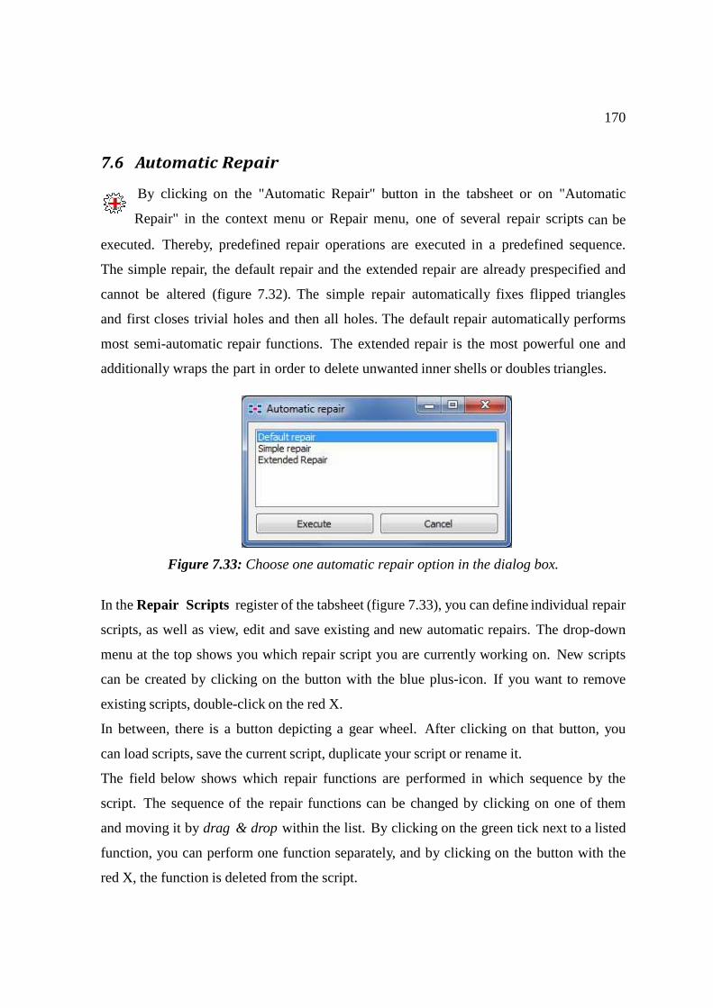
170
7.6 Automatic Repair
By clicking on the "Automatic Repair" button in the tabsheet or on "Automatic
Repair" in the context menu or Repair menu, one of several repair scripts can be
executed. Thereby, predefined repair operations are executed in a predefined sequence.
The simple repair, the default repair and the extended repair are already prespecified and
cannot be altered (figure 7.32). The simple repair automatically fixes flipped triangles
and first closes trivial holes and then all holes. The default repair automatically performs
most semi-automatic repair functions. The extended repair is the most powerful one and
additionally wraps the part in order to delete unwanted inner shells or doubles triangles.
Figure 7.33: Choose one automatic repair option in the dialog box.
In the Repair Scripts register of the tabsheet (figure 7.33), you can define individual repair
scripts, as well as view, edit and save existing and new automatic repairs. The drop-down
menu at the top shows you which repair script you are currently working on. New scripts
can be created by clicking on the button with the blue plus-icon. If you want to remove
existing scripts, double-click on the red X.
In between, there is a button depicting a gear wheel. After clicking on that button, you
can load scripts, save the current script, duplicate your script or rename it.
The field below shows which repair functions are performed in which sequence by the
script. The sequence of the repair functions can be changed by clicking on one of them
and moving it by drag & drop within the list. By clicking on the green tick next to a listed
function, you can perform one function separately, and by clicking on the button with the
red X, the function is deleted from the script.
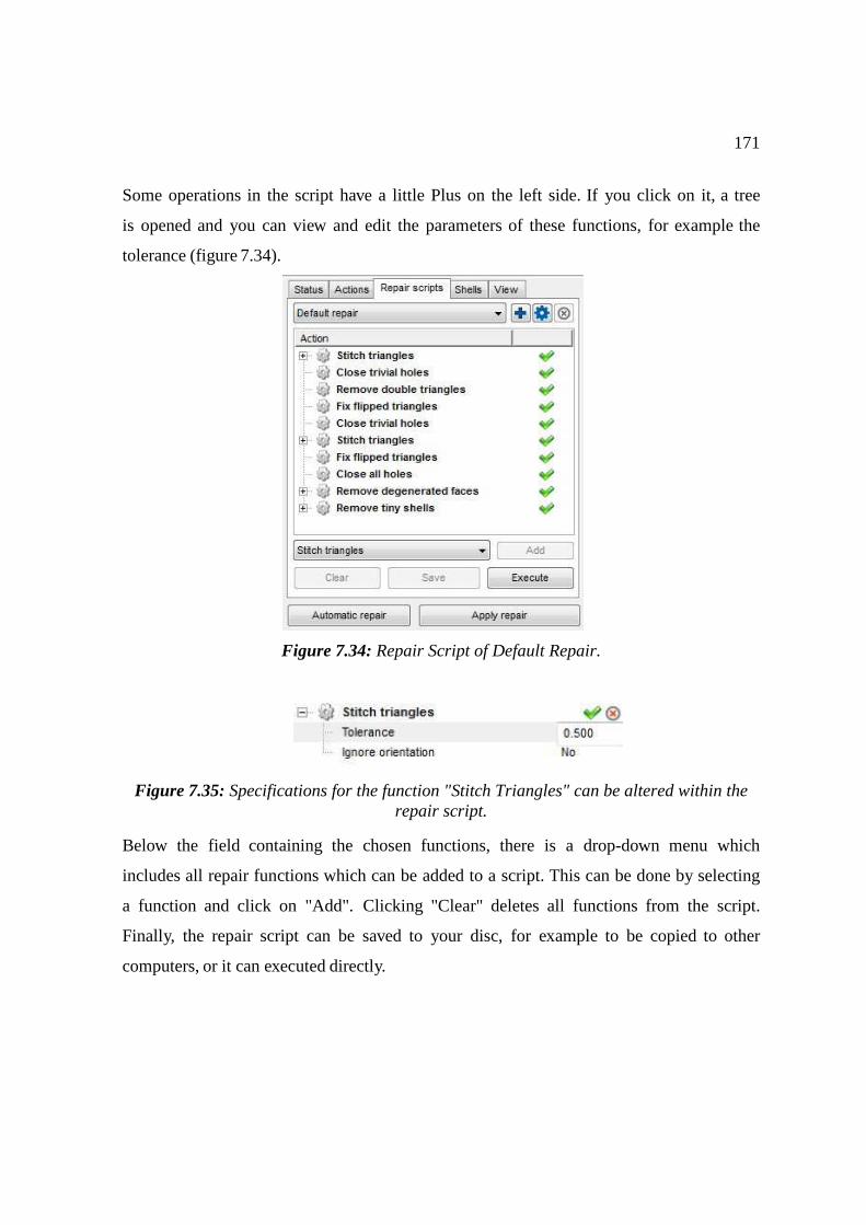
171
Some operations in the script have a little Plus on the left side. If you click on it, a tree
is opened and you can view and edit the parameters of these functions, for example the
tolerance (figure 7.34).
Figure 7.34: Repair Script of Default Repair.
Figure 7.35: Specifications for the function "Stitch Triangles" can be altered within the
repair script.
Below the field containing the chosen functions, there is a drop-down menu which
includes all repair functions which can be added to a script. This can be done by selecting
a function and click on "Add". Clicking "Clear" deletes all functions from the script.
Finally, the repair script can be saved to your disc, for example to be copied to other
computers, or it can executed directly.
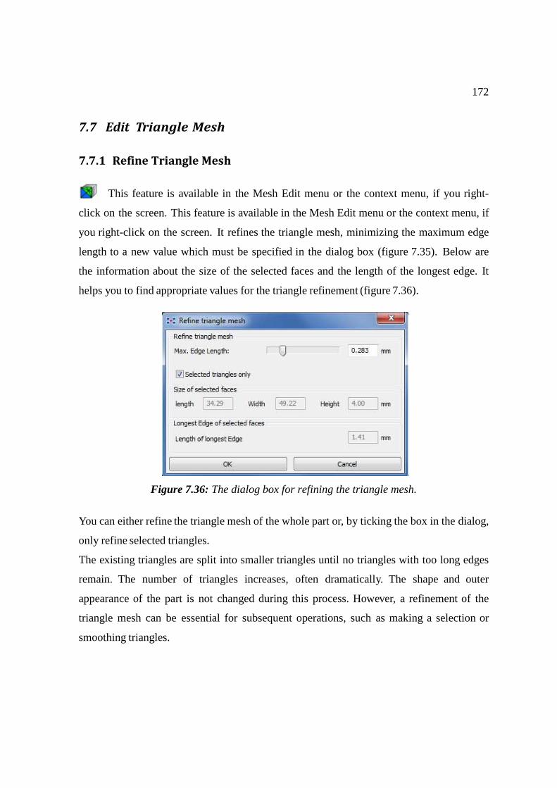
172
7.7 Edit Triangle Mesh
7.7.1 Refine Triangle Mesh
This feature is available in the Mesh Edit menu or the context menu, if you right-
click on the screen. This feature is available in the Mesh Edit menu or the context menu, if
you right-click on the screen. It refines the triangle mesh, minimizing the maximum edge
length to a new value which must be specified in the dialog box (figure 7.35). Below are
the information about the size of the selected faces and the length of the longest edge. It
helps you to find appropriate values for the triangle refinement (figure 7.36).
Figure 7.36: The dialog box for refining the triangle mesh.
You can either refine the triangle mesh of the whole part or, by ticking the box in the dialog,
only refine selected triangles.
The existing triangles are split into smaller triangles until no triangles with too long edges
remain. The number of triangles increases, often dramatically. The shape and outer
appearance of the part is not changed during this process. However, a refinement of the
triangle mesh can be essential for subsequent operations, such as making a selection or
smoothing triangles.

173
Figure 7.37: The triangle mesh of the selected side walls of this cube is refined.
7.7.2 Reduce Triangles
This feature can be found in the Mesh Edit menu or in the context menu after right-
clicking on a selected triangle. You have to have at least 5 triangles selected for
this function. In the triangle reduction, netfabb unifies triangles to create bigger one. When
you start the function, a dialog box appears with the tabs "Basic Reduction" and
"Advanced Reduction". The basic mode is useful, as it proceeds very quickly. If you need
more accurate results, we recommend to use the advanced mode.
In both dialog boxes, you can see how many triangles are selected and you can set, if you
want to reduce the triangle count to a certain target count or if you simply want to reach
the lowest possible number of triangles. If the triangle mesh is very much finer than
necessary, it is recommended to conduct the triangle reduction in several steps, for
example halving the triangle count. Otherwise, you may get unwanted side effect like
double surfaces (figure 7.37).
Below, there are a few important condition you can define for the triangle reduction. The
maximum deformation represents the maximum change in volume of the part. The
maximum collapsed edge length determines the maximum length of edges which are
unified. Please note that wrong condition settings, for example extremely high values,
may lead to unsatisfying results, such as strong distortion or self-intersections (figure 7.38).
In the advanced reduction you can choose the Fast mode", which works faster but a little less
accurate. This is very useful if you just want to test reduction figures.
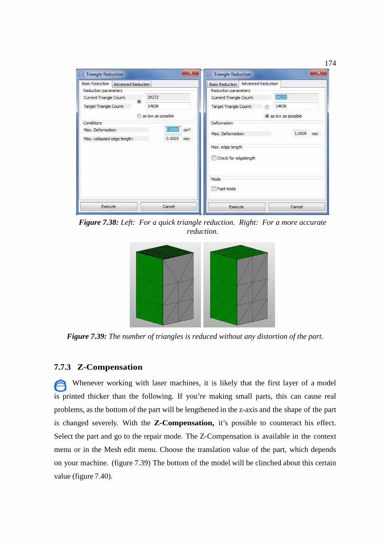
174
Figure 7.39: The number of triangles is reduced without any distortion of the part.
7.7.3 Z-Compensation
Whenever working with laser machines, it is likely that the first layer of a model
is printed thicker than the following. If you’re making small parts, this can cause real
problems, as the bottom of the part will be lengthened in the z-axis and the shape of the part
is changed severely. With the Z-Compensation, it’s possible to counteract his effect.
Select the part and go to the repair mode. The Z-Compensation is available in the context
menu or in the Mesh edit menu. Choose the translation value of the part, which depends
on your machine. (figure 7.39) The bottom of the model will be clinched about this certain
value (figure 7.40).
Figure 7.38: Left: For a quick triangle reduction. Right: For a more accurate reduction.
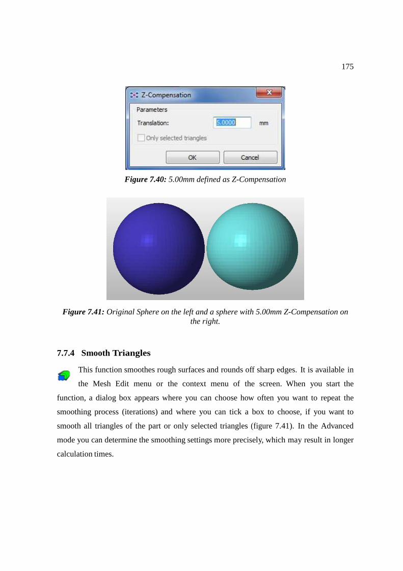
175
Figure 7.40: 5.00mm defined as Z-Compensation
Figure 7.41: Original Sphere on the left and a sphere with 5.00mm Z-Compensation on
the right.
7.7.4 Smooth Triangles
This function smoothes rough surfaces and rounds off sharp edges. It is available in
the Mesh Edit menu or the context menu of the screen. When you start the
function, a dialog box appears where you can choose how often you want to repeat the
smoothing process (iterations) and where you can tick a box to choose, if you want to
smooth all triangles of the part or only selected triangles (figure 7.41). In the Advanced
mode you can determine the smoothing settings more precisely, which may result in longer
calculation times.
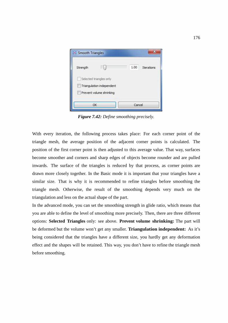
176
Figure 7.42: Define smoothing precisely.
With every iteration, the following process takes place: For each corner point of the
triangle mesh, the average position of the adjacent corner points is calculated. The
position of the first corner point is then adjusted to this average value. That way, surfaces
become smoother and corners and sharp edges of objects become rounder and are pulled
inwards. The surface of the triangles is reduced by that process, as corner points are
drawn more closely together. In the Basic mode it is important that your triangles have a
similar size. That is why it is recommended to refine triangles before smoothing the
triangle mesh. Otherwise, the result of the smoothing depends very much on the
triangulation and less on the actual shape of the part.
In the advanced mode, you can set the smoothing strength in glide ratio, which means that
you are able to define the level of smoothing more precisely. Then, there are three different
options: Selected Triangles only: see above. Prevent volume shrinking: The part will
be deformed but the volume won’t get any smaller. Triangulation independent: As it’s
being considered that the triangles have a different size, you hardly get any deformation
effect and the shapes will be retained. This way, you don’t have to refine the triangle mesh
before smoothing.
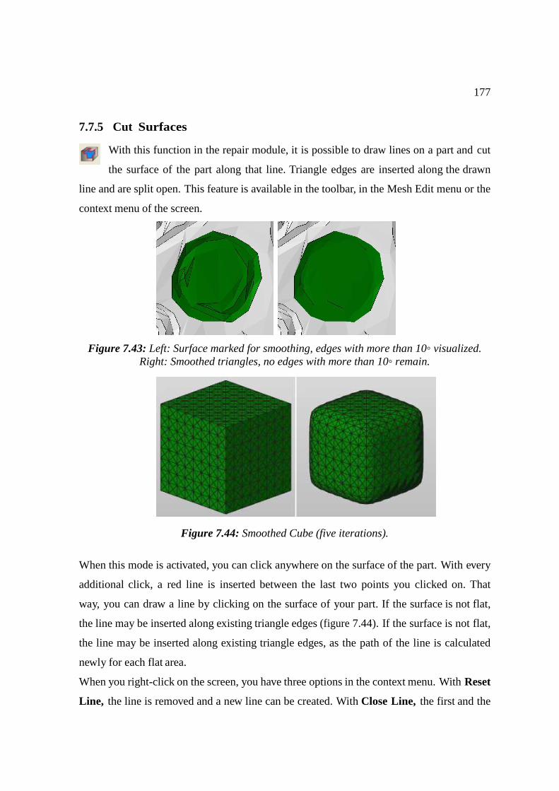
177
7.7.5 Cut Surfaces
With this function in the repair module, it is possible to draw lines on a part and cut
the surface of the part along that line. Triangle edges are inserted along the drawn
line and are split open. This feature is available in the toolbar, in the Mesh Edit menu or the
context menu of the screen.
Figure 7.43: Left: Surface marked for smoothing, edges with more than 10◦ visualized. Right: Smoothed triangles, no edges with more than 10◦ remain.
Figure 7.44: Smoothed Cube (five iterations).
When this mode is activated, you can click anywhere on the surface of the part. With every
additional click, a red line is inserted between the last two points you clicked on. That
way, you can draw a line by clicking on the surface of your part. If the surface is not flat,
the line may be inserted along existing triangle edges (figure 7.44). If the surface is not flat,
the line may be inserted along existing triangle edges, as the path of the line is calculated
newly for each flat area.
When you right-click on the screen, you have three options in the context menu. With Reset
Line, the line is removed and a new line can be created. With Close Line, the first and the
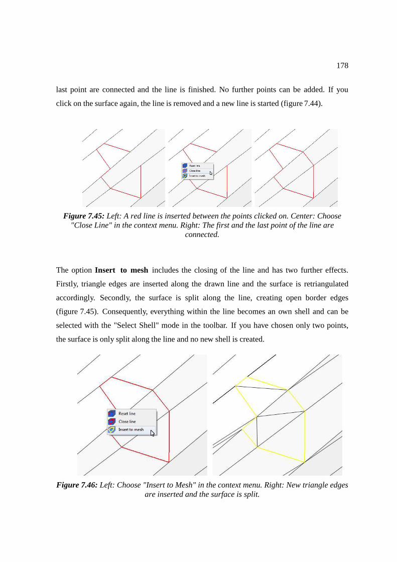
178
last point are connected and the line is finished. No further points can be added. If you
click on the surface again, the line is removed and a new line is started (figure 7.44).
Figure 7.45: Left: A red line is inserted between the points clicked on. Center: Choose "Close Line" in the context menu. Right: The first and the last point of the line are
connected.
The option Insert to mesh includes the closing of the line and has two further effects.
Firstly, triangle edges are inserted along the drawn line and the surface is retriangulated
accordingly. Secondly, the surface is split along the line, creating open border edges
(figure 7.45). Consequently, everything within the line becomes an own shell and can be
selected with the "Select Shell" mode in the toolbar. If you have chosen only two points,
the surface is only split along the line and no new shell is created.
Figure 7.46: Left: Choose "Insert to Mesh" in the context menu. Right: New triangle edges are inserted and the surface is split.
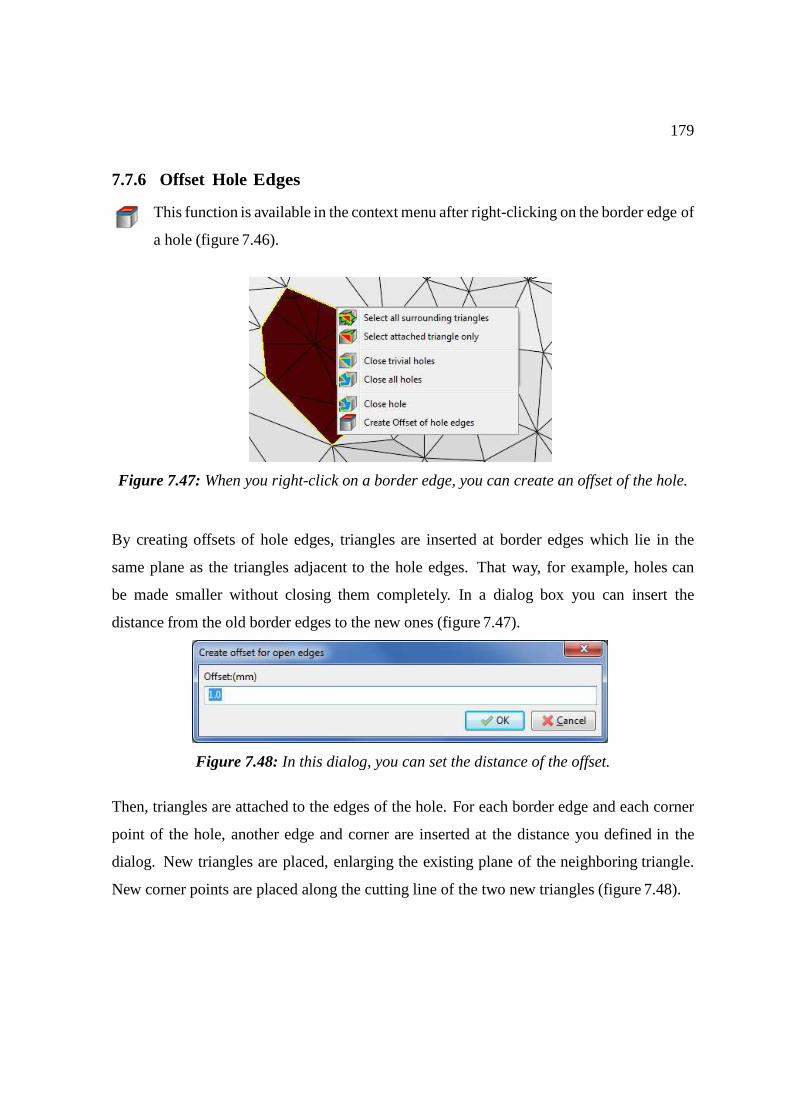
179
7.7.6 Offset Hole Edges
This function is available in the context menu after right-clicking on the border edge of
a hole (figure 7.46).
Figure 7.47: When you right-click on a border edge, you can create an offset of the hole.
By creating offsets of hole edges, triangles are inserted at border edges which lie in the
same plane as the triangles adjacent to the hole edges. That way, for example, holes can
be made smaller without closing them completely. In a dialog box you can insert the
distance from the old border edges to the new ones (figure 7.47).
Figure 7.48: In this dialog, you can set the distance of the offset.
Then, triangles are attached to the edges of the hole. For each border edge and each corner
point of the hole, another edge and corner are inserted at the distance you defined in the
dialog. New triangles are placed, enlarging the existing plane of the neighboring triangle.
New corner points are placed along the cutting line of the two new triangles (figure 7.48).
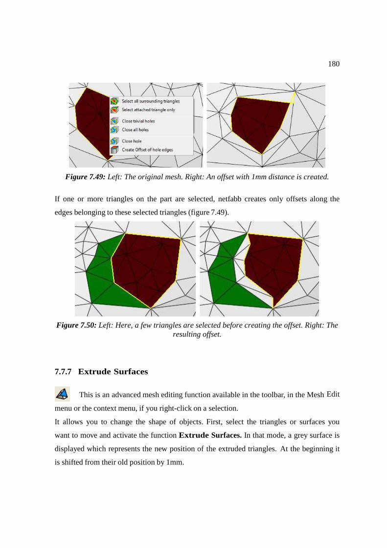
180
Figure 7.49: Left: The original mesh. Right: An offset with 1mm distance is created.
If one or more triangles on the part are selected, netfabb creates only offsets along the
edges belonging to these selected triangles (figure 7.49).
Figure 7.50: Left: Here, a few triangles are selected before creating the offset. Right: The resulting offset.
7.7.7 Extrude Surfaces
This is an advanced mesh editing function available in the toolbar, in the Mesh Edit
menu or the context menu, if you right-click on a selection.
It allows you to change the shape of objects. First, select the triangles or surfaces you
want to move and activate the function Extrude Surfaces. In that mode, a grey surface is
displayed which represents the new position of the extruded triangles. At the beginning it
is shifted from their old position by 1mm.
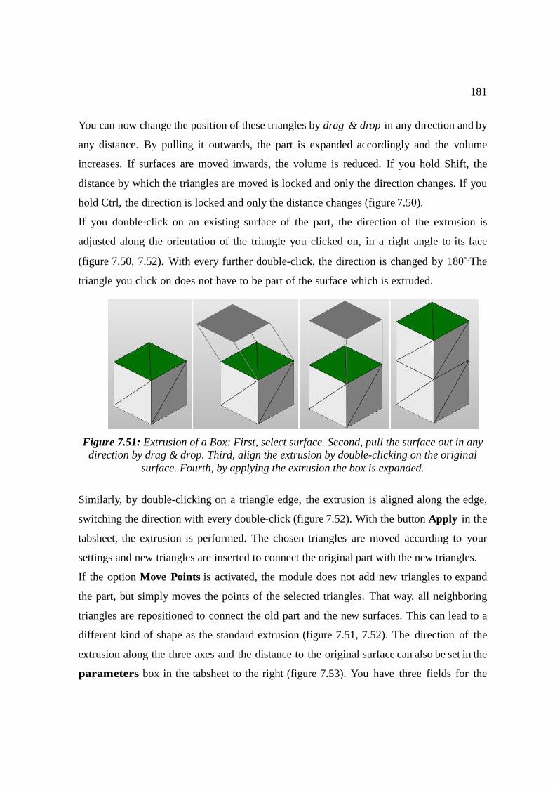
181
You can now change the position of these triangles by drag & drop in any direction and by
any distance. By pulling it outwards, the part is expanded accordingly and the volume
increases. If surfaces are moved inwards, the volume is reduced. If you hold Shift, the
distance by which the triangles are moved is locked and only the direction changes. If you
hold Ctrl, the direction is locked and only the distance changes (figure 7.50).
If you double-click on an existing surface of the part, the direction of the extrusion is
adjusted along the orientation of the triangle you clicked on, in a right angle to its face
(figure 7.50, 7.52). With every further double-click, the direction is changed by 180◦. The
triangle you click on does not have to be part of the surface which is extruded.
Figure 7.51: Extrusion of a Box: First, select surface. Second, pull the surface out in any direction by drag & drop. Third, align the extrusion by double-clicking on the original
surface. Fourth, by applying the extrusion the box is expanded.
Similarly, by double-clicking on a triangle edge, the extrusion is aligned along the edge,
switching the direction with every double-click (figure 7.52). With the button Apply in the
tabsheet, the extrusion is performed. The chosen triangles are moved according to your
settings and new triangles are inserted to connect the original part with the new triangles.
If the option Move Points is activated, the module does not add new triangles to expand
the part, but simply moves the points of the selected triangles. That way, all neighboring
triangles are repositioned to connect the old part and the new surfaces. This can lead to a
different kind of shape as the standard extrusion (figure 7.51, 7.52). The direction of the
extrusion along the three axes and the distance to the original surface can also be set in the
parameters box in the tabsheet to the right (figure 7.53). You have three fields for the
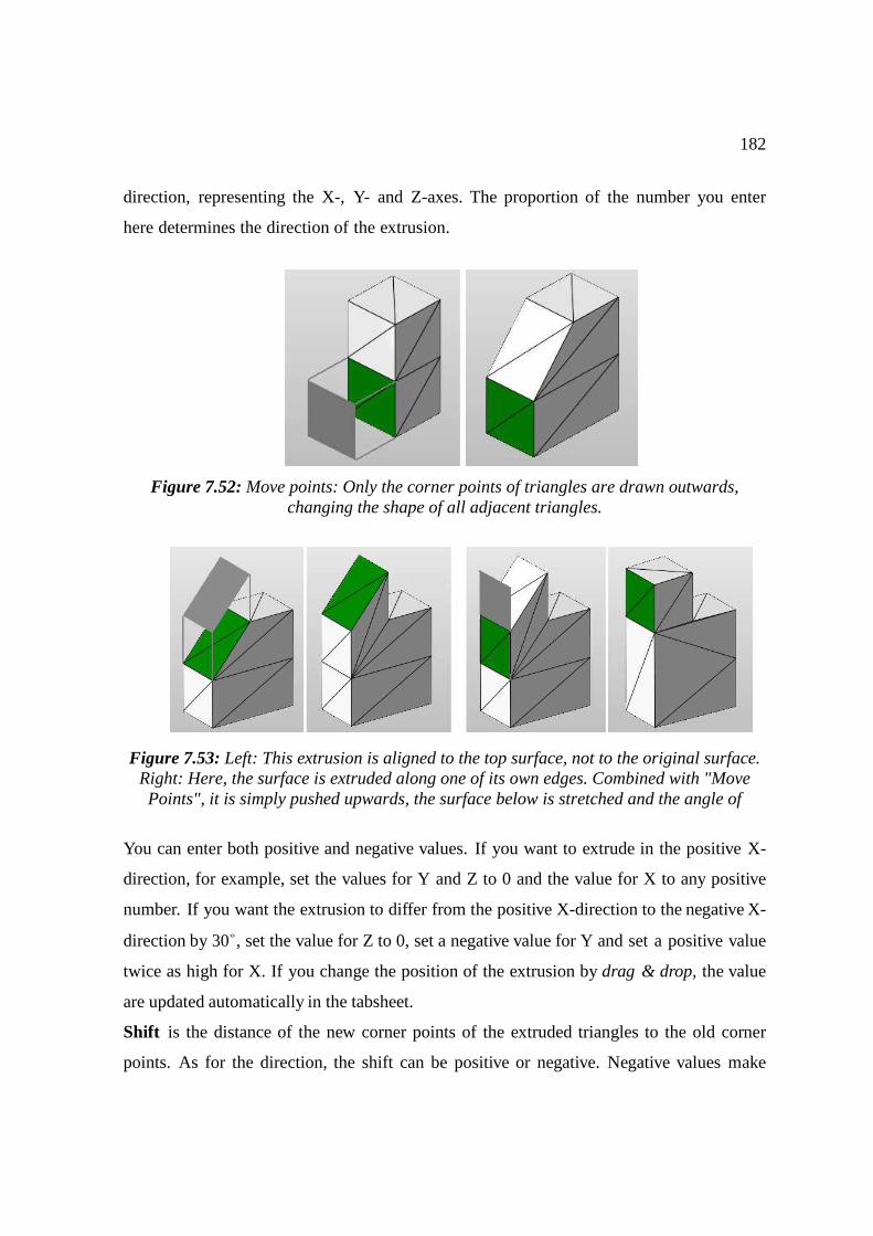
182
direction, representing the X-, Y- and Z-axes. The proportion of the number you enter
here determines the direction of the extrusion.
Figure 7.52: Move points: Only the corner points of triangles are drawn outwards, changing the shape of all adjacent triangles.
Figure 7.53: Left: This extrusion is aligned to the top surface, not to the original surface.
Right: Here, the surface is extruded along one of its own edges. Combined with "Move Points", it is simply pushed upwards, the surface below is stretched and the angle of
You can enter both positive and negative values. If you want to extrude in the positive X-
direction, for example, set the values for Y and Z to 0 and the value for X to any positive
number. If you want the extrusion to differ from the positive X-direction to the negative X-
direction by 30◦, set the value for Z to 0, set a negative value for Y and set a positive value
twice as high for X. If you change the position of the extrusion by drag & drop, the value
are updated automatically in the tabsheet.
Shift is the distance of the new corner points of the extruded triangles to the old corner
points. As for the direction, the shift can be positive or negative. Negative values make
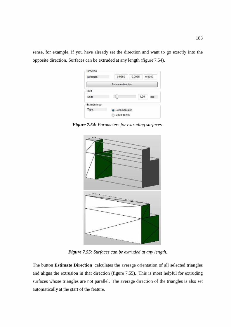
183
sense, for example, if you have already set the direction and want to go exactly into the
opposite direction. Surfaces can be extruded at any length (figure 7.54).
Figure 7.54: Parameters for extruding surfaces.
Figure 7.55: Surfaces can be extruded at any length.
The button Estimate Direction calculates the average orientation of all selected triangles
and aligns the extrusion in that direction (figure 7.55). This is most helpful for extruding
surfaces whose triangles are not parallel. The average direction of the triangles is also set
automatically at the start of the feature.
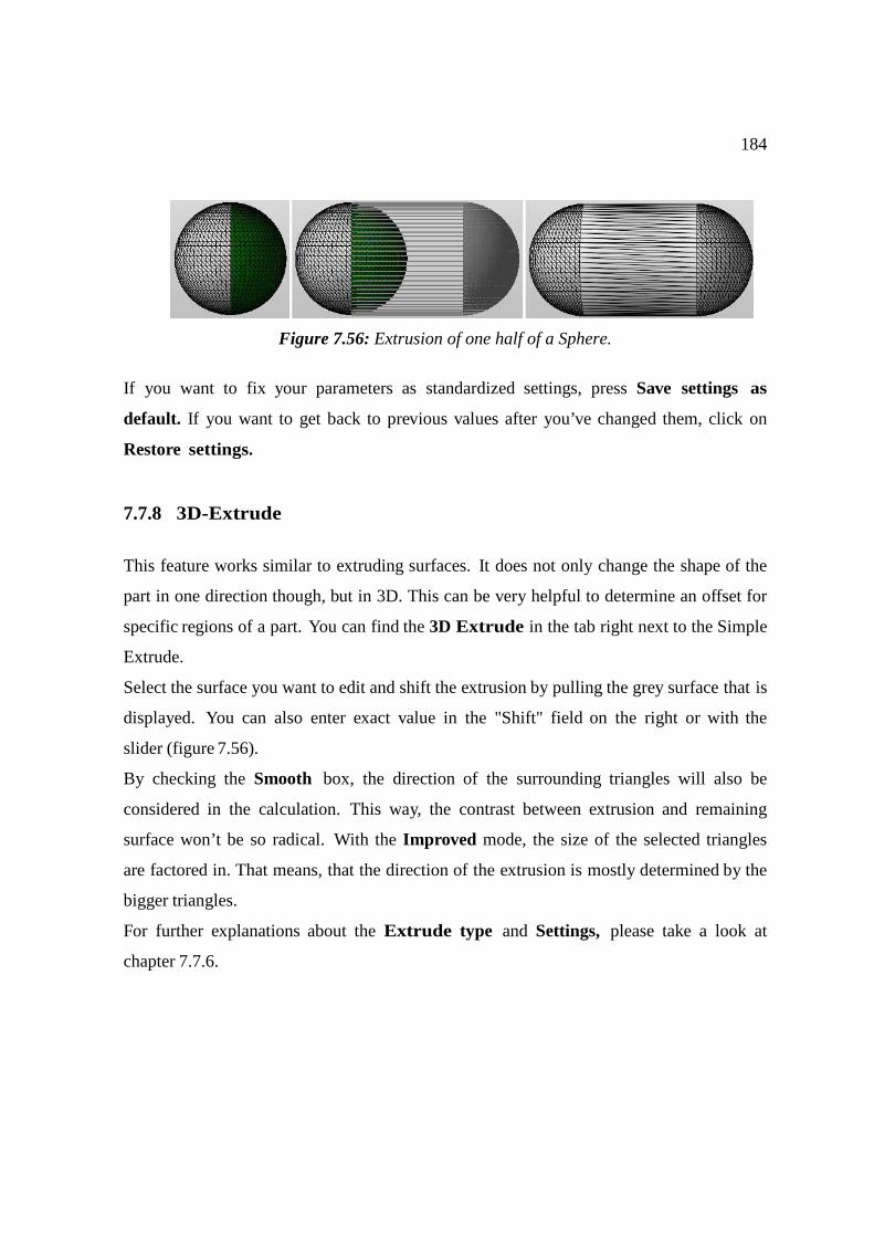
184
Figure 7.56: Extrusion of one half of a Sphere.
If you want to fix your parameters as standardized settings, press Save settings as
default. If you want to get back to previous values after you’ve changed them, click on
Restore settings.
7.7.8 3D-Extrude
This feature works similar to extruding surfaces. It does not only change the shape of the
part in one direction though, but in 3D. This can be very helpful to determine an offset for
specific regions of a part. You can find the 3D Extrude in the tab right next to the Simple
Extrude.
Select the surface you want to edit and shift the extrusion by pulling the grey surface that is
displayed. You can also enter exact value in the "Shift" field on the right or with the
slider (figure 7.56).
By checking the Smooth box, the direction of the surrounding triangles will also be
considered in the calculation. This way, the contrast between extrusion and remaining
surface won’t be so radical. With the Improved mode, the size of the selected triangles
are factored in. That means, that the direction of the extrusion is mostly determined by the
bigger triangles.
For further explanations about the Extrude type and Settings, please take a look at
chapter 7.7.6.
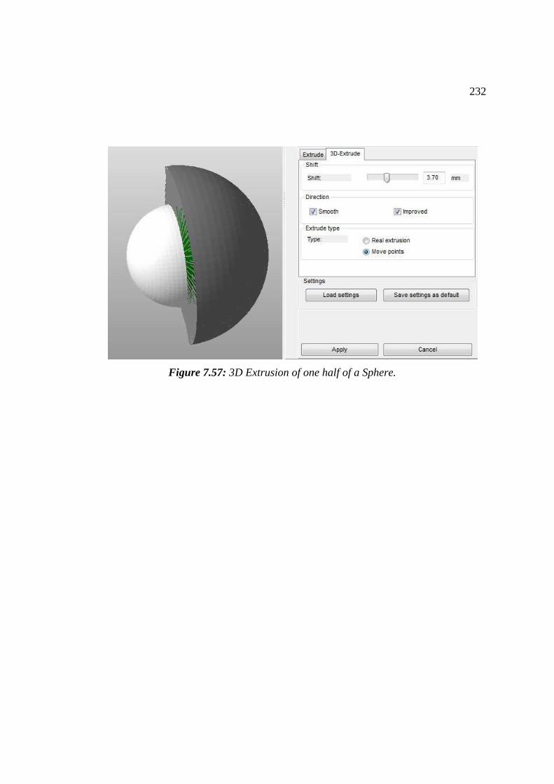
232
Figure 7.57: 3D Extrusion of one half of a Sphere.

233
8 Support Structures (Professional / Enterprise Add-on)
With netfabb’s Support Structure Module you can create support structures for
various 3D printing machines. There are two different products: DLP Support
Structures and the Enhanced Support Structures. They are both extra Add-ons for
netfabb Professional. In this manual, it’ll first be described what both tools have in
common (General settings and Downskin analysis) and then split up to DLP Module in
chapter 3 and to the Enhance Module in chapter 4.
Both support tools can be opened in the Extras menu, in the context menu, and in the
toolbar by clicking the according icon.
Figure 8.0: Example screenshot of a bar support structure.
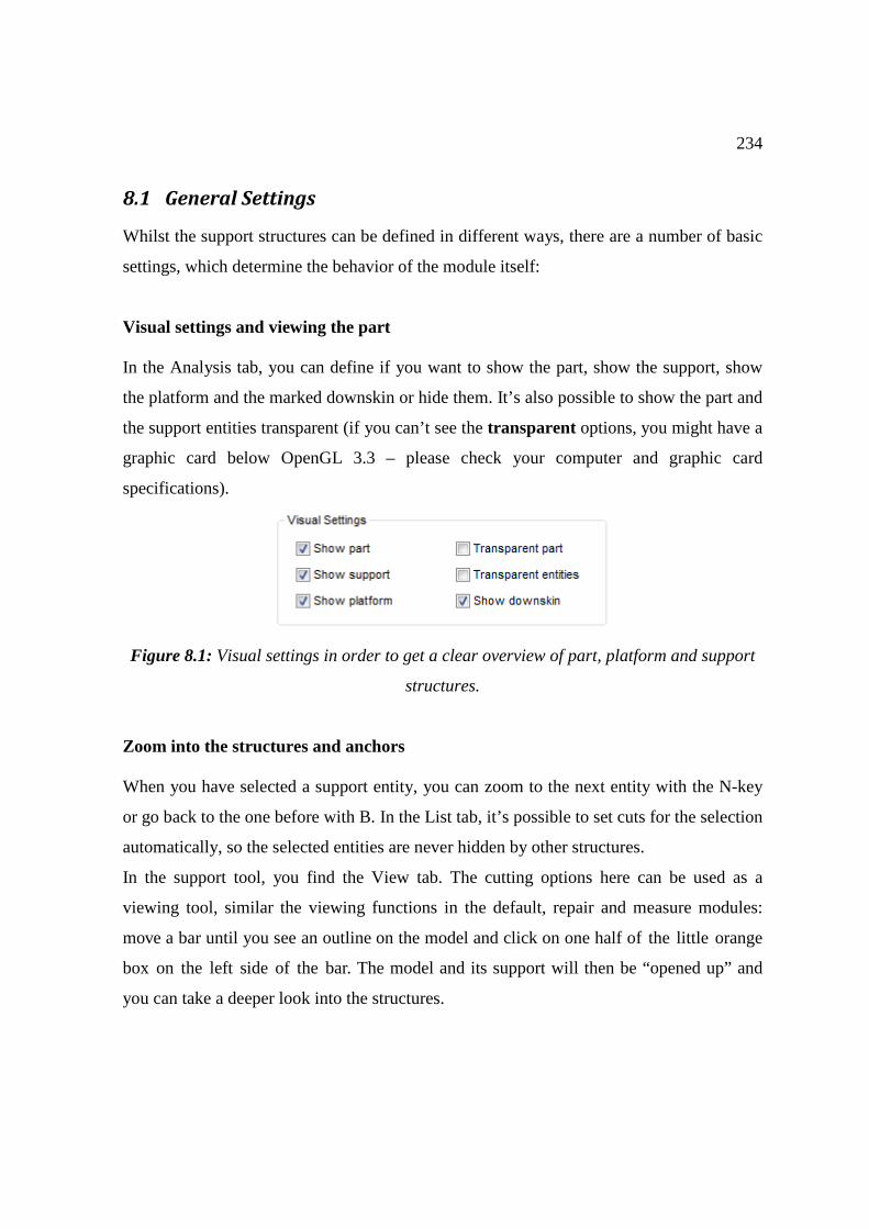
234
8.1 General Settings
Whilst the support structures can be defined in different ways, there are a number of basic
settings, which determine the behavior of the module itself:
Visual settings and viewing the part
In the Analysis tab, you can define if you want to show the part, show the support, show
the platform and the marked downskin or hide them. It’s also possible to show the part and
the support entities transparent (if you can’t see the transparent options, you might have a
graphic card below OpenGL 3.3 – please check your computer and graphic card
specifications).
Figure 8.1: Visual settings in order to get a clear overview of part, platform and support
structures.
Zoom into the structures and anchors
When you have selected a support entity, you can zoom to the next entity with the N-key
or go back to the one before with B. In the List tab, it’s possible to set cuts for the selection
automatically, so the selected entities are never hidden by other structures.
In the support tool, you find the View tab. The cutting options here can be used as a
viewing tool, similar the viewing functions in the default, repair and measure modules:
move a bar until you see an outline on the model and click on one half of the little orange
box on the left side of the bar. The model and its support will then be “opened up” and
you can take a deeper look into the structures.
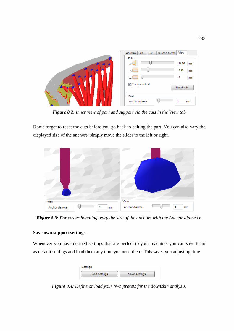
235
Figure 8.2: inner view of part and support via the cuts in the View tab
Don’t forget to reset the cuts before you go back to editing the part. You can also vary the
displayed size of the anchors: simply move the slider to the left or right.
Figure 8.3: For easier handling, vary the size of the anchors with the Anchor diameter.
Save own support settings
Whenever you have defined settings that are perfect to your machine, you can save them
as default settings and load them any time you need them. This saves you adjusting time.
Figure 8.4: Define or load your own presets for the downskin analysis.
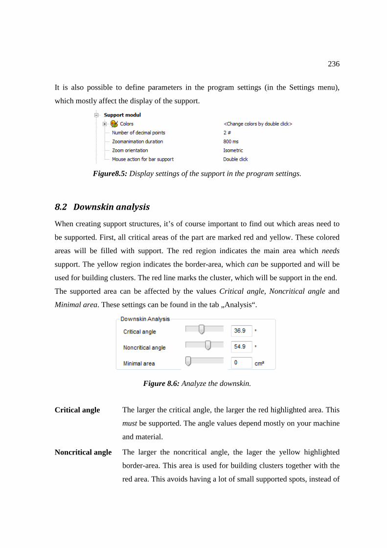
236
It is also possible to define parameters in the program settings (in the Settings menu),
which mostly affect the display of the support.
Figure8.5: Display settings of the support in the program settings.
8.2 Downskin analysis
When creating support structures, it’s of course important to find out which areas need to
be supported. First, all critical areas of the part are marked red and yellow. These colored
areas will be filled with support. The red region indicates the main area which needs
support. The yellow region indicates the border-area, which can be supported and will be
used for building clusters. The red line marks the cluster, which will be support in the end.
The supported area can be affected by the values Critical angle, Noncritical angle and
Minimal area. These settings can be found in the tab „Analysis“.
Figure 8.6: Analyze the downskin.
Critical angle The larger the critical angle, the larger the red highlighted area. This
must be supported. The angle values depend mostly on your machine
and material.
Noncritical angle The larger the noncritical angle, the lager the yellow highlighted
border-area. This area is used for building clusters together with the
red area. This avoids having a lot of small supported spots, instead of
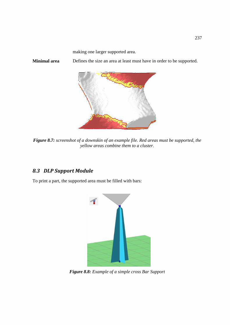
237
making one larger supported area.
Minimal area Defines the size an area at least must have in order to be supported.
Figure 8.7: screenshot of a downskin of an example file. Red areas must be supported, the yellow areas combine them to a cluster.
8.3 DLP Support Module
To print a part, the supported area must be filled with bars:
Figure 8.8: Example of a simple cross Bar Support

238
8.3.1 Manual Support Creation
8.3.1.1 Set anchors
The support is not connected directly with the part. It's connected from the floor up to an
anchor-point, which is located on the part. If a support-mode is selected, anchor-points can
be
moved,
or F9, created,
or F10, and deleted.
In the context menu of an anchor, you can either project it vertically up or down (it will be
placed on the platform or on the part), project it directly on the platform or remove all
unused anchors.
Figure 8.9: The anchor context menu for projecting or removing an anchors.
8.3.1.2 Create a bar manually
To create a bar simply choose the according icon (or press F6) and double click on
the surface you want to support. A vertical bar will be projected downwards. It’s also
possible to set a new anchor (F9) and project it up/down in order to create a bar
afterwards. To create a Bar Support, at least two anchor-points are needed.
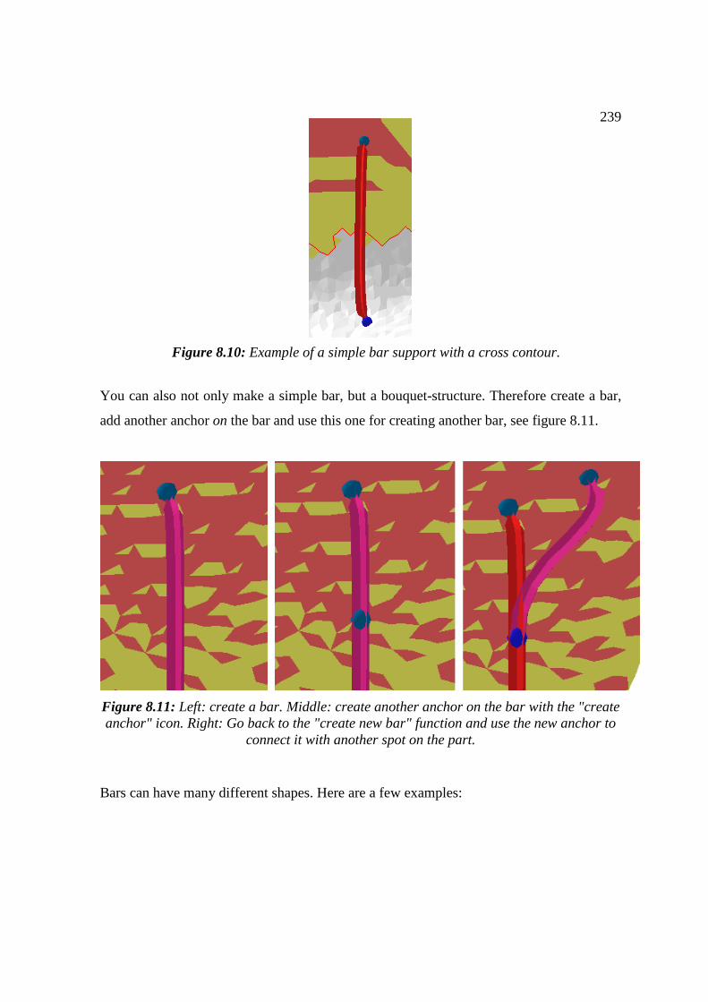
239
Figure 8.10: Example of a simple bar support with a cross contour.
You can also not only make a simple bar, but a bouquet-structure. Therefore create a bar,
add another anchor on the bar and use this one for creating another bar, see figure 8.11.
Figure 8.11: Left: create a bar. Middle: create another anchor on the bar with the "create anchor" icon. Right: Go back to the "create new bar" function and use the new anchor to
connect it with another spot on the part.
Bars can have many different shapes. Here are a few examples:
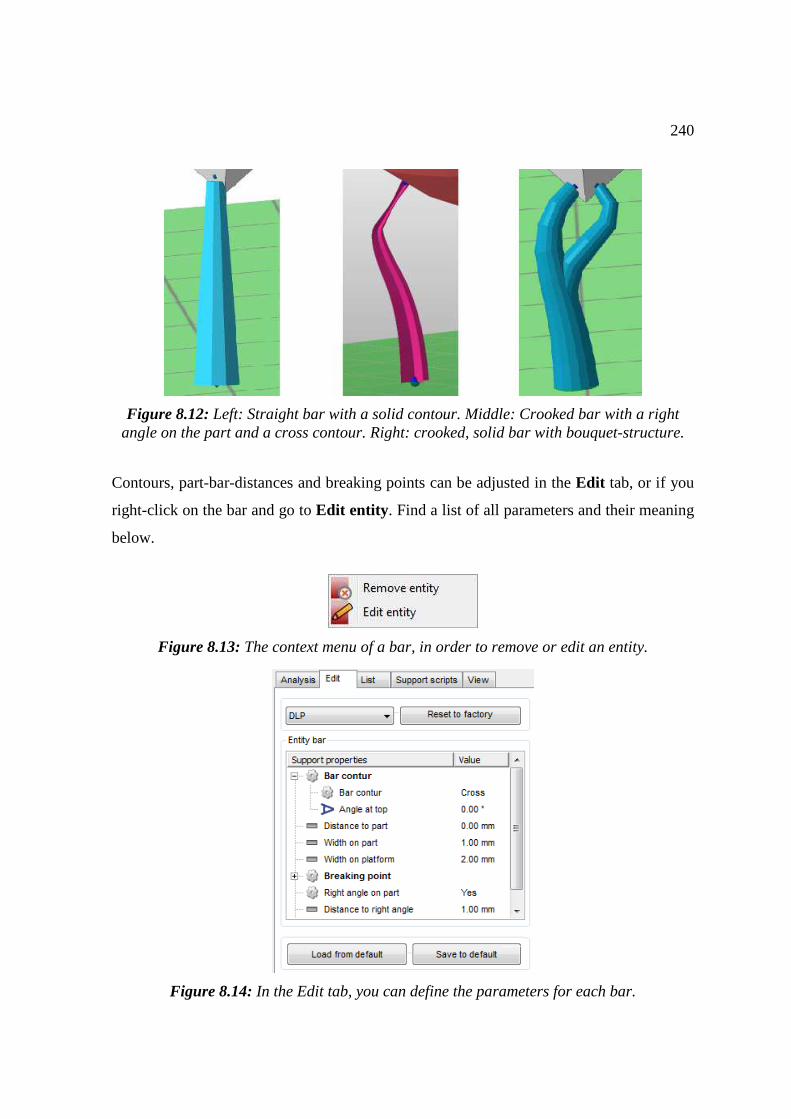
240
Figure 8.12: Left: Straight bar with a solid contour. Middle: Crooked bar with a right angle on the part and a cross contour. Right: crooked, solid bar with bouquet-structure.
Contours, part-bar-distances and breaking points can be adjusted in the Edit tab, or if you
right-click on the bar and go to Edit entity. Find a list of all parameters and their meaning
below.
Figure 8.13: The context menu of a bar, in order to remove or edit an entity.
Figure 8.14: In the Edit tab, you can define the parameters for each bar.
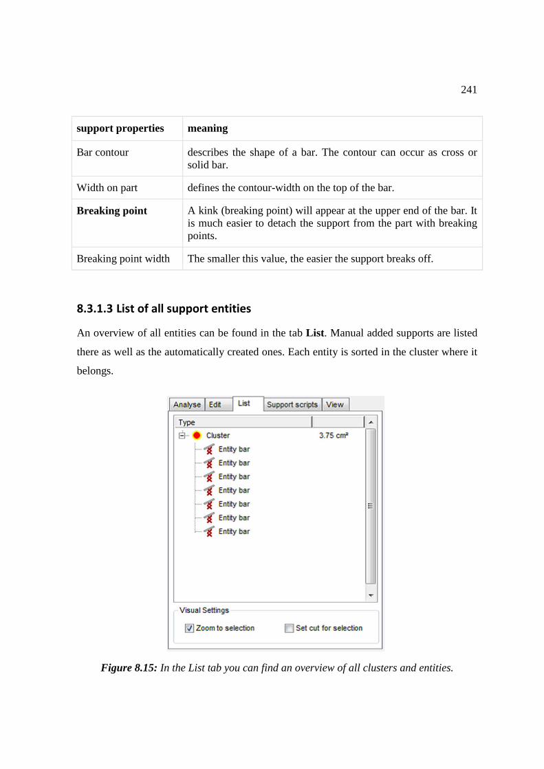
241
support properties meaning
Bar contour describes the shape of a bar. The contour can occur as cross or solid bar.
Width on part defines the contour-width on the top of the bar.
Breaking point A kink (breaking point) will appear at the upper end of the bar. It is much easier to detach the support from the part with breaking points.
Breaking point width The smaller this value, the easier the support breaks off.
8.3.1.3 List of all support entities
An overview of all entities can be found in the tab List. Manual added supports are listed
there as well as the automatically created ones. Each entity is sorted in the cluster where it
belongs.
Figure 8.15: In the List tab you can find an overview of all clusters and entities.
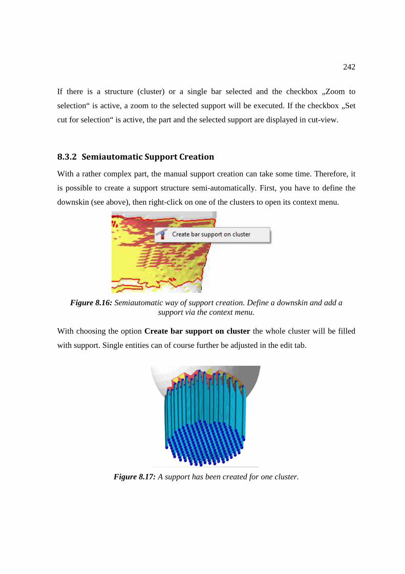
242
If there is a structure (cluster) or a single bar selected and the checkbox „Zoom to
selection“ is active, a zoom to the selected support will be executed. If the checkbox „Set
cut for selection“ is active, the part and the selected support are displayed in cut-view.
8.3.2 Semiautomatic Support Creation
With a rather complex part, the manual support creation can take some time. Therefore, it
is possible to create a support structure semi-automatically. First, you have to define the
downskin (see above), then right-click on one of the clusters to open its context menu.
Figure 8.16: Semiautomatic way of support creation. Define a downskin and add a support via the context menu.
With choosing the option Create bar support on cluster the whole cluster will be filled
with support. Single entities can of course further be adjusted in the edit tab.
Figure 8.17: A support has been created for one cluster.
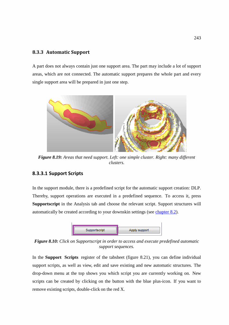
243
8.3.3 Automatic Support
A part does not always contain just one support area. The part may include a lot of support
areas, which are not connected. The automatic support prepares the whole part and every
single support area will be prepared in just one step.
Figure 8.19: Areas that need support. Left: one simple cluster. Right: many different clusters.
8.3.3.1 Support Scripts
In the support module, there is a predefined script for the automatic support creation: DLP.
Thereby, support operations are executed in a predefined sequence. To access it, press
Supportscript in the Analysis tab and choose the relevant script. Support structures will
automatically be created according to your downskin settings (see chapter 8.2).
Figure 8.10: Click on Supportscript in order to access and execute predefined automatic support sequences.
In the Support Scripts register of the tabsheet (figure 8.21), you can define individual
support scripts, as well as view, edit and save existing and new automatic structures. The
drop-down menu at the top shows you which script you are currently working on. New
scripts can be created by clicking on the button with the blue plus-icon. If you want to
remove existing scripts, double-click on the red X.
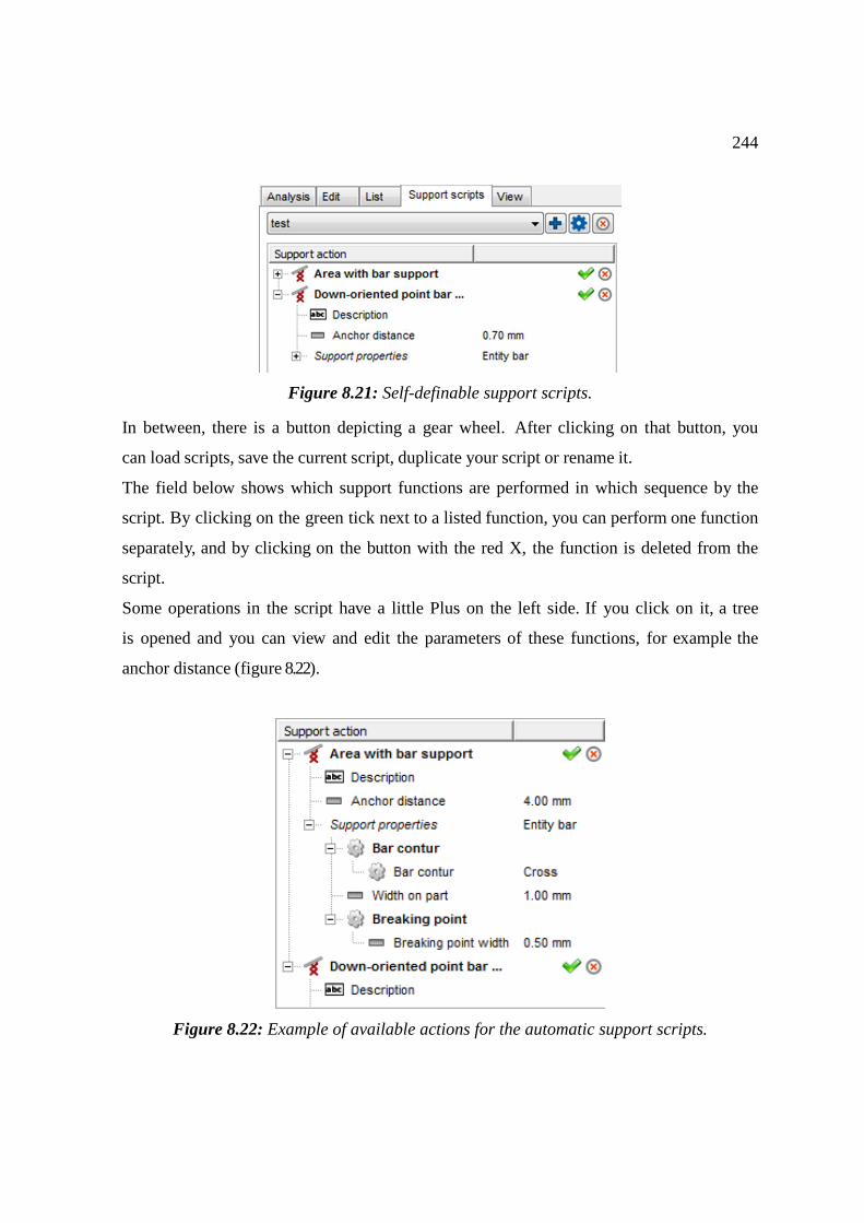
244
Figure 8.21: Self-definable support scripts.
In between, there is a button depicting a gear wheel. After clicking on that button, you
can load scripts, save the current script, duplicate your script or rename it.
The field below shows which support functions are performed in which sequence by the
script. By clicking on the green tick next to a listed function, you can perform one function
separately, and by clicking on the button with the red X, the function is deleted from the
script.
Some operations in the script have a little Plus on the left side. If you click on it, a tree
is opened and you can view and edit the parameters of these functions, for example the
anchor distance (figure 8.22).
Figure 8.22: Example of available actions for the automatic support scripts.
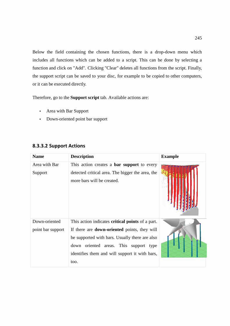
245
Below the field containing the chosen functions, there is a drop-down menu which
includes all functions which can be added to a script. This can be done by selecting a
function and click on "Add". Clicking "Clear" deletes all functions from the script. Finally,
the support script can be saved to your disc, for example to be copied to other computers,
or it can be executed directly.
Therefore, go to the Support script tab. Available actions are:
• Area with Bar Support
• Down-oriented point bar support
8.3.3.2 Support Actions
Name Description Example
Area with Bar
Support
This action creates a bar support to every
detected critical area. The bigger the area, the
more bars will be created.
Down-oriented
point bar support
This action indicates critical points of a part.
If there are down-oriented points, they will
be supported with bars. Usually there are also
down oriented areas. This support type
identifies them and will support it with bars,
too.
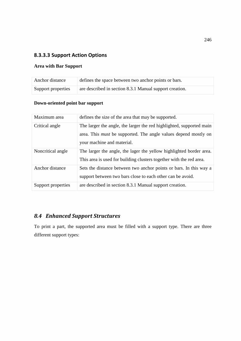
246
8.3.3.3 Support Action Options
Area with Bar Support
Anchor distance defines the space between two anchor points or bars.
Support properties are described in section 8.3.1 Manual support creation.
Down-oriented point bar support
Maximum area defines the size of the area that may be supported.
Critical angle The larger the angle, the larger the red highlighted, supported main
area. This must be supported. The angle values depend mostly on
your machine and material.
Noncritical angle The larger the angle, the lager the yellow highlighted border area.
This area is used for building clusters together with the red area.
Anchor distance Sets the distance between two anchor points or bars. In this way a
support between two bars close to each other can be avoid.
Support properties are described in section 8.3.1 Manual support creation.
8.4 Enhanced Support Structures
To print a part, the supported area must be filled with a support type. There are three
different support types:
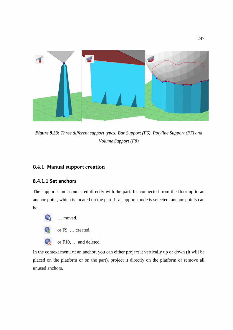
247
Figure 8.23: Three different support types: Bar Support (F6), Polyline Support (F7) and
Volume Support (F8)
8.4.1 Manual support creation
8.4.1.1 Set anchors
The support is not connected directly with the part. It's connected from the floor up to an
anchor-point, which is located on the part. If a support-mode is selected, anchor-points can
be …
… moved,
or F9, … created,
or F10, … and deleted.
In the context menu of an anchor, you can either project it vertically up or down (it will be
placed on the platform or on the part), project it directly on the platform or remove all
unused anchors.
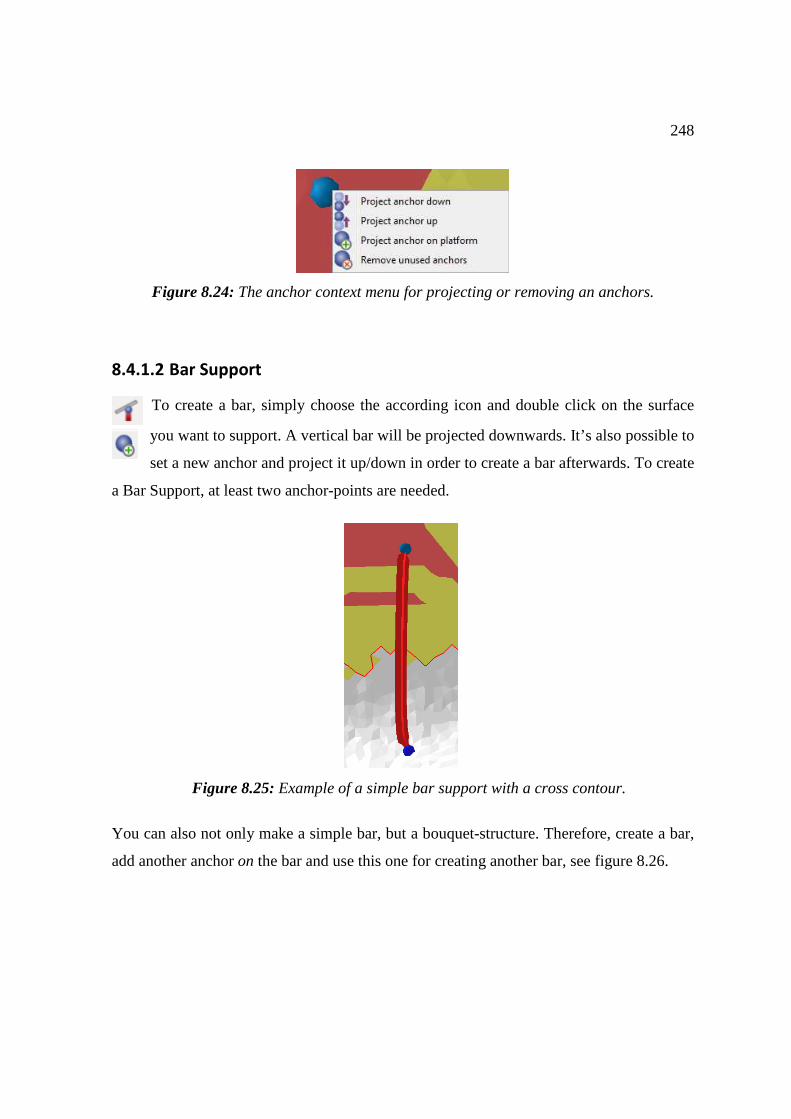
248
Figure 8.25: Example of a simple bar support with a cross contour.
Figure 8.24: The anchor context menu for projecting or removing an anchors.
8.4.1.2 Bar Support
To create a bar, simply choose the according icon and double click on the surface
you want to support. A vertical bar will be projected downwards. It’s also possible to
set a new anchor and project it up/down in order to create a bar afterwards. To create
a Bar Support, at least two anchor-points are needed.
You can also not only make a simple bar, but a bouquet-structure. Therefore, create a bar,
add another anchor on the bar and use this one for creating another bar, see figure 8.26.
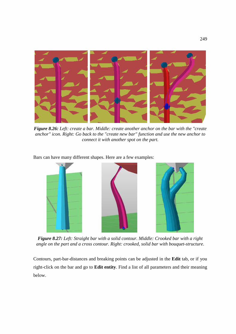
249
Figure 8.26: Left: create a bar. Middle: create another anchor on the bar with the "create anchor" icon. Right: Go back to the "create new bar" function and use the new anchor to
connect it with another spot on the part.
Bars can have many different shapes. Here are a few examples:
Figure 8.27: Left: Straight bar with a solid contour. Middle: Crooked bar with a right angle on the part and a cross contour. Right: crooked, solid bar with bouquet-structure.
Contours, part-bar-distances and breaking points can be adjusted in the Edit tab, or if you
right-click on the bar and go to Edit entity. Find a list of all parameters and their meaning
below.
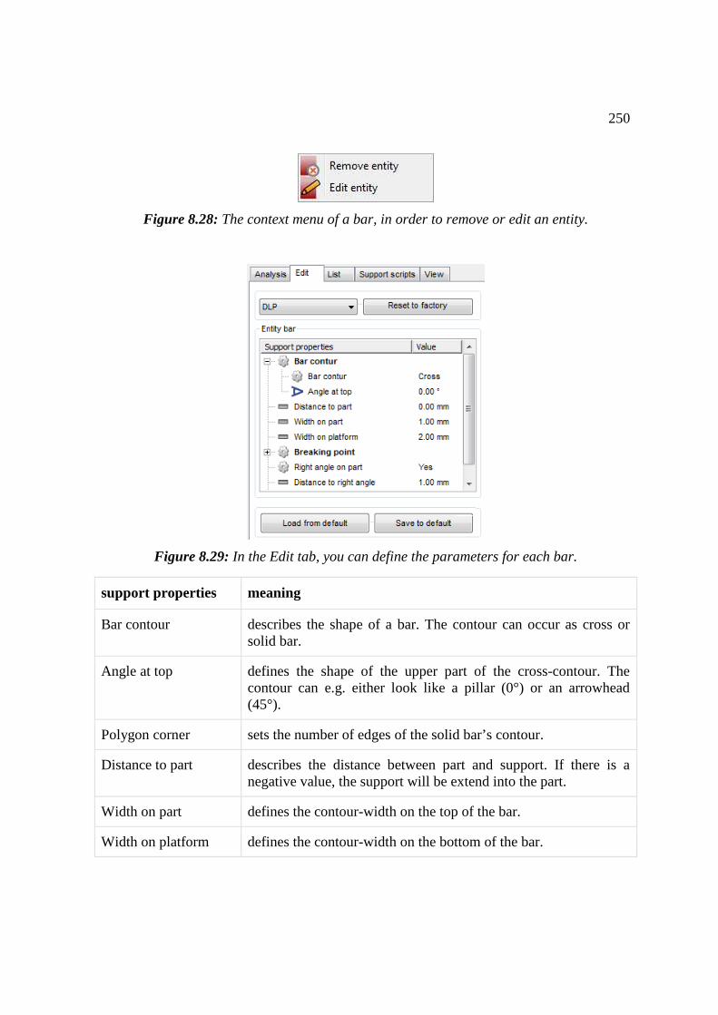
250
Figure 8.28: The context menu of a bar, in order to remove or edit an entity.
Figure 8.29: In the Edit tab, you can define the parameters for each bar.
support properties meaning
Bar contour describes the shape of a bar. The contour can occur as cross or solid bar.
Angle at top defines the shape of the upper part of the cross-contour. The contour can e.g. either look like a pillar (0°) or an arrowhead (45°).
Polygon corner sets the number of edges of the solid bar’s contour.
Distance to part describes the distance between part and support. If there is a negative value, the support will be extend into the part.
Width on part defines the contour-width on the top of the bar.
Width on platform defines the contour-width on the bottom of the bar.
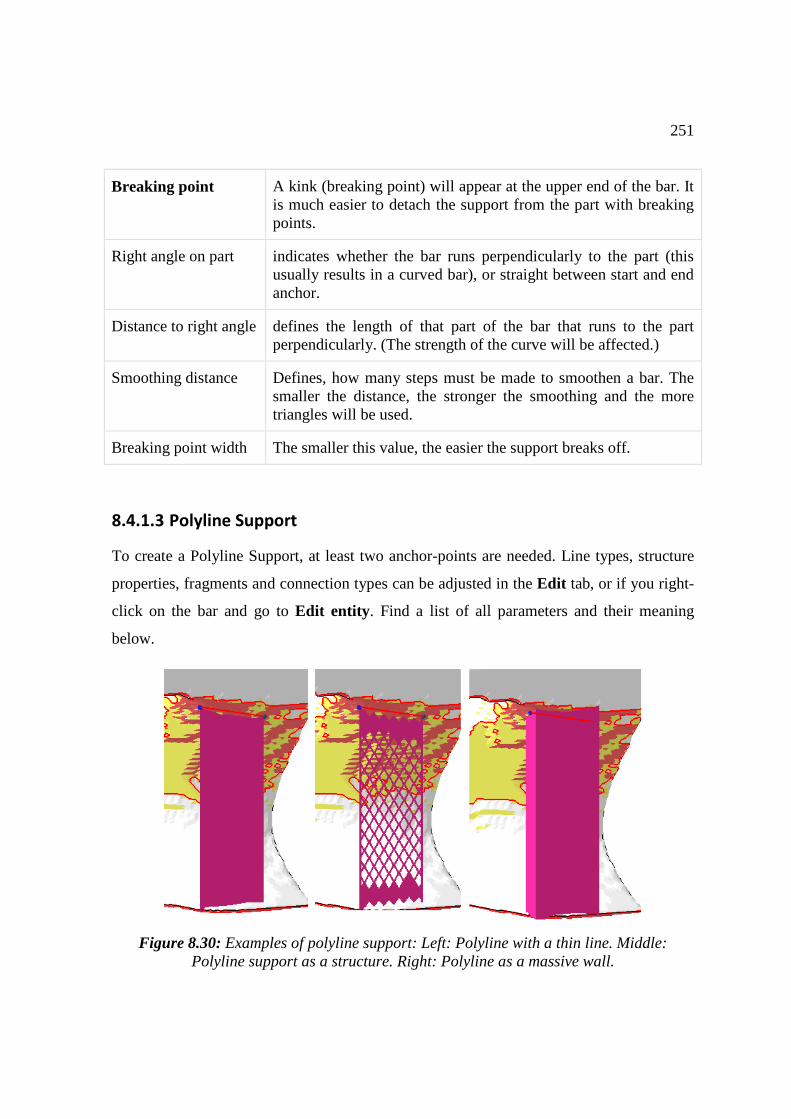
251
Breaking point A kink (breaking point) will appear at the upper end of the bar. It is much easier to detach the support from the part with breaking points.
Right angle on part
indicates whether the bar runs perpendicularly to the part (this usually results in a curved bar), or straight between start and end anchor.
Distance to right angle defines the length of that part of the bar that runs to the part perpendicularly. (The strength of the curve will be affected.)
Smoothing distance Defines, how many steps must be made to smoothen a bar. The smaller the distance, the stronger the smoothing and the more triangles will be used.
Breaking point width The smaller this value, the easier the support breaks off.
8.4.1.3 Polyline Support
To create a Polyline Support, at least two anchor-points are needed. Line types, structure
properties, fragments and connection types can be adjusted in the Edit tab, or if you right-
click on the bar and go to Edit entity. Find a list of all parameters and their meaning
below.
Figure 8.30: Examples of polyline support: Left: Polyline with a thin line. Middle: Polyline support as a structure. Right: Polyline as a massive wall.
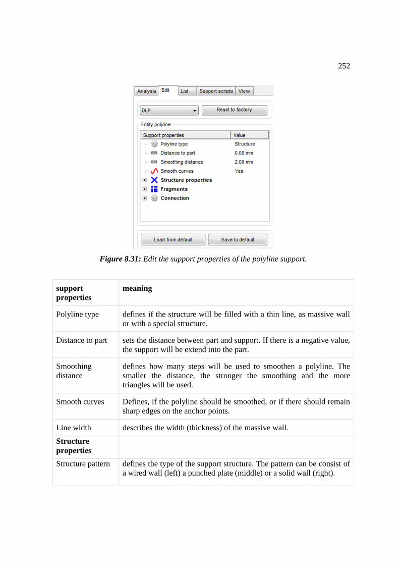
252
Figure 8.31: Edit the support properties of the polyline support.
support properties
meaning
Polyline type defines if the structure will be filled with a thin line, as massive wall or with a special structure.
Distance to part sets the distance between part and support. If there is a negative value, the support will be extend into the part.
Smoothing distance
defines how many steps will be used to smoothen a polyline. The smaller the distance, the stronger the smoothing and the more triangles will be used.
Smooth curves Defines, if the polyline should be smoothed, or if there should remain sharp edges on the anchor points.
Line width describes the width (thickness) of the massive wall.
Structure properties
Structure pattern defines the type of the support structure. The pattern can be consist of a wired wall (left) a punched plate (middle) or a solid wall (right).
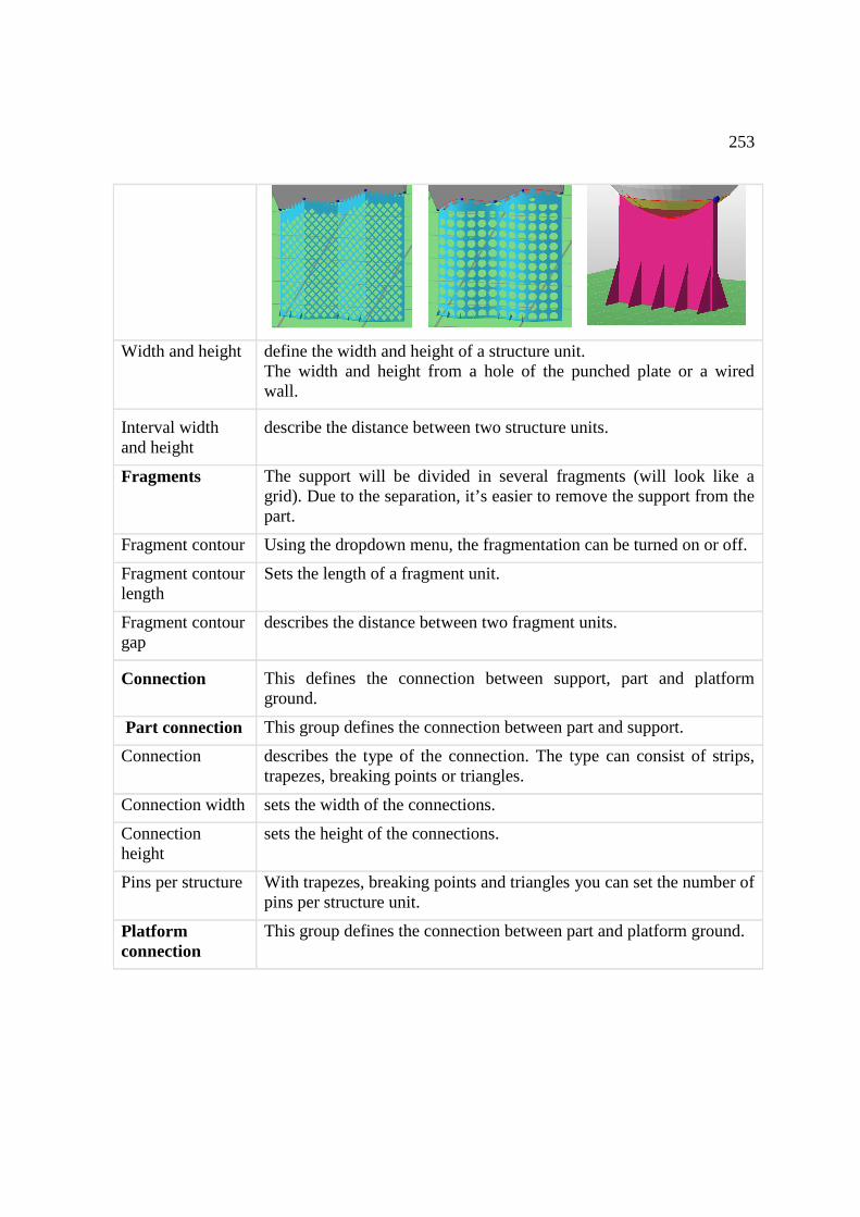
253
Width and height define the width and height of a structure unit. The width and height from a hole of the punched plate or a wired wall.
Interval width and height
describe the distance between two structure units.
Fragments The support will be divided in several fragments (will look like a grid). Due to the separation, it’s easier to remove the support from the part.
Fragment contour Using the dropdown menu, the fragmentation can be turned on or off.
Fragment contour length
Sets the length of a fragment unit.
Fragment contour gap
describes the distance between two fragment units.
Connection This defines the connection between support, part and platform ground.
Part connection This group defines the connection between part and support.
Connection describes the type of the connection. The type can consist of strips, trapezes, breaking points or triangles.
Connection width sets the width of the connections.
Connection height
sets the height of the connections.
Pins per structure With trapezes, breaking points and triangles you can set the number of pins per structure unit.
Platform connection
This group defines the connection between part and platform ground.
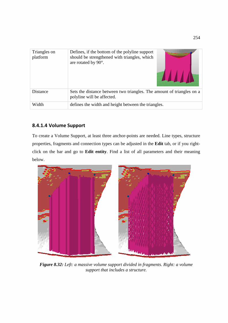
254
Triangles on platform
Defines, if the bottom of the polyline support should be strengthened with triangles, which are rotated by 90°.
Distance Sets the distance between two triangles. The amount of triangles on a polyline will be affected.
Width defines the width and height between the triangles.
8.4.1.4 Volume Support
To create a Volume Support, at least three anchor-points are needed. Line types, structure
properties, fragments and connection types can be adjusted in the Edit tab, or if you right-
click on the bar and go to Edit entity. Find a list of all parameters and their meaning
below.
Figure 8.32: Left: a massive volume support divided in fragments. Right: a volume support that includes a structure.
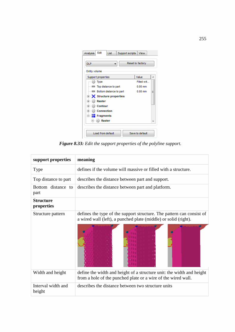
255
Figure 8.33: Edit the support properties of the polyline support.
support properties meaning
Type defines if the volume will massive or filled with a structure.
Top distance to part describes the distance between part and support.
Bottom distance to part
describes the distance between part and platform.
Structure properties
Structure pattern defines the type of the support structure. The pattern can consist of a wired wall (left), a punched plate (middle) or solid (right).
Width and height define the width and height of a structure unit: the width and height from a hole of the punched plate or a wire of the wired wall.
Interval width and height
describes the distance between two structure units
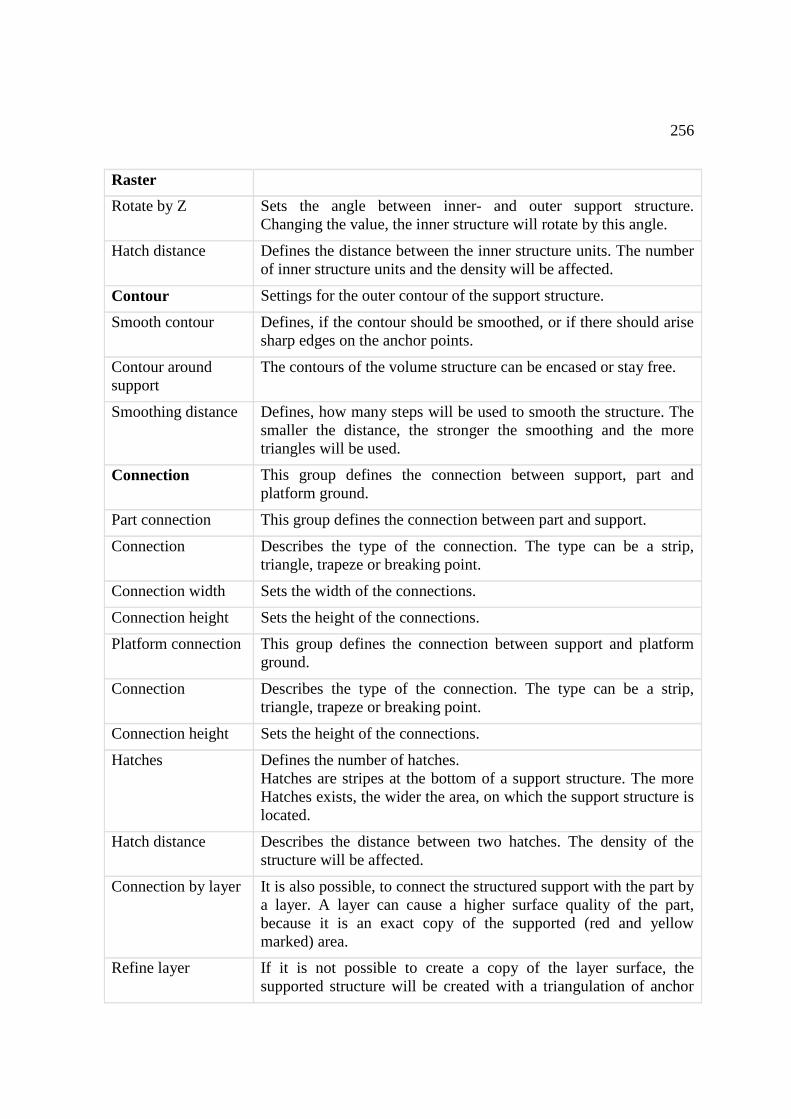
256
Raster
Rotate by Z Sets the angle between inner- and outer support structure. Changing the value, the inner structure will rotate by this angle.
Hatch distance Defines the distance between the inner structure units. The number of inner structure units and the density will be affected.
Contour Settings for the outer contour of the support structure.
Smooth contour Defines, if the contour should be smoothed, or if there should arise sharp edges on the anchor points.
Contour around support
The contours of the volume structure can be encased or stay free.
Smoothing distance Defines, how many steps will be used to smooth the structure. The smaller the distance, the stronger the smoothing and the more triangles will be used.
Connection This group defines the connection between support, part and platform ground.
Part connection This group defines the connection between part and support.
Connection Describes the type of the connection. The type can be a strip, triangle, trapeze or breaking point.
Connection width Sets the width of the connections.
Connection height Sets the height of the connections.
Platform connection This group defines the connection between support and platform ground.
Connection Describes the type of the connection. The type can be a strip, triangle, trapeze or breaking point.
Connection height Sets the height of the connections.
Hatches Defines the number of hatches. Hatches are stripes at the bottom of a support structure. The more Hatches exists, the wider the area, on which the support structure is located.
Hatch distance Describes the distance between two hatches. The density of the structure will be affected.
Connection by layer It is also possible, to connect the structured support with the part by a layer. A layer can cause a higher surface quality of the part, because it is an exact copy of the supported (red and yellow marked) area.
Refine layer If it is not possible to create a copy of the layer surface, the supported structure will be created with a triangulation of anchor
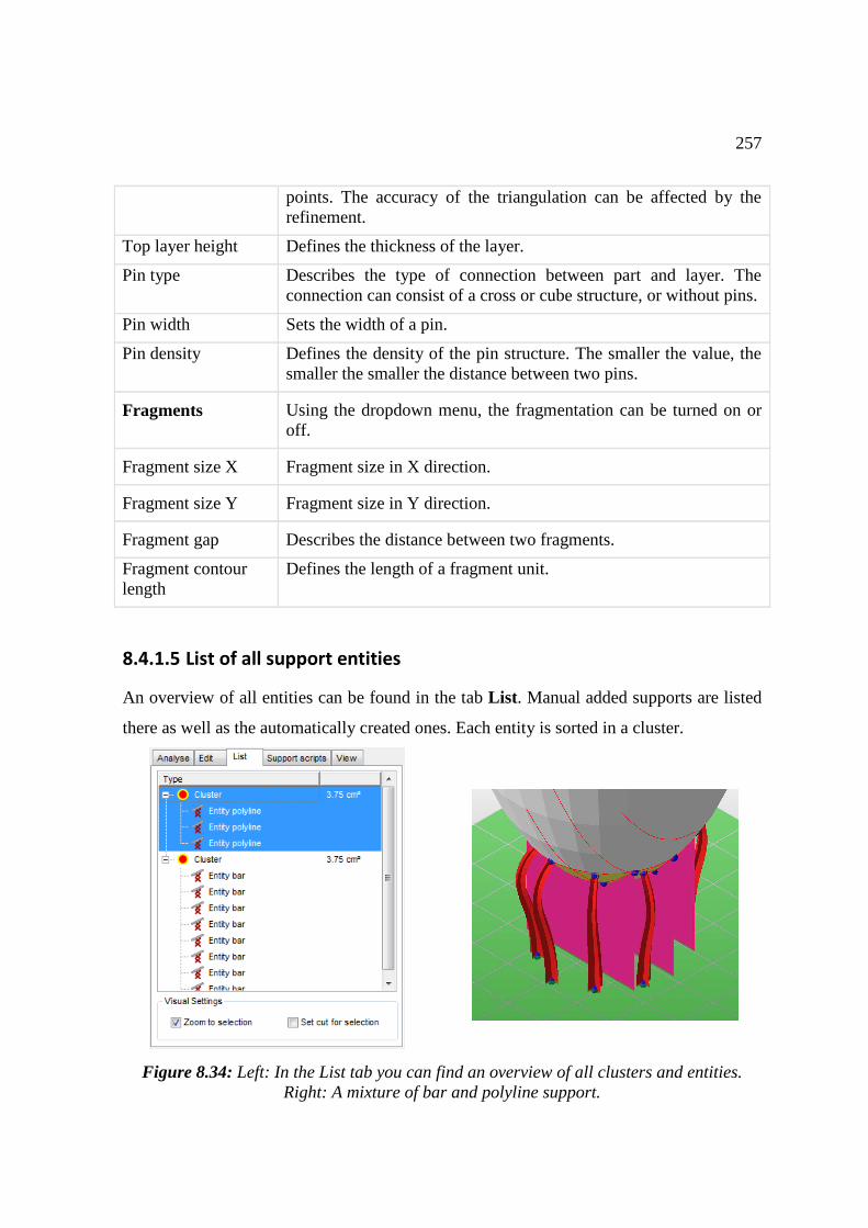
257
points. The accuracy of the triangulation can be affected by the refinement.
Top layer height Defines the thickness of the layer.
Pin type Describes the type of connection between part and layer. The connection can consist of a cross or cube structure, or without pins.
Pin width Sets the width of a pin.
Pin density Defines the density of the pin structure. The smaller the value, the smaller the smaller the distance between two pins.
Fragments Using the dropdown menu, the fragmentation can be turned on or off.
Fragment size X Fragment size in X direction.
Fragment size Y Fragment size in Y direction.
Fragment gap Describes the distance between two fragments.
Fragment contour length
Defines the length of a fragment unit.
8.4.1.5 List of all support entities
An overview of all entities can be found in the tab List. Manual added supports are listed
there as well as the automatically created ones. Each entity is sorted in a cluster.
Figure 8.34: Left: In the List tab you can find an overview of all clusters and entities. Right: A mixture of bar and polyline support.
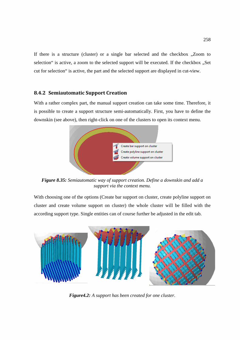
258
If there is a structure (cluster) or a single bar selected and the checkbox „Zoom to
selection“ is active, a zoom to the selected support will be executed. If the checkbox „Set
cut for selection“ is active, the part and the selected support are displayed in cut-view.
8.4.2 Semiautomatic Support Creation
With a rather complex part, the manual support creation can take some time. Therefore, it
is possible to create a support structure semi-automatically. First, you have to define the
downskin (see above), then right-click on one of the clusters to open its context menu.
Figure 8.35: Semiautomatic way of support creation. Define a downskin and add a support via the context menu.
With choosing one of the options (Create bar support on cluster, create polyline support on
cluster and create volume support on cluster) the whole cluster will be filled with the
according support type. Single entities can of course further be adjusted in the edit tab.
Figure4.2: A support has been created for one cluster.
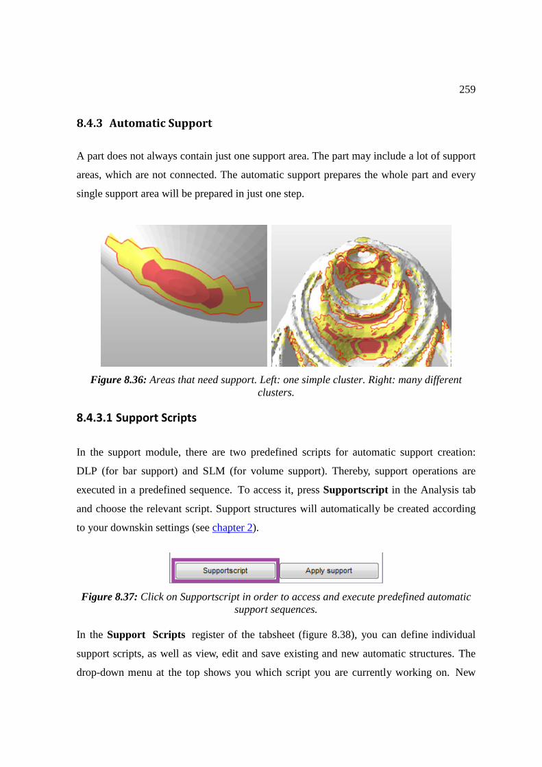
259
8.4.3 Automatic Support
A part does not always contain just one support area. The part may include a lot of support
areas, which are not connected. The automatic support prepares the whole part and every
single support area will be prepared in just one step.
Figure 8.36: Areas that need support. Left: one simple cluster. Right: many different clusters.
8.4.3.1 Support Scripts
In the support module, there are two predefined scripts for automatic support creation:
DLP (for bar support) and SLM (for volume support). Thereby, support operations are
executed in a predefined sequence. To access it, press Supportscript in the Analysis tab
and choose the relevant script. Support structures will automatically be created according
to your downskin settings (see chapter 2).
Figure 8.37: Click on Supportscript in order to access and execute predefined automatic support sequences.
In the Support Scripts register of the tabsheet (figure 8.38), you can define individual
support scripts, as well as view, edit and save existing and new automatic structures. The
drop-down menu at the top shows you which script you are currently working on. New
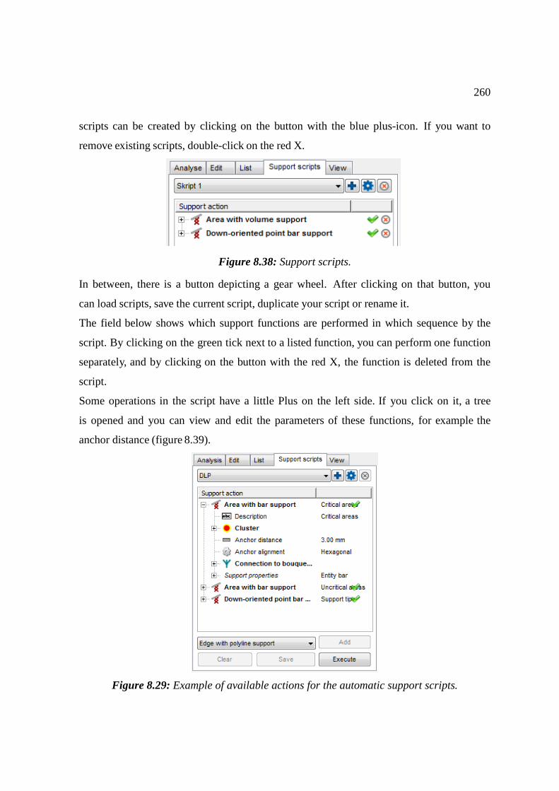
260
scripts can be created by clicking on the button with the blue plus-icon. If you want to
remove existing scripts, double-click on the red X.
Figure 8.38: Support scripts.
In between, there is a button depicting a gear wheel. After clicking on that button, you
can load scripts, save the current script, duplicate your script or rename it.
The field below shows which support functions are performed in which sequence by the
script. By clicking on the green tick next to a listed function, you can perform one function
separately, and by clicking on the button with the red X, the function is deleted from the
script.
Some operations in the script have a little Plus on the left side. If you click on it, a tree
is opened and you can view and edit the parameters of these functions, for example the
anchor distance (figure 8.39).
Figure 8.29: Example of available actions for the automatic support scripts.
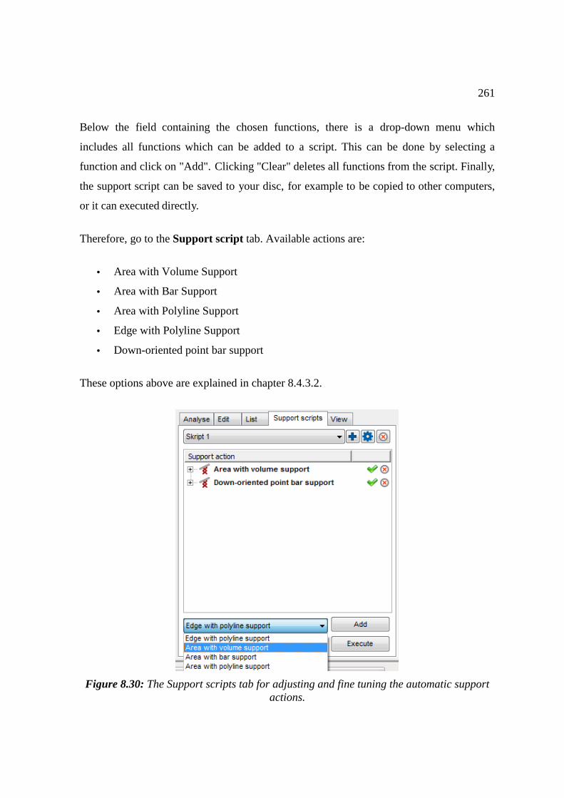
261
Below the field containing the chosen functions, there is a drop-down menu which
includes all functions which can be added to a script. This can be done by selecting a
function and click on "Add". Clicking "Clear" deletes all functions from the script. Finally,
the support script can be saved to your disc, for example to be copied to other computers,
or it can executed directly.
Therefore, go to the Support script tab. Available actions are:
• Area with Volume Support
• Area with Bar Support
• Area with Polyline Support
• Edge with Polyline Support
• Down-oriented point bar support
These options above are explained in chapter 8.4.3.2.
Figure 8.30: The Support scripts tab for adjusting and fine tuning the automatic support actions.

262
8.4.3.2 Support Actions
Name Description Example
Edge with
Polyline Support
This action indicates down oriented, critical
edges. The edges will be supported with
polylines.
Area with
Volume Support
This action creates a volume support to
every detected critical area. Anchor points
will be created around the contour of this
area.
Area with Bar
Support
This action creates a bar support to every
detected critical area. The bigger the area, the
more bars will be created.
Area with
Polyline Support
This action creates a polyline support to
every detected support area. The area will
supported with one parallel polyline after
another.

263
Down-oriented
point bar support
This action indicates critical points of a part.
If there are down-oriented points, they will
be supported with bars. Usually there are also
down oriented areas. This support type
identifies them and will support it with bars,
too.
Support Action Options
Cluster Detection
The (red and yellow marked) supported area of a part is called „Cluster“. For each area-
based automatic support action it is possible to define a cluster, on which the area support
will be applied.
Figure 8.41: Left: script with several support actions. Right: tree view of a cluster action.
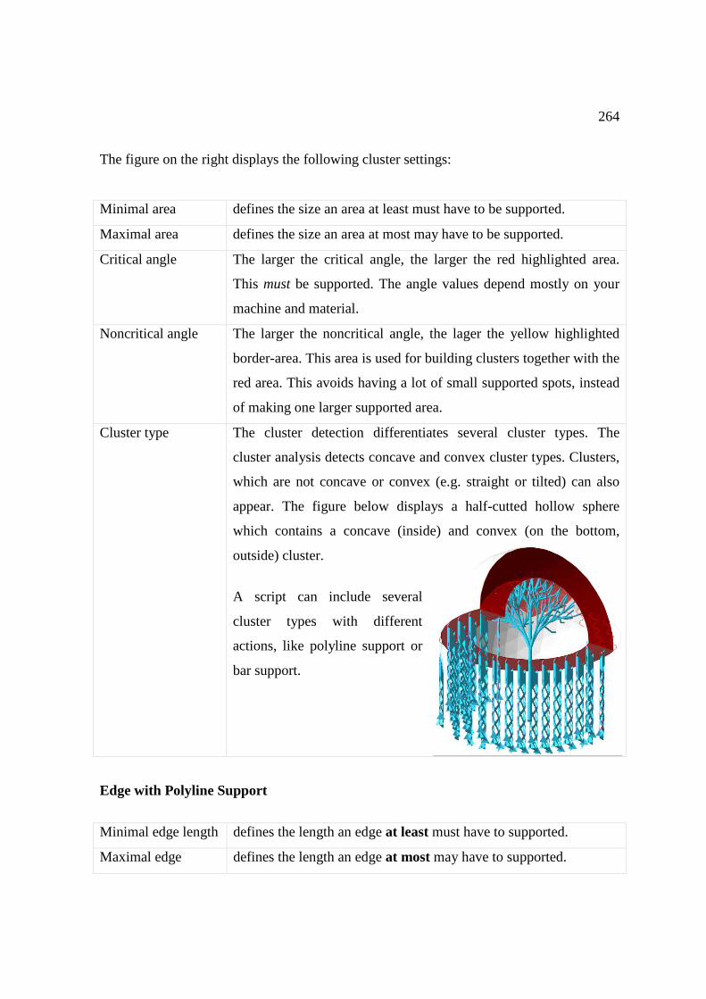
264
The figure on the right displays the following cluster settings:
Minimal area defines the size an area at least must have to be supported.
Maximal area defines the size an area at most may have to be supported.
Critical angle The larger the critical angle, the larger the red highlighted area.
This must be supported. The angle values depend mostly on your
machine and material.
Noncritical angle The larger the noncritical angle, the lager the yellow highlighted
border-area. This area is used for building clusters together with the
red area. This avoids having a lot of small supported spots, instead
of making one larger supported area.
Cluster type The cluster detection differentiates several cluster types. The
cluster analysis detects concave and convex cluster types. Clusters,
which are not concave or convex (e.g. straight or tilted) can also
appear. The figure below displays a half-cutted hollow sphere
which contains a concave (inside) and convex (on the bottom,
outside) cluster.
A script can include several
cluster types with different
actions, like polyline support or
bar support.
Edge with Polyline Support
Minimal edge length defines the length an edge at least must have to supported.
Maximal edge defines the length an edge at most may have to supported.
265
length
Maximal polyline
curvature
sets the curvature of a polyline may have at most. If this maximum
value will be passed, a new polyline begins.
Maximal edge angle
to XY-plane
describes the maximum angle between an edge and the XY-plane.
If the maximum angle will be passed, the edge is not detected.
Create anchor on
curvature
defines on which curvature of the edge a new anchor point will be
added. The anchor points will be created around the edge.
Anchor distance Sets the distance between two anchor points.
Contour offset Sets the distance between an anchor point and a clear area.
Support properties Are described in chapter 8.4.1.3 Polyline Support.
Area with Volume Support
Cluster See chapter 8.4.3.2 Cluster detection.
Anchor distance sets the distance between two anchor points. The anchor points will
be created around the contour of the supported area.
Create anchor on
curvature
Defines on which curvature of the edge a new anchor point will be
added. The anchor points will be created around the edge.
Contour offset to
wall
The anchor points along the contour can be moved further apart
from the edge. The offset describes the distance from the edge to
the next wall.
Free contour offset Describes the distance between an anchor point and the next edge.
Support properties Are described in section 8.4.1.4 Volume Support.
Area with Bar Support
Cluster See chapter 8.4.3.2 Cluster detection.
Anchor distance defines the space between two anchor points or bars.
Anchor alignment There are two ways to support the critical area with bar:
Rectangular means, that the support structure is arranged
266
rectangular to the area. Hexagonal means, that the structure is
arranged hexagonal, which enables to arrange more bars on the
same area.
Connection to
bouquet-structure
Not every bar has its start point at the bottom of a platform. It is
possible to create a branch of the bouquet-structure, which saves
time to construction and substance too, compare chapter 8.4.1.2
Bar support.
Diameter of
bouquet-structure
defines the maximum diameter of the whole bouquet-structure.
Height of bouquet-
structure
Describes the height between the first branch of the bouquet-
structure and the part.
Recursive depth of
bouquet-structure
Sets the limit of branches per bar between the first branch and the
part.
Support properties are described in section 8.4.1.2 Bar Support.
Area with Polyline Support
Cluster See chapter 8.4.3.2 Cluster detection.
Anchor distance The detected area will supported with polylines. The anchor
distance defines the space between two anchor points for each
polyline.
Hatch distance sets the distance between two polylines.
Rotate by Z Rotates the arrangement of the polylines by the entered value.
Wave amplitude Defines the distance between every intermediate anchor point from
a polyline. A value >0 creates a wave (if polyline is smoothed) or a
zig zag pattern. (if polyline is not smoothed)
Support properties are described in section 8.4.1.3 Polyline Support.
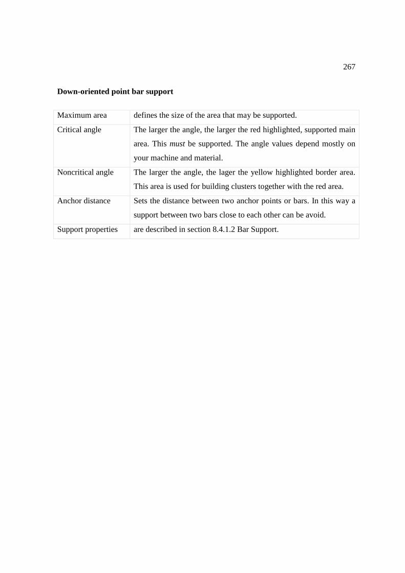
267
Down-oriented point bar support
Maximum area defines the size of the area that may be supported.
Critical angle The larger the angle, the larger the red highlighted, supported main
area. This must be supported. The angle values depend mostly on
your machine and material.
Noncritical angle The larger the angle, the lager the yellow highlighted border area.
This area is used for building clusters together with the red area.
Anchor distance Sets the distance between two anchor points or bars. In this way a
support between two bars close to each other can be avoid.
Support properties are described in section 8.4.1.2 Bar Support.

268
9 Measuring and Quality Assurance
9.1 The Measuring Tool
The measuring tool is activated by selecting a part and clicking on the measuring
icon in the toolbar or choosing New Measuring in the Extras menu or Extras
submenu of the context menu.
It allows the measurement of distances between points, edges and surfaces, as well as
radii and angles. It opens the measuring screen with the selected part only and provides
all measuring options in the tabsheet, where instructions are given and all measuring
results are specified in detail (figure 8.1). The options for changing perspectives and
zooming in the measuring screen are the same as in the main screen, only with less default
zoom options.
In the project tree, the measuring is integrated as subordinate directory of the part, with
single measuring operations as subordinate elements to that directory. After conducting
other operations, you can always return to the measurement by selecting it in the project
tree. If you right-click on the measuring in the project tree, you can rename it or remove it
(figure 8.2).
The measurements are performed by the setting of anchor points. It is possible to define
any number of measurement operations in the same screen and measuring. For a
subsequent quality test, it is also possible to set anchors in order to add notes. When a
measurement is conducted, a blue line (=arrow) appears between the anchors and the
result of the measurement is shown in a small box in the middle (figure 8.3). Also, a new
anchor is created in the center of the measurement, either in the middle of a distance or in the
center of a radius or at the apex of an angle. All anchors can be used again for subsequent
measurements (as in figure 8.12 and 8.15).
The box specifying the measured value represents a measuring point and, by drag &
drop, can be moved sideways together with the blue line into a parallel position. In that
case, the ends of the line are connected to the anchors by two more arrows, and the
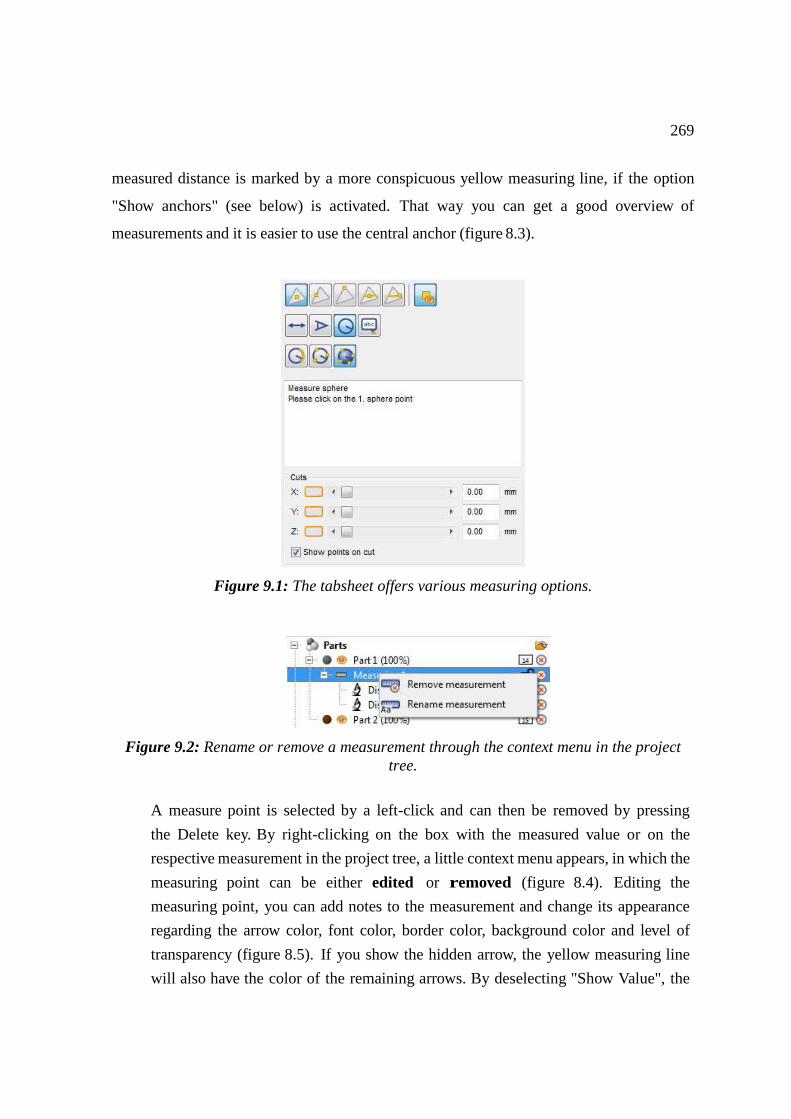
269
measured distance is marked by a more conspicuous yellow measuring line, if the option
"Show anchors" (see below) is activated. That way you can get a good overview of
measurements and it is easier to use the central anchor (figure 8.3).
Figure 9.1: The tabsheet offers various measuring options.
Figure 9.2: Rename or remove a measurement through the context menu in the project tree.
A measure point is selected by a left-click and can then be removed by pressing
the Delete key. By right-clicking on the box with the measured value or on the
respective measurement in the project tree, a little context menu appears, in which the
measuring point can be either edited or removed (figure 8.4). Editing the
measuring point, you can add notes to the measurement and change its appearance
regarding the arrow color, font color, border color, background color and level of
transparency (figure 8.5). If you show the hidden arrow, the yellow measuring line
will also have the color of the remaining arrows. By deselecting "Show Value", the
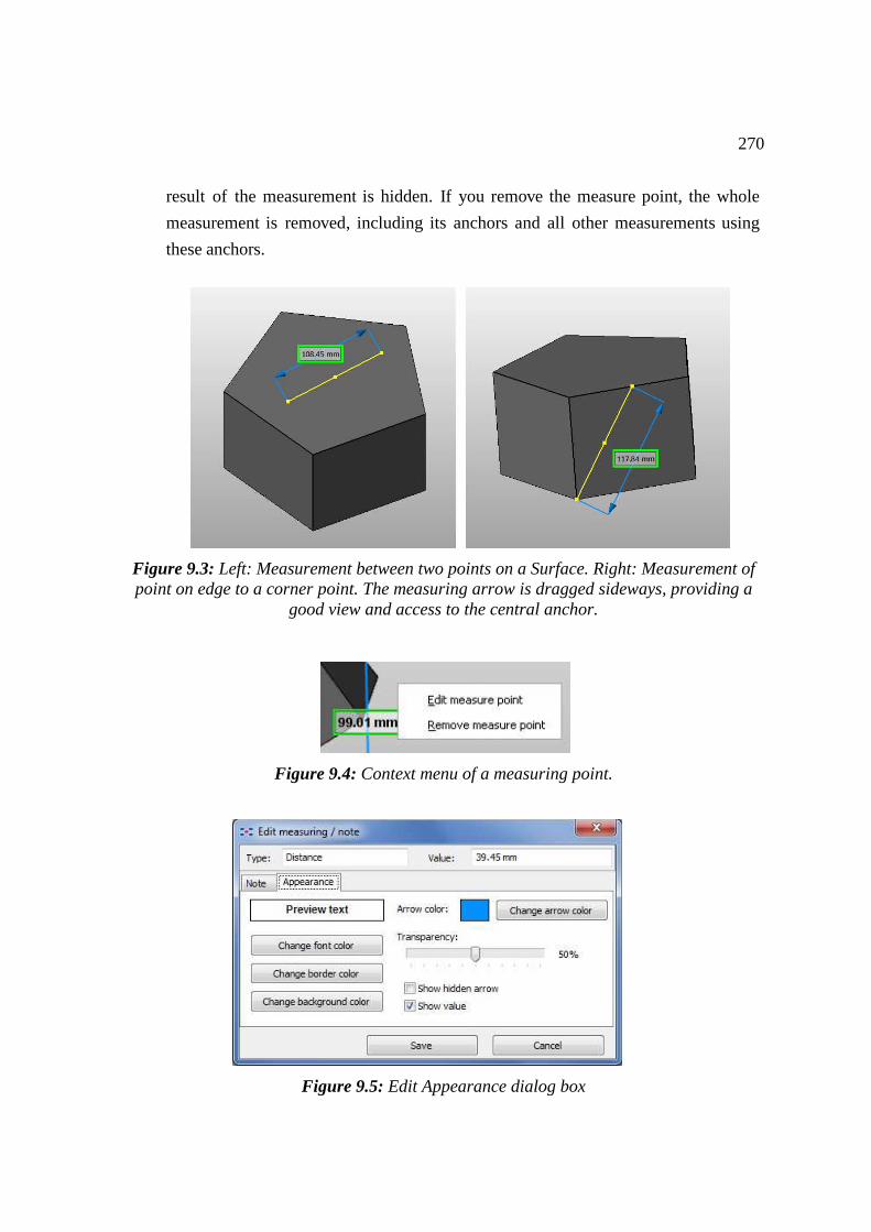
270
result of the measurement is hidden. If you remove the measure point, the whole
measurement is removed, including its anchors and all other measurements using
these anchors.
Figure 9.3: Left: Measurement between two points on a Surface. Right: Measurement of point on edge to a corner point. The measuring arrow is dragged sideways, providing a
good view and access to the central anchor.
Figure 9.4: Context menu of a measuring point.
Figure 9.5: Edit Appearance dialog box
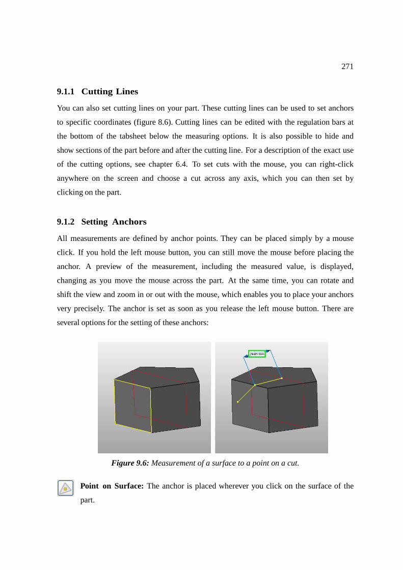
271
9.1.1 Cutting Lines
You can also set cutting lines on your part. These cutting lines can be used to set anchors
to specific coordinates (figure 8.6). Cutting lines can be edited with the regulation bars at
the bottom of the tabsheet below the measuring options. It is also possible to hide and
show sections of the part before and after the cutting line. For a description of the exact use
of the cutting options, see chapter 6.4. To set cuts with the mouse, you can right-click
anywhere on the screen and choose a cut across any axis, which you can then set by
clicking on the part.
9.1.2 Setting Anchors
All measurements are defined by anchor points. They can be placed simply by a mouse
click. If you hold the left mouse button, you can still move the mouse before placing the
anchor. A preview of the measurement, including the measured value, is displayed,
changing as you move the mouse across the part. At the same time, you can rotate and
shift the view and zoom in or out with the mouse, which enables you to place your anchors
very precisely. The anchor is set as soon as you release the left mouse button. There are
several options for the setting of these anchors:
Figure 9.6: Measurement of a surface to a point on a cut.
Point on Surface: The anchor is placed wherever you click on the surface of the
part.
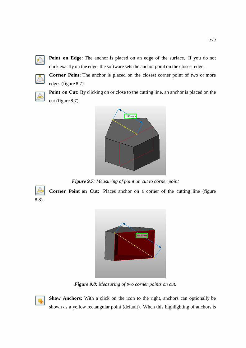
272
Point on Edge: The anchor is placed on an edge of the surface. If you do not
click exactly on the edge, the software sets the anchor point on the closest edge.
Corner Point: The anchor is placed on the closest corner point of two or more
edges (figure 8.7).
Point on Cut: By clicking on or close to the cutting line, an anchor is placed on the
cut (figure 8.7).
Figure 9.7: Measuring of point on cut to corner point
Corner Point on Cut: Places anchor on a corner of the cutting line (figure
8.8).
Figure 9.8: Measuring of two corner points on cut.
Show Anchors: With a click on the icon to the right, anchors can optionally be
shown as a yellow rectangular point (default). When this highlighting of anchors is
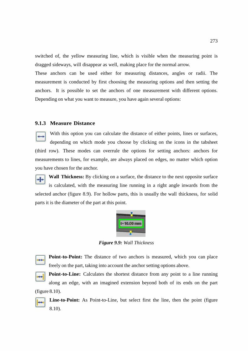
273
switched of, the yellow measuring line, which is visible when the measuring point is
dragged sideways, will disappear as well, making place for the normal arrow.
These anchors can be used either for measuring distances, angles or radii. The
measurement is conducted by first choosing the measuring options and then setting the
anchors. It is possible to set the anchors of one measurement with different options.
Depending on what you want to measure, you have again several options:
9.1.3 Measure Distance
With this option you can calculate the distance of either points, lines or surfaces,
depending on which mode you choose by clicking on the icons in the tabsheet
(third row). These modes can overrule the options for setting anchors: anchors for
measurements to lines, for example, are always placed on edges, no matter which option
you have chosen for the anchor.
Wall Thickness: By clicking on a surface, the distance to the next opposite surface
is calculated, with the measuring line running in a right angle inwards from the
selected anchor (figure 8.9). For hollow parts, this is usually the wall thickness, for solid
parts it is the diameter of the part at this point.
Figure 9.9: Wall Thickness
Point-to-Point: The distance of two anchors is measured, which you can place
freely on the part, taking into account the anchor setting options above.
Point-to-Line: Calculates the shortest distance from any point to a line running
along an edge, with an imagined extension beyond both of its ends on the part
(figure 8.10).
Line-to-Point: As Point-to-Line, but select first the line, then the point (figure
8.10).
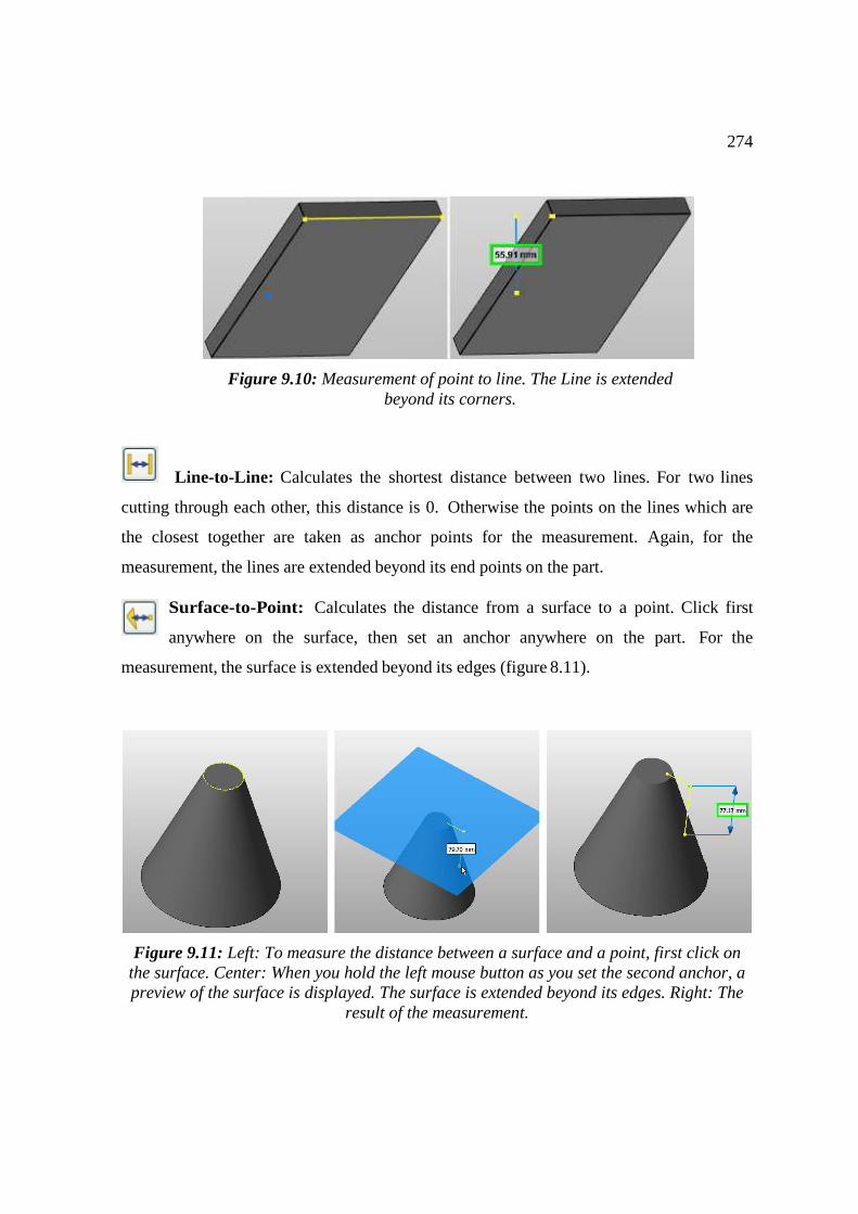
274
Line-to-Line: Calculates the shortest distance between two lines. For two lines
cutting through each other, this distance is 0. Otherwise the points on the lines which are
the closest together are taken as anchor points for the measurement. Again, for the
measurement, the lines are extended beyond its end points on the part.
Surface-to-Point: Calculates the distance from a surface to a point. Click first
anywhere on the surface, then set an anchor anywhere on the part. For the
measurement, the surface is extended beyond its edges (figure 8.11).
Figure 9.11: Left: To measure the distance between a surface and a point, first click on the surface. Center: When you hold the left mouse button as you set the second anchor, a preview of the surface is displayed. The surface is extended beyond its edges. Right: The
result of the measurement.
Figure 9.10: Measurement of point to line. The Line is extended beyond its corners.
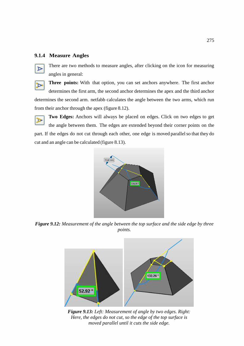
275
9.1.4 Measure Angles
There are two methods to measure angles, after clicking on the icon for measuring
angles in general:
Three points: With that option, you can set anchors anywhere. The first anchor
determines the first arm, the second anchor determines the apex and the third anchor
determines the second arm. netfabb calculates the angle between the two arms, which run
from their anchor through the apex (figure 8.12).
Two Edges: Anchors will always be placed on edges. Click on two edges to get
the angle between them. The edges are extended beyond their corner points on the
part. If the edges do not cut through each other, one edge is moved parallel so that they do
cut and an angle can be calculated (figure 8.13).
Figure 9.12: Measurement of the angle between the top surface and the side edge by three points.
Figure 9.13: Left: Measurement of angle by two edges. Right: Here, the edges do not cut, so the edge of the top surface is
moved parallel until it cuts the side edge.
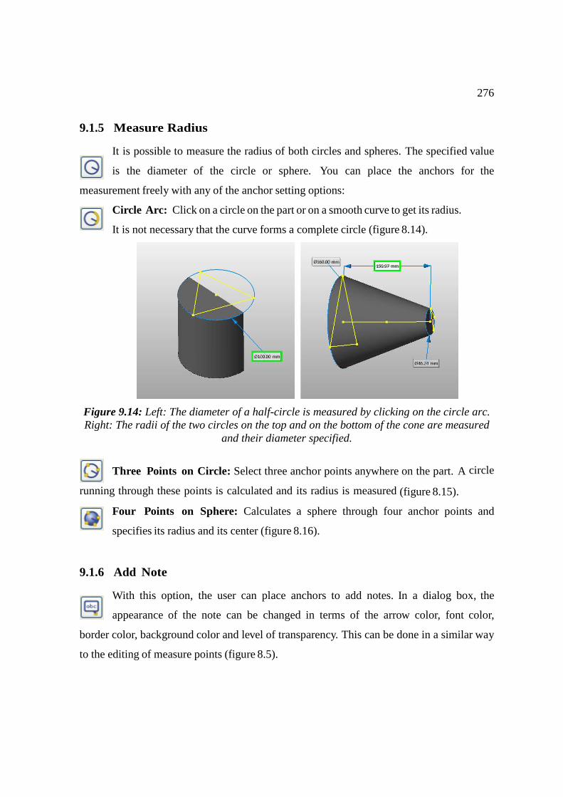
276
9.1.5 Measure Radius
It is possible to measure the radius of both circles and spheres. The specified value
is the diameter of the circle or sphere. You can place the anchors for the
measurement freely with any of the anchor setting options:
Circle Arc: Click on a circle on the part or on a smooth curve to get its radius.
It is not necessary that the curve forms a complete circle (figure 8.14).
Figure 9.14: Left: The diameter of a half-circle is measured by clicking on the circle arc. Right: The radii of the two circles on the top and on the bottom of the cone are measured
and their diameter specified.
Three Points on Circle: Select three anchor points anywhere on the part. A circle
running through these points is calculated and its radius is measured (figure 8.15).
Four Points on Sphere: Calculates a sphere through four anchor points and
specifies its radius and its center (figure 8.16).
9.1.6 Add Note
With this option, the user can place anchors to add notes. In a dialog box, the
appearance of the note can be changed in terms of the arrow color, font color,
border color, background color and level of transparency. This can be done in a similar way
to the editing of measure points (figure 8.5).
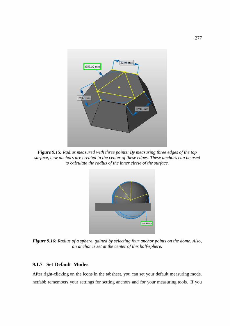
277
Figure 9.15: Radius measured with three points: By measuring three edges of the top surface, new anchors are created in the center of these edges. These anchors can be used
to calculate the radius of the inner circle of the surface.
Figure 9.16: Radius of a sphere, gained by selecting four anchor points on the dome. Also,
an anchor is set at the center of this half-sphere.
9.1.7 Set Default Modes
After right-clicking on the icons in the tabsheet, you can set your default measuring mode.
netfabb remembers your settings for setting anchors and for your measuring tools. If you
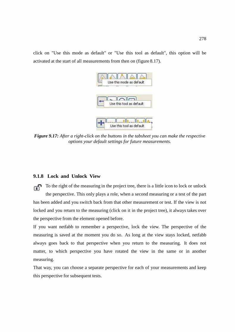
278
click on "Use this mode as default" or "Use this tool as default", this option will be
activated at the start of all measurements from then on (figure 8.17).
Figure 9.17: After a right-click on the buttons in the tabsheet you can make the respective options your default settings for future measurements.
9.1.8 Lock and Unlock View
To the right of the measuring in the project tree, there is a little icon to lock or unlock
the perspective. This only plays a role, when a second measuring or a test of the part
has been added and you switch back from that other measurement or test. If the view is not
locked and you return to the measuring (click on it in the project tree), it always takes over
the perspective from the element opened before.
If you want netfabb to remember a perspective, lock the view. The perspective of the
measuring is saved at the moment you do so. As long at the view stays locked, netfabb
always goes back to that perspective when you return to the measuring. It does not
matter, to which perspective you have rotated the view in the same or in another
measuring.
That way, you can choose a separate perspective for each of your measurements and keep
this perspective for subsequent tests.
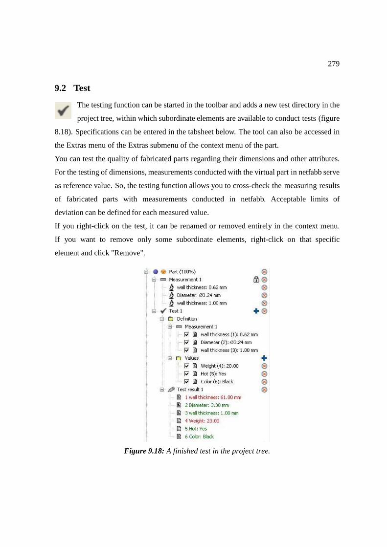
279
9.2 Test
The testing function can be started in the toolbar and adds a new test directory in the
project tree, within which subordinate elements are available to conduct tests (figure
8.18). Specifications can be entered in the tabsheet below. The tool can also be accessed in
the Extras menu of the Extras submenu of the context menu of the part.
You can test the quality of fabricated parts regarding their dimensions and other attributes.
For the testing of dimensions, measurements conducted with the virtual part in netfabb serve
as reference value. So, the testing function allows you to cross-check the measuring results
of fabricated parts with measurements conducted in netfabb. Acceptable limits of
deviation can be defined for each measured value.
If you right-click on the test, it can be renamed or removed entirely in the context menu.
If you want to remove only some subordinate elements, right-click on that specific
element and click "Remove".
Figure 9.18: A finished test in the project tree.
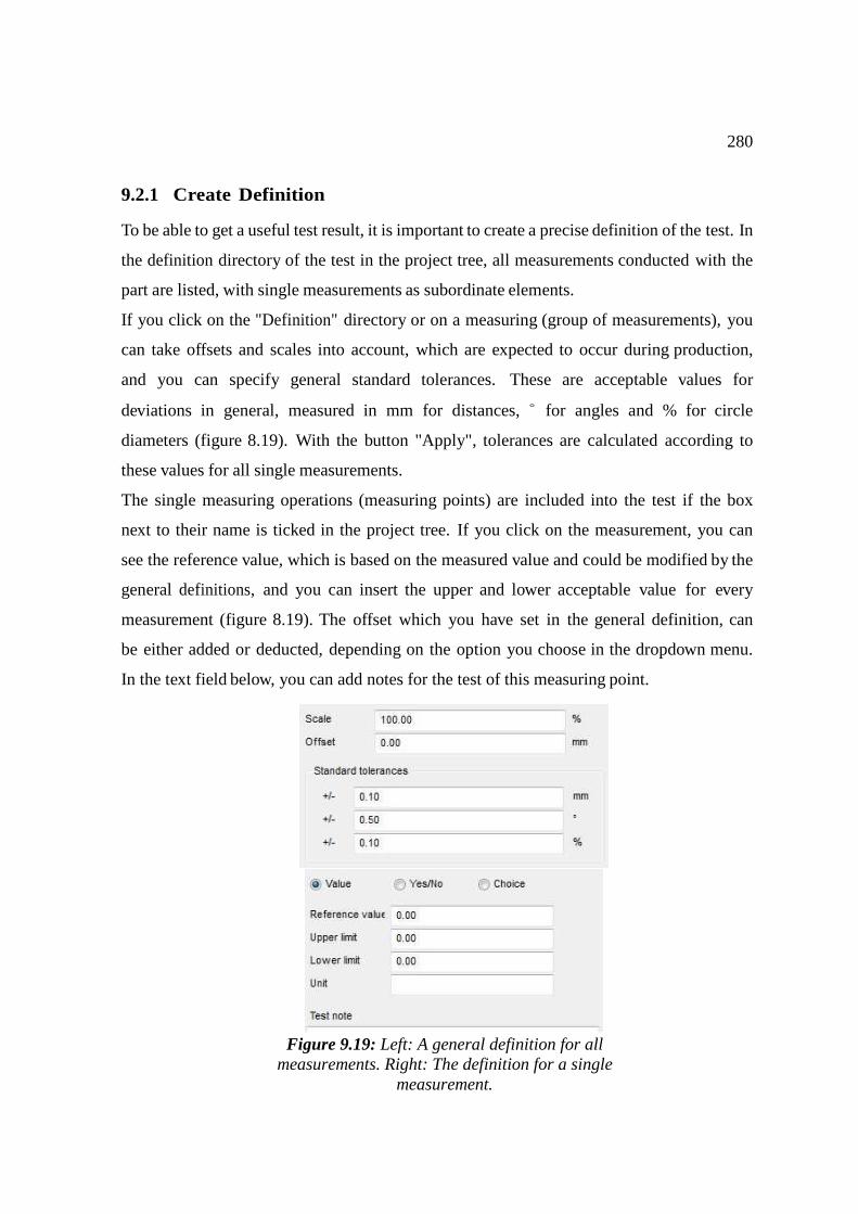
280
9.2.1 Create Definition
To be able to get a useful test result, it is important to create a precise definition of the test. In
the definition directory of the test in the project tree, all measurements conducted with the
part are listed, with single measurements as subordinate elements.
If you click on the "Definition" directory or on a measuring (group of measurements), you
can take offsets and scales into account, which are expected to occur during production,
and you can specify general standard tolerances. These are acceptable values for
deviations in general, measured in mm for distances, ◦ for angles and % for circle
diameters (figure 8.19). With the button "Apply", tolerances are calculated according to
these values for all single measurements.
The single measuring operations (measuring points) are included into the test if the box
next to their name is ticked in the project tree. If you click on the measurement, you can
see the reference value, which is based on the measured value and could be modified by the
general definitions, and you can insert the upper and lower acceptable value for every
measurement (figure 8.19). The offset which you have set in the general definition, can
be either added or deducted, depending on the option you choose in the dropdown menu.
In the text field below, you can add notes for the test of this measuring point.
Figure 9.19: Left: A general definition for all measurements. Right: The definition for a single
measurement.
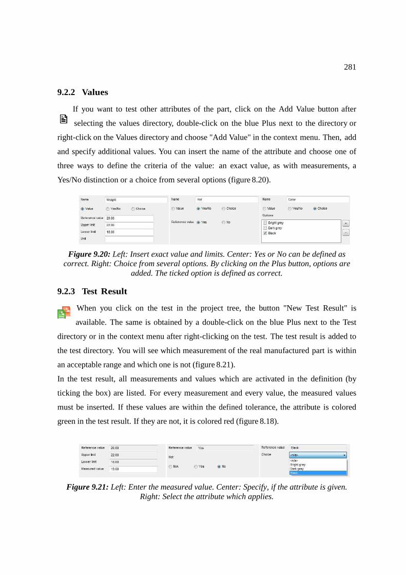
281
9.2.2 Values
If you want to test other attributes of the part, click on the Add Value button after
selecting the values directory, double-click on the blue Plus next to the directory or
right-click on the Values directory and choose "Add Value" in the context menu. Then, add
and specify additional values. You can insert the name of the attribute and choose one of
three ways to define the criteria of the value: an exact value, as with measurements, a
Yes/No distinction or a choice from several options (figure 8.20).
Figure 9.20: Left: Insert exact value and limits. Center: Yes or No can be defined as correct. Right: Choice from several options. By clicking on the Plus button, options are
added. The ticked option is defined as correct.
9.2.3 Test Result
When you click on the test in the project tree, the button "New Test Result" is
available. The same is obtained by a double-click on the blue Plus next to the Test
directory or in the context menu after right-clicking on the test. The test result is added to
the test directory. You will see which measurement of the real manufactured part is within
an acceptable range and which one is not (figure 8.21).
In the test result, all measurements and values which are activated in the definition (by
ticking the box) are listed. For every measurement and every value, the measured values
must be inserted. If these values are within the defined tolerance, the attribute is colored
green in the test result. If they are not, it is colored red (figure 8.18).
Figure 9.21: Left: Enter the measured value. Center: Specify, if the attribute is given. Right: Select the attribute which applies.
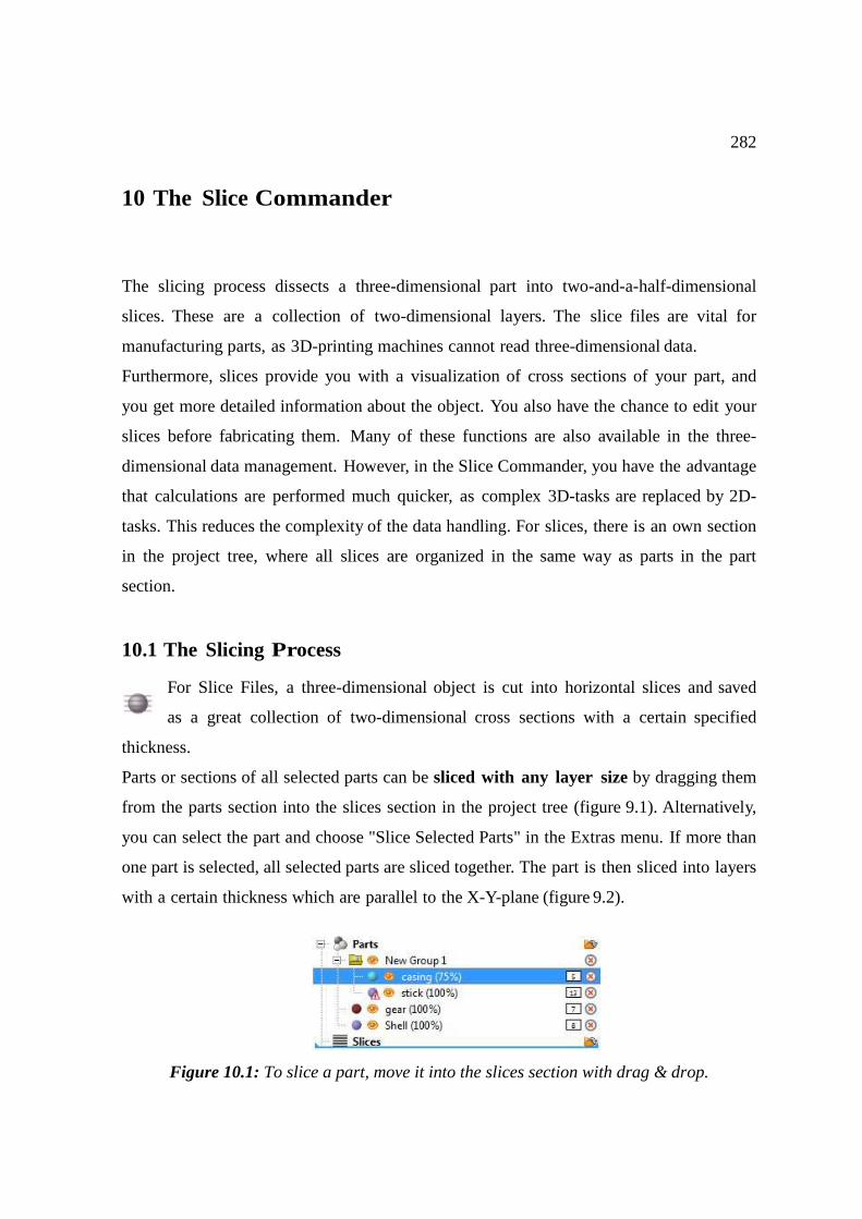
282
10 The Slice Commander
The slicing process dissects a three-dimensional part into two-and-a-half-dimensional
slices. These are a collection of two-dimensional layers. The slice files are vital for
manufacturing parts, as 3D-printing machines cannot read three-dimensional data.
Furthermore, slices provide you with a visualization of cross sections of your part, and
you get more detailed information about the object. You also have the chance to edit your
slices before fabricating them. Many of these functions are also available in the three-
dimensional data management. However, in the Slice Commander, you have the advantage
that calculations are performed much quicker, as complex 3D-tasks are replaced by 2D-
tasks. This reduces the complexity of the data handling. For slices, there is an own section
in the project tree, where all slices are organized in the same way as parts in the part
section.
10.1 The Slicing Process
For Slice Files, a three-dimensional object is cut into horizontal slices and saved
as a great collection of two-dimensional cross sections with a certain specified
thickness.
Parts or sections of all selected parts can be sliced with any layer size by dragging them
from the parts section into the slices section in the project tree (figure 9.1). Alternatively,
you can select the part and choose "Slice Selected Parts" in the Extras menu. If more than
one part is selected, all selected parts are sliced together. The part is then sliced into layers
with a certain thickness which are parallel to the X-Y-plane (figure 9.2).
Figure 10.1: To slice a part, move it into the slices section with drag & drop.
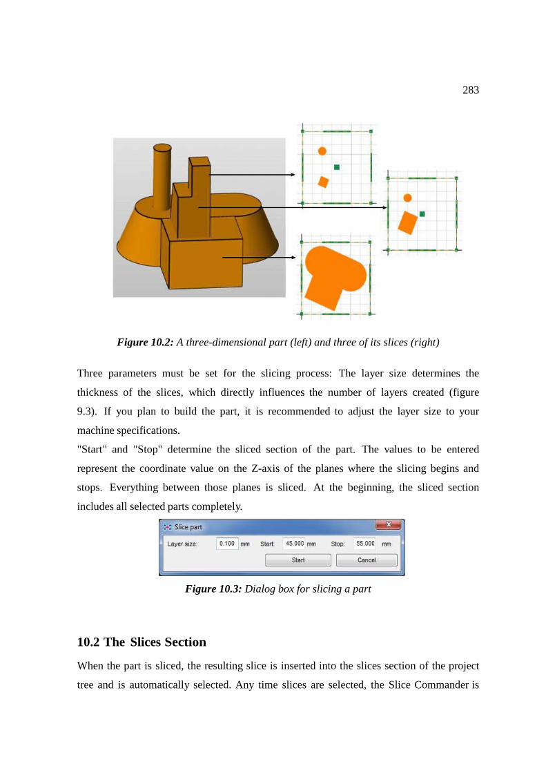
283
Figure 10.2: A three-dimensional part (left) and three of its slices (right)
Three parameters must be set for the slicing process: The layer size determines the
thickness of the slices, which directly influences the number of layers created (figure
9.3). If you plan to build the part, it is recommended to adjust the layer size to your
machine specifications.
"Start" and "Stop" determine the sliced section of the part. The values to be entered
represent the coordinate value on the Z-axis of the planes where the slicing begins and
stops. Everything between those planes is sliced. At the beginning, the sliced section
includes all selected parts completely.
Figure 10.3: Dialog box for slicing a part
10.2 The Slices Section
When the part is sliced, the resulting slice is inserted into the slices section of the project
tree and is automatically selected. Any time slices are selected, the Slice Commander is

284
activated. Changing slices in the Slice Commander does not have any influence on original
three-dimensional parts in your project.
The viewing screen is replaced by a slices screen, where slices are displayed layer-by-
layer. Slice viewing and handling options are available in the tabsheet, in the context menu
of the screen (figure 9.4) and in a Slices menu, which is added to the menu bar.
Previously saved slice files with various file formats can alternatively be opened and
inserted into the project with the File Preview Browser or with the option "Open Slice File"
in the context menu.
Just as parts in the normal mode, slices can also be assigned to groups. These are
created in the context menu and appear as a directory in the "Slices" section of the
project tree. Slices can be moved into and out of groups by drag & drop, in the same way
as parts (chapter 5.7)
If you want to remove slices, you can either double click on the red X to the right
of the slice in the project tree, choose "Remove" in the context menu or simply press
Delete when the slice is selected. If you choose "Remove all", all slices will be removed
and the Slice Commander will be emptied. For further information about the Export
functions in the Slice commander, take a look at chapter 9.7.
Slices can be duplicated in the context menu. That way, an exact copy of the slice
file is inserted to the right of the original.
10.3 Active Slice File
In the tabsheet, information can be viewed on the selected slice file. It contains the name
of the current slice, the size of the whole part, its area, contour length and hatches
length. Min. Z and Max. Z give you the exact position along the axis.
The scroll bar on the left regulates the display of layers from top to bottom. You can
also scroll through slice layers with your mouse wheel, if you hold the Alt-button. If
a slice animation is started, the Slice Commander automatically browses through the
slices at a chosen speed (Layers per Second).
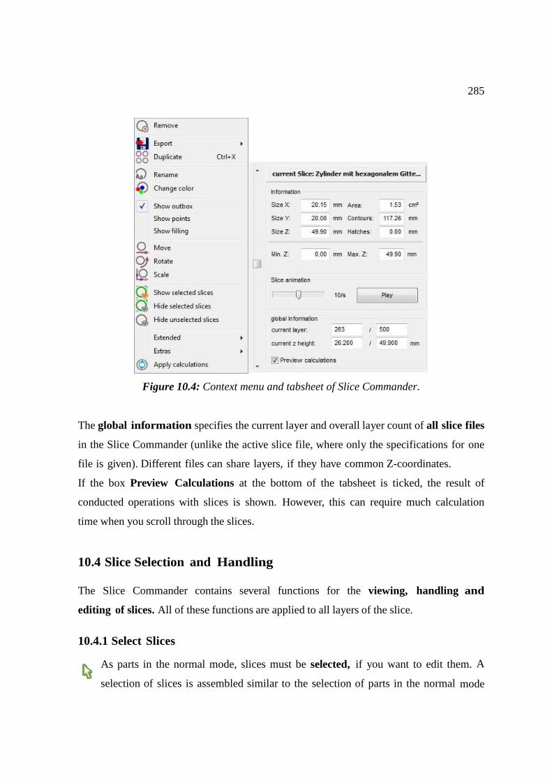
285
Figure 10.4: Context menu and tabsheet of Slice Commander.
The global information specifies the current layer and overall layer count of all slice files
in the Slice Commander (unlike the active slice file, where only the specifications for one
file is given). Different files can share layers, if they have common Z-coordinates.
If the box Preview Calculations at the bottom of the tabsheet is ticked, the result of
conducted operations with slices is shown. However, this can require much calculation
time when you scroll through the slices.
10.4 Slice Selection and Handling
The Slice Commander contains several functions for the viewing, handling and
editing of slices. All of these functions are applied to all layers of the slice.
10.4.1 Select Slices
As parts in the normal mode, slices must be selected, if you want to edit them. A
selection of slices is assembled similar to the selection of parts in the normal mode
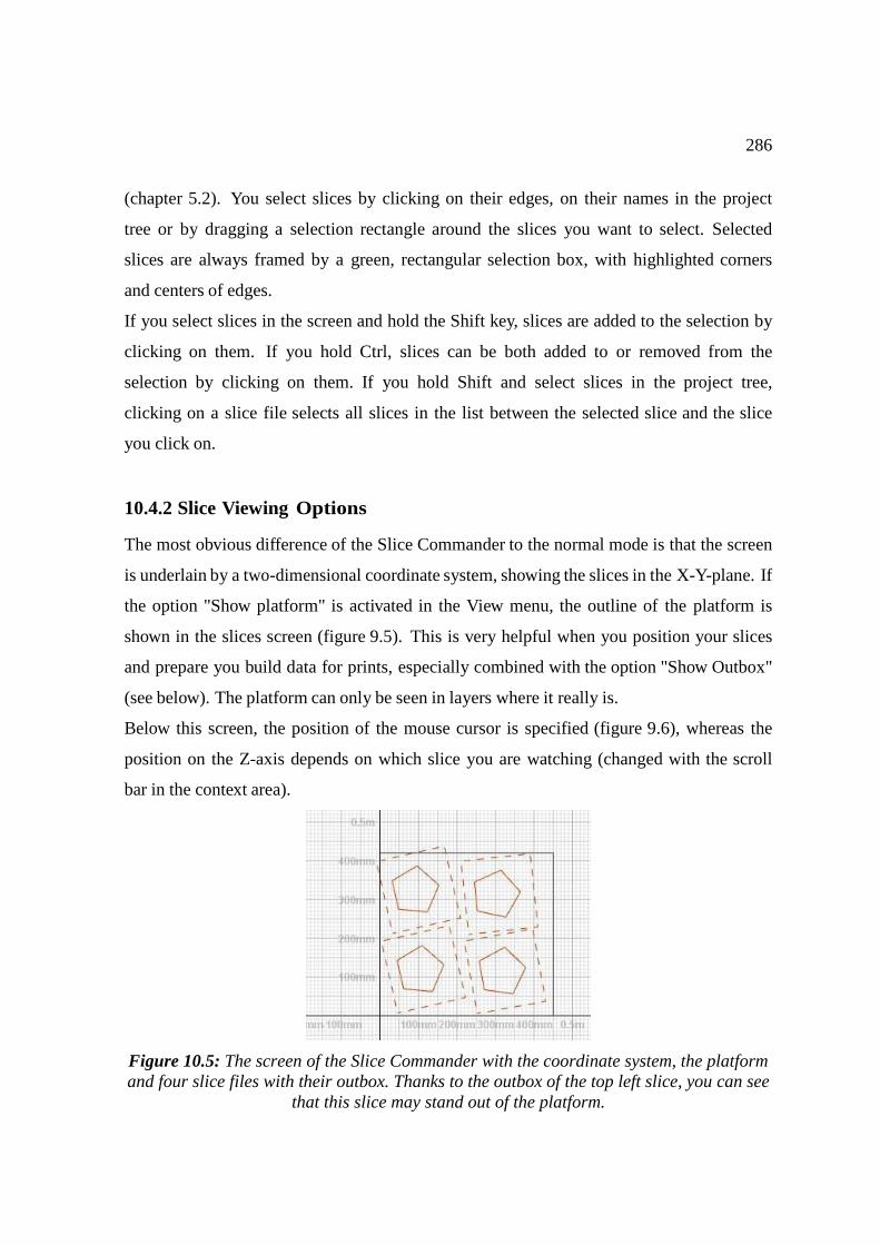
286
(chapter 5.2). You select slices by clicking on their edges, on their names in the project
tree or by dragging a selection rectangle around the slices you want to select. Selected
slices are always framed by a green, rectangular selection box, with highlighted corners
and centers of edges.
If you select slices in the screen and hold the Shift key, slices are added to the selection by
clicking on them. If you hold Ctrl, slices can be both added to or removed from the
selection by clicking on them. If you hold Shift and select slices in the project tree,
clicking on a slice file selects all slices in the list between the selected slice and the slice
you click on.
10.4.2 Slice Viewing Options
The most obvious difference of the Slice Commander to the normal mode is that the screen
is underlain by a two-dimensional coordinate system, showing the slices in the X-Y-plane. If
the option "Show platform" is activated in the View menu, the outline of the platform is
shown in the slices screen (figure 9.5). This is very helpful when you position your slices
and prepare you build data for prints, especially combined with the option "Show Outbox"
(see below). The platform can only be seen in layers where it really is.
Below this screen, the position of the mouse cursor is specified (figure 9.6), whereas the
position on the Z-axis depends on which slice you are watching (changed with the scroll
bar in the context area).
Figure 10.5: The screen of the Slice Commander with the coordinate system, the platform and four slice files with their outbox. Thanks to the outbox of the top left slice, you can see
that this slice may stand out of the platform.
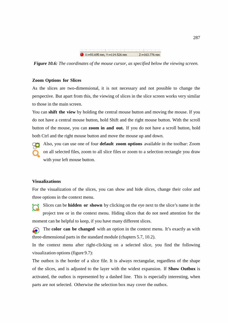
287
Figure 10.6: The coordinates of the mouse cursor, as specified below the viewing screen.
Zoom Options for Slices
As the slices are two-dimensional, it is not necessary and not possible to change the
perspective. But apart from this, the viewing of slices in the slice screen works very similar
to those in the main screen.
You can shift the view by holding the central mouse button and moving the mouse. If you
do not have a central mouse button, hold Shift and the right mouse button. With the scroll
button of the mouse, you can zoom in and out. If you do not have a scroll button, hold
both Ctrl and the right mouse button and move the mouse up and down.
Also, you can use one of four default zoom options available in the toolbar: Zoom
on all selected files, zoom to all slice files or zoom to a selection rectangle you draw
with your left mouse button.
Visualizations
For the visualization of the slices, you can show and hide slices, change their color and
three options in the context menu.
Slices can be hidden or shown by clicking on the eye next to the slice’s name in the
project tree or in the context menu. Hiding slices that do not need attention for the
moment can be helpful to keep, if you have many different slices.
The color can be changed with an option in the context menu. It’s exactly as with
three-dimensional parts in the standard module (chapters 5.7, 10.2).
In the context menu after right-clicking on a selected slice, you find the following
visualization options (figure 9.7):
The outbox is the border of a slice file. It is always rectangular, regardless of the shape
of the slices, and is adjusted to the layer with the widest expansion. If Show Outbox is
activated, the outbox is represented by a dashed line. This is especially interesting, when
parts are not selected. Otherwise the selection box may cover the outbox.
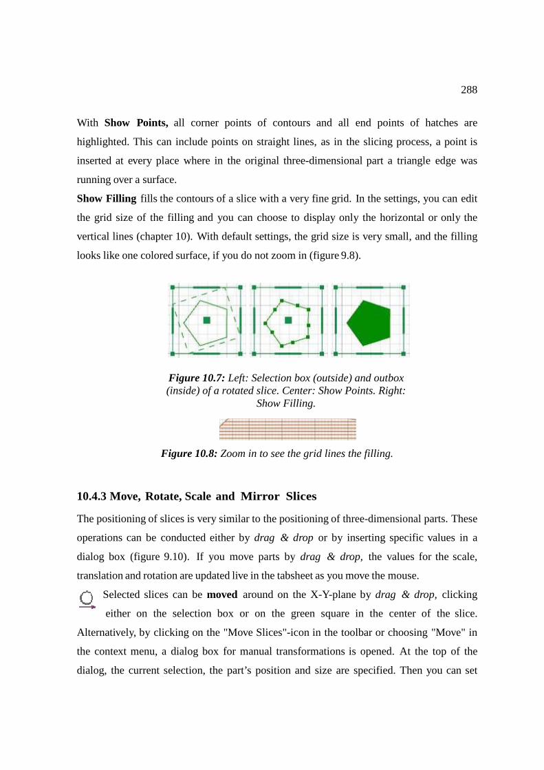
288
With Show Points, all corner points of contours and all end points of hatches are
highlighted. This can include points on straight lines, as in the slicing process, a point is
inserted at every place where in the original three-dimensional part a triangle edge was
running over a surface.
Show Filling fills the contours of a slice with a very fine grid. In the settings, you can edit
the grid size of the filling and you can choose to display only the horizontal or only the
vertical lines (chapter 10). With default settings, the grid size is very small, and the filling
looks like one colored surface, if you do not zoom in (figure 9.8).
Figure 10.8: Zoom in to see the grid lines the filling.
10.4.3 Move, Rotate, Scale and Mirror Slices
The positioning of slices is very similar to the positioning of three-dimensional parts. These
operations can be conducted either by drag & drop or by inserting specific values in a
dialog box (figure 9.10). If you move parts by drag & drop, the values for the scale,
translation and rotation are updated live in the tabsheet as you move the mouse.
Selected slices can be moved around on the X-Y-plane by drag & drop, clicking
either on the selection box or on the green square in the center of the slice.
Alternatively, by clicking on the "Move Slices"-icon in the toolbar or choosing "Move" in
the context menu, a dialog box for manual transformations is opened. At the top of the
dialog, the current selection, the part’s position and size are specified. Then you can set
Figure 10.7: Left: Selection box (outside) and outbox (inside) of a rotated slice. Center: Show Points. Right:
Show Filling.
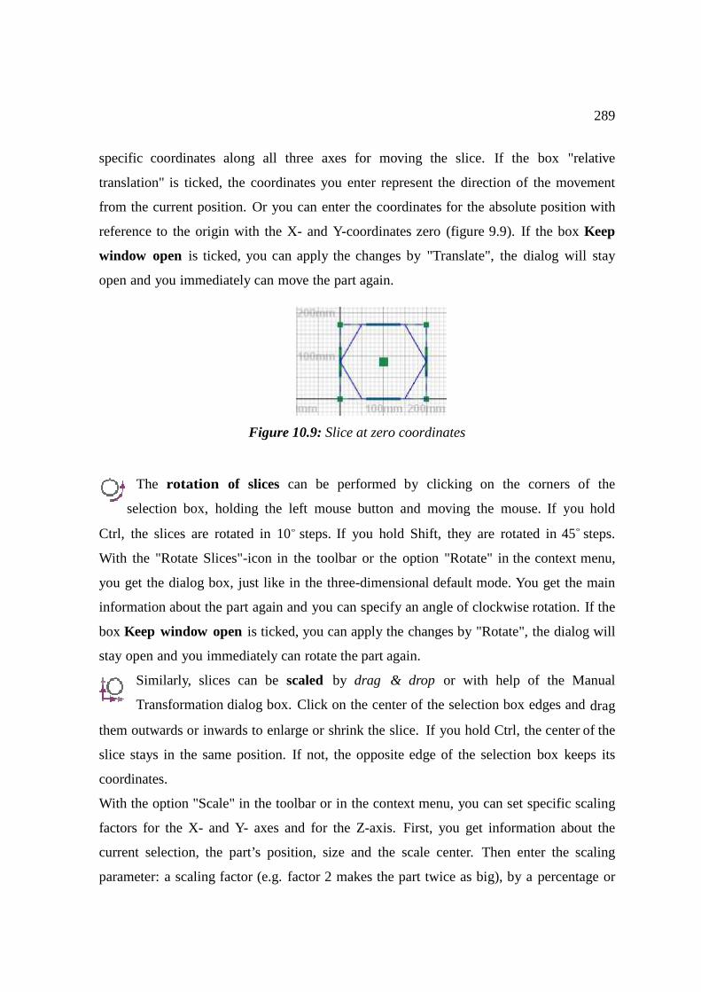
289
specific coordinates along all three axes for moving the slice. If the box "relative
translation" is ticked, the coordinates you enter represent the direction of the movement
from the current position. Or you can enter the coordinates for the absolute position with
reference to the origin with the X- and Y-coordinates zero (figure 9.9). If the box Keep
window open is ticked, you can apply the changes by "Translate", the dialog will stay
open and you immediately can move the part again.
Figure 10.9: Slice at zero coordinates
The rotation of slices can be performed by clicking on the corners of the
selection box, holding the left mouse button and moving the mouse. If you hold
Ctrl, the slices are rotated in 10◦ steps. If you hold Shift, they are rotated in 45◦ steps.
With the "Rotate Slices"-icon in the toolbar or the option "Rotate" in the context menu,
you get the dialog box, just like in the three-dimensional default mode. You get the main
information about the part again and you can specify an angle of clockwise rotation. If the
box Keep window open is ticked, you can apply the changes by "Rotate", the dialog will
stay open and you immediately can rotate the part again.
Similarly, slices can be scaled by drag & drop or with help of the Manual
Transformation dialog box. Click on the center of the selection box edges and drag
them outwards or inwards to enlarge or shrink the slice. If you hold Ctrl, the center of the
slice stays in the same position. If not, the opposite edge of the selection box keeps its
coordinates.
With the option "Scale" in the toolbar or in the context menu, you can set specific scaling
factors for the X- and Y- axes and for the Z-axis. First, you get information about the
current selection, the part’s position, size and the scale center. Then enter the scaling
parameter: a scaling factor (e.g. factor 2 makes the part twice as big), by a percentage or
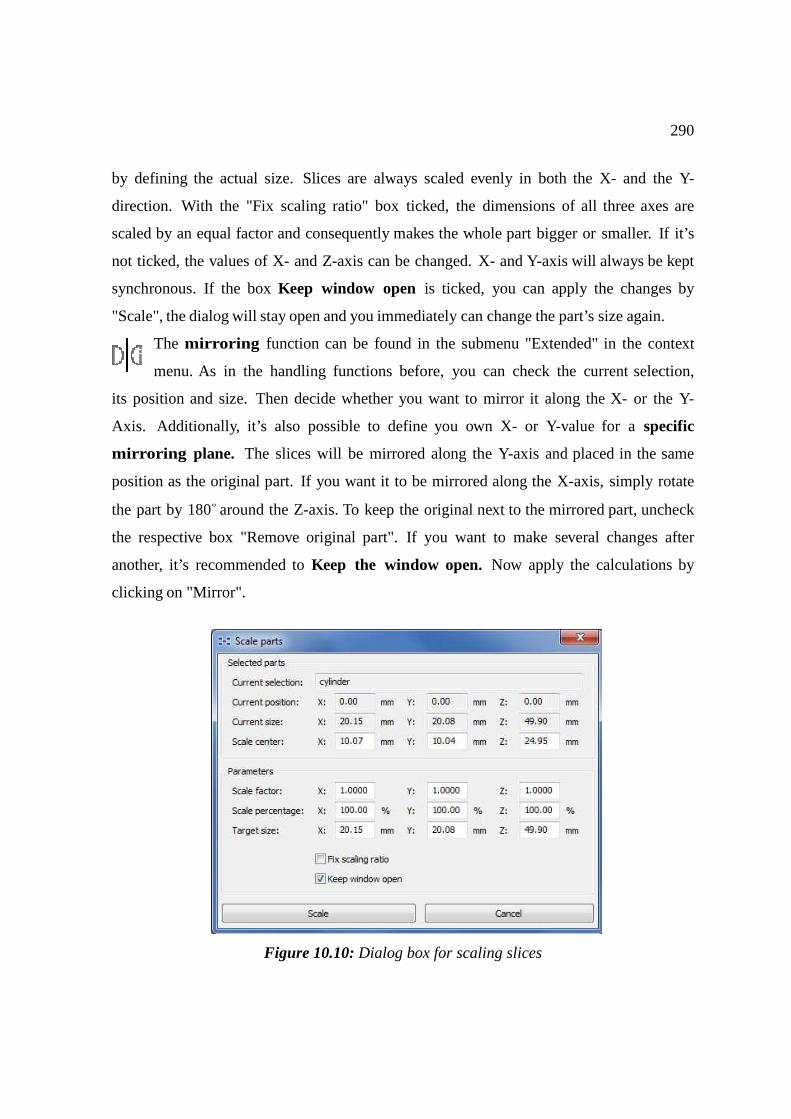
290
by defining the actual size. Slices are always scaled evenly in both the X- and the Y-
direction. With the "Fix scaling ratio" box ticked, the dimensions of all three axes are
scaled by an equal factor and consequently makes the whole part bigger or smaller. If it’s
not ticked, the values of X- and Z-axis can be changed. X- and Y-axis will always be kept
synchronous. If the box Keep window open is ticked, you can apply the changes by
"Scale", the dialog will stay open and you immediately can change the part’s size again.
The mirroring function can be found in the submenu "Extended" in the context
menu. As in the handling functions before, you can check the current selection,
its position and size. Then decide whether you want to mirror it along the X- or the Y-
Axis. Additionally, it’s also possible to define you own X- or Y-value for a specific
mirroring plane. The slices will be mirrored along the Y-axis and placed in the same
position as the original part. If you want it to be mirrored along the X-axis, simply rotate
the part by 180◦ around the Z-axis. To keep the original next to the mirrored part, uncheck
the respective box "Remove original part". If you want to make several changes after
another, it’s recommended to Keep the window open. Now apply the calculations by
clicking on "Mirror".
Figure 10.10: Dialog box for scaling slices
291
10.4.4 Merging and Grouping
When two parts or more are selected, the slices can be unified to one single part. The
original shapes will remain and can be separated again later.
In the submenu "Extended" in the context menu, there’s the option Merge
Slices: The slices will become one slice file which includes all contours of the original.
Overlapping contours will remain.
With Clear grouping you can reverse this unification. And very importantly,
editing operations you conduct with slices, such as merging slices, can also be undone
by this function. Thereafter, the slice resulting from the operation is removed and a new
group is created which will contain the original slices.
10.5 Edit Slices
Many of these functions are also available in the three-dimensional data management.
However, in the Slice Commander, you have the advantage that calculations are performed
much quicker, as complex 3D-tasks are replaced by 2D-tasks. This reduces the
complexity of the data handling.
The result of editing slices can be seen when the box Preview Calculations at the bottom
of the tabsheet is ticked. However, this can require much calculation time when you scroll
through the slices. If "Preview Calculations" is not ticked, the original slices are displayed
until the calculations are applied.
The same calculations can be ultimately implemented by choosing Apply
Calculations in the context menu. Please note that calculations are applied
automatically when you export the slice.
As long as the calculations have not yet been applied, editing operations with slices
can be undone by selecting Clear grouping in the context menu. The slice
resulting from the operation is removed and a new group is created which will contain the
original slices.

292
10.5.1 Boolean Operations & Removing Self-Intersections
If one part is selected that contains self-intersections, you can also remove them in the
slices. Or if two or more parts are selected, you can perform Boolean operations. Find both
functions in the context menu in the submenu Extended. If one part is selected, you’ll find
the "Remove self-intersections" button, if more parts are selected, the "Boolean Operation"
button will be displayed instead.
The Boolean Operation allows you to merge overlapping slices, create an
intersection, or subtract one slice from the other (figure 9.11). A dialog box appears in
which the selected slice files can be assigned to the two fields "Add" and "Subtract". At the
beginning, all slices are in "Add". If you click on a slice and then click on the arrow
pointing to the other field, the file is moved there. If you click on the X, the selected file is
removed.
To unify slices, all slices have to be in the left field "Add". Execute the unification with
the button "Boolean" (figure 9.12). For an intersection of selected slices, choose "Create
Intersection" in the context menu instead of "Boolean Operation". The resulting slice
includes only the overlap ping sections of all selected slices (figure 9.12).
Figure 10.11: Top left: Two overlapping slices. Top right: A unification of those slices. Bottom left: The intersection of the slices. Bottom right: One slice is subtracted.
Figure 10.12: Left: Two overlapping slices. Center: Unify. Right: Intersection.
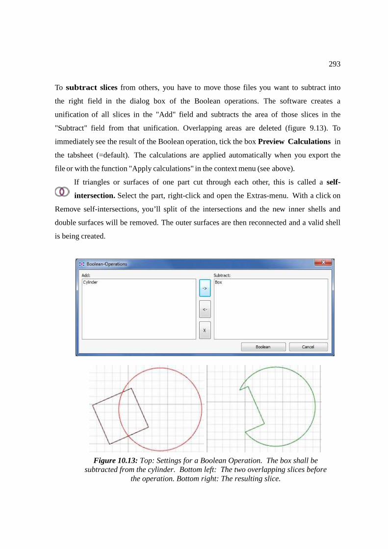
293
To subtract slices from others, you have to move those files you want to subtract into
the right field in the dialog box of the Boolean operations. The software creates a
unification of all slices in the "Add" field and subtracts the area of those slices in the
"Subtract" field from that unification. Overlapping areas are deleted (figure 9.13). To
immediately see the result of the Boolean operation, tick the box Preview Calculations in
the tabsheet (=default). The calculations are applied automatically when you export the
file or with the function "Apply calculations" in the context menu (see above).
If triangles or surfaces of one part cut through each other, this is called a self-
intersection. Select the part, right-click and open the Extras-menu. With a click on
Remove self-intersections, you’ll split of the intersections and the new inner shells and
double surfaces will be removed. The outer surfaces are then reconnected and a valid shell
is being created.
Figure 10.13: Top: Settings for a Boolean Operation. The box shall be subtracted from the cylinder. Bottom left: The two overlapping slices before
the operation. Bottom right: The resulting slice.
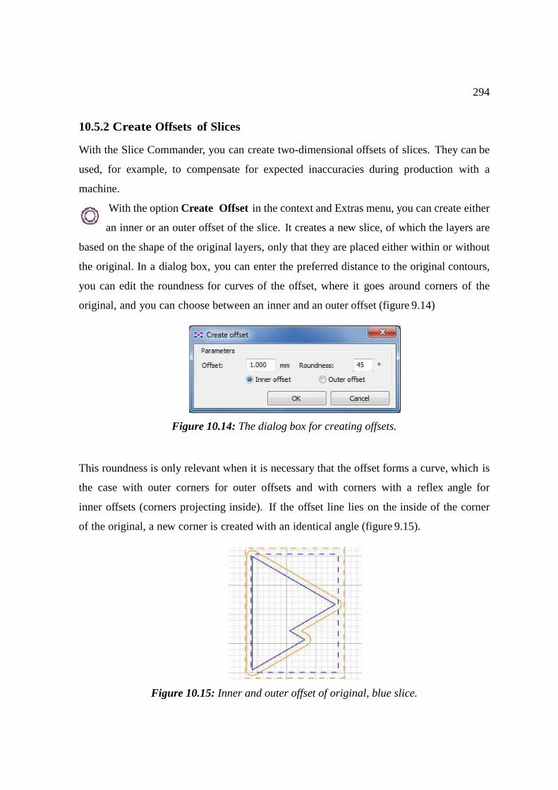
294
10.5.2 Create Offsets of Slices
With the Slice Commander, you can create two-dimensional offsets of slices. They can be
used, for example, to compensate for expected inaccuracies during production with a
machine.
With the option Create Offset in the context and Extras menu, you can create either
an inner or an outer offset of the slice. It creates a new slice, of which the layers are
based on the shape of the original layers, only that they are placed either within or without
the original. In a dialog box, you can enter the preferred distance to the original contours,
you can edit the roundness for curves of the offset, where it goes around corners of the
original, and you can choose between an inner and an outer offset (figure 9.14)
Figure 10.14: The dialog box for creating offsets.
This roundness is only relevant when it is necessary that the offset forms a curve, which is
the case with outer corners for outer offsets and with corners with a reflex angle for
inner offsets (corners projecting inside). If the offset line lies on the inside of the corner
of the original, a new corner is created with an identical angle (figure 9.15).
Figure 10.15: Inner and outer offset of original, blue slice.
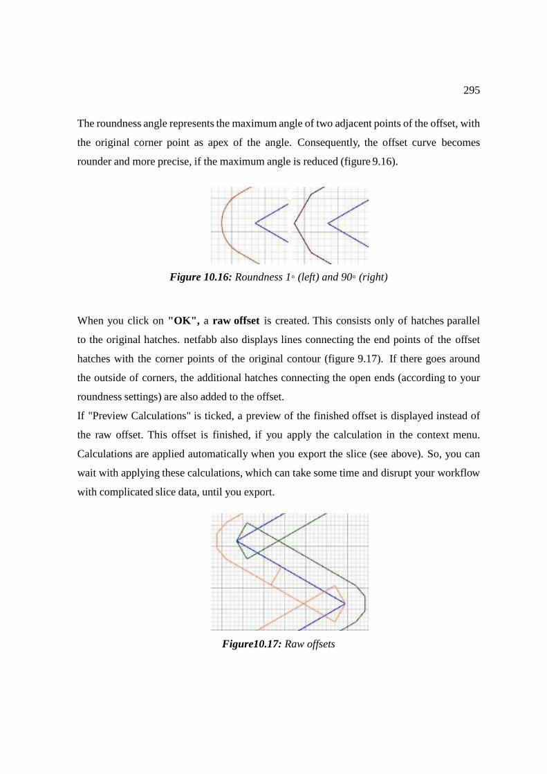
295
The roundness angle represents the maximum angle of two adjacent points of the offset, with
the original corner point as apex of the angle. Consequently, the offset curve becomes
rounder and more precise, if the maximum angle is reduced (figure 9.16).
Figure 10.16: Roundness 1◦ (left) and 90◦ (right)
When you click on "OK", a raw offset is created. This consists only of hatches parallel
to the original hatches. netfabb also displays lines connecting the end points of the offset
hatches with the corner points of the original contour (figure 9.17). If there goes around
the outside of corners, the additional hatches connecting the open ends (according to your
roundness settings) are also added to the offset.
If "Preview Calculations" is ticked, a preview of the finished offset is displayed instead of
the raw offset. This offset is finished, if you apply the calculation in the context menu.
Calculations are applied automatically when you export the slice (see above). So, you can
wait with applying these calculations, which can take some time and disrupt your workflow
with complicated slice data, until you export.
Figure10.17: Raw offsets
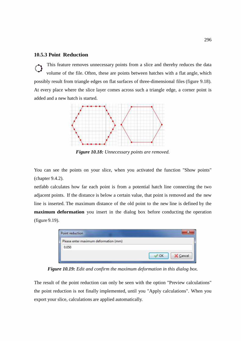
296
10.5.3 Point Reduction
This feature removes unnecessary points from a slice and thereby reduces the data
volume of the file. Often, these are points between hatches with a flat angle, which
possibly result from triangle edges on flat surfaces of three-dimensional files (figure 9.18).
At every place where the slice layer comes across such a triangle edge, a corner point is
added and a new hatch is started.
Figure 10.18: Unnecessary points are removed.
You can see the points on your slice, when you activated the function "Show points"
(chapter 9.4.2).
netfabb calculates how far each point is from a potential hatch line connecting the two
adjacent points. If the distance is below a certain value, that point is removed and the new
line is inserted. The maximum distance of the old point to the new line is defined by the
maximum deformation you insert in the dialog box before conducting the operation
(figure 9.19).
Figure 10.19: Edit and confirm the maximum deformation in this dialog box.
The result of the point reduction can only be seen with the option "Preview calculations"
the point reduction is not finally implemented, until you "Apply calculations". When you
export your slice, calculations are applied automatically.
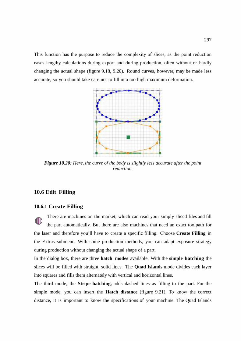
297
This function has the purpose to reduce the complexity of slices, as the point reduction
eases lengthy calculations during export and during production, often without or hardly
changing the actual shape (figure 9.18, 9.20). Round curves, however, may be made less
accurate, so you should take care not to fill in a too high maximum deformation.
Figure 10.20: Here, the curve of the body is slightly less accurate after the point reduction.
10.6 Edit Filling
10.6.1 Create Filling
There are machines on the market, which can read your simply sliced files and fill
the part automatically. But there are also machines that need an exact toolpath for
the laser and therefore you’ll have to create a specific filling. Choose Create Filling in
the Extras submenu. With some production methods, you can adapt exposure strategy
during production without changing the actual shape of a part.
In the dialog box, there are three hatch modes available. With the simple hatching the
slices will be filled with straight, solid lines. The Quad Islands mode divides each layer
into squares and fills them alternately with vertical and horizontal lines.
The third mode, the Stripe hatching, adds dashed lines as filling to the part. For the
simple mode, you can insert the Hatch distance (figure 9.21). To know the correct
distance, it is important to know the specifications of your machine. The Quad Islands
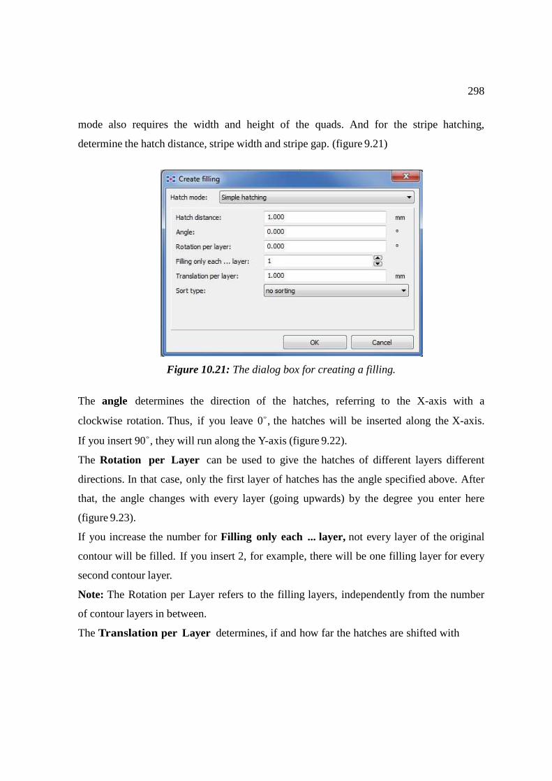
298
mode also requires the width and height of the quads. And for the stripe hatching,
determine the hatch distance, stripe width and stripe gap. (figure 9.21)
Figure 10.21: The dialog box for creating a filling.
The angle determines the direction of the hatches, referring to the X-axis with a
clockwise rotation. Thus, if you leave 0◦, the hatches will be inserted along the X-axis.
If you insert 90◦, they will run along the Y-axis (figure 9.22).
The Rotation per Layer can be used to give the hatches of different layers different
directions. In that case, only the first layer of hatches has the angle specified above. After
that, the angle changes with every layer (going upwards) by the degree you enter here
(figure 9.23).
If you increase the number for Filling only each ... layer, not every layer of the original
contour will be filled. If you insert 2, for example, there will be one filling layer for every
second contour layer.
Note: The Rotation per Layer refers to the filling layers, independently from the number
of contour layers in between.
The Translation per Layer determines, if and how far the hatches are shifted with
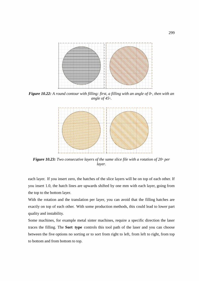
299
Figure 10.22: A round contour with filling: first, a filling with an angle of 0◦, then with an angle of 45◦.
Figure 10.23: Two consecutive layers of the same slice file with a rotation of 20◦ per
layer.
each layer. If you insert zero, the hatches of the slice layers will be on top of each other. If
you insert 1.0, the hatch lines are upwards shifted by one mm with each layer, going from
the top to the bottom layer.
With the rotation and the translation per layer, you can avoid that the filling hatches are
exactly on top of each other. With some production methods, this could lead to lower part
quality and instability.
Some machines, for example metal sinter machines, require a specific direction the laser
traces the filling. The Sort type controls this tool path of the laser and you can choose
between the five options no sorting or to sort from right to left, from left to right, from top
to bottom and from bottom to top.
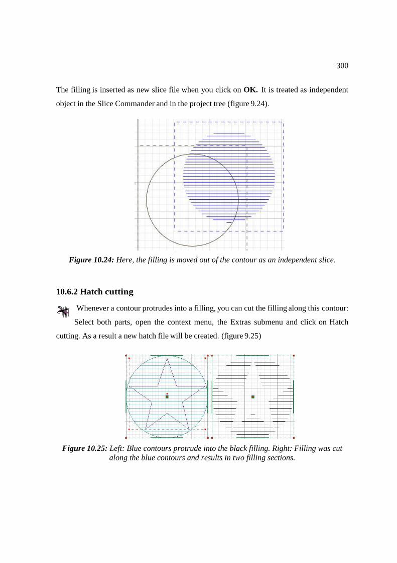
300
The filling is inserted as new slice file when you click on OK. It is treated as independent
object in the Slice Commander and in the project tree (figure 9.24).
Figure 10.24: Here, the filling is moved out of the contour as an independent slice.
10.6.2 Hatch cutting
Whenever a contour protrudes into a filling, you can cut the filling along this contour:
Select both parts, open the context menu, the Extras submenu and click on Hatch
cutting. As a result a new hatch file will be created. (figure 9.25)
Figure 10.25: Left: Blue contours protrude into the black filling. Right: Filling was cut along the blue contours and results in two filling sections.
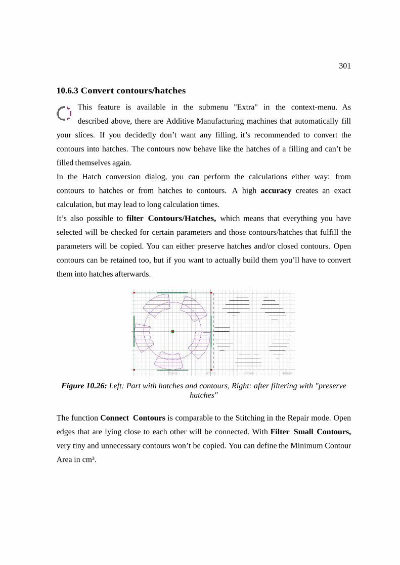
301
10.6.3 Convert contours/hatches
This feature is available in the submenu "Extra" in the context-menu. As
described above, there are Additive Manufacturing machines that automatically fill
your slices. If you decidedly don’t want any filling, it’s recommended to convert the
contours into hatches. The contours now behave like the hatches of a filling and can’t be
filled themselves again.
In the Hatch conversion dialog, you can perform the calculations either way: from
contours to hatches or from hatches to contours. A high accuracy creates an exact
calculation, but may lead to long calculation times.
It’s also possible to filter Contours/Hatches, which means that everything you have
selected will be checked for certain parameters and those contours/hatches that fulfill the
parameters will be copied. You can either preserve hatches and/or closed contours. Open
contours can be retained too, but if you want to actually build them you’ll have to convert
them into hatches afterwards.
Figure 10.26: Left: Part with hatches and contours, Right: after filtering with "preserve hatches"
The function Connect Contours is comparable to the Stitching in the Repair mode. Open
edges that are lying close to each other will be connected. With Filter Small Contours,
very tiny and unnecessary contours won’t be copied. You can define the Minimum Contour
Area in cm³.
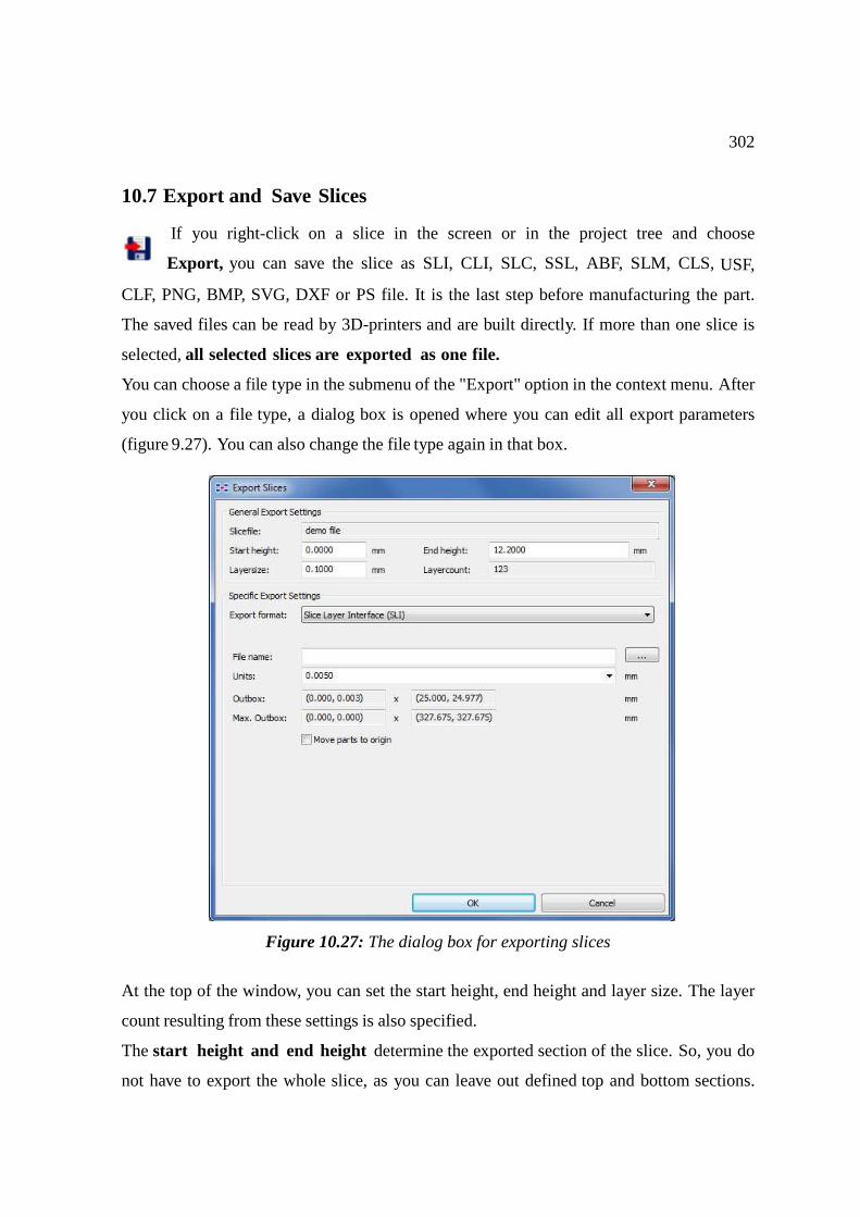
302
10.7 Export and Save Slices
If you right-click on a slice in the screen or in the project tree and choose
Export, you can save the slice as SLI, CLI, SLC, SSL, ABF, SLM, CLS, USF,
CLF, PNG, BMP, SVG, DXF or PS file. It is the last step before manufacturing the part.
The saved files can be read by 3D-printers and are built directly. If more than one slice is
selected, all selected slices are exported as one file.
You can choose a file type in the submenu of the "Export" option in the context menu. After
you click on a file type, a dialog box is opened where you can edit all export parameters
(figure 9.27). You can also change the file type again in that box.
Figure 10.27: The dialog box for exporting slices
At the top of the window, you can set the start height, end height and layer size. The layer
count resulting from these settings is also specified.
The start height and end height determine the exported section of the slice. So, you do
not have to export the whole slice, as you can leave out defined top and bottom sections.
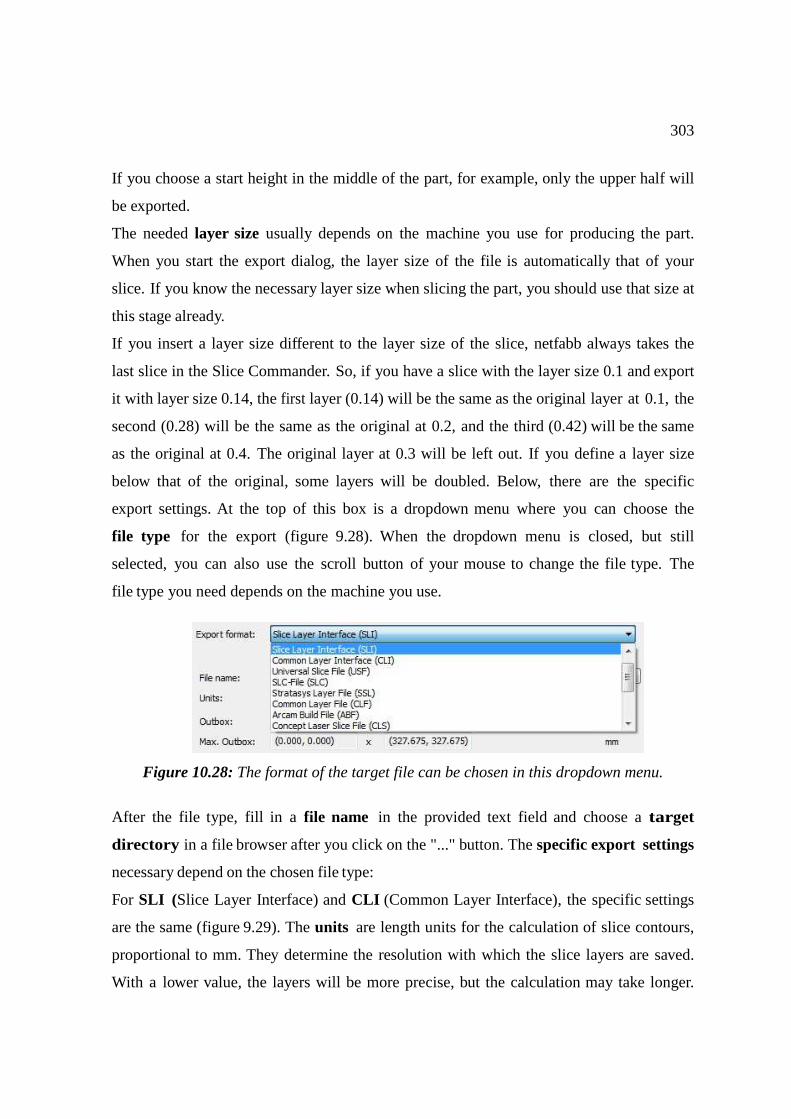
303
If you choose a start height in the middle of the part, for example, only the upper half will
be exported.
The needed layer size usually depends on the machine you use for producing the part.
When you start the export dialog, the layer size of the file is automatically that of your
slice. If you know the necessary layer size when slicing the part, you should use that size at
this stage already.
If you insert a layer size different to the layer size of the slice, netfabb always takes the
last slice in the Slice Commander. So, if you have a slice with the layer size 0.1 and export
it with layer size 0.14, the first layer (0.14) will be the same as the original layer at 0.1, the
second (0.28) will be the same as the original at 0.2, and the third (0.42) will be the same
as the original at 0.4. The original layer at 0.3 will be left out. If you define a layer size
below that of the original, some layers will be doubled. Below, there are the specific
export settings. At the top of this box is a dropdown menu where you can choose the
file type for the export (figure 9.28). When the dropdown menu is closed, but still
selected, you can also use the scroll button of your mouse to change the file type. The
file type you need depends on the machine you use.
Figure 10.28: The format of the target file can be chosen in this dropdown menu.
After the file type, fill in a file name in the provided text field and choose a target
directory in a file browser after you click on the "..." button. The specific export settings
necessary depend on the chosen file type:
For SLI (Slice Layer Interface) and CLI (Common Layer Interface), the specific settings
are the same (figure 9.29). The units are length units for the calculation of slice contours,
proportional to mm. They determine the resolution with which the slice layers are saved.
With a lower value, the layers will be more precise, but the calculation may take longer.
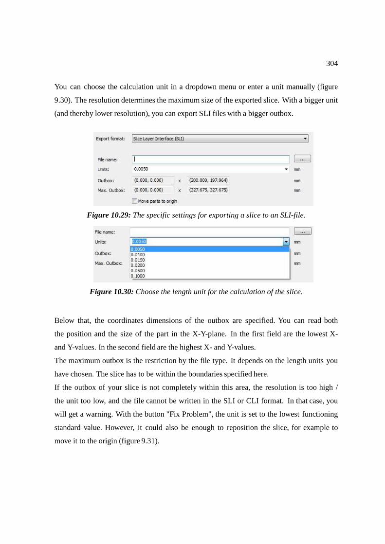
304
You can choose the calculation unit in a dropdown menu or enter a unit manually (figure
9.30). The resolution determines the maximum size of the exported slice. With a bigger unit
(and thereby lower resolution), you can export SLI files with a bigger outbox.
Figure 10.29: The specific settings for exporting a slice to an SLI-file.
Figure 10.30: Choose the length unit for the calculation of the slice.
Below that, the coordinates dimensions of the outbox are specified. You can read both
the position and the size of the part in the X-Y-plane. In the first field are the lowest X-
and Y-values. In the second field are the highest X- and Y-values.
The maximum outbox is the restriction by the file type. It depends on the length units you
have chosen. The slice has to be within the boundaries specified here.
If the outbox of your slice is not completely within this area, the resolution is too high /
the unit too low, and the file cannot be written in the SLI or CLI format. In that case, you
will get a warning. With the button "Fix Problem", the unit is set to the lowest functioning
standard value. However, it could also be enough to reposition the slice, for example to
move it to the origin (figure 9.31).

305
Figure 10.31: If the slice file is too big to be written with the current resolution, you get this warning.
If the box Move Parts to Origin is ticked, the position of the exported parts is
automatically adjusted so that they start at the coordinates X=0 and Y=0. If it is not ticked
and the slices have negative X- or Y-coordinates, you get a warning. The SLI and CLI file
formats do not support slices with negative coordinates. You can solve that problem by
ticking "Move Parts to Origin" or clicking on "Fix Problem" (in which case "Move Parts
to Origin" is ticked automatically, figure 9.32)). If you do not want the slice at the
coordinates X=0, Y=0, you have to cancel the export dialog, move the slice to positive
coordinates and start the export again.
Figure 10.32: If a slice has negative X or Y-coordinates, you get a warning and you can move it automatically to X=0, Y=0 by clicking on "Fix Problem".
For SLC files, you have dropdown menus to choose between the units mm or inch and to
choose either Part, Support or Web as SLC type (figure 9.33).
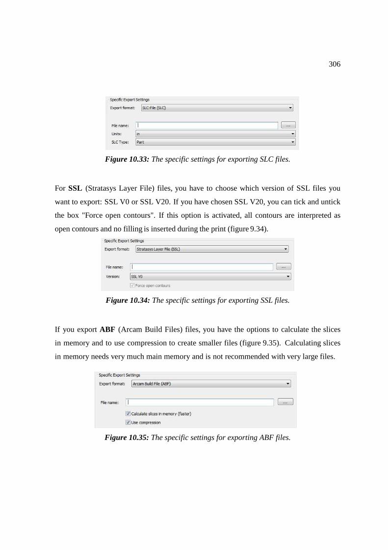
306
Figure 10.33: The specific settings for exporting SLC files.
For SSL (Stratasys Layer File) files, you have to choose which version of SSL files you
want to export: SSL V0 or SSL V20. If you have chosen SSL V20, you can tick and untick
the box "Force open contours". If this option is activated, all contours are interpreted as
open contours and no filling is inserted during the print (figure 9.34).
Figure 10.34: The specific settings for exporting SSL files.
If you export ABF (Arcam Build Files) files, you have the options to calculate the slices
in memory and to use compression to create smaller files (figure 9.35). Calculating slices
in memory needs very much main memory and is not recommended with very large files.
Figure 10.35: The specific settings for exporting ABF files.
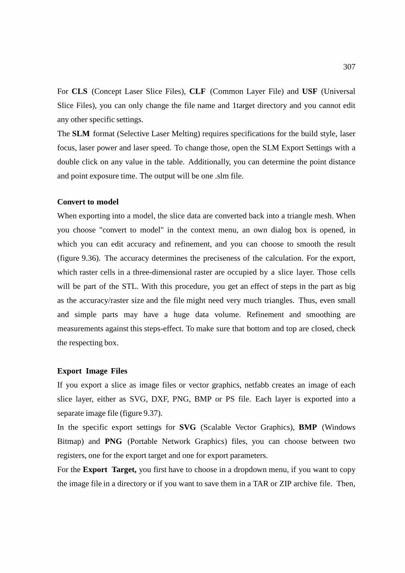
307
For CLS (Concept Laser Slice Files), CLF (Common Layer File) and USF (Universal
Slice Files), you can only change the file name and 1target directory and you cannot edit
any other specific settings.
The SLM format (Selective Laser Melting) requires specifications for the build style, laser
focus, laser power and laser speed. To change those, open the SLM Export Settings with a
double click on any value in the table. Additionally, you can determine the point distance
and point exposure time. The output will be one .slm file. Convert to model
When exporting into a model, the slice data are converted back into a triangle mesh. When
you choose "convert to model" in the context menu, an own dialog box is opened, in
which you can edit accuracy and refinement, and you can choose to smooth the result
(figure 9.36). The accuracy determines the preciseness of the calculation. For the export,
which raster cells in a three-dimensional raster are occupied by a slice layer. Those cells
will be part of the STL. With this procedure, you get an effect of steps in the part as big
as the accuracy/raster size and the file might need very much triangles. Thus, even small
and simple parts may have a huge data volume. Refinement and smoothing are
measurements against this steps-effect. To make sure that bottom and top are closed, check
the respecting box.
Export Image Files
If you export a slice as image files or vector graphics, netfabb creates an image of each
slice layer, either as SVG, DXF, PNG, BMP or PS file. Each layer is exported into a
separate image file (figure 9.37).
In the specific export settings for SVG (Scalable Vector Graphics), BMP (Windows
Bitmap) and PNG (Portable Network Graphics) files, you can choose between two
registers, one for the export target and one for export parameters.
For the Export Target, you first have to choose in a dropdown menu, if you want to copy
the image file in a directory or if you want to save them in a TAR or ZIP archive file. Then,
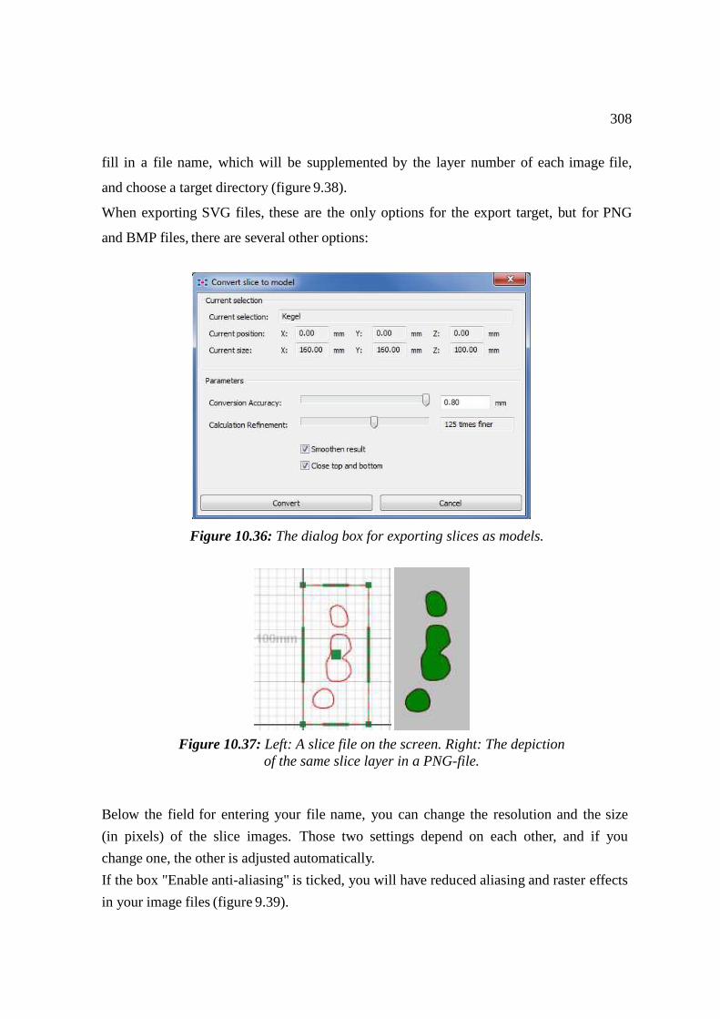
308
fill in a file name, which will be supplemented by the layer number of each image file,
and choose a target directory (figure 9.38).
When exporting SVG files, these are the only options for the export target, but for PNG
and BMP files, there are several other options:
Figure 10.36: The dialog box for exporting slices as models.
Below the field for entering your file name, you can change the resolution and the size
(in pixels) of the slice images. Those two settings depend on each other, and if you
change one, the other is adjusted automatically.
If the box "Enable anti-aliasing" is ticked, you will have reduced aliasing and raster effects
in your image files (figure 9.39).
Figure 10.37: Left: A slice file on the screen. Right: The depiction of the same slice layer in a PNG-file.
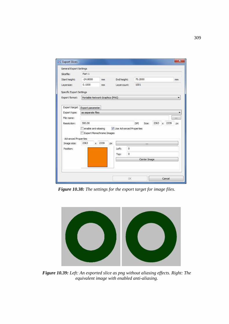
309
Figure 10.38: The settings for the export target for image files.
Figure 10.39: Left: An exported slice as png without aliasing effects. Right: The
equivalent image with enabled anti-aliasing.
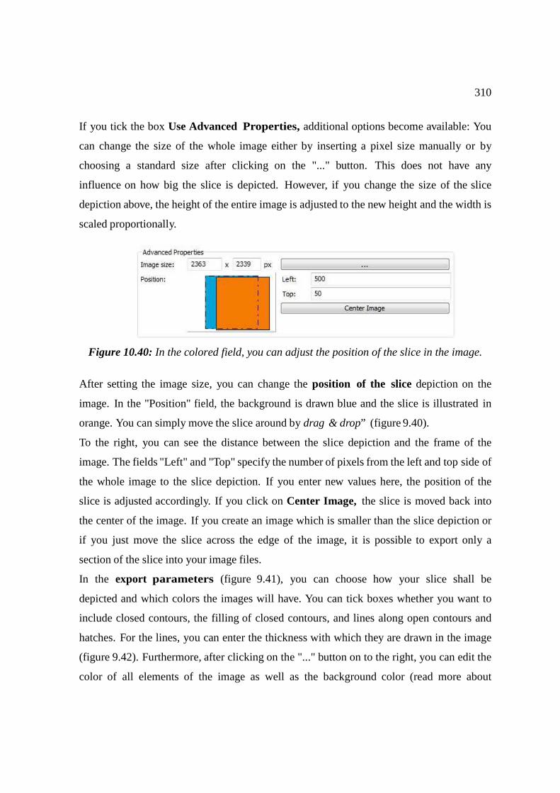
310
If you tick the box Use Advanced Properties, additional options become available: You
can change the size of the whole image either by inserting a pixel size manually or by
choosing a standard size after clicking on the "..." button. This does not have any
influence on how big the slice is depicted. However, if you change the size of the slice
depiction above, the height of the entire image is adjusted to the new height and the width is
scaled proportionally.
Figure 10.40: In the colored field, you can adjust the position of the slice in the image.
After setting the image size, you can change the position of the slice depiction on the
image. In the "Position" field, the background is drawn blue and the slice is illustrated in
orange. You can simply move the slice around by drag & drop” (figure 9.40).
To the right, you can see the distance between the slice depiction and the frame of the
image. The fields "Left" and "Top" specify the number of pixels from the left and top side of
the whole image to the slice depiction. If you enter new values here, the position of the
slice is adjusted accordingly. If you click on Center Image, the slice is moved back into
the center of the image. If you create an image which is smaller than the slice depiction or
if you just move the slice across the edge of the image, it is possible to export only a
section of the slice into your image files.
In the export parameters (figure 9.41), you can choose how your slice shall be
depicted and which colors the images will have. You can tick boxes whether you want to
include closed contours, the filling of closed contours, and lines along open contours and
hatches. For the lines, you can enter the thickness with which they are drawn in the image
(figure 9.42). Furthermore, after clicking on the "..." button on to the right, you can edit the
color of all elements of the image as well as the background color (read more about

311
changing colors in chapter 10.2). When you export SVG files, the filling and the
background are always white and cannot be changed.
Figure 10.41: The settings for the export parameters for image files.
Figure 10.42: Left: A slice image with grey background, where only the closed contour is visualized. Right: Here, the contour is filled and a different color is assigned.

312
For DXF (Drawing Interchange Format) files you can only choose to export either
separate files, a TAR archive or a ZIP archive in the dropdown menu and select a target
folder (figure 9.43).
Figure 10.43: The specific settings for exporting DXF files.
For PS (Adobe Postscript) files, all images are saved in one file, with one page per layer.
You can choose, if the inside or the outside of the slice is black (with the box "Inverted")
and you can choose either the portrait or the landscape page format as orientation (figure
9.44).
Figure 10.44: The specific settings for exporting PS files.

313
11 Settings
Settings for netfabb can be altered in the Settings menu. General settings concern all kinds
of aspects of the software, including the coloration of all visualizations, and can be
changed in a separate window, if you choose "Settings". If you click on "Edit File
Associations", you can choose which file types shall be linked to netfabb.
Figure 11.1: The settings menu
11.1 General Settings
The settings for netfabb can be changed in the Settings menu. After clicking on
"Settings", a window appears where settings for many different aspects of the
software can be altered (figure 10.2). The settings can either be changed in a dropdown
menu, by insertion of values or names, or by opening a dialog box with a double-click on
the current setting.
List of General Settings
Language:
Current available languages are English, German, Russian, Czech, Chinese, Japanese and
Spanish.
Unit of Length:
In this dropdown menu, you can choose between mm and inch as standard unit of length
for your netfabb installation.
314
Show Icons in Menu:
If you deactivate this option, no icons are shown in the menus and context menus of
netfabb. Shown icons are always to the left of the menu functions.
Proxy Settings:
In the proxy settings, you first have to choose, if you want to use admin settings or not. If
you do so, the settings can only be changed by the administrator in the admin settings at the
top. If not, you can change the proxy settings here.
You may need an internet connection for updates or accessing the netfabb online help. If your
internet connection is based on proxies, you can change your Proxy-Settings, Proxy-Server,
Proxy-Username and Proxy-Password in the respective fields. If you have a direct internet
connection, the other proxy settings are not necessary. If you have a Proxy server without
authentication, no username and password have to be entered.
License Settings:
If you have more than one license of netfabb, choose the one which you prefer to use.
• License type: for a floating license, choose “network license”
• Hostname/IP: enter the hostname OR the IP where your license is stored
• Backup Hostname/IP: enter the hostname OR the IP (the opposite of what you
chose above!) in order to have a backup if one of them is not available.
• Use add-ons: Choose which add-ons you want to use from your license. For
example: If your company has a license from a netfabb Professional with CAD
Import, but you only need the Professional, choose “No” in order to keep the
CAD Import available for your colleagues.
Activate netfabb Crash Logger:
If you run across any errors, the Crash Logger provides further information. A small extra
tool is required though, please contact [email protected].
Rotation with mouse, discretation degree:
When rotating manually, hold ALT and the part will be rotated by steps of this angle.
Rotation X, Y, Z degree:
When rotating by the x, y or z key the part will be rotated by steps of this angle.
315
Colors:
Set the colors for platform, parts and modules.
Default Platform size:
The size of the platform is best adjusted to the size of the build platform in your machine.
Zoom to newly created part:
Whenever you have created a part, the display will zoom into it.
Automatic check for erroneous parts:
If you do not always check for parts with errors, there will not be any warning signs, if you
have damaged or faulty parts in your project.
Import and export
Resolve Windows Link File Names:
This setting determines the naming of parts which are opened with a .lnk link file that
links to a 3D file. If it is inactive, the part in the project will be named as the .lnk file, if it
is active it will be named as the 3D file.
Ask for saving while deleting part:
If you remove a part, netfabb will ask if you’re sure about this.
Change LOD for all opened files:
All parts and project will automatically be opened with this value.
Restore LOD after Project Loading:
Whenever working with a lower Level of Detail in order to speed up processing, it’s
possible to save it and continue working with this LOD next time.
Confirm after project saving:
If this option is activated and you save a project, you’ll get a confirmation when the
process has been finished.
Always use file preview:
If you select "Yes", the File Preview Browser will start every time you want to open a file.
Use Advanced file import:
If this is activated, a dialog box appears where you can change the settings for the import
and stitch, scale and duplicate parts (see chapter 3.2.2).
316
Display Settings
Strength of background gradient:
In your background, there is a color gradient gradually changing from bright at the top of
the viewing screen to dark at the bottom of the viewing screen. The default color is white,
which becomes grey at the bottom.
Use enhanced display functions (OpenGL3.3):
The enhanced display functions enables a prettier rendering of the parts. If you have
troubles with displaying your parts, set this function to No.
Level of detail:
Use the simple mode for quicker calculation or the advanced mode for a more precise view
of the part.
Highlight center of platform:
If you choose Yes, a large X will indicate the center of the platform.
Coordinate System:
The coordinate system in the bottom left of the viewing screen, can be altered in size. If
the planes are shown, their minimum and maximum size, as well as their thickness can be
specified. The size of the planes in the program varies between the minimum and
maximum value, depending on the current perspective, with planes in the background
always displayed larger than those in the foreground. The planes, if displayed, can be used
for changing the perspective.
Slice Commander
In case you visualize the prehatches of slices with the option Show Filling (chapter
9.4.2), you can edit the distance of the grid lines here. Additionally, you can choose if you
want to have grid lines along the X-axis, the Y-axis or along both axes (figure 10.4). Also,
you can edit the default tolerance for point reductions (chapter 9.5.3). You can also edit
the tolerance at every single point reduction.

317
Figure 11.2: The prehatches of a slice with grid lines along both axes (left) and grid lines only along Y-axis (right).
Parts Library
In the Parts Library Section, you can edit the default settings for all parameters of all
primitive objects you can add to the project (see chapter 5.3).
Part Repair
For the part repair (figure 10.5), it is possible to change the default stitch tolerance. You do
not necessarily have to use that value for the stitching of triangles, as you can set the
tolerance for every single stitching.
The minimum edge length for good faces determines which triangles are defined as
"degenerated" in the repair module. All triangles with a height lower than this value can
be displayed in orange and are deleted with the function Remove degenerate faces (see
chapter 7.5.7) the orange highlighting of degenerate triangles in the repair module.
Triangles with an edge shorter than the specified value are marked (figure 10.5).
Figure 11.3: The settings for the repair module.
Measuring
For the measuring, you can choose in dropdown menus, which measuring mode and which
option for setting anchor points shall be set when you start the measuring module.
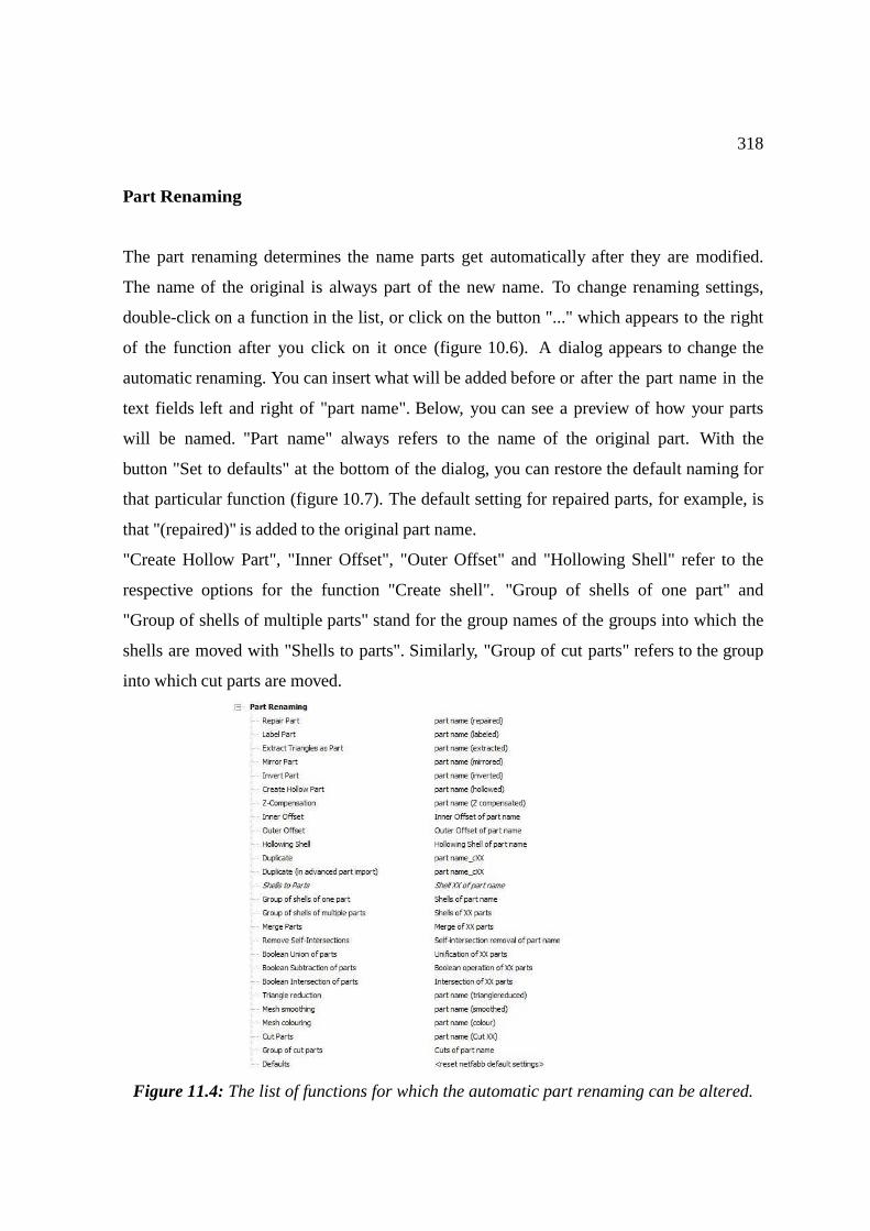
318
Part Renaming
The part renaming determines the name parts get automatically after they are modified.
The name of the original is always part of the new name. To change renaming settings,
double-click on a function in the list, or click on the button "..." which appears to the right
of the function after you click on it once (figure 10.6). A dialog appears to change the
automatic renaming. You can insert what will be added before or after the part name in the
text fields left and right of "part name". Below, you can see a preview of how your parts
will be named. "Part name" always refers to the name of the original part. With the
button "Set to defaults" at the bottom of the dialog, you can restore the default naming for
that particular function (figure 10.7). The default setting for repaired parts, for example, is
that "(repaired)" is added to the original part name.
"Create Hollow Part", "Inner Offset", "Outer Offset" and "Hollowing Shell" refer to the
respective options for the function "Create shell". "Group of shells of one part" and
"Group of shells of multiple parts" stand for the group names of the groups into which the
shells are moved with "Shells to parts". Similarly, "Group of cut parts" refers to the group
into which cut parts are moved.
Figure 11.4: The list of functions for which the automatic part renaming can be altered.
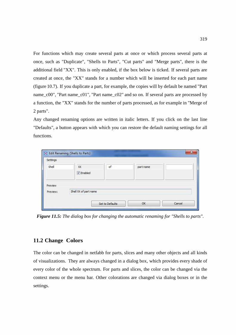
319
For functions which may create several parts at once or which process several parts at
once, such as "Duplicate", "Shells to Parts", "Cut parts" and "Merge parts", there is the
additional field "XX". This is only enabled, if the box below is ticked. If several parts are
created at once, the "XX" stands for a number which will be inserted for each part name
(figure 10.7). If you duplicate a part, for example, the copies will by default be named "Part
name_c00", "Part name_c01", "Part name_c02" and so on. If several parts are processed by
a function, the "XX" stands for the number of parts processed, as for example in "Merge of
2 parts".
Any changed renaming options are written in italic letters. If you click on the last line
"Defaults", a button appears with which you can restore the default naming settings for all
functions.
Figure 11.5: The dialog box for changing the automatic renaming for "Shells to parts".
11.2 Change Colors
The color can be changed in netfabb for parts, slices and many other objects and all kinds
of visualizations. They are always changed in a dialog box, which provides every shade of
every color of the whole spectrum. For parts and slices, the color can be changed via the
context menu or the menu bar. Other colorations are changed via dialog boxes or in the
settings.
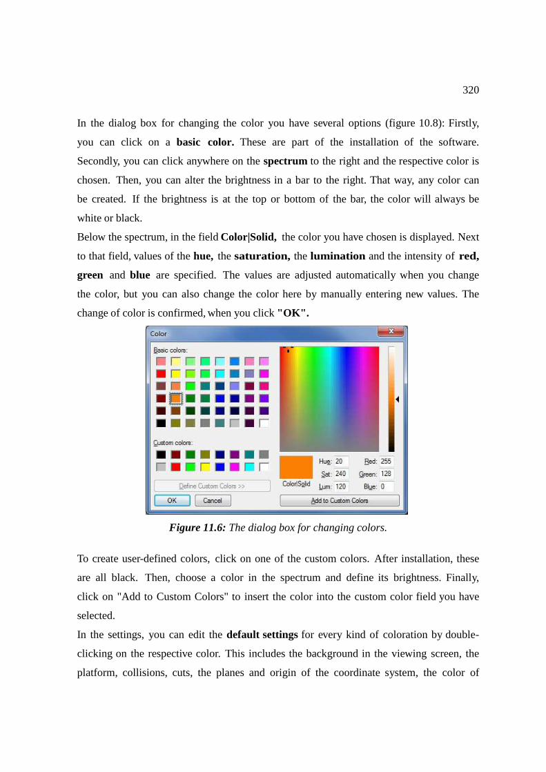
320
In the dialog box for changing the color you have several options (figure 10.8): Firstly,
you can click on a basic color. These are part of the installation of the software.
Secondly, you can click anywhere on the spectrum to the right and the respective color is
chosen. Then, you can alter the brightness in a bar to the right. That way, any color can
be created. If the brightness is at the top or bottom of the bar, the color will always be
white or black.
Below the spectrum, in the field Color|Solid, the color you have chosen is displayed. Next
to that field, values of the hue, the saturation, the lumination and the intensity of red,
green and blue are specified. The values are adjusted automatically when you change
the color, but you can also change the color here by manually entering new values. The
change of color is confirmed, when you click "OK".
Figure 11.6: The dialog box for changing colors.
To create user-defined colors, click on one of the custom colors. After installation, these
are all black. Then, choose a color in the spectrum and define its brightness. Finally,
click on "Add to Custom Colors" to insert the color into the custom color field you have
selected.
In the settings, you can edit the default settings for every kind of coloration by double-
clicking on the respective color. This includes the background in the viewing screen, the
platform, collisions, cuts, the planes and origin of the coordinate system, the color of
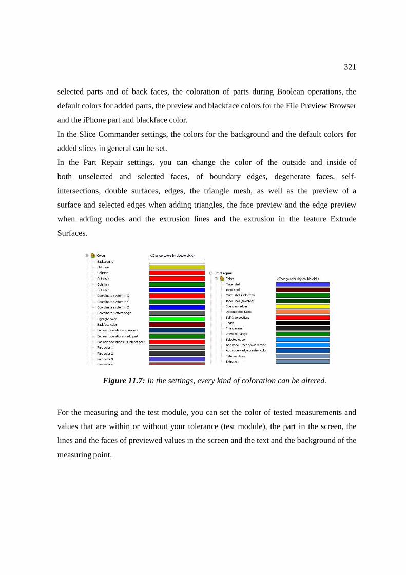
321
selected parts and of back faces, the coloration of parts during Boolean operations, the
default colors for added parts, the preview and blackface colors for the File Preview Browser
and the iPhone part and blackface color.
In the Slice Commander settings, the colors for the background and the default colors for
added slices in general can be set.
In the Part Repair settings, you can change the color of the outside and inside of
both unselected and selected faces, of boundary edges, degenerate faces, self-
intersections, double surfaces, edges, the triangle mesh, as well as the preview of a
surface and selected edges when adding triangles, the face preview and the edge preview
when adding nodes and the extrusion lines and the extrusion in the feature Extrude
Surfaces.
For the measuring and the test module, you can set the color of tested measurements and
values that are within or without your tolerance (test module), the part in the screen, the
lines and the faces of previewed values in the screen and the text and the background of the
measuring point.
Figure 11.7: In the settings, every kind of coloration can be altered.
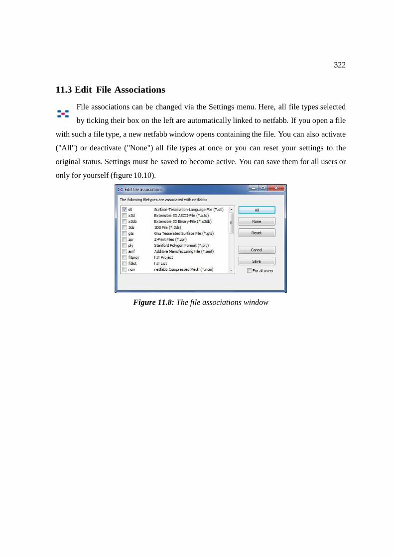
322
11.3 Edit File Associations
File associations can be changed via the Settings menu. Here, all file types selected
by ticking their box on the left are automatically linked to netfabb. If you open a file
with such a file type, a new netfabb window opens containing the file. You can also activate
("All") or deactivate ("None") all file types at once or you can reset your settings to the
original status. Settings must be saved to become active. You can save them for all users or
only for yourself (figure 10.10).
Figure 11.8: The file associations window
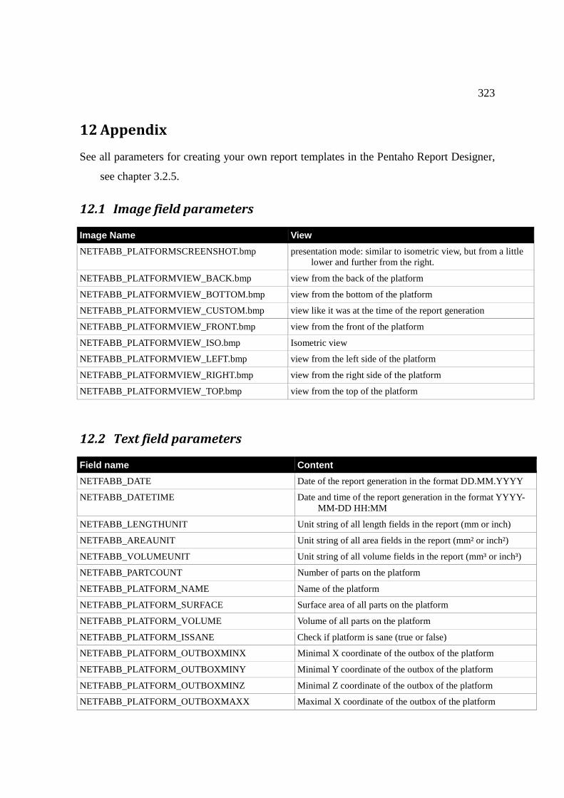
323
12 Appendix
See all parameters for creating your own report templates in the Pentaho Report Designer,
see chapter 3.2.5.
12.1 Image field parameters
Image Name View
NETFABB_PLATFORMSCREENSHOT.bmp presentation mode: similar to isometric view, but from a little lower and further from the right.
NETFABB_PLATFORMVIEW_BACK.bmp view from the back of the platform
NETFABB_PLATFORMVIEW_BOTTOM.bmp view from the bottom of the platform
NETFABB_PLATFORMVIEW_CUSTOM.bmp view like it was at the time of the report generation
NETFABB_PLATFORMVIEW_FRONT.bmp view from the front of the platform
NETFABB_PLATFORMVIEW_ISO.bmp Isometric view
NETFABB_PLATFORMVIEW_LEFT.bmp view from the left side of the platform
NETFABB_PLATFORMVIEW_RIGHT.bmp view from the right side of the platform
NETFABB_PLATFORMVIEW_TOP.bmp view from the top of the platform
12.2 Text field parameters
Field name Content
NETFABB_DATE Date of the report generation in the format DD.MM.YYYY
NETFABB_DATETIME Date and time of the report generation in the format YYYY-MM-DD HH:MM
NETFABB_LENGTHUNIT Unit string of all length fields in the report (mm or inch)
NETFABB_AREAUNIT Unit string of all area fields in the report (mm² or inch²)
NETFABB_VOLUMEUNIT Unit string of all volume fields in the report (mm³ or inch³)
NETFABB_PARTCOUNT Number of parts on the platform
NETFABB_PLATFORM_NAME Name of the platform
NETFABB_PLATFORM_SURFACE Surface area of all parts on the platform
NETFABB_PLATFORM_VOLUME Volume of all parts on the platform
NETFABB_PLATFORM_ISSANE Check if platform is sane (true or false)
NETFABB_PLATFORM_OUTBOXMINX Minimal X coordinate of the outbox of the platform
NETFABB_PLATFORM_OUTBOXMINY Minimal Y coordinate of the outbox of the platform
NETFABB_PLATFORM_OUTBOXMINZ Minimal Z coordinate of the outbox of the platform
NETFABB_PLATFORM_OUTBOXMAXX Maximal X coordinate of the outbox of the platform
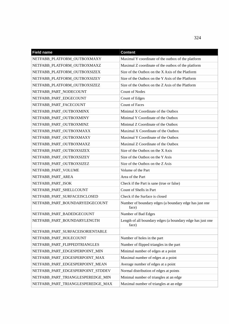
324
Field name Content
NETFABB_PLATFORM_OUTBOXMAXY Maximal Y coordinate of the outbox of the platform
NETFABB_PLATFORM_OUTBOXMAXZ Maximal Z coordinate of the outbox of the platform
NETFABB_PLATFORM_OUTBOXSIZEX Size of the Outbox on the X Axis of the Platform
NETFABB_PLATFORM_OUTBOXSIZEY Size of the Outbox on the Y Axis of the Platform
NETFABB_PLATFORM_OUTBOXSIZEZ Size of the Outbox on the Z Axis of the Platform
NETFABB_PART_NODECOUNT Count of Nodes
NETFABB_PART_EDGECOUNT Count of Edges
NETFABB_PART_FACECOUNT Count of Faces
NETFABB_PART_OUTBOXMINX Minimal X Coordinate of the Outbox
NETFABB_PART_OUTBOXMINY Minimal Y Coordinate of the Outbox
NETFABB_PART_OUTBOXMINZ Minimal Z Coordinate of the Outbox
NETFABB_PART_OUTBOXMAXX Maximal X Coordinate of the Outbox
NETFABB_PART_OUTBOXMAXY Maximal Y Coordinate of the Outbox
NETFABB_PART_OUTBOXMAXZ Maximal Z Coordinate of the Outbox
NETFABB_PART_OUTBOXSIZEX Size of the Outbox on the X Axis
NETFABB_PART_OUTBOXSIZEY Size of the Outbox on the Y Axis
NETFABB_PART_OUTBOXSIZEZ Size of the Outbox on the Z Axis
NETFABB_PART_VOLUME Volume of the Part
NETFABB_PART_AREA Area of the Part
NETFABB_PART_ISOK Check if the Part is sane (true or false)
NETFABB_PART_SHELLCOUNT Count of Shells in Part
NETFABB_PART_SURFACEISCLOSED Check if the Surface is closed
NETFABB_PART_BOUNDARYEDGECOUNT Number of boundary edges (a boundary edge has just one face)
NETFABB_PART_BADEDGECOUNT Number of Bad Edges
NETFABB_PART_BOUNDARYLENGTH Length of all boundary edges (a boundary edge has just one face)
NETFABB_PART_SURFACEISORIENTABLE
NETFABB_PART_HOLECOUNT Number of holes in the part
NETFABB_PART_FLIPPEDTRIANGLES Number of flipped triangles in the part
NETFABB_PART_EDGESPERPOINT_MIN Minimal number of edges at a point
NETFABB_PART_EDGESPERPOINT_MAX Maximal number of edges at a point
NETFABB_PART_EDGESPERPOINT_MEAN Average number of edges at a point
NETFABB_PART_EDGESPERPOINT_STDDEV Normal distribution of edges at points
NETFABB_PART_TRIANGLESPEREDGE_MIN Minimal number of triangles at an edge
NETFABB_PART_TRIANGLESPEREDGE_MAX Maximal number of triangles at an edge
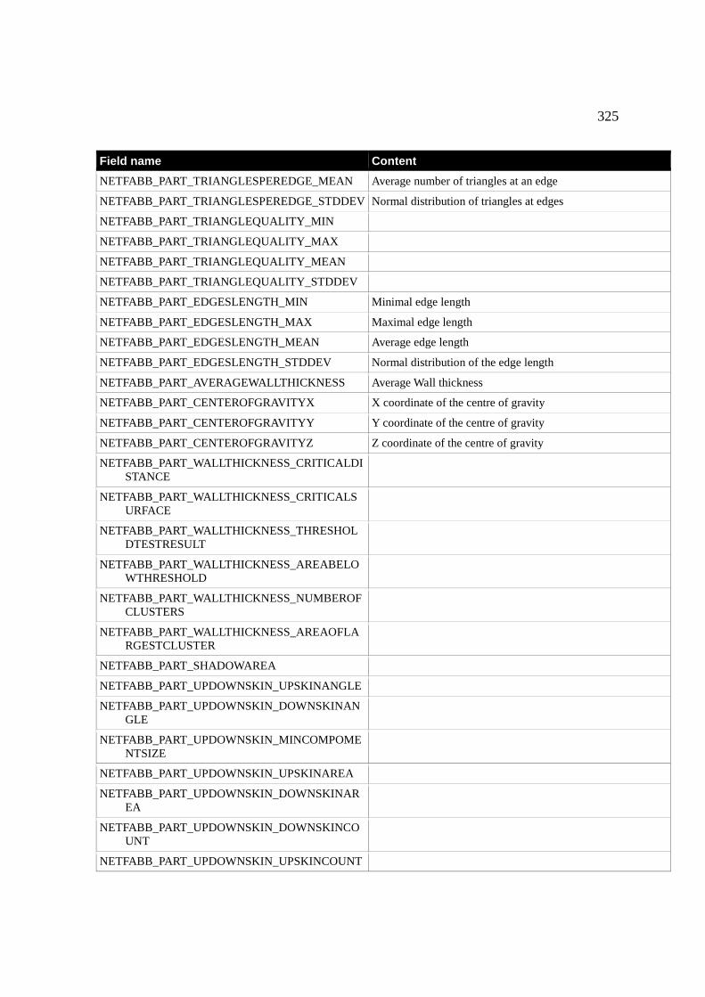
325
Field name Content
NETFABB_PART_TRIANGLESPEREDGE_MEAN Average number of triangles at an edge
NETFABB_PART_TRIANGLESPEREDGE_STDDEV Normal distribution of triangles at edges
NETFABB_PART_TRIANGLEQUALITY_MIN
NETFABB_PART_TRIANGLEQUALITY_MAX
NETFABB_PART_TRIANGLEQUALITY_MEAN
NETFABB_PART_TRIANGLEQUALITY_STDDEV
NETFABB_PART_EDGESLENGTH_MIN Minimal edge length
NETFABB_PART_EDGESLENGTH_MAX Maximal edge length
NETFABB_PART_EDGESLENGTH_MEAN Average edge length
NETFABB_PART_EDGESLENGTH_STDDEV Normal distribution of the edge length
NETFABB_PART_AVERAGEWALLTHICKNESS Average Wall thickness
NETFABB_PART_CENTEROFGRAVITYX X coordinate of the centre of gravity
NETFABB_PART_CENTEROFGRAVITYY Y coordinate of the centre of gravity
NETFABB_PART_CENTEROFGRAVITYZ Z coordinate of the centre of gravity
NETFABB_PART_WALLTHICKNESS_CRITICALDISTANCE
NETFABB_PART_WALLTHICKNESS_CRITICALSURFACE
NETFABB_PART_WALLTHICKNESS_THRESHOLDTESTRESULT
NETFABB_PART_WALLTHICKNESS_AREABELOWTHRESHOLD
NETFABB_PART_WALLTHICKNESS_NUMBEROFCLUSTERS
NETFABB_PART_WALLTHICKNESS_AREAOFLARGESTCLUSTER
NETFABB_PART_SHADOWAREA
NETFABB_PART_UPDOWNSKIN_UPSKINANGLE
NETFABB_PART_UPDOWNSKIN_DOWNSKINANGLE
NETFABB_PART_UPDOWNSKIN_MINCOMPOMENTSIZE
NETFABB_PART_UPDOWNSKIN_UPSKINAREA
NETFABB_PART_UPDOWNSKIN_DOWNSKINAREA
NETFABB_PART_UPDOWNSKIN_DOWNSKINCOUNT
NETFABB_PART_UPDOWNSKIN_UPSKINCOUNT