Embed Size (px)
Citation preview

DI
SC
US
SI
ON
P
AP
ER
S
ER
IE
S
Forschungsinstitut zur Zukunft der ArbeitInstitute for the Study of Labor
Neighborhood Quality and Student Performance
IZA DP No. 7139
January 2013
Felix Weinhardt

Neighborhood Quality and
Student Performance
Felix Weinhardt London School of Economics (CEE, CEP, SERC)
and IZA
Discussion Paper No. 7139 January 2013
IZA
P.O. Box 7240 53072 Bonn
Germany
Phone: +49-228-3894-0 Fax: +49-228-3894-180
E-mail: [email protected]
Any opinions expressed here are those of the author(s) and not those of IZA. Research published in this series may include views on policy, but the institute itself takes no institutional policy positions. The IZA research network is committed to the IZA Guiding Principles of Research Integrity. The Institute for the Study of Labor (IZA) in Bonn is a local and virtual international research center and a place of communication between science, politics and business. IZA is an independent nonprofit organization supported by Deutsche Post Foundation. The center is associated with the University of Bonn and offers a stimulating research environment through its international network, workshops and conferences, data service, project support, research visits and doctoral program. IZA engages in (i) original and internationally competitive research in all fields of labor economics, (ii) development of policy concepts, and (iii) dissemination of research results and concepts to the interested public. IZA Discussion Papers often represent preliminary work and are circulated to encourage discussion. Citation of such a paper should account for its provisional character. A revised version may be available directly from the author.
IZA Discussion Paper No. 7139 January 2013
ABSTRACT
Neighborhood Quality and Student Performance1 Children who grow up in deprived neighborhoods underperform at school and later in life but whether there is a causal link remains contested. This study estimates the effect of very deprived neighborhoods, characterized by a high density of social housing, on the educational attainment of fourteen years old students in England. To identify the causal impact, this study exploits the timing of moving into these neighborhoods. I argue that the timing can be taken as exogenous because of long waiting lists for social housing in high-demand areas. Using this approach, I find no evidence for effects on student performance. JEL Classification: J18, I21, J24 Keywords: neighborhood effects, housing policy Corresponding author: Felix Weinhardt Centre for Economic Performance (CEP) London School of Economics Houghton Street London, WC2A 2AE United Kingdom E-mail: [email protected]
1 ESRC funding gratefully acknowledged (Ref: ES/F022166/1, ES/J003867/1). Helpful comments from Sascha Becker, Thomas Breda, Christian Hilber, Ifty Hussain, Victor Lavy, Tim Leunig, Alan Manning, Richard Murphy, Henry Overman, Frédéric Robert-Nicoud, Stephen Ross, Olmo Silva, Petra Todd, and Yves Zenou, and participants of the EALE/SOLE conference in London, the NARSC Urban Economics Association Conference in San Francisco, the Spatial Econometrics Conference in Barcelona, the LSE-SERC Urban Economics Seminar, the LSE-CEP Labour Market Workshop, the 2010 IZA Summer School, the 2010 ZEW Workshop on “Evaluation of Policies Fighting Social Exclusion”; and the CEP-CEE Education Workshop are gratefully acknowledged. Previous working paper version: Weinhardt (2010). I declare that I have no relevant or material financial interest that relate to the research described in this paper. All remaining errors are my own.

2
I.Introduction
Children who grow up in deprived neighborhoods underperform at school and later in
life. In England, the most deprived neighborhoodshave high concentrations of social
housing (public housing)and are characterized by very high unemployment and extremely
low qualification rates, high building density, over-crowding and low house
prices.Growing up in social housing is associated with unfavorable outcomes:adults who
lived in social housing during their childhood are more likely to be depressed,
unemployed, cigarette smokers, obese, and have lower qualification levels compared to
peers in their cohort who never lived in social housing (Lupton et al. 2009). The following
concern arises: if living in a bad neighborhood has direct negative effects on outcomes
such as school results, this could in extreme cases constitute a locking-in of the
disadvantaged into a spatial poverty trap: ‘once you get into a bad neighborhood, you and
your children
won’t get out’2. In a society that believes that everyone deserves a fair chance, it is hence
not surprising that this disadvantageassociated to deprived neighborhoods has attracted
attention from researchers and policymakers alike3.
This paper establishes whether moving into localized high-density social housing
neighborhoods causes a deterioration in the school attainment of fourteen-year-old
students. The English setting offers a unique opportunity to answer this research question
for two reasons.
Firstly, the geographical sorting problem needs to be overcome, which otherwise
induces spurious correlations between individual and neighbors’ outcomes (Manski, 1993,
Moffitt 2001). In order to identify the causal impact of neighborhood deprivation on
student attainment this study exploits the timing of moving into these neighborhoods
around the national age-fourteen Key Stage 3 (KS3) exam. In England, the timing of a
move can be taken as exogenous because of long waiting lists for social housing in high-
demand areas. In these areas, waiting times can exceed ten years, and I argue that we can
2 This might be the case because of peer group and role model effects (Akerlof 1997; Glaeser and Scheinkman
2001), social networks (Granovetter 1995; Calvó-Armengol and Jackson 2004; Bayer et al. 2008; Zenou 2008; Small 2009; Figlio et al. 2011), conformism (Bernheim 1994; Fehr and Falk 2002) or local resources such as school quality or other environmental (Durlauf 1996, Lupton 2005). It is not the aim of this paper to distinguish between these theoretical channels.
3Housing policies that rest on the idea of a causal channel from the place of residence to individual outcomes are
inclusionary zoning and desegregation policies, as well as regeneration and mixed-housing projects, such as ‘Hope VI’ in the US, or the ‘mixed communities’ initiative in England (e.g. Cheshire et al. 2008).

3
therefore compare test scores of students who experience large deteriorations in
neighborhood quality before the exam, to test scores of other pupils who will be
subjected to the same neighborhood treatment in the future (Figure 1). Naturally, a
student’s result in the KS3 exam can only be influenced by the low quality of her new
neighborhood if she moves into this neighborhood before taking the test. Later movers
only receive a (future) ‘placebo’ treatment and serve as natural control group as they are
likely to share many unobserved characteristics common to social tenants4. We know that
pupils from deprived family backgrounds are prioritized, but identification only relies on
them being prioritized in a similar way before and after the KS3 test. This means that we
can relax the usual assumption that social housing neighborhood allocation is quasi-
random as such (e.g. Oreopoulos 2003). Time-invariant preferences or unobserved
institutional arrangements that could give rise to neighborhood sorting can be captured
by the neighborhood fixed effect. The remaining assumption required for identification is
that allocation and individual sorting preferences for particular neighborhoods do not
change over the study period. In support of this assumption, I show that a rich set of
individual characteristics fails to predict the time of the move. I interpret this as direct
evidence in favor of the validity of the identification assumption of quasi-random timing.
Secondly, nation-wide census data makes it possible to track individual residential
mobility for two cohorts of students in England; the study is therefore not limited to a
small number of neighborhoods or of cities. The richness of the data also allows
including controls for a potential direct effect of moving, earlier attainment, family
background and school quality.
The main finding of this study is that early movers into deprived social housing
neighborhoods experience no negative effects on their school attainment relative to late
movers. While it is demonstrated that there are large negative associations between
moving into deprived areas and school outcomes, these negative correlations cease to
4This strategy is related to Rothstein (2010) who studies effects of teacher quality and exploits the fact that future
teachers cannot affect contemporaneous value added test scores.
FIGURE 1: KS3 DISCONTINUITY
4
exist once controlling for group-specific observable and unobservable characteristics in a
difference-in-difference framework.
To the best of the author’s knowledge, exploiting the timing of moving when waiting
lists are long is a novel strategy to study neighborhood effects.5 Besides this
methodological innovation, the finding of no effects on school outcomes from moving
into high-density social housing projects informs the literature. For educational outcomes,
the only existing experimental study, the Moving to Opportunity (MTO) intervention, a
mobility voucher scheme, finds little evidence for neighborhood effects in both the short
and the long-run (Katz et al. 2001, Sanbonmatsuet al. 2006, Kling et al. 2007, Ludwig et al.
2012). However, the MTO has been questioned by some because of its focus on relatively
small neighborhood-level changes (i.e. small ‘treatments’) and limited geographical
representativeness (Quigley and Raphael 2008, Clampet-Lunquist and Massey 2008, Small
and Feldman 2012). Furthermore, the non-experimental literature tends to find evidence
in favor of neighborhood effects on educational outcomes, which is the opposite of the
MTO. Goux and Maurin (2007) study the effect of close neighbors in France and find
strong effects on end of junior high-school performance and Card and Rothstein (2007)
find effects of city-level racial segregation on the black-white test score gap6.To the
author’s knowledge, this is the first non-experimental study that does not find evidence
for short-term effects on school outcomes from highly deprived neighborhoods, thus
supporting the conclusions from the experimental literature.
The rest of the paper is structured as follows: The next section describes the empirical
strategy, section III the institutional setting and the data; Section IV discusses the results;
and Section V presents a battery of robustness checks before I conclude.
5 Existing research used instrumental variables (Cutler and Glaeser 1997, Goux and Maurin 2007); aggregation
(Card and Rothstein 2007); institutional settings (Oreopoulos 2003, Jacob 2004, Gould et al. 2004, Gurmuet al. 2007, Goux and Maurin 2007); fixed effects (Aaronson 1998, Bayer et al. 2009, Gibbons et al. 2011) or experimental setups (Katz et al. 2001, 2007, Sanbonmatsuet al. 2006, Ludwig et al. 2012).
6In another paper Jacob (2004) does not find effects of public housing demolitions on student achievement, but
in his setting students move between very similar neighborhoods so he is not testing for neighborhood effects but an independent effect of public housing. In addition, there is a related literature that shows that peers matter in school (i.e. Sacerdote 2001, Carrell et al. 2009, Lavy et al. 2012), and that neighborhoods matter for labor market outcomes (Cuter and Glaeser 1997, Ross 1998, Ananat 2007, Weinberg 2000, 2004, Bayer et al. 2008), although again the MTO and Oreopoulos (2003) do not find evidence for neighborhood effects on labor market outcomes. For a full review of the related literature see Ross (2011).
5
II.Empirical strategy
This study focusses on identifying the effect on educational attainment of moving into
high-density social housing neighborhoods. We know that people sort into their
neighborhoods along socio-demographic characteristics, which could induce spurious
correlations between neighborhood characteristics and pupil outcomes if unobserved
(Manski 1993, Moffitt 2001). Any study that makes causal claims about the relationship
between neighborhood characteristics and individual outcomes needs to present a
strategy to overcome this sorting problem. The focus of this study is on pupils who move
into social housing neighborhoods, the worry is hence that these pupils carry unobserved
characteristics that explain their educational underperformance and are also linked with
the fact that their parents got admitted into social housing in the first place. These factors
would generate spurious correlations between neighborhood characteristics and individual
outcomes even in the absence of any neighborhood effects.
As a novel strategy, this study exploits the timing of the move to control for all
observed and unobserved factors that are common to pupils moving into high density
social housing neighborhoods. Figure 2 illustrates this identification strategy. The time
when the Key Stage 3 (KS3) exam, a national and externally marked test, is taken is
denoted by t . The time for the national and externally marked Key Stage 2 (KS2) exam
by t -1 . t -1 to t span the English academic years seven to nine. This is equivalent to 6th
to 8th grade in the US context, more details on institutional background are given in
section III. Conversely, tand t 1+ cover the academic years ten and eleven after the KS3
(9th and 10th grade in the US). We can now compare test score value added of pupils who
move into deprived social housing neighborhoods before taking the KS3 test, in the
period from t -1 to t , to pupils who also move into deprived social housing
neighborhoods, but after sitting the KS3 exam in the period between t and t 1+ . The
latter group only received a ‘placebo’ treatment as the future neighborhood cannot affect
test scores of the test taken at time t and thus serves as control group. This group is likely
to share many–potentially unobserved- characteristics common to all pupils who move
into high-density social housing neighborhoods.7
7A further problem in neighborhoods effects research is the “reflection problem”. This issue arises because
individuals might not only be affected by other individuals in their neighborhood but might equally affect these themselves (Manski 1993). If neighborhood effects exit, this causes a reverse causality problem that upward biases the

6
A. The production function of educational attainment in the neighborhood
Formally, assume that test scores can be modeled as a linear function of neighborhood,
school and individual characteristics in the following way:
' ' ' ' 'ignsct nt it it c c ignsct
y t t c c tβ κ ε= + + + + + + +Z x γ x δ S φ S (1.1)
where ignscty denotes test scores of individual i of group g, in neighborhood n, school s,
cohort c in year t . ntZ denotes time-varying neighborhood characteristics that could
influence attainment at school, like the absence of role models, etc. The vector x denotes
individual-level characteristics that affect test scores, like family background
characteristics or earlier test scores. I further allow these characteristics to have a time-
varying effect on test outcomes, denoted by 'it
tx δ . The matrix S denotes school-level
characteristics and callows for different intercepts for the different cohorts, and both
could have effects depending on the timing, as well.
Further, let us assume that the error term contains the following elements:
ignsct i n n s s g g ignsctz z t s s t t eε α φ φ= + + + + + + +
(1.2)
Where i
α represents unobserved individual effects such as motivation, n
z unobserved
neighborhood characteristics,s
s unobserved year school quality and gφ unobserved
characteristics of belonging to group g . I think of g as representing time-invariant
characteristics which are common to pupils who move into social housing
neighborhoods. I further allow the unobserved neighborhood, school and group
characteristics to have time-varying effects through n
z t , s
s t and gtφ . Lastly, ignsct
e is the
error term which we assume to be random. The problem is that all former components
might correlate with individual and neighborhood specific variables from equation (1) for
the discussed reasons and hence bias any estimates.
The first step to potentially overcome these problems is to difference the equation:
1 1 1( ) ( ) ' ' ' ( )ignsct ignsct nt nt i c ignsct ignsct
y y cβ δ κ ε ε− − −− = − + + + + −Z Z x S (2.1)
neighborhood coefficients. Since this study finds no effects once we control for unobserved effects of moving into social housing, we do not need to be concerned with the reflection problem.

7
Where 1( )ignsct ignsct
y y −− is the test-score value added between KS2 and KS3 modeled
as a function of changes in the neighborhood environment 1( )nt nt−−Z Z , individual
characteristics i
x and school-characteristics S that affect value-added. Note that the time-
independent effects of individual characteristics, belonging to a particular cohort and of
the matrix of school variables all cancel out.
The differenced error term now has the following components:
1( )ignsct ignsct n g s ignsct
z s vε ε φ−− = + + + (2.2)
All time-invariant unobserved characteristics of equation (1.2) that do not have a time-
varying effect cancel out. What is left are the unobserved neighborhood characteristics
that could affect value added n
z , the group effects that have a time-varying effect φ ,
unobserved school-level variables that affect value-added s
s and ignsctv , which I assume to
be random. Note that I will cluster the error term at the neighborhood-level to allow for
local correlations in the error term matrix. Compared to (1.2), this differenced error term
does not contain any unobserved characteristics that affect test score levels. In some of
my regressions I can include fixed effects to control for two of the remaining three non-
random unobserved components gz , and
ss .
From an identification point of view this model is preferable to the levels-model
presented earlier. This is because all unobserved constant factors, in particular family
background or individual motivation, are now controlled for and can therefore not
generate spurious correlations through the sorting mechanism. Furthermore, by including
fixed effects for neighborhoods and schools any unobserved constant local factors
affecting value-added can be taken care of. This means that any constant unobserved
neighborhood or school characteristics can be captured and hence cannot induce
spurious correlations between neighborhood quality changes and test score progress.
However, a remaining worry is that pupils who move into social housing share individual
or background characteristics that are unobserved and correlate with neighborhood
changes. These unobserved group characteristics are captured by gφ in equation (2.2) and
cannot be directly controlled for. As I outlined in the beginning of this section, my

8
strategy addresses this final concern by comparing early movers to late movers8, so pupils
who experienced a neighborhood level treatment before sitting the KS3 exam at time t to
pupils who moved later and hence only received a ‘placebo’ treatment as future
neighborhood changes cannot affect past value added.
In order to mirror the setup from Figure 2 and to compare pupils who moved before
taking the test to the placebo group of pupils who moved into high-density social housing
neighborhoods only after sitting the KS3 test at time t in a regression framework, we need
to define indicator variables for moving into a high-density social housing neighborhood:
if pupil moves into social housing between and
0 otherwise i,t,t -1
= 1 t t -1D(SH)
=
if pupil moves into social housing between and
0 otherwise i,t,t+1
= 1 t t 1D(SH)
=
+
if pupil moves into social housing between and
0 otherwise i,t-1,t+1
= 1 t -1 t 1D(SH)
=
+
I use these indicator variables to proxy for neighborhood quality changes 1( )nt nt−−Z Z ,
as a catch-all proxy for the large deteriorations in neighborhood quality these pupils
experience (discussed in detail in sectionIII C).
One concern is that a move might also directly affect value added, and not only
indirectly through the change in neighborhood quality. The ‘placebo’ group only moves
after taking the test so that the neighborhood quality change cannot affect test scores, but
equally they don’t move before taking the test. If there was a direct effect of mobility on
test scores, i.e. through disruption, this could bias the estimates. To allay these concerns I
will difference out the pure effect of moving using the population of pupils who move
but not into social housing. To do this, let’s define the following sets:
if pupil moves between and
0 otherwise i,t,t -1
= 1 t t -1D(M)
=
8 I follow the literature (i.e. Katz et al. 2001, Jacob 2004) and rely on pupils who move to generate variation in the neighborhood
variables 1( )nt nt
z z −− , since neighborhoods change very slowly over time.

9
if pupil moves between and
0 otherwise i,t,t 1
= 1 t t 1D(M)
=+
+
if pupil moves between and
0 otherwise i,t -1,t+1
= 1 t -1 t 1D(M)
=
+
Finally, in the value-added model (2.1) we assume that past test scores predict today’s
test scores with an coefficient of one. I relax this assumption and instead of differencing
test scores manually on the left-hand-side include past test-scores as control variable on
the right-hand side of the equation. There is a worry that the coefficient on the past test
score will be downward biased if the KS2 test only measures ability with an error (see
Todd and Wolpin 2003). In this application however the way we control for past test
scores –or if we control for past test scores at all- makes little difference to the estimates.
This is because the placebo group is extremely similar to the treatment group, which I
come back to in section V.
With these ingredients we can now construct a difference-in-difference estimate from
equations (2.1) and (2.2) using the indicator variables defined above. To see this, let us
first set up a model for pupils who moved into high-density social housing
neighborhoods between time t -1 and t . Substituting the indicator variables for the
neighborhood-changes and (2.1) directly into the equation we get:
1 3 1 ' 'ignsct i,t -1,t i,t -1,t ignsct i c n g s ignsct
y D(SH) D(M) y c z s vγ γ θ δ κ φ−= + + + + + + + + +x S
(3.1)
Here, test scores in time t are modeled as a function of moving into a high-density
social housing neighborhood before the test controlling for moving before the test.
Further controls are previous test national test scores, individual and school
characteristics, and a cohort-dummy. Potentially unobserved remain neighborhood
specific effects n
z , group characteristics gφ and the school unobservables that affect KS3
conditional on KS2. Note that we can write down a similar model for pupils who moved
into high-density social housing neighborhoods after sitting the KS3 test between time t
and t+1 :
1 3 1 ' 'ignsct i,t,t+1 i,t,t+1 ignsct i c n g s ignsct
y D(SH) D(M) y c z s vγ γ θ δ κ φ−= + + + + + + + + +x S
(3.2)

10
The only difference is that (3.2) now estimates the placebo-effect of moving into high-
density social housing neighborhoods between t and t+1 on test scores taken at time t .
We can now combine (3.2) and (3.1) into a single equation:
1 2 3 , 4 ,
1 ' '
ignsct i,t -1,t i,t -1,t+1 i,t-1 t i,t -1 t+1
ignsct i c n s ignsct
y D(SH) D(SH) D(M) D(M)
y c z s v
γ γ γ γ
θ δ κ−
= + + +
+ + + + + + +x S
(4)
This equation estimates the effect of moving into a high-density social housing
neighborhood on KS3 test scores at age 14 1γ , controlling against characteristics of the
placebo group of pupils who moved after the test captured by 2γ . Potential direct effects
of moving are absorbed by the general moving dummies and 3γ and 4γ . Since there might
be further differences between pupils moving before t and after t , I include previous test
scores 1ignscty − , individual characteristics
ix , school characteristics S and a cohort dummy
cc . As I discuss in section V these observable differences turn out to be unimportant. A
remaining worry is that -unobserved to the researcher-, early movers might move to
systematically different neighborhoods. To control for this I can include neighborhood-
fixed effects n
z in some of my specifications. Similarly, school fixed effects s
s can be
included to control for any unobserved school quality differences between early (the
treatment group) and late (placebo/control group) movers.
Importantly, the unobserved constant characteristics for pupils moving into social
housing neighborhoods gφ drop out, as this term is now perfectly collinear with
i,t -1,t+1D(SH) . This means that test score improvements of pupils who move into high-
density social housing neighborhoods are now directly compared to improvements of
other pupils who move into high-density social housing neighborhoods. Any constant
unobserved group characteristics that correlated with test scores and family background,
for example, are therefore taken care of. This is the main advantage of the difference-in-
difference setup.
B. Required assumptions for identification
Before turning attention to potential threats to identification, I first discuss the
assumptions that need to hold for identification in more detail. In potential outcomes the
setting can be represented as follows:

11
{ } { }
{ }
{ } { }
1 0
0 0
| 1 | 0
| 1
| 1 | 0
ignsct i,t -1,t ignsct i,t -1,t
ignsct ignsct i,t-1,t
ignsct i,t-1,t ignsct i,t -1,t
y D(SH) y D(SH)
y y D(SH)
y D(SH) y D(SH)
Ε = − Ε =
= Ε − =
+ Ε = − Ε = (5)
The first line defines the difference in the expectation of test score results for the same
individual i who either moves into social housing between t 1− and t , denoted by
1i,t -1,tD(SH) = , or does not, i.e. conditional on 0i,t -1,tD(SH) = . Of course, both of these
outcomes can never be observed simultaneously for the same individual. These terms can
be rearranged into an effect of Treatment on the Treated (ToT) and Selection Bias.
1
ignscty and 0
ignscty denote the two potential outcomes for individual i . Here, the term in
the second row represents the ToT, and the term in the square brackets sorting into
treatment, which is the selection bias. The concern is that this expression does not equal
zero. This term represents the difference between test scores of pupils who do not move
into social housing, compared to the counterfactual of what pupils who move into a
social housing neighborhood would have obtained, had they not moved. This term is
probably not equal zero because pupils who move into social housing have parents who
are eligible for social housing, and thus have lower incomes and further characteristics
that are likely to correlate to a pupil’s test score at school. To overcome this problem, this
study makes the following assumption:
{ } { }1 0, | 1ignsct ignsct i,t -1,t i,t-1,t+1y y D(SH) D(SH)⊥ =
(6)
This expression states that the timing of a move, i.e. moving before the test denoted by
i,t -1,tD(SH) is independent of individual characteristics conditional on moving into a social
housing neighborhood in a high demand area at some point, denoted by 1i,t -1,t+1D(SH) = .
This means that conditional on moving into social housing at some point, the timing of
the move is not related to observable and unobservable characteristics and this variation
can be used for estimation. If this holds, we get:
{ } { }
{ }1 0
| 1 | 0
| 1
ignsct i,t-1,t ignsct i,t-1,t
ignsct ignsct i,t -1,t+1
y D(SH) y D(SH)
y y D(SH)
Ε = − Ε =
= Ε − = (7)
The selection term disappears since it equals zero conditional on 1i,t -1,t+1D(SH) = . This
is because there are assumed to be no differences between early and late movers
12
conditional on moving at some point. Therefore the observed difference in test scores
between early and late movers into social housing can be interpreted as the treatment–on-
the treated-effect, as long as the independence assumption in equation (6) holds.
The key advantage of the difference in difference framework is that constant factors gφ
that correlate with moving into high-density social housing neighborhoods and test scores
are absorbed. This is important because we might be worried about sorting of certain
types of families to neighborhoods based on unobserved characteristics. In the DiD
framework any institutional factors such as discrimination against certain types of
applicants, ‘pushy parents’ or sorting that is constant over time do not cause bias.
Intuitively, if a social planner always offers places in nicer neighborhoods to families with
certain characteristics for example, this is going to happen equally before and after the
KS3 test. Equally, as long as the number of ‘pushy parents’ does not change much over
time, this will not affect the estimate. Furthermore, in some specification I can include
neighborhood destination fixed effects. In these specifications we are effectively
comparing the value added in test scores of pupils who moved into the same
neighborhood, but one group moving before taking the test at time t, while the other
group moved just afterwards. Any remaining constant unobservable characteristic that is
related to individual neighborhood quality will be captured by the fixed effect. As we will
see, even including neighborhood destination fixed effects will not change the results.
If these factors remain unchanged over the study period, they cannot be correlated to
the timing conditional on moving at some point, just as spelled out by equation (6).
Therefore, 1γ in specification (4) would still uncover the effect of the treatment on the
treated. Note that this is a relaxation of the assumption that discrimination or institutional
preferences for certain types of families do not exist at all, and that families are fairly
randomly allocated (as in Oreopoulos 2003). Here it is only required that these factors do
not change over the time of the study period.
C. Social housing waiting times and potential threats to identification
As a results of focusing on pupils who move into social housing neighborhoods at
different times the hope is to single out variation in neighborhood quality that is
exogenous, i.e. independent of prior characteristics. The main threat to identification is
that early and late movers into high-density social housing neighborhoods are not
comparable. This could occur for a number of reasons.
13
Parental shocks and eligibility for social housing
Since allocation of social housing is needs based, we are worried that unobserved
negative shocks that made the family eligible for the social housing sector might also
affect test scores negatively9. To address this concern, the DiD strategy exploits the fact
that people who apply for social housing in England are not directly allocated a place but
usually have to remain on waiting lists for years. The idea is that if people have been on
the waiting list for social housing for many years, current changes in characteristics
cannot be correlated to the timing of the neighborhood they eventually move into.
Unfortunately no individual-level data on actual waiting times is available, which would
allow us to ensure that waiting times are long directly. Anecdotal evidence suggests that
waiting times easily extend to periods of seven to fourteen years10. Fortunately, waiting-
list related information is available by local authority. To ensure waiting times are
sufficiently long, I only include in the analysis local authorities in which at least five per
cent of the population have been on a waiting list in the year 2007.11 The share of the
population on a waiting list is certainly not a perfect proxy for waiting times but should
be highly correlated. The hope is that this ensures that families who get into social
housing at different points in time are very similar in their average characteristics. That is,
the timing of the move, but neither the decision to move itself nor the wish to get into
social housing, should be exogenous in high demand areas, so that assumption (6) holds.
In these areas, pupils with parents who apply to social housing at different times should
share similar observable and unobservable characteristics but have different ‘exposure’
times to a social housing neighborhood, as generated through the precise timing of when
they are offered a place.
It is of course impossible to show that early and late movers are quasi-identical. To allay
some of these concerns, in specification (4) I can include an array of additional control
variables such as ethnicity, free school meal status, gender and previous test scores. For
identification it is now required that pupils who move into high-density social housing
neighborhoods are comparable in unobservables conditional on these observable
9For a detailed account of the social housing sector in England see Online Appendix A1
10The London Borough of Newham publishes general waiting times by housing stock:
http://webcache.googleusercontent.com/search?q=cache:bxpvuuEw4WIJ:www.newham.gov.uk/Housing/HousingOptionsAndAdvice/ApplyingForCouncilHousingOrHousingAssociationProperty/AverageWaitingTimesforAllocatedHousing.htm+social+hosuing+waiting+times+uk&cd=5&hl=en&ct=clnk&gl=uk
11There is very little variation over time in this indicator.

14
characteristics. It will turn out that including these controls does not affect any
conclusions since early and late movers are very similar in observable characteristics.
Since I cannot show directly that the waiting times are sufficiently long, the skeptical
reader might still believe that a negative shock made a family eligible for social housing in
some areas may affect the test scores of early and later movers differently. However, note
that in the standard additive test score production function these shocks would already be
captured by the end of primary school KS2 test scores 1ignscty − at least for the early
movers. In section V I return to this issue and show that early and late movers look
statistically identical in their observable characteristics, in particular in previous test
scores, which I believe lends strong support to the identification assumption that late
movers are a suitable control group for early movers into high-density social housing
neighborhoods.
Supply of social housing12
Rather than from the parental side, if criteria for admissions into social housing
changed over the study period this could invalidate late movers as control group for early
movers and thereby violate the common trends assumption. Fortunately, the centrally
defined eligibility criteria stayed unchanged over the study period, which should ensure
that the demand side has been relatively stable. Similarly, the supply side has been very
consistent. The size of the sector has expanded very slowly and steadily over the study
period. Net additions to the social sector have averaged around 160,000 dwellings
throughout the 1990s, so even a decade before the period of interest, and early 2000s
(Hills 2007, p. 30). Taken together this should imply that we can roughly view the social
housing sector in steady state equilibrium over the study period in the 2000s.
Direct effects of moving into social housing13
A further issue is that parents might save on rent when they move into social housing.
As it turns out this is unlikely to be the case in the English setting since parents eligible
for social housing are likely to be eligible for housing benefits. Importantly, housing
benefits are responsive to residential changes or changes in rent; hence families who get
offered a place and move into social housing where rents are fifty to sixty per cent lower
12For a detailed account of the social housing sector in England see Online Appendix A1.
13For a more detailed account of housing benefits see Online Appendix A2

15
than in the private rented sector will face an immediate and simultaneous reduction in
housing benefits. This institutional setting gives rise to a unique situation where we do
not expect any direct income effects from moving into social housing.
Furthermore, I can include free school meal status, a time-varying control for parental
income, as a control variable in specification (4). Again, the inclusion of the additional
control variable will make no difference to the interpretation of the results. Furthermore,
in section V I show that early and late movers are identical even with respect to their
time-varying free school meal eligibility. Therefore it is unlikely that any income effects
confound interpretation of the results.
III. The English school system, data and descriptive statistics
A. The English school system
The English school system is organized into four key stages, in which learning progress
is assessed at the national level. Of interest for this study is the Key-Stage 2 (KS2)
assessment at the end of primary/junior school, and the Key-Stage 3 (KS3) assessment,
which assesses pupils’ progress in the first three years of compulsory secondary education
(figure 2). The KS2 assessment is at the age of 10/11, while the KS3 is carried out at the
age of 13/14. I use the average performance across the three core subjects, English,
Mathematics and Science, to measure attainment. Since I compute cohort-specific per
centiles of the respective KS2 and KS3 scores, individual results between the two tests
and cohorts are directly comparable. The KS3 score is of no direct importance to parents
or housing organizations and is not a high-stakes test in a sense that anyone would
specifically avoid moving before the test or time a move around it. On the other hand, it
correlates highly with later school and labor market outcomes and is therefore of general
policy interest.
It is important to notice that access to secondary schools in non-selective. As a result,
and in contrast to many other countries, there is no exact mapping between
neighborhoods and schools. Indeed, five pupil who live in the same postcode on average
attend two to three different secondary schools, and every secondary school has pupils
from about sixty neighborhoods. This feature of the English school system will allow to
control for school fixed effects without losing the neighborhood-level variation (similar as
in Gibbons et al. 2011).

16
B. The Pupil Level Annual School Census
The Department for Education (DfE) has collected pupil-level census information
from all state schools in England since 1996. From the 2001/02 cohort onwards, detailed
pupil-level information such as ethnic background, free school meals eligibility (FSME),
and pupils’ postcode of residence is collected in the pupil-level annual school census
(PLASC). People eligible for FSME are likely to receive Income Benefits, Job-seekers’
Allowance and to be single parents with a dependent child (Hobbs et al. 2007). This
variable serves as proxy for the lowest income groups. Overall, given the extent of the
census data, I can construct a pupil-level panel of two cohorts for five consecutive years
and track individual pupils from their first (academic year seven) to fifth year (academic
year eleven) in secondary education. For the first cohort this corresponds to the period
from 2001/02 to 2005/06, and for the second from 2002/03 to 2006/07.
The PLASC is collected in the middle of each January, close to when the Key Stage 3
tests are taken in May. I ignore this time mismatch of four months here, but address it
directly in one of the robustness checks. I can use the residential information at the
Census 2001 Output Area (OA) level to identify all pupils who have moved during the
academic years eight to eleven on a yearly basis. OAs were originally constructed to
include a comparable number of households: each contains about four to five postcodes
and on average 125 households. I use the OA to define what I understand as a
‘neighborhood’.
Unfortunately, the PLASC does not contain any information on housing tenure. Hence
the next and crucial step is to identify who lives in a social housing neighborhood and
who does not. I do this using neighborhood information from the 2001 Census of
Population. The 2001 Census of Population is the most recent available decennial survey
of all people and households living in England and Wales. A wide range of
socioeconomic variables was collected and made available at various levels of spatial
aggregation. This census was collected one year before my analysis starts and I extract
pre-treatment neighborhood-level information on the total number of households that
rent from the council (local authority) or a registered social landlord or housing
association, the male unemployment rate, the level of education, the level of car
ownership, building density, overcrowding, average number of rooms per household and
the percentage of lone parents with dependent children. The first two variables are used
to calculate the percentage of households living in social housing for each OA. There has
17
been very little change in the stock of social housing since 2001, and mobility is limited, as
discussed in section II.C. As a result, it is unlikely that these neighborhoods have changed
dramatically since the 2001 Census (Hills 2007, pp. 169ff). Therefore I can use that
census to identify high-density social housing neighborhoods for the entire study period.
Notice that even if annual information was available I would prefer to use the pre-dated
2001 Census information because later changes in neighborhood quality could be
endogenous to variation that I am using for estimation.
Following our identification strategy, the timing of movers into one-hundred-per cent
social housing neighborhoods must be exogenous, whereas movers into zero-per cent
social housing neighborhoods, at the other extreme, are never constrained by social
housing waiting lists. However, only very few OAs are completely social housing. This is
why I am forced to use a lower threshold of eighty per cent. If eighty per cent of all
households in a particular OA live in social housing, then it is still very likely that a pupil
who lives in that OA also lives in social housing. Therefore, everyone living in an OA
with eighty per cent or more households being in social housing is treated as living in a
social housing neighborhood, and all others are not. Using this threshold, by tracking OA
changes over the years it is now possible to identify those who move out of an area with
less than eighty per cent of social tenants into an area with eighty per cent or more. As I
already know, mobility within the social housing sector is close to zero. Hence to identify
pupils who move into social housing I focus the analysis on those who move into an OA
with more than eighty per cent of households in social housing and stay there. From now
on this will be referred to as ‘moving into a social housing neighborhood’.
Finally, the analysis is restricted to comprehensive, grammar, secondary modern and
technical schools that span the whole period between KS2 and two years after the KS3.
Other less common school types such as middle schools are not organized around the
Key Stages the same way and often require school changes after year nine, which could
confound any analysis that focuses on moves between years seven and eleven. The
schools included cover ninety per cent of pupils in English state education.14
In my final dataset, 2,094 pupils move into such social housing neighborhoods between
their seventh and eleventh academic year. 703 pupils move into social housing from year
14 Note also that there is a small fraction of pupils who move more than once during the study period. These
students are not representative of ‘stayers’ and are not included in the main analysis.
18
seven to eight, 516 from year eight to nine, 433 from year nine to ten and 442 between
the academic years ten and eleven. Numbers are slightly higher for the earlier years, but
this merely reflects the general decline in mobility and is not social housing neighborhood
specific.
C. Descriptive statistics
Main dataset
Table 1 contains summary statistics for the main dataset. The first two column pairs
give information for pupils who either live in a social housing neighborhood throughout
their academic years seven to eleven (columns 1), and for pupils who move into social
housing neighborhoods during this period (columns 2). Column pairs (3) and (4) are for
pupils who stay in a non-social housing neighborhood, and who move between non-
social housing neighborhoods respectively. The table is further split into three panels,
where panel A shows descriptive statistics on pupil characteristics, panel B on
neighborhood characteristics, and panel C on school characteristics.
Column (1) shows descriptive statistics for the about 10,000 pupils who live in a high-
density social housing neighborhood during the whole period. We can see from panel A
that these pupils have Key Stage test scores much below the national average, which is
about fifty. Their KS2 scores average at only 38.64 points and the respective KS3 scores
are even lower at 35.63 percentile points. These pupils are the weakest when starting
secondary school, but results deteriorate even further up to KS3. Moreover, about half of
them are eligible for free school meals (FSME), which is a proxy for a low-income
background.
Still focusing on column pair (1), it further becomes evident from panel B that the
neighborhoods where these pupils live are characterized by a very high average
unemployment rate of almost twelve per cent, low qualification levels, room
overcrowding, high building densities and low property prices. Only half of the
households have access to a car or van, about one fifth of the household heads are lone
parents with at least one dependent child, and forty-three per cent have at least one
household member with a limiting long-term illness.
To summarize, pupils who live in social housing neighborhoods throughout the entire
study period underperform at school, and their neighborhoods are characterized by
indicators of high deprivation.
19
Next, column (2) shows statistics for the 2,097 pupils who move into a social housing
neighborhood during the study period. Panel A shows that they have individual
characteristics very similar to pupils who live in a social housing neighborhood
throughout. Their KS2 and KS3 test scores also average far below the national mean: at
37.258 and 33.332 respectively, they are even slightly lower compared to the ‘stayers’. The
only remarkable difference is in the share who change secondary school: about ten per
cent of the ‘movers’ change school, compared to only 4.3 per cent of the ‘stayers’. This
suggests that controlling for school level characteristics will be important. As discussed,
one general problem in neighborhood research is that neighborhoods do not change
much over time. As a result I have to rely on movers to identify the effect. It is hence
comforting to see that ‘movers’ are generally similar to ‘stayers’ with respect to their
observable characteristics. This is important for the external validity of this study.
Panel B shows the respective neighborhood characteristics for these pupils. Note that
these are the characteristics of the neighborhoods those pupils move out of, since I
summarize area characteristics before the relocation. Pupils who move into social housing
hence move out of the neighborhoods described in column (2), and into social housing
neighborhoods described in column (1). We can see that the non-social-housing
neighborhoods are significantly better than those of the social-housing-neighborhood
stayers, something that we will examine in detail in table 2 below.
Columns (3) and (4) give summary statistics for pupils who lived in non-social housing
neighborhoods throughout, or move between non-social housing neighborhoods
respectively. Panel A shows that individual Key Stage scores are much higher compared
to the social housing groups. Note, however, that movers (columns 4) have slightly lower
scores than ‘stayers’ in non-social housing neighborhoods (47.064 compared to 51.317),
but still much higher than the social housing groups (around 35). Also, only about
fourteen to twenty per cent (compared to almost fifty per cent) of pupils in these non-
social housing neighborhood groups are eligible for free school meals.
Secondly, panel B shows that non-social housing neighborhoods are much ‘nicer’
places to live, with unemployment rates around five per cent, high qualification levels,
lower shares of lone parents with dependent children, about ten percentage points lower
shares of residents with limiting long term illnesses, lower levels of overcrowding, larger
homes, lower populations densities and higher house prices.
Finally, comparing panel C across columns and tables, it turns out that teacher-to-pupil
ratios do not differ much for the various groups of pupils.

20
To summarize, there are small differences between the ‘mover’ and ‘stayer’ groups, but
it is evident that pupils who live in or move into social housing neighborhoods
underperform in their KS2 and KS3 national tests. Furthermore, these areas present some
of the most deprived neighborhoods in the UK.
Descriptive statistics of neighborhood treatment
As noted above, pupils who move into social housing neighborhoods experience
deterioration in their neighborhood quality. Table 2 looks explicitly at the neighborhood-
level changes that the 2,094 pupils who move into social housing neighborhoods
experienced. The neighborhoods they move into are described in column (1) and column
(2) gives the percentage change in neighborhood quality for each indicator compared to
the neighborhood these pupils move out of. The first row of table 2 shows that
unemployment rates are fifty per cent higher in the new social housing neighborhoods. In
fact, we can see that neighborhood quality deteriorates in all characteristics for pupils who
move into a social housing neighborhood. Pupils who move into a social housing
neighborhood move into a neighborhood with a fifty-four per cent higher unemployment
level, fourteen per cent lower qualification levels, twenty-three per cent lower access to a
car or van, and fifty-six per cent more lone parents with dependent children.
Furthermore, their new neighborhoods have fourteen per cent more inhabitants with
limiting long-term illnesses, a twenty-eight per cent higher overcrowding index, ten per
cent fewer rooms in the average household, twenty-nine per cent higher population
density, and twenty-three per cent lower house prices. The third column of table 2
expresses these changes in terms of standard deviations. Overall, the changes experienced
by social housing movers are substantial; they vary between a 0.3 to over 1.1 standard
deviations of the underlying variables. Note that what this study identifies is the aggregate
effect on school results that arises from this general deterioration in neighborhood
quality. To summarize, table 2 shows that pupils who move into social housing
neighborhoods experience significant deteriorations in their overall neighborhood quality.
The next section presents the main results.
21
IV. Results
A. ‘Traditional’/OLS approach
Before I turn to the main results, it is useful to inform the discussion with some
benchmark regressions. These regressions are for comparative purpose only and do not
focus on identification: they simply correlate KS3 results with the areas where the pupils
live or move to. Table 3 shows the results from these regressions and is organized into
two panels with three regressions each, where additional controls and school fixed effects
are added subsequently in column (1) to (3) and (4) to (6). Panel A shows estimates for
the effect on KS3 scores of living in a social housing neighborhood at the start of
secondary education (year 7). In panel B the effect is estimated for pupils who move into
social housing neighborhoods before the test in year 8 and 9. This is specification (1.1)
from section II.
Turning to the estimates, panel A column (1) in table 3 shows the associations between
living in a social housing neighborhood at the beginning of secondary education and KS3
scores. Without further controls, the estimate in the first row shows that pupils who lived
in social housing neighborhoods in year 7 score 14.84 percentile points lower than their
peers. This is an extremely strong association; it is hence not surprising that educational
underperformance has been linked to neighborhood quality in the past. However, this
association between place and test score reduces to about 2.9 percentile points once a rich
set of controls including prior KS2 results are added (column 2). With school fixed
effects, this association reduces further to 1.54 points, while remaining significant at the
one-percentage level (column 3). Note that variables such as the number of years of free
school meal eligibility – an income proxy - are more important in determining school
improvements.
The results are similar in size and significance to panel B, which shows estimates for
specification (1.1) discussed above. Here, the effects are estimated for pupils who move
into a social housing neighborhood between the tests, hence for ‘SH-movers’ rather than
for ‘SH-stayers’. The unconditional association is now -13.251 percentile points (column
4) and it again reduces substantially, to 2.772 percentile points, once additional controls
(column 5) and to 1.454 once school fixed effects (column 6) are added. These estimates
are quite similar to panel A. If anything, the associations between moving into a social
22
housing neighborhood and the test results are somewhat weaker compared to those who
lived in social housing in year 7.
Summarizing the results from panels A and B: we see large and negative associations
between neighborhood quality and school results. These associations reduce to about one
and a half percentile points once controls for a rich set of background characteristics
including previous test scores and school fixed effects are included. However, these
neighborhood effect estimates are purely cross-sectional comparisons. As discussed
earlier, unobserved correlated effects potentially bias these results. Therefore these results
cannot be interpreted as causal effects.
B. Main results: early and later movers into social housing neighborhoods
Table 4 is divided into two panels horizontally and shows the main results. The upper
part shows descriptive statistics (means) for groups moving before KS3/after KS3 and
into social housing/non-social housing neighborhoods. Pupils who move into a social
housing neighborhood before the test have average KS3 scores of 33.598, pupils who
moved during the two years after the test score on average 32.962 (column 1). The
corresponding figures for non-social-housing neighborhood movers are 46.849 and
45.847, as shown in column (2). In column (3) the first differences are shown for pupils
either moving before or after the KS3 test. Pupils who move into social housing before
the KS3 score 13.251 points worse than pupils who move between non-social-housing
neighborhoods. Note that this simple difference in means is equivalent to the
unconditional OLS-estimate presented in table 3 column (4). In the last column in panel
A of table 4 I difference the first differences again, which results in the difference-in-
differences of -0.364 KS3 points for pupils moving into social housing before versus after
the test. This is equivalent to the unconditional difference-in-difference OLS estimate
shown in the first column of panel B in table 4.
Panel B shows the estimates for specification (4) discussed in section II. Column (1)
shows the unconditional estimate only controlling for a potential direct effect of moving,
column (2) additionally includes previous test scores, ethnicity, school characteristics and
gender, and in column (3) school fixed effects are added to the specification. Finally, in
column (4) school fixed effects are replaced with neighborhood fixed effects.
The first row shows estimates for moving into a social housing neighborhood before
the test 1γ , which are now non-significant in all specifications. The simple mean-
23
difference-in-difference of -0.364 in columns (1) is not significantly different from zero.
Adding controls, this causal estimate of moving into social housing before the KS3 test
even turns positive in columns (2) to (4), and is estimated at 0.426, 0.539 and 0.267
respectively. However, none of these estimates is significantly different from zero at
conventional levels. This result is in contrast to the cross-sectional estimates presented
table 3. Importantly, it is not driven by increases in the standard errors but by actual
changes in the absolute sizes of the estimates.15 This means that although pupils who
move into a social housing neighborhood before the KS3 test underachieved, they did
not underachieve to any different degree compared to their peers who move into a similar
neighborhood after the KS3 test.
This becomes directly evident when we compare the ‘traditional’ estimates from table 3
with table 4. For example, column (4) from table 3 gives a negative association of 13.251
percentile points for early SH-movers. In table 4, this association is now fully captured by
the dummy variable that controls for moving into social housing before or after the test
i,t -1,t+1D(SH) , which is estimated at -12.886 in the second row, panel B, column (1). This
strongly suggests that the previous negative associations between moving into social
housing neighborhoods are driven by unobservable characteristics common among all
pupils who move into social housing neighborhoods at some point, and not at all by
exposure to social housing neighborhoods.
These conclusions are further substantiated in column (4), which includes
neighborhood destination fixed effects. Here, the estimate in the first row shows the
difference in KS3 results for pupils who moved into the same social housing
neighborhood before or after the test. Again, there is no evidence for detrimental effects
on test scores. This is an important finding because the neighborhood fixed effect
absorbs any constant selection of groups or individuals into specific social housing
neighborhoods, as well as for potential institutional discrimination. Note that the
coefficient in row 2, the pure association of test scores with moving into social housing
neighborhoods at some point, is now also insignificant, which illustrates that the KS3
performance of ‘SH-movers’ does not generally differ from ‘SH-stayers’.
15 I cluster standard errors at the neighborhood level. Using robust standard errors instead does not alter any of
the conclusions.
24
To summarize the results, the traditional approach results in large and significant
negative associations between living in or moving into social housing neighborhoods, and
schooling. These associations persist despite the inclusion of a rich set of control
variables including a test score measure of prior ability and school fixed effects. However,
the difference-in-difference results show that the negative associations between moving
into deprived social housing neighborhoods and test scores are driven by characteristics
common to pupils who move into these neighborhoods at some point, and not by
neighborhood exposure before taking the test. Using the timing of a move as source of
exogenous variation, there is no evidence for detrimental short-term effects from moving
into a deprived social housing neighborhood.
It is worth noting that the main findings hold for all specifications and are not at all
sensitive to the inclusion of control variables such as previous test scores or fixed effects.
This is a direct result of the strong balancing of individuals who move into social housing
neighborhoods at different times. I will return to the issue of balancing in section V.
C. Heterogeneity
The previous section showed results for effects of general deteriorations in
neighborhood quality. As already discussed in the section III (and table 2), pupils who
move into social housing move into a neighborhood with higher unemployment levels,
lower qualification rates, lower access to transport vehicles, a higher share of lone parents
and people with a limiting long term illness, more overcrowding, fewer rooms per
household, higher density and lower house prices. My results so far suggest that there is
no overall effect on KS3 test scores of these ‘treatments’ combined. However, this
finding does not preclude the possibility of heterogeneous effects. In this section, I
present tests for potential heterogeneity in four different dimensions.16
Before discussing the findings of this exercise, I note that when allowing for
heterogeneous effects in my difference-in-difference framework interactions need to be
included for all relevant group variables. Therefore all regressions presented in table 5
include main interaction effects and interactions with the general moving dummies as
well. This means that for each specification five additional terms are added: one main
16 I tried further interactions but never found significant effects, which is why the discussion here is limited to
four potential dimensions.
25
effect, two in interaction with the general moving dummies, and two further interactions
that are social-housing-move specific. In table 5, I only report the coefficients for the
interactions with the social housing move, which are of main interest. Notice that I use
the unconditional specification from table 4, column (1) as reference point in this
exercise, although using additional control variables does not alter any of my conclusions
below.
Column (1) of table 5 presents results for a regression that allows for a different
treatment effect for pupils who move into a social housing neighborhood and also change
secondary school. It is possible that lower neighborhood quality only matters if the school
environment changes as well. If this is the case, then there should be significant
differences between those two groups. Indeed, the estimate for the interactions between
changing school and moving into social housing before the KS3 test is negative at 1.770
percentile points (first row). However, the standard error is very large and this estimate is
not significant.17
Next, I split the treatment by gender to allow for the possibility that boys and girls
experience different effects. This is motivated by some of the recent literature finding
gender differences in neighborhood effects. Kling (et al. 2005), for example, find different
neighborhood effects for female and male youth on criminal activity. In column (2) I find
a negative effect interaction effect for boys of -2.453. To the contrary, the effect of
moving before the KS3 test for females, now captured by the dummy indicating a pre-
KS3 social housing move shown in the third row, is positive at 0.795. Taken together,
girls and boys could be affected differentially by up to three percentile points. However,
again neither of the coefficients, nor the difference in these estimates, are significant in a
statistical sense.
Finally, I consider interactions with continuous variables, namely the change in the
neighborhood level unemployment rate (column 3) and the change in the percentage of
lone parents with dependent children (column 4). Overall, pupils moving into social
housing experiences large deteriorations in these indicators (see table 2). However, the
estimates remain very close to zero: the interaction of a one percentage-point increase in
the neighborhood unemployment-level change is estimated at 0.010 for pre-KS3 social
17 Including school fixed effects moves this estimate closer to zero in magnitude (-0.66), remaining insignificant
at any conventional level.

26
housing movers. The corresponding coefficient for the lone parent indicator is estimated
at -0.016, very close to zero and also not significant despite relatively small standard
errors18.
To conclude the discussion on heterogeneous effects: interacting the difference-in-
difference framework with dichotomous indicators like school-changes or gender results
in imprecise estimates that make it difficult to draw final conclusions. However, looking
in detail for potential heterogeneity in continuous neighborhood level indicators, I fail to
detect any significant results. In particular, there is no evidence of heterogeneity in the
effect for changes in neighborhood level unemployment and the share of lone parents
with dependent children. Overall, these results confirm the previous conclusions that
there is no evidence for negative neighborhood effects for teenagers moving into social
housing.
V. Assessing the identification strategy
A. Balancing of individual and neighborhood characteristics: graphic analysis
The identifying assumption of this study that early and late movers into social housing
neighborhood are statistically identical. If early and late movers had different
characteristics, this could potentially confound the analysis that links differences in
exposure-times to social housing neighborhoods to school performance.
The data allows me to directly address this concern. Figure 3 shows averages of
individual characteristics and neighborhood change for pupils moving into social housing
neighborhoods, by year. Panel A shows the percentage of pupils who were eligible for
free school meals in year 7, their gender and KS2 result. Notably, all these characteristics
are determined before anyone moves and cannot be endogenous to the quality of the new
neighborhoods. The figure clearly shows that pupils who move into social housing
neighborhoods are very similar across the years. Regardless of the year, about fifty per
cent are eligible for free school meals, slightly less than half are male and KS2 results
average around thirty-four percentile points.
18 Not shown in the table for space reasons, I have also interacted the remaining neighborhood-level variables
but equally failed to detect any significant patterns. The coefficient for moving early into social housing interacted with the change in the local unemployment rates is virtually zero, while interactions with overcrowding and qualification rates result in negative but very imprecisely measured effects.
27
As discussed in section II.C., one potential threat to the identification might be that the
timing of negative shocks that make parents eligible for social housing confounds the
comparison of later test scores between early and later movers. If pre-move shocks had
differential impacts on test scores, this should equally show up in the KS2. The fact that
the KS2 results of early and late movers look extremely balanced is therefore particularly
comforting.
In our setting, we can also check whether changes in neighborhood quality differ
depending on the year of the move. This is another way to indirectly test for
identification. I would expect the change in neighborhood quality (the underlying
treatment) to be balanced with respect to the year of moving into a social housing
neighborhood. Panel B of figure 3 shows the negative changes in neighborhood quality
that pupils experience by year of move. What we can see is that the shocks are similar
over the years. Regardless of the year of relocation, pupils move into neighborhoods with
larger percentages of lone parents, more overcrowding, higher unemployment rates, lower
qualification levels, lower access to cars and lower house prices. This further supports the
causal interpretation of the social housing neighborhood effects in our setup.
B. Balancing of individual and neighborhood characteristics
Probit regression analysis
While the graphical analysis is reassuring, we can also test whether early movers differ
from post-KS3 test movers into social housing neighborhoods formally using a probit
regression. Here, Pr=1 denotes the probability of moving into social housing in the years
before the KS3, Φ the cumulative distribution function of the standard normal
distribution (probit function), X the matrix of regressors and β the coefficients that are
estimated by Maximum Likelihood.
( ' )i,t -1,t+1Pr(D(SH) = 1| ) φ=X X β (8)
Table 6 presents estimates of marginal effects for specification (8). The coefficients
reported in column (1) are estimated using the 2,094 pupils who move into social housing
at some point and the dependent variable equals one if the pupil moves before the KS3
test. If the identification assumption is violated, the KS2 score which correlates highly
with the KS3 should be particularly prone to picking up differences between early and
late movers. But as we can see from the marginal effects estimates in the first row of table
28
6, early and late movers are literally identical with respect to previous attainment. This
difference is estimated at -0.0097 and not statistically significant. Notice that similar
conclusions hold for the other pre-determined variables like free school meal eligibility in
year 7, gender or ethnicity, as shown by the remain estimates in column (1).
The second column presents estimates for 2,977 pupils who moved out of social
housing during the study period. I have so far not explicitly focused on these pupils in the
analysis because there are fewer reasons to believe that the timing of moving out of social
housing could be exogenous. Essentially, this is because there are no waiting lists for
moving out of social housing. However, even for these pupils, I cannot predict the year
of move using a rich set of background variables including prior KS2 test scores.
Finally, the third column of table 6 shows that even non-social-housing neighborhood
movers are quite balanced with regard to the timing of the move. For this group, there is
a highly significant relation between KS2 test scores and the timing of the move, but the
coefficient is small and estimated at 0.0173. This means that each additional point in the
KS2 test makes moving early 1.73 per cent more likely. This regression is estimated using
over 106,427 pupils who move once and between non-social-housing neighborhoods
during the study period, of which about fifty-six per cent actually move before the KS3.
In other words, early non-social-housing neighborhood movers do better in terms of pre-
determined KS2 test scores, than late movers. Notice that this will bias me towards
finding negative neighborhood effects for the social housing movers in the difference-in-
difference framework, which is not what I will find.
Another important assumption for the validity of the difference-in-difference approach
is that there are no direct income effects resulting from moving into social housing (see
section II.C.). If parents who move into social housing before the KS3 had a higher
disposable income, this could counteract potential negative neighborhood influences. As I
argued, this is unlikely in the English setting because housing benefits are administered in
such a way as to net out income effects from moving into social housing, and I therefore
do not think that the income channel is of particular importance for my setup. To test for
this directly, table 6 also includesindicators for the free school meal status in the academic
years 7 and 8 as regressors (second and third rows). These estimates are not significantly
different to zero. This means that even free school meal eligibility in years 8 and 9, which
are not a pre-determined measures for the early movers, fail to predict the timing of the
move for social housing neighborhood movers (column 1). In other words, the time-

29
sensitive free school meal indicator does not show any reaction to moving into social
housing, which is comforting and in line with expectations.
To conclude the discussion of table 6, in the last row I test the hypothesis that all
coefficients jointly equal zero. It turns out that in column (1) I fail to reject the null for
the social housing neighborhood movers. However, for non-social-housing
neighborhood movers I can reject the null of joint insignificance, although the estimated
coefficients are not very dissimilar in terms of magnitude (column (3)). Given these
results, I therefore cannot completely rule out the possibility that that social housing
neighborhood movers look balanced partly due to large standard errors. Notice, however,
that the balancing test presented in table 6 is unconditional on school and neighborhood
fixed effects.
Balancing: OLS with fixed effects
To investigate this possibility further I run additional balancing regressions where I can
also include school fixed effects. Since pupils can in fact choose secondary schools
relatively independently of residential location, sorting into schools does not need to be
exactly correlated with the timing of the move. We know that there is a strong sorting
mechanism in England; it would hence be comforting to look at the balancing conditional
on school fixed effects. This can be done by running balancing regressions where
individual characteristics (in particular the KS2 test scores) are used as a dependent
variable and predicted by the timing of the move. This setup then allows us to keep the
whole sample, including pupils who do not move, which in turn makes it possible to
correctly estimate school fixed effects.
Table 7 reports estimates for such balancing regressions that use the KS2 test score as
dependent variable. Column (1) and (3) report estimates for social-housing-neighborhood
movers, while columns (2) and (4) focus on non-social-housing neighborhood moves,
and columns (3) and (4) include school fixed effects. The estimates reported in column
(3) come from the following specification:
1 1 2 'ignsct i,t -1,t i,t -1,t+1 c ignscty D(SH) D(SH) cκ κ ε− = + + + +S κ (9)
Where 1ignscty − is the KS2 test result and the matrix Sdenotes dummy variables for
each secondary school at enrolment in the academic year 7.The reported results in table 7
show that using the timing of the move as independent variable, OLS regressions on KS2
scores are not significant for SH-movers but again significant for non-SH movers. As
30
before the signs are reversed, clearly indicating that SH-movers are different to other
movers at least with regard to the timing of moving. Once school fixed effects are
included (columns (3) and (4)), the coefficient for moving into social housing
neighborhoods before the KS3 stays insignificant and gets smaller and very close to zero,
whereas the coefficient for non-SH-before-KS3-moves stays significant and becomes
larger in size. Again, I read these results as supporting the identification assumption that
the timing of SH-moves is quasi-exogenous for social housing neighborhood movers, and
in fact different to the timing behavior of non-social-housing neighborhood pupils. Of
course, there might still be unobserved differences between these groups, but if
unobservable characteristics positively correlate with observable characteristics (as in
Altonji et al. 2005), then these balancing regressions can be interpreted as providing
indirect evidence of the validity of the identification assumption.
C.Identifying social housing neighborhood movers
A data limitation of this study is that I am unable to exactly identify pupils who move
into social housing neighborhoods. Instead, I need to rely on Output Area information
from the UK 2001 Census of Population to determine if a neighborhood is social housing
or not, as explained in Section III.B. Since only a handful of neighborhoods have one-
hundred per cent social tenants, all OAs with at least eighty per cent social tenants were
classified as social housing neighborhoods. Note that neighborhood quality is negatively
correlated with the threshold level. Neighborhoods with at least twenty per cent social
tenants are worse than neighborhoods with at least ten per cent social tenants, but better
than those with at least thirty per cent regarding the various neighborhood characteristics.
I impose this somewhat arbitrary threshold to focus on pupils who move into
neighborhoods with at least eighty per cent of social renters. This means that someone
who moves from a neighborhood with seventy-nine per cent social renters to one with
eighty-one per cent is now coded as ‘moving into social housing’. Taking the regression
from table 4 (column 4) as a benchmark, the first row of table 8 addresses this concern
directly and only counts a move as into social housing if it was out of a neighborhood
with a maximum of twenty per cent and into a neighborhood with at least eighty per cent
social tenants. The results are insensitive to this modification, and we will return to table 8
later.

31
Another way of testing if the choice of the threshold level influences the findings is to
run separate regressions for different cut-off points. The sensitivity of the main result to
the definition of this threshold is shown in figure 4. Panel A shows results for the
traditional-approach regression as in table 3 (column 5), and panel B for the main results
from table 4 (column 2), both for the specifications including school fixed effects. The
dashed black line plots the estimates for the ‘traditional’ control strategy and the solid line
for the difference-in-difference estimates. First, we can clearly see that the estimated
negative neighborhood effect becomes larger as we increase the threshold in the
‘traditional’ approach. The estimated effect of moving from a neighborhood with less
than ten per cent social tenants to a neighborhood with at least ten per cent is zero (panel
A) or close to zero (panel B) but increases quickly in size and significance, shifting the
threshold level up. The difference-in-difference estimate, on the other hand, remains
constant around zero, suggesting that there is no neighborhood effect regardless of the
definition of the threshold. This suggests that the increasing negative effects in the
‘traditional’ estimates reflect unobserved characteristics that correlate negatively with KS3
results and neighborhood quality. This is in line with the main finding that the negative
association between neighborhood quality and school results disappears once controlling
for moving into the social housing neighborhood at some point.
Finally, rather than just changing around the threshold of social housing tenants itself, I
can further classify high-density social housing neighborhoods by their remaining share of
owner occupiers. This is interesting for the following reason: high-density social housing
neighborhoods with low share of owner occupation have higher shares of private rented
accommodation. The skeptical reader might worry that if mobility is a lot higher in the
private rented sector, then I might just pick up private movers into the remaining private
rental market in high-density social housing neighborhoods rather than actual social
housing movers. I can partly address this concern by focusing on high-density social
housing neighborhoods that have a low remaining share of private rental, i.e. a high
remaining share of owner occupation. Neighborhoods that have at least eighty per cent
social tenants have remaining shares of owner occupation that vary between zero and
twenty percent. The median is at about nine per cent owner occupation, the seventy-fifth
percentile at about twelve per cent, the ninetieth percentile at fourteen and ninety-fifth
percentile at sixteen per cent owner occupation. I use this information to recode the
treatment variables and only assign “moving into social housing” if that neighborhood
has a social rental share of over eighty per cent and at the same time an owner occupation

32
share above the median, seventy-fifth, ninetieth and ninety-fifth percentile. Especially
excluding movers who move into high-density social housing neighborhoods with very
high owner occupation rates leaves very little room for private renters to cause the
mobility patters that I see in the data. Makings these modifications I re-estimate all
specifications of table 4. Of the resulting sixteen coefficient only one is marginally
significant at the five per cent level, and this coefficient is from an unconditional
regression like table 4 column (1) and is positive.19 I therefore conclude that it is highly
unlikely that movers in the private sector in neighborhoods with high social tenancy
shares affect the interpretation of my results.
D. Sample selection, imprecise measure of timing
I further checked the sensitivity of the main finding against specific sample selection
issues. These results are reported in table 8, where I only show the estimates of the main
coefficient of interest, the effect of moving into social housing before the KS3.
As already discussed in the previous section, in the first row of table 8 I estimate
specification (1) but now coding pupils as moving into social housing only, if they moved
out of a neighborhood with a maximum of twenty per cent social tenants and into a
neighborhood with at least eighty per cent. Again, there is no significant result, and early
moves are even associated with a 0.400-point increase in KS3 test scores, which is in line
with my main findings.
Another concern is that the KS3 test is not taken on the exact date that residential
information is collected. In particular, the residential information is collected mid of each
January, while the KS3 is taken over the spring. This means that up to a third of pupils
coded as moving in year nine to ten might in fact have moved just before the KS3 tests
were taken, although residential mobility is usually lower during the winter period. In the
second row of table 8, I therefore exclude from the analysis all pupils for whom I cannot
be fully confident that they moved after the test was taken. This means that I compare
KS3 test results of pupils who move into social housing neighborhoods in the academic
years seven to eight or eight to nine to pupils who move into social housing
neighborhoods in the years ten to eleven only. The estimates for this sample, negative
0.532 and insignificant, remains in line with our main results.
19 Table with all results available on request, omitted for space reasons.
33
The third row estimates the specification using the first cohort only. All specifications
include a cohort effect but this cohort effect is not interacted with all the other variables.
If our results were cohort-specific this would cast serious doubts on the external validity
of the findings. However, the effect of moving before the KS3 test is non-significant for
both cohorts. As it turns out, for the first cohort, the estimate is negative and non-
significant and for the second (not shown here) it is positive and insignificant. This
strengthens the interpretation that there is no significant effect from moving into high-
density social housing neighborhoods.
Finally, the last row excludes ‘stayers’ from the regression. ‘Stayers’ were included to
gain precision but their inclusion does not drive any the results, and the causal effect of
moving before the KS3 is estimated at -0.013 points only.
E. Different time windows and exposure times
Another potential concern is that it takes longer for neighborhood effects to operate.
To at least partially address this concern, table 9 includes pupils who move between the
academic years six, which corresponds to the end of primary school, and year seven, the
first year of secondary education. Hence, here we compare pupils who move into high-
density social housing neighborhoods during the three (not two) years prior to taking the
KS3 test to pupils who move during the first two years after the test. The cost of this
setup is that I can only use one cohort of pupils, which approximately halves the sample
size.
Table 9 reports the results of this exercise and is organized in a similar way as the lower
panel of the main results table 4. Two estimates are reported in the first row, where the
first estimate is the effect of moving into social housing before the test, here between the
academic years six and nine. The second row shows the coefficient for the dummy that
indicates if a pupil moves into a social housing neighborhood at some point over the
study period, here the extended period from academic year six to year eleven. Moving
from columns (1) to (4), individual controls including KS2 test scores, school fixed effects
and finally neighborhood fixed effects are included.
Just as in the main results table 4, the estimate for the effect of moving into social
housing before the KS3 test is never sizeable nor significant in any of the specifications.
The unconditional estimate equals -0.990, but turns positive to 0.883 once control
variables are included, remains positive (0.864) in column (3) and becomes close to zero
34
(0.083) once neighborhood fixed effects are included. Again, none of these estimates is
significantly different from zero, and I conclude that moving into a social housing
neighborhood during the three years prior to the KS3 test again does not correlate with
the results.
Finally, to test if influences exist in earlier ages I replicated the analysis focusing on
primary school years and pupils who move into social housing two years before or after
taking the end-of-primary school KS2 test. Again, I find no evidence for neighborhood
effects on educational outcomes.
VI. Conclusions
This study estimates the effect of moving into a very deprived neighborhood, as
identified by a high density of social housing, on the educational attainment of fourteen-
year-old (ninth grade) students in England. Neighborhoods with markedly high
concentrations of social housing have very high unemployment and extremely low
qualification rates, as well as high building density, over-crowding and low house prices.
In order to identify the causal impact of neighborhood deprivation on pupil attainments,
I exploit the timing of moving into these neighborhoods. The timing of a move can be
taken as exogenous because of long waiting lists for social housing in high-demand areas.
Contrary to previous studies in the social housing context, this strategy does not rely on
exogenous allocation of people to neighborhoods. Here, it is only required that the timing
of such moves is unrelated to personal characteristics. This is a new strategy that bypasses
the usual sorting and endogeneity problems. Using this approach, there is no evidence for
otherwise negative short-term effects. This suggests that the existing and severe
underachievement of pupils who move into social housing neighborhoods cannot be
causally linked to place characteristics during the formative teenage years.
Besides its obvious relevance for policy, the finding of no effects supports the findings
from the only experiment that addresses educational outcomes in the context of
neighborhood effects.The Moving to Opportunity (MTO) experiment in the US. Katz (et
al. 2001, 2007) and Ludwig (et al. 2012) does not find evidence for neighborhoodeffects
on educational outcomes of teenagers.However, the MTO has been criticized for its
intensity of treatment and geographical representativeness. Furthermore, the MTO
compares movers to non-movers thus cannot control for a potential direct effect of
moving. Notably, the findings of this study do not rely on a small set of neighborhoods
35
or cities but are estimated using census data for the entire English secondary school
population over two cohorts and neighborhoods in all areas of England. The
neighborhood level treatments are large and I can also control for a direct of moving.
Using the strategy to exploit the timing of the move, this is the first large-scale non-
experimental study that does not find evidence for neighborhood effects on educational
outcomes, thus supporting the findings of the experimental literature.

36
Online Appendix
A1. The social housing sector in England
The quality and social composition of social tenants has changed greatly over the past
sixty years. After the Second World War, when Britain, like most other European
countries, faced an acute housing shortage, social housing provided above-average quality
accommodation. A move into social housing was regarded as moving up from private
renting and most houses had gardens and good amenities (Lupton et al. 2009). The social
housing sector continued to expand during the 1960s and 1970s and peaked at thirty-one
per cent of the total English housing stock in 1979 (Hills 2007, p. 43). Social housing still
provided much diversity in terms of both, quality and social and neighborhood
composition but some of the older stock required refurbishments. As a response to this,
housing associations, non-profit entities that provide social housing, started to grow in
number and importance (Lupton et al. 2009).
From the 1980s until today the social sector shrank both in absolute size and
importance relative to other types of tenure. Construction activity in the social sector
declined sharply from almost 150,000 dwellings to 50,000 dwellings/year in the early
1980s and stagnate on the historically lowest level since the Second World War at around
20,000/year since the late 1990s (Hills 2007). In 2004, councils and housing associations
provided about four million social dwellings (about eighteen per cent of stock), down
from almost six million dwellings in 1979. This decline of social housing resulted from a
combination of the ‘right-to-buy’ scheme introduced by Margaret Thatcher in 1980 and
public spending cuts on new construction (Hills 2007, p. 125). The ‘right-to-buy’ scheme
also altered the socioeconomic composition of social tenancy as it allowed those who
could afford it move into owner-occupation (Hills 2007; Lupton et al. 2009). Admission
criteria also changed during this period when the Homeless Persons Act of 1977 forced
councils to provide accommodation to certain groups in extreme need (Holmans 2005).
These trends continued through the 1980s and 1990s, and since 1991 growing demand
has confronted a negative net supply of absolute numbers of social rented dwellings (Hills
2007). As a result of these changes and the increasingly needs-based allocation, in 2004
seventy per cent of social tenants belonged to the poorest two-fifths of the income
distribution and hardly anyone to the richest fifth. This is in contrast to 1979 when
twenty per cent of the richest decile lived in social housing (Hills 2007, pp. 45, 86).
37
Today, demand for social housing greatly exceeds supply. Currently, nine million social
renters live in four million social dwellings (Turley 2009). With very small but if anything
negative net changes in social housing supply, spaces can only free up if existing tenants
die or move out. Yet movement within or out of the sector is very low and eighty per
cent of social tenants in 2007 were already there in 1998, if born (Hills 2007, p. 54). As a
result, there are currently four-and-a-half million people (or about 1.8 million households)
on waiting lists for social housing. Taking these numbers at face value, if nothing were to
change and no one were born into social housing, this would mean that about 800,000
dwellings (twenty per cent of four million) could free up every ten years. Even assuming
zero new demand over the coming years, it would take over twenty-two years to provide
housing to all of those who are currently on a waiting list in this scenario.
The social housing allocation system as it exists today continues to operate on a needs-
based system where the Homelessness Act 2002 defines beneficiaries. Importantly,
families with children are treated as a priority. In the current situation of excess demand it
is in fact very difficult to get into social housing without belonging to one of the needy
groups. While the needy groups are defined nationally, provision is decentralized and
administered through councils or housing associations. Local authorities operate different
systems, some using a banding system and others a points-based system to ensure that
those with the highest need and waiting time get a permanent place in social housing next
(Hills 2007).
About a third of local authorities complement their waiting list system with a choice-
based element, where new social housing places are announced publicly and prospective
tenants are asked to show their interest in each specific place (Hills 2007, p. 163). The
prospective tenant with the highest score as determined through the waiting list
mechanisms then gets the offer. However, most places are still directly allocated through
the council or housing association. Regan (et al. 2001) writes that one of their
interviewees in Reading who rents from a social landlord complained: “Most of the
people I know who have been offered flats or houses or anything have no choice… it is
that or nothing” (2001, p.22). As I will argue later, it is not central to our identification
that people cannot exert influence on the neighborhood or place where they are offered
social housing.
As already mentioned, mobility within the social housing sector is extremely low.
Reagan (ibid., executive summary, no page numbers) concludes in a qualitative study on
housing choice and affordability in Reading and Darlington that “Moving within social

38
housing was curtailed by allocation procedures and a lack of opportunity to move or swap
properties”. Quantitative evidence confirms that mobility within the social rented sector
is extremely low, in spite of the mobility schemes that the government started to
implement in the recent years (Hills 2007, p. 109). It is still the exception to move within
the social housing sector once one gets in. An important point to take away from this
discussion is that the social housing in England provides for a high degree of certainty –
or residential immobility.
Finally, there is a widespread perception that immigrants receive priority in social
housing allocation. If this were true, changes in migration flows could confound my
analysis. However, this is not the case because immigrants are generally ineligible for
social housing, as pointed out by Rutter and Latorre (2009).
A2. Housing Benefits
In England, parents on low incomes or who are unemployed can claim housing benefit,
which essentially covers part or up to one-hundred per cent of their payable rent. The
eligibility rules over the study period were set in 1988, which is prior to the period of this
study (Hills 2007, p. 115)20. Importantly, housing benefits are awarded independently of
tenure status and equally to parents living in the private rented or social housing sector or
even in temporary private accommodation. The exact amount of housing benefit paid
depends on a number of factors including the number of children, income and savings
but also on the ‘local reference rent’, which is determined by local housing officials and
effectively sets a maximum for what constitutes a ‘reasonable’ rent in the private sector.
Depending on these circumstances housing benefits can cover the full rent. For central
London, for example, the corresponding rent for a 2-room flat (i.e. one bedroom, one
living room) was 290 pounds per week in December 2005 (Hills 2007, p.116).
Importantly, housing benefits are responsive to residential changes or changes in rent;
hence families who get offered a place and move into social housing where rents are fifty
to sixty per cent lower than in the private rented sector will face an immediate and
simultaneous reduction in housing benefits. This institutional setting gives rise to a unique
situation where we do not expect any direct income effects from moving into social
housing. I will return to the question of potential income effects from moving into social
20 Recent changes to this policy following the last general election post-date the study period.

39
housing in the robustness section, where I show that there is no significant association
between free school meal status, an indicator for low income, and the timing of moving.
Notably, this institutional setting has some parallels to section 8 ‘tenant based’ or
‘project based’ assistance in the US. Families in receipt of housing benefit in the private
sector are in a similar situation like families receiving ‘tenant based’ section 8 assistance in
respect to future mobility. On the other hand, social tenants in England benefit from
stability like ‘project based’ section 8 tenants.
REFERENCES
Aaronson, D. (1998). Using sibling data to estimate the impact of neighborhoods on children's educational outcomes, Journal of Human Resources, pp. 915-46.
Ananat, E. (2007). The Wrong Side(s) of the Tracks: Estimating the Causal Effects of Segregation on City Outcomes. NBER Working Paper 13343.
Akerlof, G. (1997). Social Distance and Social Decisions, Econometrica, 65(5), pp. 1005-1027.
Altonji, G., T. Elder and C. Taber (2005). Selection on observed and unobserved variables: Assessing the effectiveness of Catholic schools, Journal of Political Economy, 113(1): pp. 151-184.
Bayer, P., Ross, S. L. &Topa, G. (2008). Place of Work and Place of Residence: Informal Hiring Networks and Labour Market Outcomes, Journal of Political Economy, 116(6): pp. 1150-1196.
Bernheim, B.D. (1994). A Theory of Conformity, The Journal of Political Economy, 102(5), pp. 841-877.
Calvó-Armengol, A. & Jackson, M.O. (2004). The Effects of Social Networks on Employment and Inequality, American Economic Review, 94(3), pp. 426-454.
Cheshire, P., Gibbons, S. & Gordon, I. (2008). Policies for 'Mixed Communities': A Critical Evaluation, SERC Policy Paper, 2.
Clampet-Lundquist, S. & Massey D. (2008) Neighborhood Effects on Economic Self-Sufficiency: A Reconsideration of the Moving to Opportunity Experiment, American Journal of Sociology, 114(1), pp. 107-43.
Cutler, D.M. & Glaeser, E.L. (1997). Are Ghettos Good Or Bad?*, The Quarterly Journal of Economics 112(3), pp. 827-72.
Durlauf, S. (1996). A Theory of Persistent Income Inequality, Journal of Economic Growth, I, pp. 75-93.
Fehr, E. & Falk, A. (2002). Psychological foundations of incentives, European Economic Review, 46(4-5), pp. 687-724.
Figlio, D., Hamersma, S. & Roth, J. (2011). Information Shocks and Social Networks, NBER Working Paper 16930.
Gibbons, S. (2002). Neighborhood effects on educational achievement: Evidence from the Census and National Child Development Study, Centre for the Economics of Education Discussion Paper, 16.
40
Gibbons, S., Silva, O. & Weinhardt, F. (2011). Everybody Needs Good Neighbors? Evidence from Students' Outcomes in England, IZA Discussion Papers 5980.
Glaeser, E. &Scheinkman, J. (2001). Measuring Social Interactions, in Social Dynamics, Durlauf, S. & Young, P. (eds.), Boston,MA: MITPress.
Gould, E.D., Lavy, V. &Pasterman M.D. (2004). Immigrating to Opportunity: Estimating the Effect of School Quality using a Natural Experiment on Ethiopians in Israel, The Quarterly Journal of Economics 119(2): 489-526.
Goux, D. &Maurin, E. (2007). Close neighbors matter: neighborhood effects on early performance at school, Economic Journal, 117(523), pp. 1193-215.
Granovetter, M., (1995): Getting a Job, second edition, Chicago, IL: University of Chicago Press.
Gurmu, S., Ihlanfeldt, K.R. & Smith, W.J. (2008). Does residential location matter to the employment of TANF recipients? Evidence from a dynamic discrete choice model with unobserved effects, Journal of Urban Economics, 63, pp. 325-351.
Hills, J. (2007). Ends and Means: The future roles of social housing in England, Report: London School of Economics and Political Science, CASEreport 34.
Hobbs, G. &Vignoles, A. (2007). Is free school meal status a valid proxy for socio-economic status (in schools research)?, Centre for Economics of Education Discussion Paper, 84.
Holmans, A. (2005). Housing and Housing Policy in England 1975-2002, Report: Office of the Deputy Prime Minister, London.
Jacob, B.A. (2004), Public housing, housing vouchers, and student achievement: Evidence from public housing demolitions in Chicago, TheAmerican Economic Review, 94(1), pp. 233-58.
Katz, L.F., Kling, J.R. &Liebman, J.B. (2001). Moving to Opportunity in Boston: Early Results of a Randomized Mobility Experiment, The Quarterly Journal of Economics 116 (May 2001), 607-54.
Kling, J., Ludwig, J. & Katz, L. (2005). Neighborhood Effects on Crime for Female and Male Youth: Evidence From a randomized Housing Voucher Experiment, Quarterly Journal of Economics, 120, pp. 87-130.
Kling, J R, J B Liebman, and L F Katz. (2007) Experimental Analysis of Neighbourhood Effects, Econometrica 120(1), pp. 83-119.
Ludwig, J., Duncan, G., Gennetian, L., Katz, L., Kessler, R., Kling J &Sanbonmatsu, L. (2012) Neighborhood Effects on the Long-Term Well-Being of Low-Income Adults, Science, 337(21), pp. 1505-10.
Lupton, R. (2005). Social justice and school improvement: improving the quality of schooling in the poorest neighborhoods, British Educational Research Journal, 31(5), pp. 589-604.
Lupton, R., Tunstall, R., Sigle-Rushton, W., Obolenskaya P., Sabates, R., Meschi, E., Kneale, D. & Salter, E. (2009). Growing up in social housing in Britain, Report: Joseph Rowntree Foundation, York.
Manski, C.F. (1993). Identification of endogenous social effects: The reflection problem, The Review of Economic Studies, 60(3), pp. 531-42.
Moffitt, R.A. (2001). Policy interventions, low-level equilibria, and social interactions, in Social Dynamics, Durlauf, S. & Young, P. (eds.), Boston,MA: MITPress.

41
Oreopoulos, P. (2003). The Long-Run Consequences of Living in a Poor Neighborhood*, The Quarterly Journal of Economics, 118(4), pp. 1533-1575
Quigley, J. & Raphael, S. (2008). Neighborhoods, Economic Self-Sufficiency, and the MTO Program. Brookings-Wharton Papers on Urban Affairs, 7, pp. 1-46.
Small, M. (2009). Unanticipated Gains: Origins of Network Inequality in Everyday Life, Oxford University Press.
Small, M. & Jacobs, E. (2008). Why Organizational Ties Matter for Neighborhood Effects: Resource Access through Childcare Centers,Social Forces, 87(1), pp. 387-414.
Regan, S. & Patrick, R. (2001). Squeezed Out, Institute for Public Policy Research, London.
Ross, S. (1998). Racial Differences in Residential and Job Mobility. Journal of Urban Economics, 43, 112-36.
Ross, S. (2011). Social interactions within cities: Neighbourhood environments and peer relationships, in Handbook of Urban Economics and Planning, Brooks, N., Donaghy, K. & Knapp, G. (eds.), Oxford University Press.
Rothstein, J. (2010). Teacher Quality in Educational Production: Tracking, Decay, and Student Achievement, The Quarterly Journal of Economics, 125(1), pp. 175-214.
Rutter, J. &Latorre, M. (2009). Social housing allocation and immigrant communities, Report: Institute for Public Policy Research, London.
Sanbonmatsu, L., Kling, J.R., Duncan, G.J. & Brooks-Gunn, J. (2006). Neighborhoods and academic achievement: Results from the Moving to Opportunity Experiment, Journal of Human Resources, 41(4), p. 649.
Small, M., & Feldman, J. (2012). Ethnographic Evidence, Heterogeneity, and Neighbourhood Effects After Moving to Opportunity, in Neighbourhood Effects Research: New Perspectives, van Ham, M., Manley, D., Bailey, N., Simpson, L. and Maclennan, D. (eds.), Dordrecht: Springer, 2012.
Todd, P. &Wolpin, K. (2003). On the specification and estimation of the production function for cognitive achievement, The Economic Journal, 113(485), pp. F3-F33.
Turley (2009). Council Housing -Back to the Future?, Report: New Local Government Network, London.
Weinberg, B. (2004). Testing the Spatial Mismatch Hypothesis Using Inter-city Variations in Industrial Composition. Regional Science and Urban Economics, 34(5): 505-32.
Weinberg, B. (2000). Black Residential Centralization and the Spatial Mismatch Hypothesis. Journal of Urban Economics, 48, 110-34.
Weinhardt, F. (2010) Moving into the Projects: Social Housing Neighbourhoods and School Performance in England. SERC Discussion Paper#44.
Zenou, Y. (2008). Social Interactions and Labour Market Outcomes in Cities, IZA Discussion Paper 3283.

42
Notes: Neighborhood classified as Social housing if at least 80% of residents in social rented sector. Key stage scores are percentiles computed on the whole cohort. Only pupils who always lived in Local Authority with more than 5% of population on Social Housing waiting list included. For SH stayers 10k observations, SH movers 2,094 observations. For non-SH stayers 474k observations, non-SH movers 109k observations. All movers only move once. Panel B: Neighborhood characteristics as in academic year 7 (before the move). 1) First degree, Higher degree, NVQ levels 4 and 5, HNC, HND, Qualified Teacher Status, Qualified Medical Doctor, Qualified Dentist, Qualified Nurse, Midwife or Health Visitor, 2) age households that can access at least on car or van, 3) Index as used in Census 2001, a value of 1 implies there is one room too few, 4) people per hectare, 5) Average house price: All property sales in neighborhood between 2000 and 2006 divided by monthly national average price.
Table 1: Descriptive Statistics
(1) (2) (3) (4)
Pupil stayed in SH n’hood during
study period
Pupil moved into SH n’hood during
study period
Pupil stayed in non-SH n’hood during study
period
Pupil moved btw. non-SH n’hoods during study
period
Mean s.d. Mean s.d. Mean s.d. Mean s.d.
Panel A: Individual characteristics
Key Stage 2 Score 38.641 24.229 37.258 24.332 51.317 25.902 47.064 25.685
Key Stage 3 Score 35.629 23.721 33.332 23.710 51.507 26.439 46.409 26.111
Changed school before, yr 7-9 0.043 0.202 0.106 0.308 0.021 0.144 0.095 0.293
FSME eligibility year 7 0.494 0.500 0.498 0.500 0.143 0.350 0.205 0.404
FSME eligibility year 8 0.484 0.500 0.494 0.500 0.139 0.346 0.197 0.398
FSME eligibility year 9 0.467 0.499 0.493 0.500 0.133 0.340 0.187 0.390
Gender (male=1) 0.500 0.500 0.484 0.500 0.508 0.500 0.497 0.500
Ethnicity-White British Is. 0.629 0.483 0.694 0.491 0.830 0.376 0.804 0.397
Ethnicity-Other White 0.036 0.187 0.032 0.176 0.017 0.130 0.020 0.139
Ethnicity-Asian 0.065 0.246 0.053 0.223 0.066 0.248 0.065 0.247
Ethnicity-Black 0.166 0.372 0.138 0.345 0.030 0.169 0.044 0.205
Ethnicity-Chinese 0.008 0.088 0.007 0.082 0.003 0.055 0.003 0.054
Ethnicity-Mixed 0.043 0.203 0.036 0.187 0.021 0.145 0.025 0.156
Ethnicity-Other 0.028 0.164 0.019 0.137 0.006 0.080 0.010 0.098
Panel B: Neighborhood characteristics, pre move (if any)
Unemployment rate 0.117 0.048 0.079 0.045 0.045 0.037 0.054 0.042
Level 4+ qualification1 0.489 0.114 0.548 0.130 0.618 0.131 0.603 0.133
Access to car or van2 0.500 0.128 0.649 0.169 0.830 0.151 0.787 0.167
Lone parent with dep. child 0.199 0.090 0.124 0.070 0.073 0.100 0.087 0.066
Limiting long term illness 0.431 0.100 0.386 0.098 0.344 0.100 0.351 0.103
Overcrowding3 0.198 0.131 0.132 0.110 0.066 0.076 0.081 0.086
Number of rooms 4.291 0.537 4.782 0.648 5.439 0.824 5.230 0.797
Population density4 133.978 158.608 86.643 91.936 53.187 49.823 61.066 62.365
Average house price5 0.617 0.630 0.716 0.496 0.931 0.537 0.840 0.499
Panel C: Secondary school characteristics, year 7
Pupil to teacher ratio 15.734 1.856 15.877 1.808 15.850 1.555 15.894 1.601
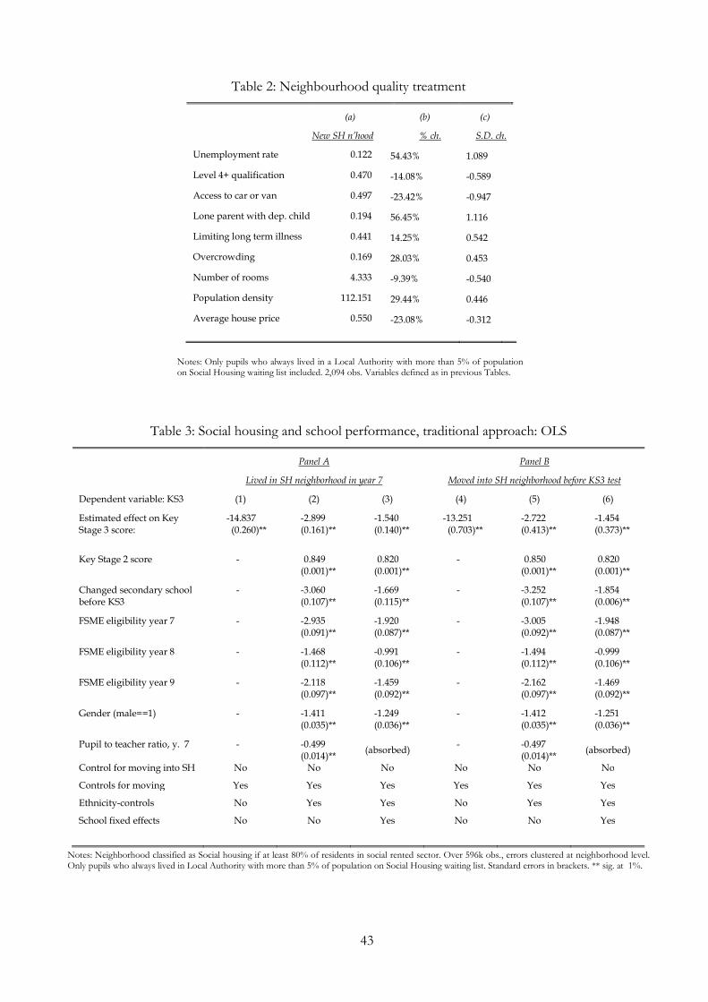
43
Notes: Only pupils who always lived in a Local Authority with more than 5% of population on Social Housing waiting list included. 2,094 obs. Variables defined as in previous Tables.
Table 3: Social housing and school performance, traditional approach: OLS
Panel A
Lived in SH neighborhood in year 7
Panel B
Moved into SH neighborhood before KS3 test
Dependent variable: KS3 (1) (2) (3) (4) (5) (6)
Estimated effect on Key Stage 3 score:
-14.837 (0.260)**
-2.899 (0.161)**
-1.540 (0.140)**
-13.251 (0.703)**
-2.722 (0.413)**
-1.454 (0.373)**
Key Stage 2 score - 0.849 (0.001)**
0.820 (0.001)**
- 0.850 (0.001)**
0.820 (0.001)**
Changed secondary school before KS3
- -3.060 (0.107)**
-1.669 (0.115)**
- -3.252 (0.107)**
-1.854 (0.006)**
FSME eligibility year 7 - -2.935 (0.091)**
-1.920 (0.087)**
- -3.005 (0.092)**
-1.948 (0.087)**
FSME eligibility year 8 - -1.468 (0.112)**
-0.991 (0.106)**
- -1.494 (0.112)**
-0.999 (0.106)**
FSME eligibility year 9 - -2.118 (0.097)**
-1.459 (0.092)**
- -2.162 (0.097)**
-1.469 (0.092)**
Gender (male==1) - -1.411 (0.035)**
-1.249 (0.036)**
- -1.412 (0.035)**
-1.251 (0.036)**
Pupil to teacher ratio, y. 7 - -0.499 (0.014)**
(absorbed) - -0.497
(0.014)** (absorbed)
Control for moving into SH No No No No No No
Controls for moving Yes Yes Yes Yes Yes Yes
Ethnicity-controls No Yes Yes No Yes Yes
School fixed effects No No Yes No No Yes
Notes: Neighborhood classified as Social housing if at least 80% of residents in social rented sector. Over 596k obs., errors clustered at neighborhood level. Only pupils who always lived in Local Authority with more than 5% of population on Social Housing waiting list. Standard errors in brackets. ** sig. at 1%.
Table 2: Neighbourhood quality treatment
(a) (b) (c)
New SH n’hood % ch. S.D. ch.
Unemployment rate 0.122 54.43% 1.089
Level 4+ qualification 0.470 -14.08% -0.589
Access to car or van 0.497 -23.42% -0.947
Lone parent with dep. child 0.194 56.45% 1.116
Limiting long term illness 0.441 14.25% 0.542
Overcrowding 0.169 28.03% 0.453
Number of rooms 4.333 -9.39% -0.540
Population density 112.151 29.44% 0.446
Average house price 0.550 -23.08% -0.312

44
Table 4: Main results: social housing and school performance, the causal effect
(1) (2) (3) (4)
Dependent variable: KS3 test scores
Moved into SH n’hood
Moved into non-SH n’hood
First Difference
DiD
Panel A: Unconditional means
Move before KS3 test 33.598 46.849 -13.251 -0.365
Move after KS3 test 32.962 45.847 -12.886
Panel B: Regression estimates
Move into SH neighborhood before KS3 test -0.365
(1.056)
0.426
(0.628)
0.539
(0.597)
0.267
(0.651)
Move into SH neighborhood before or after KS3 test -12.886
(0.801)**
-3.152
(0.481)**
-2.000
(0.454)**
0.097
(0.515)
Key Stage 2 score - 0.850
(0.001)**
0.820
(0.001)**
0.830
(0.001)**
Changed secondary school before KS3 - -3.251
(0.107)**
-1.854
(0.116)**
-2.763
(0.120)**
FSME eligibility year 7 - -3.001
(0.092)**
-1.946
(0.087)**
-1.439
(0.101)**
FSME eligibility year 8 - -1.494
(0.112)**
-1.466
(0.092)**
-0.924
(0.123)**
FSME eligibility year 9 - -2.156
(0.097)**
-1.466
(0.092)**
-1.058
(0.107)**
Gender (male==1) - -1.412
(0.035)**
-1.251
(0.036)**
-1.525
(0.040)**
Pupil to teacher ratio, year 7 - -0.497
(0.014)**
(absorbed) -0.549
(0.019)**
Control for moving into social housing Yes Yes Yes Yes
Controls for effects of moving Yes Yes Yes Yes
Ethnicity-controls No Yes Yes Yes
School fixed effects No No Yes No
Output Area fixed effects (after move) No No No Yes
Notes: Neighborhoods classified as Social housing if at least 80% of residents in social rented sector. SH movers who move only once. Only pupils who always lived in Local Authority with more than 5% of population on Social Housing waiting list. Over 596k obs., errors clustered at neighborhood level. Standard errors in brackets. ** sig. at 1%.

45
Table 5: Testing for heterogeneity
(1)
(2)
(3)
(4)
Dependent variable: KS3 test scores
Changed School
before KS3
Gender (male=1)
Change in n’hood % unemp’t.
Change in n’hood %
lone parents
Interaction * Move into SH n’hood
before KS3
-1.770
(4.220)
-2.453
(2.128)
0.010
(0.169)
-0.016
(0.097)
Interaction* Move into SH n’hood
before or after KS3
1.368
(3.790)
2.536
(1.620)
0.020
(0.127)
-0.021
(0.074)
Move into SH neighborhood
before KS3
-0.359
(1.10)
0.795
(1.462)
-0.114
(1.269)
0.324
(1.250)
Move into SH neighborhood
before or after KS3
-12.801
(0.816)**
-14.124
(1.085)**
-13.838
(0.980)**
-13.731
(0.926)**
Control for moving into social housing Yes Yes Yes Yes
Controls for effects of moving Yes Yes Yes Yes
Ethnicity-controls No No No No
School fixed effects No No No No
Output Area fixed effects (after move) No No No No
Notes: Baseline regressions is Table 4 (column 1). Interaction main effects and for non-SH movers always included (coefficients not reported here). Neighborhoods classified as social housing if at least 80% of residents in social rented sector. Movers only move once. Only pupils who always lived in Local Authority with more than 5% of population on Social Housing waiting list. Over 596k obs., errors clustered at neighborhood level. Standard errors in brackets. ** sig. at 1%.

46
Table 6: Probability of moving in the two years before versus after the KS3 test
(1) (2) (3)
Moving into SH n’hood
Moving out of SH n’hood
Non-SH n’hood move
Key Stage 2 score -0.0097 (0.044)
-0.0076 (0.039)
0.0173 (0.006)**
FSME eligibility year 7 -0.030 (0.033)
0.015 (0.028)
0.024 (0.006)**
FSME eligibility year 8 0.051 (0.038)
0.009 (0.331)
-0.004 (0.008)
FSME eligibility year 9 0.006 (0.032)
-0.037 (0.029)
-0.016 (0.007)**
Gender (male==1) 0.011 (0.021)
-0.011 (0.018)
0.012 (0.003)**
Ethnicity-White British Isles 0.121 (0.075)
0.046 (0.062)
0.009 (0.009)
Ethnicity-Other White 0.051 (0.093)
-0.024 (0.086)
0.006 (0.014)
Ethnicity-Asian 0.130 (0.080)
0.009 (0.073)
0.021 (0.011)$
Ethnicity-Black 0.121 (0.073)
-0.041 (0.066)
0.006 (0.012)
Ethnicity-Chinese 0.163 (0.127)
-0.134 (0.158)
0.010 (0.030)
Ethnicity-Mixed -0.228 (0.095)
0.074 (0.073)
-0.001 (0.013)
Ethnicity-Other -0.001 (0.006)
-0.080 (0.096)
0.005 (0.018)
Teacher to pupil ratio (y7) -0.001 (0.006)
0.002 (0.006)
-0.002 (0.001)*
Cohort -0.010 (0.022)
-0.026 (0.019)
-0.022 (0.003)**
School FX No No No
H0: All coefficients equal zero. Prob> chi2 0.2996 0.1461 0.000
Notes: Dependent variable equals one if pupil move before KS3 in sample where everyone move once and into Social Housing neighborhoods, hence either before or after KS3. (a): 2,094 obs.; (b): 2,977 obs.; (c): over 105,000 obs. Probit regression, marginal effects. Standard errors in brackets and clustered at neighborhood level. Only pupils who always lived in Local Authority with more than 5 per cent of population on Social Housing waiting list included.

47
Table 7: Balancing regressions by type of move
Dependent Variable:
KS2 test scores
(1) (2) (3) (4)
Moving into SH n’hood, OLS
Non-SH n’hood move, OLS
Moving into SH n’hood
Non-SH n’hood move
Move before KS3 -0.437 (1.082)
0.396 (0.159)*
0.092 (1.053)
0.443 (0.148)**
Move -12.802 (0.824)**
-4.208 (0.126)**
-7.023 (0.809)**
-2.908 (0.117)**
School FX NO NO YES YES
Notes: Neighborhood classified as Social housing if at least 80% of residents in social rented sector. Over 596k obs., errors clustered at neighborhood level. Only pupils who always lived in Local Authority with more than 5% of population on Social Housing waiting list. Standard errors in brackets. ** sig. at 1%, * sig. at 5%.
Table 8: Sample selection
Effect of moving into SH n’hood
Panel A: 20% vs 80% threshold: 0.400
(1.231)
Panel B: Excluding y9-10 movers: -0.532
(0.857)
Panel C: Only first cohort: -0.392
(1.059)
Panel D: Only movers: -0.013
(1.063)
Notes: All regressions include Output Area (neighborhood) fixed effects, like Table 4 (column 4). Standard errors in brackets.

48
Table 9: Expanding the treatment period, years 6-9 and years 9-11 movers
(1) (2) (3) (4)
Move into SH neighborhood before KS3, between
years 6 and 9.
-0.990
(1.348)
0.883
(0.825)
0.864
(0.783)
0.083
(0.992)
Move into SH neighborhood before or after KS3,
between years 6 and 11
-12.767
(1.145)**
-3.596
(0.704)**
-2.344
(0.669)**
-0.177
(0.861)
Control for moving into social housing Yes Yes Yes Yes
Controls for effects of moving Yes Yes Yes Yes
Ethnicity-controls No Yes Yes No
School fixed effects No No Yes No
Output Area fixed effects (after move) No No No No
Notes: Here we compare KS3 scores for pupils who move into social housing neighborhoods during three years prior to taking the KS3 compared to pupils who move during the two years afterwards. Neighborhoods classified as Social housing if at least 80 per cent of residents in social rented sector. Movers only move once. Only pupils who always lived in Local Authority with more than 5% of population on Social Housing waiting list. 280k observations (based on only one cohort), 2,419 schools.
FIGURE 2: THE ENGLISH SCHOOL SYSTEM AND IDENTIFICATION
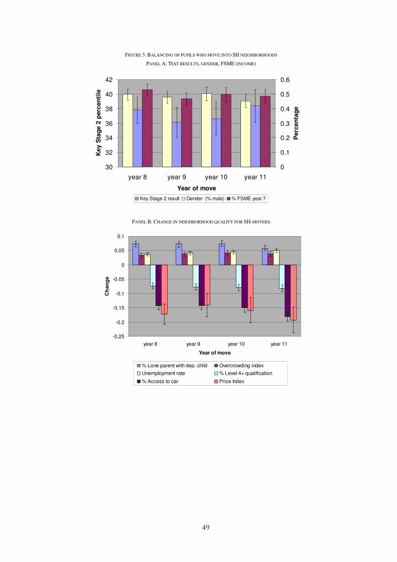
49
FIGURE 3: BALANCING OF PUPILS WHO MOVE INTO SH NEIGHBORHOODS
PANEL A: TEST RESULTS, GENDER, FSME (INCOME)
PANEL B: CHANGE IN NEIGHBORHOOD QUALITY FOR SH-MOVERS
30
32
34
36
38
40
42
year 8 year 9 year 10 year 11
Year of move
Key S
tag
e 2
perc
en
tile
0
0.1
0.2
0.3
0.4
0.5
0.6
Perc
en
tag
e
Key Stage 2 result Gender (% male) % FSME year 7
-0.25
-0.2
-0.15
-0.1
-0.05
0
0.05
0.1
year 8 year 9 year 10 year 11
Year of move
Ch
an
ge
% Lone parent with dep. child Overcrowding index
Unemployment rate % Level 4+ qualification
% Access to car Price Index
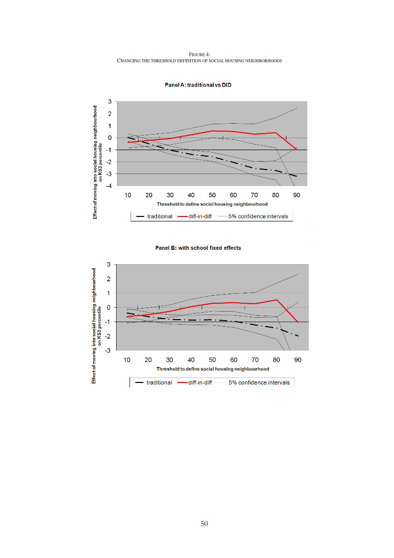
50
FIGURE 4:
CHANGING THE THRESHOLD DEFINITION OF SOCIAL HOUSING NEIGHBORHOODS