NEEP CI Persistence Report-FINAL - MA Energy …ma-eeac.org/wordpress/wp-content/uploads/Lighting...Experience you can trust. Final Report C&I Lighting Measure Life and Persistence

Experience you can trust.

Final Report

C&I Lighting Measure Life and Persistence Project

Prepared for the Regional Evaluation, Measurement & Verification Forum

Middletown, Connecticut June 29, 2011

Experience you can trust.

Copyright © 2011, KEMA, Inc.

The information contained in this document is the exclusive, confidential and proprietary property of

KEMA, Inc. and is protected under the trade secret and copyright laws of the U.S. and other

international laws, treaties and conventions. No part of this work may be disclosed to any third party

or used, reproduced or transmitted in any form or by any means, electronic or mechanical, including

photocopying and recording, or by any information storage or retrieval system, without first receiving

the express written permission of KEMA, Inc. Except as otherwise noted, all trademarks appearing

herein are proprietary to KEMA, Inc.

Table of Contents

KEMA, Inc. June 9, 2011 i

Preface .......................................................................................................................................... 1

1. Executive Summary ............................................................................................................... 2

1.1 Sample Frame Development ........................................................................................ 3

1.2 Site Survey Methodology .............................................................................................. 4

1.3 Survival Analysis Methods ............................................................................................ 5

1.4 Results .......................................................................................................................... 6

1.5 Conclusions and Recommendations ............................................................................ 8

2. Introduction and Study Overview ......................................................................................... 10

3. Methodology ........................................................................................................................ 12

3.1 Sample Frame Development ...................................................................................... 12

3.2 Sample Design ........................................................................................................... 15

3.3 Site Survey Methodology ............................................................................................ 21

3.4 Survival Analysis Methods .......................................................................................... 22

4. Results ................................................................................................................................. 33

4.1 Pre-Modeling Results ................................................................................................. 33

4.2 Survival Analyses Results .......................................................................................... 36

4.2.1 Overall Results by Technology ....................................................................... 44

4.2.2 Results by Large and Small ............................................................................ 45

4.2.3 Results by Building Type ................................................................................ 46

4.2.4 Results by Hours of Use ................................................................................. 47

4.3 Secondary Equipment Life Research ......................................................................... 48

4.4 Equipment Lifetime Hours Comparison ...................................................................... 51

4.5 Secondary and Weibull Model EUL Comparison ....................................................... 52

5. Conclusions and Recommendations ................................................................................... 53

Appendix A: Sample Site Survey Form ....................................................................................... 56

Appendix B: Building Type Categorizations ................................................................................ 59

Appendix C: On-Site Recruitment Protocol ................................................................................. 60

Appendix D: Technical Appendix ................................................................................................ 64

List of Exhibits:

Table 1-1: Phases of Study Approach .......................................................................................... 2

Table 1-2: Sample Design Coverage by Year Category and Measure Type ................................ 3

Table 1-3: Final Sample Compared to Sample Design ................................................................. 4

Table of Contents

KEMA, Inc. June 9, 2011 ii

Table 1-4: EUL Estimates by Technology ..................................................................................... 6

Table 1-5: Summary of all EUL Results at 80% CI ....................................................................... 8

Table 3-1: Preliminary Assessment of Project Data by Program Type, State and Year ............. 13

Table 3-2: Summary of Projects by Technology in Sample Frame ............................................. 14

Table 3-3 Final Proposed Measure Combination Allocation (300 Project Target) ...................... 15

Table 3-4 Preliminary Measure Combination Allocation (300 Project Target) ............................ 16

Table 3-5 Proposed Measure Combination by Year Category Percentages .............................. 17

Table 3-6: Reasons for Sample Replacements .......................................................................... 18

Table 3-7: Final Sample Measure Counts Compared to Sample Design ................................... 19

Table 3-8: Final Sample Counts by Strata .................................................................................. 19

Table 3-9: Population and Sample, Sponsor Percentage of Projects, Savings and Products .... 20

Table 3-10: Final Status of All Recruited Projects ...................................................................... 21

Table 3-11: Proportions of Actual and Representative Products Checked ................................. 22

Table 4-1: Pre-Modeling CFL Bulb Results ................................................................................ 34

Table 4-2: Pre-Modeling CFL Fixture Results ............................................................................. 34

Table 4-3: Pre-Modeling LED Exit Sign Results ......................................................................... 35

Table 4-4: Pre-Modeling HID Results ......................................................................................... 35

Table 4-5: Pre-Modeling T8 Results ........................................................................................... 36

Table 4-6: Non-retention and Failure Event Summary ............................................................... 37

Table 4-7: EUL Estimates by Technology ................................................................................... 45

Table 4-8: Estimated EUL by Program Size and Technology ..................................................... 46

Table 4-9: Estimated EUL by Building Type and Technology ..................................................... 47

Table 4-10: Estimated EUL by Hours of Use and Technology ................................................... 48

Table 4-11: Secondary Source Measure Lifetimes ..................................................................... 51

Table 4-12: Secondary T8 EULs ................................................................................................. 52

Table 5-1: Summary of EUL Results at 80% CI .......................................................................... 54

Table 5-2: Summary of EUL Results at 90% CI .......................................................................... 55

Table 5-3: Design Effect under Different Strategies ................................................................... 89

Table 5-4: Adjusted Model Statistics for Overall Model .............................................................. 91

Table 5-5: Adjusted Model Statistics for Model by Program Size ............................................... 92

Table 5-6: Adjusted Model Statistics for Business Type Model .................................................. 93

Table 5-7: Adjusted Model Statistics for Load Factor Model ...................................................... 94

Table 5-8: Estimated Surviving Proportion by Technology and Time ......................................... 95

Table of Contents

KEMA, Inc. June 9, 2011 iii

Figure 1-1: Weibull EULs vs. Secondary EULs ............................................................................ 7

Figure 2-1: Phases of Study Approach ....................................................................................... 10

Figure 4-1: Estimated EUL for CFL Bulbs ................................................................................... 38

Figure 4-2: Estimated EUL for CFL Fixtures ............................................................................... 39

Figure 4-3: Estimated EUL for HIDs with Outlier ........................................................................ 40

Figure 4-4: Estimated EUL for HIDs without Outlier ................................................................... 41

Figure 4-5: Estimated EUL for HIDs with down-weighted Outlier ............................................... 42

Figure 4-6: Estimated EUL for LED Exits .................................................................................... 43

Figure 4-7: Estimated EUL for T8 Fixtures ................................................................................ 44

Figure 4-8: Weibull EULs vs. Secondary EULs .......................................................................... 52

Figure 5-1: Two Methods of Calculating a Confidence Interval for the EUL ............................... 65

KEMA, Inc. June 29, 2011 1

Preface

The Regional EM&V Forum

The Regional EM&V Forum (Forum) is a project managed and facilitated by Northeast Energy

Efficiency Partnerships, Inc. The Forum’s purpose is to provide a framework for the development

and use of common and/or consistent protocols to measure, verify, track and report energy

efficiency and other demand resource savings, costs and emission impacts to support the role and

credibility of these resources in current and emerging energy and environmental policies and

markets in the Northeast, New York, and Mid-Atlantic region. Jointly sponsored research is

conducted as part of this effort. For more information, see http: www.neep.org/emv-forum.

Acknowledgments

Thomas Ledyard from KEMA managed the project, assisted by many KEMA colleagues, including

Miriam Goldberg, Ken Agnew, Paulo Tanimoto, Jeff Zynda and Aaron Kwiatkowski. Stephen Waite

served as technical advisor to NEEP throughout this project.

Subcommittee for the Commercial Lighting Persistence Project

A special thanks and acknowledgment from Elizabeth Titus on behalf of EM&V Forum staff and

contractors is extended to this project’s subcommittee members and other Forum sponsors from

Maine, New Hampshire, Vermont, Massachusetts, Rhode Island, Connecticut, and New York, many

of whom provided input, including data from a range of lighting programs, during the development

of this project: Bill Blake and Dave Jacobson, National Grid; Judeen Byrne and Victoria Engel-

Fowles, NYSERDA; Mary Cahill , Maribel Cruz-Brown and Josu Omaechevarria, NYPA; Mark

Churchill and Dave Weber, NSTAR; Elizabeth Crabtree, Efficiency Maine; Gene Fry, Northeast

Utilities; Dimple Gandhi, representing Long Island Power Authority; Lisa Glover, Unitil; Paul Gray,

United Illuminating; Paul Horowitz, independent consultant; Nikola Janjic, Efficiency Vermont;

Kathryn Mammen and Bill Saxonis, NY Public Service Commission; Kim Oswald, consultant to

Connecticut Energy Efficiency Board; Mark Sclafani, Central Hudson; Earle Taylor, consultant to

Northeast Utilities; John Zabliski, Rochester Gas and Electric.


1. Executive Summary

The primary objective of this study was to conduct primary and secondary research and analysis to

provide the sponsors with estimates of measure lifetimes that included on-site verification of CFL

bulbs and fixtures, LED exit signs, HID fixtures, and T8 fixtures installed by commercial and

industrial lighting programs in New England and New York. A second objective was to determine

the expected operating lives (in hours) for the same equipment categories; based on secondary

data. A primary driver of this study was the need for lighting measure lives for use in submitting

demand resources into the ISO-NE Forward Capacity Market.

Table 1-1 presents an overview of the study design. The original RFP had sequential tasks that

included primary data collection and the subsequent analyses of that data. In the work plan KEMA

divided the work into four phases and inserted two checkpoints to provide the forum with the

authority to approve and modify the work scope. These checkpoints occurred at the conclusion of

Phase 1 and the conclusion of Phase 2. This phased approach was developed as a mechanism to

deal with potential data availability challenges in the opening study tasks. In this manner, there

were clear opportunities for the study to become dependent on secondary research if insufficient

data was not available to perform primary data collection, but this ended up not being necessary.

Table 1-1: Phases of Study Approach


1.1 Sample Frame Development

The sponsors provided tracking system data for C&I program lighting installations that occurred

from 1999-2009. Using this data, KEMA developed a representative sample of installations from

which primary data collection was gathered and used to determine measure persistence in years of

survival and other statistical modeling analyses.

Due to the fact that projects often had more than one measure type installed through a given

program, measure combination groups were created in order of their weighted probability

(proportion of total estimated savings) in the population. Using these probabilities the measure

goals in Table 1-2 were created for these groups (or strata), which were defined as CFL fixtures

with any other technology, CFL bulbs with or without HIDs or T8s but without CFL fixtures, HIDs

with or without T8s but without CFL fixtures and bulbs, and T8s only.

The sample was designed to ensure coverage of each of the measure goals in Table 1-2 beginning

with CFLF and working to the left. For instance, 23 projects that occurred between 1999 and 2002

(Year Category 1) and consisted of at least CFL fixture installations (according to sponsor tracking

systems) were selected to satisfy the sample size in that cell (CFLF, Year Category 1). If three of

these projects also had CFL bulbs installed, then only 18 more projects which had CFL bulb

installations that occurred from 1999-2002 would need to be pulled to reach our sampling quota in

that cell (CFLB, Year Category 1).

Table 1-2: Sample Design Coverage by Year Category and Measure Type

Year Category

Goals

Projects T8 HID CFLB CFLF

1 (1999-2002) 112 87 45 21 23

2 (2003-2006) 91 71 21 22 23

3 (2007-2009) 49 40 14 15 12

Totals 252 198 80 58 58

Due to better measure coverage per sample point than was initially anticipated and the time

required of the sponsors to repeatedly provide detailed files, the sponsors decided to conclude the

on-site effort short of the initial goal of 252 projects. Table 1-3 shows that even though on-sites

were performed to only 224 projects, the sample design goals were reached for all but a few cells.

The cells for which the goals were not met (shaded) came very close to the initial targets.


Table 1-3: Final Sample Compared to Sample Design

Year Category Projects T8 HID CFLB CFLF Sample Design

1 (1999-2002) 112 87 45 21 23

2 (2003-2006) 91 71 21 22 23

3 (2007-2009) 49 40 14 15 12

Sample Design Totals 252 198 80 58 58 Final Sample

1 (1999-2002) 108 92 49 28 35

2 (2003-2006) 73 66 22 28 34

3 (2007-2009) 43 34 12 15 12

Final Sample Totals 224 192 83 71 81

1.2 Site Survey Methodology

The objective for the site survey task was to develop and execute a recruitment and data collection

protocol to capture and report the data required for successful implementation of the survival

models. The recruitment protocol (found in Appendix C) was designed to reduce non-response

bias by allowing for the exploration of all possible avenues to gain access to the sampled sites. The

on-site data collection form was designed so that information on measure type, quantity, model

details (where available from the sample frame), and location could be prefilled on the form. We

provide an example of an on-site form as Appendix A. The detailed data on what was installed

became the reference point from which the on-site was performed. The site survey was designed

to collect the following levels of data on each unit of equipment identified as installed through the

program.

Status of unit at time of visit. KEMA staff sought to determine if the original measures were

still installed and operating at the time of the on-site visit. This was achieved through visual

inspection (including random ballast checks) combined with site contact input.

End of service for units not present. For all measures that were not installed at the time of

the on-site visit, KEMA staff sought to identify when they were removed from the site contact.

Date ranges were accepted when contacts could not provide the exact year of removal.

Reason for end of service. KEMA auditors also sought to identify the reasons why program

measures were removed. Understanding these reasons allowed for an important distinction

between failure and removal/replacement prior to failure. KEMA also tracked whether


businesses were no longer in operation and if there was a new business in its place or if the

building is vacant.

Nearly 1,000 ballasts were checked during the on-site visits; including 740 T8 ballast checks.

When ballast checks suggested burn out rates1, those estimates were applied to locations with the

same schedule within the facility. That is, if an unchecked fixture was of the same fixture type and

had the same reported annual hours of use as another fixture that was checked in the same facility,

it was considered to be represented by the fixtures that were checked.

1.3 Survival Analysis Methods

A measure’s Effective Useful Life (EUL) is defined as its median retention time; that is, the time at

which half the units of the measure installed during a program year are not retained. Typically, a

retention study is conducted when more than half the units of a measure installed during a program

year are still retained. Therefore, it is necessary to employ statistical methods to estimate the

measure’s EUL. To analyze retention, this study employs a method commonly referred to as

Survival Analysis. The set of techniques referred to as Survival Analysis are widely employed to

analyze data representing a period of time.

Kaplan-Meier Estimator

Combining the non-persistence data from multiple program years requires a way to take into

consideration unknown future events. Put another way, we need a method that can handle data

that is installed at the time of the site visit, but that will experience a removal event at some

unknown point in the future (right censoring). Life-test or Kaplan-Meier (KM) survival curves are a

simple yet powerful way to summarize date-specific and right censored data.

If measures have been installed long enough that more than 50 percent of the measures are no

longer in place, a non-parametric approach such as a KM approach, can offer a characterization of

measure persistence. The limitation to the non-parametric approaches is that they cannot be

projected beyond the limits of the maximum elapsed years. In many cases where estimates of

measure persistence are sought, over 50 percent of the measures are still in the field, thereby

limiting the ability to use KM.

1 Burnout in this study refers to when a fixture has failed or died due to its normal use over time (i.e., it was not removed

before failure).


Parametric Survival Analyses

In order to estimate a measure’s EUL, this study assumes the number of years a unit of the

measure is retained, or the time to non-retention of a unit, follows some general path. Technically,

this path is referred to as a distribution. Therefore, the general method of study is to collect data on

the times to non-retention of units and use those data to estimate the specific path or parameters of

the distribution. The estimated path or parameters of the distribution of the time to non-retention of

a unit of a measure are then used to estimate the measure’s median retention time or EUL.

Given the variety of reasons a unit of a measure may not be retained, the general path the time to

non-retention of a unit follows is unclear. Therefore, this study considers a variety of distributional

assumptions, including Gamma, Weibull, Log-normal, and Log-logistic. These are common

distributional assumptions made when conducting Survival Analysis. The Weibull model was

selected as most appropriate for use to provide final EUL estimates.

1.4 Results

All technology level results are presented in the same manner and include a plot of the data that

shows the predicted measure survival over time. In each plot, the y-axis shows the probability of

survival and the x-axis measures time in years. The EUL is indicated with a horizontal line and is

the time at which half of the units are expected to survive. The vertical line indicates the EUL for

the Weibull model.

Table 1-4 provides a summary of the survival model results by technology. More details on each

result is provided in the body of the report, including how we handled an HID outlier site as well as

plots of the survival models. The error at the 80% confidence interval is provided in the final two

columns of this table. The estimated EULs extend from a low of 5.1 years for CFL bulbs to a high

of nearly 22 years for LED exit signs. T8 fixtures have an estimated EUL of just over 16 years.

Table 1-4: EUL Estimates by Technology

Technology Number of Units

Estimated EUL

80% CI Lower

80% CI Upper

CFL Bulb 7,777 5.1 4.3 6.0

CFL Fixture 4,203 7.0 6.4 7.7

LED Exit 1,955 21.9 12.9 37.0

HID 6,732 9.1 8.3 10.1

T8 Fixtures 84,517 16.2 12.8 20.5


Figure 1-1 compares the secondary research estimates discussed above to the Weibull Model

estimates that were derived from the on-site data. We further include the recent estimates of

lifetime provided by GDS on behalf of NEEP as we understand those assumptions have generally

been accepted by the study sponsors. The CFL bulb and T8 estimates are very comparable with

approximately 1 year of difference between each source for both measures. The secondary CFL

fixture and HID estimates are approximately 5-6 years longer than the Weibull estimates, while the

Weibull estimate for LED exit signs is approximately eight years longer than its secondary

counterpart. The error bars show the upper and lower bounds are the Weibull estimate at the 80%

confidence interval.

Figure 1-1: Weibull EULs vs. Secondary EULs

Table 1-5 presents all EUL results by technology and by various sub samples that were explored

and analyzed. Cells are shaded gray to illustrate statistically different results. We provide a two-

tailed, 80% confidence interval around each result. The use of an 80% confidence interval is

consistent with other studies of this nature, including the Retention Study of Pacific Gas and Electric

companies Industrial Program performed in 2003. We also provide results at the 90% confidence

interval in the body of the report. The top row provides overall EULs by technology, with

subsequent rows presenting EULs by program size, annual hours of use and building type.


Table 1-5: Summary of all EUL Results at 80% CI

Overall (80% CI)

CFL bulbs

CFL Fixtures HID LED Exit

T8 Fixtures

5.1 (4.3-6.0)

7.0 (6.4-7.7)

9.1 (8.3-10.1)

21.9 (12.9-37.0)

16.2 (12.8-20.5)

Program Size

Large (n=92) (80% CI)

6.3 (4.9-8.2)

11.3 (8.6-14.8)

8.7 (7.7-9.8)

20.4 (12.0-34.9)

16.7 (13.0-21.6)

Small (n=132) (80% CI)

4.4 (3.6-5.5)

5.9 (5.3-6.5)

9.6 (8.3-11.2)

25.3 (12.0-53.0)

14.2 (9.8-20.8)

Annual HOU Bin

High HOU (n=166) (80% CI)

6.9 (3.9.12.1)

25.4 (5.9-108.6)

10.2 (8.9-11.7)

N/A 13.6 (10.6-17.3)

Low HOU (n=138) (80% CI)

4.7 (3.7-6.0)

9.5 (7.7-11.8)

12.1 (8.4-17.4)

N/A 22.3 (15.2-32.5)

Building Type

Retail/Wholesale (n=70) (80% CI)

3.2 (2.2-4.5)

5.2 (4.3-6.2)

11.2 (8.6-14.6)

12.0 (6.1-23.4)

11.0 (8.7-13.9)

Services (n=106) (80% CI)

6.5 (5.1-8.1)

7.3 (6.6-8.1)

10.4 (8.6-12.6)

22.4 (12.8-39.1)

19.4 (14.0-26.9)

Other (n=51) (80% CI)

5.6 (3.9-8.2)

14.8 (5.2-42.5)

7.5 (6.6-8.5)

47.6 (8.7-262.0)

28.0 (14.2-54.9)

Note: Annual HOU and Building Type sample sizes may exceed the total sample size of 224. Self-reported annual HOU were gathered by space so sites that had areas of both high and low use will be represented in each bin. With regard to building type, two projects were performed in school districts for which visits to multiple building types were performed (services and other).

1.5 Conclusions and Recommendations

We recommend that the sponsors utilize the overall EULs by technology as provided in the top row

of Table 1-5 above. This includes the use of a CFL bulb lifetime of 5.1 years, CFL fixture lifetime of

7 years, HID of 9.1 years, LED exit signs of 21.9 years and T8 fixtures of 16.2 years. While some

sub sample results are statistically different, we have concerns that despite finding these

differences, the sample sizes they are based on are not as robust as the overall EUL estimates

provided. Given the size of some of the sub sample populations, there is an opportunity for chance

events to drive the observed differences in results as opposed to the results being caused by actual

differences between the sub sample groups. For example, a single remodeled site accounts for

21% of the fixtures removed among small business customers in that sub-sample, which drives

much of the difference between the small CFL fixture measure life result and the overall result. In

addition, it should be noted that the dis-aggregation of some results (such as EUL by hours of use)


are dependent upon self reported hours of operation, upon which a distinction between groups is

made that might not be entirely accurate.

Recently, sponsor programs have included T5 and high performance T8 technologies. While these

were not included in the primary research effort of this study, they were included in the secondary

data research to assess the possibility of transferring the primary EUL results to these technologies.

Indeed, T8 fixture hours and lifetimes as noted in the secondary data are very similar to T5 and high

performance T8 estimates. In our experience, the application and location of high performance T8

fixtures can be expected to be similar to those of standard T8 fixtures. To a lesser extent this is

also true of T5, although a common application for T5 fixtures is to replace HID fixtures which can

have different operating conditions and locations than standard T8 fixtures might have.

We believe the T8 EUL results are transferable to T5 and high performance T8 lighting until a more

definitive measure life study on those specific technologies is performed. We conclude this for two

primary reasons. First, much of the T8 fixture lifetimes in our sample were driven by events in

which fixtures were removed before their natural failure, which we believe would also be the primary

driver of T5 and high performance T8 lifetimes. Second, the similarity between the secondary data

on lifetimes and rated hours between T5, HP T8 and T8 fixtures suggests that to the extent natural

failure events do occur, they would likely impact these technologies the same as that observed in

this study.

Finally, while T5 applications are often in place of HID fixtures, we do not recommend the use of the

HID lifetime estimates for T5 fixtures. This is due to the fact that many HID removal events were

replacements of the HID fixture to a linear fluorescent fixture. This removal cause heavily

influenced the HID measure life calculated in this study and is not expected to occur with the T5

lighting technology.


2. Introduction and Study Overview

The primary objective of this study was to conduct primary and secondary research and analysis to

provide the sponsors with estimates of measure persistence. This research included on-site

verification of CFL bulbs and fixtures, LED exit signs, HID fixtures, and T8 fixtures installed by

commercial and industrial lighting programs in New England and New York. The secondary

objective was to determine the expected operating lives (in hours) for the same equipment

categories; based on secondary data.

Figure 2-1 presents an overview of the study design. The original RFP had sequential tasks that

included primary data collection and the subsequent analyses of that data. In the work plan KEMA

divided the work into four phases and inserted two checkpoints to provide the forum with the

authority to approve and modify the work scope. These checkpoints occurred at the conclusion of

Phase 1 and the conclusion of Phase 2. This phased approach was developed as a mechanism to

deal with potential data availability challenges in the opening study tasks. In this manner, there

were clear opportunities for the study to become dependent on secondary research if insufficient

data was available to perform primary data collection, but this ended up not being necessary.

Figure 2-1: Phases of Study Approach

The remainder of this report presents study methods, findings and recommendations. The next

section of this report, Section 2, describes the participant information gathered from the sponsors

and the sampling that was performed. Section 3 discusses the methods employed to estimate a


measure’s EUL and the standard error of the estimate. The calculation of both the confidence

interval for a measure’s EUL and hypothesis tests about the value of a measure’s EUL are also

discussed in Section 3. Section 4 presents the results for each lighting technology, including both

summaries of the raw field results and the survival analysis results. Section 5 provides study

conclusions and recommendations. Appendix A contains the on-site data collection instrument.

Appendix B provides the mapping of building types into the groupings utilized in the report.


3. Methodology

This section of the report provides the methods used to approach each task of the study. We begin

with a discussion of the sample design followed by our on-site methodology. We conclude this

section with a discussion of the various survival analyses undertaken.

3.1 Sample Frame Development

Early in the study, an important task was to build the most comprehensive possible sample frame

for the primary data collection effort. This included an initial effort to assess the availability of

information upon which the study could rest followed by an effort to gather the specific data needed

to perform the sampling. Recall from the figure above that if the PA information was deemed as not

sufficient at the conclusion of these activities, then the study could be redirected and based upon

secondary research alone.

Table 3-1 below provides a summary of the approximate number of projects from each state that

were provided in this task by the sponsors. This information is presented by program type

(combining C&I new construction and retrofit) and year. They are data that were available

electronically and that minimally included a proxy for lighting size, but ideally included the type of

lighting equipment type installed and quantity. Although some assumptions had to be made and

some gaps in the data had to be informed by other sources, the number of lighting projects and the

longitudinal nature of the available data were clearly sufficient for sampling and primary data

collection.


Table 3-1: Preliminary Assessment of Project Data by Program Type, State and Year

State

Program

Type 1999 2000 2001 2002 2003 2004 2005 2006 2007 2008 2009

Ret / NC* 44 44 44 44 44 44 44 49 36 44 48

Sm. Bus.† 1,271 859 2,167 2,125 620 798 846 1,202 1,666 1,271 1,185

Ret / NC 436 436 436 436 968 950 886 852 715 846 767

Sm. Bus. 1,343 1,872 2,297 2,234 2,217 2,235 2,136 2,046 1,981 1,812 2,064

ME Ret / NC ‐ ‐ ‐ ‐ 256 256 256 256 256 256 256

Ret / NC 19 19 19 249 250 268 304 266 259 177 219

Sm. Bus. 51 51 51 601 613 597 710 720 632 434 498

NY Ret / NC 50 68 160 652 713 418 452 608 543 497 860

Ret / NC 263 263 263 263 402 290 278 237 181 263 188

Sm. Bus. 633 633 633 633 702 532 525 625 724 633 692

VT Ret / NC 0 400 400 400 400 400 400 400 733 733 733

4,110 4,644 6,470 7,637 7,185 6,788 6,837 7,260 7,726 6,966 7,509

* Ret / NC refers to commercial and industrial retrofit and new construction programs

† Sm. Bus. Refers to small business programs.

CT

MA

NH

Total

RI

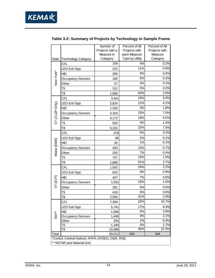
The actual PA data received on lighting projects available from 1999 through 2009 are summarized

in Table 3-2 below. This includes a count of projects for each state. It is important to note that this

table is not a distribution of number of projects, but a count of projects that contain each measure

type; which is why the sum of the utility-level proportions add up to 100%. This look also provides

project counts as a percentage of the total number of projects with that measure across all utilities.

It is easy to see that a higher percentage of projects include T8s than any other measure category

across all but one state.

At the conclusion of gathering and exploring this information, it was decided to focus the study on

four primary technologies. These included HIDs, T8 fixtures, CFL bulbs and CFL fixtures. Although

it was not explicitly focused on in the sampling, it was also agreed that we would gather information

on LED exist signs, which had accumulated significant levels of installations among several

sponsors. While some consideration was made to include T5 fixtures, it was decided that they were

more recently installed measures, so modeling these would not be ideal since there would not be

much evidence of failure.


Table 3-2: Summary of Projects by Technology in Sample Frame

State Technology Category

Number of Projects with a

Measure in Category

Percent of All Projects with each Measure Type by Utility

Percent of All Projects with

Measure Category

CFL 109 4% 0.2%

LED Exit Sign 322 11% 0.5%

HID 266 9% 0.4%

Occupancy Sensors 160 5% 0.2%

Other 57 2% 0.1%

T5 151 5% 0.2%

T8 1,898 64% 2.8%

CFL 3,441 15% 5.0%

LED Exit Sign 2,824 12% 4.1%

HID 1,250 5% 1.8%

Occupancy Sensors 5,163 23% 7.5%

Other 4,172 18% 6.0%

T5 932 4% 1.4%

T8 5,152 22% 7.5%

CFL 218 6% 0.3%


HID 35 1% 0.1%

Occupancy Sensors 493 13% 0.7%

Other 250 7% 0.4%

T5 707 19% 1.0%

T8 1,868 51% 2.7%

CFL 1,542 24% 2.2%


HID 447 7% 0.6%


Other 391 6% 0.6%

T5 418 6% 0.6%

T8 2,030 31% 2.9%

CFL 7,359 22% 10.7%

LED Exit Sign 5,741 17% 8.3%

HID 1,906 6% 2.8%


Other 254 1% 0.4%

T5 1,190 4% 1.7%

T8 15,089 46% 21.9%

Total 69,012 N/A N/A

*ConEd, Central Hudson, NYPA, NYSEG, O&R, RGE

** NSTAR and National Grid

New

Yor

k*

CT

(C

L&P

Onl

y)M

aine

(E

ME

)V

T (

EV

T)

MA

**


3.2 Sample Design

Using the data provided by the sponsors through the data request, KEMA developed a

representative sample of installations from which primary data were gathered and used to

determine measure persistence in terms of the years of survival and other statistical modeling

analyses. The survival model approach puts a premium on model fit, which defined the goal of the

sample design.

Due to the fact that projects often had more than one measure type installed through a given

program, measure combination groups were created in order of their weighted probability

(proportion of total estimated savings) in the population. Using these probabilities the measure

goals in Table 3-3 were created for these groups (or strata), which were defined as follows:

Strata A: CFL fixtures with any other technology

Strata B: CFL bulbs with or without HIDs or T8s but without CFL fixtures

Strata C: HIDs with or without T8s but without CFL fixtures and bulbs

Strata D: T8s only

The sample was originally designed based on a target of 300 total projects. The final allocations,

developed with input from the PAs, included the approximate equalization of the two CFL measures

(combined) with HIDs, with a greater number of projects including only T8s. Table 3-3 summarizes

the overall population from which the sample was developed as well as the proposed targets from

that population. These allocations were based on the expected distribution of specific measures

across the strata which include multiple measure types.

Table 3-3: Final Proposed Measure Combination Allocation (300 Project Target)

Strata (Measure Combination)

Population Sample # Projects in Sample % of

Projects % of

Savings% of

Savings Total CFL

Fixture CFL Bulb HID T8

A CFL Fixture with any other

32% 17% 23% 69 69 8 16 56

B CFL Bulb with or without HID and T8, no CFL fixture

14% 11% 20% 60

60 10 42

C HID with or without T8, no CFLs

10% 15% 37% 111

111 20

D T8 Only 44% 58% 20% 60 60

Totals 100% 100% 100% 300 69 68 137 178


The first two columns show the strata population percentages with respect to number of projects

and savings. The remaining columns summarize the sample given the chosen allocation. The third

column provides the sample percentages with respect to savings. The “Total” column gives the

count of projects in each stratum. The remaining four columns show the expected count of projects

within that stratum that include each fixture type.

The first line illustrates that 69 sample projects from CFL fixture with any other fixture stratum will

be selected. Among those projects we expected 8 projects to have CFL bulbs, 16 projects to have

HID fixtures and 56 projects to have T8 fixtures. Each subsequent line shows the counts of each

measure selected for each stratum. The bottom line shows that a total of 300 were allocated but

that those 300 projects represent 452 project-measure combinations. For any specific sample, the

project-measure combinations will vary. These estimates were based on the average mix of

measures across projects.

Table 3-4 provides the estimated sample pull performed as part of the sample design development.

The strata level allocations were effectively the same2. The number of those allocated projects with

each of the other measures was similar to the expected counts. Though exit lights were not

explicitly included in the sample design, they were included in the analysis based on the project that

had exit light measures.

Table 3-4: Preliminary Measure Combination Allocation (300 Project Target)

Strata (Measure Combination) Projects in Strata

Projects with Measure Type Present

CFL Fixture CFL Bulb HID T8 Exit

A CFL Fixture with any other 70 70 9 16 63 29

B CFL Bulb with or without HID and T8, no CFL fixture

60

60 15 42 28

C HID with or without T8, no CFL 111 111 27 27

D T8 Only 59 59 7

Total 300 70 69 142 191 91

The sample was also distributed across three time periods to force a reasonable distribution across

the 11 years for which project information was available. The percentages in Table 3-5 were

2 The shifting of one project from stratum D to stratum A was an unintended consequence of or rounding error.


applied to the sample size goal of 300 sites to determine the number of projects within each

measure combination/year category we will select. These percentages were used to manage

samples with regards to potential attrition issues.

Table 3-5: Proposed Measure Combination by Year Category Percentages

Strata (Measure Combination)

Time Period

1 (1999-2002) 2 (2003-2006) 3 (2007-2009) Total

A) CFL Fixture with any other 9% 9% 5% 23%

B) CFL Bulb with or without HID and T8, no CFL fixture

8% 8% 4% 20%

C) HID with or without T8, no CFL 15% 15% 7% 37%

D) T8 Only 8% 8% 4% 20%

Total 40% 40% 20% 100%

The final sample produced reflects a number of priorities identified by the sponsors, including a

desire to target results separately for CFL fixtures versus bulbs and the desire for minimum sample

thresholds for each sponsor of the study. We tried to balance these needs amid the primary

challenge of developing a sample design that provides sufficient representation of each measure

group of interest in each installation year bin. In the survival modeling context, defining the sample

in this manner is expected to provide as much quality data as possible to facilitate the most optimal

model fit and resulting precisions.

To ensure that factors such as sample attrition or lack of detailed records would not affect our ability

to perform on-sites, KEMA developed preliminary sample targets based on a sample size goal of

252 sites. The intent was to meet these minimum targets for all measure combination/year

category bins before completing additional sites. KEMA then requested detailed project files for

each project which, at a minimum, needed to include site and customer identification information,

measure type, measure quantity, and measure location to be considered eligible for an on-site visit.

If a particular project file did not contain adequate detail, it was replaced by another project which

consisted of the installation of the same measure type within the same year category (not

necessarily within the same sponsor’s service territory). Throughout the detailed file review and

recruitment processes, 329 projects needed to be replaced for various reasons. As Table 3-6

shows, more than 60% of the replacements were due to a lack of sufficient detail to support an on-

site visit. While a high rate of sample replacement such as this may raise concerns regarding the

potential for selection bias, there is no reason to believe that lighting measure retention at a site is

correlated with the quality or completeness of the program documentation.


Table 3-6: Reasons for Sample Replacements

Reason for Replacement Quantity% of Replacements

(n=329) Lack of sufficient detail

3

198 60.2% Miscategorized measures

4

73 22.2% Sponsor dropped out of study

5

38 11.6% Refused

6

16 4.9% Vacant & inaccessible site

7

4 1.2% Total 329 100.0%

Another finding during the file review process was that some projects included the installation of

more fixture types than the tracking systems initially reported. For instance, a project may have

been selected because it only consisted of T8 installations according to the tracking system, but

the detailed file revealed that CFL bulbs and CFL fixtures were also installed, which gave the

sample more measure coverage per sample point than initially expected.

Due to the increased measure coverage per sample point described above and the time required of

the sponsors to repeatedly provide detailed files, the sponsors decided to conclude the on-site effort

short of the initial goal of 252 projects. Table 3-7 shows that even though on-sites were performed

at only 224 projects, the sample design goals were reached for all but a few cells. The cells for

which the goals were not met (shaded) came very close to the initial targets.

It is important to mention also that 16 projects consisted of installations that occurred at multiple

locations. For these projects, it was decided that we would randomly select up to six locations to

3 Most (85%) of these sites were replaced due to a lack of space-level information, while the remainder were replaced due to a lack of

fixture detail. 4 The large majority (85%) of these instances were of sites that were selected to fulfill an HID sample point according to the tracking

system data that was provided, but the detailed files revealed that no HIDs were actually installed at these sites. The remainder of these

instances consisted of similar situations that occurred with other measure types. 5 Twenty of these were NYPA sites. NYPA decided to drop out of the study on November 8, 2010. The remaining 18 sites were VEIC

sites. While VEIC was able to provide assistance with the initial group of sample points, they were unable to provide assistance with

subsequent samples due to internal resource constraints. 6 One of these sites was a site that VEIC requested not be contacted for an on-site visit because the customer had recently participated

in an on-site evaluation and VEIC did not want to risk upsetting this customer. 7 These four sites were replaced (in accordance with the recruitment protocol) because they were inaccessible and there was no way to

verify if the measures in question were actually still installed. Two other vacant sites were included in the final sample because we were

able to gain access through the property managers to verify that all program measures had been removed.


perform on-site visits (three projects consisted of seven locations so we visited all seven). To

complete visits for 224 projects, we visited a total of 291 locations.

Table 3-7: Final Sample Measure Counts Compared to Sample Design

Year Category Strata D C B A

Projects T8 HID CFLB CFLF Sample Design

1 (1999-2002) 112 87 45 21 23

2 (2003-2006) 91 71 21 22 23

3 (2007-2009) 49 40 14 15 12

Sample Design Totals 252 198 80 58 58 Final Sample

1 (1999-2002) 108 92 49 28 35

2 (2003-2006) 73 66 22 28 34

3 (2007-2009) 43 34 12 15 12

Final Sample Measure Count 224 192 83 71 81 Table 3-8 presents the final sample by strata. Strata A was selected first so 81 sample points were

needed to reach the strata A final measure count shown in Table 3-7 above. Sixteen of the strata A

sites also had CFL bulbs so only 55 more sample points were needed to reach the strata B final

measure count of 71. Thirty-six of the strata A and B sites had HIDs so only 47 more sample points

were needed to reach the strata C final measure count of 83. One-hundred fifty-one strata A, B,

and C sites also had T8s so only 41 more were needed to reach the strata D final measure count of

192.

Table 3-8: Final Sample Counts by Strata

Year Category Total Strata

D C B A

1 (1999-2002) 108 20 30 23 35

2 (2003-2006) 73 10 9 20 34

3 (2007-2009) 43 11 8 12 12

Final Sample Total 224 41 47 55 81

Table 3-9 shows how the final sample compared to the population by number of projects and MWh

savings. Like any sample, this final sample is just one snapshot of the population. There was, in

fact, substantial movement on sponsor counts from sample to sample. The sample percentages by

sponsor are not identical to the population percentages but are generally in line with them. Where


sponsor percentages differ substantially between population and sample, it is primarily because we

allocated to year categories based on set percentages rather than sponsor distributions across the

year categories. In the final completed sample, all sponsors had at least eight sample points, with

the largest quantity coming from NSTAR’s service territory (90). The table also contains the

number of products represented by each sponsor’s sampled sites. As expected, the proportions of

products fall in line with the proportions of projects and savings. The population product counts are

not included as they were not present in all of the sponsors’ tracking data provided for this study.

Table 3-9: Population and Sample, Sponsor Percentage of Projects, Savings and Products

Sponsor

Population Sample

Projects % Savings (MWh) % Projects %

Savings (MWh) %

Product Count %

EME 1,997 5% 32,070 2% 10 4% 1,147 1% 3,383 3%EVT 2,540 7% 103,396 8% 8 4% 2,308 3% 6,688 5%NGR 8,240 22% 85,870 6% 13 6% 778 1% 2,777 2%NSR 14,629 39% 358,354 26% 90 40% 12,260 15% 14,441 12%NU 5,987 16% 122,744 9% 48 21% 5,580 7% 30,740 25%NYSERDA 3,490 9% 634,571 47% 47 21% 56,023 70% 62,787 52%UIL 854 2% 19,067 1% 8 4% 1,936 2% 951 1%Totals 37,737 100% 1,356,072 100% 224 100% 80,032 100% 121,767 100%

The KEMA Team followed a rigorous recruitment protocol that was designed to minimize non-

response bias. If the original business/contact were no longer occupying the site of interest, a new

business/contact was obtained through an internet search and recruited for an on-site visit. If a new

business/contact could not be found on-line, the auditor would drive by the site and attempt to

perform the visit. If the auditor could not complete the visit during a drive-by he/she would gather

information on the new business/contact, which was used to recruit via telephone.

Six of the sampled sites were found to be vacant during the drive-by. Consistent with the

recruitment protocol established at the beginning of this study (see Appendix C), KEMA staff utilized

all of the information available on these six sites so that they could be accessed and included in the

sample. For two of these sites, the auditor was able to gather information on the management

company, which was recruited to gain access to the site to perform the visit, resulting in our ability

to include these vacancies in our analysis. For the remaining four sites, no management company

information was available and the site was replaced, as it was not possible to see if the program

measures were still installed. This rigorous recruiting approach resulted in a replacement rate of

only 6.9%, among sites where recruitment was attempted.


Table 3-10 presents the final status of all 291 projects we attempted to recruit in support of this

study. More than three-quarters (77.0%) became part of the final sample. Sixteen sites refused to

participate in the study (5.5%) and four (1.4%) were vacant and inaccessible. The remaining sites

(16.2%) were still in the recruitment “pipeline” when the on-site effort concluded.

Table 3-10: Final Status of All Recruited Projects

Final Status Quantity% of All Sampled

Projects Completed 224 77.0%

Calling 47 16.2% Refused 16 5.5%

Vacant & Inaccessible 4 1.4% Total 291 100.0%

3.3 Site Survey Methodology

The objective for the site survey task was to develop and execute a data collection protocol to

capture and report the data required for successful implementation of the survival models. The on-

site data collection form was designed so that information on measure type, quantity, model details

(where available from the sample frame), and location could be prefilled on the form. We provide

an example of an on-site form as Appendix A. The detailed data on what was installed became the

reference point from which the on-site was performed. The site survey was designed to collect the

following levels of data on each unit of equipment identified as installed through the program.

Status of unit at time of visit. KEMA staff sought to determine if the original measures were

still installed and potentially operable, even if the space was not in use at the time of the on-site

visit. This was achieved through visual inspection (including random ballast checks) combined

with site contact input. Measures were classified as “installed” if the products listed in the

program tracking system were found to be installed and operating at the time of the on-site visit

and the site contact reported that they were the original products installed through the program.

Measures were classified as “replaced in kind” if the site contact reported that the original

products were replaced with like products.

End of service for units not present. For all measures that were not installed at the time of

the on-site visit, KEMA staff sought to identify when they were removed from the site contact.

Date ranges were accepted when contacts could not provide the exact year of removal.


Reason for end of service. KEMA auditors also sought to identify the reasons why program

measures were removed. Understanding these reasons allowed for an important distinction

between ballast failure and removal/replacement prior to failure. KEMA also tracked whether

businesses were no longer in operation and if there was a new business in its place or if the

building is vacant.

As discussed earlier, ballast checks were performed at the majority of sites visited. To perform a

ballast check, auditors simply opened up randomly selected fixtures and recorded the ballast

manufacturer and model number. A minimum of two fixtures was opened in each selected space.

If the ballast manufacturer and model number of these two fixtures matched one another and the

fixture information (type, wattage, etc.) matched the information in the tracking system, they were

assumed to be the fixtures that were originally installed through the program unless the site contact

reported otherwise. If the ballast manufacturer and model number did not match one another, three

more were opened up in the selected space. Using this information in conjunction with feedback

from the site contact, the auditor determined the proportion of fixtures that were no longer installed.

As Table 3-11 shows, nearly 1,000 ballast checks were performed in total, including 740 T8 fixture

checks. When ballast checks suggested that fixtures had persisted or failed, those estimates were

applied to locations with the same schedule within the same facility. That is, if an unchecked fixture

was of the same fixture type and had the same reported annual hours of use as another fixture that

was checked in the same facility, it was considered to be represented by the fixtures that were

checked. Using this methodology, the ballasts that were checked represented almost 34,000

products.

Table 3-11: Proportions of Actual and Representative Products Checked

Fixture Type

Ballast Checks

Performed

Fixtures Represented by Checks

T8 Fixtures 740 28,331CFL Bulbs 155 4,928CFL Fixtures 45 668

Total 940 33,927

3.4 Survival Analysis Methods

This section of the report discusses the methods employed to estimate measure persistence to

date, each measure’s EUL, the methods employed to estimate the standard error of the estimate,

the calculation of the confidence interval for a measure’s EUL, and hypothesis tests about the value


of a measure’s EUL. A measure’s EUL is defined as its median retention time; that is, the time at

which half the units of the measure installed during a program year are not retained. To analyze

retention, this study employs a method commonly referred to as Survival Analysis. The set of

techniques referred to as Survival Analysis are widely employed to analyze data representing the

duration between observable events. These same approaches were used to disaggregate the

analysis by various sub populations later in this report.

Kaplan-Meier Estimator

Combining the non-persistence data from multiple program years requires a way to take into

consideration unknown future events. Put another way, we need a method that can handle

observations of measures that are installed at the time of the site visit, but that will experience a

removal event at some unknown point in the future (right censoring). Life-test or Kaplan-Meier (KM)

survival curves are a simple yet powerful way to summarize date-specific and right censored data.

These methods produce a non-parametric survival curve that reflects all the available information in

both kinds of data.

If measures have been installed long enough that more than 50 percent of the measures are no

longer in place, a non-parametric approach such as a KM approach, can offer a characterization of

measure persistence. The limitation to the non-parametric approaches is that they cannot be

projected beyond the limits of the maximum elapsed years. In many cases where estimates of

measure persistence are sought, over 50 percent of the measures are still in the field, thereby

limiting the ability to use KM for the EUL estimate. However, the KM approach is still useful for

comparing with the parametric results.

The Kaplan-Meier (KM) estimator is also known as the Product-Limit estimator for reasons that will

become clear shortly. In survival analysis it is common to estimate retention in terms of the survivor

function, which measures the probability that an event time is greater than an arbitrary time. In the

case of the KM estimator, the survivor function at time is given by the cumulative product:

where represent distinct event times; is the number of units retained before

time ; and is the number of units that are not retained at time . For periods prior to , the KM


formula reduces to 1, and for times after , the survivor function is undefined. This is why it is not

possible to produce out-of-sample estimates with the KM estimator.

When the data contains no censoring, the KM estimator possesses an intuitive interpretation: it

corresponds to the proportion of observations with event times greater than (Allison, 1995).

Right-censored data, that is, cases in which the study ended before an event could be observed,

can be handled properly by the KM estimator. However, unlike the parametric models presented in

the next section, the KM estimator cannot handle left- and interval-censored data.

Parametric Survival Analyses

In order to estimate a measure’s EUL, this study assumes the number of years a unit of the

measure is retained, or the time to non-retention of a unit, follows some general path. Technically,

this path is referred to as a distribution. Therefore, the general method of study is to collect data on

the times to non-retention of units and use those data to estimate the specific path or parameters of

the distribution. The estimated path or parameters of the distribution of the time to non-retention of

a unit of a measure are then used to estimate the measure’s median retention time or EUL.

The parameters of the distribution of the time to non-retention of a unit of a measure are estimated

by fitting a general linear regression model to the natural log of the times to non-retention of units

observed in the data. This model can be written as:

jjT )log( ,

where Tj = observed time to non-retention of unit j,

= location parameter or intercept,

= scale parameter, and

j = random error term.

The exponential of the error term of this model (je ) is assumed to follow the standardized form of

the distribution of the time to non-retention of a unit. The general linear regression model is fitted

by maximizing the log-likelihood function for the assumed distribution.

To estimate a measure’s EUL, the estimated parameters of the distribution of the time to non-

retention of a unit of the measure are then employed in the survival function. This function is simply

one minus the cumulative distribution function of the time to non-retention of a unit. The survival

function S(t;) gives the probability of retaining a unit of a measure until at least time t, given the


parameter vector . Therefore, the estimate of a measure’s EUL is the time t* such that the survival

probability S(t*;̂ ) = 0.50, where ̂ is the vector of parameter estimates.


Distribution Options

Given the variety of reasons a unit of a measure may be not retained, the general path the time to

non-retention of a unit follows is unclear. Therefore, this study considers a variety of distributional

assumptions, including Gamma, Weibull, Log-normal, and Log-logistic. These are common

distributional assumptions made when conducting Survival Analysis.

The Gamma distribution is the most general of the distributions listed above. It has three free

parameters, location (), scale (), and shape; whereas the other distributions have only one or two

free parameters. The Gamma distribution includes the Weibull, and Log-normal distributions as

special cases.

The Weibull, Log-normal, and Log-logistic distributions have two free parameters, location and

scale; and the Exponential distribution has one free parameter, location. The Weibull and Log-

normal distributions result as special cases of the Gamma distribution when the shape parameter

equals one and zero, respectively.

The Gamma distribution places fewer constraints on the parameters than the Weibull and Log-

normal distributions. As a result, the parameter estimates obtained assuming the Gamma

distribution will be most based on the data. If one of the other distributions is a good description of

the data, its results will be similar to those of the less constrained Gamma distribution.

Distribution Adopted

To select the most appropriate distribution, we reviewed three things. These are discussed below,

and include implications for the non-retention rate over time; a likelihood ratio test; and maximum of

the log-likelihood function.

Non-Retention Rate Over Time

The distributional assumption has implications for the non-retention rate over time. These

implications are seen via the hazard function h(t;). Roughly, the hazard function can be thought of

as the probability of not retaining a unit of a measure at time t, given the unit has been retained up

to that time. Formally, it is the negative ratio of the survival probability density function dS/dt to the

survival function,

);();(

tS

dtdSth

.


An increasing hazard function means the non-retention rate increases as a unit of a measure ages,

whereas a decreasing hazard function means the non-retention rate decreases as a unit of a

measure ages. If the hazard function is constant, the non-retention rate remains constant as a unit

of a measure ages. The hazard function of the Gamma distribution may have a variety of shapes.

However, it is often difficult to determine which possible shape the hazard function of the Gamma

distribution actually takes on.

The hazard function of the Weibull distribution may have one of three shapes: always decreasing,

always increasing, or constant. If the scale parameter is greater than one then the hazard function

is decreasing, whereas if the scale parameter is less than one then the hazard function is

increasing. If the hazard function of the Weibull distribution is increasing (the scale parameter is

less than one), the rate of increase depends on the value of the scale parameter. If the scale

parameter is between 0.5 and 1, the hazard function is increasing at a decreasing rate; if the scale

parameter equals 0.5, the hazard function is increasing at a constant rate; and if the scale

parameter is between 0 and 0.5, the hazard function is increasing at an increasing rate.

The Log-normal distribution produces a hazard function that increases to a peak then decreases.

The larger the scale parameter, the sooner the hazard function reaches its peak and begins to

decrease. A hazard function that is increasing then decreasing means that for some period of time

after a unit of a measure is installed, the non-retention rate increases as the unit of the measure

ages then, after some point, the non-retention rate decreases as the unit of the measure ages.

The hazard function of the Log-logistic distribution may increase to a peak then decrease or it may

be always decreasing. If the scale parameter is less than one then the hazard function is

increasing then decreasing, whereas if the scale parameter is greater than or equal to one then the

hazard function is always decreasing.

Likelihood Ratio Test

If a distribution is a special case of another distribution, the appropriateness of the former versus

the latter can be formally tested using the likelihood ratio test. Therefore, likelihood ratio tests

comparing the appropriateness of the Weibull, and Log-normal distributions versus the Gamma

distribution were conducted.


Maximum of the Log-Likelihood Function

Recall, under each assumed distribution, the general linear regression model is fitted by maximizing

the log-likelihood function. A larger maximum value of the log-likelihood function suggests a better

model fit.

For CFL bulbs, CFL fixtures, and HIDs, the final choice of distribution was found to make very little

difference to the EUL. The differences observed were well within the confidence intervals. For T8s

and LED Exits, the choice of distribution does make a difference because we only observed a

limited number of non-retained units. In both cases, the optimization procedure did not converge

with the Gamma distribution. We again recommend the results from the Weibull distribution

because it is standard in survival analysis and gave us lower estimates of EUL for T8s and LED

Exits. We chose the Weibull because it is the standard distribution in survival analysis.

Standard Error of a Measure’s EUL Estimate

In order to construct a confidence interval for a measure’s EUL or conduct hypothesis tests about

the value of a measure’s EUL, the standard error of a measure’s EUL estimate is necessary. To

perform this, the general linear regression model is fitted to the log of the times to non-retention of

units of a measure. Therefore, the parameters thus estimated and employed in the survival

function directly produce the log of a measure’s EUL estimate such that the survival probability is

0.50. A measure’s EUL estimate is then obtained by calculating the exponential of this log value

(elog(EUL estimate)). Calculating the standard error of a measure’s EUL estimate, however, is not

as simple because the logarithmic transformation is non-linear.

If the distribution of the log of a measure’s EUL estimate is known, it may be possible to calculate

the exact standard error of the measure’s EUL estimate. However, this distribution is unknown in

this study, as it is in most studies. Therefore, the approximate standard error is calculated by SAS® 8using a first order Taylor expansion of the logarithmic function of the time to non-retention of a unit

of a measure around the measure’s EUL estimate. This approximation is a function of the log of the

measure’s EUL estimate and the standard errors of the parameter estimates of the general linear

regression model.

8 Proc lifereg is used for non-parametric survival analysis. Proc lifetest is the procedure used for the KM

approach.


Adjustment to the Standard Error

When fitting a general linear regression model to the data for a given measure, an observation is

the time to non-retention of a unit of the measure. The calculation of the standard errors of the

parameter estimates assumes each observation is independent. This assumption, however, may

be incorrect when sampling does not occur at the level of a unit of a measure. For example, as is

the case in this study, when sampling occurs at the project level and a project may have obtained a

rebate for more than one unit of a measure. In which case, the times to non-retention of units of a

measure may not be independent because the times to non-retention of units may be more similar

within a project than between projects. However, while the times to non-retention of units of a

measure may be more similar within a project than between projects, they are not expected to be

identical within a project. For example, remodeling, damage, dissatisfaction, or facility closure does

not necessarily lead to the simultaneous removal of all units of a measure installed at a site.

Because the times to non-retention of units of a measure may be more similar within a project than

between projects, the standard errors (of both the log of the measure’s EUL estimate and its EUL

estimate) are adjusted by the square root of the design effect (Kish 1965). If the times to non-

retention of units of a measure are no more similar within a project than between projects, then the

design effect equals one and the unadjusted and adjusted standard errors are equal. Generally,

however, the design effect is greater than one.

The Design Effect

The design effect is used to adjust the standard error of an estimate when the sample that

produced the estimate is not a simple random sample. Initially, as is typical, the standard error of

an estimate of a measure’s EUL is calculated assuming the sample that produced the estimate is a

simple random sample, which it is not. In general, the design effect equals the ratio of the variance

of the sample calculated consistent with the sample design to the variance of the sample calculated

as if it were a simple random sample.


The samples employed in this study are not simple random samples. Rather, the samples

employed in this study are unequal cluster samples. In sampling terminology, a project is a cluster.

The clusters or projects are “unequal” because they contain different numbers of units of a

measure.

While we are interested in the standard error of mean or median time to failure, the design effect is

more easily calculated in the dimension of failure probability. Thus, we calculate the design effect

as:

n

sf

pdeff 2

)1(

)var(

,

where

var(p) = ,

f = n/N, n = number of units in the sample, ny = number of units in the sample in year y, N = number of units in the population, c = number of projects included in the sample, Ai = number of units in project i, pi = proportion of units not retained to date in project i, py(i) = proportion of units not retained in the year of project i, py = proportion of units not retained in year y,

2s = .

This formula can be derived from Kish (1965)9. In this formula, var(p) in the numerator is the

variance of the observed proportion failed at a given time. The observed proportion pi reflects the

random selection of a particular cluster (project) i with its particular underlying survival probability,

and also the random failures of units within that project subject to that probability. Thus, the

observed variability pi –py(i) reflects both the between-cluster variability of cluster-level survival

proportions, and the variability of within-cluster random survival.

9 Kish, Leslie. 1965. Survey sampling. New York: John Wiley & Sons, Inc.


We take the deviations pi –py(i) with respect to the overall proportion py for each year y, rather than

with respect to the overall survival proportion across all units. This within-year variability is used

because the effect of year (time) is accounted for in the model, and we are interested in the design

effect with respect to the remaining variability after time is accounted for. Thus, the numerator is a

pooled estimate of variance, considering each year separately and pooling across years.

The term s2 in the denominator is the variance of a single unit 0/1 observation, given the overall

failure proportion. As for the numerator, this variance is a pooled estimate, pooling across years.

There are other approaches to translating design effect calculations into the survival analysis

context. We have considered a few different approaches. The resulting design effects for different

measures vary by factors up to approximately four, with results for some measures increasing and

others showing a decrease moving from one method to another. The corresponding standard

errors therefore vary by factors up to around two (square root of 4). Thus, the significance tests

should be regarded as indicative, but not definitive. We believe the pooled estimates of design

effects provide reasonable estimates, and the corresponding confidence interval calculations are

useful indicators of the accuracy of the EUL estimates.

Adjusting for Outliers

Statistical analyses can be sensitive to the presence of outliers and survival analysis is no

exception. In particular, one of the sites in the study removed nearly 1,900 HID fixtures before

failure and replaced them with T8 fixtures10

. In contrast, the average number of HID fixtures per site

in the tracking system was about 107. It is natural to expect that this outlier site would have a

strong influence on the results.

There are several strategies for dealing with outliers, ranging from excluding them from the analysis

to including them without any adjustment. In the interest of assessing the sensitivity to the outlier,

we produced results with and without that site. In addition, we also adjusted the results by

assigning the average number of HID fixtures to the outlier and scaling back the number of

replacements. By effectively down-weighting the outlier, the HID results turn out to be, as

expected, between the extremes of including and excluding the site.

10 These T8 fixtures were all installed at the same time approximately 7 years after the original HID fixtures were installed presumably for

energy efficiency reasons. The site contact did not report any technical problems with the original equipment.


In the Technical Appendix (D), we provide details on how we calculated the confidence interval for a

measure’s EUL, including how it is done for the log of a measure’s EUL.


4. Results

This section of the report provides the results of the study. We begin with a discussion of the raw

pre-modeling results we gathered in our observations and site work. We follow this by providing the

results of the survival analyses overall and by sub group. We conclude with the provision and

comparison of our secondary research results to the primary research results.

4.1 Pre-Modeling Results

One of the first steps taken in our analysis was to perform data characterization on each technology

across program years. Plots of percentages of the non-persisting measures for each program year

category provided a useful first step for understanding trends in the data and also provide a basic

comparison and sanity check of the data across program years. These plots allow us to identify

anomalous data. Below we present tables that characterize the information we gathered.

Table 4-1 presents the pre-modeling CFL bulb results by year category from the data gathered on-

site. The proportions that were verified as still installed were relatively similar between year

categories 1 and 2, but saw a large increase in year category 3. Overall, approximately one-third of

the CFL bulbs were still installed across all study years. Almost 40% had failed, while 19% were

removed before failure. The remaining 11% were not found by the auditor and were unknown by

the site contact, were in inaccessible spaces, or were not found and were said to have never been

installed by the site contact.

The overwhelming majority of those removed before failure were caused by upgrades to lower

wattage CFLs than what was installed through the sponsors’ programs (52.7%) or removals due to

remodels (31.0%). It should be noted that the higher proportion of failures in the year category 2 as

compared to year category 1, is due to one site which appeared to replace the 1,628 CFL bulbs

with the same technology (“replaced in kind”) that were installed through a sponsor program 5 years

prior. These “replacements in kind” were identified through conversations with the most

knowledgeable site contact that was available at the time of the visit.


Table 4-1: Pre-Modeling CFL Bulb Results11

Year Category # of

Sites

Tracking System Quantity

% Still Installed

Avg. Annual Hrs of Use

% that

Failed

% Removed

Before Failure

% Don't Know/ Unsure

1 (1999-2002) 28 3,420 32.0% 1,993 26.8% 14.8% 26.4% 2 (2003-2006) 28 9,508 26.4% 3,614 46.2% 22.7% 4.8% 3 (2007-2009) 15 1,577 72.8% 3,356 14.8% 1.7% 10.7%

Total 71 14,505 32.7% 3,179 38.2% 18.6% 10.5%

Table 4-2 shows that nearly 43% of program CFL fixtures were still installed at the time of the on-

site visits. Approximately 39% were removed before they failed mostly due to remodels, but also

due to dissatisfaction and upgrades. Only 3% of program CFL fixture installations were verified to

have failed. It is important to note that the low year category 3 installation proportion (as compared

to that of year category 2) was caused by one site which had removed 478 CFL fixtures during a

remodel.

Table 4-2: Pre-Modeling CFL Fixture Results

Year Category # of

Sites


% Still Installed


% that

Failed

% Removed

Before Failure


1 (1999-2002) 35 2,289 27.9% 3,359 5.8% 56.6% 9.7% 2 (2003-2006) 34 1,892 61.4% 4,788 0.6% 9.5% 28.5% 3 (2007-2009) 12 891 40.0% 6,369 0.0% 53.6% 6.4%

Total 81 5,072 42.5% 4,626 2.8% 38.5% 16.1%

Table 4-3 shows that the majority (86%) of the LED exit signs installed through the program at the

sampled sites are still installed and operating. Approximately 10% were removed before failure;

mostly due to remodels, but also due to upgrades to lower wattage LEDs. None had failed by the

time of the on-site visits. The lower year category 3 percent installed, as compared to year

category 2, was due to one site that had 21 LED exit signs installed in inaccessible areas. These

11 The formula that can be used to calculate a normalized installation rate for any row in any of the pre-modeling tables is: (Tracking

System Quantity – (Tracking System Quantity * % Don’t Know/Unsure)) * % Installed. Likewise, the normalized failure rate for each of

these tables can be calculated using the following formula: (Tracking System Quantity – (Tracking System Quantity * % Don’t

Know/Unsure)) * % that Failed.


inaccessible exit signs are represented in the “% Don’t Know/Unsure” column. All “Don’t

Know/Unsure” counts were not included in the modeled EUL results provided later in this report.

Table 4-3: Pre-Modeling LED Exit Sign Results

Year Category # of

Sites


% Still Installed


% that

Failed

% Removed

Before Failure


1 (1999-2002) 56 1,142 82.4% 8,760 0.0% 13.3% 4.3% 2 (2003-2006) 32 679 91.5% 8,760 0.0% 8.2% 0.3% 3 (2007-2009) 14 219 86.3% 8,760 0.0% 0.0% 13.7%

Total 102 2,040 85.8% 8,760 0.0% 10.2% 4.0%

Table 4-4 presents the pre-modeling HID results. It shows that 61% of the program HID fixtures are

still installed and 35% were removed before failure. Most (86.4%) of those that were removed

before failure were upgraded to more efficient technologies, but some (7.5%) were removed due to

remodels. Only 2% were verified to have failed through the on-site visits. The very low proportion

of installs in year category 2 was caused by one site that had upgraded 1,890 HID fixtures to T8s.

We handled this site uniquely in our survival analyses due to its size and the observed magnitude of

measure removal. This was previously discussed in the survival analysis method section. While

some sites had significant removal events associated for other measure types, the HID outlier

warranted special consideration because it accounts for over 21% of the sampled tracking system

quantity. The other events accounted for no more than 11% of the tracking system quantities

represented in the sample.

Table 4-4: Pre-Modeling HID Results

Year Category # of

Sites


% Still Installed


% that

Failed

% Removed

Before Failure


1 (1999-2002) 49 2,439 53.5% 5,979 6.6% 37.7% 2.2% 2 (2003-2006) 22 2,481 16.9% 4,358 0.8% 80.1% 2.2% 3 (2007-2009) 12 4,026 92.7% 4,736 0.0% 5.4% 1.8%

Total 83 8,946 61.0% 5,004 2.0% 34.9% 2.0%

Table 4-5 shows that 78% of program T8s were still installed at the time of the on-site visits.

Approximately 14% were removed before they failed (mostly due to remodels but also due to

upgrades) and 2% failed. Like the HID results in Table 4-4 few T8 burnouts were observed or

reported in the site work.


Table 4-5: Pre-Modeling T8 Results

Year Category # of

Sites


% Still Installed


% that

Failed

% Removed

Before Failure


1 (1999-2002) 92 36,011 78.1% 4,502 3.8% 11.7% 6.3% 2 (2003-2006) 66 41,144 74.8% 4,286 1.1% 19.9% 4.2% 3 (2007-2009) 34 14,049 86.5% 3,640 0.6% 3.4% 9.5%

Total 192 91,204 77.9% 4,261 2.1% 14.1% 5.8%

4.2 Survival Analyses Results

The primary goal for this study was to produce estimates of measure lives for major measure

groups that reflect the diversity of the included programs and geographies. We performed the core

analysis at the technology level, and then where possible we examined the effect of more specific

characteristics such as hours of operation and building type on measure persistence. All SAS

procedure and Weibull model outputs are provided as a technical appendix (Appendix D) of this

report. In addition, the analysis attempted to disaggregate the drivers of non-persistence,

distinguishing between measure removal and failure.

To do this, we estimated time to failure using a competing risks approach, in which all but failure-

related events are censored in the model. Unfortunately, the results were not consistent with

expectations and were accompanied by large standard errors, undermining our confidence in the

validity of the estimates. The main difficulty in measuring equipment lifetime lies in the fact that we

only observed relatively few cases of failure among the data we collected. On the other hand, we

observed plenty of other non-retention events, including replacements before failure. Table 4-6

presents overall proportions of units for non-retention and failure events. It is important to note that

the “Don’t Know/Unsure” proportions from Table 4-1 through Table 4-5 above have been removed

from the calculation of “Number of Units” provided in the table below. From the table, it is clear that

we do not have sufficient information for producing reliable estimates of equipment lifetime, as none

of the measure types reached a point where at least half of the installed products had failed.


Table 4-6: Non-retention and Failure Event Summary

Technology Number of

Units

Proportion of Non-

Retained Units

Proportion of Units

with Failure Event

CFL Bulb 12,981 63.4% 42.7%

CFL Fixture 4,253 49.3% 3.4%

LED Exit 1,959 10.6% 0.0%

HID 8,764 37.7% 2.1%

T8 85,885 17.2% 2.2%

All technology level results are presented in the same manner and include a plot of the data that

shows the predicted measure survival over time. In each plot, the y-axis shows the probability of

survival and the x-axis measures time in years. The EUL is indicated with a horizontal line and is

the time at which half of the units are expected to survive. The vertical line indicates the EUL for

the Weibull model.

Figure 4-1 below presents the CFL bulb results. The blue line shows the Kaplan-Meier result for

which the 50% survival mark is at approximately 4.3 years. The parametric survival model

produces slightly longer EULs but converge around the Weibull model result of 5.1 years. The

Kaplan-Meier results and survival models are all tightly grouped where the decay crosses the 50%

threshold.


Figure 4-1: Estimated EUL for CFL Bulbs

Figure 4-2 shows that the Kaplan-Meier EUL for CFL fixtures is approximately 7.4 years. The

parametric survival model produces slightly shorter EULs than the Kaplan-Meier result, but

converges around the Weibull model result of 7.0 years.


Figure 4-2: Estimated EUL for CFL Fixtures

The HID results are heavily influenced by one site which had replaced almost 1,900 HID fixtures

with linear fluorescent fixtures before the HID fixtures failed. Due to the fact that this site carries so

much weight, the HID results are presented both with and without it. Figure 4-3 presents the results

with this site included and shows the Kaplan-Meier estimate to be approximately 6.8 years. The

parametric survival model produces longer EULs but converge around the Weibull model result of

7.8 years.


Figure 4-3: Estimated EUL for HIDs with Outlier

Figure 4-4 shows just how much the outlier influences the HID results. Without it HIDs do not reach

the 50% non-retention mark, which is necessary to produce a Kaplan-Meier EUL. The parametric

survival model result jumps from 7.8 years with the outlier to 9.4 years without it.


Figure 4-4: Estimated EUL for HIDs without Outlier

Ultimately KEMA handled the outlier by assigning the average number of HID fixtures to it and

scaling back the number of replacements. Recall, the outlier site had removed nearly 1,900 HID

fixtures before failure and replaced them with linear fluorescent fixtures. In contrast, the average

number of HID fixtures per site in the tracking system was about 107. By effectively down-

weighting the outlier, the HID results turn out to be, as expected, between the extremes of including

and excluding the site. Figure 4-5 shows the HID result after assigning the average weight to the

outlier site. The EUL, estimate resulting from this approach is at 9.1.


Figure 4-5: Estimated EUL for HIDs with down-weighted Outlier

Figure 4-6 presents the LED exit sign results. As was the case in the previous figure, a Kaplan-

Meier EUL cannot be produced because LED exit signs do not reach 50% non-retention. The

parametric survival model produces results that are very different from one another due to the very

low instances of non-retention. Given that the Weibull model provides the lowest EUL among the

survival models, it can be considered a conservative estimate. The Weibull model produces an

estimate of 21.9 years.


Figure 4-6: Estimated EUL for LED Exits

Figure 4-7 shows that T8s also did not experience enough non-retention to produce a Kaplan-Meier

result. While not as different as the LED exit sign results above, the parametric survival model

produces results for T8s that are different from one another due to the very low instances of non-

retention. The Weibull model produces an estimate of 16.2 years.


Figure 4-7: Estimated EUL for T8 Fixtures

4.2.1 Overall Results by Technology

Table 4-7 provides a summary of the survival model results by technology. Note that the HID result

is based upon the use of average weighting for the outlier site. The error at the 80% confidence

interval is provided in the final two columns. The estimated EULs extend from a low of 5.1 years for

CFL bulbs to a high of nearly 22 years for LED exit signs. T8 fixtures have an estimated EUL of just

over 16 years.


Table 4-7: EUL Estimates by Technology

Technology Number

of Products

Estimated EUL

80% CI Lower

80% CI Upper

CFL Bulb 7,777 5.1 4.3 6.0

CFL Fixture 4,203 7.0 6.4 7.7

LED Exit 1,955 21.9 12.9 37.0

HID 6,732 9.1 8.3 10.1

T8 Fixtures 84,517 16.2 12.8 20.5

4.2.2 Results by Large and Small

Table 4-8 presents EUL results by program size and overall for each technology. Program size was

defined as the program type that each sample point participated in. In broad terms, small business

programs during this period primarily had thresholds of monthly demand of less than 200 kW,

although at least one sponsor did use 100 kW as cut off. The Large program size results includes

sample from both retrofit and new construction programs. Of the 92 sample points visits, 67 came

from programs that were retrofit only, 24 came from programs with both retrofit and new

construction eligibility and one came from a New Construction program.

The final column of this table presents the program size coefficient p-value. This value can be used

as an indicator of whether the small and large results are statistically different from one another. If

this value is under 0.20, the small versus large EUL results can be considered statistically different

from the overall result at the 80% confidence interval and can be considered for application

independently. If the p-value is over 0.20, then the small and large results are statistically the same

at the 80% confidence interval. At the 90% confidence interval, the coefficient p-value threshold

used to determine statistical similarity is 0.10. Any value under 0.10 identifies results that are

statistically different and any value over 0.10 identifies results that are statistically the same.


Table 4-8: Estimated EUL by Program Size and Technology

Technology Program

Size Number of Units

Estimated EUL

80% CI Range

90% CI Range

Coefficient p-value

CFL Bulb Overall 7,777 5.1 4.3-6.0 4.1-6.3

Small 4,203 4.4 3.6-5.5 3.4-5.8 0.14

Large 3,574 6.3 4.9-8.2 4.5-8.9

CFL Fixture Overall 4,203 7.0 6.4-7.7 6.2-7.9

Small 2,379 5.9 5.3-6.5 5.2-6.8 0.00

Large 1,824 11.3 8.6-14.8 8.0-16.1

LED Exit Overall 1,955 21.9 12.9-37.0

11.1-43.1

Small 689 25.3 12.0-53.0 9.7-66.2 0.66

Large 1,266 20.4 12.0-34.910.3-40.8

HID Overall 6,732 9.1 8.3-10.1 8.0-10.3

Small 1,268 9.6 8.3-11.2 7.9-11.8 0.48

Large 5,464 8.7 7.7-9.8 7.5-10.2

T8 Fixtures Overall 84,517 16.2 12.8-20.5

12.0-22.0

Small 14,355 14.2 9.8-20.8 8.7-23.3 0.59

Large 70,162 16.7 13.0-21.612.0-23.2

4.2.3 Results by Building Type

At each of the on-sites, KEMA categorized the facility into one of 26 primary building types. of this

report provides the means in which we categorized those 26 primary building type categories into

the three categories in Table 4-9 below. Like Table 4-8 above, if the p-value is lower than 0.20, the

results among the various business types can be considered statistically significant at the 80%

confidence interval. Likewise, a p-value lower than 0.10 signifies that business type results are

statistically different at the 90% confidence interval.


Table 4-9: Estimated EUL by Building Type and Technology

Technology Business Type Number of Units

Estimated EUL

80% CI Range

90% CI Range

Coefficient p-value

CFL Bulb

Overall 7,777 5.1 4.3-6.0 4.1-6.3

Retail/Wholesale 1,317 3.2 2.2-4.5 1.9-5.3

0.03 Services 4,856 6.5 5.1-8.1 4.8-8.7

Other 1,604 5.6 3.9-8.2 3.4-9.5

CFL Fixture

Overall 4,203 7.0 6.4-7.7 6.2-7.9

Retail/Wholesale 654 5.2 4.3-6.2 4.1-6.6

0.05 Services 3,177 7.3 6.6-8.1 6.4-8.3

Other 372 14.85.2-42.5

3.5-63.1

LED Exit

Overall 1,955 21.912.9-37.0

11.1-43.1

Retail/Wholesale 185 12.06.1-23.4

4.9-29.6

0.40 Services 1,506 22.412.8-39.1

10.9-46.0

Other 264 47.68.7-

262.05.0-

456.5

HID

Overall 6,732 9.18.3-10.1

8.0-10.3

Retail/Wholesale 3,734 11.28.6-14.6

7.9-15.8

0.10 Services 1,232 10.48.6-12.6

8.1-13.3

Other 1,766 7.5 6.6-8.5 6.4-8.9

T8

Overall 84,517 16.212.8-20.5

12.0-22.0

Retail/Wholesale 25,371 11.08.7-13.9

8.1-14.8

0.05 Services 45,737 19.414.0-26.9

12.8-29.5

Other 13,409 28.014-2-54.9

11.6-67.1

4.2.4 Results by Hours of Use

At each of the on-sites, KEMA gathered self-reported hours of use of the lighting in each facility

area from the occupants of each building. Although not precise estimates, overall, these self

reported estimates of hours are assumed to be fairly accurate. Table 4-10 presents these results.

There are some instances where higher EULs correspond with higher hours of use, which is


counterintuitive. This is due to many instances in which the removal of measures before burnout

interfered with the expected relationship between hours of use and the estimated EULs for some

measures.

We used the hour distribution midpoint of 3,500 annual hours to distinguish low versus high and

calculated the EUL estimates using the same statistical approaches discussed previously. We

consider all results split by hours of use to be statistically the same at both the 80% and 90%

confidence intervals, with the exception of T8 fixtures, which have a P-value of 0.07 and are

therefore statistically different at the 80% and 90% confidence intervals.

Table 4-10: Estimated EUL by Hours of Use and Technology

Technology Load

Factor Number of Units

Estimated EUL

80% CI Range

90% CI Range

Coefficient p-value

CFL Bulb Overall 7,777 5.1 4.3-6.0 4.1-6.3

Low 5,047 4.7 3.7-6.0 3.5-6.4 0.39

High 2,089 6.9 3.9-12.1 3.2-14.8

CFL Fixture

Overall 4,203 7.0 6.4-7.7 6.2-7.9

Low 1,589 9.5 7.7-11.8 7.2-12.6 0.35

High 982 25.4 5.9-108.63.8-

170.5

HID Overall 6,732 9.1 8.3-10.1 8.0-10.3

Low 490 12.1 8.4-17.4 7.4-19.8 0.53

High 5,553 10.2 8.9-11.7 8.5-12.2

T8 Overall 84,517 16.2 12.8-20.5

12.0-22.0

Low 42,925 22.3 15.2-32.513.7-36.3 0.07

High 40,089 13.6 10.6-17.3 9.9-18.6

4.3 Secondary Equipment Life Research

KEMA performed research to compile information on rated hours of operation, annual hours of

operation, and other characteristics related to measure life for many lighting measure types,

including those in this study. The following secondary sources were used:


Source 1: California Database for Energy Efficiency Resources (DEER)12

.

Source 2: Efficiency Vermont Technical Reference User Manual No. 2005-37, dated February

13, 200613

.

Source 3: Efficiency Maine Commercial Technical Reference Manual No. 2006-1, dated March

5, 200714

.

Source 4: CL&P & UI Program Savings Documentation for the 2011 Program Year, dated

September 21, 201015

.

Source 5: Mid-Atlantic Technical Reference Manual, dated October 201016

.

Source 6: Massachusetts Technical Reference Manual, dated October 201017

.

Source 7: New England SPWG Residential & C/I Lighting and HVAC Measure Life Report,

dated June 200718

.

Source 8: Lessons Learned and Next Steps in Energy Efficiency Measurement and Attribution:

Energy Savings, Net to Gross, Non-Energy Benefits, and Persistence of Energy Efficiency

Behavior, dated November 200919

.

Source 9: San Diego Gas & Electric 1996-97 Commercial Energy Efficiency Incentives Ninth

Year Retention Study, dated March 200620

.

Source 10: Southern California Edison Energy Efficiency Incentives Ninth Year Retention

Study, dated February 28, 200621

.

Source 11: Pacific Gas & Electric Energy Efficiency Incentives Ninth Year Retention Study,

dated January 25, 200622

.

Source 12: Technical Reference Manual for Pennsylvania Act 129 Energy Efficiency and

Conservation Program, dated June 201023

.

Sources 13-17: General Electric T8 and Compact Fluorescent Bulb Sell Sheets24

.

12 http://www.deeresources.com/deer0911planning/downloads/EUL_Summary_10-1-08.xls. 13 http://www.state.vt.us/psb/eeurfp2005/trmusermanualno2004-31.doc#_Toc93807418. 14 http://www.cee1.org/eval/db_pdf/565.pdf. 15 http://neep.org/uploads/EMV%20Forum/EMV%20Studies/FINAL%202011%20CT%20PSD.pdf. 16 http://neep.org/uploads/EMV%20Forum/EMV%20Products/Mid%20Atlantic%20TRM_V1.1.pdf. 17 http://www.ma-eeac.org/docs/MA%20TRM_2011%20PLAN%20VERSION.PDF. 18 http://neep.org/uploads/EMV%20Forum/EMV%20Studies/measure_life_GDS%5B1%5D.pdf. 19 http://www.calmac.org/publications/Energy_Efficiency_Measurement_and_Attribution.pdf. 20 http://www.calmac.org/publications/2006_PY96&PY97_CEEI_9th_Year_Retention_Evaluation.pdf. 21 http://www.calmac.org/publications/SCE_9th_Year_Retention_Study_for_96-97_Commercial_Measures,_Final_Report.doc. 22 http://www.calmac.org/publications/PGE_CI_Retention_Final.pdf. 23 http://www.puc.state.pa.us/electric/docs/Act129/Act129_TRM-2010.doc.


Source 18: US Department of Energy (DOE) Energy Efficiency and Renewable Energy

(EERE)25

.

Sources 19 and 20: ENERGY STAR qualifying CFL bulb and fixture lists26

.

Some of the sources listed above provided measure life estimates in years and some provided

these estimates in hours, but none of the sources provided both. Six of the sources provided

annual hours of use estimates by building type, but not by measure type.

Table 4-11 presents the number of sources, range, and average measure life estimates that were

compiled through this secondary research task in both years and hours. Estimates in years were

informed by a review of TRM and PSD documents. Based upon these sources, CFL bulb lifetimes

averaged 4.6 years, CFL fixtures averaged 13.1, LED exit signs and HIDs averaged 14.0, and T8s

averaged 14.7. Within these estimates are those from the GDS study which we understand to be

the primary assumptions being used by many sponsors. The GDS study results provide a CFL bulb

lifetime of 5 years and a lifetime of 13 years for CFL fixtures, LED exit signs, HIDs, and T8s.

The table also provides similar estimates for high performance T8s (HP T8s) and T5s, which are

more efficient options for T8s and HIDs. For both HP T8s and T5s, the average lifetime estimates

in years from the secondary sources are very close to those of the less efficient alternatives. The

rated hours estimates for these technologies are also very similar to that of T8s, although we were

only able to find one source for T5 and HP T8 hours.

The rated hours estimates provided in Table 4-11 are exclusively from manufacturer data, the DOE,

and the ENERGY STAR web site. Except for CFL bulbs, they are the rated hours for ballasts and

not lamps. As such, they represent hours of continuous operation until unit failure, not including

events such as removal, whereas the estimates in years reflect annual hours of operation and, in

some cases, may reflect removal before failure. The average rated hours from these sources was

24http://www.gelighting.com/na/business_lighting/education_resources/literature_library/sell_sheets/downloads/fluorescent/F32T8_SXL-

SPX-ECO_Sell_sheet_74901.pdf, http://www.gelighting.com/na/business_lighting/education_resources/literature_library/sell_

sheets/downloads/fluorescent/F28T8-XL_sell_sheet.pdf, http://www.gelighting.com/na/business_lighting/education_resources

/literature_library/sell_sheets/downloads/fluorescent/LFL-F96T8-49W-SPX-63561.pdf, http://www.gelighting.com/na/business_

lighting/education_resources/literature_library/sell_sheets/downloads/fluorescent/2-3Ft-T8_wm_sell_sheet.pdf,

http://www.gelighting.com/na/business_lighting/education_resources/literature_library/sell_sheets/downloads/cfl/20563_cfl.pdf. 25 http://www1.eere.energy.gov/buildings/ssl/life_measuring.html. 26 http://www.energystar.gov/index.cfm?fuseaction=cfls.display_products_excel, http://downloads.energystar.gov/bi/qplist/fixtures_

prod_list.xls.


9,437 hours for CFL bulbs, 9,800 hours for CFL fixtures, 13,750 hours for HIDs, and 27,333 hours

for T8s.

Table 4-11: Secondary Source Measure Lifetimes

Measure

Estimates in Years (TRMs) Estimates in Rated Hours # of

Sources Range Avg.# of

Sources Range Avg.

CFL Bulbs 8 3.4 to 10 4.6 3 6,000 to 15,000 9,437

CFL Fixt. 9 9.2 to 16 13.1 2 4,000 to 40,000 9,800

HIDs 8 13 to 15 14.0 1 7,500 to 20,000 13,750

HP T8s 7 13-15 13.6 1 N/A 25,000

LED Exits 7 10 to 20 14.0 0 - -

T5s 8 11-16 13.8 1 N/A 25,000

T8s 11 11.2 to 20 14.7 5 18,000 to 40,000 27,333

4.4 Equipment Lifetime Hours Comparison

KEMA attempted to isolate technology failures from other removal events such as remodel or

upgrades. We attempted this analysis in the interest of developing an independent estimate of

rated hours of use that could be cleanly compared to industry-rated equipment life statistics.

Unfortunately, we were not able to disaggregate the lifetimes based solely on unit failure as the

confidence bands were too large around the final failure-only EUL estimates.

To perform an alternate comparison of lifetime hour results to secondary industry data, Table 4-12

presents calculated lifetime hours of each technology based on data gathered from TRMs and the

primary data collected in this study. The secondary side of the table provides the assumed average

hours of use as provided for lighting in the TRMs reviewed along with the TRM EUL estimates. The

right side provides the EUL and self reported operating hours from the on-sites performed in this

study. The calculated lifetime hours are the product of the annual hours of use and the EUL. While

CFL bulb lifetime hour estimates are consistent between the two estimates, CFL and HID fixtures

have notably lower lifetime hours in the current study than in the secondary data, although all of on-

site hours are self reported. LED exits and T8 fixtures have considerably more hours in the current

study than in the secondary data. Despite the fact that these hours are derived from both failure

and non-failure removal events, all technologies have lifetime hours that exceed the average

industry-rated equipment life statistics, which may be due to the self reporting of hours of use from

the on-sites.


Table 4-12: Secondary T8 EULs

Secondary On-site

Technology

# of

Sources

EUL (in

Yrs.) Assumed

AOH

Calculated Equipment

Lifetimes (in Hrs.)

EUL (in

Yrs.) Reported

AOH

Calculated Equipment

Lifetimes (in Hrs.) CFL Bulbs 8 4.6 4,008 18,437 5.1 3,179 16,213

CFL Fixtures 9 13.1 4,008 52,505 7.0 4,626 32,382 HID 8 14.0 4,008 56,112 9.1 5,004 45,536

LED Exits 7 14.0 8,760 122,640 21.9 8,760 191,844 T8 Fixtures 11 14.7 4,008 58,918 16.2 4,261 69,028

4.5 Secondary and Weibull Model EUL Comparison

Figure 4-8 compares the secondary research estimates discussed above to the Weibull Model

estimates that were derived from the on-site data. We further include the recent estimates of

lifetime provided by GDS on behalf of NEEP as we understand those assumptions have generally

been accepted by the study sponsors. The CFL bulb and T8 estimates are very comparable with

approximately 1 year of difference between each source for both measures. The secondary CFL

fixture and HID estimates are approximately 5-6 years longer than the Weibull estimates, and

appear to be statistically different. The Weibull estimate for LED exit signs is approximately 8 years

longer than its secondary counterpart. The error bars show the upper and lower bounds around the

Weibull estimate at the 80% confidence interval.

Figure 4-8: Weibull EULs vs. Secondary EULs


5. Conclusions and Recommendations

Table 5-1 presents all EUL results by technology and by various sub samples. Cells are shaded

gray to illustrate statistically different results. We provide a two-tailed, 80% confidence interval

around each result. The top row provides overall EULs by technology, with subsequent rows

presenting EULs by program size, annual hours of use and building type.

We recommend that the sponsors utilize the overall EULs by technology. While some sub

sample results are statistically different from one another, we have concerns that despite finding

these differences, the sample sizes they are based on are not as robust as the overall EUL

estimates provided. Given the size of some of the sub samples, there is an opportunity for

chance events to drive the observed differences in results as opposed to the results being

caused by actual differences between the sub sample groups. For example, a single remodeled

site accounts for 21% of the fixtures removed among small business customers in that sub-

sample, which drives much of the difference between the small CFL fixture measure life result

and the overall result. In addition, it should be noted that the dis-aggregation of some results

(such as EUL by hours of use) are dependent upon self reported hours of operation, upon which

a distinction between groups is made that might not be entirely accurate.

Recently, sponsor programs have included T5 and high performance T8 technologies. While

these were not included in the primary research effort of this study, they were included in the

secondary data research to assess the possibility of transferring the primary results to these

technologies. Indeed, T8 hours and lifetimes as noted in the secondary data are very similar to

T5 and high performance T8 estimates. In our experience, the application and location of high

performance T8 fixtures can be expected to be similar to those of standard T8 fixtures. To a

lesser extent this is also true of T5, although a common application for T5 fixtures is to replace

HID fixtures which can have different operating conditions and locations than standard T8

fixtures might have.

We believe the T8 EUL results are transferable to T5 and high performance T8 lighting until a

more definitive measure life study on those specific technologies is performed. We conclude

this for two primary reasons. First, much of the T8 fixture lifetimes in our sample were driven by

events in which fixtures were removed before their natural failure, which we believe would also

be the primary driver of T5 and high performance T8 lifetimes. Second, the similarity between

the secondary data on lifetimes and rated hours between T5, HP T8 and T8 fixtures suggests

that to the extent natural failure events do occur, they would likely impact these technologies the

same as that observed in this study.


Finally, while T5 applications are often in place of HID fixtures, we do not recommend the use of

the HID lifetime estimates for T5 fixtures. This is due to the fact that many HID removal events

were replacements of the HID fixture to a linear fluorescent fixture. This removal cause heavily

influenced the HID measure life calculated in this study and is not expected to occur with the T5

lighting technology.

Table 5-1: Summary of EUL Results at 80% CI

Overall (80% CI)

CFL bulbs


T8 Fixtures

5.1 (4.3-6.0)

7.0 (6.4-7.7)

9.1 (8.3-10.1)

21.9 (12.9-37.0)

16.2 (12.8-20.5)

Program Size

Large (n=92) (80% CI)

6.3 (4.9-8.2)

11.3 (8.6-14.8)

8.7 (7.7-9.8)

20.4 (12.0-34.9)

16.7 (13.0-21.6)

Small (n=132) (80% CI)

4.4 (3.6-5.5)

5.9 (5.3-6.5)

9.6 (8.3-11.2)

25.3 (12.0-53.0)

14.2 (9.8-20.8)

Annual HOU Bin


6.9 (397-12.1)

25.4 (5.9-108.6)

10.2 (8.9-11.7)

N/A 13.6 (10.6-17.3)

Low HOU (n=138) (80% CI)

4.7 (3.7-6.0)

9.5 (7.7-11.8)

12.1 (8.4-17.4)

N/A 22.3 (15.2-32.5)

Building Type


3.2 (2.2-4.5)

5.2 (4.3-6.2)

11.2 (8.6-14.6)

12.0 (6.1-23.4)

11.0 (8.7-13.9)


6.5 (5.1-8.1)

7.3 (6.6-8.1)

10.4 (8.6-12.6)

22.4 (12.8-39.1)

19.4 (14.0-26.9)

Other (n=51) (80% CI)

5.6 (3.9-8.2)

14.8 (5.2-42.5)

7.5 (6.6-8.5)

47.6 (8.7-262.0)

28.0 (14.2-54.9)


Table 5-2 presents EUL results by technology and by various sub samples and includes a two-

tailed, 90% confidence interval around each result. Like the previous table, the top row provides

overall EULs by technology, with subsequent rows presenting EULS by program size, annual

hours of use and building type. Cells are shaded gray to illustrate statistically different results.

While CFL bulb results by program size and LED exit results by building type were statistically

different in the table above at the 80% confidence interval, they are not at the 90% confidence

interval.


Table 5-2: Summary of EUL Results at 90% CI

Overall (90% CI)

CFL bulbs


T8 Fixtures

5.1 (4.1-6.3)

7.0 (6.2-7.9)

9.1 (8.0-10.3)

21.9 (11.1-43.1)

16.2 (12.0-22.0)

Program Size

Large (n=92) (90% CI)

6.3 (4.5-8.9)

11.3 (8.0-16.1)

8.7 (7.5-10.2)

20.4 (10.3-40.8)

16.7 (12.0-23.2)

Small (n=132) (90% CI)

4.4 (3.4-5.8)

5.9 (5.2-6.8)

9.6 (7.9-11.8)

25.3 (9.7-66.2)

14.2 (8.7-23.3)

Annual HOU Bin


6.9 (3.2-14.8)

25.4 (3.8-170.5)

10.2 (8.5-12.2)

N/A 13.6 (9.9-18.6)

Low HOU (n=138) (90% CI)

4.7 (3.5-6.4)

9.5 (7.2-12.6)

12.1 (7.4-19.8)

N/A 22.3 (13.7-36.3)

Building Type


3.2 (1.9-5.3)

5.2 (4.1-6.6)

11.2 (7.9-15.8)

12.0 (4.9-29.6)

11.0 (8.1-14.8)


6.5 (4.8-8.7)

7.3 (6.4-8.3)

10.4 (8.1-13.3)

22.4 (10.9-46.0)

19.4 (12.8-29.5)

Other (n=51) (90% CI)

5.6 (3.4-9.5)

14.8 (3.5-63.1)

7.5 (6.4-8.9)

47.6 (5.0-456.5)

28.0 (11.6-67.1)



Appendix A: Sample Site Survey Form

This appendix presents the core site survey form. Note that the area shaded in gray was

merged onto the form before each site visit. We have placed example information into the form

to illustrate this. The auditor used the forms during the walkthrough at each site.

1. Track Fixt Type: The fixture type information from the tracking system.

2. Track Location: The location from the tracking system.

3. Track Qty: The quantity from the tracking system.

4. Onsite Space Type: The location of the fixtures as noted by the auditor during the on-site.

5. Onsite Total: Total fixtures accounted for on-site; includes those installed and those

accounted for by the not found event codes.

6. Onsite Installed: Total fixtures that were installed and operating at the time of the on-site

visit.

7. App. Ann. Hrs.: Estimate of annual hours as estimated by the on-site contact.

8. # Occ. Sensor (OS): Auditor noted the quantity of fixtures that are controlled by occupancy

sensors.

9. OS Setting (Man./Auto): Auditor noted if occupancy sensor(s) are on manual or automatic

setting.

10. OS Loc. (Good/Poor): Auditor noted if the occupancy sensor(s) are installed in good or poor

locations.

11. Removal Event Code: Used to designate why fixture was removed; using the codes below

the table.

12. Removal Event Qty: The quantity removed due to the corresponding removal event.

13. Removal Event Year/Range: The year the removal event occurred in or a range of years if

specific year is not offered. Also indicated if the respondent knew it was removed by a

particular year or was installed through a particular year but could not provide a range or

specific year. For instance, if the contact knew that the fixtures were there in 2004 but could

not say for sure if they were there any later than that, it was written by the auditor as

‘L2004’. If the contact only knew that the fixtures were no longer installed in 2006, but could

not say for sure if they were removed earlier than that, it was written by the auditor as

‘E2006’.

KEMA, Inc. June 9, 2011

57

Example On-Site Form

Pre-Filled Prior to On-Site Visit Auditor Input On-Site Customer Inquiry On-Site

Track Fixture Type Track Location Track Qty

Onsite Space Type

Onsite Total

Onsite Installed

App. Ann. Hrs.

# Occ. Sensor

(OS)

OS Setting (Man./ Auto)

OS Loc. (Good/ Poor)

Not Found Event 1 Not Found Event 2

Code* Qty Year/

Range Code* Qty Year/

Range Fluorescent, (4) 48”, T-8 lamp Main Sales Area 410 Sales 410 410 5,824 0 Fluorescent, (4) 48”, T-8 lamp Bakery Prep By Circle 5 Bakery Prep 5 5 8,760 0 Fluorescent, (4) 48”, T-8 lamp Bakery Circle 6 Bakery Circle 6 6 8,760 0 Fluorescent, (4) 48”, T-8 lamp Frozen Aisles 25 Frozen Aisles 25 25 5,824 0 Fluorescent, (4) 48”, T-8 lamp Main Stockroom 72 Main Stock 72 0 R 72 2005

Fluorescent, (4) 48”, T-8 lamp Customer Service/Entry

32 Customer Svc/Entry

32 26 8,760 6 Auto Good RIK 2 2007 RIK 4 2009

Fluorescent, (4) 48”, T-8 lamp Produce Grid 28 Produce 28 28 8,760 0

Fluorescent, (4) 48”, T-8 lamp Deli, Cheese, Bakery 122 Deli, Cheese,

Bakery 122 122 5,824 0

* Not Found Event Codes: F = Equipment failure, D = Dissatisfied, R = Remodel, V = Location vacant/demolished, C = Change in use of space, U = Equipment upgraded, RIK= Replaced in Kind, T = Temporarily taken out of operation (indicate estimated reinstall date), N = Location not found & unknown by site contact, IEC = Inaccessible and estimated by site contact, IEA = Inaccessible and estimated by the auditor, I = Inaccessible and not able to be estimated, U = Upgraded to a higher efficiency measure (record what this upgraded measure is), NI = Never Installed according to contact, X = Don’t know/Unsure, O = Other (specify). If inaccessible, auditor will try to get fixture type and quantity estimates for the inaccessible space from the site contact or estimate them based on other similar areas in the facility that are accessible.


In addition to visual inspection and customer reports, auditors opened up randomly selected fixtures

to record the manufacturer and model numbers of T8s fixtures, CFL bulbs, CFL fixtures, and HID

fixtures to inform the persistence assessment. When specific conditions were met, auditors

checked two ballasts in the fixture type/space type combinations that had the largest quantity of

program installations (so that the products checked would represent a large proportion of those

installed). If these two ballast model numbers did not match up, the auditor checked additional

ballasts until they could discern an approximate removal rate. Conditions under which ballast

inspections were not performed included the following:

When the customer would not allow the auditor to check the ballasts,

When fixtures were deemed to be unsafe to open due to condition (very old fixtures,

hazardous inspection conditions, unsafe wiring conditions, fixtures that are determined to be

difficult to put back together correctly, ballast covers with screws intended for one use or

that are damaged, fixtures that are dirty and might cause dust to become airborne, etc.),

When fixtures locations did not lend themselves to inspection (such as areas of privacy or

locations where it would otherwise disrupt business).

When fixtures were more than 10 feet off the ground.


Appendix B: Building Type Categorizations

This appendix shows how each of the 26 building types (as agreed upon by the sponsors prior to

the study) were categorized into the three groups presented throughout this report.

Building Type Categorizations

Other

Heavy Industrial Industrial

Refrigeration Light Industrial Multifamily High

Rise Multifamily Low

Rise Other Warehouse

Retail/Wholesale

Big Box Fast Food Full Service Restaurant Grocery

Multi-Story Retail Small Retail

Services

Assembly Auto Repair Community College Dormitory

Hospital Hotel Large Office Motel

Primary School Religious Secondary School Small Office

University


Appendix C: On-Site Recruitment Protocol

Northeast Energy Efficiency Partnership

C&I Lighting Persistence Recruitment Protocol

This document provides a protocol for the recruitment of the site visit work. The objective of this

protocol is to contact sampled sites in a manner that either informs the persistence analysis via

information from the recruitment contact itself or guides the future collection of information via an

on-site or drive-by effort. At the recruitment stage, this means that we employ a system that

rigorously tracks the outcome of the effort to particular final dispositions that lead to either further

known action items or can be used as inputs to the survival analysis itself.

Recruitment Script

If contact name available

Good morning/afternoon. My name is____. I am calling on behalf of <program administrator/retail

affiliate name>. May I speak with <contact name>?

According to our records, your company participated in an energy conservation program with

<utility/retail affiliate name> in <installation year>. Through your participation, <qty> lighting

products were installed at <location>. We are currently performing an assessment of these lighting

products so I was wondering if it be possible for us to schedule a visit to your facility to observe the

installed lighting?


If contact not available from file or if new contact needs to be established:

ON-SITE RECRUITMENT

Yes Schedule a date and time for a visit. Note final disposition as “Appointment scheduled”

below.

Date: ____________ Time: ________ Contact: _____________________

No Can I ask you four quick questions regarding these lighting installations?

1. Since they were installed in <installation year>, have any of these products failed?”

___Yes

___No/Do not Know GOTO ON-SITE RECRUITMENT

2. Approximately what percent of the original quantity are no longer in operation? _____%

3. What type of lighting was installed in their place and what proportion of the products removed were replaced by each? a. ____________________________________ - _____% b. ____________________________________ - _____% c. ____________________________________ - _____%

4. Approximately how many years after installation were they removed and why were they removed*? ______

*If respondent provides removal rates by year, please note specific percentages by

year:

% of

total

Year

Removed Why Removed? (Circle One & use as many rows as needed)

Remodel/Failure/Dissatisfaction/Razed/Other: ________________

If dissatisfaction, why? __________________________________





Thank and Terminate. Record “Appointment refused, basic disposition of lighting

determined” below.


Good morning/afternoon. My name is______. I am calling on behalf of <utility/retail affiliate

name>.

According to our records, your company participated in an energy conservation program with

<utility/retail affiliate name> in <installation year>. We are currently performing an assessment of

the lighting products installed through this program so I was wondering if I could speak with

someone at your facility – such as a facility manager or building operator – that might be familiar

with these products? Record contact name, ask to speak with contact, and GOTO “If contact

name available” script.

Contact Name: ___________________

If knowledgeable facility contact cannot be reached: Record as “No information able to be

gathered, needs sample replacement” below.

If no contact can be made using available tracking information: Use available information to

perform an online search to gather information on whether site is still in operation under new

management or company. Try to contact the “new company” using the “If contact not available

from file or if new contact needs to be established” script above.

If no information is available on-line for “new company”: Instruct auditor to “drive by” site

address to see if the facility still exists. Record as “Facility not able to be reached, needs drive-

by” below.

If facility exists on “drive by”: Attempt recruitment on-site using “If contact not available from

file or if new contact needs to be established” script. Ask contact recruitment questions and

gather data per on-site protocol to the extent possible. If contact is unavailable, get contact

information and attempt phone recruitment using “If contact name available” script.

If facility exists but is vacant on “drive by”: Record as “Facility is vacant, needs sample

replacement” below.

If facility does not exist on “drive by”: Attempt to find out when building was demolished from

neighboring businesses. Reported demolition date: ________. Record as “Site demolished, all

products considered removed as of “demolition date”.


Final Disposition:

___ Appointment scheduled.

___ Contact was reached and confidently reported full measure removal from site.

___ Facility not able to be reached, needs drive-by.

___ Appointment refused, basic disposition of lighting determined.

___ No information able to be gathered, needs sample replacement.

___ Facility is vacant, needs sample replacement

Note whether this site is believed to be short term vacancy: Yes / No. Note any percent of site is still functioning ____% and assessment of whether

lighting appears to be in place __________________________. ___Site demolished, all products considered to have not persisted as of demolition date:

___________.


Appendix D: Technical Appendix

Confidence Interval for a Measure’s EUL

Recall, it is only possible to calculate an approximate standard error of a measure’s EUL estimate.

This is because it is the log of a measure’s EUL estimate that is directly obtained and the

distribution of the log of a measure’s EUL estimate is unknown.

A confidence interval for a measure’s EUL can be calculated using the approximate standard error

(adjusted or unadjusted, whichever is appropriate) of the measure’s EUL estimate. A confidence

interval for a measure’s EUL can also be obtained from the confidence interval for the log of the

measure’s EUL. The lower and upper bounds of the latter confidence interval for a measure’s EUL

equal the exponential of the lower and upper bound values of the confidence interval for the log of

the measure’s EUL, respectively. A confidence interval for the log of a measure’s EUL is calculated

using the standard error (adjusted or unadjusted, whichever is appropriate) of the log of the

measure’s EUL estimate.

The confidence interval for a measure’s EUL based on the approximate standard error of the

measure’s EUL estimate is symmetric about the measure’s EUL estimate. That is, the lower and

upper bounds of this confidence interval are the same distance from the measure’s EUL estimate.

The confidence interval for the log of a measure’s EUL is similarly symmetric about the log of the

measure’s EUL estimate. However, the confidence interval for a measure’s EUL based on the

confidence interval for the log of the measure’s EUL is not symmetric about the measure’s EUL

estimate. This is because the exponential transformation is non-linear. Consequently, the

confidence interval for a measure’s EUL based on the approximate standard error of the measure’s

EUL estimate is less accurate than the confidence interval for the measure’s EUL based on the

confidence interval for the log of the measure’s EUL.

The larger the approximate standard error of a measure’s EUL estimate, the greater the

consequences of the non-linearity of the logarithmic transformation and the less accurate the

confidence interval for the measure’s EUL based on the approximate standard error of the

measure’s EUL estimate. The non-linearity of the logarithmic transformation also explains why the

confidence interval for a measure’s EUL based on the approximate standard error of the measure’s

EUL estimate may contain negative values, which are clearly impossible. The confidence interval

for a measure’s EUL based on the confidence interval for the log of the measure’s EUL will never

contain negative values.


The two methods of calculating a confidence interval for a measure’s EUL are illustrated in the

figure below. This study calculates and reports the more accurate confidence interval for a

measure’s EUL obtained from the confidence interval for the log of the measure’s EUL.

Figure 5-1: Two Methods of Calculating a Confidence Interval for the EUL

T

y

Estimated EUL

Estimated

y0.5

tangent line to logarithm at

estimated EUL logarithmic curve

TUTL

1|

yU

yL

tL tU

( tL , tU ) - Confidence Interval for the EUL using the approximate standard error.

(TL ,TU) - Confidence Interval for the EUL using the correct mapping.

0

(yL , yU) - Confidence Interval for the log of the EUL.

Confidence Interval for the Log of a Measure’s EUL

In general, the bounds of a confidence interval for a parameter are calculated as the parameter

estimate ± the standard error of the parameter estimate times the critical value from the appropriate

distribution for the desired level of confidence. The standard error of the log of a measure’s EUL

estimate employed in the calculation of the confidence interval for the log of the measure’s EUL is

provided by SAS. This standard error is a function of the standard errors of the parameter


estimates of the general linear regression model. If necessary, the standard error of the log of a

measure’s EUL estimate provided by SAS is adjusted by the square root of the design effect.

The log of a measure’s EUL estimate is assumed approximately normally distributed. Therefore,

the critical value employed in the calculation of a confidence interval for the log of a measure’s EUL

is approximated using the value from the Student distribution for the appropriate degrees of

freedom and desired level of confidence. The degrees of freedom equals the effective sample size

neff minus one, where neff is the number of units of the measure employed in the analysis divided

by the design effect. The value of neff may be a non-integer.

Unadjusted Weibull Model Statistics

In the following listings, we present model statistics output directly from SAS. Note that these

statistics are not adjusted for clustering and are shown for reference. Adjusted model statistics are

provided later in this appendix.

Unadjusted Overall Model Statistics

CFL Bulbs The SAS System tech=CFLB The LIFEREG Procedure Model Information Data Set Dependent Variable Log(lower) Dependent Variable Log(upper) Number of Observations 12819 Noncensored Values 2292 Right Censored Values 4748 Left Censored Values 5042 Interval Censored Values 737 Name of Distribution Weibull Log Likelihood ‐10535.68802 Number of Observations Read 14505 Number of Observations Used 12819 Missing Values 1686 Fit Statistics ‐2 Log Likelihood 21071.38


AIC (smaller is better) 21075.38 AICC (smaller is better) 21075.38 BIC (smaller is better) 21090.29 Algorithm converged. Analysis of Maximum Likelihood Parameter Estimates Standard 95% Confidence Chi‐ Parameter DF Estimate Error Limits Square Pr > ChiSq Intercept 1 1.8391 0.0066 1.8261 1.8521 76500.1 <.0001 Scale 1 0.5852 0.0081 0.5696 0.6013 Weibull Scale 1 6.2910 0.0418 6.2095 6.3735 Weibull Shape 1 1.7087 0.0236 1.6630 1.7557

CFL Fixtures The SAS System tech=CFLF The LIFEREG Procedure Model Information Data Set Dependent Variable Log(lower) Dependent Variable Log(upper) Number of Observations 4253 Noncensored Values 2045 Right Censored Values 2156 Left Censored Values 50 Interval Censored Values 2 Name of Distribution Weibull Log Likelihood ‐2886.727104 Number of Observations Read 5072 Number of Observations Used 4253 Missing Values 819 Fit Statistics ‐2 Log Likelihood 5773.454 AIC (smaller is better) 5777.454 AICC (smaller is better) 5777.457 BIC (smaller is better) 5790.165


Algorithm converged. Analysis of Maximum Likelihood Parameter Estimates Standard 95% Confidence Chi‐ Parameter DF Estimate Error Limits Square Pr > ChiSq Intercept 1 2.0883 0.0088 2.0711 2.1055 56713.2 <.0001 Scale 1 0.3872 0.0070 0.3738 0.4011 Weibull Scale 1 8.0713 0.0708 7.9337 8.2112 Weibull Shape 1 2.5826 0.0466 2.4929 2.6755

LED Exit The SAS System tech=Exit The LIFEREG Procedure Model Information Data Set Dependent Variable Log(lower) Dependent Variable Log(upper) Number of Observations 1959 Noncensored Values 204 Right Censored Values 1751 Left Censored Values 4 Interval Censored Values 0 Name of Distribution Weibull Log Likelihood ‐746.155986 Number of Observations Read 2040 Number of Observations Used 1959 Missing Values 81 Fit Statistics ‐2 Log Likelihood 1492.312 AIC (smaller is better) 1496.312 AICC (smaller is better) 1496.318 BIC (smaller is better) 1507.472 Algorithm converged.


Analysis of Maximum Likelihood Parameter Estimates Standard 95% Confidence Chi‐ Parameter DF Estimate Error Limits Square Pr > ChiSq Intercept 1 3.3061 0.0912 3.1273 3.4849 1313.72 <.0001 Scale 1 0.6005 0.0385 0.5295 0.6809 Weibull Scale 1 27.2782 2.4882 22.8126 32.6181 Weibull Shape 1 1.6654 0.1068 1.4686 1.8885

HIDs The SAS System tech=HID The LIFEREG Procedure Model Information Data Set Dependent Variable Log(lower) Dependent Variable Log(upper) Number of Observations 6743 Noncensored Values 1270 Right Censored Values 5439 Left Censored Values 11 Interval Censored Values 23 Name of Distribution Weibull Log Likelihood ‐2246.235216 Number of Observations Read 7144 Number of Observations Used 6743 Missing Values 401 Fit Statistics ‐2 Log Likelihood 4492.470 AIC (smaller is better) 4496.470 AICC (smaller is better) 4496.472 BIC (smaller is better) 4510.103 Algorithm converged. Analysis of Maximum Likelihood Parameter Estimates Standard 95% Confidence Chi‐ Parameter DF Estimate Error Limits Square Pr > ChiSq


Intercept 1 2.3270 0.0104 2.3065 2.3474 49800.5 <.0001 Scale 1 0.3173 0.0066 0.3046 0.3306 Weibull Scale 1 10.2469 0.1068 10.0396 10.4585 Weibull Shape 1 3.1511 0.0658 3.0247 3.2828

T8s The SAS System tech=T8 The LIFEREG Procedure Model Information Data Set Dependent Variable Log(lower) Dependent Variable Log(upper) Number of Observations 85222 Noncensored Values 13322 Right Censored Values 71043 Left Censored Values 705 Interval Censored Values 152 Name of Distribution Weibull Log Likelihood ‐44248.04378 Number of Observations Read 91204 Number of Observations Used 85222 Missing Values 5982 Fit Statistics ‐2 Log Likelihood 88496.09 AIC (smaller is better) 88500.09 AICC (smaller is better) 88500.09 BIC (smaller is better) 88518.79 Algorithm converged. Analysis of Maximum Likelihood Parameter Estimates Standard 95% Confidence Chi‐ Parameter DF Estimate Error Limits Square Pr > ChiSq Intercept 1 3.0145 0.0093 2.9962 3.0328 104023 <.0001 Scale 1 0.6254 0.0048 0.6160 0.6348 Weibull Scale 1 20.3795 0.1905 20.0096 20.7563 Weibull Shape 1 1.5991 0.0123 1.5752 1.6233


Unadjusted Model Statistics by Program Size

CFL Bulbs The SAS System tech=CFLB The LIFEREG Procedure Model Information Data Set Dependent Variable Log(lower) Dependent Variable Log(upper) Number of Observations 12819 Noncensored Values 2292 Right Censored Values 4748 Left Censored Values 5042 Interval Censored Values 737 Name of Distribution Weibull Log Likelihood ‐10166.50415 Number of Observations Read 14505 Number of Observations Used 12819 Missing Values 1686 tech=CFLB Class Level Information Name Levels Values size 2 1‐Small 2‐Large Fit Statistics ‐2 Log Likelihood 20333.01 AIC (smaller is better) 20339.01 AICC (smaller is better) 20339.01 BIC (smaller is better) 20361.38 Algorithm converged. Type III Analysis of Effects Wald Effect DF Chi‐Square Pr > ChiSq


size 1 701.9826 <.0001 Analysis of Maximum Likelihood Parameter Estimates Standard 95% Confidence Chi‐ Parameter DF Estimate Error Limits Square Pr > ChiSq Intercept 1 2.0420 0.0107 2.0210 2.0629 36531.9 <.0001 size 1‐Small 1 ‐0.3519 0.0133 ‐0.3779 ‐0.3259 701.98 <.0001 size 2‐Large 0 0.0000 Scale 1 0.5460 0.0077 0.5312 0.5613 Weibull Shape 1 1.8315 0.0258 1.7816 1.8827

CFL Fixtures The SAS System tech=CFLF The LIFEREG Procedure Model Information Data Set Dependent Variable Log(lower) Dependent Variable Log(upper) Number of Observations 4253 Noncensored Values 2045 Right Censored Values 2156 Left Censored Values 50 Interval Censored Values 2 Name of Distribution Weibull Log Likelihood ‐2406.067657 Number of Observations Read 5072 Number of Observations Used 4253 Missing Values 819 tech=CFLF Class Level Information Name Levels Values size 2 1‐Small 2‐Large Fit Statistics ‐2 Log Likelihood 4812.135


AIC (smaller is better) 4818.135 AICC (smaller is better) 4818.141 BIC (smaller is better) 4837.201 Algorithm converged. Type III Analysis of Effects Wald Effect DF Chi‐Square Pr > ChiSq size 1 545.5066 <.0001 Analysis of Maximum Likelihood Parameter Estimates Standard 95% Confidence Chi‐ Parameter DF Estimate Error Limits Square Pr > ChiSq Intercept 1 2.5672 0.0260 2.5163 2.6182 9749.56 <.0001 size 1‐Small 1 ‐0.6501 0.0278 ‐0.7047 ‐0.5956 545.51 <.0001 size 2‐Large 0 0.0000 Scale 1 0.3856 0.0070 0.3721 0.3995 Weibull Shape 1 2.5936 0.0471 2.5029 2.6876

LED Exit The SAS System tech=Exit The LIFEREG Procedure Model Information Data Set Dependent Variable Log(lower) Dependent Variable Log(upper) Number of Observations 1959 Noncensored Values 204 Right Censored Values 1751 Left Censored Values 4 Interval Censored Values 0 Name of Distribution Weibull Log Likelihood ‐743.4197431 Number of Observations Read 2040 Number of Observations Used 1959 Missing Values 81 tech=Exit


Class Level Information Name Levels Values size 2 1‐Small 2‐Large Fit Statistics ‐2 Log Likelihood 1486.839 AIC (smaller is better) 1492.839 AICC (smaller is better) 1492.852 BIC (smaller is better) 1509.580 Algorithm converged. Type III Analysis of Effects Wald Effect DF Chi‐Square Pr > ChiSq size 1 5.1162 0.0237 Analysis of Maximum Likelihood Parameter Estimates Standard 95% Confidence Chi‐ Parameter DF Estimate Error Limits Square Pr > ChiSq Intercept 1 3.2376 0.0913 3.0586 3.4166 1257.09 <.0001 size 1‐Small 1 0.2118 0.0936 0.0283 0.3953 5.12 0.0237 size 2‐Large 0 0.0000 Scale 1 0.5997 0.0385 0.5288 0.6802 Weibull Shape 1 1.6674 0.1071 1.4702 1.8910

HIDs The SAS System tech=HID The LIFEREG Procedure Model Information Data Set Dependent Variable Log(lower) Dependent Variable Log(upper) Number of Observations 6743 Noncensored Values 1270


Right Censored Values 5439 Left Censored Values 11 Interval Censored Values 23 Name of Distribution Weibull Log Likelihood ‐2229.641467 Number of Observations Read 7144 Number of Observations Used 6743 Missing Values 401 tech=HID Class Level Information Name Levels Values size 2 1‐Small 2‐Large Fit Statistics ‐2 Log Likelihood 4459.283 AIC (smaller is better) 4465.283 AICC (smaller is better) 4465.286 BIC (smaller is better) 4485.732 Algorithm converged. Type III Analysis of Effects Wald Effect DF Chi‐Square Pr > ChiSq size 1 33.3481 <.0001 Analysis of Maximum Likelihood Parameter Estimates Standard 95% Confidence Chi‐ Parameter DF Estimate Error Limits Square Pr > ChiSq Intercept 1 2.2781 0.0124 2.2538 2.3025 33603.9 <.0001 size 1‐Small 1 0.1023 0.0177 0.0676 0.1370 33.35 <.0001 size 2‐Large 0 0.0000 Scale 1 0.3111 0.0064 0.2987 0.3240 Weibull Shape 1 3.2144 0.0666 3.0864 3.3477

T8s The SAS System


tech=T8 The LIFEREG Procedure Model Information Data Set Dependent Variable Log(lower) Dependent Variable Log(upper) Number of Observations 85222 Noncensored Values 13322 Right Censored Values 71043 Left Censored Values 705 Interval Censored Values 152 Name of Distribution Weibull Log Likelihood ‐44175.44564 Number of Observations Read 91204 Number of Observations Used 85222 Missing Values 5982 tech=T8 Class Level Information Name Levels Values size 2 1‐Small 2‐Large Fit Statistics ‐2 Log Likelihood 88350.89 AIC (smaller is better) 88356.89 AICC (smaller is better) 88356.89 BIC (smaller is better) 88384.95 Algorithm converged. Type III Analysis of Effects Wald Effect DF Chi‐Square Pr > ChiSq size 1 150.9432 <.0001 Analysis of Maximum Likelihood Parameter Estimates Standard 95% Confidence Chi‐


Parameter DF Estimate Error Limits Square Pr > ChiSq Intercept 1 3.0461 0.0099 3.0266 3.0655 93760.5 <.0001 size 1‐Small 1 ‐0.1602 0.0130 ‐0.1858 ‐0.1347 150.94 <.0001 size 2‐Large 0 0.0000 Scale 1 0.6262 0.0048 0.6169 0.6357 Weibull Shape 1 1.5969 0.0122 1.5730 1.6210

Unadjusted Model Statistics by Business Type

CFL Bulbs The SAS System tech=CFLB The LIFEREG Procedure Model Information Data Set Dependent Variable Log(lower) Dependent Variable Log(upper) Number of Observations 12819 Noncensored Values 2292 Right Censored Values 4748 Left Censored Values 5042 Interval Censored Values 737 Name of Distribution Weibull Log Likelihood ‐9263.297295 Number of Observations Read 14505 Number of Observations Used 12819 Missing Values 1686 tech=CFLB Class Level Information Name Levels Values busi 3 1‐Retail/Whole 2‐Services 3‐Other Fit Statistics ‐2 Log Likelihood 18526.59 AIC (smaller is better) 18534.59 AICC (smaller is better) 18534.60 BIC (smaller is better) 18564.43


Algorithm converged. Type III Analysis of Effects Wald Effect DF Chi‐Square Pr > ChiSq busi 2 2290.2836 <.0001 Analysis of Maximum Likelihood Parameter Estimates Standard 95% Confidence Chi‐ Parameter DF Estimate Error Limits Square Pr > ChiSq Intercept 1 1.9217 0.0134 1.8954 1.9480 20507.1 <.0001 busi 1‐Retail/Whole 1 ‐0.5727 0.0174 ‐0.6067 ‐0.5386 1086.73 <.0001 busi 2‐Services 1 0.1335 0.0164 0.1013 0.1657 66.03 <.0001 busi 3‐Other 0 0.0000 Scale 1 0.5195 0.0070 0.5059 0.5335 Weibull Shape 1 1.9249 0.0261 1.8745 1.9767

CFL Fixtures The SAS System tech=CFLF The LIFEREG Procedure Model Information Data Set Dependent Variable Log(lower) Dependent Variable Log(upper) Number of Observations 4253 Noncensored Values 2045 Right Censored Values 2156 Left Censored Values 50 Interval Censored Values 2 Name of Distribution Weibull Log Likelihood ‐2652.940628 Number of Observations Read 5072 Number of Observations Used 4253 Missing Values 819 tech=CFLF Class Level Information Name Levels Values


busi 3 1‐Retail/Whole 2‐Services 3‐Other Fit Statistics ‐2 Log Likelihood 5305.881 AIC (smaller is better) 5313.881 AICC (smaller is better) 5313.891 BIC (smaller is better) 5339.303 Algorithm converged. Type III Analysis of Effects Wald Effect DF Chi‐Square Pr > ChiSq busi 2 414.4287 <.0001 Analysis of Maximum Likelihood Parameter Estimates Standard 95% Confidence Chi‐ Parameter DF Estimate Error Limits Square Pr > ChiSq Intercept 1 2.8313 0.0854 2.6639 2.9988 1098.23 <.0001 busi 1‐Retail/Whole 1 ‐1.0503 0.0870 ‐1.2208 ‐0.8798 145.83 <.0001 busi 2‐Services 1 ‐0.7095 0.0856 ‐0.8773 ‐0.5418 68.72 <.0001 busi 3‐Other 0 0.0000 Scale 1 0.3673 0.0066 0.3545 0.3806 Weibull Shape 1 2.7225 0.0492 2.6277 2.8207

LED Exit The SAS System tech=Exit The LIFEREG Procedure Model Information Data Set Dependent Variable Log(lower) Dependent Variable Log(upper) Number of Observations 1959 Noncensored Values 204 Right Censored Values 1751 Left Censored Values 4 Interval Censored Values 0 Name of Distribution Weibull Log Likelihood ‐716.5060753


Number of Observations Read 2040 Number of Observations Used 1959 Missing Values 81 tech=Exit Class Level Information Name Levels Values busi 3 1‐Retail/Whole 2‐Services 3‐Other Fit Statistics ‐2 Log Likelihood 1433.012 AIC (smaller is better) 1441.012 AICC (smaller is better) 1441.033 BIC (smaller is better) 1463.333 Algorithm converged. Type III Analysis of Effects Wald Effect DF Chi‐Square Pr > ChiSq busi 2 48.2766 <.0001 Analysis of Maximum Likelihood Parameter Estimates Standard 95% Confidence Chi‐ Parameter DF Estimate Error Limits Square Pr > ChiSq Intercept 1 4.0813 0.2460 3.5990 4.5635 275.16 <.0001 busi 1‐Retail/Whole 1 ‐1.3797 0.2417 ‐1.8533 ‐0.9060 32.59 <.0001 busi 2‐Services 1 ‐0.7554 0.2204 ‐1.1874 ‐0.3234 11.75 0.0006 busi 3‐Other 0 0.0000 Scale 1 0.5940 0.0379 0.5242 0.6731 Weibull Shape 1 1.6834 0.1074 1.4856 1.9075

HIDs The SAS System tech=HID The LIFEREG Procedure


Model Information Data Set Dependent Variable Log(lower) Dependent Variable Log(upper) Number of Observations 6743 Noncensored Values 1270 Right Censored Values 5439 Left Censored Values 11 Interval Censored Values 23 Name of Distribution Weibull Log Likelihood ‐2057.263578 Number of Observations Read 7144 Number of Observations Used 6743 Missing Values 401 tech=HID Class Level Information Name Levels Values busi 3 1‐Retail/Whole 2‐Services 3‐Other Fit Statistics ‐2 Log Likelihood 4114.527 AIC (smaller is better) 4122.527 AICC (smaller is better) 4122.533 BIC (smaller is better) 4149.792 Algorithm converged. Type III Analysis of Effects Wald Effect DF Chi‐Square Pr > ChiSq busi 2 305.7341 <.0001 Analysis of Maximum Likelihood Parameter Estimates Standard 95% Confidence Chi‐ Parameter DF Estimate Error Limits Square Pr > ChiSq Intercept 1 2.1360 0.0120 2.1125 2.1596 31601.6 <.0001 busi 1‐Retail/Whole 1 0.3989 0.0286 0.3429 0.4549 194.95 <.0001 busi 2‐Services 1 0.3215 0.0218 0.2788 0.3642 217.88 <.0001


busi 3‐Other 0 0.0000 Scale 1 0.3253 0.0071 0.3117 0.3395 Weibull Shape 1 3.0739 0.0671 2.9451 3.2082

T8s The SAS System tech=T8 The LIFEREG Procedure Model Information Data Set Dependent Variable Log(lower) Dependent Variable Log(upper) Number of Observations 85222 Noncensored Values 13322 Right Censored Values 71043 Left Censored Values 705 Interval Censored Values 152 Name of Distribution Weibull Log Likelihood ‐42235.03713 Number of Observations Read 91204 Number of Observations Used 85222 Missing Values 5982 tech=T8 Class Level Information Name Levels Values busi 3 1‐Retail/Whole 2‐Services 3‐Other Fit Statistics ‐2 Log Likelihood 84470.07 AIC (smaller is better) 84478.07 AICC (smaller is better) 84478.07 BIC (smaller is better) 84515.49 Algorithm converged. Type III Analysis of Effects Wald Effect DF Chi‐Square Pr > ChiSq


busi 2 3232.6383 <.0001 Analysis of Maximum Likelihood Parameter Estimates Standard 95% Confidence Chi‐ Parameter DF Estimate Error Limits Square Pr > ChiSq Intercept 1 3.5570 0.0230 3.5119 3.6022 23844.8 <.0001 busi 1‐Retail/Whole 1 ‐0.9357 0.0222 ‐0.9791 ‐0.8922 1782.89 <.0001 busi 2‐Services 1 ‐0.3652 0.0216 ‐0.4076 ‐0.3227 284.67 <.0001 busi 3‐Other 0 0.0000 Scale 1 0.6174 0.0047 0.6082 0.6267 Weibull Shape 1 1.6197 0.0124 1.5956 1.6442

Unadjusted Model Statistics by Load Factor

CFL Bulbs The SAS System tech=CFLB The LIFEREG Procedure Model Information Data Set WORK._MODEL_LIFEREG_LOAD_DATA Dependent Variable Log(lower) Dependent Variable Log(upper) Number of Observations 12098 Noncensored Values 1651 Right Censored Values 4748 Left Censored Values 4962 Interval Censored Values 737 Name of Distribution Weibull Log Likelihood ‐9931.763247 Number of Observations Read 12098 Number of Observations Used 12098 tech=CFLB Class Level Information Name Levels Values load_cat 2 1‐Low 2‐High Fit Statistics


‐2 Log Likelihood 19863.53 AIC (smaller is better) 19869.53 AICC (smaller is better) 19869.53 BIC (smaller is better) 19891.73 Algorithm converged. Type III Analysis of Effects Wald Effect DF Chi‐Square Pr > ChiSq load_cat 1 240.9537 <.0001 Analysis of Maximum Likelihood Parameter Estimates Standard 95% Confidence Chi‐ Parameter DF Estimate Error Limits Square Pr > ChiSq Intercept 1 2.1748 0.0224 2.1309 2.2186 9439.31 <.0001 load_cat 1‐Low 1 ‐0.3744 0.0241 ‐0.4217 ‐0.3271 240.95 <.0001 load_cat 2‐High 0 0.0000 Scale 1 0.6700 0.0106 0.6496 0.6911 Weibull Shape 1 1.4925 0.0236 1.4469 1.5394

CFL Fixtures The SAS System tech=CFLF The LIFEREG Procedure Model Information Data Set WORK._MODEL_LIFEREG_LOAD_DATA Dependent Variable Log(lower) Dependent Variable Log(upper) Number of Observations 2620 Noncensored Values 413 Right Censored Values 2156 Left Censored Values 49 Interval Censored Values 2 Name of Distribution Weibull Log Likelihood ‐961.0535621 Number of Observations Read 2620 Number of Observations Used 2620


tech=CFLF Class Level Information Name Levels Values load_cat 2 1‐Low 2‐High Fit Statistics ‐2 Log Likelihood 1922.107 AIC (smaller is better) 1928.107 AICC (smaller is better) 1928.116 BIC (smaller is better) 1945.720 Algorithm converged. Type III Analysis of Effects Wald Effect DF Chi‐Square Pr > ChiSq load_cat 1 58.5925 <.0001 Analysis of Maximum Likelihood Parameter Estimates Standard 95% Confidence Chi‐ Parameter DF Estimate Error Limits Square Pr > ChiSq Intercept 1 3.3715 0.1334 3.1100 3.6329 638.69 <.0001 load_cat 1‐Low 1 ‐0.9813 0.1282 ‐1.2326 ‐0.7300 58.59 <.0001 load_cat 2‐High 0 0.0000 Scale 1 0.3721 0.0152 0.3434 0.4033 Weibull Shape 1 2.6872 0.1101 2.4798 2.9118

LED Exit The SAS System tech=Exit The LIFEREG Procedure Model Information Data Set WORK._MODEL_LIFEREG_LOAD_DATA Dependent Variable Log(lower) Dependent Variable Log(upper) Number of Observations 1850 Noncensored Values 99 Right Censored Values 1751


Left Censored Values 0 Interval Censored Values 0 Name of Distribution Weibull Log Likelihood ‐345.8053789 Number of Observations Read 1850 Number of Observations Used 1850 tech=Exit Class Level Information Name Levels Values load_cat 1 2‐High Fit Statistics ‐2 Log Likelihood 691.611 AIC (smaller is better) 695.611 AICC (smaller is better) 695.617 BIC (smaller is better) 706.657 Algorithm converged. Type III Analysis of Effects Wald Effect DF Chi‐Square Pr > ChiSq load_cat 0 Analysis of Maximum Likelihood Parameter Estimates Standard 95% Confidence Chi‐ Parameter DF Estimate Error Limits Square Pr > ChiSq Intercept 1 2.9456 0.0789 2.7908 3.1003 1392.15 <.0001 load_cat 2‐High 0 0.0000 Scale 1 0.3114 0.0273 0.2623 0.3697 Weibull Shape 1 3.2111 0.2810 2.7050 3.8119

HIDs The SAS System tech=HID The LIFEREG Procedure


Model Information Data Set WORK._MODEL_LIFEREG_LOAD_DATA Dependent Variable Log(lower) Dependent Variable Log(upper) Number of Observations 6054 Noncensored Values 581 Right Censored Values 5439 Left Censored Values 11 Interval Censored Values 23 Name of Distribution Weibull Log Likelihood ‐1229.38639 Number of Observations Read 6273 Number of Observations Used 6054 Missing Values 219 tech=HID Class Level Information Name Levels Values load_cat 2 1‐Low 2‐High Fit Statistics ‐2 Log Likelihood 2458.773 AIC (smaller is better) 2464.773 AICC (smaller is better) 2464.777 BIC (smaller is better) 2484.898 Algorithm converged. Type III Analysis of Effects Wald Effect DF Chi‐Square Pr > ChiSq load_cat 1 26.3487 <.0001 Analysis of Maximum Likelihood Parameter Estimates Standard 95% Confidence Chi‐ Parameter DF Estimate Error Limits Square Pr > ChiSq Intercept 1 2.4210 0.0150 2.3915 2.4504 25893.4 <.0001 load_cat 1‐Low 1 0.1665 0.0324 0.1029 0.2300 26.35 <.0001


load_cat 2‐High 0 0.0000 Scale 1 0.2654 0.0079 0.2503 0.2814 Weibull Shape 1 3.7684 0.1126 3.5540 3.9957

T8s The SAS System tech=T8 The LIFEREG Procedure Model Information Data Set WORK._MODEL_LIFEREG_LOAD_DATA Dependent Variable Log(lower) Dependent Variable Log(upper) Number of Observations 83627 Noncensored Values 11819 Right Censored Values 71043 Left Censored Values 613 Interval Censored Values 152 Name of Distribution Weibull Log Likelihood ‐39111.44558 Number of Observations Read 84286 Number of Observations Used 83627 Missing Values 659 tech=T8 Class Level Information Name Levels Values load_cat 2 1‐Low 2‐High Fit Statistics ‐2 Log Likelihood 78222.89 AIC (smaller is better) 78228.89 AICC (smaller is better) 78228.89 BIC (smaller is better) 78256.89 Algorithm converged. Type III Analysis of Effects Wald Effect DF Chi‐Square Pr > ChiSq


load_cat 1 1718.9419 <.0001 Analysis of Maximum Likelihood Parameter Estimates Standard 95% Confidence Chi‐ Parameter DF Estimate Error Limits Square Pr > ChiSq Intercept 1 2.8269 0.0094 2.8085 2.8453 90366.0 <.0001 load_cat 1‐Low 1 0.4953 0.0119 0.4718 0.5187 1718.94 <.0001 load_cat 2‐High 0 0.0000 Scale 1 0.5982 0.0049 0.5887 0.6078 Weibull Shape 1 1.6717 0.0136 1.6452 1.6987

Estimated Design Effect

In the table below we present design effects estimated under different strategies for dealing with the

outlier site. The fourth column contains the design effect without any adjustment for the outlier site,

while the fifth corresponds to the scenario in which the outlier is dropped from the analysis. In the

last column the outlier site receives a lower weight by being assigned the average number of HID

fixtures. The design effect used throughout the analysis is the one in which the outlier is

downweighted.

Table 5-3: Design Effect under Different Strategies

Technology Number of Sites

Number of Units

Keep Outlier

Drop OutlierDownweight

Outlier

CFL Bulb 73 14,505 324.9 324.9 324.9

CFL Fixture 81 5,072 67.9 67.9 67.9

LED Exit 105 2,040 26.6 26.6 26.6

HID 84 7,144 79.2 64.4 65.9

T8 193 91,204 531.9 540.6 531.9

Calculating EUL from the Model Coefficients

Each technology’s EUL can be calculated from the model coefficients provided below by means of

the following method. Let be the -th quantile of the underlying distribution. In the case of the

Weibull distribution, is given by:


Since we are interested in the median lifetime, that is, the value at , we have:

The predicted EUL from the Weibull distribution is then calculated by:

where is the matrix of covariates including the intercept, is the vector of coefficients, is the

scale coefficient, and is the 50th quantile from the Weibull distribution calculated above.

According to the SAS documentation, in PROC LIFEREG the standard errors of the predicted

values are computed numerically, via Taylor series expansion. Because there is no closed-form

solution, we do not duplicate that exposition here. More details can be found in the online SAS

documentation.

Example: Calculating Overall EUL for T8s

For the sake of illustration, suppose we want to calculate overall EUL for T8s. The coefficients for

the fitted Weibull model are presented in the tables below. Because the only covariate in the

overall model is the intercept, the predicted EUL is calculated from , , and

.


Adjusted Weibull Model Statistics

The following tables provide model statistics adjusted with the design effects presented in the

previous section. In each case, the adjustment to the standard error is simply the square root of the

design effect. Note that the chi-square and p-value statistics are already adjusted with the design

effect.

Table 5-4: Adjusted Model Statistics for Overall Model

Technology Parameter Estimate Design Effect

Unadjusted Standard Error

Adjusted Standard Error

Chi‐Square

Prob Chi‐

Square

CFLB Intercept 1.84 324.9 0.007 0.120 235.44 0.000

CFLB Scale 0.59 324.9 0.008 0.146

CFLB Weibull Scale 6.29 324.9 0.042 0.754

CFLB Weibull Shape 1.71 324.9 0.024 0.426

CFLF Intercept 2.09 67.9 0.009 0.072 835.84 0.000

CFLF Scale 0.39 67.9 0.007 0.058

CFLF Weibull Scale 8.07 67.9 0.071 0.583

CFLF Weibull Shape 2.58 67.9 0.047 0.384

Exit Intercept 3.31 26.6 0.091 0.470 49.48 0.000

Exit Scale 0.60 26.6 0.039 0.198

Exit Weibull Scale 27.28 26.6 2.488 12.821

Exit Weibull Shape 1.67 26.6 0.107 0.551

HID Intercept 2.33 65.9 0.010 0.085 755.66 0.000

HID Scale 0.32 65.9 0.007 0.054

HID Weibull Scale 10.25 65.9 0.107 0.867

HID Weibull Shape 3.15 65.9 0.066 0.534

T8 Intercept 3.01 531.9 0.009 0.216 195.59 0.000

T8 Scale 0.63 531.9 0.005 0.111

T8 Weibull Scale 20.38 531.9 0.190 4.393

T8 Weibull Shape 1.60 531.9 0.012 0.283


Table 5-5: Adjusted Model Statistics for Model by Program Size

Technology Parameter Value Estimate Design Effect

Unadj Standard Error


Chi‐Square

Prob Chi‐

Square

CFLB Intercept 2.04 324.9 0.011 0.193 112.43 0.000

CFLB size Small ‐0.35 324.9 0.013 0.239 2.16 0.142

CFLB size Large 0.00 324.9

CFLB Scale 0.55 324.9 0.008 0.139


CFLF Intercept 2.57 67.9 0.026 0.214 143.69 0.000

CFLF size Small ‐0.65 67.9 0.028 0.229 8.04 0.005

CFLF size Large 0.00 67.9

CFLF Scale 0.39 67.9 0.007 0.058


Exit Intercept 3.24 26.6 0.091 0.471 47.35 0.000

Exit size Small 0.21 26.6 0.094 0.482 0.19 0.661

Exit size Large 0.00 26.6

Exit Scale 0.60 26.6 0.039 0.198


HID Intercept 2.28 65.9 0.012 0.101 509.90 0.000

HID size Small 0.10 65.9 0.018 0.144 0.51 0.477

HID size Large 0.00 65.9

HID Scale 0.31 65.9 0.006 0.052


T8 Intercept 3.05 531.9 0.010 0.229 176.29 0.000

T8 size Small ‐0.16 531.9 0.013 0.301 0.28 0.594

T8 size Large 0.00 531.9

T8 Scale 0.63 531.9 0.005 0.111

T8 Weibull Shape 1.60 531.9 0.012 0.282


Table 5-6: Adjusted Model Statistics for Business Type Model

Technology

Parameter Value Estimat

e

Design

Effect


Adjusted

Standard Error

Chi‐Square

Prob Chi‐Square

CFLB Intercept 1.92 324.9 0.013 0.242 63.11 0.000

CFLB busi Retail/Whole ‐0.57 324.9 0.017 0.313 3.34 0.067

CFLB busi Services 0.13 324.9 0.016 0.296 0.20 0.652

CFLB busi Other 0.00 324.9

CFLB Scale 0.52 324.9 0.007 0.127


CFLF Intercept 2.83 67.9 0.085 0.704 16.19 0.000

CFLF busi Retail/Whole ‐1.05 67.9 0.087 0.716 2.15 0.143

CFLF busi Services ‐0.71 67.9 0.086 0.705 1.01 0.314

CFLF busi Other 0.00 67.9

CFLF Scale 0.37 67.9 0.007 0.055


Exit Intercept 4.08 26.6 0.246 1.268 10.36 0.001

Exit busi Retail/Whole ‐1.38 26.6 0.242 1.245 1.23 0.268

Exit busi Services ‐0.76 26.6 0.220 1.136 0.44 0.506

Exit busi Other 0.00 26.6

Exit Scale 0.59 26.6 0.038 0.195


HID Intercept 2.14 65.9 0.012 0.098 479.51 0.000

HID busi Retail/Whole 0.40 65.9 0.029 0.232 2.96 0.085

HID busi Services 0.32 65.9 0.022 0.177 3.31 0.069

HID busi Other 0.00 65.9

HID Scale 0.33 65.9 0.007 0.058


T8 Intercept 3.56 531.9 0.023 0.531 44.83 0.000

T8 busi Retail/Whole ‐0.94 531.9 0.022 0.511 3.35 0.067

T8 busi Services ‐0.37 531.9 0.022 0.499 0.54 0.464

T8 busi Other 0.00 531.9

T8 Scale 0.62 531.9 0.005 0.109

T8 Weibull Shape 1.62 531.9 0.012 0.286


Table 5-7: Adjusted Model Statistics for Load Factor Model

Technology Variable Value Estimate Design Effect



Chi‐Square

Prob Chi‐

Square

CFLB Intercept 2.17 324.9 0.02 0.403 29.05 0.000

CFLB load_cat 1‐Low ‐0.37 324.9 0.02 0.435 0.74 0.389

CFLB load_cat 2‐High 0.00 324.9

CFLB Scale 0.67 324.9 0.01 0.191


CFLF Intercept 3.37 67.9 0.13 1.099 9.41 0.002

CFLF load_cat 1‐Low ‐0.98 67.9 0.13 1.056 0.86 0.353

CFLF load_cat 2‐High 0.00 67.9

CFLF Scale 0.37 67.9 0.02 0.126


Exit Intercept 2.95 26.6 0.08 0.407 52.43 0.000

Exit load_cat 2‐High 0.00 26.6

Exit Scale 0.31 26.6 0.03 0.140


HID Intercept 2.42 65.9 0.02 0.122 392.90 0.000

HID load_cat 1‐Low 0.17 65.9 0.03 0.263 0.40 0.527

HID load_cat 2‐High 0.00 65.9

HID Scale 0.27 65.9 0.01 0.064


T8 Intercept 2.83 531.9 0.01 0.217 169.91 0.000

T8 load_cat 1‐Low 0.50 531.9 0.01 0.275 3.23 0.072

T8 load_cat 2‐High 0.00 531.9

T8 Scale 0.60 531.9 0.00 0.113

T8 Weibull Shape 1.67 531.9 0.01 0.314


Estimated Surviving Proportions by Year

While the EUL provides a standard measure of lifetime, it is a single point estimate. It can also

prove useful to know how the estimated surviving proportions decrease over time, especially for the

period observed in the sample. Table 5-8 presents estimated surviving proportions over time since

installation (in years) for each of the technologies in the study. For each technology, proportions

are given for the Kaplan-Meier (K-M) estimator and for the Weibull model. Note that the Kaplan-

Meier estimate is only available for the period observed within the sample.

Table 5-8: Estimated Surviving Proportion by Technology and Time

Estimated Surviving Proportion

Time (Years)

CFL Bulbs CFL Fixtures LED Exits HIDs T8s

K‐M Weibull K‐M Weibull K‐M Weibull K‐M Weibull K‐M Weibull

1 100% 96% 100% 100% 100% 100% 100% 100% 100% 99%

2 84% 87% 98% 97% 99% 99% 97% 99% 97% 98%

3 64% 75% 84% 93% 96% 98% 97% 98% 95% 95%

4 52% 63% 78% 85% 93% 96% 95% 95% 89% 93%

5 43% 51% 66% 75% 93% 94% 91% 90% 84% 90%

6 27% 40% 65% 63% 92% 92% 85% 83% 83% 87%

7 27% 30% 63% 50% 92% 90% 69% 74% 83% 83%

8 26% 22% 30% 38% 87% 88% 57% 63% 80% 80%

9 26% 16% 30% 27% n/a 85% 52% 51% 80% 76%

10 n/a 11% n/a 18% n/a 83% n/a 40% 79% 73%

11 n/a 7% n/a 11% n/a 80% n/a 29% 78% 69%

12 n/a 5% n/a 6% n/a 78% n/a 19% n/a 65%

13 n/a 3% n/a 3% n/a 75% n/a 12% n/a 61%

14 n/a 2% n/a 2% n/a 72% n/a 7% n/a 58%

15 n/a 1% n/a 1% n/a 69% n/a 4% n/a 54%

16 n/a 1% n/a 0% n/a 66% n/a 2% n/a 51%

17 n/a 0% n/a 0% n/a 63% n/a 1% n/a 47%

18 n/a 0% n/a 0% n/a 61% n/a 0% n/a 44%

19 n/a 0% n/a 0% n/a 58% n/a 0% n/a 41%

20 n/a 0% n/a 0% n/a 55% n/a 0% n/a 38%

Documents

NEEP CI Persistence Report-FINAL - MA Energy …ma-eeac.org/wordpress/wp-content/uploads/Lighting...Experience you can trust. Final Report C&I Lighting Measure Life and Persistence