Embed Size (px)
Citation preview

Need for Speed: A Benchmark for Higher Frame Rate Object Tracking
Hamed Kiani Galoogahi1*, Ashton Fagg2*, Chen Huang1, Deva Ramanan1 and Simon Lucey1
1Robotics Institute, Carnegie Mellon University2SAIVT Lab, Queensland University of Technology
{hamedk,chenh2}@andrew.cmu.edu [email protected] {deva,slucey}@cs.cmu.edu
Abstract
In this paper, we propose the first higher frame rate
video dataset (called Need for Speed - NfS) and bench-
mark for visual object tracking. The dataset consists of
100 videos (380K frames) captured with now commonly
available higher frame rate (240 FPS) cameras from real
world scenarios. All frames are annotated with axis aligned
bounding boxes and all sequences are manually labelled
with nine visual attributes - such as occlusion, fast motion,
background clutter, etc. Our benchmark provides an exten-
sive evaluation of many recent and state-of-the-art trackers
on higher frame rate sequences. We ranked each of these
trackers according to their tracking accuracy and real-time
performance. One of our surprising conclusions is that at
higher frame rates, simple trackers such as correlation fil-
ters outperform complex methods based on deep networks.
This suggests that for practical applications (such as in
robotics or embedded vision), one needs to carefully trade-
off bandwidth constraints associated with higher frame rate
acquisition, computational costs of real-time analysis, and
the required application accuracy. Our dataset and bench-
mark allows for the first time (to our knowledge) systematic
exploration of such issues, and will be made available to
allow for further research in this space.
1. Introduction
Visual object tracking is a fundamental task in computer
vision which has implications for a bevy of applications:
surveillance, vehicle autonomy, video analysis, etc. The vi-
sion community has shown an increasing degree of interest
in the problem - with recent methods becoming increasingly
sophisticated and accurate [9, 14, 11, 1, 2]. However, most
of these algorithms - and the datasets they have been evalu-
ated upon [38, 37, 23] - have been aimed at the canonical ap-
proximate frame rate of 30 Frames Per Second (FPS). Con-
*The first two authors contributed equally.
#00001 #00553 #00737
#00001 #00721 #01050 #02110
#00001 #00225 #00390
#00001 #00177 #00273
Figure 1. The effect of tracking higher frame rate videos. Top rows
illustrate the robustness of tracking higher frame rate videos (240
FPS) versus lower frame rate videos (30 FPS) for a Correlation Fil-
ter (BACF with HOG) and a deep tracker (MDNet). Bottom rows
show if higher frame rate videos are available, cheap CF track-
ers (Staple and BACF) can outperform complicated deep trackers
(SFC and MDNet) on challenging situations such as fast motion,
rotation, illumination and cluttered background. Predicted bound-
ing boxes of these methods are shown by different colors. HFR
and LFR refer to Higher and Lower Frame Rate videos.
sumer devices with cameras such as smart phones, tablets,
drones, and robots are increasingly coming with higher
frame rate cameras (240 FPS now being standard on many
smart phones, tablets, drones, etc.). The visual object track-
ing community is yet to adapt to the changing landscape of
what “real-time” means and how faster frame rates effect
the choice of tracking algorithm one should employ.
In recent years, significant attention has been paid to
Correlation Filter (CF) based methods [3, 14, 9, 16, 17, 1]
for visual tracking. The appeal of correlation filters is
their efficiency - a discriminative tracker can be learned on-
11125

line from a single frame and adapted after each subsequent
frame. This online adaptation process allows for impres-
sive tracking performance from a relatively low capacity
learner. Further, CFs take advantage of intrinsic compu-
tational efficiency afforded from operating in the Fourier
domain [21, 14, 3].
More recently, however, the visual tracking community
has started to focus on improving reliability and robustness
through advances in deep learning [2, 32, 34]. While such
methods have been shown to work well, their use comes at a
cost. First, extracting discriminative features from CNNs or
applying deep tracking frameworks is computationally ex-
pensive. Some deep methods operate at only a fraction of
a frame per second, or require a high-end GPU to achieve
real time performance. Second, training deep trackers can
sometimes require a very large amount of data, as the learn-
ers are high capacity and require a significant amount of
expense to train.
It is well understood that the central artifact that affects
a visual tracker’s performance is tolerance to appearance
variation from frame to frame. Deep tracking methods have
shown a remarkable aptitude for providing such tolerance
- with the unfortunate drawback of having a considerable
computational footprint [32, 34]. In this paper we want to
explore an alternate thesis. Specifically, we want to explore
that if we actually increase the frame rate - thus reducing the
amount of appearance variation per frame - could we get
away with substantially simpler tracking algorithms (from
a computational perspective)? Further, could these compu-
tational savings be dramatic enough to cover the obvious
additional cost of having to process a significant number
of more image frames per second. Due to the widespread
availability of higher frame rate (e.g. 240 FPS) cameras on
many consumer devices we believe the time is ripe to ex-
plore such a question.
Inspired by the recent work of Handa et al. [12] in visual
odometry, we believe that increasing capture frame rate al-
lows for a significant boost in tracking performance without
the need for deep features or complex trackers. We do not
dismiss deep trackers or deep features, however we show
that under some circumstances they are not necessary. By
trading tracker capacity for higher frame rates, we believe
that more favourable runtime performance can be obtained,
particularly on devices with resource constraints, while still
obtaining competitive tracking accuracy.
Contributions: In this paper, we present the Need for
Speed (NfS) dataset and benchmark, the first benchmark
(to our knowledge) for higher frame rate general object
tracking. We use our dataset to evaluate numerous state
of the art tracking methods, including CFs and deep learn-
ing based methods. An exciting outcome of our work was
the unexpected result that if a sufficiently higher frame rate
can be attained, CFs with cheap hand-crafted features (e.g.
HOG [6]) can achieve very competitive (even higher) accu-
racy and superior computational efficiency compared to the
state of the art complex deep trackers.
2. Related Work
2.1. Tracking Datasets
Standard tracking datasets such as OTB100 [38],
VOT14 [18] and ALOV300 [31] have been widely used to
evaluate current tracking methods in the literature. These
datasets display annotated generic objects in real-world sce-
narios captured by low frame rate cameras (i.e. 30 FPS).
Existing tracking datasets are briefly described as below.
OTB50 and OTB100: OTB50 [37] and OTB100 [38] be-
long to the Object Tracking Benchmark (OTB) with 50 and
100 sequences, respectively. OTB50 is a subset of OTB100,
and both datasets are annotated with bounding boxes as
well as 11 different attributes such as illumination variation,
scale variation and occlusion and deformation.
Temple-Color 128 (TC128): This dataset consists of 128
videos which was specifically designed for the evaluation of
color-enhanced trackers. Similar to OTBs, TC128 provides
per frame bounding boxes and 11 per video attributes [23].
VOT14 and VOT15: VOT14 [18] and VOT15 [19] consist
of 25 and 30 challenging videos, respectively. All videos are
labelled with rotated bounding boxes- rather than upright
ones- with per frame attribute annotation.
ALOV300: This dataset [31] contains 314 sequences.
Videos are labeled with 14 visual attributes such as low
contrast, long duration, confusion, zooming camera, motion
smoothness, moving camera and transparency.
UAV123: This dataset [26] is created for Unmanned Aerial
Vehicle (UAV) target tracking. There are 128 videos in
this dataset, 115 videos captured by UAV cameras and 8
sequences rendered by a UAV simulator, which are all an-
notated with bounding boxes and 12 attributes.
Table 1 compares the NfS dataset with these datasets,
showing that NfS is the only dataset with higher frame rate
videos captured at 240 FPS. Moreover, in terms of num-
ber of frames, NfS is the largest dataset with 380K frames
which is more than two times bigger than ALOV300.
2.2. Tracking Methods
Recent state-of-the-art trackers can be generally divided
into two categories, including correlation filter (CF) track-
ers [1, 14, 8, 24, 10] and deep trackers [27, 2, 35, 32]. We
briefly review each of these two categories as following.
Correlation Filter Trackers: The interest in employ-
ing CFs for visual tracking was ignited by the seminal
MOSSE filter [3] with an impressive speed of ∼700 FPS,
1126
Table 1. Comparing NfS with other object tracking datasets.
UAV123 OTB50 OTB100 TC128 VOT14 VOT15 ALOV300 NfS
[26] [37] [38] [23] [18] [19] [31]
Capture frame rate 30 30 30 30 30 30 30 240
# Videos 123 51 100 129 25 60 314 100
Min frames 109 71 71 71 171 48 19 169
Mean frames 915 578 590 429 416 365 483 3830
Max frames 3085 3872 3872 3872 1217 1507 5975 20665
Total frames 112578 29491 59040 55346 10389 21871 151657 383000
Duration (sec.) 3752 938.0 1968 1844 346 720 5055 1595
and the capability of online adaptation. Thereafter, sev-
eral works [14, 1, 7, 11, 25] were built upon the MOSSE
showing notable improvement by learning CF trackers from
more discriminative multi-channel features (e.g. HOG [6])
rather than pixel values. KCF [14] significantly improved
MOSSE’s accuracy by real-time learning of kernelized CFs
on HOG features. Trackers such as Staple [1], LCT [25] and
SAMF [11] were developed to improve KCF’s robustness
to object deformation and scale change. Kiani et al. [17]
showed that learning such trackers in the frequency domain
is highly affected by boundary effects, leading to subop-
timal performance [9]. The CF with Limited Boundaries
(CFLB) [17], Spatially Regularized CF (SRDCF) [9] and
the Background-Aware CF (BACF) [15] have proposed so-
lutions to mitigate these boundary effects in the Fourier do-
main, with impressive results.
Recently, learning CF trackers from deep Convolutional
Neural Networks (CNNs) features [30, 20] has offered su-
perior results on several standard tracking datasets [10,
8, 24]. The central tenet of these approaches (such as
HCF [24] and HDT [29]) is that- even by per frame on-
line adaptation- hand-crafted features such as HOG are not
discriminative enough to capture the visual difference be-
tween consecutive frames in low frame rate videos. Despite
their notable improvement, the major drawback of such CF
trackers is their intractable complexity (∼0.2 FPS on CPUs)
mainly needed for extracting deep features and computing
Fourier transforms on hundreds of feature channels.
Deep Trackers: Recent deep trackers [36, 27, 34] repre-
sent a new paradigm in tracking. Instead of hand-crafted
features, a deep network trained for a non-tracking task
(such as object recognition [20]) is updated with video
data for generic object tracking. Unlike the direct combi-
nation of deep features with the traditional shallow meth-
ods e.g. CFs [10, 24, 8, 29], the updated deep trackers
aim to learn from scratch the target-specific features for
each new video. For example, the MDNet [27] learns
generic features on a large set of videos and updates the so
called domain-specific layers for unseen ones. The more re-
lated training set and unified training and testing approaches
make MDNet win the first place in the VOT15 Challenge.
Wang et al. [34] proposed to use fully convolutional net-
works (FCNT) with feature map selection mechanism to
improve performance. However, such methods are compu-
tationally very expensive (even with a high end GPU) due
to the fine-tuning step required to adapt the network from a
large number of example frames. There are two high-speed
deep trackers GOTURN [13] and SFC [2] that are able to
run at 100 FPS and 75 FPS respectively on GPUs. Both
of these methods train a Siamese network offline to predict
motion between two frames (either using deep regression
or a similarity comparison). At test time, the network is
evaluated without any fine-tuning. Thus, these trackers are
significantly less expensive because the only computational
cost is the fixed feed-forward process. For these trackers,
however, we remark that there are two major drawbacks.
First, their simplicity and fixed-model nature can lead to
high speed, but also lose the ability to update the appearance
model online which is often critical to account for drastic
appearance changes. Second, on modern CPUs, their speed
becomes no more than 3 FPS, which is too slow for practical
use on devices with limited computational resources.
Other types of trackers such as those in [39, 4, 28, 41]
have not been considered as the state of the art over the last
five years, thus, evaluating such methods on higher frame
rate is outside of the scope of this work.
3. NfS Dataset
The NfS datset consists of 100 higher frame rate videos
captured at 240 FPS. We captured 75 videos using the
iPhone 6 (and above) and the iPad Pro which are capa-
ble of capturing 240 frames per second. We also included
25 sequences from YouTube, which were captured at 240
FPS from a variety of different devices. All 75 captured
videos come with corresponding IMU and Gyroscope raw
data gathered during the video capturing process. Although
we make no use of such data in this paper, we will make the
data publicly available for potential applications.
The tracking targets include (but not limited to) vehicle
(bicycle, motorcycle, car), person, face, animal (fish, bird,
mammal, insect), aircraft (airplane, helicopter, drone), boat,
and generic objects (e.g. sport ball, cup, bag, etc.). Each
1127

Table 2. Distribution of visual attributes within the NfS dataset,
showing the number of coincident attributes across all videos.
Please refer to Section 3 for more details.IV SV OCC DEF FM VC OV BC LR
IV 45 39 23 12 33 17 9 16 8
SV 39 83 41 36 57 41 21 28 8
OCC 23 41 51 21 31 23 10 19 8
DEF 12 36 21 38 19 30 4 13 1
FM 33 57 31 19 70 31 20 24 4
VC 17 41 23 30 31 46 9 16 0
OV 9 21 10 4 20 9 22 10 4
BC 16 28 19 13 24 16 10 36 6
LR 8 8 8 1 4 0 4 6 10
frame in NfS is annotated with an axis aligned bounding
box using the VATIC toolbox [33]. Moreover, all videos are
labeled with nine visual attributes, including occlusion, illu-
mination variation (IV), scale variation (SV), object defor-
mation (DEF), fast motion (FM), viewpoint change (VC),
out of view (OV), background clutter (BC) and low reso-
lution (LR). The distribution of these attributes for NfS is
presented in Table 2. Example frames of the NfS dataset
and detailed description of each attribute are provided in the
supplementary material.
4. Evaluation
Evaluated Algorithms: We evaluated 15 recent trackers
on the NfS dataset. We generally categorized these trackers
based on their learning strategy and utilized feature in three
classes including CF trackers with hand-crafted features
(BACF [15], SRDCF [9], Staple [1], DSST [7], KCF [14],
LCT [25], SAMF [22] and CFLB [17]), CF trackers with
deep features (HCF [24] and HDT [29]) and deep trackers
(MDNet [27], SiameseFc [2], FCNT [34], GOTURN [13]).
We also included MEEM [40] in the evaluation as the state
of the art SVM-based tracker with hand-crafted feature.
Evaluation Methodology: We use the success metric to
evaluate all the trackers [37]. Success measures the in-
tersection over union (IoU) of predicted and ground truth
bounding boxes. The success plot shows the percentage of
bounding boxes whose IoU is larger than a given threshold.
We use the Area Under the Curve (AUC) of success plots to
rank the trackers. We also compare all the trackers by their
success rate at the conventional thresholds of 0.50 (IoU >
0.50) [37]. Moreover, we report the relative improvement
which is reduced errorerror of lower frame rate tracking
, where the reducer error
is the difference between the error (1-success rate at IoU >
0.50) of higher frame rate and lower frame rate tracking.
Tracking Scenarios: To measure the effect of capture
frame rate on tracking performance, we consider two dif-
ferent tracking scenarios. At the first scenario, we run each
Figure 2. Top) a frame captured by a high frame rate camera (240
FPS), the same frame with synthesized motion blur, and the same
frame captured by a low frame rate camera (30 FPS) with real mo-
tion blur. Bottom) sampled frames with corresponding synthesized
motion blur. Please refer to Tracking Scenarios for more details.
tracker over all frames of the higher frame rate videos (240
FPS) in the NfS dataset. The second scenario, on the other
hand, involves tracking lower frame rate videos (30 FPS).
Since all videos in the NfS dataset are captured by high
frame rate cameras, and thus no 30 FPS video is available,
we simply create a lower frame rate version of NfS by tem-
poral sampling every 8th frame. In such case, we track
the object over each 8th frame instead of all frames. This
simply models the large visual difference between two fol-
lowing sampled frames as one may observe in a real lower
frame rate video. However, the main issue of temporal
sampling is that since the videos are originally captured by
higher frame rate cameras with very short exposure time,
the motion blur caused by fast moving object/camera is sig-
nificantly diminished. This leads to excluding the effect of
motion blur in lower frame rate tracking. To address this
concern and make the evaluation as realistic as possible,
we simulate motion blur over the lower frame rate videos
created by temporal sampling. We utilize a leading visual
effects package (Adobe After Effects) to synthesize motion
blur over the sampled frames. To verify the realism of the
synthesized motion blur, Fig. 2 demonstrates a real frame
(of a checkerboard) captured by a 240 FPS camera, the same
frame with synthesized motion blur and a frame with real
motion blur captured by a 30 FPS camera with identical ex-
trinsic and intrinsic settings. To capture two sequences with
different frame rates, we put two iPhones capture rates of
30 and 240 FPS side-by-side and then capture sequences
from the same scene simultaneously. Fig. 2 also shows two
frames before and after adding synthesized motion blur.
4.1. Adjusting Learning Rate of CF Trackers
A unique characteristic of CF trackers is their inher-
ent ability to update the tracking model online, when new
frames become available. The impact of each frame in
learning/updating process is controlled by a constant weight
called learning (or adaptation) rate [3]. Smaller rates in-
1128
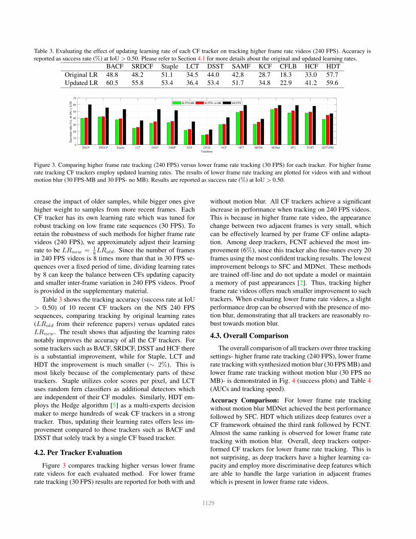
Table 3. Evaluating the effect of updating learning rate of each CF tracker on tracking higher frame rate videos (240 FPS). Accuracy is
reported as success rate (%) at IoU > 0.50. Please refer to Section 4.1 for more details about the original and updated learning rates.
BACF SRDCF Staple LCT DSST SAMF KCF CFLB HCF HDT
Original LR 48.8 48.2 51.1 34.5 44.0 42.8 28.7 18.3 33.0 57.7
Updated LR 60.5 55.8 53.4 36.4 53.4 51.7 34.8 22.9 41.2 59.6
BACF SRDCF Staple LCT DSST SAMF KCF CFLB HCF HDT MEEM MDNet SFC FCNT GOTURN
Trackers
0
10
20
30
40
50
60
70
Success r
ate
(%
), a
t Io
U >
0.5
0
30 FPS-MB 30 FPS- no MB 240 FPS
Figure 3. Comparing higher frame rate tracking (240 FPS) versus lower frame rate tracking (30 FPS) for each tracker. For higher frame
rate tracking CF trackers employ updated learning rates. The results of lower frame rate tracking are plotted for videos with and without
motion blur (30 FPS-MB and 30 FPS- no MB). Results are reported as success rate (%) at IoU > 0.50.
crease the impact of older samples, while bigger ones give
higher weight to samples from more recent frames. Each
CF tracker has its own learning rate which was tuned for
robust tracking on low frame rate sequences (30 FPS). To
retain the robustness of such methods for higher frame rate
videos (240 FPS), we approximately adjust their learning
rate to be LRnew = 1
8LRold. Since the number of frames
in 240 FPS videos is 8 times more than that in 30 FPS se-
quences over a fixed period of time, dividing learning rates
by 8 can keep the balance between CFs updating capacity
and smaller inter-frame variation in 240 FPS videos. Proof
is provided in the supplementary material.
Table 3 shows the tracking accuracy (success rate at IoU
> 0.50) of 10 recent CF trackers on the NfS 240 FPS
sequences, comparing tracking by original learning rates
(LRold from their reference papers) versus updated rates
LRnew. The result shows that adjusting the learning rates
notably improves the accuracy of all the CF trackers. For
some trackers such as BACF, SRDCF, DSST and HCF there
is a substantial improvement, while for Staple, LCT and
HDT the improvement is much smaller (∼ 2%). This is
most likely because of the complementary parts of these
trackers. Staple utilizes color scores per pixel, and LCT
uses random fern classifiers as additional detectors which
are independent of their CF modules. Similarly, HDT em-
ploys the Hedge algorithm [5] as a multi-experts decision
maker to merge hundreds of weak CF trackers in a strong
tracker. Thus, updating their learning rates offers less im-
provement compared to those trackers such as BACF and
DSST that solely track by a single CF based tracker.
4.2. Per Tracker Evaluation
Figure 3 compares tracking higher versus lower frame
rate videos for each evaluated method. For lower frame
rate tracking (30 FPS) results are reported for both with and
without motion blur. All CF trackers achieve a significant
increase in performance when tracking on 240 FPS videos.
This is because in higher frame rate video, the appearance
change between two adjacent frames is very small, which
can be effectively learned by per frame CF online adapta-
tion. Among deep trackers, FCNT achieved the most im-
provement (6%), since this tracker also fine-tunes every 20
frames using the most confident tracking results. The lowest
improvement belongs to SFC and MDNet. These methods
are trained off-line and do not update a model or maintain
a memory of past appearances [2]. Thus, tracking higher
frame rate videos offers much smaller improvement to such
trackers. When evaluating lower frame rate videos, a slight
performance drop can be observed with the presence of mo-
tion blur, demonstrating that all trackers are reasonably ro-
bust towards motion blur.
4.3. Overall Comparison
The overall comparison of all trackers over three tracking
settings- higher frame rate tracking (240 FPS), lower frame
rate tracking with synthesized motion blur (30 FPS MB) and
lower frame rate tracking without motion blur (30 FPS no
MB)- is demonstrated in Fig. 4 (success plots) and Table 4
(AUCs and tracking speed).
Accuracy Comparison: For lower frame rate tracking
without motion blur MDNet achieved the best performance
followed by SFC. HDT which utilizes deep features over a
CF framework obtained the third rank followed by FCNT.
Almost the same ranking is observed for lower frame rate
tracking with motion blur. Overall, deep trackers outper-
formed CF trackers for lower frame rate tracking. This is
not surprising, as deep trackers have a higher learning ca-
pacity and employ more discriminative deep features which
are able to handle the large variation in adjacent frames
which is present in lower frame rate videos.
1129

0 0.1 0.2 0.3 0.4 0.5 0.6 0.7 0.8 0.9 1
Overlap threshold
0
10
20
30
40
50
60
70
80
Success r
ate
(%
)
MDNet [42.9]
HDT [40.3]
SFC [40.1]
FCNT [39.7]
SRDCF [35.1]
BACF [34.1]
GOTURN [33.4]
Staple [33.3]
MEEM [29.7]
HCF [29.5]
SAMF [29.3]
DSST [28.0]
LCT [23.8]
KCF [21.8]
CFLB [14.3]
0 0.1 0.2 0.3 0.4 0.5 0.6 0.7 0.8 0.9 1
Overlap threshold
0
10
20
30
40
50
60
70
80
Success r
ate
(%
)
MDNet [44.4]
SFC [42.3]
HDT [41.4]
FCNT [40.6]
GOTURN [37.8]
SRDCF [35.8]
BACF [35.3]
Staple [34.5]
MEEM [32.9]
SAMF [30.3]
HCF [30.2]
DSST [29.5]
LCT [24.9]
KCF [22.3]
CFLB [14.9]
0 0.1 0.2 0.3 0.4 0.5 0.6 0.7 0.8 0.9 1
Overlap threshold
0
10
20
30
40
50
60
70
80
Success r
ate
(%
)
BACF [49.6]
HDT [47.8]
SFC [47.8]
MDNet [47.3]
SRDCF [47.1]
FCNT [46.9]
Staple [45.3]
DSST [44.8]
SAMF [43.9]
HCF [39.5]
GOTURN [38.6]
MEEM [37.5]
LCT [34.4]
KCF [33.3]
CFLB [19.9]
(a) (b) (c)
Figure 4. Evaluating trackers over three tracking scenarios, (a) lower frame rate tracking with synthesized motion blur, (b) and lower frame
rate tracking without motion blur, and (c) higher frame rate tracking. AUCs are reported in brackets.
Table 4. Comparing trackers on three tracking scenarios including higher frame rate tracking (240 FPS), lower frame rate tracking with
synthesized motion blur (30 FPS MB) and lower frame rate tracking without motion blur (30 FPS no MB). Results are reported as the
AUC of success plots. We also show the speed of each tracker on CPUs and/or GPUs if applicable. The first, second, third, forth and fifth
highest AUCs/speeds are highlighted in color.
BACF SRDCF Staple LCT DSST SAMF KCF CFLB HCF HDT MEEM MDNet SFC FCNT GOTURN
30 FPS- no MB 35.2 35.7 34.5 24.8 29.4 30.3 22.3 14.9 30.2 41.3 32.9 44.4 42.3 40.5 37.7
30 FPS- MB 34.0 35.1 33.2 23.7 28.0 29.2 21.7 14.2 29.5 40.3 29.6 42.9 40.1 39.7 33.4
240 FPS 49.5 47.1 45.3 34.3 44.8 43.9 33.3 19.9 39.5 47.8 37.5 47.3 47.7 46.9 38.6
Speed (CPU) 38.3 3.8 50.8 10.0 12.5 16.6 170.4 85.1 10.8 9.7 11.1 0.7 2.5 3.2 3.9
Speed (GPU) - - - - - - - - - 43.1 - 2.6 48.2 51.8 155.3
Surprisingly, the best accuracy of higher frame rate
tracking achieved by BACF (49.56), which is a CF tracker
with HOG features, followed by HDT (47.80)- a CF tracker
with deep features. SRDCF (47.13), Staple (45.34), DSST
(44.80) and SAMF (43.92) outperformed GOTURN (38.65)
and obtained very competitive accuracy compared to other
deep trackers including SFC (47.78), MDNet (47.34) and
FCNT (46.94). This implies that when higher frame rate
videos are available, the ability of CF trackers to adapt on-
line is of greater benefit than higher learning capacity of
deep trackers. The reasoning for this is intuitive, since
for higher frame rate video there is less appearance change
among consecutive frames, which can be efficiently mod-
eled by updating the tracking model at each frame even us-
ing simple hand-crafted features.
Run-time Comparison: The tracking speed of all evalu-
ated methods in FPS is reported in Table 4. For the sake
of fair comparison, we tested MATLAB implementations
of all methods (including deep trackers) on a 2.7 GHz Intel
Core i7 CPU with 16 GB RAM. We also reported the speed
of deep trackers on nVidia GeForce GTX Titan X GPU to
have a better sense of their run-time when GPUs are avail-
able. On CPUs, all CF trackers achieved much higher speed
compared to all deep trackers, because of their shallow ar-
chitecture and efficient computation in the Fourier domain.
Deep trackers on CPUs performed much slower than CFs,
with the exception of SRDCF (3.8 FPS). On GPU, how-
ever, deep trackers including GOTURN (155.3 FPS), FCNT
(51.8 FPS) and SFC (48.2 FPS) performed much faster than
on CPU. Their performance is comparable with many CF
trackers running on CPU, such as KCF (170.4 FPS), BACF
(38.3 FPS) and Staple (50.8 FPS). For tracking lower frame
rate videos, only BACF, Staple, KCF and CFLB can track at
or above real time on CPUs. GOTURN, FCNT and SFC of-
fer real-time tracking of lower frame rate videos on GPUs.
KCF (170.4 FPS) and GOTURN (155.3 FPS) are the only
trackers which can track higher frame rate videos almost
real time on CPUs and GPUs, respectively.
4.4. Attribute-based Evaluation
The attribute based evaluation of all trackers on three
tracking settings is shown in Fig. 6 (success rate at IoU >
0.50) and Table 5 (relative improvement). Similar to the
previous evaluation, the presence of motion blur slightly
degrades the performance of tracking lower frame rate se-
quences. For lower frame rate tracking, in general, deep
trackers outperformed CF trackers over all nine attributes,
MDNet outperformed SFC and FCNT, and HDT achieved
the superior performance compared to other CF trackers for
all attributes. Compared to lower frame rate tracking, track-
ing higher frame rate videos offers a notable improvement
of all trackers on all attributes except non-rigid deforma-
tion. This demonstrates the sensitivity of both CF based
and deep trackers to non-rigid deformation even when they
track higher frame rate videos. Fig. 6 shows that CF trackers
with hand-crafted features outperformed all deep trackers as
well as HDT for 6 attributes. More particularly, for illumi-
nation variation, occlusion, fast motion, out-of-view, back-
1130

SRDCF (soccer ball)
HDT (pingpong)
MDNet (tiger)
failure case (fish)
Figure 5. Rows(1-3) show tracking result of three trackers includ-
ing a CF tracker with HOG (SRDCF), a CF tracker with deep fea-
tures (HDT) and a deep tracker (MDNets), comparing lower frame
rate (green boxes) versus higher frame rate (red boxes) tracking.
Ground truth is shown by blue boxes. Last row visualizes a failure
case of higher frame rate tracking caused by non-rigid deformation
for BACF, Staple, MDNet and SFC.
ground clutter and low resolution CF trackers with hand-
crafted features (e.g. BACF and SRDCF) achieved superior
performance to all deep trackers and HDT. However, deep
tracker MDNet achieved the highest accuracy for scale vari-
ation (61.0), deformation (59.2) and view change (55.9),
followed by BACF for scale variation (60.1) and HDT for
deformation (57.6) and view change (54.8). The relative im-
provement of tracking higher frame rate versus lower frame
rate videos (with motion blur) is reported in Table 5.
4.5. Discussion and Conclusion
In this paper, we introduce the first higher frame rate ob-
ject tracking dataset and benchmark. We empirically evalu-
ate the performance of the state-of-the-art trackers with re-
spect to two different capture frame rates (30 FPS vs. 240
FPS), and find the surprising result that at higher frame
Table 5. Relative improvement (%) of high frame rate tracking
versus low frame rate tracking for each attribute.
IV SV OCC DEF FM VC OV BC LR
BACF 45.2 31.7 33.1 8.5 39.7 13.4 39.2 25.9 52.7
SRDCF 21.5 15.4 21.9 6.7 31.9 16.4 13.6 32.3 26.1
Staple 41.4 21.4 21.8 7.8 29.7 12.6 25.4 7.1 28.7
LCT 16.1 7.1 18.0 5.4 17.4 8.9 7.8 20.3 26.1
DSST 38.5 30.0 26.4 9.1 35.0 19.0 26.3 25.4 17.7
SAMF 33.8 24.0 26.2 8.7 34.8 13.5 26.0 23.5 15.9
KCF 19.5 10.0 16.6 1.7 21.9 7.8 7.6 15.7 23.7
CFLB 11.1 10.9 10.1 1.0 13.0 2.1 9.1 11.2 14.5
HCF 14.9 9.0 20.2 6.2 19.2 9.4 13.6 20.3 32.0
HDT 22.2 19.5 10.0 5.3 23.6 14.8 25.5 9.4 17.2
MEEM 9.8 7.1 12.8 5.8 16.2 7.1 7.9 9.4 15.3
MDNet 13.1 10.8 8.4 2.7 17.8 13.4 7.2 10.9 6.4
SFC 24.3 19.9 14.8 9.3 23.5 14.7 20.7 13.5 15.0
FCNT 21.8 19.2 12.1 5.9 22.0 15.5 20.5 8.2 13.7
GOTURN 26.1 17.4 8.5 -3.1 20.8 12.2 20.3 12.4 -3.6
rates, simple trackers such as correlation filters trained on
hand-crafted features (e.g. HOG) can achieve very compet-
itive accuracy compared to complex trackers based on deep
architecture. This suggests that computationally tractable
methods such as cheap CF trackers in conjunction with
higher capture frame rate videos can be utilized to effec-
tively perform object tracking on devices with limited pro-
cessing resources such as smart phones, tablets, drones, etc.
As shown in Fig. 7, cheaper trackers on higher frame rate
video (e.g. KCF and Staple) have been demonstrated as
competitive with many deep trackers on lower frame rate
videos (such as HDT and FCNT).
Our results also suggest that traditional evaluation crite-
ria that trades off accuracy versus speed (e.g., Fig.7 in [19])
could possibly paint an incomplete picture. This is because,
up until now, accuracy has been measured without regard to
the frame rate of the video. As we show, this dramatically
underestimates the performance of high-speed algorithms.
In simple terms: the accuracy of a 240 FPS tracker cannot
be truly appreciated until it is run on a 240 FPS video! From
an embedded-vision perspective, we argue that the acquisi-
tion frame rate is a resource that should be explicitly traded
off when designing systems, just as is hardware (GPU vs
CPU). Our new dataset allows for, the first time, exploration
of such novel perspectives. Our dataset fills a need, the need
for speed.
Acknowledgment: This research was supported by the
NSF (CNS-1518865 and IIS-1526033) and the DARPA
(HR001117C0051). Additional support was provided by
the Intel Science and Technology Center for Visual Cloud
Systems, Google, and Autel Robotics. Any opinions, find-
ings, conclusions or recommendations expressed in this
work are those of the authors and do not reflect the view(s)
of their employers or the above-mentioned funding sources.
1131

30 FPS MB 30 FPS- no MB 240 FPS
Background clutter Scale variation Occlusion
0
10
20
30
40
50
60
Success r
ate
(%
), IoU
> 0
.50
BACF
SRDCF
Staple
LCT
DSST
SAMF
KCF
CFLB
HCF
HDT
MEEM
MDNet
SFC
FCNT
GOTU
RN
0
20
40
60
80
Success r
ate
(%
), IoU
> 0
.50
BACF
SRDCF
Staple
LCT
DSST
SAMF
KCF
CFLB
HCF
HDT
MEEM
MDNet
SFC
FCNT
GOTU
RN
0
10
20
30
40
50
60
Success r
ate
(%
), IoU
> 0
.50
BACF
SRDCF
Staple
LCT
DSST
SAMF
KCF
CFLB
HCF
HDT
MEEM
MDNet
SFC
FCNT
GOTU
RN
Illumination variation Fast motion Out-of-view
0
20
40
60
80
Success r
ate
(%
), IoU
> 0
.50
BACF
SRDCF
Staple
LCT
DSST
SAMF
KCF
CFLB
HCF
HDT
MEEM
MDNet
SFC
FCNT
GOTU
RN
0
20
40
60
80
Success r
ate
(%
), IoU
> 0
.50
BACF
SRDCF
Staple
LCT
DSST
SAMF
KCF
CFLB
HCF
HDT
MEEM
MDNet
SFC
FCNT
GOTU
RN
0
20
40
60
80
Success r
ate
(%
), IoU
> 0
.50
BACF
SRDCF
Staple
LCT
DSST
SAMF
KCF
CFLB
HCF
HDT
MEEM
MDNet
SFC
FCNT
GOTU
RN
Deformation Viewpoint change Low resolution
0
20
40
60
80
Success r
ate
(%
), IoU
> 0
.50
BACF
SRDCF
Staple
LCT
DSST
SAMF
KCF
CFLB
HCF
HDT
MEEM
MDNet
SFC
FCNT
GOTU
RN
0
10
20
30
40
50
60
Success r
ate
(%
), IoU
> 0
.50
BACF
SRDCF
Staple
LCT
DSST
SAMF
KCF
CFLB
HCF
HDT
MEEM
MDNet
SFC
FCNT
GOTU
RN
0
20
40
60
80
Success r
ate
(%
), IoU
> 0
.50
BACF
SRDCF
Staple
LCT
DSST
SAMF
KCF
CFLB
HCF
HDT
MEEM
MDNet
SFC
FCNT
GOTU
RN
Figure 6. Attribute based evaluation. Results are reported as success rate (%) at IoU > 0.50.
BACF-LFR tracking-CPU
BACF-HFR tracking-CPU
SRDCF-LFR tracking-CPU
SRDCF-HFR tracking-CPU
Staple-LFR tracking-CPU
Staple-HFR tracking-CPU
SAMF-LFR tracking-CPU
SAMF-HFR tracking-CPU
SAMF-HFR tracking-CPU
KCF-LFR tracking-CPU
KCF-HFR tracking-CPU
HDT-LFR tracking-CPU
HDT-HFR tracking-CPU
HDT-HFR tracking-GPU
HDT-LFR tracking-GPU
MDNet-LFR tracking-CPU
MDNet-HFR tracking-CPU
MDNet-HFR tracking-GPU
MDNet-HFR tracking-CPU
MDNet-HFR tracking-GPU
MDNet-LFR tracking-GPU
SFC-LFR tracking-CPU
SFC-HFR tracking-CPU
SFC-HFR tracking-GPU
SFC-LFR tracking-GPU
FCNT-LFR tracking-CPU
FCNT-HFR tracking-CPU
FCNT-HFR tracking-GPU
FCNT-HFR tracking-CPU
FCNT-HFR tracking-GPU
FCNT-LFR tracking-GPU
Goturn-LFR tracking-CPU
Goturn-HFR tracking-CPU
Goturn-HFR tracking-GPU
Goturn-LFR tracking-GPU
10-3
10-2
10-1
100
101
Real-time performance
20
25
30
35
40
45
50
Su
cce
ss r
ate
(%
)
Figure 7. This plot shows the affect of resource availability (GPUs vs. CPUs) and frame rate of captured videos (lower vs. higher frame
rate) on the top-10 evaluated trackers accuracy and real-time performance. Real-time performance is computed as the ratio of each tracker’s
speed (FPS) to frame rate of the target videos (30 vs. 240 FPS). The vertical line on the plot shows the boundary of being real-time (frame
rate of the target video is the same as the tracker’s speed). Trackers which are plotted at the left side of the line are not able to track
real-time (according to their tracking speed and video frame rate). GPU results are highlighted in yellow.
1132
References
[1] L. Bertinetto, J. Valmadre, S. Golodetz, O. Miksik, and
P. H. S. Torr. Staple: Complementary learners for real-time
tracking. In CVPR, June 2016. 1, 2, 3, 4
[2] L. Bertinetto, J. Valmadre, J. F. Henriques, A. Vedaldi, and
P. H. Torr. Fully-convolutional siamese networks for object
tracking. In ECCV, pages 850–865, 2016. 1, 2, 3, 4, 5
[3] D. S. Bolme, J. R. Beveridge, B. A. Draper, and Y. M. Lui.
Visual object tracking using adaptive correlation filters. In
CVPR, pages 2544–2550. IEEE, 2010. 1, 2, 4
[4] W. Bouachir and G.-A. Bilodeau. Part-based tracking via
salient collaborating features. In WACV, pages 78–85. IEEE,
2015. 3
[5] K. Chaudhuri, Y. Freund, and D. J. Hsu. A parameter-free
hedging algorithm. In NIPS, pages 297–305, 2009. 5
[6] N. Dalal and B. Triggs. Histograms of oriented gradients for
human detection. In CVPR, volume 1, pages 886–893, 2005.
2, 3
[7] M. Danelljan, G. Hager, F. Khan, and M. Felsberg. Accurate
scale estimation for robust visual tracking. In BMVC, 2014.
3, 4
[8] M. Danelljan, G. Hager, F. Shahbaz Khan, and M. Fels-
berg. Convolutional features for correlation filter based vi-
sual tracking. In CVPR Workshop, pages 58–66, 2015. 2,
3
[9] M. Danelljan, G. Hager, F. Shahbaz Khan, and M. Felsberg.
Learning spatially regularized correlation filters for visual
tracking. In ICCV, pages 4310–4318, 2015. 1, 3, 4
[10] M. Danelljan, A. Robinson, F. S. Khan, and M. Felsberg.
Beyond correlation filters: Learning continuous convolution
operators for visual tracking. In ECCV, pages 472–488,
2016. 2, 3
[11] M. Danelljan, F. Shahbaz Khan, M. Felsberg, and J. Van de
Weijer. Adaptive color attributes for real-time visual track-
ing. In CVPR, pages 1090–1097, 2014. 1, 3
[12] A. Handa, R. A. Newcombe, A. Angeli, and A. J. Davison.
Real-time camera tracking: When is high frame-rate best?
In ECCV, pages 222–235, 2012. 2
[13] D. Held, S. Thrun, and S. Savarese. Learning to track at 100
fps with deep regression networks. In ECCV, 2016. 3, 4
[14] J. F. Henriques, R. Caseiro, P. Martins, and J. Batista. High-
speed tracking with kernelized correlation filters. PAMI,
37(3):583–596, 2015. 1, 2, 3, 4
[15] H. Kiani Galoogahi, A. Fagg, and S. Lucey. Learning
background-aware correlation filters for visual tracking. In
ICCV, 2017. 3, 4
[16] H. Kiani Galoogahi, T. Sim, and S. Lucey. Multi-channel
correlation filters. In ICCV, pages 3072–3079, 2013. 1
[17] H. Kiani Galoogahi, T. Sim, and S. Lucey. Correlation filters
with limited boundaries. In CVPR, pages 4630–4638, 2015.
1, 3, 4
[18] M. Kristan, J. Matas, A. Leonardis, and et al. The visual ob-
ject tracking vot2014 challenge results. In ECCV Workshop,
2014. 2, 3
[19] M. Kristan, J. Matas, A. Leonardis, M. et alFelsberg, L. Ce-
hovin, G. Fernandez, T. Vojir, G. Hager, G. Nebehay, and
R. Pflugfelder. The visual object tracking vot2015 challenge
results. In ICCV Workshop, pages 1–23, 2015. 2, 3, 7
[20] A. Krizhevsky, I. Sutskever, and G. E. Hinton. Imagenet
classification with deep convolutional neural networks. In
NIPS, pages 1097–1105, 2012. 3
[21] B. V. Kumar. Correlation pattern recognition. Cambridge
University Press, 2005. 2
[22] Y. Li and J. Zhu. A scale adaptive kernel correlation filter
tracker with feature integration. In ECCV, pages 254–265,
2014. 4
[23] P. Liang, E. Blasch, and H. Ling. Encoding color informa-
tion for visual tracking: algorithms and benchmark. ITIP,
24(12):5630–5644, 2015. 1, 2, 3
[24] C. Ma, J.-B. Huang, X. Yang, and M.-H. Yang. Hierarchical
convolutional features for visual tracking. In CVPR, pages
3074–3082, 2015. 2, 3, 4
[25] C. Ma, X. Yang, C. Zhang, and M.-H. Yang. Long-term
correlation tracking. In CVPR, pages 5388–5396, 2015. 3, 4
[26] M. Mueller, N. Smith, and B. Ghanem. A benchmark and
simulator for uav tracking. In ECCV, pages 445–461, 2016.
2, 3
[27] H. Nam and B. Han. Learning multi-domain convolutional
neural networks for visual tracking. 2016. 2, 3, 4
[28] P. Perez, C. Hue, J. Vermaak, and M. Gangnet. Color-based
probabilistic tracking. Computer visionECCV 2002, pages
661–675, 2002. 3
[29] Y. Qi, S. Zhang, L. Qin, H. Yao, Q. Huang, J. Lim, and M.-H.
Yang. Hedged deep tracking. In CVPR, pages 4303–4311,
2016. 3, 4
[30] K. Simonyan and A. Zisserman. Very deep convolutional
networks for large-scale image recognition. arXiv preprint
1409.1556, 2014. 3
[31] A. W. Smeulders, D. M. Chu, R. Cucchiara, S. Calderara,
A. Dehghan, and M. Shah. Visual tracking: An experimental
survey. TPAMI, 36(7). 2, 3
[32] R. Tao, E. Gavves, and A. W. Smeulders. Siamese instance
search for tracking. arXiv preprint 1605.05863, 2016. 2
[33] C. Vondrick, D. Patterson, and D. Ramanan. Efficiently scal-
ing up crowdsourced video annotation. IJCV, 101(1):184–
204, 2013. 4
[34] L. Wang, W. Ouyang, X. Wang, and H. Lu. Visual tracking
with fully convolutional networks. In ICCV, pages 3119–
3127, 2015. 2, 3, 4
[35] L. Wang, W. Ouyang, X. Wang, and H. Lu. Stct: Sequen-
tially training convolutional networks for visual tracking.
CVPR, 2016. 2
[36] N. Wang and D.-Y. Yeung. Learning a deep compact image
representation for visual tracking. In NIPS, 2013. 3
[37] Y. Wu, J. Lim, and M.-H. Yang. Online object tracking: A
benchmark. In CVPR, pages 2411–2418, 2013. 1, 2, 3, 4
[38] Y. Wu, J. Lim, and M.-H. Yang. Object tracking benchmark.
PAMI, 37(9):1834–1848, 2015. 1, 2, 3
[39] W. Xiang and Y. Zhou. Part-based tracking with appearance
learning and structural constrains. In International Con-
ference on Neural Information Processing, pages 594–601.
Springer, 2014. 3
1133

[40] J. Zhang, S. Ma, and S. Sclaroff. MEEM: robust tracking
via multiple experts using entropy minimization. In ECCV,
pages 188–203, 2014. 4
[41] L. Zhao, X. Li, J. Xiao, F. Wu, and Y. Zhuang. Metric learn-
ing driven multi-task structured output optimization for ro-
bust keypoint tracking. In AAAI, pages 3864–3870, 2015.
3
1134