Embed Size (px)
Citation preview

NEAR EAST UNIVERSITY
Faculty of Engineering
Department of Electrical & Electronic Engineering
Radar In Military Services
Graduation Project EE-400
Student: Anwar Sarsour(981403)
Supervisor: Assoc. Prof. Dr: Sameer lkhdair
t.efkosa - 2001
TABLE OF CONTENST
A.CK.i'IOWLIGMENT
LIST OF ABBREV ATIONS
ABSTRACT
INTRODUCTION
I. BASIC PRINCIPLES
ii
iv
V
1.1 Basic Radar System
1.1.1 Development of Radar
1.1.2 Frequencies and Power Used in Radar 1.2 Radar Performance Factor
1.2.1 Factors ,Influencing Maximum Range 1.2.2 Effect of Noise 1.2.3 Target Properties
2. PULSED SYSTEM 2.1 Basic Pulsed Radar
2.1.1 Receiver Bandwidth Requirements 2.1.2 Factors Governing Pulse Characteristics.
2.2 Antennas and Scanning 2.2.1 Antenna Scanning 2.2 .. 2. Antenna Tracking
2.3 Display Methods 2.4 Pulsed Radar System
2.4.1 Search Radar Systems 2.4.1 Tracking Radar Systems
2.5 Moving Target Indicator (MTI) 2.5.1 Fundamentals of MTI 2.5.2- Other Analog MTI System 2.5.3 Delay Lines 2.5.4 Blind Speeds 2.5.5 Digital MTI
2.6 Radar Beacons 3. OTHER RADAR SYSTEMS
3.1 CW Doppler Radar 3.2 Frequency-Modulated CW Radar 3.3 Phased Array Radars 3.4 Planar Array Radar
4. MILITARY DEFENSE AND ATTACK 4.1 Air Defense
4.1.1 Radar in World War II 4.1.2 Radar during the Cold War
4.2 Radar Systems Classification Methods 4.2.1 World War II Radars
4.2.1.1 AN/TPS-lB, 1 C, 1 D 4.2.1.2 AN/CPS-4 4.2.1.3 AN/CPS-5
2
5
7 8 10 1 l 14 15 15 18 19 21 22 23 26 29 29 30 31 33 36 36 37 38 38 41 41 44 46 50 53 53 55 55 56 56 57 57 57
4.2. l .4 AN/CPS-6. 6A. 68 4.2.1.S AN/TPS-10. 1 OA I AN/FPS-4
-J..2.2 Early Cold War Search Radars 4.2.2. l AN/FPS-3, 3A 4.2.2.2 AN/FPS-5 4.2.2.3 AN/FPS-8 4.2.2.4 AN/FPS-10
4.2.3 SAGE System Compatible Search Radars 4.2.3. l AN/FPS- 7. 7 A. 78. 7CI 70 4.2.3.2 AN/FPS-20,20A, 208 4.2.3.3 AN/FPS-24 4-.2.3.4 AN/IFPS-27.27 A 4.2 .. 3.5 AN/FPS-28 4.2.3.6 AN/FPS-30 4.2.3.7 AN/FPS-31 4.2.3.8 AN/FPS-35 4.2.3.9 AN/FPS-64, 65, 66, 67, 67 A. 72 4.2.3.10 AN/FPS-87 A 4.2.3.11 AN/IFPS-88 4-.2.3 .12 AN/IFPS-91 4.2.3.13 AN/IFPS-93 4-.2.3 .14- AN/IFPS-100 4.2.3 .15 AN/IFPS-100 4.2 .. 3 .16 AN/IFPS-6,6A, 68 4.2.3.17 AN/FPS-26 4.2.3.18 AN/FPS-89 4.2.3.19 AN/FPS-90 4-.2.3 .20 A.N/FPS-116 4.2.3.21 Gap-Filler Radars 4.2.3.22 AN/FPS-14- 4.2.3.23 AN/FPS-18 4.2.3.24 AN/FPS-19
4.2.4 North Warning System Radars 4.2.4.1 AN/FPS-117 4.2.4.2 AN/FPS-124 4.2.4.3 AN/FSS-7 4.2.4.4 AN/FPS-1 7 4.2.4.5 AN/FPS-49, 49A 4.2.4.6 AN!FPS-50 4.2.4. 7 AN/FPS-85 4.2.4.8 ANIFPS-92 4.2.4.9 AN/FPS-108 (Cobra Dane) 4.2.4.10 AN/FPS-115 4.2.4.11 AN/FPS-118 (OTH-B) 4.2.4.12 PARCS
4.3 Missile Detection and Defense 4.4 Ballistic Missile Early Warning System (BMEWS) Radars
4.4.1 AN/FSS- 7 4.4.2AN/FPS-l 7 4.4.3 AN/FPS-49, 49A
58 58 59 59 59 59 59 60 60 60 61 61 61 61 61 62 62 62 62 62 63 63 63 63 63 63 64 64 64 64 64 65 65 65 65 65 66 66 66 67 67 67 67 68 68 68 75 75 75 75

-.-..-t .-'\N/FPS-50 -A.5 .-\N/FPS-85 -.-1.6 AN/FPS-92 -.J.. 7 AN/FPS-108 (Cobra Dane) -.~.8 AN/FPS-1 15 ~.4.9 ANIFPS-118 (OTH-8) .4.10 PARCS
~.5 Federal Aviation Administration (FAA) Radars 4.5 .1 ARSR-1 4.5.2 ARSR-2 -L5.3 ARSR-3, 30 4.5.4 ARSR-4
4.6 Command And Control Systems 4.6.1 Backup Interceptor Control (BUIC) System
CONCLUSION
REFERENCES
76 76 76 77 77 77 77 78 78 78 78 78 79 79 80
82

ACKNOWLEGMENTS
First of all I would like to thank my supervisor Assoc. Prof. Dr. Smeer lkhdair
who has helped me to finish and realize this difficult task, In each discussion, he
explained my questions patiently, and I fell my quick progress from his advises. I asked
him many questions about radar and he always answered my questions quickly and in
detail. To my own Prof Dr. Fakhredden Mamedov who is the Dean of Engineering
Faculty to all his participate. Also thanks to Dr. Kadri, Mr. Ozgur, Mr. Maherdad and all of my other teachers for
their advises. To my friends in N.E.U: Yousif Al-Jazzar, Belal Al-yazji, Moheeb Abu-
Alqumbouz, and special thanks to Taysser Shehada who helped me very much in
completing this project. To my brother and sisters, my sincere thanks are beyond words for their
continuous encouragement. Finally, I am deeply indebted to my parents. Without their endless support and
love for me, I would never achieve my current position. I wish my mother lives happily
always, and my father in the heaven be proud of me.
To all of them, all my love.
1

INTRODUCTION
We had thought to do our work on the radar system, and then we search for the
important part on this subject since the military radar system is one of the most common
and important parts in the communication system.
In 1888 Heinrich Hertz showed that the invisible electromagnetic waves radiated
by suitable electrical circuits travel with the speed of light, and that they are reflected in
a similar way. From time to time in the succeeding decades it was suggested that these
properties might be used to detect obstacles to navigation, but the first successful
experiments that made use of them were in an entirely different context, namely, to
determine the height of the reflecting layers in the upper atmosphere. One of these
experiments, that of Tuve and Breit, made use of short repeated pulses of radiation, and
this technique was employed in most of the developments of radar.
Electromagnetic radiation travels in empty space at a speed of 2.998 x 10⁸ metes
per second, and in air only slightly less rapidly; we can think of its speed as very nearly
300,000 kilometers per second. This speed is denoted by the letter c. Let us suppose that
a very short pulse of radiation is directed towards an object at a distance r, and that a
small fraction of this is reflected back to the starting point, so that it has traversed the
distance 2r. This will take a time t = 2r/c. Ifwe can measure this time we can determine
an unknown distance to the target: r = 1/2ct. For useful terrestrial distances t is very
small; an object 15 km away, for example, will return a signal in one ten-thousandth of
a second.
In practice we need to know more about the target than its distance; we must
also determine its direction. Arranging an antenna system to project a suitable radiation
pattern that can be rotated in azimuth or elevation does this. As may be deduced from
what follows, a very great deal of ingenuity and engineering skill has been devoted to
the design of radar antennas.
The first successful radar installations in Great Britain in the years 1935 to 1939 used
wavelengths in the 6 to 15 m band, and required very large antennas. Other equipment
developed later used wavelengths of 3 m and 1.5 m; and in 1940 the invention of a new
form of generator, the cavity magnetron, at once made it practicable to employ
1

wavelengths of 10 cm and even less. Nearly all the radar development at the National
Research Council in 1942 and later was done at centimeters wavelengths, universally referred to as microwaves.
In chapter one we are going to talk about the basic principles of the radar, the main
components of it, the development. In this chapter we are going to talk also about the
maximum unambiguous range. Frequencies and power used in radar, performance
factor, factors influencing maximum range, effect of noise, and, target properties.
In chapter two present the Basic pulsed radar, receiver bandwidth requirements,
factors governing pulse characteristics, Antennas and scanning, antenna scanning,
Antenna tracking, Display methods, Pulsed radar system, Moving target indicator
(MTI), and, Radar beacons.
Chapter three explains, shows other radar systems like CW Doppler radar,
frequency-modulated CW radar, phased array radars, and, planar-array radar.
Chapter four is a bout the radar in military uses, from 1888 until now how there
use it , how it was developed, and some examples of it.

CHAPTER ONE
BASIC PRINCIPLES
A typical radar system consists of the following components:
• A pulse generator that discharges timed pulses of UHF microwave/radio energy
• A transmitter
• A duplexer
• A directional antenna that shapes and focuses each pulse into a stream
Returned pulses that the receive antenna picks up and sends to a receiver that
converts (and amplifies) them into video signals
• A recording device which stores them digitally for later processing and/or
produces a real time analog display on a cathode ray tube (CRT) or drives a
moving light spot to record on film.
Each pulse lasts only microseconds (typically there are about 1,500 pulses per
second). Pulse length-an important factor along with bandwidth in setting the system
resolution-is the distance traveled during the pulse generation. The duplexer separates
the outgoing and returned pulses (i.e., eliminates their mutual interferences) by blocking
reception during transmission and vice versa. The antenna on a ground system is
generally a parabolic dish.
Radar antennas on aircraft are usually mounted on the underside of the platform so
as to direct their beam to the side of the airplane in a direction normal to the flight path.
For aircraft, this mode of operation is implied in the acronym SLAR, for Side Looking
Airborne Radar. A real aperture SLAR system operates with a long (about 5.6 m)
antenna, usually shaped as a section of a cylinder wall. This type produces a beam ofno
coherent pulses and uses its length to obtain the desired resolution (related to angular
beam width) in the azimuthally (flight line) direction. At any instant the transmitted
beam propagates outward within a fan-shaped plane, perpendicular to the flight line. A
second type of system, Synthetic Aperture Radar (SAR), is exclusive to moving
1

platforms. It uses an antenna of much smaller physical dimensions, which sends its
pulses from different positions as the platform advances, simulating a real aperture by
integrating the pulse echoes into a composite signal. It is possible through appropriate
processing to simulate effective antenna lengths up to 100 m or more. This system
depends on the Doppler effect ( apparent frequency shift due to the target's or the radar
vehicle's velocity) to determine azimuthally resolution. As coherent pulses transmitted
from the radar source reflect from the ground to the advancing platform (aircraft or
spacecraft), the target acts as if it were in apparent (relative) motion. This motion results
in changing frequencies, which give rise to variations in phase and amplitude in the
returned pulses. The radar records these data for later processing by optical ( using
coherent laser light) or digital correlation methods. The system analyzes the moderated
pulses and recombines them to synthesize signals equivalent to those from a narrow
beam, real-aperture system.
1.1 Basic Radar System The operation of a radar system can be quite complex, but the basic principles are
somewhat easy for the reader to comprehend. Covered here are some fundamentals,
which will make the follow up material easier to digest. In figure (1.1) and timing
diagram (figurel.2). A master timer controls the pulse repetition frequency (PRF).
Theses pulses are transmitted by a highly directional parabolic antenna at the target,
which can reflect (echo) some of the energy back to the same antenna. This antenna has
been switched from a transmit mode to a receiver by a duplexer. The reflected energy is
received, and time measurements are made, to determine the distance to the target. The
pulse energy travels at 186,000 statute miles per second (162,000 nautical miles per
second). For convenience, a radar mile (2000 yd or 6000 ft) is often used, with a little as
1 percent error being introduced by this measurement. The transmitted signal takes 6.16
µs to travel 1 radar mile; therefore the round trip for 1 mile is equal to 12.36 µs. With
this information, the range can be calculated by applying equation (1.1).
L1t Range=-- (1.1) 12.36
t = time from transmitter to receiver in microsecond.
For higher accuracy and shorter range, equation (1.2) can be utilized.
2

328Jt Range (yard)= = l64L'lt
2 (1.2)
Transmitter
Duplexer Antenna
Receiver
Figure 1.1 block diagram of elementary pulsed radar
Pulse repetition time (PRT)
(a)
pulse2
Target 1
370µs
PRR
OrPRF
(b)
Figure 1.2 timing diagram
3

After the radar pulse has been transmitted, a sufficient rest time (figure 1.2a)
(receiver time) must be allowed for the echo to return so as not to interfere the next
transmit pulse. This PRT, or pulse repetition time, determines the maximum distance to
the target to be measured. Any signal arriving after the transmission of the second pulse
is called second return echo and would give ambiguous indications. The range beyond
which objects appear as second return echo is called the maximum unambiguous range
(MUR) and can be calculated as shown in equation (1.3).
PRT mur=-- 12.2
(1.3)
Range in miles; PRT in µs Refer to the timing diagram (figure 1.2a) by calculation, maximum unambiguous
distance between transmit pulse 1 and transmit pulse 2 is 50 mi. Any return pulse
related to transmit 1 outside this framework will appear as weak close-range pulse
related to transmit pulse 2. This distance between pulse 1 and pulse 2 is called the
maximum range.
~ .••.. ~~., .,,.,,. .,.,,. , ,, .... ' .,. .. ~.,,
.,.~~- .. ,. ,,, 1_-; ~ ,. ... ,. ..• ,. ... ~,.
Radar 2
~ False echo
Radar 1 _f\__J\_
True echo
Figure 1.3 Double-range echoes

If a large reflected object is very close, the echo may return before the complete
pulse can be transmitted. To eliminate ambiguity, the receiver is blocked, or returned
off. Blocking of the receiver during the transmit cycle is common in must radar systems.
A second problem arises with large objects at close range. The transmitted pulse may be
reflected by the target for one complete round trip, figure (1.3). It may then, because of
it's high energy level, be reflected by the transmitter antenna and bounced back to the
target for a second round trip. This condition is called double range echoes. To
overcome this form of ambiguity, Equation (1.4) is used to determine the minimum
effective range.
Minimum range = 164 PW
Range = yards
PW=µs
Other terms sometimes discussed in conjunction with the radar transmitter are duty
cycle, peak power, and average power, to calculate the duty cycle the Equation (1.5) can
be used.
PW Duty cycle= PRT (1.5)
We can conclude that in order to produce a strong echo over a maximum range, high
peak power is required. In some situations, size and heat are important factors (in radar
in aircrafts) and low average power is requirement. We can see how low duty cycle is an
important consideration. Commenting briefly on the other aspect of the radar set we find
that the pulse-modulated magnetron, klystrons TWTs or CFAs are normally used as
transmitter output tube, and the first stage of the receiver is often a diode mixer. The
antenna generally uses a parabolic reflector of some form as will be mentioned in
section (2.2).
1.1.1 Development of radar From its inception, radar has used a system of sending powerful pulses of radio
energy and then analyzing the returned echoes to determine the position, distance and
possibly velocity of the target. However, the methods of doing so have evolved and
become far more refined and sophisticated as time has by. The primary incentive was
5

the imminence of war. Radar was made possible technology, which, at the time war
broke out, was just beginning to show promise. This technology itself took great strides
forward to meet the new challenges imposed by war. The first radars worked at much lower frequencies than present systems as 60
MHz for the original British coastal air-warning radar because of sufficiently powerful
transmitting tubes at higher frequencies. This was changed in 1940 with the appearance
of the cavity magnetron, and the stage was then set for the development of modern
radar. One of the prime requirements of a system is that it should have a fair degree of
accuracy in its indication of target direction. This is possible only if the antennas used C'
are narrow-beam ones, i.e., have dimensions of several wavelengths. That requirement
cannot be fulfilled satisfactorily unless the wavelengths themselves are fairly short,
corresponding to the upper UHF or microwave frequencies. The advent of the magnetron also made possible the next steps in the evolution of
radar, namely, airborne radar for the detection of surface vessels and then aircraft
interception radar. In each of these, tight beams are necessary to prevent the receiver
from being swamped by ground reflections, which would happen if insufficient
discrimination between adjacent targets existed. Microwave radar for anti fire control
was quickly developed, of which the most successful ground-based was the U.S.
Army's SCR-584. It was capable of measuring the position of aircraft to within 0.10.
And the distance, or range, to within 25 m. Such radars were eventually capable of
tracking targets by locking onto them, with the aid of servomechanisms controlling the
orientation of the antennas. Anti-surface vessel (ASV) radars became very common and
quite accurate toward the end of the war. So did airborne radar for navigation, bombing
or bomber protection; electronic navigation systems were also developed. Radar
countermeasures were instituted, consisting mainly of jamming (transmission of
confusing signals at enemy radar) or the somewhat more effective dropping of
aluminum foil, in strips of about a half-wavelength, to cover approaching aircraft by
producing false echoes. This "chaff" (American) or ''window" (British) proved very
effective, but its use in the war was considerably delayed. Each side thought that the
other did not know about it and so it was kept secret; however, it eventually came to be
used on a very large scale. One of the indications of the enormous growth in the
6

importance of radar in World War II is the increase in the staff of the U.S. Army's
Radiation Laboratory. It started with about 40 people in 1941, and numbers multiplied
tenfold by 1945. The subsequent developments of radar have also been numerous. They have
included the use of wavelengths well into the millimeter range, at which atmospheric
interference becomes noticeable, but for the presence of radar ''windows." We have
witnessed the use of greater powers at all wavelengths and the use of computers for a
number of applications ( especially fire control) to improve accuracy and reduce the time
lag of manual operation. Long-range, fixed early-warning radars have been built,
including the MEWS and BMEWS systems. These radars use huge antennas and
enormous transmitting powers and are supplemented by radar-carrying high-flying
aircraft, which have an extended radar horizon because of their height. Satellites
carrying radar have been employed for military purposes, such as early detection of
ballistic missiles, and civilian uses, notably in meteorology and mapping. Other
important civilian uses of radar have included coastal navigation for shipping, position
finding for shipping and aircraft, and air-traffic control at airports. This has extended the
use of the landing facilities to weather conditions, which would have made them
unusable without radar and its allied systems. Also, the use of radar by various police
forces, for the control of traffic speed and the prosecution of offenders, is becoming
commonplace. Numerous scientific advances have been made with the aid of radar; for instance,
as early as in 1945 an error of 900 m was found (by accident) in the map position of the
island of Corsica. More recent scientific uses of radar on an interplanetary scale have
yielded much useful information about the sun and the rest of the solar system, and
especially about the distances and rotations of the various planetary bodies. For
example, it is now known that the planet Mercury rotates with a speed not equal to its
angular orbital velocity, so that it does not always present the same face to the sun.
1.1.2 Frequencies and powers used in radar The frequencies employed by radar lie in the upper UHF and microwave ranges. As a
result of wartime security, names grew up for the various frequency ranges, or bands,
7

these are still being used. One such term (the X hand), and the others will now be
identified. Since there is not a worldwide agreement on radar band nomenclature, the
~ used in Table 1-1 are the common American designations.
BAND FREQUENCY RANGE MAXIMUM AVAILABLE
NAME GHz PEAK POWERMW
UHF 0.3- 1.0 5.0
L 1.0-1.5 30.0
s 1.5-3.9 25.0
C 3.9-8.0 15.0
X 8.0-12.5 10.0
KU 12.5-18.0 2.0
K 18.0-26.5 0.6
Ka 26.5-40.0 0.25
V 40.0-80.0 0.12
N 80.0-170.0 0.01
A Above 170 -
Table 1.1 radar bands
1.2 Radar Performance Factor Quite apart from being limited by the curvature of the earth, the maximum
range of radar set depends on a number of other factors. These can now be discussed,
beginning with the classical radar range equation.
To determine the maximum range of radar set, it is necessary to determine
the power of the received echoes, and to compare it with the minimum power that the
receiver can handle and display satisfactorily. If the transmitted pulsed power is f (peak value) and the antenna is isotropic, then the power density at a distance r from the
antenna will he as given by Equation (1.6), namely,
(1.6)
8

However, antennas used in radar are directional, rather than isotropic. If Ap the
maximum power gain of the antenna used for transmission, so the power density at the
target will be
APPt p=-- 4ir r2
(1.7)
The power intercepted by the target depends on its radar cross-section, or effective area,
will be discussed later on. If this area is S. the power impinging on the target will be
A pS p=pS= P 1 (1.8)
4ir r2 the target is not an antenna. It is radiation may be thought of as being omni directional.
The power density of its radiation at the receiving antenna will be
, p App,S p =--2 = 2
4ir r ( 4ir r2) (1.9)
Like the target, the receiving antenna intercepts a portion of the reradiated power,
which is proportional to the cross-sectional area of the receiving antenna. However, it is
the Capture area of the receiving antenna that is used here. Equation (1.10). The
received power is
A rs» P' = P'Ao = P 1 ""()
(4JZT2)2
Where Ao =capture area of the receiving antenna. If (as it is usual the case) the same antenna is used for both reception and transmission,
(1.10)
we have equation ( 1.11) is for the maximum power gain,
A = 47!Ao p A,2
(1.11)
Substituting equation ( 1.11) into ( 1.10) gives
P' = 47rAo P,SAo = P,A0 2 S
1t2 16ir2r4 4nr41t2 the maximum range rmax will be obtained when the received power is equal to the
(1.12)
minimum receivable power of the receiver Pmin. Substituting this into equation (1.12),
and making r subject of the equation, we have
9

rmax =( PrA;S )~ 41rl2 P: mm
(1.13)
Alternatively, if Equation (1.11) is turned around so that Ao =Ai)}/41t is
substituted into Equation (1.13), we have
r =( PrA;i2s J~ max ( 41r/ p min
(1.13a)
Equations (1.13) and (1.13a) represent two convenient forms of the radar range
equation., simplified to the extent that the minimum receivable power Pmin has not yet
been defined. It should also be pointed out that idealized conditions have been
employed. Since neither the effects of the g~ound nor other absorption and interference
have been taken into account, the maximum range in practice is often less than that
indicated by the radar range equation.
1.2.1 Factors influencing maximum range A number of very significant and interesting conclusions may be made if the radar
range equation examined carefully. The first and most obvious is that the maximum
range is proportional to the fourth root of the wok transmitted pulse power. The peak
power must he increased sixteen fold, all else being constant; if a given maximum range
is to he doubled. Eventually, such a power increase obviously becomes uneconomical in
any particular radar system. Equally obviously, a decrease in the minimum receivable power will have the
same effect as raising the transmitting power and is thus a very attractive alternative to
it. However, a number of other factors are involved here. Since Pmin is governed by the
sensitivity of the receiver (which in turn depends on the noise figure), the minimum
receivable power may be reduced by a gain increase of the receiver, accompanied by a
reduction in the noise at its input. Unfortunately, this may make the receiver more
susceptible to jamming and interference, because it now relies more on its ability to
amplify weak signals (which could include the interference), and less on the sheer
power of the transmitted and received pulses. In practice, some optimum between
transmitted power and minimum received power must always be reached.

The reason that the range is inversely proportional to the fourth power of the
transmitted peak power is simply that the signals are subjected twice to the operation of
the inverse square law, once on the outward journey and once on the return trip. By the
same token, any property of the radar system that is used twice, i.e., for both reception
and transmission, will show a double benefit if it is improved. Equation (1.13) shows
that the maximum range is proportional to the square root of the capture area of the
antenna, and is therefore directly proportional to its diameter if the wavelength remains
constant. It is thus apparent that possibly the most effective means of doubling a given
maximum radar system range is to double the effective diameter of the antenna. This is
equivalent to doubling its real diameter if a parabolic reflector is used. Alternatively, a
reduction in the wavelength used, i.e., an increase in the frequency, is almost as
effective. There is" a limit here also. The beam width of an antenna is proportional to the
ratio of the wavelength to the diameter of the antenna. Consequently, any increase in the
diameter-to-wavelength ratio will reduce the beam width. This is very useful in some
radar applications, in which good discrimination between adjoining targets is required,
hut it is a disadvantage in some search radars. It is their function to sweep a certain
portion of the sky, which will naturally take longer as the beam width of the antenna is
reduced. Finally, Equation (1.13) shows that the maximum radar range depends on the
target area, as might be expected. Also, ground interference will limit this range. The
presence of a conducting ground, it will be recalled, has the effect of creating an
interference pattern such that the lowest lobe of the antenna is some degrees above the
horizontal. A distant target may thus be situated in one of the interference zones, and
will therefore not be sighted until it is quite close to the radar set. This explains the
development and emphasis of "ground-hopping" military aircraft, which are able to fly
fast and close to the ground and thus remain undetectable for most of their journey.
1.2.2 Effect of noise The previous section showed that noise affects the maximum radar range insofar
as it determines the minimum power that the receiver can handle. The extent of this can
now be calculated exactly. It is possible to calculate the equivalent noise power
11

generated at the input of the receiver. N; This is the power required at the input of an
ideal receiver having the same noise figure as the practical receiver. We then have
(S/N ); F= (S/NJo
S.N0 S.G(N.+N) N -'-= z .z r =I+_L S0N. GS.N. N.
l l 1 l
(1.14)
Where Si = input signal power
Ni= input noise power
So = output signal power
No= output noise power
G = power gain of the receiver
We have
N _L=F-I N.
l
N = (F-l)N. = kT0<5f(F-1) r z (1.15)
N1 Nr(F- ON1klo8f(F-I)(16-15)
Where kT o&f = noise input power of receiver
k = Bolt Mann's constant 1.38 * 10·23 J/K To = standard ambient temperature I 7°C = 290 K
Sf = bandwidth ofreceiver
It has been assumed that the antenna temperature is equal to the standard ambient
temperature, which may or may not be true; but the actual antenna temperature is of
importance only if a very low-noise amplifier is used. Reference may be made for the
reasoning behind the substitution for Ni.
The minimum receivable signal for the receiver, under so-called threshold de
tection conditions, is equal to the equivalent noise power at the input of the receiver, as
just obtained in Equation ( 1.15), This may seem a little harsh, especially since much
12

higher ratios of signal to noise are used in continuous modulation systems. However, it
must be realized that the echoes from the target are repetitive, whereas noise impulses
are random. An integrating procedure thus takes place in the receiver, and meaningful
echo pulses may be obtained although their amplitude is no greater than that of the noise
impulses. This may be understood by considering briefly the display of the received
pulses on the cathode-ray tube screen. The signal pulses will keep recurring at the same
spot if the target is stationary, so that the brightness at this point of the screen is
maintained (whereas the impulses due to noise are quite random and therefore not
additive). If the target itself is in rapid motion, i.e., moves significantly between
successive scans, a system of moving-target indication ( coming in chapter three) may be
used. Substituting these findings into Equation (1.13), we have
[
2 ]l/4 ~~s r max = 47rA 2 kT0~f (F -1)
(1.16)
Equation (1-16) is reasonably accurate in predicting maximum range, provided that a
number of factors are taken into account when it is used. Among these are system
losses, antenna imperfection, receiver nonlinearties, anomalous propagation, proximity
of other noise sources (including deliberate jamming) and operator errors, and/or fatigue
(if there is an operator). It would be safe to call the result obtained with the aid of this
equation the maximum theoretical range, and to realize that the maximum practical
range varies between 10 and 100 percent of this value. However, range is sometimes
capable of exceeding the theoretical maximum under unusual propagating conditions,
such as super refraction. It is possible to simplify Equation ( 1.16), which is rather cumbersome as it stands.
Substituting for the capture area in terms of the antenna diameter (Ao= 0.651tD2/4) and
for the various constants, and expressing the maximum range in kilometers, allows
simplification to
]
l/4 PD2S
'= =4t,~1(F-I) (1.17)
Where rmax = maximum radar range, Km
13

Pt= peak pulse power, W
D = antenna diameter, m
S = effective cross-sectional area of target, m
of= receiver bandwidth, Hz
"A, = wavelength. M.
F = noise figure ( expressed as ratio).
1.2.3 target properties In connection with the derivation of the radar range equation, a quantity was used hut
not defined. This was the radar cross-section, or effective area, the target. For targets
whose dimensions are large compared to the wavelength, as aircraft microwave radar is
used, the radar cross section may be defined as the objected area of a perfectly
conducting sphere which would reflect the same power as e actual target reflects, if it
were located at the same spot as the target. The practical nation is far from simple.
First of all, the radar cross section depends on the frequency used. If this is such at
the target is small compared to a wavelength. Its cross-sectional area for radar appears
much smaller than its real cross section. Such a situation is referred to as the Raleigh
region. When the circumference of a spherical target is between 1 and 10 wavelengths,
the radar cross section oscillates about the real one. This is the so-called resonance
region. Finally. Fey shorter wavelengths (in the optical region) the radar and e cross
sections are equal. Quite apart from variations with frequency, the radar cross section of a target will
depend on the polarization of the incident wave, the degree of surface roughness (If it is
severe), the use of special coatings on the target and, most importantly of all. The aspect
of the target. For instance, a large jet aircraft, measured at 425 MHz, has found to have a
radar cross section varying between 0.2 and 300 m2 for the fuselage, depending on the
angle at which the radar pulses arrived on it. The situation is seen to be complex
because of the large number of factors involved, so that a lot of work is empirical.
14

CHPTER TWO
PULSED SYSTEMS
Pulse. systems can be descried in some details, starting with the block diagram of a
typical pulse. radar set and its description., followed. by discussion of scanning and
display method. Pulse radar can be divided broadly into search radars and tracking
Trigger Source arite-rma
Out put tube ATR switch TR switch
Modulator
Video amplifier Indicator
Ano le data from antenna
Detector If amplifier Mixer
Local Oscillator
Figure 2.1 pulse radar block diagrams. and some mention can be made of auxiliary systems such as beacon and transponders.
2.1 Basic Pulse Radar System A very elementary block diagram of pulsed radar set was shown in figure ( 1.1) more
detailed block diagram is given and it will be possible to talk a bout the pulsed system
and the circuits used with those. The block diagram of figure (2..1) shows the arrangement of atypical high-pulsed radar
15

set. The trigger source provides pulses for the modulator. The modulator provides
rectangular voltage pulses used as the supply voltage for the output tube, switching it on
and off as required, This tube may be magnetron oscillator or an amplifier such as the
Klystron, traveling wave tube or a crossed field amplifier, depending on specific.
requirements. If an amplifier is used, a source of microwave is required. While an
amplifier may be modulated at a special grid, the magnetron cannot. If the radar is small
powered one, it may use IMP A TT or gun oscillator, or TRAP A TT amplifiers. Bellow c
band. power transistor amplifier or oscillator may also be. used. The transmitter portion
of the radar is terminated with the duplexer, which passes the output. pulse to the
antenna for transmission.
The receiver is connected to the antenna at suitable times (i.e .. when no transmission is
instantaneously taking place). As previously explained, the duplexer also does this. As
shown here, a ( semiconductor diode) mixer is the. most likely first stage in the receiver,
since- it has a fairly low noise figure, but of course it shows a conversion loss. An RF
amplifier can also be used, and this would most likely be a transistoror IC, or perhaps a
tunnel diode or par amp. A better noise figure is thus obtained, and the RF amplifier
may have. the further advantage. of saturating for large signals, thus acting as a limiter
that prevents mixer diode burnout from strong echoes produced by nearby targets. The
main receiver gain is provided. at an. intermediate frequency - that is typically 30 or 60
Ml-lz, However, it may take two or more- down conversions to reach that IF from the
initial microwave. RF, to ensure adequate image frequency suppression.
If diode. mixer is the first stage, the (first) IF amplifier must be designed as a. low
noise stage to ensure-that the overall noise figure of the receiver does not deteriorate. A
noisy IF amplifier would play havoc with the overall receiver performance, especially
when it is noted that the "gain" of a diode mixer is in fact a.conversion loss typically 4.
to 7 dB. A cascade connection is quite common for the transistor amplifiers used in the
IF stage, because it removes the need for neutralization to avoid the Miller effect.
Another source of noise. in the receiver of Figure (1.4) may be the local oscillator,
especially for microwave radar receivers. One of the methods of reducing such noise is
to use a vector or step-recovery diode multiplier. Another method involves the
connection of a narrowband filter between the local oscillator and the mixer to reduce
16

the noise bandwidth of the mixer. However, in receivers employing automatic frequency
correction this may be unsatisfactory. The solution of the oscillator noise problem may
then lie in using a balanced mixer and/or a cavity-stabilized oscillator. If used, AFC
may simply consist of a phase discriminator which takes part of the output from the IF
amplifier and produces a de correcting voltage if the intermediate frequency drifts. The
voltage may then be applied directly to a vector in a diode oscillator cavity.
The IF amplifier is broadband, to permit the use of fairly narrow pulses. This means
that cascaded rather than single-stage amplifiers are used. These can be synchronous
that is. All tuned to the same frequency and having identical band pass characteristics. If
a really large. bandwidth is needed, the individual IF amplifiers may be stagger-tuned
the overall response is achieved by overlapping the, responses of the individual
amplifiers, which are tuned to nearby frequencies on either side of the center frequency.
The- detector is often a Schottky-barrier diode, whose, output is amplified by a video
amplifier having the same bandwidth as the IF amplifier. Its output is then fed to a
display unit, directly or via.computerprocessing and enhancing.
Modulators In a.radar transmirter, the modulator is a circuit or group of circuits whose
function it is to switch the output tube ON and OFF as required. There are two main
types in common use: lint -pulsing modulators and active-switch modulators. The latter
are also known as driver-power-amplifier modulators and. were called hard-tube
modulators until the advent of semiconductor devices capable of handling some modu
lator duties. Here the anode of the output tube (or its collector; depending on the tube used) is
modulated directly by a system that generates and provides large pulses of supply
voltage. Slowly charging and then rapidly discharging a transmission line achieve this
The charging is made slow to reduce the current requirements and is generally done
through an inductance. The transmission line is able to store energy in its distributed
inductance· and capacitance. If the line is charged to a voltage V from a high-impedance
source, this voltage will drop to 1/2V when a load is connected (the output tube) whose
impedance is equal to the characteristic impedance of the line. However, at the instant
of load connection the voltage across the line is 112V only at the input; it is still V
everywhere else. The voltage drop now propagates along the line to the far end, from
17

which it is reflected to the input terminals. It is thus seen that a voltage V will be
maintained across the load for· a time 2t, where t is the time taken by an electromagnetic
wave to travel from one end of the line to the other.
If the pulse duration (2t) is to be 1 µs, the line length must be 150 m. This is far
too long for convenience, and consequently a pulse-farming network (PFN) is almost
always substituted for the transmission line. As shown in Figure (2.2), which illustrates
a very basic modulator, the PFN looks just like the equivalent circuit of a transmission j
line. It also behaves identically to the transmission line for frequencies below f = lhc square root of LC, where Land Care the inductance and capacitance, respectively, per
section. In high-power radars, the device most likely for use as a switch is a hydrogen
thyratron, because it is capable of switching very high powers and of rapid deionization ..
Silicon-controlled rectifiers (SCRs) may also be used to good advantage.
The advantages of the line modulator are that it is simple, compact, reliable and
efficient. However, it has the disadvantage that the PEN must be changed if a different
pulse length is required. Consequently, line modulators are not used at all in radars from
which variable pulse. widths are required, but they are often used. otherwise. The pulses
that are produced have adequately steep sides and. flat tops.
The:active-switch modulator is one that can also provide high-level modulation of the
output tube, but this time: the pulses are generated at a low power level and then
amplified. The driver is often a blocking oscillator; triggered ·by a timing source and
driving an amplifier. Depending on the power level, this may be a transistor amplifier or
a powerful tube such as a shielded-grid triode. The amplifier then controls the De power
supply for the output RF tube. This type of modulator is less efficient, more complex.
and bulkier than the line modulator, but it does have the advantage of easily variable
pulse length, repetition rate or even shape. It is often used in practice.
Finally, low-level modulation is also sometimes possible. This may be done in
UHF radar, which uses orthodox vacuum tubes, or at higher frequencies if a velocity-
modulated amplifier is used. Also, in some low-power radars, it becomes possible to
apply the output of the blocking oscillator directly to the output tube, simplifying the
modulator circuitry. Receiver bandwidth requirements Based on what we learned in Chapter 1. the
18

bandwidth of the receiver correspond to the bandwidth of the transmitter and its pulse
width. The narrower the pulses, the greater is the IF (and video) bandwidth required,
whereas the RF bandwidth is normally greater than these, as in other receivers. With a
given pulse duration T, the receiver bandwidth may still vary, depending on how many
harmonics of the pulse repetition frequency are needed to provide a received pulse
having a suitable shape. If vertical sides are required for the pulses in order to give a
good resolution (as will he seen), a large bandwidth is required. It is seen that the
bandwidth must be increased if more information about the target is required, but too
large a bandwidth will reduce the maximum range by admitting more noise, as shown
by Equation ( 1.16). The IF bandwidth of a radar receiver is made n/T, where· T is the. pulse duration
and n is a number whose value ranges from under 1 to over 10, depending on the
circumstances. Values of n :from I to about 1.4 are the most common. Because pulse
widths normally range from 0.1 to 10 µs, it is seen that the radar receiver bandwidth
may lie in the range from about 200 kHz to over 10 MHz. Bandwidths :from I to 2 MHz
are the most common,
2.1.2 Factors governing pulse characteristics
We. may now consider why flat-Lopped rectangular pulses are preferred in radar and
what it is that governs their amplitude, duration and repetition rate. These factors are of
the greatest importance in specifying and determining the performance of a. radar
system. There are several reasons why radar pulses ideally should have vertical sides and flat
tops. The leading edge of the transmitted pulse must. be vertical to ensure that the
leading edge of the received pulse is also close to vertical. Otherwise, ambiguity will
exist as to the precise instant at which the pulse has been returned, and therefore
inaccuracies will creep into the exact measurement of the target range .. This requirement
is of special importance in fire-control radars. A flat top is required for the voltage pulse
applied to the magnetron anode; otherwise its :frequency will be altered .It also is needed
because the efficiency of the magnetron, multicavity klystron or other amplifier drops
significantly if the supply voltage is reduced. Finally, a steep trailing edge is needed for
19

the transmitted pulse, so that the duplexer can switch the receiver over to the antenna as
soon as the body of the pulse has passed. is will not happen if the pulse decays slowly,
since there w1ll be sufficient pulse power present to keep the TR switch ionized. We see
that a pulse trailing edge, which is not steep, has the effect of lengthening the period of
time, which the receiver is disconnected from the antenna.. Therefore it limits the
minimum range of the radar. This will be discussed in connection with pulse width.
The pulse repetition frequency, or PRF. is governed mainly by two conflicting factors.
The first is the maximum range required, since it is necessary not only to be able to
detect pulses returning from distant targets but also to allow them time to return before
the next pulse. is transmitted .. If given radar is to have a range of 50 nmi (92.6 kin), at
least 620 µs must be allowed. between successive pulses; this period is called the. pulse
interval. Ambiguities will result if this is not done. If only 500 µs is used as the pulse
interval, an echo received 120 µs after the transmission of a pulse could mean either that
the target is 120/12.4 = 9.7 nmi (18 km) away or else that the pulse received is a
reflection of the previously sent pulse, so that the target is (120 + 500)/12.4 = 50 nmi
away. From this point. of view, it is seen that the pulse interval should be as large as
possible. The greater the- number of pulses reflected from a target, the greater the
probability of distinguishing this target from noise. An integrating effect takes place if
echoes repeatedly come from the same target, whereas noise is random .. Since the
antenna moves at a significant speed in many types of radar, and yet it is necessary to
receive several pulses from a given target, a lower limit on the pulse repetition fre
quency clearly exists. Values of PRF from 200 to l 0,000/s are commonly used in
practice, corresponding to pulse intervals of 5000 to 100 µs and therefore to maximum
ranges from 400 to 8 nmi (740 to 15 km). When the targets are very distant (satellites
and. space probes, for example), lower PRFs may have to be used (as low as 30 pps).
If a short minimum range is required, then short pulses must be transmitted. This rs
really a continuation of the argument in favor of a vertical trailing edge for the
transmitted pulse. Since the receiver is disconnected from the antenna for the duration
of the pulse being transmitted (in all radars using duplexers), it follows that echoes
returned during this period cannot be received. If the total pulse duration is 2 µs, then no
pulses can be received during this period. No echoes can be received from targets closer

than 300 m away, and this is the minimum range of the radar. Another argument in
favor of short pulses is that they improve the range resolution, which is the ability to
separate targets whose distance from the transmitter differs only slightly. Angular·
resolution, as the name implies, is dictated by the beam width of the antenna. If the
beam width is 2°, then two separate targets that are less than 2° apart will appear as one
target and will therefore not be resolved. If a pulse duration of 1 µs is used, this means
that echoes returning from separate targets that are 1 µs apart in time, (i.e., about 300 m
in distance) will merge into one returned pulse and will not be separated. It is seen that
the range resolution in this case is no better than 300 m..
It is now necessary to consider some arguments in favor of long pulse durations.
The main one is simply that the receiver bandwidths must be increased as pulses are
made narrower; and Equation (1.16) shows that this tends to reduce the maximum range
by admitting more noise into the system. Increasing the peak pulse power, but only at
the expense of cost, size and power consumption may of course, counteract this. A
careful look at the situation reveals that the maximum range depends on the pulse
energy rather than on its peak power. Since one. of the terms of Equation (L16) is P/8 J and the bandwidth 8 f is Inversely proportional to the pulse duration, we are entitled to say that range depends on the product of PT, and. T, and this product is equal to the
pulse energy. We must keep in mind that increasing the pulse width while keeping a
constant PRF has the effect of increasing the duty cycle of the output tube, and therefore
its average power. As the. name implies, the duty cycle is the fraction of time during
which the output tube. is ON If PRF is 1200 and the pulse width is 1.5 µs, the period of
time actually occupied.by the transmission of pulses is 1200 x 1.5 =1800 µs/s. or 0.0018
(0.18 percent increasing the duty cycle thus increases the dissipation of the output tube.
It may also have the effect of forcing a reduction. in the peak power, because the peak
and average powers are closely related for any type of tube. If large duty cycles are
required, it is worth considering a traveling-wave tube or a crossed-field amplifier as the
output tube, since both are capable of duty cycles in excess of 0.02.
2.2 Antennas and Scanning The majority of radar antennas use dipole or horn-fed paraboloid reflectors, or at
21

least reflectors of a basically paraboloid shape, (the cut paraboloid, parabolic cylinder or
pillbox). In each of the latter, the beam width in the vertical direction (the angular
resolution) will be much worse than in the horizontal direction, but this is immaterial in
ground-to-ground or even air-to-ground radars. It has the advantages of allowing a
significantly reduced antenna size arid weight, reduced wind loading and smaller drive
motors.
2.2.1 Antenna scanning Radar· antennas are often made to scan a given area of the surrounding space, but the
actual scanning pattern depends on the application. Figure 2.J shows some typical
scanning patterns. The first of these is the simplest but has the disadvantage of scanning.
in the horizontal plane only. However, there are many applications for this type of scan
in searching the horizon, e.g., in ship-to-ship radar, The nodding scan of Figure 2.3b is
an extension of this; the antenna is now rocked rapidly in elevation while it rotates more
slowly in azimuth, and scanning in both planes is obtained. The system can be used to
scan a. limited sector or else it can be extended to cover the complete hemisphere.
Another system capable of search over the complete hemisphere is the helical scanning
system of Eigure 2.3c, in which the elevation of the antenna is raised slowly while it
Axis of rotation Scanning pattern
(b) (a)
Scanning pattern main lope
(c) (d)
Figure 2.3 representative antenna-scanning patterns. (a) Horizontal; (b) nodding;(c)
helical; ( d) spiral. Rotates more rapidly in azimuth. The antenna is returned to its starting point at the
22

completion of the scanning cycle and typical speeds are a rotation of 6 rpm accom
panied by a rise rate of 20°/minute (World War II SCR-584 radar). Finally, if a limited
area of more or less circular· shape is to be covered, spiral scan may be used, as shown
in Figure 2.3d.
2.2.2 Antenna tracking
Having acquired a target through a scanning method as just described, it may then
be necessary to locate it very accurately, perhaps in order to bring weapons to bear upon
it. Having an antenna with a narrow, pencil-shaped beam helps in this regard, but the
accuracy of even this type of antenna is generally insufficient in itself. An error of only
1 ° seems slight, until one realizes that a weapon so aimed would miss a nearby target,
only It 10 km away, by 175 m, (i.e., completely!). Auxiliary methods of tracking or
precise location must be employed. The simplest of these is the lobe-switching
technique illustrated in Figure 2.4a, which is also called sequential lobing. The direction
of the antenna beam is rapidly switched. between two positions in this system, as shown,
so that the strength of the echo from the target will fluctuate at the switching rate, unless
the target is exactly midway between the two directions. In this case, the echo strength
will be the same for both antenna. positions, and the target will have been tracked with
much greater accuracy than would be achieved by merely pointing the antenna at it:
Conical scanning is a logical extension of lobe switching and is shown in Figure
2-4b. It is achieved. by mounting the parabolic antenna slightly off center and then
rotating it about the axis of the parabola, the rotation is slow compared to the PRF. The
name conical scan is derived from the surface described in space by the pencil radiation
pattern of the antenna, as the tip of the pattern moves in a circle. The same argument
applies with regard to target positioning as for sequential lobing, except that the conical
scanning system is just as accurate in elevation as in azimuth, whereas sequential lobing
is accurate in one plane only.
23

Path of loop tip .7
Alternative lobe position lobe
(a) (b)
Figure 2.4 Antenna tracking. (a) Lobe switching; (b) conical scanning.
There are two disadvantages of the use of either sequential lobing or conical
scanning. The first and most obvious is that the motion of the antenna. is now more
complex, and additional servomechanisms are required. The second drawback is due to
the fact that more than one returned pulse. to locate a target accurately (a minimum of
four are required with conical scan, one for the extreme displacement of the antenna).
The difficulty here is that if the target cross section is changing, because its change in
attitude or for other reasons, the echo power will be changing also. Hence the effect
conical scanning (or sequential lobing, for that matter) will be largely nullified, Form
this point of view, the ideal system would be in which all the information obtained by
conical scanning could be achieved with just one pulse. Such a system fortunately exists
and is called.monopulse.
In an amplitude-comparison monopulse system. Four feeds are used with the one
paraboloid reflector. The system using four horn antennas displaced about the central
focus of the reflector is shown in figure 2.5. The transmitter feeds the horns
simultaneously by a single horn. In reception., a duplexer using a rat race, is employed to
provide the following three signals: the sum A+B+C+D, the vertical difference (A+C)
(B+D) and the horizontal difference (A+B)-(C+D).
24

Each of the four feeds produces a slightly different beam from the one reflector, so that
in transmission four individual beam "stab out" in to space, being centered on a
direction a beam would have had from single feed placed at the focus of the reflector.
As in conical scanning and sequential lobing, no differences will be record if the target
is precisely in the axial direction of the antenna. However, once the target has been
acquired, any deviation from the central position will be shown by the presence of a
vertical difference signal, a horizontal difference signal, or both. The receiver has three
separate input channels ( one four the three signals) consisting of three mixers with a
common local oscillator; three IF amplifiers and three detectors. The output of the sum
channel is used to provide the data generally obtained from a radar receiver, while each
of the difference or error signals feeds a servo amplifier and motor, driving the. antenna.
so as to keep it pointed exactly at the target, once this has been done, the output of the
SlL'TI channel can be used for the automatic control of gunnery that is the function of the radar.
The advantage of monopulse, as previously mentioned, is that it obtains one
pulse the information, which required several pulses in conical scanning. Pulse is not
subject to errors due to the variation in target cross section. It requires extra receiving
channels and a more complex duplexer and feeding arrangement will be bulkier and more expensive.
Some antennas arc required providing a certain amount of tracking themselves too
bulky to move, e.g., the 120-by-50-m BMEWS antennas a Greenland. The feed is
scanned on either side. of the focus of the reflector. In simple systems, the feed horn may
actually move, but in others a. multiple-feed arrangement is used .. This is rather similar
to the monopulse feed but contains far more horns; signal is then applied to each horn in
tum (also referred to as the "organ-pipe" scanner). An alternative to this system, which
is rather similar to an interferometer, of using a number of fairly closely spaced fixed
antennas and varying the dirt the scanning beam by changing the relative phase of the
signals fed to the antennas. The name given to this is phased array. Note that no antenna
movement required for scanning with either the phased array or the organ-pipe scanner.
A description of various aspects of phased array radars is given in Section 3-3.
25

Feed horns ( relative size is exaggerated)
Focus of paraboloid
Figure 2.5 Feed arrangements for monopulse tracking
2.3 Display Methods The output of a radar receiver may be displayed in any of a number of ways
the following three being the most common: deflection modulation of a. cathode-screen
as in the A scope, intensity modulation of a CRT as in the plan-position indicator (PPI)
or direct feeding to a computer: Additional information,. such as height or velocity, may
be shown on separate displays. A scope as can be seen-from Figure 2.6, the operation of this display system rather·
similar to that of an ordinary oscilloscope. A sweep waveform is applied horizontal
deflection plates of the CRT and moves the beam slowly from left across the face of the
tube, and then back to the starting point. The fly back period is rapid and occurs with the
beam blanked out. In the absence of any received signal, the display is simply a
horizontal straight line, as with oscilloscope. The demodulation receiver output is
applied to the vertical deflection plates and causes the departures from the horizontal
line, as seen in Figure 2.6. The horizontal deflection saw tooth waveform is
synchronized with the transmitted pulses, so that the width of the CRT screen
corresponds to the time interval between successive pulses. Displacement from the left
hand side of the CRT corresponds to the range of the target. The first 'blip" is due to the
transmitted pulse, part of which is deliberately applied to the CRT for reference. Then
come various strong blips due to reflections from the ground and nearby objects,
26

followed by noise, which is here called. ground clutter (the name is very descriptive,
although the pips due to noise are not constant in amplitude or position). The various
targets then show up as (ideally) large blips, again interspersed with grass. The height of
each blip corresponds to the strength of the returned echo, while its distance from the
reference blip is a measure of its range. This is why the blips on the right of the screen
have been shown smaller than those nearer to the left. It would take a very large target
indeed at a range of 40 km to produce the same size of echo as a normal target only 5
km away! Of the various indications and controls for the A scope, perhaps the most
important is the range calibration, shown horizontally across the tube. In some radars
only one may be shown, corresponding to a fixed value of 1 km per cm of screen
deflection, although in others several scales may be available, with suitable switching
for more accurate range determination of closer targets. It is possible to expand any
section of the scan to allow more accurate indication of that particular area (this is rather
similar to band spread in communications receivers). It is also often possible to
introduce pips derived from the transmitted pulse, which have been passed through a
time-delay network. The delay is adjustable, so that the marker blip can be made to
coincide with the target, The distance reading provided by the marker control is more
accurate than could have been estimated from a direct reading of the CRT. A gain
control for vertical· deflection is provided, which allows the sensitivity to be increased
for weak echoes or reduced for strong ones. In the case of strong signals, reducing the
sensitivity will reduce the amplitude of the ground clutter.
By its very nature, the A scope presentation is more suitable for use with tracking than
with search antennas, since the echoes returned from one direction only are displayed;
the antenna direction is generally indicated elsewhere. Plan-position indicator, the PPI
display shows a map of the target area. The CRT is now intensity-modulated, so that the
signal from the receiver after demodulation is applied to the grid of the cathode-ray
tube. The CRT is biased slightly beyond cutoff, and only blips corresponding to targets
permit beam current and therefore screen brightness. The scanning waveform is now
applied. to a pair of coils on opposite sides of the neck of the tube, so that magnetic
deflection is used, and a saw tooth current is required. The coils, situated in a yoke
27
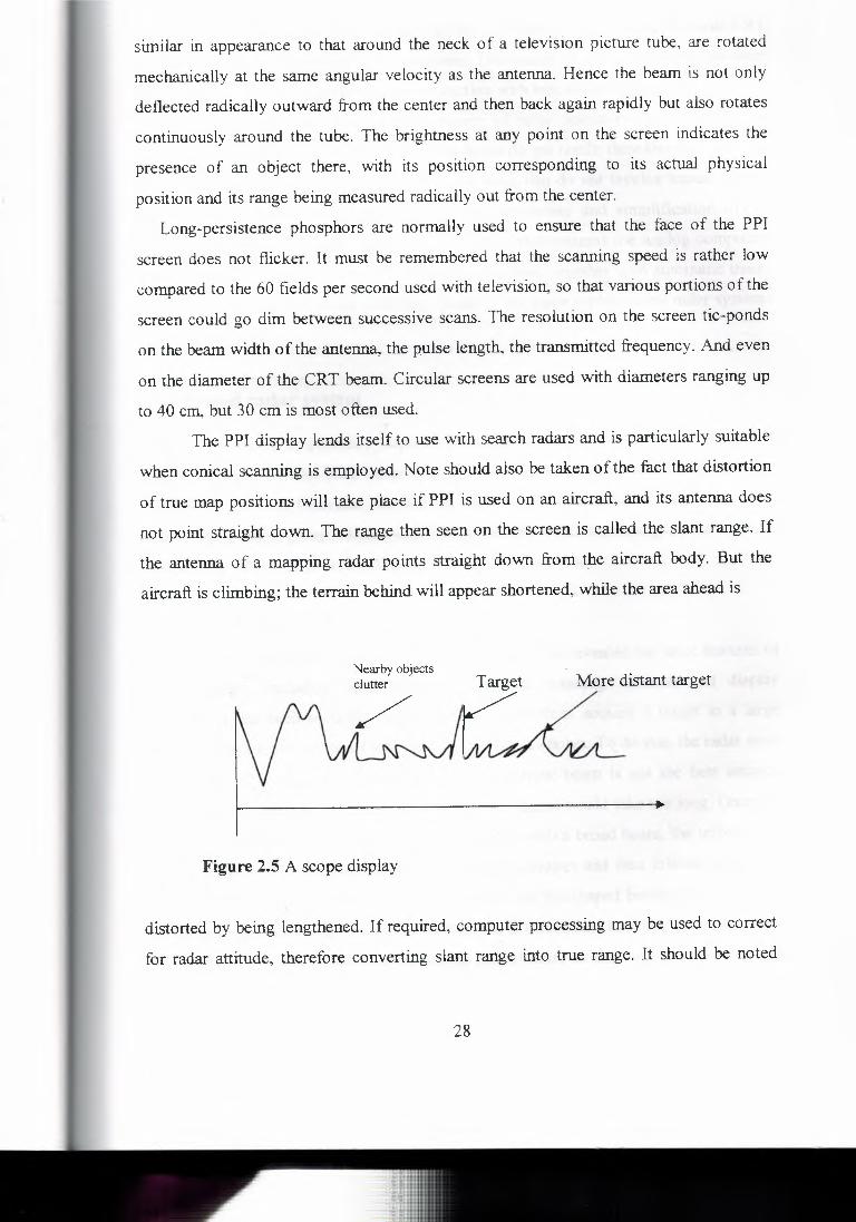
similar in appearance to that around the neck of a television picture tube, are rotated
mechanically at the same angular velocity as the antenna Hence the beam is not only
deflected radically outward from the center and then back again rapidly but also rotates
continuously around the tube. The brightness at any point on the screen indicates the
presence of an object there, with its position corresponding to its actual physical
position and its range being measured radically out from the center.
Long-persistence phosphors are normally used to ensure that the face of the PPI
screen does not flicker. It must be remembered that the scanning speed is rather low
compared to the 60 fields per second used with television, so that various portions of the
screen could go dim between successive scans. The resolution on the screen tic-ponds
on the beam width of the antenna, the pulse length, the transmitted frequency. And even
on the diameter of the CRT beam. Circular screens are used with diameters ranging up
to 40 cm, but 30 cm is most often used.
The PPI display lends itself to use with search radars and. is particularly suitable
when conical scanning is employed. Note should also be taken of the fact that distortion
of true map positions will take place if PPI is used on an aircraft, and its antenna does
not point straight down. The range then seen on the screen is called the slant range. If
the antenna of a. mapping radar points straight down from the aircraft body. But the
aircraft is climbing; the terrain behind will appear shortened, while the area ahead is
Nearby objects clutter Target More distant target
Figure 2.5 A scope display
distorted by being lengthened. If required, computer processing may be used to correct
for radar attitude, therefore converting slant range into true range. It should be noted
28

that the mechanics of generating the appropriate waveforms and scanning the radar CRT
are similar to those functions in TV receivers. Discussion of those, including the need
for saw tooth scanning waveforms, in conjunction with television receivers.
Automatic target detection the performance of radar operators may be erratic or
inaccurate (people staring at screens for long hours do get tired); therefore the output of
the radar receiver may be used in a number of ways that do not involve human opera
tors. One such system may involve computer processing and simplification of the
received data prior to display on the radar screen. Other systems use analog computers
for the reception and interpretation of the received data, together with automatic track
ing and gun laying ( or missile pointing). Some of the more sophisticated radar systems
are discussed later:
2.4 Pulsed radar system
A radar· system is generally required to perform one of two tasks: It must either
search for targets or else track them once they have been acquired. Sometimes the same
radar performs both functions, whereas in other installations separate radars are used.
Within each broad group, further subdivisions are possible, depending on the specific
application. The most common of these will now be described.
2.4.1 search radar·systems The general discussion of radar so far in this chapter has revealed the basic features of
search radars, including block diagrams, antenna scanning methods and display
systems. It has been seen that such a radar system must acquire a target in a large
volume of space, regardless of whether its presence is known. To do this, the radar must
be capable of scanning its region rapidly. The narrow beam is not the best antenna
pattern for this purpose, because scanning a given region would take too long. Once the
approximate position of a target has been obtained with a broad beam, the information
can be passed on to tracking radar, which quickly acquires and then fo Hows the target.
Another solution to the problem consists in using two fan-shaped beams (from a pair of
connected cut paraboloids,), oriented so that one is directional in azimuth and the other
in elevation. The two rotate together, using helical scan, so that while one searches in
29

azimuth, the other antenna acts as a height finder, and a large area is covered rapidly.
Perhaps the most common application of this type is the air-traffic-control radar used at
both military and civilian airports. If the area to be scanned is relatively small, a pencil beam and spiral scanning can
be used to advantage, together with a PPI display unit. Weather avoidance and airborne
navigation radars are two examples of this type. Marine navigation and ship-to-ship
radars are of a similar type, except that here the scan is simply horizontal, with a fan
shaped beam. Early-warning and aircraft surveillance radars are also acquisition radars
with a limited search region, but they differ from the other types in that they use UHF
wavelengths to reduce atmospheric and rain interference. They thus are characterized
not only by huge powers, but also by equally large antennas. The antennas are
stationary, so that scanning is achieved by moving-feedorsimilar methods.
2.4.1 Tracking Radar-Systems Once a target has been acquired, it may then be tracked, as discussed in the section
dealing with antennas and scanning. Tbe- most corrnmn tracking rretbod used purely for
tracking are the conical scan and monopulse systems described previously. A system that
gives the angular position of a target accurately is said to be tracking in angle. If range
information is also continuously obtained, tracking in range (as well as in angle) is said to
be taking place, while a tracker that continuously monitors the relative target velocity by
Doppler shift is said to be tracking in Doppler as well. If radar is used purely for tracking,
then search radar must be present also. Because the two together are obviously rather
bulky, they are often limited to ground or ship borne use and are employed for tracking
hostile aircraft and missiles. They may also be used for fire control, in which case
information is fed to a computer as well as being displayed. The computer directs the
antiaircraft batteries or missiles, keeping them pointed not at the target, but at the position
in space where the target will be intercepted by the dispatched salvo ( if all goes well)
some seconds later. Airborne tracking radars differ from those just described in that there is
usually not enough space for two radars, so that the one system must perform both
functions. One of the ways of doing this is to have a radar system, such as the World
War II SCR-584 radar, capable of being used in the search mode and then switched over to
30

the tracking mode, once a target has been acquired. The difficulty, however, is that the
antenna beam must be a compromise, to ensure rapid search on the one hand and
accurate tracking on the other. After the switchover to the tracking mode, no further
targets can be acquired, and the radar is "Blind" in all directions except one.
Track-while-scan (TWS) radar is a partial solution to the problem, especially if
the area to be searched is not too large, as often happens with airborne interception;
Here a small region is searched by using spiral scanning and PPI display. A pencil
beam can be used, since the targets arrive from a general direction that can be
predicted. The operator can mark blips on the face of the CRT, and thus the path of the
target can be reconstructed and even extrapolated, for use in fire control. The
advantage of this method, apart from its use. of only the one radar, is that it can acquire
some targets while tracking others, thus providing a good. deal of information
simultaneously. If this becomes too much for an operator, automatic computer
processing can be employed, as in the semiautomatic ground environment (SAGE)
system used for air defense. The disadvantage of the system, as compared with the pure
tracking radar, is hat although search is continuous, tracking is not, so that the accuracy
is less than that obtained with monopulse or conical scan.
Tracking of extraterrestrial objects, such as satellites or spacecraft, is another
specialized. form of tracking. Because the position of the target is usually predictable,
only the tracker is required .. The difficulty lies in the small size and great distance of
the targets. This does not necessarily apply to satellites in low orbits up to 600 km, but
certainly is true of _satellites in synchronous orbits 6,000 km up, and also of space
vehicles. Huge transmitting powers, extremely sensitive receivers and enormous fully
steer able antennas are required,
2.5 Moving· target indicator (MTI) It is possible to remove from the radar display the majority of clutter, that is,
echoes corresponding to stationary targets, showing only the moving targets. This is
often required, although of course not in such applications as radar used in mapping or
navigational applications. One of the methods of eliminating clutter is the use of MTI,
which employs the Doppler effect in its operation.
31

Doppler effect is the apparent frequency of electromagnetic or sound waves
depends on the relative radial motion of the source and the observer. If source and
observer are moving away from each other, the apparent frequency will decrease,
while if they are moving toward each other, the apparent frequency will increase. This
was postulated in 1842 by Christian Doppler and put on a firm mathematical basis by
Armand Fizeau in 1848. The Doppler effect is observable for light and is responsible
for the so-called red shift of the spectral lines from stellar objects moving away from
the solar system. It is equally noticeable for sound, being the cause of the change in
the pitch of a whistle from a passing train. It can also be used to advantage in several
forms of radar. Consider an observer· situated on a platform approaching a. fixed source of radiation,
with a.relative velocity +V,. A stationary observer would note.fr wave crests (or troughs)
per second if the transmitting frequency were J; Because the observer is moving toward
the source, that person of course encounters more than.fr crests per second. The number
observed under-these conditions is given by
(2.1)
Consequently,
J, ,_f,v, d - Ve
(2.2)
Where fr+ f ~ := anew observed frequency /d ·~ Doppler frequency difference
Note that the foregoing holds if the relative velocity, v,, is less than about 10
percent of the velocity of light. Ve, if the relative velocity is higher than that (most
unlikely in practical eases), relativistic effects must be taken into account, and a some
what more complex formula must be applied. The principle still holds under those
conditions, and it holds equally well if the observer is stationary and the source is in
motion. Equation (2.2) was calculated for a positive radial velocity, but if, v, is negative,
/' in Equation (2.2) merely acquires a negative sign. In radar involving a moving target,
the signal undergoes the Doppler shift when impinging upon the target. This target
becomes the "source' of the reflected waves, so that we now have a moving source and
32

a stationary observer (the radar receiver). The two are still approaching each other, and
so the Doppler effect is encountered a second. time, and the overall effect is thus double.
Hence the Doppler frequency for radar is
fd = 2 J: = 2 J; V r = 2 V r V C A.
(2.3)
Since!, Iv c = 1 I ,,1. where ).is the transmitted wave length.
The same magnitude of Doppler shift is observed regardless of whether a target is
moving toward the radar or away from it. With a given velocity. However, it will
represent an increase in frequency in the former case and a reduction in the latter. Note
also that the Doppler effect is observed only for radial motion, not for tangential
motion. Thus no Doppler effect will be noticed if a target moves across the field of view
of radar. However a Doppler shift will be apparent if the target is rotating, and the
resolution of the radar is sufficient to distinguish its leading edge from its trailing edge.
One example where this has been employed is the measurement of the rotation of the
planet Venus (whose rotation cannot be observed by optical telescope because of the
very dense cloud cover). On the basis of this frequency change, it is possible to determine the. relative
velocity of the target, with either pulsed or CW radar, as will be shown. One can also
distinguish between stationary and moving targets and eliminate the blips due to sta
tionary targets. This may be done with pulsed radar by using moving-target indication.
2.5.2 Fundamentals Of MTI Basically, the moving-target indicator system compares a set of received echoes
with those received during the previous sweep. Those echoes whose phase has remained
constant are then canceled out. This applies to echoes due to stationary objects, but
those due to moving targets do show a phase change; they are thus not canceled, nor are
noise, for obvious reasons. The fact that clutter due to stationary targets is removed
makes it much easier to determine which targets are moving and reduces the time taken
by an operator to "take in" the display. It also allows the detection of moving targets
whose echoes are hundreds of times smaller than those of nearby stationary targets and
which would otherwise have been completely masked. MTT can be used with a radar
33

using a power oscillator (magnetron) output, but it is easier with one whose output tube
is a power amplifier, only the latter will be considered here.
The transmitted frequency in the MTI system of Figure 2- 7 is the sum of the outputs of
two oscillators, produced in mixer 2. The first is the stalo, or stable local oscillator (note
that a good case can be made for using a varactor chain here). The second is the coho, or
coherent oscillator, operating at the same frequency as the intermediate frequency and
providing the coherent signal, which is used as will be explained. Mixers 1 and 2 are
identical, and both use the same local oscillator (the stab); thus phase relations
1) .\ )OT)e
Duplexer Klystron .
LY ~ amplifier
t fo+fe Modulator
'" Mixer l - ~ Mixer 2 - i ~
Stalo
1 •
f.
IF amplifier i Coho
J. r 1 Phase- -
sensitive ~ ne,tf"Mnr
- Amplifier I .
Delay line - Amplifier 2 - Sub tractor T=l/PRF
--,,
,r
MTI video out to
F . 2 7 Bl k ct· fMTI radar . lifi indicator igure . oc iagram o · usmg power amp 1 er output
34

existing in their inputs are preserved in their outputs. This makes It possible to use the
Doppler shift at the IF, instead of the less convenient radio frequency Jo+fe. The output
of the IF amplifier and a reference signal from the echo are fed to the phase-sensitive
detector; a circuit very similar to the phase discriminator.
The coho is used for the generation of the RF signal, as well as for reference in
the phase detector. And the mixers do not introduce differing phase shifts. The trans
mitted and reference signals are locked in phase and are said to be coherent; hence the
name of the coho. Since the output of this detector is phase sensitive, an output will be
obtained for all fixed or moving targets. The phase difference between the transmitted
and received signals will be constant for fixed targets, whereas it will vary for moving
targets. This variation for moving targets is due to the Doppler frequency shift, which is
naturally accompanied by a phase shift, but this shift is not constant if the target has a
radial component of velocity. If the Doppler frequency is 2000 Hz and. the return time
for a pulse is 124 µs ( 10 nmi), the phase difference between the transmitted and
received signals will be some value <I> (the same as for stationary target at that point)
plus 2000/124- =16.12complete cycles, or 16.12 *2'.lt"= 101.4-rad. When the next pulse
is returned from the moving target, the latter will now be closer, perhaps only 123 µs
away, giving a phase shift of 101.4- x 123/ 124 = 100. 7 rad. The phase shift is definitely
not constant for moving targets. The situation is illustrated graphically, for a number of
- successive pulses, Figure 2.8
• .,-
•••
"':' ·~ ,.
... . ..,
Mo~get· Figure .-8 operation of Mn radar ,(a),(b),(c) phase detector output for three
successive pulses; (d) sub tractoroutput.
35

It is seen from Figure 2-8 that those returns of each pulse that correspond to
stationary targets are identical with each pulse, but those portions corresponding to
moving targets keep changing in phase. It is thus possible to subtract the output for each
pulse from the preceding one, by delaying the earlier output by a time equal to the pulse
interval, or l /PRF. Since the delay line also attenuates heavily and since signals must be
of the same amplitude if permanent echoes are to cancel, an amplifier follows the delay
line. To ensure that this does not introduce a spurious phase shift, an amplifier is placed
in the undelayed line, which has exactly the same response characteristics (but a much
lower gain) than amplifier 1. The delayed and undelayed signals are compared in the
sub tractor (adder with one input polarity reversed), whose output is shown in Figure 2-
8d. This can now be rectified and displayed in the usual manner.
2.5.3 other-analog MTI system
These include area MTI, which involves subtracting a complete scan from the
previous one and displaying only the difference; it is done with storage CRTs. Another
system is almost identical. to the one described but uses a pulsed magnetron oscillator
instead of an amplifier. A different technique must be employed here to achieve
coherence, because each cycle of the· magnetron oscillations begins with a phase quite
unrelated to the previous pulsed cycle. Noncoherent MTI is also sometimes used,
deriving the required phase variations by comparing the returns from stationary and
radially moving targets. This method suffers from the disadvantage of requiring
stationary targets in each scan in addition to the moving target. Note that all coherent
systems require a fairly high pulse repetition frequency to ensure the return of several
pulses from each target. This also describes airborne moving-target indicator (AMTI), in
which compensation for the motion of the radar set is an added requirement.
2.5.4 delay lines Delay lines Because of the delay times required, it would be unthinkable to use
electromagnetic delay means in MTI. If the PRF is 1000, then the delay required is I ms,
in which time an electromagnetic wave in an air-dielectric line travels 300 km! The
method adopted to provide the requisite delay in practice is rather similar to that used
36

with mechanical filters. The signal is converted into acoustic vibrations, passed through
a mechanical resonant circuit and converted into an electrical signal at the output end,
with a suitable transducer. The most commonly used material for the delay line is fused
quartz, in which the velocity of sound is 5.44 m/ms.
Since this is still quite large (though manageable), the line can be folded. This
consists in having a many-sided prism, in which the acoustic waves are reflected from
the planesides. The signal then emerges 1 µs later if the total length of the folded path is
5.44 m. The attenuation in such a line is in excess of 40 dB, and this explains the
amplifier accompanying the line on the block diagram of Figure 2.7.
2.5.5 Blind Speeds When showing how phase shift varies if the target has relative motion,. a fictitious
situation, which gave a phase difference of 101.4 - 100.7 = 0.7 rad between successive pulses on the target was described in a previous section. If the target happens to have a
velocity whose radial component results in a phase difference of exactly 2rr rad between
successive pulses, this is the same as having no phase shift at all. The target thus
appears stationary, and. echoes from it are canceled by the MTI action. A radial velocity
corresponding to this situation is known as a blind speed, as are any integral multiples
of it. It is readily seen that if a target moves a half-wavelength between successive
pulses, the· change in phase shill will be precisely 21r rad.
We may state that
nJ.. vb =PRF-
2 (-2.3)
Where vb=blind speed
";.,= wavelength of transm.itted signal
n= any integer (include 0)
The fact that blind speeds exist need not be a serious problem and does not
normally persist beyond a small number of successive pulses. A target flying directly
toward the radar set at a constant velocity could cause this, but it would be sheer
coincidence, and a far-fetched one at that, for a target to do this accidentally. We do live
37

in a world that produces sophisticated electronic countermeasures, and it is not beyond
the realm of possibility that a target may be flying at a blind speed on purpose. A
wideband receiver and microprocessor on board the target aircraft or missile could
analyze the transmitted frequency and PRF and adjust radial velocity accordingly. The
solution to that problem is to have a variable PRF. That presents no difficulty, but
varying the delay in the MTI radar does. Having two delay lines and compensating
amplifiers can do it. One of these can be a small delay line, having a delay that is l 0
percent of the main delay, This second line will then be switched in and out on alternate
pulses, changing the blind speed by l O percent each time.
2.5.6 Digital MTI Is possible to replace the delay line and. amplifier arrangement of an analog MTI
system with digital-to-analog conversion of the received signal. After the signal has
been digitally coded, it can be stored in a computer memory. The echoes received. from
each pulse are now subtracted in the memory from those received from the previous
pulse, whereupon the difference is converted to analog form and displayed as before.
With digital MTI (or DMTI). No-difficulties arise in varying the PRF. It may be varied
almost randomly from one pulse to the next. Interestingly enough, the resolution limit in
DMTI is governed, in part, by quantizing noise. Just like in pcm., analog signals must be
quantized before their conversion to digital form.
2.6 Radar Beacons Is a small radar set consisting of a receiver, a separate transmitter and an antenna
which is often omni directional- When another radar transmits a coded set of pulses at
the beacon, i.e., interrogates it, the beacon responds by sending back its specific pulse
code. The pulses from the beacon, or transponder as it is often called, may be at the
same frequency as those from the interrogating radar, in which case the main station
together with its echo pulses receives them. They may alternatively be at a special
beacon frequency, in which case the interrogating radar requires a separate receiver.
Note that the beacon does not transmit pulses continuously in the same way as a search
or tracking radar but only responds to the correct interrogation.
38

One of the functions of a beacon may be to identify itself. The beacon may be
installed on a target, such as an aircraft, and will transmit a specific pulse code when
interrogated. These pulses then appear on the PPI of the interrogating radar and inform
it of the identity of the target. The system is in use in airport traffic control and also for
military purposes, where it is called identification, friend or foe (IFF).
Another use of radar beacons is rather similar. to that of lighthouses, except that ,
radar beacons can operate over much larger distances. An aircraft or ship, having
interrogated a number of beacons of whose exact locations it may be unaware ( on
account of being slightly lost), can calculate its position from the coded replies accu-
rately and automatically. The presence of a beacon on a target increases enormously the distance over
which a target may be tracked. Such active tracking gives much greater range than the
passive tracking so far described, because the power transmitted by the beacon (modest
though it normally is) is far in excess of the power that.this target would. have reflected
had it not carried a beacon .. This is best demonstrated quantitatively, as in the next
section. Beacon range equation following the reasoning used to derive the general radar range
equation;
ApT~T~B
4nr.2 (2.4)
Where all symbols have their previously defined meanings, except that the subscript T
is now used for quantities pertaining to the transmitter of the main radar, and B is used
for the beacon functions. Ao8 is the capture area of the beacon's antenna.
If P min, s is the minimum power receivable by the beacon, the maximum range for the
interrogation link will be:
(2.5) r = max,/
Substituting into Equation (2.4) for the power gain of the transmitter antenna
from Equation (2.5), and for the minimum power receivable by the beacon from
equation (2.6), and then canceling, we obtain the final form of the maximum range for
39

the interrogation link that is
r = max.I ApTptTAOB
,1. 2 kT/jf(F8 -1) (2.6)
It has been assumed in equation (2.6) that the bandwidth and antenna temperature
of the beacon are the same as those of the main radar. By an almost identical process of
reasoning, the maximum range of the reply link is
r - max,R - ApT~TAOB
,{ 2 kTi>f(FT -1)
(2.7)
Antenna is also tripled, A foldout, metallized umbrella spacecraft antenna with a
3-m (10-ft) diameter is certainly feasible. Again, the 13-dB noise figure for the beacon
receiver is conservative, and reducing it to 10 dB (still fairly conservative) would
further increase the range. A slower PRF and less insistence on pulses with steep sides
would permit a tenfold bandwidth reduction and a similar·pulse power-increase from the
beacon. A totaLrange for the reply link could comfortably exceed 1 OOOmillion Km, even
allowing forthe degradations mentioned above. That distance puts within all the planets
up to and including Saturn.
40

CHAPTER THREE
OTHER RADAR SYSTEMS
A number of radar systems are sufficiently unlike those treated so far to be dealt
separately. They include first of all CW radar which makes extensive use Doppler effect
for target speed measurements. Another type of CW radar is modulated to provide range
as well as velocity. Finally, phased array and planer array radars will be discussed in
this "separate" category. Here, the transmitted (and receiving) beam is steered not by
moving an antenna but by changing the phase relationship in the feeds for a vast array
of small individual antennas. These systems will described in tum.
3.1 CW Doppler radar
A simple Doppler radar, such as the one shown in figure 3.1, sends out
continuous sine. wave rather than pulses. It uses the Doppler effect to detect the
frequency change caused by a moving target and displays this as a relative velocity.
Since transmission here is continuous, the circulator of figure 3-1 is used to
provide insulation between the transmitter- and the receiver. Since transmission is
continuous, it would be pointless to use duplexer. The insulation of a. typical circulator
lS
Ci-cuator
cw trar 1S1111iter oscMor r. £,
EJ~ At.do HF==I ~
Figure 3.1 Simple Doppler CW Radar of the order of 30 dB, so that some of the transmitted signal leaks into the receiver. The
signal can be mixed in the detector with returns from the target, and the difference is the
Doppler frequency. Being generally in the audio range in most Doppler applications, the
detector output can be amplified with an audio amplifier before being applied to a
frequency counter. The counter is a normal one, except that its output is shown as
41
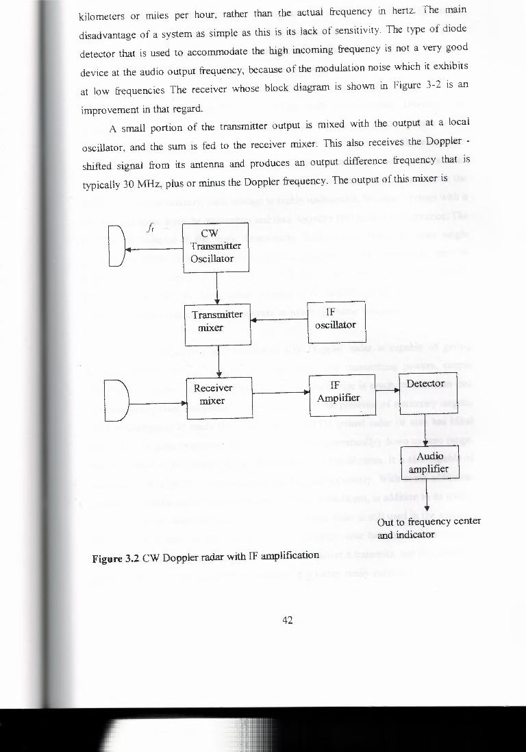
kilometers or miles per hour, rather than the actual frequency in hertz. The main
disadvantage of a system as simple as this is its lack of sensitivity. The type of diode
detector that is used to accommodate the high incoming frequency is not a very good
device at the audio output frequency, because of the modulation noise which it exhibits
at low frequencies The receiver whose block diagram is shown in Figure 3-2 is an
improvement in that regard. A small portion of the transmitter output is mixed with the output at a local
oscillator, and the sum is fed to the receiver mixer: This also receives the Doppler -
shifted signal from its antenna and produces an output difference frequency that is
typically 30 MHz, plus or minus the Doppler frequency. The output of this mixer is
n J; - CW .. Transmitter ..•
J Oscillator
, Transmitter _ IF rrnxer oscillator
, n Receiver - IF ~ Detector ,
Amplifier ~ rrnxer
,, Audio
amplifier
,, Out to frequency center and indicator
Figure 3.2 CW Doppler radar with IF amplification
42

amplified and demodulated again, and the signal from the second detector Is Just the
Doppler frequency. Its sign is lost, so that it is not possible to tell whether the target is
approaching or receding. The overall receiver system is rather similar to the super
heterodyne. Extra sensitivity is provided by the lowered noise, because the output of the
diode mixer is now in the vicinity of 30 MHz, at which FM noise has disappeared.
Separate receiving and transmitting antennas have been shown, although this
arrangement is not compulsory. A circulator could he used, as in the simpler set of
Figure 3-1. Separate antennas are used to increase the isolation between the transmitter
and receiver sections of the radar, especially since there is no longer any need or a small
portion of the transmitter output to leak into the. receiver mixer, as there was in the
simpler set. To the contrary, such leakage is highly undesirable, because it brings with it
the hum and noise from the transmitter ancL thus degrades the receiver performance. The
problem of isolation is the main determining factor, rather than any other single
consideration in the limiting of the transmitter output power. As a.consequence, the CW
power from such radar seldom exceeds 100 W and is often very much less. Gunn or
IMPATT diodes or, for the highest powers. CW rnagnetrons are used as power
oscillators in the transmitter. They operate at much the same frequencies as in pulsed
radar. Advantages, applications and limitations CW Doppler radar is capable of giving
accurate measurements of relative velocities, using low transmitting powers, simple
circuitry, low power consumption ancL equipment whose size is much smaller than that
of comparable pulsed equipment. It is unaffected by !he presence of stationary targets,
which it disregards in much the same manner as MTI pulsed radar (it also has blind
speeds, for the same reason as MTI). It can operate (theoretically) down to zero range.
Because, unlike in the pulsed system, the receiver is ON at all times. It is also capable of
measuring a large range of target speeds quickly and accurately. With some additional
circuitry. CW radar can even measure the direction of the target, in addition to its speed.
Before the reader begins to wonder why pulsed radar is still used in the majority
of equipment, it must be pointed out that CW Doppler radar has some disadvantages
also. In the first place, it is limited in the maximum power it transmits, and this naturally
places a limit on its maximum range. Second, it is rather easily confused- the presence
43

of a large number of targets (although it is capable of dealing with than one if special
filters are included). Einally (and this is its greatest drawback), Doppler radar is
incapable of indicating the range of the target. It can only show its velocity, because the
transmitted signal is unmodulated. The receiver cannot sense with a particular cycle of
oscillations is being received at the moment, and therefore cannot tell how long ago this
particular cycle was transmitted, so that range cannot be measured.
As a result of its characteristics and despite its limitations, the CW -radar system
has quite a number of applications. One of these is in aircraft navigation for· speed
measurement, Another application is in a rate-of-climb meter for vertical takeoff
planes., such as the. "Harrier,' which in 1969 became the first jet ever to on Manhattan
Island. in New York City. Finally, perhaps its most commonly encountered application is in the radar speed meters used by po lice.
l j l j ·~ ...
Mixer cw Frequency - - ...• Transm itter - modulator oscillator
i Amplifier Sawtooth
generator
Limiter - Frequency - Indicator . counter
Figure 3.3 Block diagram of simple FM CW radar altimeter.
3.2 Frequency-modulated CW radar
The greatest limitation of Doppler radar, i.e., its inability to measure range, may be
overcome if the transmitted carrier is frequency-modulated. If this is done, it should be
44

possible to eliminate the main difficulty with CW radar in this respect, namely, its
inability to distinguish one cycle from another. Using FM will require an increase in the
bandwidth of the system, and once again it is seen that a bandwidth increase in a system
is required if more information is to be conveyed (in this case, information with regard
to range).
Figure (3.3) shows the block diagram of a common application of the FM CW radar
system, the airborne altimeter. Sawtooth frequency modulation is used for simplicity,
although in theory any modulating waveform might be adequate. If the target (in this
case, the Earth) is stationary with respect to the plane, a frequency difference
proportional to the height of the plane will exist between the received and the transmit
ted signals. It is due to the fact that the signal now being received was sent at a time
when the instantaneous frequency was different. If the rate of change of frequency with
time due to the FM process is known, the. time difference between the sent and received.
signals may he readily calculated, as can the height of the aircraft. The output of the.
mixer in Figure (3.3), which produces the frequency difference, can be amplified, fed to
a frequency counter and then to an indicatorwhose output is calibrated in meters or feet.
If the relative velocity of the radar and the target is not zero, another frequency
difference, or beat, will superimpose itself on top of the frequency difference just
discussed, because of the Doppler frequency shift. However, the average frequency
difference will be constant and due to the time difference between the sending and
return of a particular cycle of the signal. Thus correct height measurements can still be
made on the basis of the average frequency· difference. The beat superimposed on this
difference can now be used, as with ordinary Doppler radar, to measure the velocity of
(in this case) the aircraft, when due allowance has been made for the slant range.
Tue altimeter is a major application of FM CW radar. It is used in preference to
pulsed radar because of the short ranges (i.e., heights) involved, since CW radar has no
limit on the minimum range. Whereas pulsed radar does have such a limit. Fatly simple
low-power equipment can be used, as with CW Doppler radar. Because of the size and
proximity of the Earth. Small antennas can also be used, reducing the bulk of the
equipment even further. A typical altimeter operates in the C band, uses a transmitter
power typically from 1 to 2 W, easily obtained from an IMP A TT or a Goon diode, and
45
has it range of up to 10.000 m or more, with a corresponding accuracy of about 5
percent.
3.3 phased array radars With some notable exceptions, the vast majority of radars have to cover an area in
searching and/or tracking, rather than always being pointed in the same direction. This
implies that the antenna will have to move, although it was seen that some limited. beam
movement can be produced by multiple feeds or by a moving feed antenna.. As lone as
antenna motion is involved. in moving the beam, limitations caused by inertia will
always exist, A limit on the maximum scanning speed will be imposed by antenna
mechanics.
The problem encountered with a. single antenna of fixed. shape is that the shape
of the beam it produces is also constant, unless some. rather complex modifications are
introduced. There is the difficulty caused by the fact that a single antenna can point in
only one direction at a time. Therefore sending out only one beam at a time. This makes
it rather difficult to track a large number of targets simultaneously and accurately. A
similar difficulty is encountered when trying to track some targets while. acquiring
others. Such problems could be overcom~, and a very significant improvement in
versatility would result, if a stationary antenna could produce a moving beam .. Although
this cannot be done readily with a single antenna, it can be done with an any consisting
of a large number of individual radiators. Beam steering can be achieved by the
introduction of variable phase differences in the individual antenna feeders, and
electronic variation of the phase shifts.
It will be recalled that the direction of the beam will be at right angles to the plane of
the array if all the dipoles are fed in phase, whereas feeding them with a progressive
phase difference results in a beam that is in the plane of the array, along the line joining
the dipole centers. It will thus be appreciated that if the phase differences between the
dipole feeds are varied between these two extremes, the direction of the beam will also
change accordingly. Extending this principle one step farther, it can be appreciated that
a plane dipole array. With variable phase shift to the feeders, will permit moving the
direction of the radiated beam in a plane rather than a line. Nor do the. individual
46

radiators have to be dipoles. Slots in wave-guides and other, arrangements of small
omni directional antennas will do as well. It is possible to arrange four such antenna
"" arrays, obtaining a full hemispherical coverage.
Each plane array would, for hemispherical coverage, point 45° upward. The beam
issuing from each face would have to move ±45° in elevation and ±45° in azimuth in
order to cover its quadrant. In practical systems. Vast numbers of individual radiators
are involved. One tactical radar has, in fact 4096 (i2) radiating slats per face. Types There are broadly two different types of phased arrays possible. In the first, one
high-power tube feeds the whole array; the array is split into a small number of
subarrays, and a separate tube feeds each of these. The feeding is done through high
level power dividers (hybrids) and high-power phase shifters. The phase shifters are
often ferrite. Indeed, IJ).Ost of the advances in ferrite technology in the 1960s were spin
offs from phased. array military contracts. It will be recalled that the phase shill
introduced by a suitable piece of ferrite depends on the magnetic field to which the
ferrite is subjected; this is by adjusting this magnetic field, a full 360° phase change is
possible.
Digital phase shifters are also available, using PIN diodes in distributed circuits.
A particular section will give a phase shift that has either of two values, depending· on
whether the diode is ON or OFF. A typical "4-bit" digital phase shifter may consist of
four PIN phase shifters in series. The first will produce a shift of either O or 22Yi°,
depending on the diode bias. The second offers the alternatives of O or 45°, the third. 0 or
90° and the fourth O or 180°. By using various combinations, a phase shift anywhere
between O and360° (in 22Yi° steps) may be provided. The ferrite phase shifters have the
advantages of continuous phase shift variation and the ability to handle higher powers.
PIN diode phase shifters, although they cannot handle quite such high powers, are able
to provide much faster variations in phase shill and therefore beam movement. As a
good guide, the phase variations that take a few milliseconds with ferrite shifters (Figure
3-4) can be accomplished in the same number of microseconds with digital shifters.
A second broad type of phased array radar uses many RF generators, each of
which drives a single radiating element or bank of radiating elements. Semiconductor
47
diode generators are normally used, with phase relationships closely controlled by
means of phase shifters, The use of YTG and microwave integrated circuit (MIC) phase.
shifters has enhanced several aspects of the phased array radar: The YTG phase shifter,
when coupled with irises for matching purposes, results in a radiating element which is
compact, easy to assemble and relatively inexpensive. The MIC phase shifter greatly
reduces the size of arrays, since it is itself small and integrated into the radiating
element.
These multi generator arrays provide wide-angle scanning over an appreciable.
frequency range. Scanning may be accomplished through a combination of mechanical
and electronic means, or-through electronic means alone. The array shown in Figure 3-6
employs RF generators to drive each horizontal bank of radiators. Elevation scanning
can therefore be ~ccomplished electronically, although horizontal scanning uses
traditional mechanical techniques. The array shown in Figure 3-6 provides one
generator for each radiating element, and this makes electronic scanning for both
horizontal and vertical planes possible, although the cost for this type of away is of
course significantly higher. The number of phases /generator elements increases from
70 fora typical array of the first type to 4900 for an array of the second type.
Arrays using multiple semiconductor diode generators have several advantages .. The
generators operate at much lower power levels and are therefore cheaper and more
reliable, With so many independent RF generators, any failures that occur will be
individual rather than total, ~id their effect will thus be merely a gradual deterioration,
not a catastrophic failure. The disadvantages of the second system include. the high cost
of so many Gunn or IMPATT or even TRAPATT oscillators. The lower available
powers at higher frequencies are yet another problem; even 4096 oscillators producing
100-W pulses each give out only a little over 400 kW, much less than a medium-large
tube. The power dissipation is more of a problem than with tubes, since efficiencies of
diode RE generators are noticeably lower.
In a sense, phased array radars have been the "glamour " systems, in terms of
development money spent and space devoted in learned journals. Certainly, there is no
doubt that they can work and currently do so in quite a number of establishments. They
can be astonishingly versatile. For example, the one array can rapidly locate targets by
48
sending out two fan-shaped beams simultaneously. One is vertical and moves
horiz~tally, while the other is horizontal and moves vertically. Once a target has been
located, it can then be tracked with a narrow beam, while other wide beams meanwhile
acquire more targets. The phased array radar utilizing electronic techniques benefits
from inertia less scanning. Since the beam can be- redirected and reconfigured in
microseconds, one array can be programmed to direct pulses to various locations m
rapid. succession. The result is that the array can simultaneously undertake- acquisition
and tracking. operations for multiple targets. The possibilities are almost endless.
Because phased array radars have to perform complex tasks, they must themselves also
be complex. This makes them atrociously expensive. One authority quotes it typical cost
of $1 million for just the phase shifters and their drivers in one system, That still leaves
the computer control, RF sources, power dividers and the arrays themselves, as well as
the costs of testing and installation. A significant cost reduction could. he achieved by
mass production, if demand for phased array radars increases. It is to be hoped that this
situation does not develop into a. vicious circle.
Figure· 3A phased array antenna that provides for elevation scanning by feeding
each horizontal row of elements with a separate phase shifter.
Related technology Signal processing is one aspect of radar technology, which
has resulted in a significant improvement in radar capabilities. Signal processing
systems currently in use with radar systems depend heavily on computer and microchip
technology. These systems perform the functions of analyzing, evaluating and
displaying radar data, as well as controlling the subsequent pulse emissions.
49

f~· /;!l:
~ ignal processing used with radar systems includes filtering operations d}\Q. he 1 ,_, :.. :'f \ '-'' full bandwidth signal to separate signal waveforms from noise and interfering b;k- r.~ \:: . ,0 ground signals. This accommodation to the. electromagnetic environment in which th'i,-~E-~
radar system operates is further enhanced by the. ability to utilize computer algorithms to
alter pulse frequency and other characteristics, in response to the transmissions of other
systems. By varying the transmitted signals, it is possible for the system to attain
significant immunity from interference (from other signals). Computer evaluation and
control prevent interference to the system since the interfering signal cannot track the
frequency changes and the sub pulses generated by the. system at the direction of the
signal-processing computer. Usable images can be obtained even in adverse or very
active electromagnetic environments. This enhancement of the- radar system capability
is of particular· value to military and other systems, which must operate, in close
proximity to other radars. With sophisticated computer systems available to the radar,
additional display manipulations and improvements can be achieved.
Radar systems benefit from large-scale. integration in the same way as other
electronic fields. As a "signal processor on a chip" becomes a reality, the cost,
complexity and size of even a.complex radar system will decrease. Digital simulation of
analog filters and other devices will also contribute to reduction of system costs.
Because real-time radar signal processing. needs to execute instructions rates exceeding
2 * 10 7 operations per second, the current digital switching speed has become a limiting
factor. As digital technology improves in speed, signal processing will become even
more important for radar systems.
3.3.1 Planar Array Radars
The planar array radar uses a high-gain planar array antenna.. A fixed delay is estab
lished between horizontal arrays in the elevation plane .. As the frequency is changed, the
phase front across the aperture tends to tilt, with the result that the beam is moved in
elevation.
50

Antenna array
Transmitter
Fl F3 F4 F5
Five subpulses each at different frequency
Figure 3.5 frequency scanning as used by planar array radar· causes radars beam to be
elevated slightly above one another.
Figure 3-5 shows a. planar antenna array to which a burst of five sub pulses, each
at a different frequency, is applied. The differing frequencies cause each successive
beam to be elevated slightly more than the previous beam.
27-5° elevation
Antenna array
300 Km.range ~
Figure 3.6 planer array radar showing five separate groups of fine beams, which
permit scanning of27.5° of elevation.
51

The radar illustrated in figure 3-6 with five of the five beams groups used scans a 2.7.5°
ele.vation. The planner array system has several advantages in that each beam group has
full-transmitted peak power, full antenna gain and full side lobe, performance. The use
of frequency changes provides economical, simple and reliable inertia less elevation
scanning.
52

CHAPTER FOUR
4 . .1 Air Defence.
Historically, the military has played. the leading role in the use and development
of radar: The detection and interception of opposing military aircraft in air defence has
been the predominant military use of radar. The military also uses airborne radar to scan
largebattlefields for presence of enemy forces and equipment and to pick out precise targets for boms and missiles ..
A typical surface-based air defance system relies upon several radar systems.
First, a. lower frequency radar with a high-powered transmitter and a large anntena (
searches the airspace for all aircraft, both friend. and foe. A secondary radar system
reads the transponder signals sent by each aircraft to distinguish between allies and
enemies. After enemy aircraft are detected, operators track them more precisely by
using high-frequency waves from special fire control radar systems. The air· defence
system may attempt to shoot down threatening aircraft with gunfire or missiles, and
radar sometimes guides both gunfire and. missiles. Longer-range air defence. systems use .
missiles with internal guidance. These systems track a target using data. from a radar
system on the missiles .. Suen missile-borne radar· system are called seekers. The seeker
uses radar signals from the: missile. or radra signale from a transmitter on the ground to
determine the position of the target relative to the missile, and then passes the
information to the missiles guidance: system. The military uses surface-to-air systems
for defence against balistic missiles as well as aircraft .. During the Cold War both the
United States and the Union of Soviet Socialist Republics (USSR) did a great deal of
research into defence against intercontinental ballistic missiles (ICBMs) and submarine
launched ballistic missiles. The United states and the USSR sigmed the Anti-Ballistic.
Missile (ABM) treaty in l 972~ this treaty limited each of the superpower to a single,
limited capability system. The U.S. system consisted of a low-frequency (UHF) phased
array radar around the perimeter of the country, another phased-array radar to track
53
incoming missiles more accurately, and several very high-speed missiles to intercept the
incoming ballistic missiles. The second radar guided
The interceptor missiles. Airborne air defence system incorporate the same functions as
ground-based air defence, but special aircraft carry the large are search radar systems.
This is necessary because it is difficult for high-performance fighter aircraft to carry
both large radar system and weapons.
Madren warfare uses air-to-ground radar to detect targets on the ground and to
monitor the movement of the troops. Advanced Doppler techniques and synthetic
aperture radar have greatly increased the accuracy and usefulness of air-to-ground radar
since their introduction in the 1960s and 1970s. Military forces around the world use
air-to-ground radar for weapon aiming and for battelfield surveillance. The United
States used. the Joint Surveillance and Tracking Radar System (JST ARS) in the Persian
Gulf War (1991 ), demonstarting modem radar's abilty to provide information about
enemy troop concentrations and movements during the day or night, regardless of
weather conditions.
The military uses several techniques to attempt to avoid detection by enemy
radar. One common technique is jamming, that is, sending deceptive signals to the
enemy's radar system. During World War II (1939-1945), flyers under attack jammed
enemy radar by dropping a large clouds of chaff: small pieces of aluminum foil or some
other material that reflects radar well. "False" returns from chaff hid the aircraft's exact
location from enemy's air defense radar. Modem jamming uses sophisticated electronic
system that analyze enemy radar, and then send out false radar echoes that mask the
actual target echoes or deceive the radar about a target's location.
Stealth technology is a collection of methods that reduce the radar echoe sfrom
aircraft and other radar targets. Special paint can absorb radar signals and sharp angles
in the aircraft design can reflect radar signals in deceiving dirctions. improvements in
jamming and stealth technology force the contiual development of high-power
transmitters, antennas good at detecting weak signals, and very sensitive receivers, as
well as techniques for improved clutter rejection.
54

4.1.1 Radarin World War II
None of the early demonstrations of radar generated much enthusiasm. The
commercial and military value of radar did not become readily apparent until the mid
l 930s. Befor World War II, the United States, France, and the United Kingdom were all
carrying out radar reasearch. Begining in 1935, the British built a network of ground
based aircraft detection radar, called Chain Home, under the direction of Sir Robert
Watson-Watt. Chain Home was fully operational from 1938 until the end of World War
II in 1945 and was extremely instrumental in Britain's defence against Germen
bombers. The. British recognized the value of radar with frequency much higher than the
radio waves used for most syetms. A breakthrough in radar technology came in 1939 '
when two British scientists, physicist Henry Boot and biophysicist John Randall,
developed the resonant-cavity magnetron. This device generate high-frequency radio
pulses with a large amount of power, and. it made the development of microwive radar
possible. Also in 1939, the Massachuestts Institute of technology (MIT) Radiation
Laboratory was formed in Cambridge, Massachusetts, bring, together U.S. and British
radar research. in March 1942 scientists demonstrated the detection of ships from air.
This technology became the basis of anti ship and antisubmarine radar for the U.S.Navy
The U.S. Army operated air surveillance radar at the start of World War II. The
army also used early forms of radar to direct antiaircraft guns. initially the. radar systems
were used to aim searchlight so soldier aiming the gun could see where to fire, but the
system evolved into fire-control radar that aimed the guns automatically.
4.1.2 Radar during the Cold War
With the end of World War II, interest in radar development declind .. Some
expeiments continued, however; for instance, in 1946 the U.S. Army Signal Corps
bounced radar signals off of the moon, unshering in the field of radar astronomy. The
groeing hostility between the United States and the Union of Soviet Socialist Republics,
the so-called Cold War-renewed military interest in radar improvments.
55

After the Soviets detnoted their first atomic bomb in 1949, interest in radar
development, especially for iar defence, surged. Major programs included the
installation of the Distant Early Warning (DEW) network of long-range radar across the
northern reaches of North America to warn against bomber attacks. As the potential
threat of attack by ICBMs increased, the United Kingdom, Greenland, and Alaska
installed the Ballistic Missile Early Warning System (BMEWS).
4.2. Radar Systems Classification Methods
During World War II, each service used its own method to designate its
electronic radar/tracking systems. For example, Army radars were classified under the ,,-
initials SCR which stood for "Signal Corps Radio." Different designations for similar·
systems confused manufacturers and complicated electronics procurement. In February
1943, a universal classification system was implemented for all services to follow,
ending the confusion. To indicate that an electronic system designation followed the
new universal classification, the letters "AN," for Army-Navy, were placed ahead of a
three-letter code. The first letter of the three-letter code denoted the type of platform
hosting the electronic device, for example: A-Aircraft; C-Air transportable (letter no
longer used starting in thel9_50s); F-Fixed permanent land-based; G-General ground
use; M-Ground mobile; S-Ship-mounted; T-Ground transportable. The second letter
indicated the type of device, for example: P-Radar (pulsed); Q-Sonar; R--Radio. The
third letter indicated the function of the radar system device, for example: G-Fire
control; R-Receiving (passive detection); S-Search; T-Transrnitting. Thus an AN/FPS-
20 represented the twentieth design ofan Army-Navy "Fixed, Radar, Search" electronic
device.
4.2.1 World War II Radars
This section describes the World War II vintage radars that saw service during
the Cold War. The systems are listed in numerical order, bypassing the three-letter code.
During World War II, search and height-finder radars became components of America's
electronic arsenal. The function of the search radar was to detect and obtain a line of
56
bearing on an aircraft. Early models such as the SCR-270 and 271 looked like large bed
springs. Later designs, such as the AN/CPS-5 looked like a large oval dish. Search
radars generally rotated full circle around a central axis. In contrast to the rotating
search radar antenna, the horizontally mounted height-finder radar focused on the
tracked aircraft's reported bearing. The radar antenna dish then scanned up and down to
provide the operators with the estimated height of the aircraft.
4.2.1.1 AN/TPS-lB, lC, lD
Bell Telephone Laboratories developed this radar that subsequently was
produced by the Westem Electric Company. A crew of two could operate the radar. The
lB model could detect bombers at 10,000 feet at a distance of 120 nautical miles. The
height detection and range on the lC and ID models exceeded those of the lB. The
transmitter sent its pulse at an L-band frequency between 1220 to 1280 megahertz
(MHz). This long-range search radar was used in the temporary Lashup system
beginning in 1948.
4.2.1.2 AN/CPS-4
Developed by MIT's Radiation Laboratory, this height-finding radar was nicknamed
"Beaver Tail." The radar was designed to be used in conjunction with the SCR-270 and
SCR-271 search sets. The CPS-4 required six operators. This S-band radar, operating in
the 2700 to 2900 MHz range, could detect targets at a distance of ninety miles. The
vertical antenna was twenty feet high and five feet wide. This radar was often paired
with the AN/FPS-3 search radar during the early 1950s at permanent network radar
sites.
4.2.1.3 AN/CPS-5
Bell Telephone Laboratories and General Electric developed this search radar. General
Electric began producing sets in January 1945. Designated as a transportable medium
range search radar; the unit was ideal for use in the Lashup system in conjunction with
the ANrrPS- l O height-finder radar. It could be operated with a crew of ten. Some of
57

these units remained to serve in the first permanent network. Designed to provide a
solid search of up to 60 miles at 40,000 feet, the radar often had success tracking aircraft
as far as 210 miles away.
4.2.1.4 AN/CPS-6, 6A, 6B
The AN/CPS-6 was developed during the later stages of World War II by the Radiation
Laboratory at MJT. The first units were produced in mid-1945. General Electric
developed and produced the A-model and subsequent B-model at a plant in Syracuse,
New York. The unit consisted of two antennas. One of the antennas slanted at a forty
five degree angle to provide the height-finder capability. Initially, the radar was
designed. to detect fighter aircraft at 100 miles and.I 6,000 feet. The radar used five
transmitters that operated at S-band frequencies ranging from 2700 AN/CPS-6to 3019
MHz. It took twenty-five people to operate the radar. An AN/CPS-6 radar was installed
as part of the Lashup system at Twin Lights, New Jersey, in 1949 and proved capable of
detecting targets at ranges of eighty-four miles. The first units of the follow-on 6B radar
set were ready for installation by mid-1950. Fourteen 6B units were used within the first
permanent net-work. A component designed. to improve the radar's range was added in
1954. Initial tests showed the 6B unit had a range of 165 miles with an altitude limit of
45,000 feet .. One radar unit and its 'ancillary electronic equipment had to be transported
in eighty-five freight cars. The Air Force phased out the 6B model between mid-1957
and mid-1959.
4.2.1.5 ANffPS-10, lOA /AN/FPS-4
MIT's Radiation Laboratory developed and produced the first version of this radar near
the end of World War IL Zenith produced the A-model sets in the post-war period. The
vertically mounted antenna was three feet wide and ten feet long. Two operators were
needed to run the set. The initial model operated at a frequency of 9000 to 9160MHz
and had a maximum reliable range for bombers of 60 miles at 10,000 feet. An updated
version designated the AN/FPS-4 was produced by the Radio Corporation of America
(RCA) beginning in 1948. Some 450 copies of this and the trailer-mountedAN/MPS-8
version were built between 1948 and 1955.
58
4.2.2 Early Cold War Search Radars
Early Cold War search radars essentially were advanced or improved versions of World
War 11 era sets. In some cases, the performance of the new sets fell short of
expectations.
4.2.2.1 AN/FPS-3, 3A
The AN/FPS-3 was a modified version of the AN/CPS-5 long-range search radar. The
first units came off the Bendix production line and were. ready for installation in late
1950. Forry-eight of these L-band units were used within the first permanent network. <,
The AN/FPS-3B incorporated an AN/GPA-27, which increased the search altitude
to65,000 feet. Installation of these modifications began in 1957.
4.2.2.2 AN/FPS-5
The AN/FPS-S was a long-range search radar produced in the early 1950s by Hazel
tine. Deployment was limited.
4.2.2.3 AN/FPS-8
The AN/FPS-8 was a medium-range search radar operating on the L-band at a
frequency of 1280 to 1380 MHz. Developed in the 1950s by General Electric, over200
units of this radar were produced between 1954 and 1958. Variants of this radar
included theAN/GPS-3 and the AN/MPS-11.
4.2.2.4 AN/FPS-10
This unit was essentially a stripped down version of the AN/CPS-6B. Thirteen of these
units served within the first permanent network.
SAGE System Compatible Search Radars
Various manufacturers began design work on compatible search radars for SAGE
systems in the mid- l 950s in conjunction with the development of the SAGE Command
59

and Control System. Because Project LAMPLIGHT indicated radar vulnerability to
electronic countermeasures, the Air Force developed a series of radars that could shift
frequency. These frequency-diversity (FD) radars included the AN/FPS-24, Ai~/FPS-
27, andAN/FPS-35.
4.2.3 SAGE System Compatible. Search Radar
4.2.3.1 AN/FPS-7, 7A, 7B, 7CI 7D
In the mid-1950s, General Electric developed a radar with a search altitude of 100,000
feet and a range of 270 miles. This radar was significant in that it was the first stacked
beam radarto enter into production in the United States. Designed to operate in the L
band at 1250 to 1350 MHz, the radar deployed. in late 1959 and the early 1960s. The
AN/FPS-7 was used for both air defense and air traffic control in New York, Kansas
City, Houston, Spokane, San Antonio, and elsewhere. In the early 1960s, a modification
called AN/ECP-91 was installed to improve its electronic countermeasure (ECM)
capability. About thirty units were produced.
4.2.3.2 AN/FPS-20,20A, 20B
This Bendix-built radar was an AN/FPS-3 search radar with an AN/GP A-27
installed. Designed to operate in the L-band frequencies of 1250 to 1350 MHz, the radar
had a range of over 200 miles. By the late 1950s this radar dominated the United States
radar defense net. Deployment continued into the early 1960s. In June 1959, Bendix
received a contract to provide private industry's ivfK.-447 (the same as the military's
AN/GPA-103) and ivfK-448 (AN/GPA-102) anti-jam packages to the radars. With the
addition of these packages, the Air Force redesignated the radars. The AN/FPS-20A
with the AN/GP A-102 became the AN/FPS-66 and the AN/FPS-20A with the
AN/GP A-103 became the AN/FPS-67. Over 200 units were built.
4.2.3.3 AN/FPS-24
60

General Electric built an FD search radar designed to operate in the Very High
Frequency (VHF) at 214 to 236 MHz. There were problems with this radar at the test
site at Eufaula, Alabama, in 1960. These problems required many modifications.
Additional problems occurred when deployment was attempted in 1961. When the radar
finally deployed, bearing problems often occurred due to the eighty-five ton antenna
weight. Twelve systems were built between 1958 and 1962.
4.2.3.4 AN/IFPS-27 ,27 A
Westinghouse built an FD search radar designed to operate in the S-band at 2322
to2670 MHz.· The radar was designed to have a maximum range of 220 nautical miles
and search to an altitude of 150,000 feet. System problems required several
modifications at the test platform located at Crystal Springs, Mississippi .. Once these
problems were solved, the first of twenty units in the continental United States became
operational a. Charleston, Maine, in 1963. The last unit was installed at Bellefontaine,
Ohio, a year· later. In the early 1970s, AN/FPS-27 radar stations that bad not been
shutdown received a modification (solid state circuitry replacing vacuum tubes) that
improved reliability and saved on maintenance costs.
4.2.3.5 AN/FPS-28.
Raytheon designed this search radar to operate at 410 to 690 MHz. A test unit
was placed at Huoma Naval Air Station (NAS) in Louisiana.
4.2.3.6 AN/FPS-30
Bendix built this long-range search radar that operated in the L-band.
4.2.3.7 AN/FPS-31
Designed by Lincoln Laboratory; this huge radar was designed to be compatible
with the SAGE system A prototype was built at Jug Handle Hill in West Bath, Maine.
The antenna was 120 feet wide and 16 feet high. Operations began in October 1955.
After a period of unexpected clutter, it was determined that the radar received echoes
61

from the aurora borealis (Northern Lights) and this hindered tracking. Although this
model was never mass-produced for active use, lessons learned from this radar would
continue supporting SAGE system research and development.
4.2.3.8 AN/FPS-35
This Sperry-built FD long-range search radar was designed to operate at 420 to
450MHz. It was first deployed in December 1960, but problems hampered the program.
Four of these units were operational in 1962 .. The system suffered frequent bearing
problems as the antenna weighed seventy tons.
4.2.3.9 AN/FPS-64, 65, 66, 67~ 67 A, 72
These radars were modified versions of the Bendix AN/FPS-20 search radar. See
theANIFPS-20 entry.
4.2.3.10 AN/FPS-87 A
Bendix built this long-range L-band search radar that was based on the ANIFPS-20. See
the ANIFPS-20 entry.
4.2.3.11 AN/IFPS-88
General Electric produced this updated version of the AN/FPS-8 radar in the
latel960s. The AN/FPS-88 operated in the L-band at 1280 to 1380 MHz and featured
some ECM capability.
4.2.3.12 AN/IFPS-91
This radar was another version of the ANIFPS-20 search radar produced by
Bendix. See the AN/FPS-20 entry.
4.2.3.13 AN/IFPS-93
Raytheon modified the AN/FPS-20 radar to create this radar. See the ANIFPS-20entry.
62

4.2.3.14 AN /IFPS-100
This radar was another modernization of the Bendix AN/FPS-20 radar. See
theAN/FPS-20 entry.
4.2.3.15 AN/FPS-107
This Westinghouse-built search radar operated in the L-band at 1250 to 1350
MHz. SAGE System Compatible Height-finder Radars.To complement the search
radars, height-finding radars were developed to detect aircraft at increasing altitudes.
The AN/FPS-6 would serve as the standard model for much of the Cold War.
4.2.3.16 AN/IFPS-6,6A, 6B
The AN/FPS-6 radarwas introduced into service in the late 1950s and served as
the principal height-finder radar for the United States for several decades there after.
Built by General Electric, the S-band radar radiated at a frequency of 2700 to 2900
MHz. Between 1953 and 1960, 450 units of the AN/FPS-6 and the mobile ANIMPS-14
version were produced.
4.2.3.1 T AN/FPS--26
Avco Corporation built this height-finder radar that operated at a frequency of 5400 to
5900 MHz. This radar deployed in the 1960s.
4.2.3.18 AN/FPS-89
General Electric produced this improved version of the AN/FPS-6 height-finder radar in
the early
1970s. Operating in the S-band, this high-power radar was capable of detecting targets
at a. range of over 110 miles.
63

4.2.3. l 9 AN/FPS-90
Martin Marietta produced the high-powered version of the AN/FPS-6 height-finder
radar. Seethe ANIFPS-6 entry.
4.2.3.20 AN/FPS-116
This radar was another modernized version of the ANAFPS-6 height-finder radar.
, Seethe AN/FPS-6 entry.
4.2.3.21 Gap-Filler Radars
Gap-filler radars were designed to cover areas where enemy aircraft could fly low
enough to evade detection by distant long-range search radars. Between 1957 and 1962,
some 200 AN/FPS-14- and AN/FPS-18 models were built.
4.2.3.22-AN /FPS-14
This medium-range search radar· was designed and built by Bendix as a SAGE system
gap-filler radar to provide low-altitude coverage. Operating in the S-band at a frequency
between 2700 and 2900 MHz; the AN/FPS-14 could detect at a range of 65 miles. The
system was deployed in the late 1950s and 1960s.
4.2.3.23 AN/FPS-18
This medium-range search radar was designed and built by Bendix as a SAGE system
gap-filler to provide low-altitude coverage. The radar operated in the S-band at a
frequency between 2700 and 2900 MHz. The system deployed in the late 1950s and
1960s.
4.2.3.24 AN/FPS-19
This Raytheon gap-filler radar was deployed on the Distant Early Warning (DEW)Line.
It operated in the S-band.
64-

4.2.4 North Warning System Radars
The North Warning System replaced the DEW Line system in the late 1970s. New
equipment came with the change in system designation. A key component of the
modernization was a long-range radar system formally known as Seek Igloo. The
system is based around the AN/FPS-117.
4.2.4.1 AN/FPS-117
This 3-D long-range radar was built by GE Aerospace for use at Alaskan sites and on
the. Northern Warning System. The radar operated at 1215 to 1400 MHz and had a range
of about 220 miles ..
4.2.4.2 AN/FPS-124
This medium-range radar was built by Unisys to serve as an unmanned gap-filler radar
on the North Warning System.
Ballistic Missile Early Warning System (BMEWS) Radars
With the advent of ballistic missiles, millions of dollars were spent to research, develop,
test, and deploy BMEWS radars.
4.2.4.3 AN/FSS-7
This radar was a modified AN/FPS-26 height-finder radar produced by Avco
Corporation to detect submarine-launched ballistic missiles. The system deployed at
seven sites in the 1970s. Six sites were phased out during the early 1980s. The remaining
unit continued in operation in the southeast for a few more years to provide coverage
over Cuba.
4.2.4.4 AN /FPS-17
65

With the Soviet Union apparently making rapid progress in its rocket pro gram, inl 954
the United States began a program to develop a tracking radar. General Electric was the
contractor and Lincoln Laboratory was the subcontractor. This tracking radar, the
AN/FPS-1 7, was conceived, designed, built, and installed. for operation in less than two
years. Installed at Laredo AFB in Texas, the first AN/FPS--17 was used to track rockets
launched from White Sands, New Mexico. The radar was unique; it featured a fixed
fence antenna that stood 175 feet high and 110 feet wide. The transmitter sent out ash
pulse at a frequency between 180 to 220 MHz. Units were installed in the late.I 950s at
Shemya Island in the Aleutians and in Turkey. The unit at Shemya subsequently was
replaced by the Cobra Dane (AN/FPS-100) radar.
4.2.4.5 AN/FPS-49,49A
This large radar was built by RCA for use in the BMEWS program and the satellite
tracking program that deployed in the 1960s. The prototype unit operated at
Moorestown, New Jersey. Two additional units were installed in Greenland and
England. The radar frequency operated in the Ultra High Frequency (UHF) band and
could track objects beyond 3,000 miles.
4.2.4.6 AN/FPS-50
This was a BMEWS program surveillance radar that used a large, fixed-antenna fence
system. Two beams were projected from the antenna array. Objects passing through the.
lower-angled beam provided initial data and warning for the North American Air
Defense Command (NORAD). Data produced when the object passed through the upper
beam allowed computation of trajectories on launch and target points. The radar
operated in the UHF range at 425 MHz. General Electric, Heavy Military Electronics
Department, installed these systems at Clear, Alaska, and Thule, Greenland, during the
earlyl 960s.
4.2.4. 7 AN/FPS-85
66

This UHF, 3-D, phased-array radar was designed by Bendix for satellite tracking. Built
in the ear-ly 1960s at Eglin AFB in Florida, it was the first phased-array unit in the
United States. A fire destroyed the first model in 1965. A rebuilt model became
operational in 1969. The southward-sloped structure contained a square transmitter face
placed alongside a larger octangular receiving face. The transmitter operated at a UHF
frequency of 442. MHz. The .A.N/FPS-85 was also used to detect submarine-launched
ballistic missiles.
4.2.3.8 AN/FPS-92
This improved version of the AN/FPS-49 tracking radar was used in the BMEWS
Program. Built by RCA, this radar was installed at Clear; Alaska, in the late 1960s. The
radar operated in the UHF band around425 MHz and had a range of over 3,000 miles.
4.2.4.9 AN/FPS-108 (Cobra Dane)
Cobra Dane was a large single-faced,. phased-array radar· built by Raytheon in the 1970s
on Shemya Island in the Aleutians. As the main component of the Cobra system, the
radar had the primary role of providing intelligence on Soviet test missiles fired at the
Kamchatka peninsula from locations in southwestern Russia. Other components of the
Cobra. system included the ship-based. Cobra Judy phased-array radar and the aircraft
basedCobra Ball and Cobra. Eye radars. In addition to determining Soviet missile
capabilities, Cobra Dane had the dual secondary role of tracking space objects and
providing ballistic missile early warning. The radar antenna face of the building
measured about ninety feet in diameter and contained some 16,000 elements. The L
band radar had a range of 2,000 miles and could track space objects as far as 25,000
miles away.
4.2.4.10 AN/FPS-115
67

Raytheon built the PAVE PAWS phased-array, missile-warning radar deployed during
the early 1980s. At the four continental United States sites, the ninety foot diameter
circular panel radars were mounted on two walls of a triangular-shaped pyramid
structure. The antenna operated at a frequency of 420 to 450 MHz. PA VE PAWS could
detect targets at ranges approaching 3,000 miles.
4.2.4.11 AN/FPS-118 (OTH-B)
Designed and built by GE Aerospace, the OTH-B radar was deployed on the east and
west coasts in the. 1980s. The system reflected the. radar beam off the ionosphere to
detect objects from ranges of 500 to nearly 2,000 miles. The transmitter arrays operated
at frequencies between 5 and 28 MHz. Fixed transmitter and. receiving antenna arrays
were separated by a distance of 80 to 120 miles.
4.2.4.12 PARCS
The acronym, P ARCS, stands for Perimeter Acquisition Radar attack Characterization
System. This huge structure was built as the main sensor for the Army's Safeguard
missile system that deployed north of Grand. Forks, North Dakota. Upon shut down of
Safeguard in 1976, the Air Force took over the huge UHF phased-array radar for use in
tracking ballistic. missiles and objects in space.
4.3 Missile. Detection and Defense
The Soviet ICBM threat dramatically changed U.S. priorities to building detection and
defensive capabilities against ballistic missile attack. Although Sputnik shocked the
national psyche, the potential threat of intercontinental ballistic missiles had long been
anticipated, Since the German V-2 campaign against England towards the end of World
War II, military planners had been working with scientists and engineers to develop an
antiballistic missile strategy.
Before the advent of the SS-6 Sapwood and Sputnik, both the Army and the Air Force
had been conducting research and development programs leading to an antiballistic
missile. The Air Force program, called "Project Wizard," was conceptual in nature.
68

Project Wizard spent millions of dollars in various research labs to develop new
technologies to counter-the enemy threat. In contrast, the Army program, called "Nike
Zeus," was more hardware oriented, building on technology of the earlier Nike Ajax and
Nike Hercules antiaircraft missile programs.
In 1958, in the wake of Sputnik, President Eisenhower directed the cancellation of
Project Wizard, in favor of the Army Nike Zeus program. However, to defend against an
attack, the United States needed the capability to detect an attack. Americans feared a
nuclear Pearl Harbor, where without warning, nuclear bombs could drop from space,
devastating American cities and crippling the military's ability to launch a
counterattack. Without the means to defend against such an attack, Americans could.
only hope that the threat of massive retaliation would deter the Soviet Union from
launching such a strike. Early warning would. be. critical to prepare the nation for the
initial blow and allow SAC bombers to get off the ground.
Congress quickly approved funding to construct a Ballistic Missile Early Warning
System (B:tvfEWS). Radio Corporation of America (RCA) would develop and build
theAN/FPS-49 tracking radars, GE and.MIT would.design and.constructthe AN/FPS-50
detection radars, and Western Electric would build the communication systems to
connect the radars with command centers, Construction began immediately in the
summer of 1958.
B:tvfEWS required building installations at three locations to cover possible flight paths
of missiles launched from the Soviet Union. Site I at Thule, Greenland, would host both
AN/FPS-49 and AN/FPS-50 radars and receive top construction priority. Providing
coverage for most missile approaches from the Eurasian landmass, the Thule site
reached initial operating capability in October 1960. Clear, Alaska was selected for Site
11 to provide warning against missiles launched from the far eastern Siberia region.
Initially hosting only AN/FPS-50 detection radars, the Alaskan site began operating in
late 1961. Site III, at Fylingdale Moor, Yorkshire, England, was operational in
September1963. At Fylingdale Moor, AN/FPS-49 tracking radars provided coverage of
ICBMs launched at the United States from the far western Soviet Union and provided
69

an alert for Europeans if the Soviets launched intermediate range missiles at targets in
western Europe.
Construction at the ICBM detection station at Clear began in August 1958. Located
eighty miles southwest of Fairbanks, the station consisted of dormitories. administrative
buildings, storage warehouses, recreational facilities, radar buildings. transmitter and
computer buildings. fuel facilities, and three huge fence antenna components of
theAN/FPS-50.
Designed by GE and MIT's Lincoln Laboratory, the three fixed-in-place fence antennas
stood 165 feet tall and 400 feet wide. These curved arrays sent two fan-shaped beams at
differing angles beyond the earth's atmosphere. When an object passed through the
lower-angled beam, the reflected radar pulses were picked up by supersensitive
antennas and passed on to computers that determined the object's position and velocity.
When objects passed through the higher -angled second beam, computers received
additional information to determine trajectory, speed, impact point, impact time, and
launch point. In 1966 a tracking radar was added to the site when Clear received an
updated version of the AN/FPS-49. Designated as the AN/FPS-92, this tracking radar
featured a movable antenna that locked onto objects identified by the detection radar.
This provided additional data to NORAD headquarters.
NORAD received additional contributing sensors. In July 1973, Raytheon won a
contract to build a system called "Cobra Dane" on Shemya Island in the Aleutian
Islands off the Alaskan coast. Designated as the AN/FPS-108, Cobra Dane replaced
AN/FPS- 1 7 andAN/FPS-80 radars placed at Shemya in the 1960s to track Soviet
missile tests and to support the Air Force Space track System. Becoming operational in
1977, Cobra Dane also had a primary mission of monitoring Soviet tests of missiles
launched from southwest Russia aimed at the Siberian Kamchatka peninsula. This large,
single-faced, phased-array radar was the most powerful ever built.
In 1976, the Air Force began operating the Perimeter Acquisition Radar attack
Characterization System (PARCS). The story of how the Air Force came to possess this
huge, phased-array radar traces its roots back to the 1950s.
70

In February 1955. the Army contracted Bell Telephone Laboratones to develop an
ABM system. This system would be built on the technologies obtained during Nike.
Ajax and Nike Hercules svstern development. However, the Nike Zeus system
de.veloped by Bell never deployed. Acting. on advice that immediate deployment was
not technically feasible at an acceptable cost. President Eisenhower decided in May
1959 to maintain Nike Zeus as a research and development program.
By January 1963, the research and development program had evolved into "Nike X" On
September 18, 1967, Defense Secretary McNamara acknowledged that ABM defenses
could still be overwhelmed by a massive Soviet ICBM attack. However, the emergence
of a Chinese nuclear threat could be countered by deploying the Nike X system,
renamed the Sentinel, around major metropolitan areas.
On March 14, 1969, the Nixon administration canceled the Sentinel deployment
scheme. Instead ABM defense was deployed under the name. "Safeguard" to protect
America's strategic missile forces. Minuteman missile silos surrounding Grand Forks
AFB, North Dakota, and Malmstrom AFB, Montana, would be the first to receive ABM
defense.
As a result of the 1972. ABM agreement, the United States completed work only at the
site. north of Grand. Forks. Declared operational in 1975, the Grand Forks ABM site,
armed with 100 defending missiles, could provide only a limited defense against the
hundreds of warheads that the Soviets could employ. Furthermore, nuclear war
scenanos foresaw the radar complexes coming under immediate. attack, rendering the
intercepting missiles useles, Faced with this futile situation, the Army wanted to
operate the system for at least a year and then incorporate the lessons learned for a
follow-on system. However, Army plans were cut short on October 2, 1975, when
Congress voted to deactivate the site within the following year. Eventually the Air
Force assumed operations of Safeguard's Perimeter Acquisition Radar (PAR) and
redesignated the site as Cavalier Air Force Station. From its North Dakota location,
PARCS provided additional polar coverage to support BMEWS.
71

BMEWS. along with additional sensors. gave NORAD the capability to warn the
National Command Authority of an attack launched from the Soviet Union. However.
the Soviet Union could attempt to circumvent the warning system using different
geographical approaches. The Cuban Missile Crisis of the fall of 1962 was one such
attempt. The placement of intermediate range ballistic missiles in Cuba illustrated the
vulnerability of the United C::tates to an attack along. its unprotected southern border.
Only after a highs takes showdown between the two superpowers. were the missiles
removed.
In the wake of the Cuban Missile Crisis, an AN/FPS-85 long-range phased-array radar
was constructed at Eglin AFB in Florida. Designed by Bendix Corporation, the radar
consisted of a large square transmitter array placed alongside an octangular receiving
array mounted on a large structure facing the Gulf of Mexico. The structure hosting the
radar burned in 1965, but was rebuilt and placed back in operation in 1969. This radar
also served as the main sensor for the Air Force's Spacetrack System and watched the
skies over Cuba and the Gulf.
The American triumph of keeping Soviet nuclear launch platforms out of Cuba and at a
distance would be short-lived and American defense planners knew it. During the early
1960s, Soviet scientists and engineers worked feverishly to design and build Soviet
ballistic missile submarines capable of launching missiles from relatively short
distances off America's coastlines. Once again the United States needed the capability to
detect incoming missiles to prevent the specter of an atomic sneak attack. In December·
1961, the Air Force asked ADC for an evaluation of the capability of FD radars to
detect Submarine-Launched Ballistic Missiles (SLBMs). Subsequently, AN/FPS-35
search radars located at Manassas, Virginia, and Benton, Pennsylvania, received
modifications and began to be tested during the summer of 1962. During these tests,
both radars attempted to track Polaris, Minuteman, Titan, and the Thor-Delta missile
launched from Cape Canaveral, Florida. The tests revealed that the AN/FPS-35 had
only marginal ability to detect missile launches. 73 However, using AN/FPS-35 or
AN/FPS-24 FD radars to detect SLBMs continued to be considered a viable option
given the fiscal constraints imposed on ADC.
72

Another option to detect SLBMs that was favored by ADC was to procure a series of
An/FPS-49 radars. One of these units had been operating since l 961 at Moorestown.
New Jersey, as the original sensor for the Air Force's Spacetrack System. To ADC's
disappointment, a study by the Electronic Systems Division at Hanscom AFB.
Massachusetts, revealed that using the Moorestown radar for dual use was infeasible. 74-
The long-tern vision of ADC planners foresaw SLBM detection as a collateral mission
of the OTB-B radar that was still under development. However; ADC could not wait for
a system that still was in the research and. development stage. In November 1964-,
desperate to field at least an interim system to warn the nation of a SLBM attack, ADC
sought and received permission from the office of the Secretary of Defense to modify
existing SAGE system radars.
In the ensuing months, makers of the various SAGE-compatible radar systems
submitted proposals on the modifications that would enable their products to detect an
object of at least two meters in size, at a range of 750 miles, within six seconds after
launching. The radar then would continuously track this object within ten seconds of
detection and notify NORAD Combat Operations Center within sixty seconds.
In July 1965, the. Air Force. selected Avco Corporation for an innovative, proposal - .
employing its AN/FPS-26 height-finder radar to detect SLBMs. The modified AN/FPS-
26 radar system (redesignated as the AN/FSS-7) was slated for deployment at Point
Arena. California; Mount Laguna California; Mount Hebo, Oregon; Charlestown,
Maine; Fort Fisher, North Carolina; MacDill AFB, Florida; and Laredo Texas.
After years of testing and evaluation, the seven-site SLBM detection system became
fully operational in l 9T1. A year later, twenty percent of the surveillance capability of
the AN/FPS-85 located at Eglin AFB, Florida, also became dedicated to search for
SLBMs.
During the 1970s, the Soviets developed SLBMs that could be launched from greater
distances away from the American Coastline. For example, the Soviet Delta I class
ballistic missile submarine carried the SS-N-8 missile that had a range of over 4,000
73
nautical miles This was beyond the detection capability of either the A.'\ FSS- - or ~r.e OTH-B radar system being developed 78 Consequently. the Air Force had co mm to another sol ution.
The solution was a phased-array warning system to become known as "PAYE PAWS"
(Perimeter Acquisition Vehicle Entry Phased-Array Warning System). Originally
designed as a two-site system, PA YE PAWS sites were constructed in the late 1970s at
Otis AFB, Massachusens, and Beale AFB, California. From a distance, the PA VE
PAWS structure looked like a three-sided pyramid with a flattened top. On the two
seaward faces of the pyramid, Raytheon installed the AN/FPS-115 with its phased-array
antenna. Thirty meters in diameter and consisting of 2,000 elements, each antenna could
detect objects launched as far away as 3,000 miles. The Otis site became operational in
l 979and the Beale site became operational a year later:
A contract for two more continental PA VE PAWS sites, was awarded in 1984.
AnANfFPS-115 at Robins AFB, Georgia, became operational in 1986 and another unit
at Eldorado AFS, Texas, was activated in 1987. Additional AN/FPS--115 PA YE, PAWS
radars were installed in the 1990s at BMEWS sites at Thule, Greenland, and Fylingdale
Moor, England, to assume the ICBM detection mission. As PA YE P ,:\ WS sites in the
United States were activated, the older AN/FSS-Tradars were phased out, except for the
MacDill AFB site that continued to provide additional coverage over Cuba .
Spacetracking and missile detection functions of the former Aerospace Defense
Command were assumed by SAC in 1980. Control of these facilities became an Air
Force Space· Command responsibility with the activation of that command on September· 1, 1982.
4.4 Ballistic Missile Early Warning System (BMEWS) Radars
With the advent of ballistic missiles, millions of dollars were spent to research, develop,
test, and deploy BMEWS radars.
4.4.1 AN/FSS-7

This radar was a modified AN/FPS-26 height-finder radar produced by Avco
Corporation to detect submarine-iaunched ballistic missiles. The system deployed at
seven sites in the 1970s. Six sites were phased out during the early 1980s.The remaining
unit continued in operation in the southeast for a few more years to provide coverage
over Cuba.
4.4.2 AN/FPS-17
With the Soviet Union apparently making rapid progress in its rocket program, in 1954
the United States began a program to develop a tracking radar. General Electric was the
contractor and Lincoln Laboratory was the subcontractor. This tracking radar; the
AN/FPS-I 7, was conceived, designed, built, and installed for operation in less than two
years. installed at Laredo AFB in Texas, the first AN/FPS-17 was used to track rockets
launched from White Sands, New Mexico. The radar was unique; it featured a fixed-
fence antenna that stood 175 feet high and 110 feet wide. The transmitter sent out ash
pulse at a frequency between 180 to 220 MHz. Units were installed in the late 1950s at
Shemya Island in the Aleutians and in Turkey. The unit at Shemya subsequently was
replaced by the Cobra Dane (AN/FPS-I 00) radar.
4.4.3 AN/FPS-49,49A
This large radar-was built by RCA for use in the BMEWS program and the satellite
tracking program that deployed in the 1960s. The prototype unit operated at
Moorestown, New Jersey. Two additional units were installed in Greenland and
England. The radar frequency operated in the Ultra High Frequency (UHF) band and
could track objects beyond 3,000 miles.
4.4.4 AN/FPS-SO
This was a BMEWS program surveillance radar that used a large, fixed-antenna fence
system. Two beams were projected from the antenna array. Objects passing through the
75
lower-angled beam provided initial data and warning for the. North American Air
Defense Command (NORAD). Data produced when the object passed through the upper
beam allowed computation of trajectories on launch and target points. The radar
operated in the UHF range at 425 MHz. General Electric. Heavy Military Electronics
Department installed these systems at Clear. Alaska. and Thule. Greenland. during the
early 1960s.
4.4.5 AN fFPS-85 ; '
This UHF, 3-0. phased-array radar was designed by Bendix for satellite tracking. Built
in the early 1960s at Eglin AFB in Florida, it was the first phased-array unit in the
United States. A fire destroyed the first model in 1965. A rebuilt model became
operational in 1969. The southward-sloped structure contained a square transmitter face
placed alongside a larger octangular receiving face. The transmitter operated at a UHF
frequency of 442 MHz. The AN/FPS-85 was also used to detect submarine-launched
ballistic missiles.
4.4.6 AN/FPS-92
This improved version of the AN/FPS-49 tracking radar was used in the BMEWS
Program. Built by RCA, this radar was installed at Clear, Alaska, in the late 1960s. The
radar operated in the UHF band around 425 MHz and had a range of over 3,000 miles.
4.4.7 AN!FPS-108 (Cobra Dane)
Cobra Dane was a large single-faced, phased-array radar built by Raytheon in the 1970s
on Shemya Island in the Aleutians. As the main component of the Cobra system, the
radar had the primary role of providing intelligence on Soviet test missiles fired at the
Kamchatka peninsula from locations in southwestern Russia. Other components of the
Cobra system included the ship-based Cobra Judy phased-array radar and the aircraft
based Cobra Ball and Cobra Eye radars. In addition to determining Soviet missile
capabilities, Cobra Dane had the dual secondary role of tracking space objects and
providing ballistic missile early warning. The radar antenna face of the building
. 76

measured about ninety feet in diameter and contained some 16,000 elements. The L
band radar had a range of 2,000 miles and could track space objects as far as 25,000
miles away.
4.4.8 ANIFPS-115
Raytheon built the PAVE PAWS phased-array, missile-warning radar deployed during
the early 1980s. At the four continental United States sites, the ninety foot diameter
circular panel radars were mounted on two walls of a triangular-shaped pyramid
structure. The antenna operated at a. frequency of 420 to 450 MHz. PAVE PAWS could
detect targets at ranges approaching 3,000 miles.
4.4.9 AN/FPS-118 (OTH-B)
Designed and built by GE Aerospace, the OTH-B radar was deployed on the east and
west coasts in the 1980s. The system reflected the radar beam off the ionosphere to
detect objects from ranges of 500 to nearly 2,000 miles. The transmitter arrays operated
at frequencies between 5 and 28 MHz. Fixed transmitter and receiving antenna arrays
were separated by a distance of 80 to 120 miles.
4.4.10 PARCS
The acronym, P ARCS, stands for Perimeter Acquisition Radar attack Characterization
System. This huge structure was built as the main sensor for the Army's Safeguard -
missile system that deployed north of Grand Forks, North Dakota Upon shut down of
Safeguard in 1976, the Air Force took over the huge UHF phased-array radar for use in
tracking ballistic missiles and objects in space.
4.5 Federal Aviation Administration (FAA) Radars
Beginning in the late 1950s, the Civil Air Administration (predecessor to the FAA) and
the DoD began to cooperate to reduce duplication. By the late 1980s most radars
77

performing air search for the military were operated by the FAA in the joint surveillance
program. Because it is a civilian agency, the FAA uses a different radar designation
system.
4.5.1 ARSR-1
This Raytheon-built Air Route Surveillance Radar (ARSR) was used by the FAA
Authority Radar beginning in 1958. It operated on a L-band frequency of 1280 to
13 50MHz with a maximum range of 200 miles.
4.5.2 ARSR-2
Developed by Raytheon in the 1960s as a replacement for the ARSR-1, this radar also
operated in the L-bandand had a similar maximum range to the ARSR-1.
4.5.3 ARSR-3,3D
This Westinghouse-built. search radar was used by the FAA .in the Joint Surveillance
System (JSS). The radar operated in the L-band at 1250 to 1350 MHz and detected
targets at. a distance beyond 240 miles. The D model had height-finder capability.
4.5.4 ARSR-4-
The FAA began installing this Westinghouse-built 3-D air surveillance radar in
the 1990s for the JSS system. By the late 1990s this radar will have replaced most of the
l 960s-vintage AN/FPS-20 variant search radars.
4.6 COMMAND AND CONTROL SYSTEMS
Semi-Automatic Ground.Environment (SAGE) System
78

The SAGE system was conceived by the Lincoln Laboratory at MJT in the early 1950s
to receive various sensor inputs and to detect. identify, track, and provide interceptor
direction against air-breathing threats to North America. The SAGE system removed
Ground Control Intercept functions from several of the radar sites and reduced
manpower requirements. The first SAGE control center became operational in 1958 and
the system was completed in 1961. The number of SAGE centers was reduced from
about two dozen in 1962 to six in 1969. These remaining six were retired in 1983. The
SAGE system featured the IBMAN/FSQ--7 (Whirlwind II) large-scale, vacuum-tube,
electronic, digital computer.
4. 7.1 Backup Interceptor Control (BUIC) System
Because the SAGE system was vulnerable to attack from Soviet intercontinental
ballistic missiles (ICBMs), the Air Force sought an alternative command and control
system. In the early 1960s, some radar sites increased manning to pre-SAGE levels and
manually assumed pre-SAGE Ground Control Intercept functions. The sites given this
ability to perform command and control functions were called BUIC I sites. Starting in
1965, BUICII sites became operational. BUIC II sites featured the Burroughs AN/GSA-
51 computer that allowed the automatic processing. of data from various radar sites.
BUIC III sites became operational in the late 1960s. These sites hosted the more capable
Burroughs D825 digital computer and could support operations at eleven control
consoles. During the early 1970s two BUIC sites were designated to serve. as backup to
each of the remaining six SAGE centers. Most BUIC sites were removed from service
in the mid-1970s. The BUIC center at Tyndall AFB, Florida, remained. in service until
the early 1980s.
79

CONCLUSION
Much remains of the air and aerospace detection, command, and control systems
built during the Cold War. Although only a fraction of the radar stations built during
the 1950s and 1960s remain in military hands, many are still operational under FAA control.
However, the FAA is in the process of completing its modernization program to replace Air
Force 1960s vintage FPS model radars. At former ADC sites, the radars have been removed
and the facilities have been converted to perform new functions. Many sites, especially in
remote locations, simply have been abandoned.
The blockhouses that once hosted SAGE centers remain intact at many locations,
although the Whirlwind II computers and command consoles have long been removed. The
four ROCCs built during the 1980s remain intact and operational. The intruding aircraft in
the 1990s represent a different threat; attempting to smuggle iliegal drugs into the country,
The BMEWS system will remain intact for the foreseeable future as long as more
countries gain the capability to launch ballistic missiles. Cheyenne Mountain, Colorado,
still serves as the nerve center for North America's missile tracking sensors.
Historians will long argue what brought about the demise of the Soviet Union and
why World War Ill never was fought. While one school argues that the Soviet system
collapsed under its own weight of inefficiency, another school vigorously contends that
American military vigilance significantly contributed to the Soviet demise.
Nuclear deterrence, it is argued, eliminated direct military confrontation as an
option for the Soviets. If such is the case, then the role of the thousands of men and women
who operated the radar stations and command centers during the Cold War cannot be
overlooked. They contributed to the deterrence in two ways. First, by being able to direct
interceptor forces against intruding aircraft, the air defenders reduced the opponent's
confidence level for mission success. Second, and more importantly, the warning provided
by the air defense and later missile defense warning sensors gave America's nuclear forces
the forewarning necessary to deliver a devastating retaliatory blow.
80

When viewing the hundreds of abandoned air defense structures dotting the
American landscape, one should reflect on the roles of the thousands of men and women
who operated the. air defense systems. Part of their legacy is their contribution to the United
States' triumph in the Cold War.
)
81

REFERENCES
Information on the various systems was obtained from many sources. Significant
sources included U.S. Radar Survey Section 3-Ground Radar Change l (Washington, DC
National Defense Research Committee under the authority of Joint Communications Board
of the Joint Chiefs of Staff, June, 1945); Eli Brookner, Radar Technology (Boston Artech
House, 1977); Bernard Blake, ed., Jane's Radar and Electronic Warfare Systems, I 994-
1995, 6th ed. (Alexandria, VA: Jane's Information Group, Inc. 1994). www.fas.org
Winton, John, Ultra at Sea, William Morrow & Co., New York, 1988. (A very de.tailed
account of Ultra in naval engagements.)
Ultra in the Pacific, Naval Institute Press, Annapolis, 1993. (An overall view of how Ultra
affected naval operations agaii .. -t Japan, 1941-45.)
Wohlstetter, Roberta, Pearl Harbor: Warning and Decision, Stanford University Press,
1962. (A sober, well thought-out account of what led to the Pearl Harbor disaster.)
Woytak, Richard A, On the Borders-of War and Peace: Polish Intelligence 1937-1939 and
the Origins of the Ultra Secret, East European Quarterly, Boulder, 1979. (An insight into
the Poles' socio-economic relationships with their allies and enemies in the period between World Wars.)
Yardley, Herbert 0., The American Black Chamber, Bobbs-Merrrill, Indianapolis, 1931.
(Miffed attermination of U.S. codebreaking activities, Yardley made public the secrets of
the Black Chamber. Quite a sensation in its day!)
Zorpette, Glenn, "The Edison of Secret Codes", Invention & Technology, Summer 1994, 34-43.
82