Embed Size (px)
Citation preview

NBER WORKING PAPER SERIES
DEBT AND EQUITY YIELDS: 1926—1980
Patric H. Hendershott
Roger D. Huang
Working Paper No. 1l2
NATIONAL BUREAU OF ECONOMIC RESEARCH1050 Massachusetts Avenue
Cambridge MA 02138
June 1983
This paper was presented as part of the National Bureau of EconomicResearch program in Financial Markets and Monetary Economics andproject in the Changing Roles of Debt and Equity in Financing U.S.Capital Formation, which was financed by a grant from the AmericanCouncil of Life Insurance. An earlier version was presented at theNBER Conference on Corporate Capital Structures in the UnitedStates, Palm Beach, Florida, January 6 and 1, 1983. Researchassistance was provided by Peter Elmer and Randy Brown. Commentsby John Carlson, Benjamin Friedman, Stewart rers and Jess Yawitzhave been incorporated in this revision. Reactions of participantsat seminars given at Arizona State University, Boston College, OhioState University and the Kansas City and San Francisco FederalReserve Banks have also been useful. Any opinions expressed arethose of the authors and not those of the National Bureau ofEconomic Research.

NBER Working Paper #1142June 1983
Debt and Equity Yields: 1926—80
ABSTRACT
The study is divided into four broad parts, beginning with an
exploratory analysis of the data on expost returns on corporate equities and
bonds for the 1926-80 period. In Part 2, we estimate the relationships
between one—month expost returns on corporate bonds and equities and
variations in Treasury bill rates, economic activity, and other variables.
The major other variable is unanticipated changes in new issue coupon rates on
long-term Treasury bonds. Parts 3 and 4 contain econometric investigations of
the determinants of one-month Treasury bill rates and unanticipated changes in
long—term Treasury coupon rates, respectively. These parts extend the
analysis of Part 2 by explaining variables that determine expost corporate
bond and equity returns and provide evidence on the determination of new—issue
yields on short - and long-term default-free debt. The last three parts of
the study report econometric results based on data from the 1953-83 period.
A number of important issues are addressed in the econometric parts of
the paper. These include: the validity of the Modigliani-Cohn valuation—error
hypothesis, the measurement of Merton's "excess return on the market", the
relationship between real new-issue debt rates and real economic activity, and
the usefulness of the Livingston survey data in explaining financial returns.
Patric H. Hendershott Roger HuangFaculty of Finance Faculty of FinanceThe Ohio State University College of Business Administration1775 South College Road University of FloridaColumbus, Ohio 43210 Gainesville, Florida 32611
(614) 422—0552 (904) 392—0170

Table of Contents
1. Exploratory Data Analysis 2
1.1 Inflation and Treasury Bill Returns1.2 Inflation and Relative Returns on Equities,
Bonds and Bills1.3 The Business Cycle and Returns on Equities
and Treasury Bonds
2. Ex Post Returns and the Interest Rate andBusiness Cycles 8
2.1 The Analytical Framework2.2 The Results for Bonds2.3 The Results for Equities
3. Treasury Bill Returns and the Inflation Rate 19
TheoryProblems with the Inflation and Interest Rate DataThe Estimates
Summary
4. The Determinants of Unanticipated Changes in TreasuryCoupon Rates 28
4.1 The Framework4.2 The Estimates
3
5
6
3.1
3.2
3.3
3.4
91414
19202327
28fl
5. Summary 33
Footnotes 37
References 42
Appendix A: Causality Among Bond and Equities Returns and Inflation
Appendix B: The McCulloch Data
Appendix C: Unanticipated Inflation and Growth in Industrial Production

Listing of Tables
Table 1.1: Annual Inflation and Nominal and Real One-MonthTreasury Bill Rates 4a
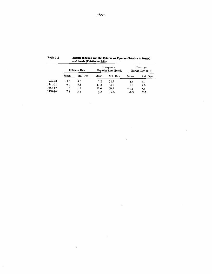
Table 1.2: Annual Inflation and the Returns on Equities(Relative to Bonds) and Bonds (Relative to Bills) 5a
Table 1.3: Business Cycle Reference Dates, 1926—80 6a
Table 1.4: The Geometric Difference Between Returns on Equitiesand Treasury Bonds, Near Troughs, Near Peaks, andin Other Periods 7a
Table 2.1: Explanation of Monthly Realized Returns onTreasury and Corporate Bonds 14a
Table 2.2: Explanation of Monthly Realized Equity Returns, 1953-60 l5a
Table 2.3: Explanation of Monthly Realized Equity Returns, 1961-80 16a
Table 2.4: Explanation of Monthly Realized Equity Returns, 1953-80 17a
Table 3l: Regressions of the Inflation Rate on the Treasury BillRate, 1955—80 23a
Table 4.1: Determination of Semiannual Unanticipated PercentageChanges in the New Iss'ue Coupon Rate 31a
Table Al: Granger Causality Tests A3
Table A2: Granger Causality Tests with Past Inflation Included A5
Table B: McCulloch's Data B4
Table C: The Semiannual Data Base C3
Debt and Equity Yields: 1926—80
Patric H. Hendershott and Roger D. Huang
An important companion to a study of how corporations have issued and
investors have purchased debt and equity securities during the past half-
century is an examination of how these securities have been priced in this
interval. Both resource utilization and inflation have varied widely in the
American economy, causing sharp changes in security prices and thus enormously
diverse ex post returns on corporate equities and bonds. Even if we limit
ourselves to the Post-Accord (1951) years, the variation in returns is huge.
To illustrate, equities earned positive real returns in 1954, 1958 and 1975 of
54, 41, and 30 percent, respectively, but had -24 percent and -38 percent
returns in 1973 and 1974. Variations in real returns on high quality
corporate bonds were smaller, but in the double digit range nonetheless (plus
14 percent in 1970 and 1976 and —13 to —16 percent in 1969, 1974, 1979 and
1980) . The primary purpose of this study is to increase our understanding of
the determinants of these variations.
The study is divided into four broad parts. We begin with an explora-
tory analysis of the data for the 1926-80 period. It makes good analytical
sense to examine the data for any regularities without the imposition of too
much structure before studying the data in the confines of a particular model.
In Part 2, we estimate the relationships between one-month expost returns on
corporate bonds and equities and variations in Treasury bill rates, economic
activity, and other variables. The major other variable is unanticipated
changes in new issue coupon rates on long-term Treasury bonds. Parts 3 and 4
contain econometric investigations of the determinants of one-month Treasury

—2—
bill rates and unanticipated changes in long-term Treasury coupon rates,
respectively. These parts perform two functions; they extend the analysis of
Part 2 by explaining variables that determine expost corporate bond and equity
returns and they provide evidence on the determination of new issue yields on
short— and long-term default-free debt. The first part of the study differs
from the others in that it consists of simple numerical analysis (plots,
calculation of means, etc), rather than formal econometrics, and considers
data from the entire 1926-80 period, rather than the 1953—80 span.
A number of important issues are addressed in the econometric parts of
the paper. These include: the validity of the Modigliani-Cohn valuation-error
hypothesis, the measurement of Merton's "excess return on the market", the
relationship between real new-issue debt rates and real economic activity, and
the usefulness of the Livingston survey data in explaining financial returns.
Three general data sets are analyzed. First, the expost returns on
bills, bonds and equities are those compiled by Ibbotson and Sinquefield
(1980); causality tests of relationship among these returns and inflation are
reported in Appendix A. Second, changes in the coupon rate on long-term, new
issue equivalent Treasury bonds and unanticipated changes in this rate are
based upon the work of Huston McCulloch and are described in Appendix B.
Third, unanticipated inflation and industrial production growth are derived
from the Livingston survey data, and they and the entire semiannual data set
utilized in the analysis of unanticipated changes in new issue coupon rates
are presented in Appendix C.
1. Exploratory Data Analysis
This part of the study contains sections dealing with: (1) inflation
and Treasury bill rates, (2) inflation and relative returns on equities, bonds

—3—
and bills, and (3) the business cycle and returns on equities and bonds.
Before turning to the analysis, a few words about the data are in order.
First, all of the underlying yield data compiled by Ibbotson and Sinquefield
—— equities, corporate bonds, Treasury bonds, and Treasury bills -- are
roughly representative of returns on economy-wide "market" portfolios and are
available monthly for the 1926-80 period. These yields are realized, rather
than expected, returns, except for those on Treasury bills which are both
expected and realized because their one—month maturity equals the period over
which the returns are calculated. Second, the returns—-income plus capital
gains (except for bills) --are before-tax returns. They are not truly
representative of what either highly taxed or tax-exempt investors actually
earned after tax (both investor groups presumably would have opted for
portfolios with relative income and capital gains components different from
the market average, and the former group, of course, paid taxes). Hopefully,
differential returns, at least, are roughly representative of those earned by
most investors.
The inflation rate is the rate of change in the consumer price index for
the 1926-46 period and the rate of change in the consumer price index net of
the shelter component after 1946. The latter circumvents the erroneous
treatment of housing costs (especially mortgage interest) in the construction
of the basic CPI [see Blinder (1980) and Dougherty and Van Order (1982)].
11 Inflation and Treasury Bill Returns
During the 1926—80 period there was a single episode of significant
deflation, 1930-32. In those three years the inflation rate ranged from —6 to
-10 percent. Modest deflation also occurred in 1926—27, 1938, and 1949. In
contrast, there have been three significant bursts of inflation-—the beginning

—4—
of World War II (9 percent in 1941 and 1942) the postwar surge (18 percent in
1946 and 9 percent in 1947) and the Korean War scare (6 percent in 1950 and
1951) --and the prolonged post—1967 inflationary era. The current inflation
has ranged from slightly over 4 percent (adjusting for the impact of price
controls in 1971—72) to double-digit inflation in 1974 and again in 1979-80.
The above overview of the 1926-80 period suggests that division of these
years into four subperiods might be useful. These are 1926-1940 (which
includes the Depression and all years of even modest deflation except 1949)
1941—51 (which includes the inflationary spurts of World War II, its after-
math, and the outbreak of the Korean conflict), 1952-67 (the era of stable
prices), and 1968-80 (the present inflationary period). The first two columns
of Table 1.1 present the mean and standard deviations for the annual inflation
rate for these and overlapping periods. The great differences in the mean
inflation rate and its variability are obvious.
The next four columns list means and standard deviations for both the
nominal and real one-month Treasury bill rate. As can be seen, there is an
enormous difference in the variability of the real bill rate between 1926-51
and 1952—80. In the latter period the standard deviation of the real bill
rate, 1.5 percent, is only three-fifths of that of the nominal bill rate, 2.6
percent; in the earlier period, the former, 6.4 percent, is over five times
the latter, 1.2 percent. Division of the earlier interval into 1926-40 and
1941—51 reveals enormous variability in the real bill rate (and stability in
the nominal rate). The mean real bill was a full 2.8 percent in 1926—40 and
an incredible -5.4 percent in 1941-51. The negative real rate in the l940s
was due to the monetary authorities' policy of pegging nominal interest rates
at low levels during a period of significant inflation. The high real rate in
the 1930s is largely attributable to the combination of the general non-

-4a-
Table 1.1 Annual Inflation and Nominal and Real One-Month Treasury Bill Rates
1926-401941—51
1952—67
1968—80
Inflation Rate Nominal Bill Rate Real Bill Rate
Mean Std. Dcv. Mean Std. Dev. Mean Std. Dcv.
--1.56.01.57.1
4.05.31.23.1
1.3 1.50.6 0.42.7 1.0
6.7 2.2
2.8 4.5—5.4 5.5
1.2 0.8
—0.4 1.8
1926-511952—80
1.74.0
5.93.6
1.0 1.24.5 2.6
—0.6 6.40.5 1.5
Note: The real bill rate is the nominal rate lessthe inflation rate. Annual rates are geometricaverages of the twelve monthly rates during calendaryears.
.300C I I
.2000-
-Nomina /
C —I -I I I\ / /
I..) V
-\/eat
-1000 -
— I I I I I
933 1940 1947 1954 1961 1968 1915 1982
YEAR
Fig. 1.1 Real and Nominal Treasury Bill Rates, 1926-80.

—5—
negativity constraint on the nominal rate and the existence of significant
deflation. However, it is noteworthy that the real bill rate exceeded 4
percent in all years in the 1926-30 period during which the nonnegativity
constraint was not binding (the nominal bill rate ranged from 2.4 to 4.7
percent).
Figure 1.1 illustrates the marked difference between the 1926-51 and
1952—80 periods in the volatility of both the nominal and real bill rates.
In the former period, the nominal rate declines in the early 1930s and is then
flat; in the latter period this rate cycles around a sharply rising trend
(the 1980 average bill rate of almost 12 percent disguises variations in
monthly rates between less than 7 percent and over 16 percent). In contrast,
the real bill rate varied between +12 percent in 1931 and 1932 and -18 percent
in 1946. Its often—cited stability clearly refers to the post—1951 period
1only.
1.2 Inflation and Relative Returns on Equities, Bonds, and Bills
The first two columns in Table 1.2 repeat the same columns in Table 1.1.
The third and fourth columns record the mean and standard deviation of the
difference between the annual returns earned on equities and corporate bonds.
As can be seen, the premium equities have earned over bonds have varied
widely. The premium was much greater in the 1940s, 1950s, and 1960s than in
the 1930s and l970s.2 It would appear from these data that there is no simple
relationship between the premium and either the mean or the standard deviation
of the inflation rate.3
The last two columns in Table 1.2 report the mean standard deviation of
the difference between the annual returns earned on U.S. government bonds and
one-month bills. The difference was extraordinarily large, 3.8 percent, in
CorporateEquities Less Bonds
TreasuryBonds Less Bills
Table 1.2 Annual Inflation and the Returns on EqWtles (Relative to Bonds)and Bonds (Relative to Bills)
Inflation Rate
Mean Std. Dcv. Mean Std. Dev. Mean
1941—51 6.0 5.3 13.2 14.8 1.5 4.01952—67 1.5 1.2 12.6 19.7 — 1.1 5.81968O 7.1 3.1 .o —.s
Std. Dev.

—6—
the 1926-40 period, and small, -2.5 percent, in the 1968—80 period. These
differences are due to apparently unanticipated movements in interest rates.4
To illustrate, if yields fall unexpectedly, then prices of long-term bonds
will rise unexpectedly, and the one-year return on bonds will be large. This
was apparently the case in the 1930s (the one-month bill rate declined from an
average of over 3.0 percent in 1926—30 to less than 0.5 percent in the 1933—40
period). In contrast, if yields rise unexpectedly, then prices of long-term
bonds will fall unexpectedly, and the one-year return on bonds will be low.
This apparently has happened in the post-1952 period (the one-month bill rate
rose from 1.5 percent in 1952—55 to 5 percent in 1967—69 to over 10 percent in
1979-80) .
It is important to note that only unanticipated movements in interest
rates have such impacts on the difference in realized returns on bonds and
bills. For example, if long-term bond rates were expected to rise during the
year, then bonds would be priced at the beginning of the year such that a high
income return would offset the anticipated capital loss. In this case, the
difference in ex post returns on bonds and bills would be independent of
observed changes in new-issue bond yields.
1.3 The Business Cycle and Returns on Equities and Treasury Bonds
In this section, we explore the presence of a business cycle effect on
returns earned on investment in corporate bonds and stocks. The reference
dates of the National Bureau of Economic Research are employed as a general
guide to the stages of the business cycle. In the 1926-80 period, 10½ cycles
have occurred (see Table 1.3) . Excluding the 43 month depression, con-
tractions have ranged from 6 to 16 months and have had an average duration of
11 months. Excluding the 80 and 106 month wartime (World War II and Viet Nam)
expansions, upswings have varied from 21 to 59 months in duration and have

—6a -
Table 1.3 Business Cycle Reference Dates: 1926 to 1980
Business cycle reference dates
Duration in months
Contraction Expansion(previous (trough to
peak to peak)trough)
Trough
November 1927
March 1933
June 1938
October 1945
October 1949
May 1954
April 1958
February 1961
November 1970
March 1975
July 1980
Average, all cycles:
11 cycles, 1926-1980..
5 cycles, 1926—1953..
6 cycles, 1953—1980..
August 1929
May 1937
February 1945
November 1948
July 1953
August 1957
April 1960
December 1969
November 1973
January 1980
21
50
80
37
45
39
24
106
36
59
50b
47b
53b
a. 11 months, excluding the great depressionb. 39 months, excluding the World War II and Vietnam cycles
Source: National Bureau of Economic Research, Inc.
Peak
13
43
13
8
11
10
8
10
11
16
6
10

—7—
averaged 39 months.
Annualized differences in ex post equity and bond returns over different
phases of the business cycle have been compared.6 For contractions, the first
and last 5 months (which overlap for contractions of less than 10 months
duration) were examined. For expansions, the first, second, third, and last
six months were studied (the last two periods overlap during the 21 month
upswing in the late l920s). The cycles were divided into the 1926-52 and
1953—80 subperiods, and means and standard deviations of the differences in
equity and bond returns were calculated for the 5 pre 1953 cycles, the 5½ post
1952 cycles, and all 10½ cycles. A cursory examination of the data revealed
that equities tend to earn a relatively superior return (i.e., greater than
the average 7 percent by which equity returns exceeded bond returns throughout
the entire 1926—80 period) late in contractions and early in expansions and a
relatively inferior return late in expansions and early in contractions.
A systematic comparison of the return data is reported in Table 1.4. We
first divided the months between January 1926 and December 1980 into three
types of periods: those around troughs (in which equity returns appear to be
superior), those around peaks (in which equity returns appear to be relatively
inferior), and the remainder. The inferior periods are defined as the last
six months of every expansion and the first half (dropping fractions) or first
six months, whichever is less, of every contraction. The superior periods are
defined as the last half (dropping fractions) or last six months, whichever is
less, of every contraction and the first six months of every expansion. In
the second step in this comparison, the total 1926-80 period is partitioned
into eleven overlapping intervals that contain single adjoining peaks and
troughs and all the surrounding months that do not overlap with adjacent
superior and inferior periods. That is, the intervals extend from 6 months

-7a-
Table 1.4: The Geometric Difference Between Returns on
Equities and Treasury Bonds, Near Troughs, Near Peaks,and in other Periods (in percent)
Near Near Other Excess ExcessTroughs Peaks Months Near Near
Troughs Peaks
Jan 26 — Feb 29 37 19 17 20 2
June 28 — Nov 36 24 —12 —6 30 —6
Oct 33 — Aug 44 26 —32 8 18 -40
Jan 39 — May 48 31 17 1 30 16
May 46 — Jan 53 35 —10 12 23 —22
May 50 - Feb 57 43 —4 20 23 —24
Dec 54 — Oct 59 46 —10 16 30 —26
Nov 58 — June 69 32 —14 8 24 —22
Sept 61 — May 73 27 —11 6 21 —17
June 71 — July 79 27 —10 3 24 -13
Oct 75 — Dec 80 56a 13b 4c 51 9
Mean 35 —5 8 26 —13
Standard Dev. 10 15 8 11 17
a. covers the period May 80 - Dec 80b. covers the period Aug 79 - April 80c. covers the period Oct 75 - July 79

—8—
after a trough to 6 months before the second following peak. These eleven
overlapping intervals are listed at the left in Table 1.4. Also listed are
the geometric mean returns (annualized) during: the superior periods within
the interval, the inferior periods, and all months excluding such periods.
The mean in the latter months is the normal" return to which the mean returns
around the trough and peak are compared.7
Columns 4 and 5 are the differences between the superior and inferior
returns, respectively, and the normal returns. The extraordinary annual net
returns on equities around troughs average 26 percent (no net return is less
than 18 percent), and the standard deviation is only 11 percent. In contrast,
the extraordinary annual net returns on equities are negative around most
peaks, and these net returns average -13 percent. Here, however, the standard
deviation is a relatively large 17 percent.
These results indicate that investors could devise superior trading
schemes involving transactions between equities and government bonds to the
extent that they were able to forecast the turning points of business cycles,
particularly the recession trough. Given the brevity of the post World War II
recessions, this would not appear to be difficult; when a recession is clearly
upon us, the trough is just around the corner. Unfortunately, such a trading
rule will lead to incredibly negative returns if the early l930s are ever
repeated.
2. Expost Returns and the Interest Rate and Business Cycles
Our next task is to explain expost monthly returns on corporate bonds
and equities. The analytical framework, which follows Mishkin (1978, 1981),
is first developed and then empirical results for bonds and equities are
reported.

-9—
2.1 The Analytical Framework
The expost after-tax return on an asset equals the expected or required
return plus the difference between the expost and expected returns. With the
required return equal to the after—tax return on one—month Treasury bills plus
a risk/liquidity premium, we have
(l-t)R1= (l—T)Rtl+ p + UNEX1, (2.1)
where is the premium required on the jth asset, and UNEXt+1 is the
difference between the expost and anticipated after—tax return on asset j that
occurs because of unexpected changes in variables relevant to the return on
asset j. Next p and UNEXt are replaced by a constant plus a set of
responses to proxies for them (X) and an error term (ni) to obtain
R1 + R1+ =2 + n1, (2.2)
where = (l-T)/(l-T3) . The difficult problem is, of course, specification
of the X.s.
Unanticipated Changes in Treasury Coupons
In section 1.2, it was suggested that changes in new-issue equivalent
20-year Treasury bond yields have been largely unanticipated during the 1952-
80 period. This proposition can be tested with data compiled by Huston
MCulloch. For the 1947-mid1977 period, McCulloch (1977) has meticulously
constructed monthly series for both (1) new issue equivalent (par value)
long-term Treasury bond yields and (2) cumulative unanticipated changes in

these yields.8 A regression of the monthly change in the 20 year new-issue
yield (AR2O) on the unanticipated change (UNA) over the January 1953-June 1977
period results in
AR2O = 1.27 + .999 UNA, R2 = .882 DW = 2.88(.34) (.021) SEE = 5.9 basis points
where the yields are at annual rates. The positive constant reflects the
generally upward 'slope" of yield curves, and the response to unanticipated
changes is clearly one-for-one. The adjusted R2 indicates that 88% of monthly
changes other than the constant are explained by the unanticipated change.
In equation estimates reported below, variables based upon both AR2O and
UN will be employed (the latter in equations excluding data after June 1977).
The specific form of the variables depends on how an unexpected change in the
bond rate should affect the price of (capital gain on) the specific security
being analyzed. The percentage capital gain on a portfolio of n-year bonds
(CGb) is related to changes in the yield on the n year bond, AR, by
AR ((1+RCG=- nb
In the regressions reported below, n is set equal to 20. With CGb defined in
this way, its coefficient is expected to be near unity.
For equities, the relationship between the capital gain component of the
yield and the unanticipated change in the new issue coupon rate is more
complicated. The perpetual dividend growth valuation model says that the
value of equities (V) equals current after-tax dividends [(l_Td)DI divided by
the required after—tax nominal return on equities (Ra) less the expected

—11—
rate of appreciation in dividends (g)
(l_td)DV
a (2.3)Re_ g
Taking derivatives, the percentage capital gain on equities, dV/V, is related
to changes in the 20 year coupon rate by
CGe-
diRa_gi
The issues are: how should R:- g be measured and what is the likely value of
the derivative of Ra g?
Portfolio equilibrium requires that
=(ltd)R2O + p, (2.4)
where bonds and dividends are assumed to be taxed equivalently and p is a
required risk premium. Thus
- g (ltd)R2O + p - g,
and
g)— 1 - dg (2.4)
dR2O—
Td dR2O
Equation (2.4 ) suggests the following. First, if all changes in R20
are due to changes in expected inflation which are, in turn, reflected in g
(dg/dR2O = 1) , then d(R_ g)/dR2O equals - Td and CGe is positive. Second,
for low values of Tds R:- g is roughly constant. This joint hypothesis

—12—
suggests the use of AR2O/0.06 as a regressor, with an expected positive
coefficient of T)° On the other hand, if x percent of changes in R20 are
due to changes in the real rate of interest and thus dg/dR2O = 1 - x, then the
coefficient on the regressor would be - (x -Ta) Ideally, one would separate
changes in interest rates into nominal and real components and enter these in
the regressions separately. Such a separation of monthly changes would seem
to be near impossible and is not attempted here.
An alternative view of equity valuation exists. Equation (2.4) assumes
that investors rationally compare nominal returns on debt and equities. In
contrast, Modigliani and Cohn (1979) have contended that investors compare
real equity returns with nominal debt returns and that this error has been the
cause of the dismal performance of equities during the 1966-80 period of
rising inflation. To test this hypothesis, (2.4) is replaced with
— = (l—Ta)R2O + p . (2.4a)
In this case
- g =(l_Ta)R2O
+ p - g + iT.
Taking derivatives,
d(R_) —1- dg +dir1- (2.4a)
dR2O Td dR2O dR2O Td.
If Modigliani and Cohn are correct, then the appropriate regressor is
AR2O/[ (lTd)R2O+.O4] -- we take the real component of g to be 0.02 -- and the
expected coefficient is - (i-Ta) Whether changes in interest rates are
perceived to be real or nominal is irrelevant (g and iT change equally in any

—13—
event) to investors and thus to equity prices. In the empirical work reported
below, both the rational and Modigliani and Cohn views will be tested. In
these tests, we shall set Td = 0.3 (see footnote 18 for results with other
values of Td).
Of course, R20/.06 and R2O/[ltd)R2O + .04] are closely correlated,
being dominated by their numerators. Thus, if one "works," so will the other.
If neither works, then we will accept the rationality hypothesis with x =
If both work positively, then the Modigliani-Cohn hypotheses will be rejected.
If both work negatively, we will choose between the rationality and
Modigliani-Cohn hypotheses on the basis of the plausibility of the implied
estimates of x and Td•

—138--
Other Variables
In section 1.3, it was established that equities earned extraordinarily
large returns relative to bonds around recession troughs, very likely because
of a turnaround in expectations regarding the growth of the economy. We would
expect this to generate capital appreciation on equities and possibly bonds
(if default premia decline). Based upon the earlier analysis, a turnaround
dummy variable is defined as:11
(1 last half (dropping fractions) or last six months,whichever is less, of every contraction and first
TURN = six months of every expansion
1O elsewhere.
A final proxy is unexpected inflation. This variable is measured as the
difference between actual and expected inflation where the latter is based on
the Livingston survey data.12 More specifically, the variable is the
difference between the actual average monthly inflation rate between the
survey date and the date forecast and the Livingston forecasted six-month
inflation rate converted to a monthly basis. Because the forecasts are
13available only semi-annually, our proxy changes value only every six months.
Because price surprises appear to lead declines in real economic activity --
there is a strong negative correlation between our unanticipated inflation
variable and the growth rate of industrial production in the following year,

—l4
the surprises should be expected to depress equity returns (and possibly bond
returns if default premia rise) l4
2.2 The Results for Bonds
The results for corporate bonds are reported in Table 2.1. Equations
(1) and (2) are for the l953—mid77 period and differ only in that (1) includes
the capital gains variable based upon the unexpected change in the 20 year
Treasury rate as a regressor while the variable in (2) is based upon the
total change.15 Given our earlier evidence that changes in the 20 year rate
are predominantly unanticipated, it is not surprising that the results are
quite similar. The bill rate coefficients are close to their expected value
of unity. On the other hand, the capital gain coefficients are only about
seventy percent of their expected unity value. The unanticipated inflation
and superior dummy variables enter with the expected signs, but only the
coefficient on the former is significantly different from zero at the .05
level.
Equation (3) contains estimates for the entire 1953-80 period. The
coefficient on the bill rate is now quite close to the expected unity value;
and the explanatory power of the equation increases sharply (R2 rises from
0.56 to 0.68) . The coefficient on the capital—gain variable, 0.76, is closer
to unity, but still significantly below, and the other coefficients, while
continuing to have the expected signs, are not significantly different from
zero. These coefficients are not small, however. Bond returns tend to be 2.3
percent less than normal in a year of 2.5 percent unanticipated inflation and
2.3 percent more in the year surrounding business cycle troughs.
2.3 The Results for Equities
Hendershott and Van Home (1973, pp.304-05) observed that the new—issue
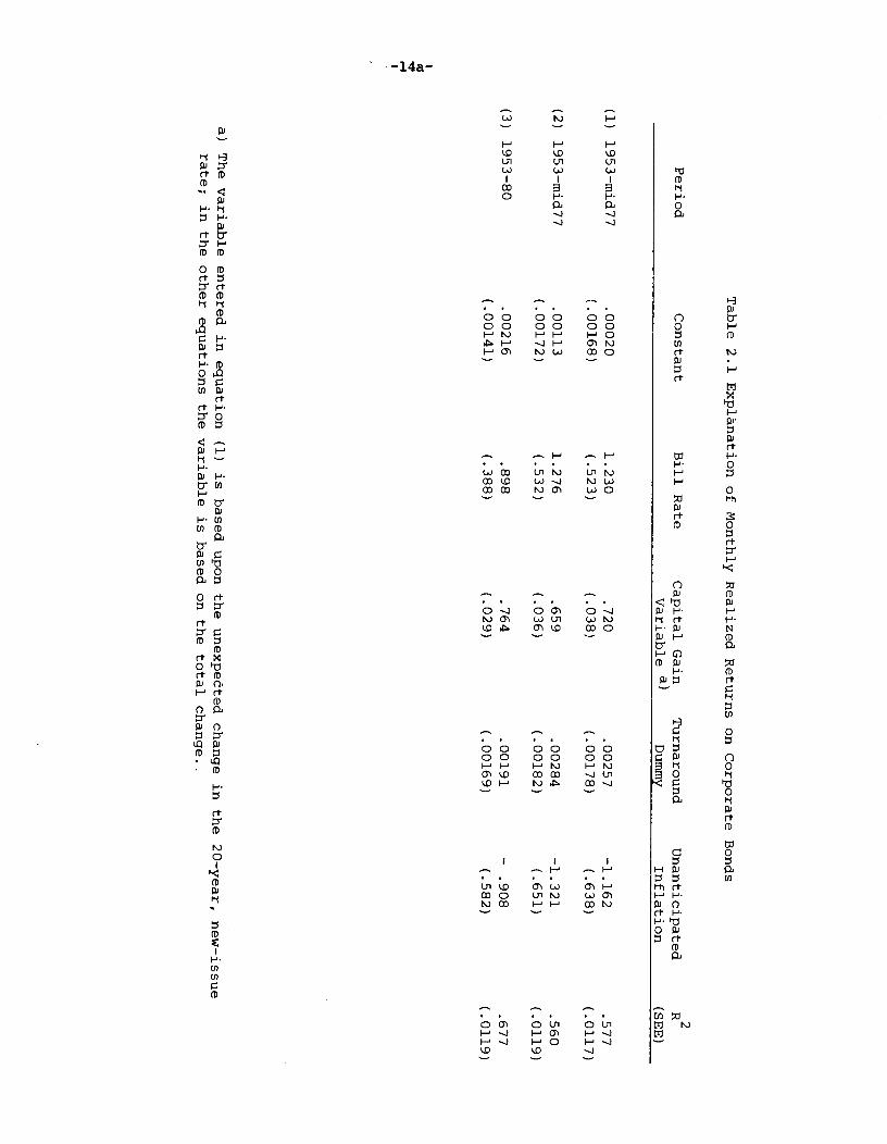
Table 2.1 Explanation of Monthly Realized Returns on Corporate Bonds
Period
Constant
Bill Rate
Capital Gain
Turnaround
Unanticipated
R2
variable a)
Dummy
Inflation
(SEE)
(1) l953—mjd77
.00020
1.230
.720
.00257
—1.162
.577
(.00168)
(.523)
(.038)
(.00178)
(.638)
(.0117)
(2) 1953—mid77
.00113
1.276
.659
.00284
—1.321
.560
(.00172)
(.532)
(.036)
(.00182)
(.651)
(.0119)
(3) 1953—80
.00216
.898
.764
.00191
—
.908 .677
(.00141)
(.388)
(.029)
(.00169)
(.582)
(.0119)
a) The variable entered in equation (1) is based upon the unexpedted change in the 20-year, new-issue
rate; in the other equations the variable is based on the total change. -

—15—
bond yield and Standard and Poor's dividend-price ratio moved in opposite
directions throughout the l950s (they conjectured that a sharp decline in the
relative risk premium required on equities occurred) but were positively
correlated in the l960s and early 1970s. Consequently, the 1953-80 period is
divided into the 1953-60 and 1961-80 subperiods and results are reported for
these.
Equation (1) in Table 2.2 illustrates the familiar, but hardly expli-
cable, result that ex post equity returns were strongly negatively correlated
16with expected inflation in the 1950s. The point estimate is an astounding
—16, indicating that a one percentage point increase in the bill rate
(expected inflation?) induced a 16 percentage point decline in equity returns.
Equation (2) indicates the expected negative relationship with our
unanticipated inflation variable (the average monthly inflation rate between
the date the Livingston survey was taken and the date forecast less the
Livingston forecasted six-month inflation rate) and positive relationship with
the turnaround cycle dummy variable, but neither relationship is statistically
significant. Equations (3) and (4) include current and lagged one-month
values of the variables based upon changes in the long-term Treasury coupon
rate. The variables in equations (3) and (5) are the Modigliani-Cohn
nominal-rate versions defined as LiR2O/(.7 R20 + 0.04); the variables in
equations (4) and (6) are the real—rate versions defined as AR2O/0.06. A
one—month lag was tested because equities and new-issue bonds are not as close
substitutes as are corporate and Treasury bonds. Recall that the coefficients
in (3) are expected to be negative and sum to -0.7 if investors make the
Modigliani-Cohn valuation error (and the tax rate on dividends is 0.3),
and the coefficients in (4) can be interpreted as —(x —Td)1 where x is the
portion of changes in R20 due to changes in real coupon rates and Td is the

Table 2.2: Explanation of Monthly Realized Equity Returns, 1953-60
Changes in
-2
One-Month
Unanticipated
Turnaround
Coupon Rate a)
R
Equ.
Constant
Bill Rate
Inflation
Dummy
Current
Lagged
(SEE)
(1)
.0410
—16.005
.108
(.0086)
(4.494)
(.0336)
(2)
.0315
—10.752
—3.457
.0139 .115
(.0112) (5.528)
(3.410)
(.0096)
(.0335)
(3)
.0263
—8.173
—4.069
.0154
.397
—.282
.173
(.0112)
(5.452)
(3.410)
(.0095)
(.173)
(.176)
(.0323)
•
(4) .0262
—8.125
—4.084
.0155 .362
—.262
.167 (.0112)
(5.467)
(3.418)
(.0095)
(.163)
(.165)
(.0324)
(5)
.0095
1.0
—5.606
.0244
.421
—. 285
.163 (.0051)
(3.318)
(.0079)
(.174)
(.177)
(.0327)
(6)
.0095
1.0
—5.628
.0245
.384
—.268
.163
(.0052)
(3.323)
(.0079)
(.164
(.167)
(.0327)
a)
This variable equals R20/ (.7 R20 + .04) in the odd numbered equations and AR2O/.06 in the even
numbered equations.

—16—
tax rate on dividends. A positive relation between equity returns and the
concurrent change in the bond yield is indicated, although the impact is
largely reversed the following month.17 This is inconsistent with the
Modigliani-Cohn hypothesis and supports the rationality hypothesis. The
implied dividend tax rate, assuming that changes in interest rates are
perceived as nominal (x = 0), is 0.1 (when the lagged term is taken into
account) to 0.36.
While the bill rate coefficient is still a startling -8 in equations (3)
and (4), it is not significantly different from the expected unity value. In
equations (5) and (6) this coefficient has been constrained to unity. As
anticipated, the decline in explanatory power is minor. The impact of changes
in Treasury coupon rates is unchanged from equations (3) and (4) , but the
coefficients on unanticipated inflation and the turnaround dummy rise in
absolute value and statistical significance (the t-ratios are 1½ and 3,
respectively)
Equations for the 1961-80 period are listed in Table 2.3. While the
Treasury bill rate enters negatively in equation (1), the coefficient is only
a tenth as large as that in equation (1) of Table 2.2. Moreover, when
unanticipated inflation and the turnaround dummy variable are included, the
bill rate coefficient is close (given its standard error) to unity. The
coefficients on unanticipated inflation and the turnaround dummy have the
expected signs and are significantly different from zero. Equations (3) and
(4) contain the change in coupon-rate variables. The coefficients in equation
(3) sum to -0.6, very close to the expected value of —0.7 in the Modigliani-
Cohn framework (further lagged values of the variable have essentially zero
coefficients), and the variables add substantially to the explanatory power of
equation (2)18
The coefficients in equation (4) sum to —0.33, implying that

Table 2.3:
Explanation of Monthly Realized Equity Returns, 1961-SO
Change in
-2
One-Month
Unanticipated
Turnaround
Coupon Ratea)
R
Equ.
Constant
Bill Rate
Inflation
Dummy
Current
Lagged
(SEE)
(1)
.0147
—1.575
.001
(.0066)
(1.352)
(.0417)
(2)
.0025
2.162
—6.437
.0253
.085
(.0071)
(1.906)
(2.491)
(.0071)
(.0399)
(3)
.0020
2.770
—6.062
.0215
—.326
—..Z12
.149 (.0069)
(1.87?)
(2.425)
(.C)070)
(. 099)
(.101)
(.0385)
(4)
.0005
3.173
—6.479
.C)222
—.178
—.156
.141
(.0070)
(1.907)
(2.441)
(.0070)
(.060)
(.062)
(.0387)
'U
(5) .0075
1.0
—4.445
.0227
—.5333
—.254
.156
(.0036)
(1.714)
(.C)069)
(.098)
(.099)
(.0385)
(6)
.0073
1.0
—4.507
.C)237
—.181
—.139
.147
(.0036)
(1.723)
(.C)069)
(.060)
(.060)
(.0387)
a)
This variable equals AR2O/(L7 R20 +.04) in the odd numbe•réequations and R20/O6 inthe even
numbered equations.

—17—
most of changes in long-term coupon rates (one-third plus the dividend tax
rate) have been perceived by rational investors (not Modigliani-Cohn
investors) as changes in real rates. The rationality of this perception,
during a period of rising inflation, is questionable.
When the bill rate coefficient is constrained to unity [see equations
(5) and (6)], the other coefficients are little affected except for that on
unanticipated inflation which falls by a quarter in absolute value. Because
its standard error falls proportionately, the statistical significance of the
coefficient is unaltered.
Comparison of equations (5) and (6) in Table 2.2 with their counterparts
in Table 2.3 indicates a close similarity of all coefficients except those on
the current change in the Treasury coupon rate. Given this similarity,
equations for the entire 1953-80 period have been estimated and are reported
as equations (1) and (2) in Table 2.4. The estimates are, of course, close to
those of the subperiods. The coefficients in equation (2) can be interpreted
in the following way. First, the constant term, which is 0.102 on an annual
basis, represents Merton's excess expected return on the market. Second, the
bill rate contributed an average 4½ percent return over the period, rising
steadily from under 2 percent in the early 1950s to over 10 percent in 1979—
80. Third, the continuing climb in the Treasury coupon rate lowered stock
returns by nearly 2 percent per annum on average during the 1953-80 period.
More importantly, the change in this rate has had large impacts in particular
years. To illustrate, the percentage increase in the coupon rate from 9
percent to 12½ percent between March 1979 and March 1980 generated a 15
percent expost decline in stock returns in that year, other things being
equal. Fourth, the coefficient on the turnaround dummy variable suggests that
equities have earned a 34 percent greater return in the year roughly

Table 2.4:
Explanation of Monthly Realized Equity Returns, 1953-80
Change in
-2
One-Month
Unanticipated Turnaround
Coupon Ratea) Presidential Term Dummies
R
Equ.
Constant
Bill Rate
Inflation
Dummy
Current
Lagged
Year 2
Year 3
Year 4
(SEE)
(1)
.0084
1.0
—5.082
.0238
—.189
—.264
.139
(.0030)
(1.501)
(.0054)
(.086)
(.087)
(.0374)
(2)
.0081
1.0
—4.948
.0244
—.131
—.155
.140
(.0030)
(1.502)
(.0053)
(.055)
(.055)
(.0374)
(3)
.0022
1.0
—3.695
.0264
-.200
—.260
—.0040
.0115
.0088
.153
(.0048)
(1.564)
(.0055)
(.085)
(.086)
(.0059)
(.0050)
(.0058)
(.0371J
(4)
.0016
1.0
—3.521
.0271
—.138
—.152
-.0038
.0117
.0094
.156
(.0048)
(1.566)
(.0055)
(.055)
(.055)
(.0059)
(.0058)
(.0058)
(.0370)
a)
This variable equals tR20/ (7 R20 +
.04) in the odd numbered equations and t R20/.06 in the even
numbered equations.
—18—
surrounding business cycle troughs than during other periods. Fifth, stocks
have earned sharply negative returns, ceteris paribus, during periods of
unanticipated inflation. More specifically, the roughly 4½ percentage point
unanticipated inflation in 1973—74 and 1979 translates into a 22 percent lower
annual return on equities than would otherwise be the case. Our
interpretation of this negative relation between equity returns and
unanticipated inflation is that the latter generates expectations of tighter
monetary policy and thus both higher interest rates and sluggish economic
l8aactivity.
As is well known, equity returns follow a strong political cycle. For
example, during the 1953-80 period equity returns averaged 3½ percent in the
two years following presidential elections, but 20 percent in the two years
leading up to the elections. Because the political cycle is so readily
predictable, such differences in returns must certainly be attributable to
other factors which, it just happens, have been correlated with the business
cycle in the past but might well not be in the future. Likely candidates for
these other factors are the interest rate and business cycles as reflected in
our change—in—coupon, turnaround, and unanticipated-inflation variables. To
determine whether our equations have captured the observed political cycle
impact, we have computed the annual errors from equation (2) in Table 2.4 and
averaged them over the first and second pairs of years of presidential terms.
Much to our surprise, the difference in these averages was a full 13 percent.
That is, our equation accounts for only 3 of the 16½ percent average
difference in average returns between the two years leading up to presidential
elections and the two following years.
The last two equations in Table 2.4 include political cycle dummy
variables that equal one in months which fall in the second/third/fourth year
of presidential terms and zero in all other months. As can be seen, their

—19—
inclusion raises the explanatory power of the equations. Moreover, the
hypothesis that the coefficients on the three political-cycle dunimy variables
are jointly zero can be rejected at the .05 level. Inclusion of these
variables does not affect the interest rate coefficients, but it does alter
the others by one-half (the turnaround dummy and the constant terms) to a full
(unanticipated inflation) standard error.'9
3. Treasury Bill Returns and the Inflation Rate
3.1 Theory
Definitionally, the real rate of interest is the nominal interest rate
less the inflation rate. If we let r+1 and Rt+i be the real and nominal
interest rates earned over the holding period t to t+l, respectively, and
be the inflation rate over the same time span, then
r+1 Rt+1 - 1t+] (3.1)
Taking expectations of both sides of (3.1) contingent on information available
at t, so that expectations are formed rationally, (3.1) becomes
r R — 11 , (3.2)t t+l t+l t t+l
where is the real rate expected at time t to exist in period t+l,tt+1
is the inflation rate expected at time t to exist in period t+1, and (3.2)
utilizes the fact that the expected nominal interest rate is the expost rate
because Rt÷, is known at time t. In a world where lenders are required to pay
an income tax rate t on their nominal interest receipts and borrowers can

—20—
deduct T percent of their nominal interest payments,
(lT)Rt+i - tt+l, (3.2a)
where r÷i is the expected after-tax real short-term rate.
The expected inflation rate is the difference between actual and
unanticipated inflation: tt+l +l - UNINFt+l. With this substitution in
(3.2a), one can obtain
1t+l -r+1 + (l-T)Rt+l +UNINFt+i.
If the expected after—tax real short-term rate and t are constants and the
unanticipated rate of inflation is white noise, then it is appropriate to
regress 't+l Rt÷1 and a constant. The equation is estimated with inflation
as the dependent variable and the interest rate as the independent because the
latter is predetermined while the former develops during the period.
Unfortunately, a large body of evidence rejects the assumption of a constant
real rate [see Garbade and Wachtel (1978), Mishkin (1981) and the references
cited in the latter], and the Livingston inflation survey data indicate
systematic inflation forecast errors. The purposes of our estimation are to
provide evidence on the determinants of the real short-term rate and to test
for the presence of systematic errors in inflation forecasts.
3.2 Problems with the Inflation and Interest Rate Data
Fama (1975) regressed inflation on the bill rate on data from the
January 1953 - July 1971 period. He ruled out the data from World War II and

its aftermath owing to both the low quality of the CPI prior to 1953 and to
the Federal Reserve's pegging of nominal interest rates. Given constant
nominal rates and highly variable inflation, the real bill rate varied widely.
Our earlier examination of the 1926-39 period suggests that there, too,
nominal bill rates were relatively stable (near zero in the l930s) and real
bill rates relatively volatile. Thus we also restrict ourselves to the post
1952 data.
Fama did not extend his analysis beyond July 1971 because the CPI was
contaminated beginning in August 1971 by the Nixon price controls. Because
"true" inflation is relevant to the nominal bill rate, regressions of recorded
inflation on the nominal bill rate may give misleading results when true and
recorded inflation rates differ. Subsequently, many investigators, including
Fama, have proceeded to analyze data from the control period with no
adjustments. In order to utilize post July 1971 data in our tests, we include
a proxy for the difference between recorded and true inflation in our
regressions. In constructing this proxy, we utilize the results of Blinder
and Newton (1981). More specifically, we use the change in their Model I
measure of the impact of the controls on the nonfood, nonenergy consumer price
index as our proxy for the difference between recorded and true inflation.20
Their results suggest that the controls reduced the price level by 3
percentage points by early 1974, a reduction which was completely offset when
the controls were lifted in 1974.
A more general problem with the consumer price index is the treatment of
housing costs (especially mortgage interest) in the construction of the index
[see Blinder (1980) and Dougherty and Van Order (1982)1. To circumvent this
problem, the inflation rate employed in this paper is the consumer price index
net of the shelter component. Such an adjustment is particularly important in

—22—
analyzing data after 1978.
A final possible data problem follows from a phenomenon documented by
Cook (1981). He notes that in 1973 and 1974 short-term bill rates became far
"out of line" relative to short—term rates on large CDs, commercial paper, and
bankers acceptances. During this period market interest rates rose sharply
relative to ceiling-constrained yields on deposits. According to Cook, the
bill market was segmented from markets for private short-term securities.
Because only bills were available in smaller denominations, many households
were able to shift deposit funds only into bills. Corporations did not have
sufficient bill holdings to arbitrage between the bill and private security
markets (they drew their holdings down to zero in 1974), and commercial banks
and municipalities had nonyield reasons for maintaining bill holdings. Thus
bill rates fell relative to other yields. As a result, expected inflation was
not fully reflected in bill rates. In fact, the enormous disparity between
private and Treasury short-term yields in 1974 was the driving force behind
the creation of the money market fund, an entity that, in the absence of other
government regulations, should prevent such disparities from recurring21
During the 156 month 1965-77 period, the spread between one-month prime
CDs and one-month Treasury bills was generally within the 30 to 80 basis point
range.22 Two major exceptions occurred. During the 20 months from April 1969
to November 1970, the spread exceeded 90 basis points in 17 months and was at
maximum of 189 basis points in July 1969. During the 24 months from April
1973 to March 1975, the spread exceeded 90 basis points in 23 months, the
maximum being 431 basis points in July 1974. In the 4 years prior to April
1969, the spread was above 80 basis points in only 4 of 48 months and never
exceeded 110 basis points. In the 28 months between November 1970 and April
1973, the spread exceeded 81 basis points only once (85 basis points in July

—23-
1972). Finally, in the 39 months between April 1975 and June 1978, the spread
never exceeded 90 basis points.
In the empirical estimates, then, we specify the inflation rate as the
CPI net of shelter, the price control variable CONT is included in regressions
using data from the August 1971 - December 1974 period, and both the observed
one month Treasury bill and an adjusted rate that moves with the CD rate when
the bill rate is out of line are utilized as regressors.
3.3 The Estimates
Table 3.1 contains the regression coefficients (and their standard
errors, under them in parentheses), the coefficient of determination (and the
equation standard error, under it in parentheses), and Durbin—Watson ratio for
equations explaining the rate of change in the CPI net of shelter over the
January 1953 - December 1980 span.23 In the first two equations, it is
assumed that (a) the real after—tax bill rate is either a constant or a linear
function of the nominal after-tax bill rate and (b) unanticipated inflation is
white noise. As can be seen, the bill rate coefficient is significantly above
unity. This result is similar to that obtained by Fama and Gibbons (1981,
Table 1) in their study of data from the 1953-77 period. Because tax rates
cannot be negative, this estimate implies that the after-tax real bill rate is
negatively related to expected inflation (and thus to the after-tax nominal
rate).24 To illustrate, if r+1 = - tt+l' then the use of (3..2a) and the
inflation identity (inflation is the sum of its expected and unexpected
components) yields
1t+l = - + + UNINFt+1. (3.4)
The coefficient on the nominal rate will be greater than unity if >-r.25 A

Table 3.1 Regressions of the Inflation Rate on the Treasury Bill Rate, 1953-80
Constant
—.00120
(.00029)
2
— .00109 (.00029)
3
— .00099 (.00028)
4
— .00095 (.00027)
5
—.00133
(.00018)
6
— .00082 (.00027)
7
— .00090 (.00026)
a)Except equation (7) where an
.539
(.194)
.231
(.191)
.215
(.190)
.222
(.190)
1.0
495
(.00258)
.744
.545
(.124)
(.00245)
—.00909
.879
.555
(.00295)
(.123)
(.00243)
—.00862
.753
.158
(.00295)
(.104)
(.00244)
—.00889
.744
.504
(.00302)
(.121)
(.00249)
—.00933
.782
.559
(.00293)
(.126)
(.00241)
See the text for the adjustment.
Equation
1
Bill Ratea
Price Controls
Variable
Capacity
UtI1.834
Unanticipated
Inflation
2
R
(SEE)
.484
(.00260)
1.220
(.069)
1 . 190
(.069)
.920
(.080)
.857
(.075)
1.0
.863
(.076)
.846
(.073)
adjusted
IJurbin
Watson
1.47
1.50
1.61
1.64
1.64
1.58
1.63
.029
(.188)
bill rate series is used.

—24—
negative relation between real after—tax debt rates and expected inflation is
hardly surprising when the use of historic-cost depreciation and FIFO
inventory accounting erodes after-tax real earnings of firms during periods of
rising inflation. Because firms are unable to pay constant real after-tax
returns to debtors and shareholders in the aggregate, the returns to each
would be expected to decline (Hendershott 1981, pp. 913—14)
Examination of the residuals from equation (2) reveals that they tend to
be negative in the l950s and 1960s and positive in the 1970s. That is, the
equation overpredicts inflation in the early years and underpredicts it later.
Two possible explanations come to mind. First, the real bill rate may have
fallen between the l960s and l970s by even more than is captured by the high
coefficient on the bill rate and the increase in this rate. If real interest
rates are positively correlated with real economic activity, then the
relatively sluggish activity in the l970s would suggest a decline in the real
26rate.
Second, possibly more of the higher inflation in the l970s was
unanticipated than was the case in the 1950s and 1960s. Comparison of actual
six-month inflation rates with the forecasts computed from the Livingston
Survey data suggests that this was the case (see Appendix C). Four periods of
prolonged unanticipated inflation (four consecutive large six month
forecasting errors) occurred: the four surveys from June 1956 to December
1957, January 1969 to June 1970, January 1973 to June 1974 and June 1978 to
December 1979. Not only did two of these come during the shorter period of
large positive residuals, but the average degree of unanticipated inflation
was 4½ percent (at an annual rate) in these two vis-a-vis 2½ percent for the
earlier episodes.
Equation (3) is the result of including a proxy for unanticipated

—26—
inflation, Of course, if the real bill rate were a constant and the proxy for
unanticipated inflation were perfect, then we would be estimating an identity,
the usefulness of which could be easily questioned. What is being tested in
equation (3) is whether an unanticipated inflation variable based on the
Livingston survey data (see page 13 above) improves on the assumption of white
noise. The proxy enters with the anticipated positive sign and yields a
marked improvement in explanatory power. Moreover, the coefficient on the
bill rate is lowered below unity, although not significantly so. Equation (3)
is consistent with the joint hypotheses that the real Treasury bill rate was
constant during the 1953-80 period (at a 1.2 percent annual rate) and that the
Livingston survey data are slightly high estimates of unanticipated inflation.
In equation (4) we test the hypothesis that real bill rates are related
to real economic activity. As a proxy for real activity, we follow Carlson
(1979) and Hendershott and Hu (1981) in using the Federal Reserve's capacity
utilization rate for manufacturing. Because this rate is available only
quarterly, we assign this value to the middle month of the quarter and
interpolate linearly between mid-quarter months. This series, lagged one—
month and divided by 100, less its mean value over the 1953—80 period of 0.834
is the regressor. This variable enters with the expected negative sign and
has a t—ratio of 3,27 The coefficient on unanticipated inflation rises to
within a standard error of unity and that on the bill rate falls to nearly two
standard errors below unity.28
Fama and Gibbons (1981), among others, have provided evidence that
expected real bill returns behave like random walks. If this is true of real
bill returns even after allowing for their positive relationship with real
economic activity, then the nominal bill rate is correlated with the error
term and thus its estimated coefficient is biased downward. Equation (5)

—26—
provides estimates of the other coefficients when that on the bill rate is
arbitrarily constrained to unity. The standard error of the equation rises
ever so slightly and the coefficient on unanticipated inflation falls to 0.75.
The adjusted R2 indicates that one-sixth of the variation in inflation after
allowing for variations in the bill rate is explained by variations in
unanticipated inflation and capacity utilization.
To this point, the coefficient on the price controls variable has not
been discussed. In equation (2), the coefficient is statistically different
from both its maximum plausible value of unity and its minimum plausible value
of zero. In subsequent equations, the coefficient is about 0.2 or only one
standard error from zero. Although the controls variable is nonzero in only
the August 1971 - December 1974 period, its coefficient could affect the
coefficients on the other variables because all variables move sharply in this
period. To test this sensitivity, equation (4) was rerun with the controls
coefficient arbitrarily constrained to unity. Equation (6) indicates that
only the coefficient on unanticipated inflation is affected, declining to
0.75.
Our last experiment tests an adjusted bill rate variable which takes
into account the fact that bill rates were out of line relative to private
open—market rates during much of the April 1969 - March 1975 period. In April
1975, the first month after bill rates returned to the normal relationship
with private rates, the one-month bill rate was 0.004347. The bill rate was
almost precisely the same in November 1968, shortly before it got out of line.
In this month, the one-month CD rate exceeded the bill rate by 0.00047. The
adjusted bill rate series is defined as the CD rate less 0.00047 during the
November 1968 - March 1975 period and the bill rate otherwise. This adjusted
series replaces the observed bill rate in equation (7). Relative to equation

—27—
(4), the coefficients on the price controls and unanticipated inflation
variables decline by a standard error, and the explanatory power of the
equation rises slightly.
3.4 Summary
Three findings should be emphasized. First, the existence of price
controls and out-of—line bill rates in the early and middle l970s do not have
an important impact on the estimates. Inclusion of the price controls
variable or adjustment of the bill rate improve the explanation of inflation
slightly, but the values of the important regression coefficients are largely
unaffected.
Second, the real bill rate is shown to be systematically related to the
level of real activity as measured by the capacity utilization rate. With the
coefficient of the latter equal to -0.009, the real bill rate is 2½ percentage
points higher (at an annual rate) when the utilization rate is 90 percent than
when it is 70 percent.
Third, the estimated responses of actual inflation to both expected
inflation (as reflected in the bill rate) and unanticipated inflation (based
on the Livingston survey data) are close to unity. The bill-rate coefficient
point estimate is 0.85, while that of the unanticipated inflation varies
between 0.74 and 0.88. Although the lowest of these coefficients is two
standard errors below unity, we do not emphasize this because there is reason
to believe that the coefficients may be biased downward. Unfortunately, the
tax rate of the representative investor cannot necessarily be inferred from
the bill rate coefficient. For example, an estimate of unity implies a zero
tax rate if the real bill rate is independent of the expected inflation rate,
but a positive tax rate if the real bill rate is negatively related to

expected inflation, a relationship that would be reflected in the estimated
bill rate coefficient. The significance and empirical importance of the
unanticipated inflation measure suggests that the Livington survey data, which
indicate a significant underestimate of six month inflation throughout much of
the 1969—80 period, may well have accurately reflected the expectations of
market participants. This underestimate of expected inflation explains why
nominal bill rates failed to move one-for-one with actual inflation during the
1952—80 period.
4. The Determinants of Unanticipated Changes in Treasury Coupon Rates
In Part 2, expost returns on corporate bonds and equities were shown to
be strongly influenced by unanticipated changes in long-term new issue
Treasury coupons (or by total changes which were shown to be largely
unanticipated). The last stage of our study is an investigation of the
determinants of these unanticipated changes.29 We begin with the analytical
framework and then report some equation estimates.
4.1 The Framework
Unanticipated changes in long-term Treasury rates are caused by changes
in long-run expected inflation, which are unanticipated by definition, and
unanticipated changes in the long-term real rates. Of course, neither of
these is observable. Thus the problem is to specify proxies for expected
inflation and the expected real rate and, for the latter, to distinguish
between anticipated and unanticipated changes.
The results of Parts 2 and 3 give us some guidance here. From the
Livingston survey, we have estimates of expected short-run inflation. While
the validity of this survey data is questioned by some, the empirical

—29—
significance of the measure of unanticipated inflation based on these data in
both the equity-return and inflation regressions suggests that the data have
empirical content. It seems reasonable that long-run inflationary
expectations would be revised upward in response to unanticipated short—run
inflation.
The inflation equations also implied that real Treasury bill rates are
related positively to the capacity utilization rate. Short—run changes in
this rate, in turn, must be closely correlated with the growth rate of
industrial production. As a consequence, it is reasonable to hypothesize that
unanticipated changes in long-term rates are positively correlated with
deviations between actual and expected growth rates in industrial production.
Fortunately, the Livingston survey also contains forecasts of industrial
production six months ahead.
Because the Livingston survey data are available only semiannually (June
and December) , the analysis of unanticipated changes in Treasury coupon rates
is conducted in a six-month time frame. That is, changes from December of one
year to June of the next, from that June to the next December, etc., are the
dependent variable in the analysis (the specific data are discussed and listed
in Appendix C). We denote the change from t-l to t as UNAt. This change is
hypothesized to depend on unanticipated industrial-production growth, UNIPtS
and unanticipated inflation, UNINFtI between t-l and t. These variables are
defined more precisely as
UNIPt = [IP — Eti(IPt)]/IPt1UNINFt It - Et1(It),
where IP is the level of industrial production, I is the inflation rate (the

-30—
subscript t denotes inflation from t-l to t) and E is the expectations
operator.
Policy surprises must also be accounted for because they may provide
information beyond that incorporated in the above defined variables. This
would likely be true to the extent that policy surprises affect prices and
real income with a lag; if the full impact occurred instantaneously, it would
be reflected in the unanticipated inflation and industrial production growth
variables. The most obvious surprise in the 1955—80 period was the imposition
and removal of price controls in the early l970s. To proxy this surprise, we
specify a controls dummy variable that assumes the value —l in the second half
of 1971 when the controls were imposed, 1 in the first half of 1974 when the
controls were removed, and 0 in all other periods. To the extent that the
imposition and removal of controls, respectively, lowered and raised expected
long-run inflation, this variable, PCDUM, should have a positive impact on the
change in coupon rate.
The fiscal surprise variable employed is that computed by von
Furstenberg (1981). This variable is defined as the difference between the
actual and "normal" surpluses of Federal, state and local governments, divided
by net national product. The normal surplus takes into account not only the
stage of the business cycle but also regular (forecastable) discretionary
policy actions taken over the course of the business cycle (regular tax cuts
during recessions, for example). This variable is denoted by FSUR. The
variable exceeds 1½ percent, in absolute value, in only three periods: 1960,
mid1966 - midl968 (the Vietnam buildup), and the second quarter of 1975 (the
extraordinary tax rebate). A positive fiscal surprise (unusually large
surplus) would be expected to lower interest rates. The decline would be
relatively minor if the surprise does not lead to a revision in the "fiscal

31—
policy" rule. Von Furstenberg argues persuasively that this was the case in
the 1955-78 period.
The monetary surprise variable tested is the difference between the rate
of growth in the adjusted monetary base computed by the Federal Reserve Bank
of St. Louis and the growth rate in recent periods (say the previous two
years). The impact of this variable on interest rates is unclear.
Unanticipated monetary growth would tend to depress real rates (Milton
Friedman's "liquidity effect") but to an upward revision in the inflation
premia.3° Because the estimated coefficient on variants of this variable
never had a t—ratio greater than one or an estimated impact greater a few
basis points, equation estimates with this variable are not reported below.
We would expect that the coupon rate would be linearly related to the
unanticipated inflation and price control variables as constructed. Because
the unanticipated industrial production and fiscal surprise variables are real
ratios, we would expect them to impact on the percentage change in the new
issue coupon rate. To reflect these considerations, the unanticipated change
in the coupon rate, unanticipated inflation, and the price controls variable
have all seen deflated by the lagged value of the twenty-year Treasury coupon
rate. Thus the estimated equations are of the form:
UN/R2O1 = O + + 2UNINF/R2O1-
3FSUR+
4PCDUM/R2O1 (4.1)
where 0 and > 0 for i>0.
4.2 The Estimates
The first equation in Table 4.1 is estimated over the 1955-78 period,
the span for which von Furstenberg calculated his fiscal surprise variable.

Table 4.1:
Determination of Semiannual Percentage Unanticipated
Changein the New Issue Coupon Ratea)
Unanticipated
Price
-2
md. Prod.
Unanticipated
Fiscal
Controls
R
Period
Constant
Growth
Inflation
Surprise
Dummy
(SEE)
1955—78
—.0107
.0082
.0535
-.0129
.660
.340
(.0109)
(.0020)
(.0281)
(.0066)
(.268)
(.0519)
H
1955—80
—.0074
.0093
.0578
—.0128
.646
.331
(.0115)
(.0021)
(.0292)
(.0071)
(.287)
(.0557)
a)
The dependent variable, unanticipated inflation, and the price-controls dumniy are deflated
by the beginning-of-period, 20-year, new-issue coupon rate.

—32—
All variables enter significantly with the expected signs, the constant term
is within a standard error of zero, and the equation explains a third of the
variance in the dependent variable. The sources of the cumulated 6 percentage
point rise in the new issue coupon rate over the 1955-78 period are
unanticipated six-month inflation and industrial production growth; both
averaged 1.3 percentage points per period in this span. Multiplication of 1.3
by 48 semiannual periods and the relevant regression coefficient yields 3.3
percentage points for the cumulative effect of unanticipated inflation. To
obtain the impact of unanticipated industrial production growth, we multiply
1.3 by 48, the regression coefficient (.0082), and the mean value of the
twenty-year Treasury coupon in this period, 5.4. The result is 2.8 percentage
points. A single 4½ percentage point inflation error, which occurred during
1973—74 and again in 1979, is accompanied by a quarter of a percentage point
rise in the coupon rate. The production growth forecasting errors exceeded
+0.06 in six semiannual periods between 1955 and 1978, but were never larger
than the 0.0082 coefficient implies that a 0.08 underforecast of
industrial production growth is associated with a two—thirds percentage point
increase in the new issue coupon when it is at the 10 percent level. A
relatively large negative fiscal surprise, such as the 2½ percentage point
surprise during the mid66 - mid68 Vietnam buildup, is accompanied by a 15
basis point per period rise in the coupon rate. Finally, the imposition of
price controls appears to have lowered long-run inflation expectations by
nearly two-thirds of a percentage point.
The second equation in Table 4.1 contains estimates for the full 1955-80
period. In this equation the fiscal surprise variable was arbitrarily set
equal to zero (the variable was 0.404 in the fourth quarter of 1978 and
averaged -0.187 during the 1955-78 period). Because there were not any
—33-.
obvious surprises in the last two years of the Carter administration, this is
probably a reasonable approximation. The estimated coefficients are close to
those of the first equation with the exception of the response to
unanticipated growth which rises by half a standard error. The actual and
predicted percentage changes from this equation are plotted in Figure 4.1. As
can be seen, the equation seems to underpredict a number of large changes
(except those associated with price controls), but does capture major swings
in the new issue coupon (except possibly the most recent one).
With the fiscal surprise variable still maintained at zero, our equation
significantly overpredicts the level of the Treasury coupon rate in 1981 and
1982, even allowing for the sharp decline in late 1982. This is to be
expected for two reasons. First, a substantial fiscal surprise has
undoubtedly occurred. While taxes are normally cut during recessions and the
1982 full employment deficit is not large by historical standards, the
combination of the July 1983 tax cut, the indexation of taxes in future years,
and the difficulties of controlling many expenditures leads to large "out
year" full employment deficits. This "permanent" surprise could have had a
quite large impact on interest rates. Second, the sharp 1981 cut in the
taxation of returns from business capital would be expected to raise real
interest rates by a percentage point or two (Hendershott and Shilling 1982).
5. Sunmary
This study began with an examination of data for the 1926-80 period on
returns earned on one—month Treasury bills, long-term Treasury and corporate
bonds, and corporate equities. Relationships among the returns and between
them and inflation and the business cycle were identified. We then turned to
econometric investigations of the relationships between expost monthly returns

-——
——
—+
——
——
——
—+
——
--——
——
+—
—
630 650
670
690
710
730
750
uS
DATE
Firri. 41 P
UN
DR
2O 551—
802
US
ED
IS -
____________ -
PLO
T OF PUNDRHAT*DATE
SYMBOL USED IS +
UNOR2O
0.05
0.00
-0 .15
—0.20
530
570
590
610

-34-
on corporate securities and bill rates and other variables, principally the
unanticipated change in the coupon on new issue Treasury bonds. We concluded
with an investigation of the determinants of the bill rate and the
unanticipated change in long—term Treasury coupon rates.
The most general theme of the econometric work is the usefulness of the
Livingston survey data in explaining financial returns. Unanticipated
inflation, defined as the difference between short—run observed inflation and
the Livingston forecast, enters the equity-returns, inflation-rate, and
change—in—new—issue—coupon equations significantly. (When unanticipated
inflation is not included as a regressor in the inflation equation, the
estimates imply that real (bill) interest rates are negatively related to
expected inflation; when unanticipated inflation is included, this negative
relationship does not appear to exist.) In addition, changes in new-issue
coupon rates are positively related to unanticipated growth in industrial
production, defined as the difference between observed growth and the
Livingston forecast.
The latter result is part of a secondary theme, a positive relationship
between real interest rates or returns and real economic activity. Expost
equity returns ("the market") are strongly related to expectations of future
economic activity. In every business cycle since at least 1926, the market
has risen sharply around cycle troughs (the last half or six months, whichever
is shorter, of recessions and first six months of expansions); other things
being equal, equity returns are 34 percentage points higher during this key
year of turnaround in expectations than these returns are at other times. In
addition, unanticipated inflation, which appears to lead to expectations of
]kwer real economic activity, deprssesequityivalues (by as much as 22
percent in 1973-74 and 1979), other things being equal. The investigation of

—35—
new—issue debt yields lends supporting results. The real Treasury bill rate
is positively related to the capacity utilization rate with the real rate
being 2½ percentage points higher when utilization is at 90 percent than when
it is at 70 percent. Because more rapid growth in industrial production leads
to higher capacity utilization, the relationship between changes in new issue
rates on long-term Treasuries and this growth is implicitly a relationship
between the level of Treasury bond rates and capacity utilization.
Unanticipated changes in new Treasury coupon rates (and 88 percent of
monthly changes during the 1953-77 period were unanticipated) are the dominant
determinant of expost monthly corporate bond returns and also strongly
influence equity returns. Regarding the latter, a 2½ percentage point
increase in new issue Treasury coupon rates is estimated to lower the market
by 10 percent. More generally, for the 1961-80 period the data are consistent
with the Modigliani-Cohn valuation-error model and a dividend tax rate of
about 0.4. Finally, a third of semiannual percentage unanticipated changes
in new issue coupon rates over the 1955—80 period can be explained by
unanticipated six-month inflation and industrial production growth, fiscal
policy "surprises," and the imposition and removal of price controls in the
early 1970s.
The analysis of the present study can usefully be extended in two ways.
First, a switch to a semiannual data base for all parts of the empirical work
is called for in order to more appropriately utilize the Livingston survey
data. This switch might also allow some differentiation in the effects of
real and purely nominal unanticipated bond rate changes on equity returns.
Our analysis was not able to distinguish between Modigliani-Cohn irrationality
(there is no need to differentiate between changes in real rates and in
inflationary premia because investors only care about their sum) and

-36-
rationality (with much of nominal rate changes being real changes) because it
is near impossible to identify inflationary premia in long-term bond rates on
a monthly basis. Second, the stability of the estimated relationships over
time should be tested. It would, of course, be useful to know if the
relationships have been altered by the change in Federal Reserve operating
procedures and the resulting increased volatility in financial markets since
October 1979. Preliminary examination of the movement in long-term Treasury
coupons indicates that a change has likely occurred.

37 Hendershott& Huang
Footnotes
1The variability in the real bill rate in the 1952—80 period would likely have
been even lower in the absence of deposit rate ceilings. More specifically,
the large negative values in 1973 and 1974 are due to bill rates becoming "out
of line" relative to private short-term yields due to disintermediation (see
p. 22 below).
2The premium that equities earned over Treasury bills is similar to the extent
that returns on bonds and bills are roughly equal. As is indicated in the
last column of Table 1.2, government bonds outperformed government bills by
nearly four percentage points per annum in the 1926-40 period, with the result
that the equity premium over bills was significantly greater than that over
bonds. The reverse was true, although to a lesser degree, in the 1968—80
period.
3Nonetheless, many have attributed the poor performance of equities in the
1969-78 decade to increased inflation and/or uncertainty regarding inflation.
Feldstein (1980) has argued that biases in the tax law reduce share values in
inflationary periods, while Modigliani and Cohn (1979) have attributed the
reduction to an inflation-induced error of investors. Malkiel (1979) has
contended that increased uncertainty regarding future price and government
regulation changes has lowered share values by increasing the relative risk
premium demanded on equity investments. In contrast, one of us has argued
that these phenomena explain the relatively modest rise in promised new-issue
debt yields (decline in real after—tax yields), but not the sharp decline in
share values (Hendershott 1981).
4Shiller (1979) has suggested that changes in long-term bond coupon rates have

—38—
been largely unanticipated.
5Huston McCulloch has constructed the unanticipated changes in long-term
Treasury coupon rates in the 1947-77 period. These data are discussed in
Appendix B and are employed in the econometric work in Parts 2 and 4 below.
6Th• comparison is reported in Hendershott (1982).
7The annualized geometric return over N periods on an asset earning R in
period i is [II(l+R.)-l]'2.i=l 1
8Both of these series are described in Appendix B.
10We value (l_Td)R2O — g at zero and p at 0.06.
11Because there was also weak evidence that equities earned negative returns
relative to bonds around business cycle peaks, a negative turnaround dummy
variable was defined analogously to the positive one and tested. The
coefficient on this variable was never near a standard error from zero in any
bond or equity equation.
'2The Livingston survey data have been questioned by Pearce (1979) on the
grounds that they are not rationa1" and are less consistent with observed

—39—
bill rates than are rational inflation expectations. On the other hand,
Mishkin (1981) is unsure that the the Livingston data are irrational, and
Carlson (1981) makes a strong argument that "irrationality" might not be
surprising.
13The precise series used equals (1. + UNINFA/lOOY1"12 - 1, where UNINFA is
from the semiannual data base listed in Appendix C.
'4When Carlson and Kling (1982) specify expected inflation from an ARIMA model
and test for lead or lags between unexpected inflation and real activity via
bivariate autoregressions, they, too, find price surprises leading real
activity negatively.
15The Durbin—Watson statistics for the equations in Table 2.1 vary between
2.25 and 2.45.
16See Bodie (1976), Jaffee and Madelker (1976), Nelson (1976), and Fama and
Schwert (1977).
17The Durbin-Watson statistics for the equity equations over the different
time periods vary between 1.95 and 2.15.
18The equation might be interpreted as suggesting a higher tax rate on
dividends; with t,R2O/(.55 R20 +.04) as the regressor, the coefficients would
sum to —.45. With AR2O/(R20 +.04) as the regressor, the coefficients sum to
—0.75.

—40—
l8aThere is an alternative interpretation. Because unanticipated inflation is
greatest precisely when oil shocks occurred, this variable may be capturing
nothing more than the negative impact on share values of the unexpected
increase in energy prices. We will attempt to distinguish between these two
interpretations in future work.
19The "true" constant term which abstracts from political cycle effects is
obtained as the sum of the coefficients on the political dummies and four
times the estimated constant, all divided by 4. For equations (3) and (4)
the true constants are 0.0063 and 0.0059.
20The data are from their Table 2, p. 17.
21The spread between private rates and bills could also be affected by changes
in risk and in the level of interest rates. The latter could matter because
the income from private securities is taxed at the state and local level while
that from bills is not.
22The CD rates are first of month data recorded by Salomon Brothers.
Cochraine—Orcutt semi—difference transformation -- with a semi-difference
parameter of 0.15 to 0.25 —- lowers the equation standard error for all of the
equations in Table 3.1 but hardly changes the coefficient estimates.

—41—
24Thus the result is also consistent with Mishkin's findings (1981) for
quarterly data from the 1953-79 period. When the lagged inflation rate is
added to equation (3.2), the procedure followed by Mishkin, the coefficient is
0.3 and the coefficient on the bill rate declines by a similar amount.
25For the derivation of a non-zero from a structural model, see Melvin
(1982)
26The Federal Reserve's capacity utilization rate for manufacturing averaged
84.3 percent during 1953-69 versus 81.4 percent for 1970-80. With a desired
ratio of 90 percent, this is a 50 percent increase in the shortfall.
27The result differs from Mishkin (1981) who does not find a significant
implied relationship between real bill rates and either real GNP growth, the
GNP gap, or the unemployment rate.
28When the lagged inflation rate is added to equation (4), a coefficient of
0.18 is estimated with a standard error of 0.05, and all other coefficients
decline by roughly 18 percent. That is, the result is consistent with a very
short lagged response (18 percent after the first month) to all variables.
290n the relationship among new issue coupon rates on alternative long-term
debt instruments, see Cook and Hendershott (1978), Hendershott, Shilling and
Villani (1982) and Van Home (1978)
30Melvin (1983) provides evidence that the liquidity and inflation effects
exactly offset six months after an increase in monetary growth.

-42- Hendershott& Huang
References
Blinder, Alan S. 1980. The consumer price index and the measurement of recent
inflation. Brooking Papers on Economic Activity 2: 1980:539-565.
Blinder, Alan S. and Newton, W.J. 1981. The 1971-74 controls program and the
price level. Journal of Monetary Economics 8: 1-24.
Bodie, Zvi. 1976. Common stocks as a hedge against inflation. Journal of
Finance 31: 459—470.
Carison, John A. 1977. A study of price forecasts. Annuals of Economic and
Social Measurement 6: 27—56.
_______________ 1979. Expected inflation and interest rates. Economic
Inquiry 17: 597—608.
_______________ 1981. Perceptions (or misperceptions) of inflation. In
Gale, W.A., ed., Inflation: Causes, consequents, and control.
Oelgeschlager, Gunn and Main.
Carlson, John A., and Kling, John L. 1982. Do price surprises lead or lag
real activity? Krannert Working Paper No. 809. Purdue University.
Cook, Timothy Q. 1981. Determinants of the spread between treasury bill and
private sector money market rates. Journal of Economics and Business
33: 177—187.
Cook, Timothy Q., and Hendershott, Patric H. 1978. The impact of taxes, risk,
and relative security supplies on interest rate differentials. Journal
of Finance 33: 1173—1186.
Dougherty, Ann and Van Order, Robert. 1982. Inflation and housing costs.
American Economic Review 72: 154-164.

—43—
Fama, Eugene F. 1975. Short term interest rates as predictors of inflation.
American Economic Review 65: 269—282.
1977. Interest rates and inflation: The messages in the
entrails. American Economic Review 67: 487-496.
Fama, Eugene F. and Schwert, G.W. 1977. Asset returns and inflation. Journal
of Financial Economics 5: 115—146.
Fama, Eugene F. and Gibbons, Michael R. 1981. Inflation, real returns, and
capital investment. Journal of Monetary Economics 7: 296—323.
Feldstein, Martin S. 1980. Inflation and the stock market. American Economic
Review 70: 839—862.
Garbade, Kenneth and Wachtel, Paul. 1978. Time variation in the relationship
between inflation and interest rates. Journal of Monetary Economics 4:
755—765.
Hendershott, Patric H. 1981. The decline in aggregate share values: Taxation,
valuation errors, risk and profitability. American Economic Review 71:
909—922.
_____________________ 1982. Inflation, resource utilization, and debt and
equity returns. In Friedman, B.M., ed. The changing roles of debt and
equity in financing U.S. capital formation. National Bureau of Economic
Research, Chicago. University of Chicago Press.
Hendershott, Patric H. and I-lu, Sheng Cheng. 1981. Inflation and extraordinary
returns on owner occupied housing: Some implications for capital
allocation and productivity growth. Journal of Macroeconomics 3. 177-
203.
Hendershott, Patric H. and Shilling, James D. 1982. The impacts on capital
allocation of some aspects of the Economic Recovery Tax Act of 1981.
Public Finance Quarterly 10: 242—274.

—44—
Hendershott, Patric H. and Shilling, James D., and Villani, Kevin E. 1982.
The determination of home mortgage rates: Empirical results for the
1975-81 period. Paper presented at a joint session of the American
Finance Association and the American Real Estate and Urban Economics
Association meetings, December 1982, in New York City.
Ibbotson, Roger G. and Sinquefield, Rex A. 1980. Stocks, bonds, bills, and
inflation: Historic returns (1926-1978). Charlottesville. Financial
Analysts Research Foundation, University of Virginia.
Jaffee, Jeffrey and Mandelker, Gershon 1976. The "Fisher Effect" for risky
assets: An empirical investigation. Journal of Finance 31: 447-458.
Malkiel, Burtin G. 1979. The capital formation problem in the United States.
Journal of Finance 34: 291-306.
McCulloch, J. Huston 1975. The tax-adjusted yield curve. Journal of Finance
30: 811—830.
___________________ 1977. The cumulative unanticipated change in interest
rates: Evidence on the misintermediation hypothesis. Cambridge,
Massachusetts, National Bureau of Economic Research Working Paper No.
222.
Melvin, Michael. 1982. Expected inflation, taxation, and interest rates: The
delusion of fiscal illusion. American Economic Review 72: 841-845.
_______________ 1983. The vanishing liquidity effect of money on interest:
Analysis and implications for policy. Economic Inquiry: forthcoming.
Merton, Robert C. 1980. On estimating the expected return on the market.
Journal of Financial Economics 8: 323-361.

—45—
Mishkin, Frederic S. 1978. Efficient markets theory: Implications for monetary
policy. Brookings Papers on Economic Activity 3: 1978: 707-752.
____________________ 1981. The real interest rate: An empirical
investigation. In The costs and consequences of inflation. Carnegie—
Rochester Conference Series on Public Policy.
___________________ 1981. Monetary policy and long-term interest rates: An
efficient markets approach. Journal of Monetary Economics : 29-55
___________________ 1981. Are market forecasts rational? American Economic
Review 71: 295—306.
Modigliani, Franco and Cohn, Richard A. 1979. Inflation, rational valuation
and the market. Financial Analysts Journal March-April 1979: 24-44.
Nelson, Charles R. 1976. Inflation and rates of return on common stocks.
__________________ 31: 471—482.
Comparing survey and rational measures of expected
of Money, Credit, and Banking 11: 447-456.
The volatility of long-term interest rates and
of the term structure. Journal of Political Economy
Journal of Finance
Pearce, Douglas K. 1979.
inflation. Journal
Shiller, Robert J. 1979.
expectations models
87: 1190—1219.
Van Home, James C. 1978.
Cliffs, New Jersey.
Von Furstenberg, George M.
Financial market rates and flows. Englewood
Prentice-Hall, Inc.
1981. Saving. In Aaron, H.J. and Pechman, J.A.,
ed., How taxes affect economic behavior. Washington, D.C. The
Brookings Institution.

Hendershott& Huang
Appendix A: Granger Causality Tests
The purpose of this appendix is to investigate the information content
of past returns on bonds (equities) in determining equity (bond) yields after
accounting for past yields on equities (bonds). The role of the inflation
rate is examined in this context both by introducing it as a determining
factor for asset yields as well as by comparing the behavior of nominal and
real asset yields.
The statistical tool we use here corresponds to a statistical test for
exogeneity commonly known as the Granger causality test. It should be empha-
sized that the word causality is used here only in the restrictive sense of
predictability. More specifically, we say that a time series X Granger
causes another time series if we are able to better predict in the sense
of a lower mean squared prediction error by using the past values of both X
and than by employing only the past values of Y.
Specifying the predictor to be a linear one, the test involves
regressing on lagged Ye's and X's, i.e.,
k1 k2Y = c.Y + Z .X .. (A)t it—i it—ii=i i=l
If the parameters ., i=l,. . ,k2, are significantly different from zero, then
X Granger causes or is informative in the prediction of In order to test
the predictive content of in determining X, the roles of and X in (A)
are reversed.
If, contrary to (A), the relevant information set contains variables other
-I2-
than and then the above regression test may show spurious causality
between X and if the other variable leads both X and Y. Given the
results of the previous section, it is therefore highly probable that a test
of the predictive relationship between corporate bonds and stocks will reveal
Granger causality; the causality being the result of shocks that are common to
both stocks and bonds.
In our tests, we specify k1=k2=6. It is felt that 6 months is long
enough to reflect any price adjustments. A constant term and time trend are
added to (A) in the estimation to capture the presence of deterministic
components.
In Table Al we report the results of the tests of the bivariate rela-
tionships between equity and debt returns. The overlapping sample periods
reported are the entire sample 1926-1980, the pre-Treasury Accord period
1926-1952, the pre-Treasury Accord period after the Great Depression 1933-
1952, and the post-Accord span of 1953-1980. Reported are the F-statistics
for tests of the null hypothesis that all the 's in (A) are zero. The tests
are performed for both the nominal and real rates of return.
With one exception, returns on government bonds or bills contain no
informative content in the prediction of equity returns. The reverse is also
supported. The sole exception is the informativeness of government bonds in
predicting stock returns during the post-Accord period. As for common stocks
and corporate bonds, the latter Granger—caused the former when the whole
sample is utilized. However, when sub-periods of the entire sample are
examined, the causality is in the opposite direction with corporate bonds
leading stocks for the 1926—1952 period. When the Depression years are
excluded from the 1926—1952 period, no causality in either direction was
observed. Finally, both equity and corporate bonds appear to be valuable in

Table Al:
Granger Causality Tests
6
Y
c+5_c.. y
t
1
1:—
i i=
1
6 +
i=l
X_ +
(St
Not
e:
The following notations are used:
CS for common stocks, CB
for corporate bonds, TB for Treasury bills.
X and Y variables
refer to the same variables in equation
(A)
in the text.
* de
note
s significance at the 5 percent level.
Variables
Y
X
Sample
F
— S
tatis
tic:
m,n
Period
Nominal
Real
m,n
CS
CB
1926—
3.130*
4.172*
6,640
CB
CS
1980
1.273
1.653
6,640
CS
CB
1926—
2.596
2.444
6,304
CB
CS
1952
6.199*
6.276*
6,304
CS
CB
1932—
1.413
1.852
6,220
CB
CS
1952
0.913
1.093
6,220
CS
CB
1953—
2.950*
3.512*
6,316
CB
CS
1980
3.452*
3.260*
6,316
CS
GB
1926—
2.203
3.104*
6,640
GB
CS
1980
1.267
0.686
6,640
CS
GB
1926—
1.131
1.038
6,304
GB
CS
1952
0.443
0.630
6,304
CS
GB
1933—
0.215
0.691
6,220
GB
CS
1952
0.491
0.328
6,220
CS
GB
1953—
3337*
3.808*
6,316
GB
CS
1980
2.478
2.113
6,316
CS
TB
1926-
1.871
2.414
6,640
TB
CS
1980
2.427
1.530
6,640
CS
TB
1926—
0.945
1.352
6,304
TB
CS
1952
0.771
1.085
6,304
CS
TB
1933—
1.138
2.493
6,220
TB
CS
1952
0.954
1.808
6,220
CS
TB
1953—
1.398
2.187
6,316
TB
CS
1980
1.716
1.239
6,316

-A4-
predicting one another in the Post—Accord period. These observations are
virtually unchanged whether real or nominal returns are used.
In Table A2, we reexamine the results of Table Al by focusing on
nominal returns but with past inflation rates added as a possible
additional source of information. The results indicate that past inflation
rates by themselves do not contain information content. Moreover, the same
conclusions drawn from Table Al with respect to common stocks and corporate
bonds can be drawn from Table A2 when the null hypothesis tested is that both
past X and I have no informative content in predicting Y once one has
accounted for past values of Y. Also similar to Table Al, in general no
distinct causal patterns emerges when government bonds or bills are used in
place of corporate bonds.
To summarize, the results indicate the usefulness, in the post-Accord
period, of past corporate bond (stock) returns in predicting current corporate
stock (bond) returns even after allowing for the presence of past corporate
stock (bond) returns. This result is observed when either nominal or real
returns are used as well as when past inflation rates are added as additional
sources of information. As for government bonds or bills when examined with
stocks, no consistent lead or lag relationships were uncovered. It may very
well be that the Granger causalities observed for corporate bonds and stocks
are due to variables other than the inflation rate that affect both the
variables being examined.

Table
A2:
Granger Causality Tests with Past Inflation Included
6
6
6
=
C +
a. +
ix
t_i
. —j +
i=
1 i=l
i=l
Variables
Y
X
Sample
F
Statistic m,n
F
Statistic
m,n
Period
m,n
m,n
CS
CE
1926—
1.751
6,634
2.451*
12,634
CB
CS
1980
0.542
6,634
0.905
12,634
CS
CB
1926—
1.141
6,298
1.872
12,298
CB
CS
1952
0.884
6,298
3534*
12,298
CS
CB
1933—
1.845
6,214
1.646
12,214
CB
CS
1952
1.704
6,214
1.317
12,214
CS
CB
1953—
1.573
6,310
2.277*
12,310
CB
CS
1980
1.548
6,310
2.518*
12,310
CS
GB
1926—
1.685
6,634
1.784
12,634
GB
CS
1980
0.465
6,634
1,440
12,634
CS
GB
1926—
0.999
6,298
0.972
12,298
GB
CS
1952
0.431
6,298
0.597
12,298
CS
GB
1933—
2.206
6,214
1.690
12,214
GB
CS
1952
0.887
6,214
0.919
12,214
CS
GB
1953—
2.277
6,310
1,854
12,310
GB
CS
1980
3.465*
6,310
2.630*
12,310
CS
TB
1926—
1,576
6,634
1.895
12,634
TB
CS
1980
0.303
6,634
0.781
12,634
CS
TB
1926—
0.935
6,298
1.033
12,298
TB
CS
1952
0.445
6,298
0.442
12,298
CS
TB
1933—
1.872
6,214
1.046
12,214
TB
CS
1952
1.573
6,214
1.036
12,214
CS
TB
1953—
1,367
6,310
2.364*
12,214
TB
CS
1980
1.634
6,310
2.071
12.310
Note: The following notations are used:
CS for common stocks, CB for corporate
bonds, TB for Treasury bills, and I is the inflation rate.
X and Y vari-
ables refer to the same variables in equation
(A)
in the text.
* de
note
s significance at the 5 percent level.

Hendershott& Huang
Appendix B: The McCulloch Data
Our analysis of ex post bond and equity returns employed changes
in the long term, new issue equivalent Treasury bond rate arid the unanti-
cipated change in this rate as regressors. Both of these variables
have been computed by Huston McCulloch (1975, 1977) who developed a
technique of curve—fitting the term structure of interest rates from
security prices so as to determine implicit forward interest rates as
precisely as possible. At each point in time for which Treasury security
prices are available, a discount function is estimated, using a cubic
spline tax-adjusted technique, to give the value at these points of
a promise to repay a dollar at alternative future dates. Before-tax
equivalent instantaneous forward rates, single payment yields, and
par bond yields were calculated from the parameters of the splire discount
curve for maturities sufficiently close to allow linear interpolation
to all desired intermediate points. The tax adjustment was especially
important in the late l960s and early 1970s when all long term Treasury
bonds were selling at substantial discounts owing to effective restrictions
against new issues between 1965 arid 1973 and the sharp rise in interest
rates after the mid l960s (see Cook and Hendershott, 1978).
Except for tax-exempt and selected flower bonds (those whose
prices were determined by the flower bond characteristic), virtually
all U.S. Treasury bills, notes and bonds have been analyzed monthly since
January 1947 (McCulloch updates the file a number of times per year).
The data presented in columns (4) and (3) of Table are the level and
change in the new issue equivalent semi-annual coupon yields on 20 year
Treasury bonds or on the longest possible maturity computable with

B2
MCulloch's technique. During the 1952-81 period the longest maturity
was below 19 years only in the 1970-72 period.
Column (1 of Table contains McCulloch's measure of unanticipated
monthly changes in the longest term Treasury rates, ignoring liquidity
premia (MCulloch, 1977, Appendix 3). This is the difference between the
one-month forward par bond yield and the observed corresponding spot
par bond yield one month later.
In our analysis of semiannual changes in long-term interest rates,
we have updated McCulloch's data on a semiannual basis. Here, we compute
the difference between six-month forward par bond yields (b*) and the
observed corresponding spot par bond yield six months hence (R201).
The unanticipated change (tJNL) is thus
UNL =R201
- b*,
where b* is the semi-annual coupon rate that will make the value of a
bond in six months, evaluateclat the current term structure, just equal
to par, discounted to the present using the current term structure. To make the
calculations, we use as inputs McCulloch's semi-annual coupons (y) on
six month (0.5 years) and 20 1/2 year bonds and continuous single-point
par discount yields (d) on the same maturity bonds. First, the semi-
annual coupons are converted to continuous equivalents
c = 2 log(l + y/2) for maturities 0.5 and 20.5.
Second, the continuous forward par bond yield is computed as
- e05d0.5- e2OSd20.
[1 - e2Sd2O.5]/c20- [1 - e05d0.5]/c0'5

Finally, this continuous yield is converted to a semiannual coupon
equivalent:
b* = 2(e2 1).
Unanticipated changes for the first half of 1977 (December 1976--
average of beginning and end of month values- -to June 1977) through the
first half of 1982 are listed in Appendix C.
The percentage changes in yields employed in the stock return
equations are the changes (R2O or UN) divided by the end of period
value of R20.

r'
i ooraw
m
OO
OO
-.OO
OO
OO
OO
oOO
OO
OO
OoO
OO
OO
OO
cOO
QO
OO
S
.S • S 55.55...••• SeS...•S• SS S S5 S S• SS • • S • •• •.SS 555•••SSe • S
S S
S •S
.SS
SS
• S
*5 I
I ,I
III I
I I
II I
2 G
-.0O'Jm
mm
t'.-4mor- o-?
ooo-. —
jemr-,
.OO
00000000-40-4r r'4O
OO
O40-.IO
OO
4OO
CO
00OO
-4000.O00o0o0000O
0000O0O
OO
O0000O
O
' S
SS
SS
5SI5S
SS
S5S
5SS
S55S
555s5e5555S SSSSSSSSSISSSSSSSSSSSSSSSSSSS•SSSSSIS
000000000000000000000000000000000QQ 0000000OO0O000000O000O0000O00O00OOO
II I
II III
III I
I 1111
II II
11111 III
I I
III III O
gQO
0ooooooo00, —oooooooooooooooooo-oooooooo
I)
m
m
—m
o m
Iru'O
m0-oO
Ø4P
. •*5I•S
SeS
SIS
SS
SS
SS
S•S
SS
SS
SS
SS
SS
SS
.S...•@
..SS
,..S..S
5•I S5S•SSSSSSS5SS5SSSS
rm cmm mmm m
mm
m.
r)
*u' -
ImeIO 's
mtnq,mtom mo ar-nm
in cimm p-
.r -4mJa4.4.4
0000
400C'JO
0-iO('J000..40000 O
O-a0O
QO
O.4Q
Q0O
OQ
0 -.0OO
Oea9i.s0..s 0000—
ooroo of.4o..sie0Oo
•S 55555555*5555 S.5•,,OSSSS SSS$SS•SSS •SSSSISSSSSS5 55,05 •.S•55••• 55S5 55555
ooieoooeooooooaooaa I
II II
I I
III II
I I
I I
00mooN
40p.. 0000-4000 0-400-.0.-'O
OO
-.oOO
0 00000000 30 00000000 040'44N
*O.4 000000-..4000..400*..000
.5555 5SISSS5 IS...,., SS•SSSSSS• 55555555555•••5 5S
S5 •
SS5SSSS5SS5S5 S....
00000000000000000000003000000000000000000000000000000 000o0000000O
OoQ
oO
I II
11111 II
I III
II II
II I
I I
II I
II II
o--.m
o.
Qo-
00OOo0OO
-4000000000 O
OO
O0O
OO
OI..4..4O
QO
OQ
OO
OO
.._4OO
OO
O 0O
00-0OO
OO
OO
OO
—.4
m mm
mmcflmmm
Ifl4C
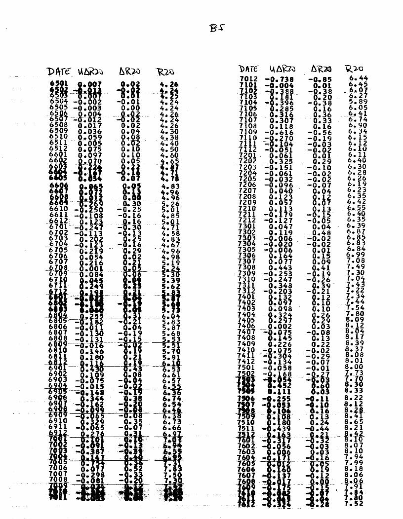
c4QN
Q-4'
p omm
Om
O
Oo-sm
ooor...mm
f4 •S**SSIaaØ
assa.,,.,S,a,,S,,,
r
• • • • • • , .
a • • a • . , •
•
, , .
a • • • a a • a a a a • a a a 0 0 0 0 0 0 0 0 0 I •• I
I a • • •
a a 0
0 I •
• I
0 • •
• 0 1
1
____
isis sits
ii is
'ii I
111111 V
T
III, oo
oom. m
or r- eom
-cm
-in c'np A
i A
Ofl
, Of1
OO
'fl4OO
QO
.-.Q .th-$ O
'4000'40-P 4N
mN
,-oo mO
O
orn-4o.4o OP
-s.4'*flOO
.Oa4ouO
.4OO
! —
&
I •.I0•0o I US
a.. •00..0 •.a •I.aoaal a 'a •asII0aolsIIIa 1.1.10...,. .,.,a.i,.. .•.•
5 ?
Q00O
OO
OO
OO
OO
OO
OO
OQ
OO
OO
OO
OO
OO
OO
QO
OQ
OO
OO
OQ
OO
bøO
** oO0oO
poooO*o
____ OO
CO
....-.-IOQ
OQ
OO
OF
q &
L-U
is . •w.aaj
f4f*4..40 rtjr
Ln(*OP
u. - -
r' 00000000000.-4-40*-40 ••••
a tiiaIS iiI• Ie.a ..*0aiaIllS
SI
0?0?00r0c0000r Øin
'J..4WlQ
fI —
O
NO
4-)O4t'J'
*• ,.aI.I.a
OOOOOOOOPOOOOOC
)OO
C
I I I
S
I $
I I I I
fl4 ,O
ØC
.ial OOC
I I r 4ØWi$C •.. )QO
C
I I I —
am
a ei •ai )OaC
I $
)øW
C
4.u44 •,* *O
C
I 3 4C
P
5VU
W
I... )O
OC
I I
JO
*_e O4rjQ
p*o r.ut
*or- 4P-P
' 1901 I'P
.-. *-a
- —
-- - - -
inO0in'4Q
$*9 ___ O
OC
OO
0OO
000000a4O
- •i• a
.asaoss a:..s • I •
SIII,IIS000I
•••0
——
— —
—
——
——
—
- C
l.a •. I eti •
II •Il II 1.01 I I S S
0O0OOCJD00C O
OC
)OO
C IO
OC
00C
—
I $ I
I I
• jII I II
I I I I I I
I I I
I I 1$
'-4Nm
in o—oo
jo 'OP0 im
sin or—
a..a ,0000 0O
00-44,-.00O6O
inA
ininL(uAiA
tA O
'.OO
r-r-P
-5.- ouo'O
O
i0000Ioo 00 oooO

rc kM1-O
ffIS i1ff 111 fl7705 —0.037 —0.02 7.757706 —0.064 —0.03 7.727707 • —0.16 7.5677Q . 0.09 7.65710' • —0.06 7.597710 • 0.08 7.677711 • 0.22 7.897712 • —0.02 7,87801 • 0.12 7.97802 • 0.15 8.141803 . 0.40 8.247804 • 0.u8 8.327805 • 0.07 8.397806 • 0.17 8.567807 • 0.11 8.677808 . —0.07 8.607809 • —0.18 8.427810 • 0.22 8.647811 • 0.267812 . . —0.12 8.787901 • 0.21 8.997902 • —0.117903 • 0.22 9.107904 •. —0.04 9.067905 • 0.19 9.257906 • —0.15 9.107907 • —0.26 8.84ZQ • 2.42 1.r9yv •79&0 • u.j 9.7911 • 1.13 10.4l,1 • —g. Q.• Iv.8002 • 0.93 U. .8003 '34 '2. .88004 . ö.03 12.518005 • —1.51 11.00:8008 • 0.80 11.018009 • 0.51 11.528010 • 0.44 . 11.968011 . 0.50 12.468012 • 0.11 12.57
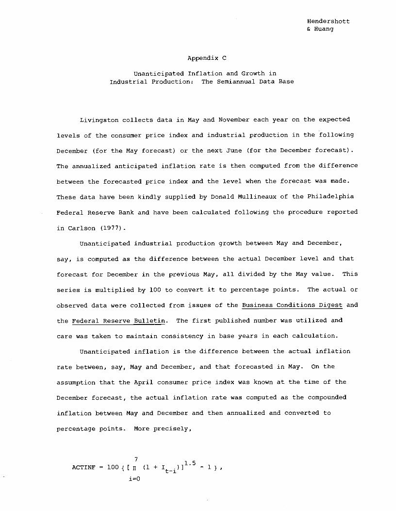
Hendershott& Huang
Appendix C
Unanticipated Inflation and Growth inIndustrial Production: The Semiannual Data Base
Livingston collects data in May and November each year on the expected
levels of the consumer price index and industrial production in the following
December (for the May forecast) or the next June (for the December forecast).
The annualized anticipated inflation rate is then computed from the difference
between the forecasted price index and the level when the forecast was made.
These data have been kindly supplied by Donald Mullineaux of the Philadelphia
Federal Reserve Bank and have been calculated following the procedure reported
in Carlson (1977).
Unanticipated industrial production growth between May and December,
say, is computed as the difference between the actual December level and that
forecast for December in the previous May, all divided by the May value. This
series is multiplied by 100 to convert it to percentage points. The actual or
observed data were collected from issues of the Business Conditions Digest and
the Federal Reserve Bulletin. The first published number was utilized and
care was taken to maintain consistency in base years in each calculation.
Unanticipated inflation is the difference between the actual inflation
rate between, say, May and December, and that forecasted in May. On the
assumption that the April consumer price index was known at the time of the
December forecast, the actual inflation rate was computed as the compounded
inflation between May and December and then annualized and converted to
percentage points. More precisely,
15ACTINF = 100 ii (1 +
1=0

-C2 -
where I is the monthly inflation rate. The unanticipated inflation variable
employed in the monthly inflation and equity returns equations is obtained as
(1 + UNINFA/l00)12 -1.
The fiscal surprise variable is taken from von Furstenberg (1981, Table
9, p. 373) for the 1955-78 period. It is the difference between the actual
and normal government surplus divided by net national product and converted to
percentage points by multiplication by 100. The difference is the residual
from a regression equation in which the percentage GNP gap, the lagged change
in the unemployment rate and the difference between actual and officially
forecasted inflation rates are employed as regressors. The second and fourth
quarter values of the surprise variable are used for the June and December
data. For 1979 and 1980, this variable has been arbitrarily set equal to
zero.
For the December 1954 to December 1976 period, the unanticipated change
in the new issue Treasury coupon rate is taken from McCulloch's data (see our
Appendix B). In order to center the data at mid June and mid December, the
change during the second half of the year is defined as one-half of the June 1
- July 1 change plus the total change from July 1 to December 1 plus one-half
the change from December 1 to January 1. For the half year periods since
1976, we have extended McCulloch's data in the manner described in Appendix B.
The annualized six—month inflation forecast (the 551 number refers to
the forecast for the second half of 1955 made in May), annualized
unanticipated inflation, unanticipated growth in industrial production (not
annualized), the fiscal surprise (percentage points of net national product),
the unanticipated change in the coupon rate, this change divided by the
beginning of period level of the new issue coupon, and the latter are all
listed in Tble C. All data are in percentage points.

4 C
'J4 lt-4a'0n40.—
imv ffl
'0 Utflm
'JC'J(P
4 pc,ctm
4Q'0'0cp
r—4
rmm
CT
$N.cflm
t4 0'0.-4-1m
40 nomw
rm-44.-4
00000p.4o0.4-4ooo ,.)000D3c0
• 'I S
S
5 •1
S S
S
• • S
5 •I a
S
S • S
S
S
S
S
a
a
II III I
'tAP
'.- r—
mm
rim
ir'Jr-u%
K
'J '0tmm
,0 ocooo a
a S
•I a
a S
S
::,0 oooooo p
I I J0
p,... iiu ..lti —
"0 lti
aooc •0*S
ooo JC
ItflU', C
'10fu'i rj-o 0—
o )00_4 a •
S
S 5
0 0
)000 )000 p
I I
a • 5 S
0
5 5
S
S
5 S
S
• • a
a a
D03000O
00b0OoO
oo I I
11.1 I I
rujn 'Q0W
V
)Of0 -4t'JN
(\J oo ooo •e5• as,. )000 oao
I I I I,,.
50•a 0'300 I I
I •550 0000 I
I •55I ,o oo 0'\J'O
-4 •eS
S
0003 I
I
'04
'0—'
3—I
S
a
00 II
mn
5550
nr- m3kJ' '04 iN
- c'jn
80 030 333 •
a a
S
S
S
a
0OQ
bOQ
0 I
I
'4.—I N
O
S5ao
'4000 p
p
flf'JQ'lti
S
5 5 •0
0000 p
Ocoob0000
• S
S
S
S
S
S
U
0QQ
00Q
I I
I
'4-
•555 )000
I I .1 N
'O
•55
• 5•• 0Q
0 I
I " -4 (N
ri '0—I N
000 U
Sa
fn 0 D
r— or O
lf
•0S0 ,'G
"rfl4 .-4
S0S
5 00o
cm-.'
NO
00
)QO
C
0a5U
.1 I
1"-4—40
)000 •5•I O
00 III
J'-I Ui(J 0"
-4 •
S
S •
S
0 S
• p
p
4q'of.'.
• S
S
a:
—-.4 a' —
I'N
04 P
'ofl4 rn a'
•5a5 T
h-4 ('.4 r 'Or'J'0$
5555 9—
.-, . 9- O'4-.Q
-'O
Q0 cc P
.O..
• S
5
S
5
—4
5
5551 -'--w
-- p p
Af(ti
OeS
l
a
S..
0
H I
S
5 •f S •
LC).-40
• S
S
A
iN ffl
'or.- i' ri L1 (V
S S
.,
n'np'oc. O
O:
•SaS
S
S
I S
-r '6
tu1
.5 0
5
II a.. III'
tfl..'4 a'I44:'04'0o.-a'a'iN
•I S
• S
a
a • • a
S
S •
a S
S
• 5
S
S
a 0
a
I t II
1mm
O'0O
00,O..O
'0'0s