NBER WORKING PAPER SERIES UNDERSTANDING … · Robert Novy-Marx Working Paper 20591 ... Section 6 concludes. ... and small cap and value tilts to the low beta portfolios, though these

NBER WORKING PAPER SERIES

UNDERSTANDING DEFENSIVE EQUITY

Robert Novy-Marx

Working Paper 20591http://www.nber.org/papers/w20591

NATIONAL BUREAU OF ECONOMIC RESEARCH1050 Massachusetts Avenue

Cambridge, MA 02138October 2014

The views expressed herein are those of the author and do not necessarily reflect the views of the NationalBureau of Economic Research.

NBER working papers are circulated for discussion and comment purposes. They have not been peer-reviewed or been subject to the review by the NBER Board of Directors that accompanies officialNBER publications.

© 2014 by Robert Novy-Marx. All rights reserved. Short sections of text, not to exceed two paragraphs,may be quoted without explicit permission provided that full credit, including © notice, is given tothe source.

Understanding Defensive EquityRobert Novy-MarxNBER Working Paper No. 20591October 2014JEL No. G12

ABSTRACT

High volatility and high beta stocks tilt strongly to small, unprofitable, and growth firms. These tiltsexplain the poor absolute performance of the most aggressive stocks. In conjunction with the welldocumented inability of the Fama and French three-factor model to price small growth stocks, especiallyunprofitable small growth stocks, these tilts also drive the abnormal performance of defensive equity(i.e., low volatility and/or low beta strategies). While defensive strategy performance is explainedby controlling for size, profitability, and relative valuations, the converse is false—the performanceof value and profitability strategies cannot by explained using defensive equity performance.

Robert Novy-MarxSimon Graduate School of BusinessUniversity of Rochester305 Schlegel HallRochester, NY 14627and [email protected]

1 Introduction

Defensive equity strategies have seen explosive growth over the last five years. These strate-

gies overweight “safe” or “defensive” stocks, and under-weight “risky” or “aggressive”

stocks, where these are typically defined by a stock’s volatility or market beta. Their popular-

ity has been encouraged by the convergence of two factors: an equity market that delivered

two severe bear markets and negative nominal returns over the first decade of the twenty-first

century, and a growing academic literature documenting a weak or negative relation between

equities’ risks and returns.

Low beta strategies were first suggested by Fischer Black (1972), who unsuccessfully

lobbied Wells Fargo to establish a levered low beta fund in the early 1970s. A more recent

surge in academic interest was spurred by Ang et. al.’s (2006) finding of a negative relation

between idiosyncratic volatility and subsequent stock returns, the so-called “idiosyncratic

volatility puzzle.” The most influential of the subsequent work includes Blitz and Van Vliet

(2007), which considered the performance of portfolios sorted on total volatility; Baker,

Bradley, and Wurgler (2011), which documents the modern performance of strategies based

on both low volatility and low market beta; and Frazzini and Pedersen (2014), which intro-

duces “betting-against-beta,” a sophisticated dynamic version of Black’s beta-arbitrage.

Low volatility and low beta strategies are popular with institutional investors, pension

funds, and insurance companies. Retail defensive equity funds have also seen robust in-

flows, and compete with “quality” strategies and managed futures as the new strategies most

favored by active managers. The interest defensive strategies have received in both academia

and on Wall Street have led some to call for raising them into the canon of the most impor-

tant market anomalies. Frazzini and Pedersen (2014) claim, for example, that the return to

their betting-against-beta strategy “rivals those of all the standard asset pricing factors (e.g.,

value, momentum, and size) in terms of economic magnitude, statistical significance, and

robustness.” Baker, Bradley, and Wurgler (2011) go even further, opining that “among the

many candidates for the greatest anomaly in finance, a particularly compelling one is the

long-term success of low-volatility and low-beta stock portfolios.”

1

This paper takes a more skeptical view. While reaffirming the poor absolute performance

of the most aggressive stocks, it nevertheless shows that the performance of defensive eq-

uity strategies is explained by known drivers of cross-sectional variation in returns. This is

somewhat surprising, as previous work, including Blitz and Van Vliet (2007) and Asness,

Frazzini, and Pedersen (2014), explicitly reject the hypothesis that defensive strategy perfor-

mance is driven by size and value effects. This earlier work fails to account for profitability,

however, which is an essential ingredient for understanding defensive strategy performance.

High profitability is, next to large market capitalization, the single best predictor of low

volatility. Defensive strategies consequently tilt strongly towards profitability. This also

tends to obscure the true extent to which defensive strategies tilt toward value. Because

profitability and value tend to be strongly negatively correlated, the large profitability load-

ings on defensive strategies reduce the defensive strategies’ loadings on value strategies in

tests that fail to control for profitability. Accounting for profitability, and the true extent

to which defensive strategies tilt toward value, are crucial for explaining defensive strategy

performance.

Small growth stocks also play a critical role in defensive equity. Defensive strategies

overweight large value stocks and underweight small growth stocks, which contributes di-

rectly to defensive strategy performance. Small growth additionally drives defensive strategy

performance through a second, indirect channel: within style universes, defensive strategy

performance is strongly concentrated in the small growth segment. In fact, defensive stocks

only outperform aggressive stocks in the small growth segment; aggressive stocks actually

significantly outperform defensive stocks in large value.

The success of defensive strategies among small growth firms is consistent with prof-

itability and value driving their performance. The small growth sector is also where volatil-

ity is most strongly associated with valuations and profitability—low volatility stocks in the

small growth sector have only moderately high valuations and are quite profitable, while

high volatility stocks in this sector on average have both negative book equity and nega-

tive earnings. Because of the large variation in valuations and profitability between high

and low volatility small growth stocks, the performance of defensive strategies constructed

2

in the small growth universe far exceeds the performance of defensive strategies formed in

the broad market. The performance of these small growth defensive strategies nevertheless

lags the performance of strategies constructed in the small growth segment that exploit di-

rect variation in valuations and profitability. More generally, accounting for size, relative

valuations, and profitability, completely explains the performance of defensive strategies.

This is not to say that an individual would not have benefited from following a defensive

strategy. Investors certainly would have profited from avoiding unprofitable small cap growth

firms. Defensive strategies are, however, an inefficient way to exploit these premia, which are

better accessed directly. The backdoor route defensive strategies provide to an unprofitable

small growth exclusion is also transactionally inefficient, entailing significant rebalancing

and high transaction costs (Li, Sullivan, Garcia-Feijoo, 2014).

The rest of the paper is organized as follows. Section 2 analyzes the performance of

portfolios formed on the basis of volatility and estimated market beta, and looks at the style

tilts in these portfolios. Section 3 shows that the performance of defensive strategies is

explained by controlling for size, value, and profitability. Section 4 investigates the critical

role small cap growth stocks play in defensive style performance. Section 5 shows that these

results are robust to controlling for time variation in style tilts, by analyzing the performance

of defensive strategies dynamically hedged of factor exposures. Section 6 concludes.

2 Defensive strategy performance

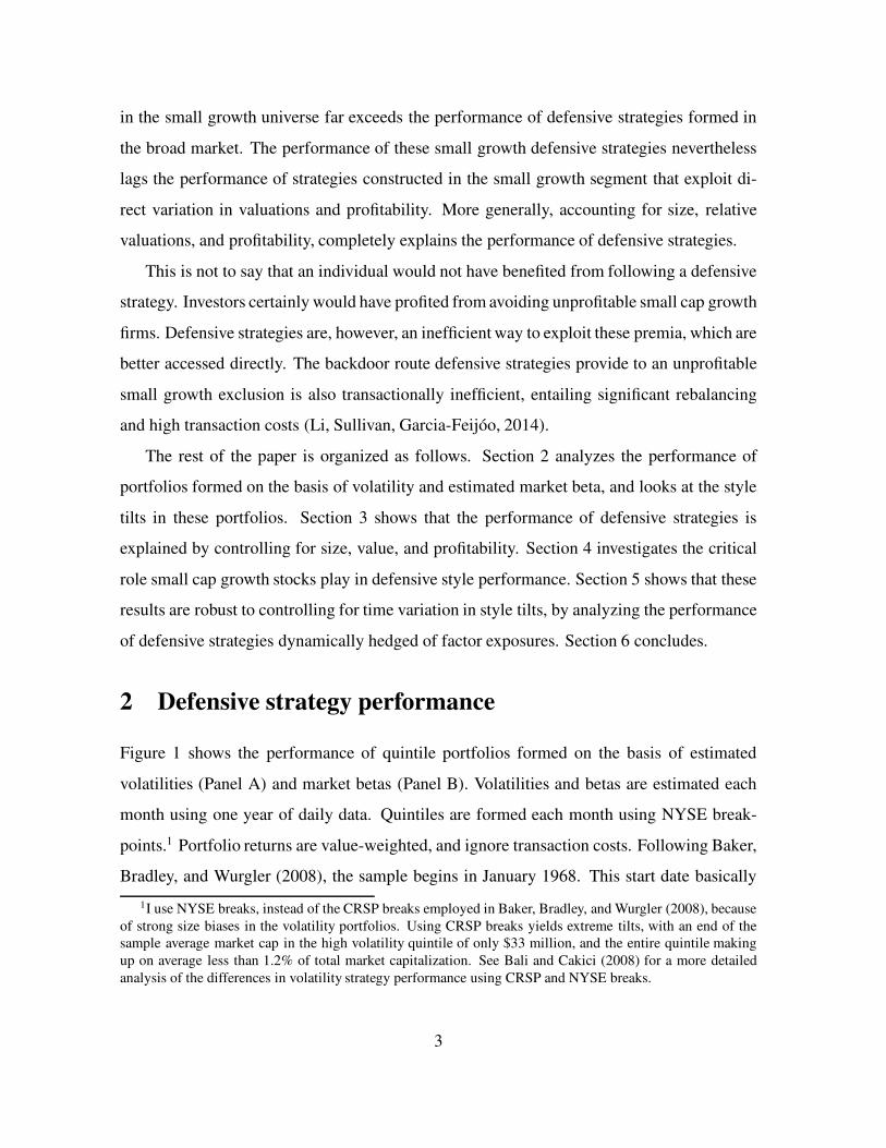
Figure 1 shows the performance of quintile portfolios formed on the basis of estimated

volatilities (Panel A) and market betas (Panel B). Volatilities and betas are estimated each

month using one year of daily data. Quintiles are formed each month using NYSE break-

points.1 Portfolio returns are value-weighted, and ignore transaction costs. Following Baker,

Bradley, and Wurgler (2008), the sample begins in January 1968. This start date basically

1I use NYSE breaks, instead of the CRSP breaks employed in Baker, Bradley, and Wurgler (2008), because

of strong size biases in the volatility portfolios. Using CRSP breaks yields extreme tilts, with an end of thesample average market cap in the high volatility quintile of only $33 million, and the entire quintile making

up on average less than 1.2% of total market capitalization. See Bali and Cakici (2008) for a more detailed

analysis of the differences in volatility strategy performance using CRSP and NYSE breaks.

3

Value of $1 invested in 1968 in volatility portfolios (log scale)

1970 1975 1980 1985 1990 1995 2000 2005 2010

$1

$10

$100

Low vol.

2

3

4

High vol.

Value of $1 invested in 1968 in beta portfolios (log scale)

1970 1975 1980 1985 1990 1995 2000 2005 2010

$1

$10

$100

Low beta

2

3

4

High beta

Figure 1. Performance of volatility and beta quintiles

Growth of $1 invested in quintile portfolios sorted on volatility (top panel) and beta (bottom panel).

Portfolios are rebalanced monthly and ignore transaction costs, and returns are value-weighted. The

sample covers January 1968 through December 2013.

4

coincides with the date at which high volatility stocks began underperforming low volatility

stocks, and thus bias the results toward finding impressive defensive strategy performance

(see Appendix A for pre-1968 performance).

The figure shows that the most aggressive stocks, i.e. those in the high volatility or

high market beta quintile, have dramatically underperformed the rest of the market. This

underperformance is especially pronounced for the high volatility portfolio. In both panels

the figure shows little variation in performance between the other four portfolios, which all

closely track the market.

Figure 2 shows Morningstar-type style boxes for the aggressive and defensive portfolios,

defined using both volatility (Panel A) and market beta (Panel B). Formally the figure shows

log-likelihood ratios that a stock picked at random from one of the defensive or aggressive

volatility or beta portfolios is in particular size and value quintiles (defined using NYSE

breaks), relative to the likelihood that a stock picked at random from the entire universe is

in the same size and value quintiles. That is, the log-likelihood ratio LLRijk that a stock in

risk quintile k is in size quintile i and value quintile j is given by

LLRijk D log

�

P Œslt 2 MEit \ BMjt j slt 2 Rkt �

P Œslt 2 MEit \ BMjt �

�

;

where slt is the stock of a random firm l picked at a random time t , and MEit , BMjt , and

Rkt are market equity quintile i , book-to-market quintile j , and risk quintile k, respectively,

all at time-t . The data underlying the figure are reported in Table 8, in the appendix.

The figure shows strong size and value tilts to the defensive and aggressive portfolios.

These are especially pronounced in the portfolios formed on the basis of volatility. The

left half of Panel A shows a growth tilt, and an extreme tilt toward small caps, for the high

volatility portfolio. The right half shows a strong value tilt, and an extreme tilt toward large

caps, for the low volatility portfolio. Panel B shows a growth tilt to the high beta portfolios,

and small cap and value tilts to the low beta portfolios, though these tilts are less extreme

than those observed on the volatility portfolios.

5

Panel A: Portfolios formed on volatility

High volatility portfolio Low volatility portfolio

Deep value Value Blend Growth High growth

Micro

Small

Mid

Large

Giant

Underweight Overweight


Micro

Small

Mid

Large

Giant


Panel B: Portfolios formed on estimated market betas

High beta portfolio Low beta portfolio


Micro

Small

Mid

Large

Giant



Micro

Small

Mid

Large

Giant


Figure 2. Volatility and beta portfolio style boxes

The figure shows log-likelihood ratios that a randomly selected stock from one of the volatility or beta quintile

portfolios is of a given style (size and value quintile, using NYSE breaks), relative to the unconditional proba-

bility of being that style. The sample covers January 1968 through December 2013. Underlying probabilities

are provided in Table 8 in the appendix.

6

The tilts observed in Figure 2 can also be seen in Tables 1 and 2, which formally ana-

lyze the performance of the volatility and beta portfolios shown in Figure 1. Panel A gives

volatility portfolio characteristics. It does not show significant variation in the time-series

average valuations of the low and high volatility portfolios, but shows enormous variation

in firm size across portfolios. The low volatility stocks are on average more than 25 times

as large as the high volatility stocks at the end of the sample. As a result the high volatil-

ity portfolio on average holds less than nine percent of the market by capitalization, despite

holding almost half of stocks by name. Panel B shows that the average returns across volatil-

ity portfolios are basically flat, or even slightly increasing with volatility, with the exception

of the extremely low returns to the most aggressive stocks. Panel C shows the typical Black,

Jensen, and Scholes (1972) failure of the CAPM, with a significant negative alpha for the

high volatility/high beta portfolio, and a significant positive alpha for the low volatility/low

beta portfolio. Panel D shows results of Fama and French (1993) three-factor regressions us-

ing the volatility portfolio returns, and provides further evidence of the size and value tilts in

the defensive strategies. The long/short strategy has a large value tilt (HML loading of 0.42),

and an enormous large cap tilt (SMB loading of -1.12). Despite the highly significant factor

loadings, the three-factor model is unable to price the defensive strategy, which generates

three-factor abnormal returns of 68 basis points per month (t-stat of 4.29). Five-sixths of this

alpha (57 out of 68 bps/month) is delivered, however, by the aggressive stocks on the short

side of the strategy, with only one-sixth, or eleven basis points per month, coming from the

actual defensive stocks.

Table 2 shows similar, though less challenging, results for the portfolios sorted on esti-

mated market betas. The table provides evidence of larger value tilts, though smaller size

tilts, to the beta portfolios. It also shows that while the anti-beta strategy generates a sig-

nificant CAPM alpha, it does not deliver significant abnormal returns after controlling for

exposures to the size and value factors. Because the volatility strategies present a challenge

to the standard three-factor model while the beta strategies do not, the remainder of the paper

focuses on the former, relegating test results for beta strategies to the appendix.

7

Table 1. Volatility portfolio performance

The table reports time-series average characteristics (Panel A), monthly average excess returns (Panel B), and

results of time-series regressions using the CAPM and the Fama and French three-factor model (Panels C and

D, respectively), of quintile portfolios sorted on volatility. Portfolios are rebalanced monthly using NYSE

breaks. Returns are value-weighted, and ignore transaction costs. The sample includes all NYSE, NASDAQ,

and AMEX common stocks, and covers January 1968 through December 2013.

Volatility quintiles

(H) (2) (3) (4) (L) (L-H)

Panel A: Portfolio characteristics

Firms (%) 49.5 15.5 11.5 9.99 13.5

Cap. (%) 8.6 10.7 16.7 25.7 38.3

B/M 0.65 0.63 0.63 0.60 0.65

ME2013 ($106) 84 204 709 931 2,209

Panel B: Portfolio average monthly excess returns

E[Re] 0.19 0.59 0.57 0.55 0.52 0.33[0.53] [2.14] [2.46] [2.83] [3.44] [1.13]

Panel C: CAPM regression results

˛ -0.59 -0.05 0.03 0.10 0.19 0.78[-3.52] [-0.60] [0.42] [1.57] [2.77] [3.52]

ˇMKT 1.63 1.34 1.14 0.94 0.68 -0.95[45.0] [72.3] [78.0] [67.7] [46.3] [-19.8]

Adj.-R2 (%) 78.6 90.5 91.7 89.3 79.6 41.6

Panel D: Three-factor model regression results

˛ -0.57 -0.11 -0.04 0.03 0.11 0.68[-4.69] [-1.40] [-0.57] [0.47] [2.02] [4.29]

ˇMKT 1.41 1.28 1.17 1.02 0.78 -0.63[50.5] [73.1] [75.6] [79.4] [61.5] [-17.4]

ˇSMB 0.88 0.34 -0.01 -0.18 -0.24 -1.12[22.1] [13.5] [-0.28] [-9.72] [-13.3] [-21.5]

ˇHML -0.21 0.05 0.14 0.19 0.21 0.42[-5.05] [1.86] [5.80] [9.62] [10.7] [7.59]

Adj.-R2 (%) 89.4 92.9 92.2 92.4 87.5 71.7

8

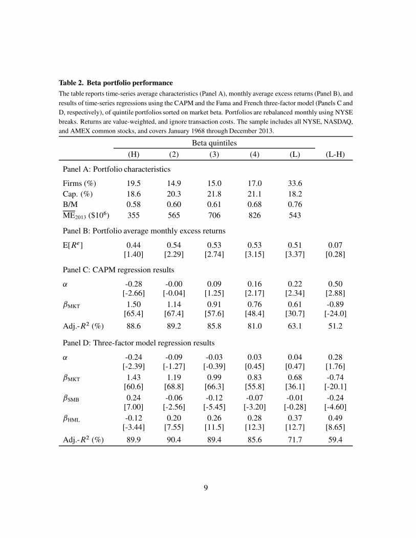
Table 2. Beta portfolio performance

The table reports time-series average characteristics (Panel A), monthly average excess returns (Panel B), and

results of time-series regressions using the CAPM and the Fama and French three-factor model (Panels C and

D, respectively), of quintile portfolios sorted on market beta. Portfolios are rebalanced monthly using NYSE

breaks. Returns are value-weighted, and ignore transaction costs. The sample includes all NYSE, NASDAQ,

and AMEX common stocks, and covers January 1968 through December 2013.

Beta quintiles

(H) (2) (3) (4) (L) (L-H)


Firms (%) 19.5 14.9 15.0 17.0 33.6

Cap. (%) 18.6 20.3 21.8 21.1 18.2

B/M 0.58 0.60 0.61 0.68 0.76

ME2013 ($106) 355 565 706 826 543


E[Re] 0.44 0.54 0.53 0.53 0.51 0.07[1.40] [2.29] [2.74] [3.15] [3.37] [0.28]


˛ -0.28 -0.00 0.09 0.16 0.22 0.50[-2.66] [-0.04] [1.25] [2.17] [2.34] [2.88]

ˇMKT 1.50 1.14 0.91 0.76 0.61 -0.89[65.4] [67.4] [57.6] [48.4] [30.7] [-24.0]

Adj.-R2 (%) 88.6 89.2 85.8 81.0 63.1 51.2


˛ -0.24 -0.09 -0.03 0.03 0.04 0.28[-2.39] [-1.27] [-0.39] [0.45] [0.47] [1.76]

ˇMKT 1.43 1.19 0.99 0.83 0.68 -0.74[60.6] [68.8] [66.3] [55.8] [36.1] [-20.1]

ˇSMB 0.24 -0.06 -0.12 -0.07 -0.01 -0.24[7.00] [-2.56] [-5.45] [-3.20] [-0.28] [-4.60]

ˇHML -0.12 0.20 0.26 0.28 0.37 0.49[-3.44] [7.55] [11.5] [12.3] [12.7] [8.65]

Adj.-R2 (%) 89.9 90.4 89.4 85.6 71.7 59.4

9

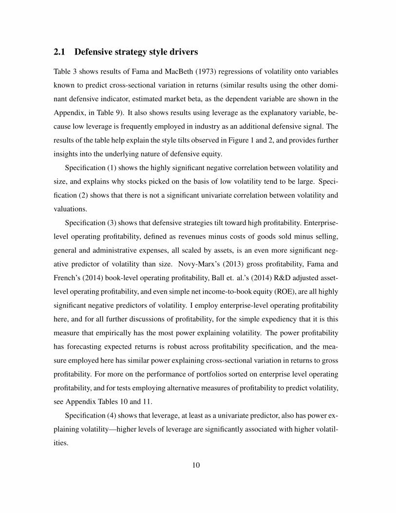
2.1 Defensive strategy style drivers

Table 3 shows results of Fama and MacBeth (1973) regressions of volatility onto variables

known to predict cross-sectional variation in returns (similar results using the other domi-

nant defensive indicator, estimated market beta, as the dependent variable are shown in the

Appendix, in Table 9). It also shows results using leverage as the explanatory variable, be-

cause low leverage is frequently employed in industry as an additional defensive signal. The

results of the table help explain the style tilts observed in Figure 1 and 2, and provides further

insights into the underlying nature of defensive equity.

Specification (1) shows the highly significant negative correlation between volatility and

size, and explains why stocks picked on the basis of low volatility tend to be large. Speci-

fication (2) shows that there is not a significant univariate correlation between volatility and

valuations.

Specification (3) shows that defensive strategies tilt toward high profitability. Enterprise-

level operating profitability, defined as revenues minus costs of goods sold minus selling,

general and administrative expenses, all scaled by assets, is an even more significant neg-

ative predictor of volatility than size. Novy-Marx’s (2013) gross profitability, Fama and

French’s (2014) book-level operating profitability, Ball et. al.’s (2014) R&D adjusted asset-

level operating profitability, and even simple net income-to-book equity (ROE), are all highly

significant negative predictors of volatility. I employ enterprise-level operating profitability

here, and for all further discussions of profitability, for the simple expediency that it is this

measure that empirically has the most power explaining volatility. The power profitability

has forecasting expected returns is robust across profitability specification, and the mea-

sure employed here has similar power explaining cross-sectional variation in returns to gross

profitability. For more on the performance of portfolios sorted on enterprise level operating

profitability, and for tests employing alternative measures of profitability to predict volatility,

see Appendix Tables 10 and 11.

Specification (4) shows that leverage, at least as a univariate predictor, also has power ex-

plaining volatility—higher levels of leverage are significantly associated with higher volatil-

ities.

10

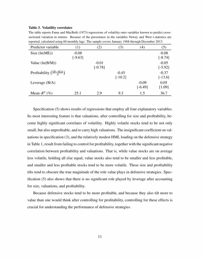
Table 3. Volatility correlates

The table reports Fama and MacBeth (1973) regressions of volatility onto variables known to predict cross-

sectional variation in returns. Because of the persistence in the variables Newey and West t-statistics are

reported, calculated using 60 monthly lags. The sample covers January 1968 through December 2013.

Predictor variable (1) (2) (3) (4) (5)

Size (ln(ME)) -0.08 -0.08[-9.63] [-8.74]

Value (ln(B/M)) -0.01 -0.05[-0.78] [-5.92]

Profitability�

GP�SGAA

�

-0.45 -0.37[-10.2] [-13.6]

Leverage (B/A) -0.09 0.05[-6.49] [1.09]

Mean-R2 (%) 25.1 2.9 9.3 1.5 36.7

Specification (5) shows results of regressions that employ all four explanatory variables.

Its most interesting feature is that valuations, after controlling for size and profitability, be-

come highly significant correlates of volatility. Highly volatile stocks tend to be not only

small, but also unprofitable, and to carry high valuations. The insignificant coefficient on val-

uations in specification (3), and the relatively modest HML loading on the defensive strategy

in Table 1, result from failing to control for profitability, together with the significant negative

correlation between profitability and valuations. That is, while value stocks are on average

less volatile, holding all else equal, value stocks also tend to be smaller and less profitable,

and smaller and less profitable stocks tend to be more volatile. These size and profitability

tilts tend to obscure the true magnitude of the role value plays in defensive strategies. Spec-

ification (5) also shows that there is no significant role played by leverage after accounting

for size, valuations, and profitability.

Because defensive stocks tend to be more profitable, and because they also tilt more to

value than one would think after controlling for profitability, controlling for these effects is

crucial for understanding the performance of defensive strategies.

11

3 Defensive strategy performance controlling for size

Controlling for size is critical when analyzing strategies based on volatility, because the size

biases observed in the unconditional sorts on volatility (Table 1) are particularly extreme.

The size bias also interacts with value, which has experienced much stronger performance

among small cap stocks. Table 4 controls for size by constructing defensive strategies within

size universes.2

At the start of each month firms are assigned to size portfolios, defined by NYSE market

cap deciles (size portfolios characteristics provided in Panel A of Table 4). Within each size

decile a defensive-minus-aggressive (DMA) strategy is formed, by buying (selling) the 30%

of stocks with the lowest (highest) estimated volatility. Returns are again value-weighted,

and ignore transaction costs.3 Panel B of Table 4 shows that the average monthly excess

returns to the ten DMA strategies was almost 50 basis points per month. While this per-

formance was somewhat concentrated in the lowest three size deciles, which make up on

average just 5.4 percent of the market by capitalization, performance was positive in every

size decile, and a Gibbons, Ross, and Shanken (GRS, 1989) test rejects the null that the

excess returns are jointly zero at the one percent level. Panel C shows that the strategies

on average have loadings of -0.84 on the market, leading to all ten strategies having highly

significant CAPM alphas, which average 90 basis points per month.

Panel D shows that the Fama and French model explains much more of the strategies’

return variation than the CAPM, an average of 61.4% compared to 36.1%, but explains less

than a third of the strategies’ average returns. The three factor model has some success

pricing the defensive strategies in the three largest size deciles, which make up on average

80% of the market by capitalization, but even among these large cap stocks the defensive

strategies deliver positive, though insignificant, abnormal returns.

2Controlling for size is equally important when analyzing strategies based on market beta. For example, thesignal weighting procedure employed by Frazzini and Pedersen (2014), which overweights small stocks even

more than an equal-weighting scheme, is a crucial driver of the performance of their beta-based BAB factor.

Results of tests similar to those presented in Table 4, using defensive strategies constructed within size deciles

on the basis of estimated market beta instead of volatility, are provide in the Appendix in Table 12.3I use the top and bottom 30% when constructing these strategies inside the size portfolios. The largest size

deciles contain only about 200 names at the end of the sample, and even fewer in the early sample. A more

extreme second sort consequence yields poorly diversified strategies.

12

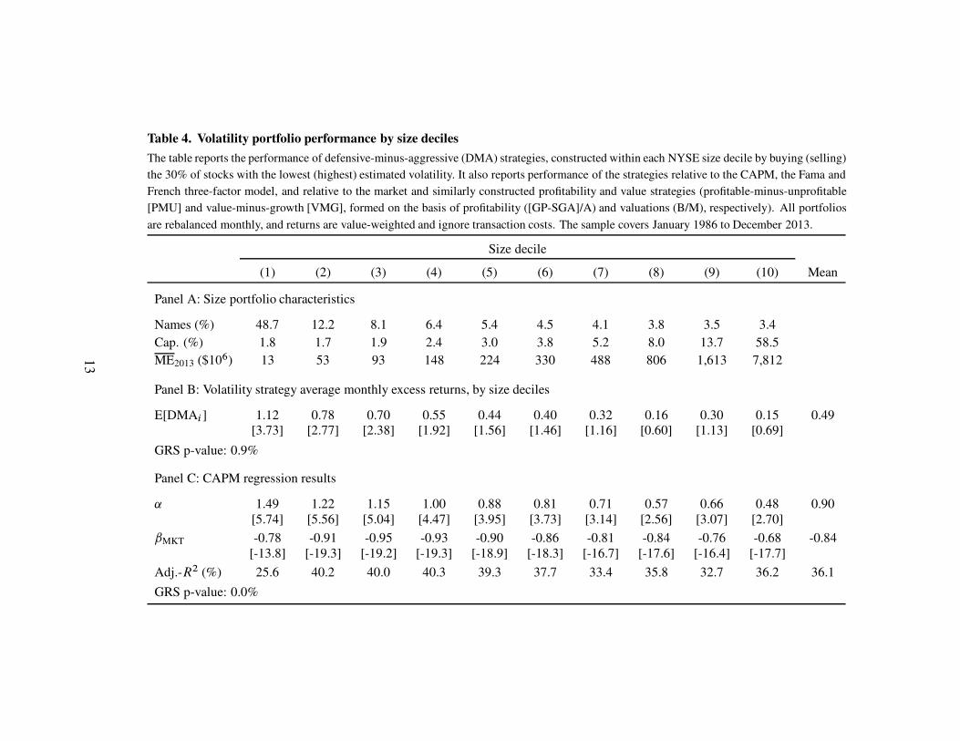
Table 4. Volatility portfolio performance by size deciles

The table reports the performance of defensive-minus-aggressive (DMA) strategies, constructed within each NYSE size decile by buying (selling)

the 30% of stocks with the lowest (highest) estimated volatility. It also reports performance of the strategies relative to the CAPM, the Fama and

French three-factor model, and relative to the market and similarly constructed profitability and value strategies (profitable-minus-unprofitable

[PMU] and value-minus-growth [VMG], formed on the basis of profitability ([GP-SGA]/A) and valuations (B/M), respectively). All portfolios

are rebalanced monthly, and returns are value-weighted and ignore transaction costs. The sample covers January 1986 to December 2013.

Size decile

(1) (2) (3) (4) (5) (6) (7) (8) (9) (10) Mean

Panel A: Size portfolio characteristics

Names (%) 48.7 12.2 8.1 6.4 5.4 4.5 4.1 3.8 3.5 3.4

Cap. (%) 1.8 1.7 1.9 2.4 3.0 3.8 5.2 8.0 13.7 58.5

ME2013 ($106) 13 53 93 148 224 330 488 806 1,613 7,812

Panel B: Volatility strategy average monthly excess returns, by size deciles

E[DMAi ] 1.12 0.78 0.70 0.55 0.44 0.40 0.32 0.16 0.30 0.15 0.49[3.73] [2.77] [2.38] [1.92] [1.56] [1.46] [1.16] [0.60] [1.13] [0.69]

GRS p-value: 0.9%


˛ 1.49 1.22 1.15 1.00 0.88 0.81 0.71 0.57 0.66 0.48 0.90[5.74] [5.56] [5.04] [4.47] [3.95] [3.73] [3.14] [2.56] [3.07] [2.70]

ˇMKT -0.78 -0.91 -0.95 -0.93 -0.90 -0.86 -0.81 -0.84 -0.76 -0.68 -0.84[-13.8] [-19.3] [-19.2] [-19.3] [-18.9] [-18.3] [-16.7] [-17.6] [-16.4] [-17.7]

Adj.-R2 (%) 25.6 40.2 40.0 40.3 39.3 37.7 33.4 35.8 32.7 36.2 36.1

GRS p-value: 0.0%

13

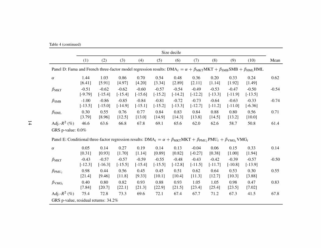
Table 4 (continued)

Size decile

(1) (2) (3) (4) (5) (6) (7) (8) (9) (10) Mean

Panel D: Fama and French three-factor model regression results: DMAi D ˛ C ˇMKTMKT C ˇSMBSMB C ˇHMLHML

˛ 1.44 1.03 0.86 0.70 0.54 0.48 0.36 0.20 0.33 0.24 0.62[6.41] [5.91] [4.97] [4.20] [3.34] [2.89] [2.11] [1.14] [1.92] [1.49]

ˇMKT -0.51 -0.62 -0.62 -0.60 -0.57 -0.54 -0.49 -0.53 -0.47 -0.50 -0.54[-9.79] [-15.4] [-15.4] [-15.6] [-15.2] [-14.2] [-12.2] [-13.3] [-11.9] [-13.5]

ˇSMB -1.00 -0.86 -0.85 -0.84 -0.81 -0.72 -0.73 -0.64 -0.63 -0.33 -0.74[-13.5] [-15.0] [-14.9] [-15.1] [-15.2] [-13.3] [-12.7] [-11.2] [-11.0] [-6.36]

ˇHML 0.30 0.55 0.76 0.77 0.84 0.83 0.84 0.88 0.80 0.56 0.71[3.79] [8.96] [12.5] [13.0] [14.9] [14.3] [13.8] [14.5] [13.2] [10.0]

Adj.-R2 (%) 46.6 63.6 66.8 67.8 69.1 65.6 62.0 62.6 58.7 50.8 61.4

GRS p-value: 0.0%

Panel E: Conditional three-factor regression results: DMAi D ˛ C ˇMKTMKT C ˇPMUiPMUi C ˇVMGi

VMGi

˛ 0.05 0.14 0.27 0.19 0.14 0.13 -0.04 0.06 0.15 0.33 0.14[0.31] [0.93] [1.70] [1.14] [0.89] [0.82] [-0.27] [0.38] [1.00] [1.94]

ˇMKT -0.43 -0.57 -0.57 -0.59 -0.55 -0.48 -0.43 -0.42 -0.39 -0.57 -0.50[-12.3] [-16.3] [-15.5] [-15.4] [-15.5] [-12.8] [-11.5] [-11.7] [-10.8] [-13.9]

ˇPMUi0.98 0.44 0.56 0.45 0.45 0.51 0.62 0.64 0.53 0.30 0.55

[21.4] [9.46] [11.8] [9.33] [10.1] [10.4] [11.3] [12.7] [10.3] [3.88]

ˇVMGi0.40 0.80 0.82 0.93 0.88 0.93 1.05 1.05 0.98 0.47 0.83

[7.84] [20.7] [22.1] [21.3] [22.9] [21.5] [23.4] [25.4] [23.5] [7.02]

Adj.-R2 (%) 75.4 72.8 73.3 69.6 72.1 67.4 67.7 71.2 67.3 41.5 67.8

GRS p-value, residual returns: 34.2%

14

Panel E compares the performance of the defensive strategies constructed within size

deciles to the performance of similarly constructed profitability and value strategies. These

profitable-minus-unprofitable (PMU) and value-minus-growth (VMG) strategies are formed

using the same methodology as the defensive strategies, but the positions in each strategy are

selected on the basis of profitability ([GP-SGA]/A) or valuations (B/M) instead of volatil-

ity. None of the defensive strategies yield significant abnormal returns relative to similarly

constructed profitability and value strategies, even after accounting for the hedge they pro-

vide for the market. All of the defensive strategies have highly significant positive loadings

on profitability, and accounting for profitability increases the strategies’ loadings on value.

As a result of these large profitability and value loadings, none of the defensive strategies

generates significant abnormal returns, despite having market betas averaging -0.50. A GRS

test fails to reject that the three-factor residual returns to the ten strategies are jointly zero

(p-value of 34.2%).

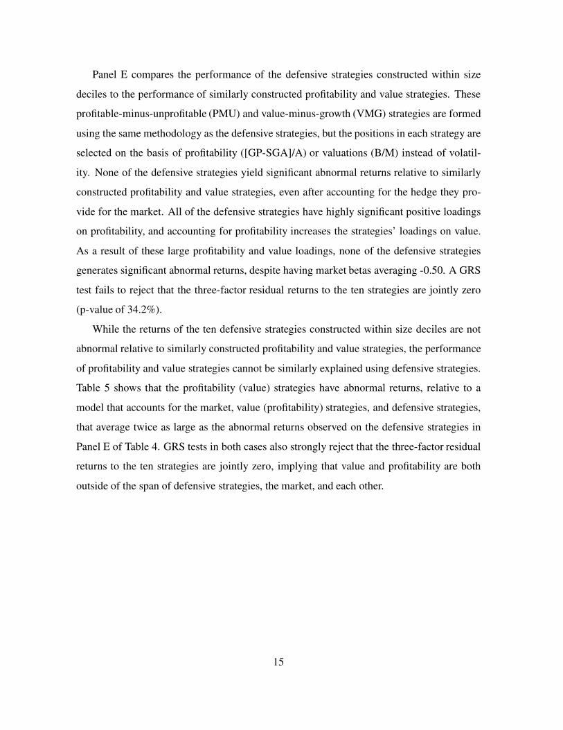
While the returns of the ten defensive strategies constructed within size deciles are not

abnormal relative to similarly constructed profitability and value strategies, the performance

of profitability and value strategies cannot be similarly explained using defensive strategies.

Table 5 shows that the profitability (value) strategies have abnormal returns, relative to a

model that accounts for the market, value (profitability) strategies, and defensive strategies,

that average twice as large as the abnormal returns observed on the defensive strategies in

Panel E of Table 4. GRS tests in both cases also strongly reject that the three-factor residual

returns to the ten strategies are jointly zero, implying that value and profitability are both

outside of the span of defensive strategies, the market, and each other.

15

Table 5. Spanning tests of value, profitability, and volatility-based defensive strategies, constructed within size deciles

The table reports the performance of value-minus-growth (VMG) and profitable-minus-unprofitable (PMU) strategies, constructed within each

NYSE size decile by buying (selling) the 30% of stocks with the lowest (highest) valuations (B/M) and profitability ([GP-SGA]/A), respectively.

It also reports performance of both sets of strategies relative to the market, each other, and similarly constructed defensive strategies (defensive-

minus-aggressive [DFA], defined using estimated volatility). All portfolios are rebalanced monthly, and returns are value-weighted and ignore

transaction costs. The sample covers January 1986 to December 2013.

Size decile

(1) (2) (3) (4) (5) (6) (7) (8) (9) (10) Mean

Panel A: Value strategy average monthly excess returns, by size deciles

E[VMGi ] 0.99 0.82 0.57 0.43 0.51 0.44 0.38 0.15 0.24 0.11 0.46[5.90] [4.42] [2.95] [2.55] [2.81] [2.54] [2.36] [0.91] [1.45] [0.71]

GRS p-value: 0.0%

Panel B: Conditional three-factor regression results: VMGi D ˛ C ˇMKTMKT C ˇPMUiPMUi C ˇDMAi

DMAi

˛ 0.54 0.37 0.23 0.25 0.27 0.29 0.33 0.16 0.15 0.26 0.28[4.39] [2.94] [1.75] [2.13] [2.20] [2.52] [3.07] [1.49] [1.34] [2.50]

ˇMKT -0.09 0.11 0.10 0.09 0.12 0.03 0.04 0.05 0.03 -0.13 0.04[-2.75] [3.22] [2.79] [2.62] [3.57] [1.11] [1.52] [1.76] [1.05] [-4.48]

ˇPMUi0.24 -0.07 -0.25 -0.23 -0.22 -0.37 -0.44 -0.48 -0.40 -0.80 -0.30

[4.86] [-1.75] [-5.81] [-6.45] [-6.03] [-10.4] [-11.9] [-14.0] [-10.9] [-23.9]

ˇDMAi0.25 0.55 0.57 0.49 0.55 0.49 0.48 0.51 0.51 0.17 0.46

[7.84] [20.7] [22.1] [21.3] [22.9] [21.5] [23.4] [25.4] [23.5] [7.02]

Adj.-R2 (%) 50.5 56.0 57.3 54.6 56.9 56.2 58.3 62.9 58.3 54.9 56.6


16

Table 5 (continued)

Size decile

(1) (2) (3) (4) (5) (6) (7) (8) (9) (10) Mean

Panel C: Profitability strategy average monthly excess returns, by size deciles

E[PMUi ] 0.90 0.60 0.42 0.54 0.27 0.19 0.27 0.23 0.18 0.15 0.37[5.07] [4.26] [3.06] [3.85] [1.89] [1.34] [2.12] [1.72] [1.36] [1.10]

GRS p-value: 0.0%

Panel D: Conditional three-factor regression results: PMUi D ˛ C ˇMKTMKT C ˇPMUiVMGi C ˇDMAi

DMAi

˛ 0.11 0.32 0.21 0.43 0.19 0.23 0.36 0.26 0.22 0.28 0.26[1.00] [2.47] [1.66] [3.19] [1.41] [1.85] [3.21] [2.33] [1.89] [3.07]

ˇMKT 0.20 0.18 0.19 0.16 0.14 0.03 -0.01 -0.01 -0.05 -0.17 0.07[7.79] [5.15] [5.60] [4.32] [3.84] [0.95] [-0.36] [-0.35] [-1.60] [-6.89]

ˇDMAi0.46 0.32 0.36 0.30 0.35 0.32 0.30 0.36 0.31 0.09 0.32

[21.4] [9.46] [11.8] [9.33] [10.1] [10.4] [11.3] [12.7] [10.3] [3.88]

ˇVMGi0.18 -0.08 -0.23 -0.30 -0.28 -0.44 -0.47 -0.55 -0.45 -0.64 -0.33

[4.86] [-1.75] [-5.81] [-6.45] [-6.03] [-10.4] [-11.9] [-14.0] [-10.9] [-23.9]

Adj.-R2 (%) 66.7 20.0 21.1 13.3 16.0 20.4 25.4 31.2 23.6 53.3 29.1


17

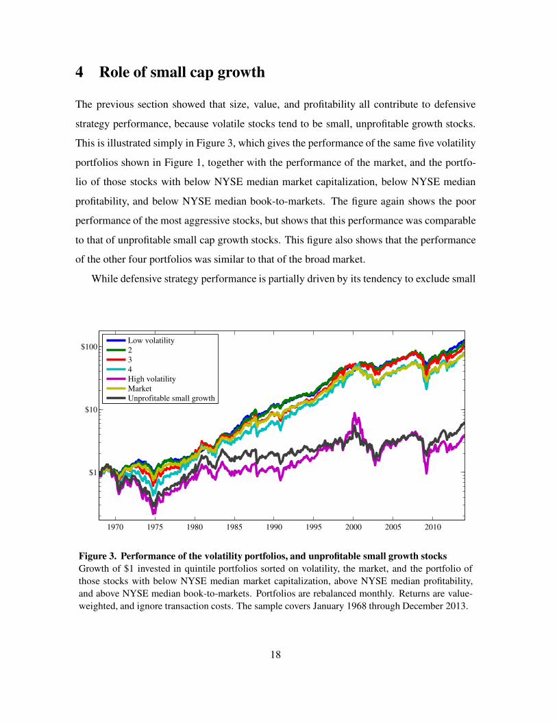
4 Role of small cap growth

The previous section showed that size, value, and profitability all contribute to defensive

strategy performance, because volatile stocks tend to be small, unprofitable growth stocks.

This is illustrated simply in Figure 3, which gives the performance of the same five volatility

portfolios shown in Figure 1, together with the performance of the market, and the portfo-

lio of those stocks with below NYSE median market capitalization, below NYSE median

profitability, and below NYSE median book-to-markets. The figure again shows the poor

performance of the most aggressive stocks, but shows that this performance was comparable

to that of unprofitable small cap growth stocks. This figure also shows that the performance

of the other four portfolios was similar to that of the broad market.

While defensive strategy performance is partially driven by its tendency to exclude small

Value of $1 invested in 1968

1970 1975 1980 1985 1990 1995 2000 2005 2010

$1

$10

$100

Low volatility234High volatilityMarketUnprofitable small growth

Figure 3. Performance of the volatility portfolios, and unprofitable small growth stocks

Growth of $1 invested in quintile portfolios sorted on volatility, the market, and the portfolio of

those stocks with below NYSE median market capitalization, above NYSE median profitability,

and above NYSE median book-to-markets. Portfolios are rebalanced monthly. Returns are value-

weighted, and ignore transaction costs. The sample covers January 1968 through December 2013.

18

cap growth stocks, small cap growth plays an important additional, indirect role in the per-

formance of defensive strategies. While the previous section shows defensive performance

is stronger among smaller stocks, this section shows that defensive performance is, after

controlling for style, wholly concentrated in the small cap growth sector.

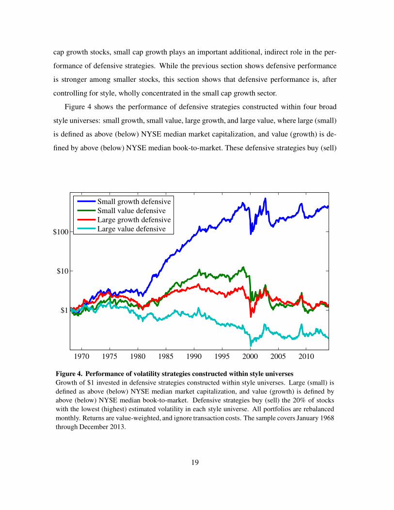
Figure 4 shows the performance of defensive strategies constructed within four broad

style universes: small growth, small value, large growth, and large value, where large (small)

is defined as above (below) NYSE median market capitalization, and value (growth) is de-

fined by above (below) NYSE median book-to-market. These defensive strategies buy (sell)

Value of $1 invested in 1968 (log scale)

1970 1975 1980 1985 1990 1995 2000 2005 2010

$1

$10

$100

Small growth defensiveSmall value defensiveLarge growth defensiveLarge value defensive

Figure 4. Performance of volatility strategies constructed within style universes

Growth of $1 invested in defensive strategies constructed within style universes. Large (small) is

defined as above (below) NYSE median market capitalization, and value (growth) is defined by

above (below) NYSE median book-to-market. Defensive strategies buy (sell) the 20% of stocks

with the lowest (highest) estimated volatility in each style universe. All portfolios are rebalanced

monthly. Returns are value-weighted, and ignore transaction costs. The sample covers January 1968

through December 2013.

19

the 20% of stocks with the lowest (highest) estimated volatility in each style universe. Port-

folios are rebalanced monthly. Returns are value-weighted and ignore transaction costs. The

sample again covers January 1968 to December 2013.

The figure shows that $1 invested in the beginning of 1968 in the defensive strategy con-

structed within small cap growth, a segment that accounts for on average 38.0% of names but

only 5.4% of the market by capitalization, would have grown to $429, ignoring transaction

costs, by the end of 2013. That same dollar invested in defensive strategies constructed in

the small cap value or large cap growth universes would have grown to only $1.22 or $1.34,

respectively, a period over which a dollar invested in T-bills grew to $10.30. That same dollar

invested into a defensive strategy constructed using large cap value stocks would have left

the investor with only $0.18 by the end of 2013, an 82% loss of capital over the sample.

In order to understand why the small growth defensive strategy performed so well, it is

useful to look at the characteristics of the volatility portfolios within the small growth sector.

Time-series average characteristics for these portfolios are reported in Table 6. The table

shows extreme valuations and profitabilities for the most volatile small growth stocks. These

volatile stocks are on average less than a third as large as the typical small growth stock. The

entire portfolio also has negative book equity, negative earnings, and operating profitability

less than one fifth that of the next highest volatility portfolio. The large differences in returns

between the most and least volatile small growth stocks results from this extreme variation

Table 6. Small growth volatility portfolio characteristics

The table reports time-series average characteristics of quintile portfolios sorted on volatility, restricted to

stocks with below average NYSE median market capitalizations and book-to-markets. The sample covers

Jauary 1968 to December 2013.

Volatility quintile decile

(H) (4) (3) (2) (L)

Firm size ($106) 55 120 184 239 299

Valuation (B/M) -0.21 0.30 0.37 0.41 0.49

Return-on-market equity (NI/M) -43.3% -4.3% 2.3% 4.9% 6.6%

Operating profitability�

GP�SGAA

�

1.4% 7.7% 11.8% 13.4% 9.8%

20

in valuations and profitabilities. In the other sectors, where defensive stocks do not signifi-

cantly outperform aggressive stocks, sorting on volatility yields little variation in operating

profitability, and in the value sectors the defensive strategies actually tilt to growth, not value.

The extreme variation in valuations and profitabilities that result from sorting small

growth stocks on the basis of volatility can only arise, however, because of the extreme vari-

ation in these characteristics that exists in this segment, and this variation can just as easily

be exploited directly. In fact, Table 7 shows that the small growth defensive strategies’ im-

pressive performance was completely unremarkable after controlling for the strategy’s value

and profitability tilts. The first specification shows that the small growth defensive strategy

generated excess returns of more than 1.5% per month. The second and third specifications

show even larger CAPM and Fama and French three-factor alphas, both significant with t-

stats of six. The fourth specification shows that the small growth defensive strategy’s returns

are completely explained by the market and small growth profitability and value factors.

The fifth specification shows similar results using a two-factor model employing the market

and the returns to a strategy that buys (sells) small growth stocks with above (below) both

segment median operating profitability and book-to-market.

Figure 5 shows the performance of the small growth defensive strategy, together with the

performance of the three-and two-factor replicating portfolios from specifications (4) and

(5) of the previous table. The three-factor replicating portfolio holds $1.29 of T-bills, and

$0.73 and $0.87 of the small growth stocks with the highest operating profitabilities and

book-to-markets, respectively, while shorting $0.29 of the market and $0.73 and $0.87 of the

small growth stocks with the lowest operating profitabilities and book-to-markets, respec-

tively. The two-factor replicating portfolio holds $1.32 of T-bills and $1.46 of small growth

stocks with both above segment median operating profitabilities and book-to-markets, while

shorting $0.32 of the market and $1.46 of small growth stocks with both below segment

median operating profitabilities and book-to-markets. The figure shows that over the 46 year

sample $1 invested in the small growth defensive strategy instead of the three- or two-factor

replicating portfolios would have grown less ($429, vs. $560 and $1,015), and subjected the

investor to more volatility (28.8%, vs. 24.3% and 24.7%).

21

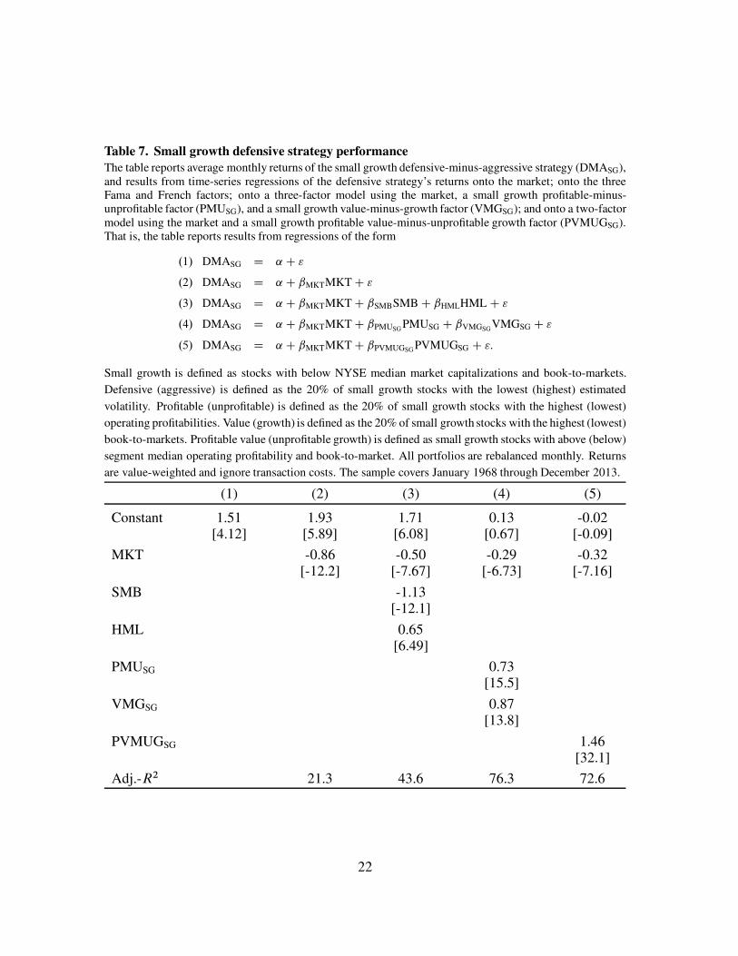
Table 7. Small growth defensive strategy performance

The table reports average monthly returns of the small growth defensive-minus-aggressive strategy (DMASG),and results from time-series regressions of the defensive strategy’s returns onto the market; onto the threeFama and French factors; onto a three-factor model using the market, a small growth profitable-minus-unprofitable factor (PMUSG), and a small growth value-minus-growth factor (VMGSG); and onto a two-factormodel using the market and a small growth profitable value-minus-unprofitable growth factor (PVMUGSG).That is, the table reports results from regressions of the form

.1/ DMASG D ˛ C "

.2/ DMASG D ˛ C ˇMKTMKT C "

.3/ DMASG D ˛ C ˇMKTMKT C ˇSMBSMB C ˇHMLHML C "

.4/ DMASG D ˛ C ˇMKTMKT C ˇPMUSGPMUSG C ˇVMGSG

VMGSG C "

.5/ DMASG D ˛ C ˇMKTMKT C ˇPVMUGSG PVMUGSG C ":

Small growth is defined as stocks with below NYSE median market capitalizations and book-to-markets.

Defensive (aggressive) is defined as the 20% of small growth stocks with the lowest (highest) estimated

volatility. Profitable (unprofitable) is defined as the 20% of small growth stocks with the highest (lowest)

operating profitabilities. Value (growth) is defined as the 20% of small growth stocks with the highest (lowest)

book-to-markets. Profitable value (unprofitable growth) is defined as small growth stocks with above (below)

segment median operating profitability and book-to-market. All portfolios are rebalanced monthly. Returns

are value-weighted and ignore transaction costs. The sample covers January 1968 through December 2013.

(1) (2) (3) (4) (5)

Constant 1.51 1.93 1.71 0.13 -0.02[4.12] [5.89] [6.08] [0.67] [-0.09]

MKT -0.86 -0.50 -0.29 -0.32[-12.2] [-7.67] [-6.73] [-7.16]

SMB -1.13[-12.1]

HML 0.65[6.49]

PMUSG 0.73[15.5]

VMGSG 0.87[13.8]

PVMUGSG 1.46[32.1]

Adj.-R2 21.3 43.6 76.3 72.6

22

Value of $1 invested in 1968 (log scale)

1970 1975 1980 1985 1990 1995 2000 2005 2010

$1

$10

$100

$1,000

Small growth defensive

Three−factor replicating portfolio

Two−factor replicating portfolio

Figure 5. Performance of the small growth defensive strategy, and replicating portfolios based

on profitability and value

Growth of $1 invested in the small growth defensive strategy, and replicating strategies that buy

(sell) small growth stocks with relatively high (low) profitabilities and book-to-markets. Large

(small) is defined as above (below) NYSE median market capitalization, and value (growth) is

defined by above (below) NYSE median book-to-market. The small growth defensive strategy buys

(sells) the 20% of stocks with the lowest (highest) estimated volatility in the small growth segment.

The three-factor replicating portfolio uses the market, a factor that buys (sells) the 20% of stocks

with the highest (lowest) operating profitabilities in the small growth segment, and a factor that buys

(sells) the 20% of stocks with the highest (lowest) book-to-markets in the small growth segment.

The two-factor replicating portfolio uses the market and factor that buys (sells) small growth stocks

with above (below) both segment median operating profitability book-to-market. All portfolios are

rebalanced monthly. Returns are value-weighted and ignore transaction costs. The sample covers

January 1968 through December 2013.

23

5 Dynamic hedging

Some of the best known defensive strategies, such as Frazzini and Pedersen’s (2014) betting-

against-beta strategy, are actively managed in order to keep the strategies close to beta-

neutral. This suggests the possibility that time-variation in factor exposures, and proper

timing to exploit these factors’ associated premia, could be important for defensive strategy

performance.

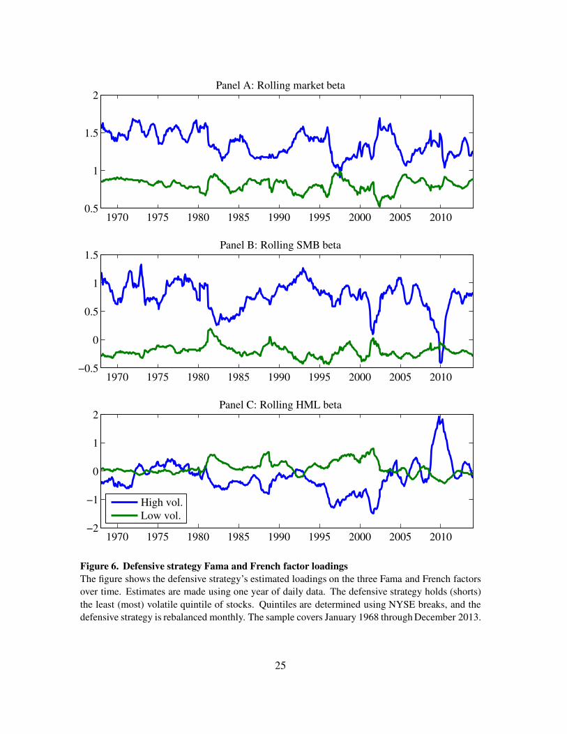
Figure 6 shows that defensive (low volatility) and aggressive (high volatility) stocks do

have important time-variation in their exposures to the Fama and French factors. Panel A

shows the large average spread between aggressive and defensive stocks’ market loadings,

but shows that this spread was more variable later in the sample. Panel B shows the extreme

average spread between aggressive and defensive stocks’ SMB loadings, but also shows

sharp contractions in this spread around the bear markets of the early 1980’s, the early 2000’s,

and especially during the more recent great recession, when the spread actually briefly turned

negative. Panel C shows the defensive stocks’ higher average HML loadings, but shows

much more variation in the spread between defensive and aggressive stocks than for the other

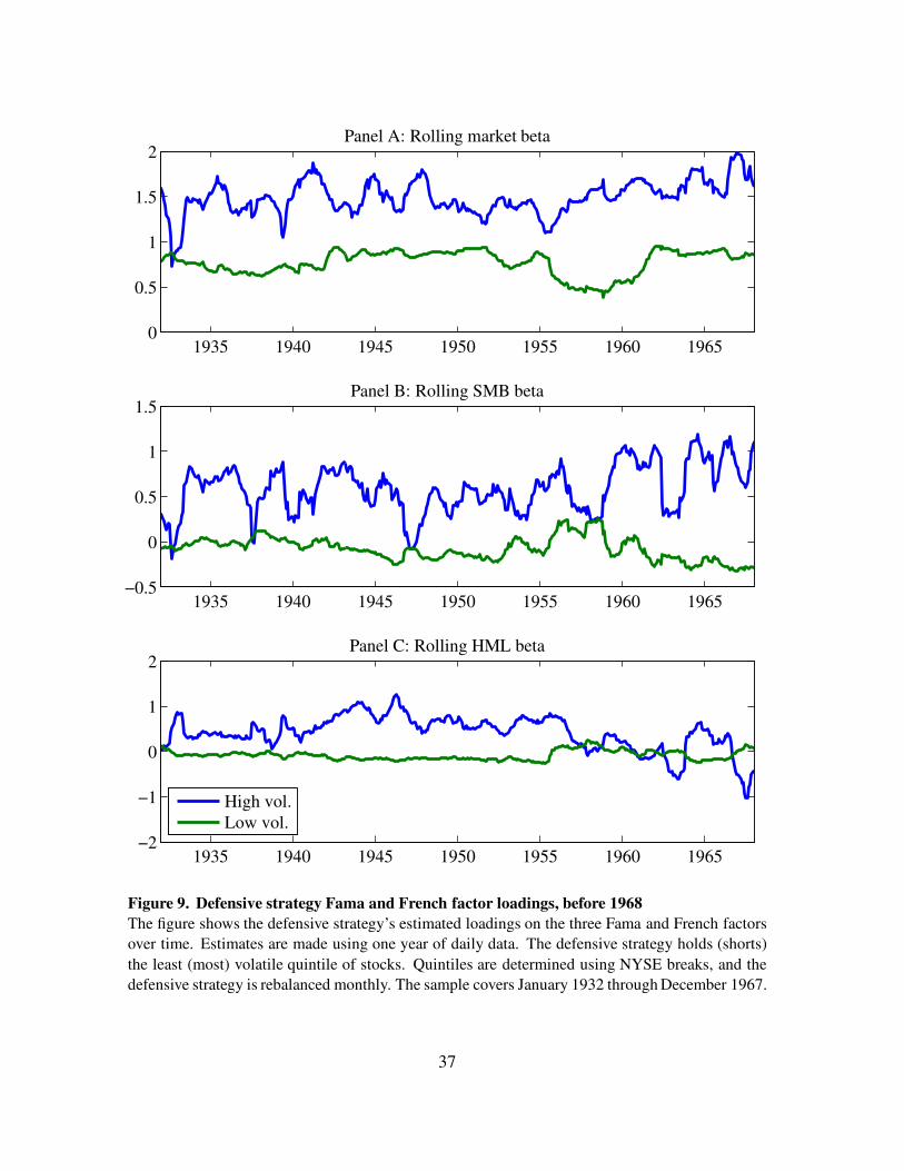
factor loadings. In fact, for much of the pre-1968 sample defensive strategies tilted strongly

to growth, not value, which helps explain why defensive stocks have only provided higher

returns than aggressive stocks in the post-1967 sample (for pre-1968 defensive strategy factor

loadings see Figure 9, in the Appendix). The extreme defensive strategy growth tilt observed

around 2010 is mostly due to a sharp concurrent widening of the volatility spread between the

most and least profitable stocks. At this time the high volatility portfolio became increasingly

dominated by less profitable stocks, which on average have lower valuations. The defensive

strategy’s peak HML loading is cut 55% by accounting for its large negative profitability

tilt (i.e., in four-factor rolling regressions, which additionally include a profitable-minus-

unprofitable factor, constructed in the same manner as HML on the basis of operating profits-

to-assets instead of book-to-market).

24

1970 1975 1980 1985 1990 1995 2000 2005 20100.5

1

1.5

2Panel A: Rolling market beta

1970 1975 1980 1985 1990 1995 2000 2005 2010−0.5

0

0.5

1

1.5Panel B: Rolling SMB beta

1970 1975 1980 1985 1990 1995 2000 2005 2010−2

−1

0

1

2

High vol.

Low vol.

Panel C: Rolling HML beta

Figure 6. Defensive strategy Fama and French factor loadings

The figure shows the defensive strategy’s estimated loadings on the three Fama and French factors

over time. Estimates are made using one year of daily data. The defensive strategy holds (shorts)

the least (most) volatile quintile of stocks. Quintiles are determined using NYSE breaks, and the

defensive strategy is rebalanced monthly. The sample covers January 1968 through December 2013.

25

Value of $1 invested in 1968 in hedged volatility strategies

1970 1975 1980 1985 1990 1995 2000 2005 2010

$1

$10

Low volatility234High volatilityT−Bills

Unprofitable small growth

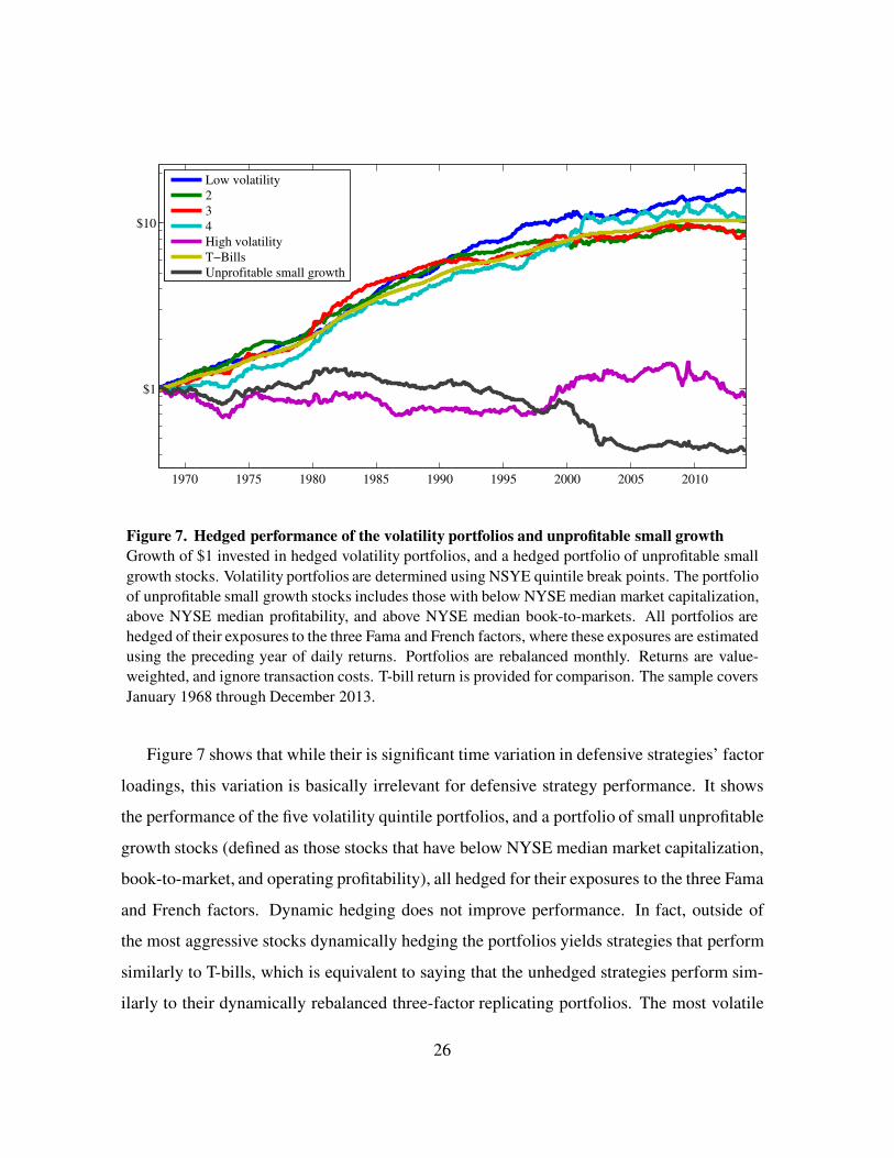
Figure 7. Hedged performance of the volatility portfolios and unprofitable small growth

Growth of $1 invested in hedged volatility portfolios, and a hedged portfolio of unprofitable small

growth stocks. Volatility portfolios are determined using NSYE quintile break points. The portfolio

of unprofitable small growth stocks includes those with below NYSE median market capitalization,

above NYSE median profitability, and above NYSE median book-to-markets. All portfolios are

hedged of their exposures to the three Fama and French factors, where these exposures are estimated

using the preceding year of daily returns. Portfolios are rebalanced monthly. Returns are value-

weighted, and ignore transaction costs. T-bill return is provided for comparison. The sample covers


Figure 7 shows that while their is significant time variation in defensive strategies’ factor

loadings, this variation is basically irrelevant for defensive strategy performance. It shows

the performance of the five volatility quintile portfolios, and a portfolio of small unprofitable

growth stocks (defined as those stocks that have below NYSE median market capitalization,

book-to-market, and operating profitability), all hedged for their exposures to the three Fama

and French factors. Dynamic hedging does not improve performance. In fact, outside of

the most aggressive stocks dynamically hedging the portfolios yields strategies that perform

similarly to T-bills, which is equivalent to saying that the unhedged strategies perform sim-

ilarly to their dynamically rebalanced three-factor replicating portfolios. The most volatile

26

stocks, hedged of their exposure to the three Fama and French factors, significantly under-

perform T-bills, but do not perform as poorly as the hedged portfolio of small unprofitable

growth stocks that they most closely resemble.

6 Conclusion

Over the last 45 years defensive stocks have delivered higher returns than the most aggressive

stocks, and defensive strategies, at least those based on volatility, have delivered significant

Fama and French three-factor alphas. This performance is not at all anomalous, however, af-

ter properly controlling for size, relative valuations, and, most critically, profitability. While

investors would have benefited from a defensive tilt over the period, these benefits derive ef-

fectively from an unprofitable small growth exclusion, which could have been implemented

more efficiently, and at lower cost, directly.

27

A Additional results

Value of $1 invested in 1931 in volatility portfolios (log scale)

1935 1940 1945 1950 1955 1960 1965

$1

$10

Low vol.

2

3

4

High vol.

Value of $1 invested in 1931 in beta portfolios (log scale)

1935 1940 1945 1950 1955 1960 1965

$1

$10

$100

Low beta

2

3

4

High beta

Figure 8. Pre-1968 performance of volatility and beta quintiles

Growth of $1 invested in quintile portfolios sorted on volatility (top panel) and beta (bottom panel).

Volatilities and beta are estimated using one year of daily data when available, and five years of

monthly data otherwise. Portfolios are rebalanced monthly and ignore transaction costs, and returns

are value-weighted. The sample covers January 1931 through December 1967.

28

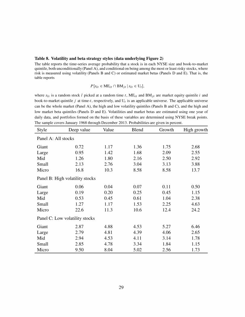
Table 8. Volatility and beta strategy styles (data underlying Figure 2)

The table reports the time-series average probability that a stock is in each NYSE size and book-to-marketquintile, both unconditionally (Panel A), and conditional on being among the most or least risky stocks, whererisk is measured using volatility (Panels B and C) or estimated market betas (Panels D and E). That is, thetable reports

P Œslt 2 MEi t \ BMjt j slt 2 Ut �;

where slt is a random stock l picked at a random time t , MEi t and BMjt are market equity quintile i and

book-to-market quintile j at time-t , respectively, and Ut is an applicable universe. The applicable universe

can be the whole market (Panel A), the high and low volatility quintiles (Panels B and C), and the high and

low market beta quintiles (Panels D and E). Volatilities and market betas are estimated using one year of

daily data, and portfolios formed on the basis of these variables are determined using NYSE break points.

The sample covers January 1968 through December 2013. Probabilities are given in percent.

Style Deep value Value Blend Growth High growth

Panel A: All stocks

Giant 0.72 1.17 1.36 1.75 2.68

Large 0.95 1.42 1.68 2.09 2.55

Mid 1.26 1.80 2.16 2.50 2.92

Small 2.13 2.76 3.04 3.13 3.88

Micro 16.8 10.3 8.58 8.58 13.7

Panel B: High volatility stocks

Giant 0.06 0.04 0.07 0.11 0.50

Large 0.19 0.20 0.25 0.45 1.15

Mid 0.53 0.45 0.61 1.04 2.38

Small 1.27 1.17 1.53 2.25 4.63

Micro 22.6 11.3 10.6 12.4 24.2

Panel C: Low volatility stocks

Giant 2.87 4.88 4.53 5.27 6.46

Large 2.79 4.81 4.39 4.06 2.65

Mid 2.94 4.53 4.11 3.14 1.78

Small 2.85 4.78 3.34 1.84 1.15

Micro 9.50 8.04 5.02 2.56 1.73

29

Table 8 (continued)

Style Deep value Value Blend Growth High growth

Panel D: High beta stocks

Giant 0.48 0.73 1.01 1.69 3.27

Large 0.89 1.07 1.52 2.22 4.25

Mid 1.32 1.38 2.03 3.00 5.61

Small 2.31 2.31 2.99 4.44 7.52

Micro 9.83 6.28 7.07 9.09 17.7

Panel E: Low beta stocks

Giant 0.62 1.23 0.99 0.97 1.30

Large 0.75 1.50 1.41 1.16 1.02

Mid 1.12 1.89 1.77 1.41 1.06

Small 1.70 2.79 2.39 1.75 1.43

Micro 26.3 15.1 10.5 8.3 11.7

Table 9. Market beta correlates

The table reports Fama and MacBeth (1973) regressions of volatility onto variables known to predict cross-

sectional variation in returns. Because of the persistence in the variables Newey and West t-statistics are

reported, calculated using 60 monthly lags. The sample covers January 1968 through December 2013.

Predictor variable (1) (2) (3) (4) (5)

Size (ln(ME)) 0.07 0.14[4.82] [15.7]

Value (ln(B/M)) -0.17 -0.06[-8.96] [-4.34]

Profitability�

GP�SGAA

�

0.07 0.20[0.63] [3.26]

Leverage (B/A) 0.54 1.02[3.07] [5.49]

Mean-R2 (%) 8.6 6.2 1.0 8.1 26.7

30

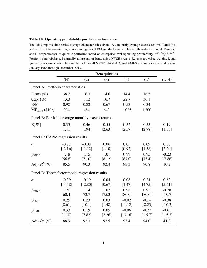
Table 10. Operating profitability portfolio performance

The table reports time-series average characteristics (Panel A), monthly average excess returns (Panel B),

and results of time-series regressions using the CAPM and the Fama and French three-factor model (Panels C

and D, respectively), of quintile portfolios sorted on enterprise level operating profitability, REV�COGS�SGAA

.

Portfolios are rebalanced annually, at hte end of June, using NYSE breaks. Returns are value-weighted, and

ignore transaction costs. The sample includes all NYSE, NASDAQ, and AMEX common stocks, and covers


Beta quintiles

(H) (2) (3) (4) (L) (L-H)


Firms (%) 38.2 16.3 14.6 14.4 16.5

Cap. (%) 13.3 11.2 16.7 22.7 36.1

B/M 0.90 0.82 0.67 0.53 0.34

ME2013 ($106) 204 484 643 1,025 1,200


E[Re] 0.35 0.46 0.55 0.52 0.55 0.19[1.41] [1.94] [2.63] [2.57] [2.78] [1.33]


˛ -0.21 -0.08 0.06 0.05 0.09 0.30[-2.16] [-1.12] [1.10] [0.92] [1.58] [2.20]

ˇMKT 1.18 1.15 1.01 0.99 0.95 -0.23[56.6] [71.0] [81.2] [87.0] [73.4] [-7.86]

Adj.-R2 (%) 85.5 90.3 92.4 93.3 90.8 10.2


˛ -0.39 -0.19 0.04 0.08 0.24 0.62[-4.48] [-2.80] [0.67] [1.47] [4.75] [5.51]

ˇMKT 1.20 1.14 1.02 0.98 0.92 -0.28[60.4] [72.7] [75.3] [80.0] [80.6] [-10.7]

ˇSMB 0.25 0.23 0.03 -0.02 -0.14 -0.38[8.61] [10.1] [1.48] [-1.12] [-8.23] [-10.2]

ˇHML 0.33 0.19 0.05 -0.06 -0.27 -0.61[11.0] [7.82] [2.26] [-3.16] [-15.7] [-15.3]

Adj.-R2 (%) 88.9 92.3 92.5 93.4 94.0 41.8

31

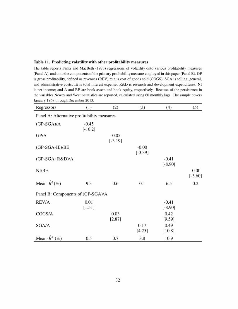
Table 11. Predicting volatility with other profitability measures

The table reports Fama and MacBeth (1973) regressions of volatility onto various profitability measures

(Panel A), and onto the components of the primary profitability measure employed in this paper (Panel B). GP

is gross profitability, defined as revenues (REV) minus cost of goods sold (COGS); SGA is selling, general,

and administrative costs; IE is total interest expense; R&D is research and development expenditures; NI

is net income; and A and BE are book assets and book equity, respectively. Because of the persistence in

the variables Newey and West t-statistics are reported, calculated using 60 monthly lags. The sample covers


Regressors (1) (2) (3) (4) (5)

Panel A: Alternative profitability measures

(GP-SGA)/A -0.45[-10.2]

GP/A -0.05[-3.19]

(GP-SGA-IE)/BE -0.00[-3.39]

(GP-SGA+R&D)/A -0.41[-8.90]

NI/BE -0.00[-3.60]

Mean- OR2.%/ 9.3 0.6 0.1 6.5 0.2

Panel B: Components of (GP-SGA)/A

REV/A 0.01 -0.41[1.51] [-8.90]

COGS/A 0.03 0.42[2.87] [9.59]

SGA/A 0.17 0.49[4.25] [10.8]

Mean- OR2 (%) 0.5 0.7 3.8 10.9

32

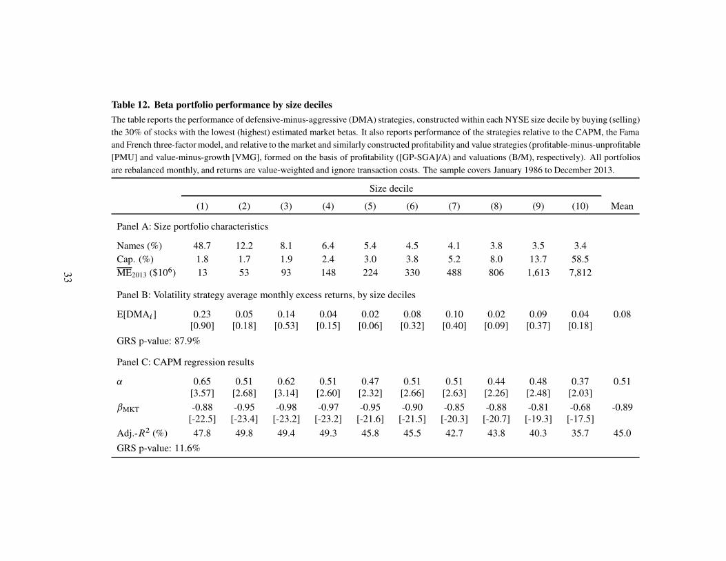
Table 12. Beta portfolio performance by size deciles

The table reports the performance of defensive-minus-aggressive (DMA) strategies, constructed within each NYSE size decile by buying (selling)

the 30% of stocks with the lowest (highest) estimated market betas. It also reports performance of the strategies relative to the CAPM, the Fama

and French three-factor model, and relative to the market and similarly constructed profitability and value strategies (profitable-minus-unprofitable

[PMU] and value-minus-growth [VMG], formed on the basis of profitability ([GP-SGA]/A) and valuations (B/M), respectively). All portfolios

are rebalanced monthly, and returns are value-weighted and ignore transaction costs. The sample covers January 1986 to December 2013.

Size decile

(1) (2) (3) (4) (5) (6) (7) (8) (9) (10) Mean

Panel A: Size portfolio characteristics

Names (%) 48.7 12.2 8.1 6.4 5.4 4.5 4.1 3.8 3.5 3.4

Cap. (%) 1.8 1.7 1.9 2.4 3.0 3.8 5.2 8.0 13.7 58.5

ME2013 ($106) 13 53 93 148 224 330 488 806 1,613 7,812

Panel B: Volatility strategy average monthly excess returns, by size deciles

E[DMAi ] 0.23 0.05 0.14 0.04 0.02 0.08 0.10 0.02 0.09 0.04 0.08[0.90] [0.18] [0.53] [0.15] [0.06] [0.32] [0.40] [0.09] [0.37] [0.18]

GRS p-value: 87.9%


˛ 0.65 0.51 0.62 0.51 0.47 0.51 0.51 0.44 0.48 0.37 0.51[3.57] [2.68] [3.14] [2.60] [2.32] [2.66] [2.63] [2.26] [2.48] [2.03]

ˇMKT -0.88 -0.95 -0.98 -0.97 -0.95 -0.90 -0.85 -0.88 -0.81 -0.68 -0.89[-22.5] [-23.4] [-23.2] [-23.2] [-21.6] [-21.5] [-20.3] [-20.7] [-19.3] [-17.5]

Adj.-R2 (%) 47.8 49.8 49.4 49.3 45.8 45.5 42.7 43.8 40.3 35.7 45.0

GRS p-value: 11.6%

33

Table 12 (continued)

Size decile

(1) (2) (3) (4) (5) (6) (7) (8) (9) (10) Mean

Panel D: Fama and French three-factor model regression results: DMAi D ˛ C ˇMKTMKT C ˇSMBSMB C ˇHMLHML

˛ 0.63 0.39 0.40 0.27 0.17 0.22 0.20 0.11 0.17 0.09 0.26[3.83] [2.43] [2.48] [1.72] [1.04] [1.44] [1.31] [0.68] [1.02] [0.57]

ˇMKT -0.72 -0.74 -0.74 -0.72 -0.66 -0.63 -0.59 -0.63 -0.57 -0.52 -0.65[-19.0] [-19.9] [-19.5] [-19.6] [-18.1] [-18.0] [-16.4] [-16.9] [-15.2] [-13.7]

ˇSMB -0.63 -0.69 -0.64 -0.64 -0.64 -0.60 -0.55 -0.45 -0.43 -0.19 -0.55[-11.7] [-13.0] [-11.8] [-12.2] [-12.2] [-12.0] [-10.7] [-8.51] [-7.95] [-3.39]

ˇHML 0.17 0.37 0.55 0.60 0.75 0.72 0.73 0.77 0.73 0.59 0.60[2.92] [6.47] [9.55] [10.7] [13.4] [13.6] [13.4] [13.6] [12.6] [10.2]

Adj.-R2 (%) 59.5 65.0 66.0 67.5 68.1 68.0 64.8 63.5 59.4 47.8 62.9

GRS p-value: 6.0%

Panel E: Conditional three-factor regression results: DMAi D ˛ C ˇMKTMKT C ˇPMUiPMUi C ˇVMGi

VMGi

˛ -0.24 -0.28 -0.03 -0.10 -0.15 -0.05 -0.11 0.03 0.02 0.19 -0.07[-1.67] [-1.82] [-0.19] [-0.65] [-0.98] [-0.32] [-0.75] [0.23] [0.13] [1.08]

ˇMKT -0.65 -0.70 -0.69 -0.70 -0.64 -0.58 -0.54 -0.54 -0.47 -0.55 -0.61[-20.2] [-20.1] [-19.2] [-19.3] [-18.1] [-16.5] [-16.2] [-15.5] [-14.4] [-13.4]

ˇPMUi0.34 0.27 0.36 0.29 0.30 0.35 0.46 0.49 0.51 0.39 0.38

[8.15] [5.85] [7.58] [6.26] [6.68] [7.66] [9.36] [10.2] [10.9] [5.04]

ˇVMGi0.47 0.61 0.63 0.74 0.78 0.80 0.89 0.87 0.88 0.57 0.72

[10.1] [16.0] [17.0] [17.7] [20.2] [19.6] [22.5] [21.9] [23.2] [8.46]

Adj.-R2 (%) 70.2 69.6 69.9 68.8 70.6 68.4 70.6 70.5 70.7 43.1 39.3


34

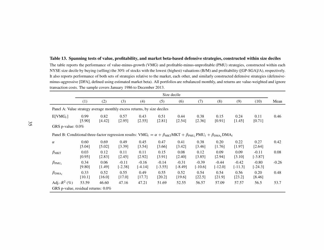
Table 13. Spanning tests of value, profitability, and market beta-based defensive strategies, constructed within size deciles

The table reports the performance of value-minus-growth (VMG) and profitable-minus-unprofitable (PMU) strategies, constructed within each

NYSE size decile by buying (selling) the 30% of stocks with the lowest (highest) valuations (B/M) and profitability ([GP-SGA]/A), respectively.

It also reports performance of both sets of strategies relative to the market, each other, and similarly constructed defensive strategies (defensive-

minus-aggressive [DFA], defined using estimated market beta). All portfolios are rebalanced monthly, and returns are value-weighted and ignore

transaction costs. The sample covers January 1986 to December 2013.

Size decile

(1) (2) (3) (4) (5) (6) (7) (8) (9) (10) Mean

Panel A: Value strategy average monthly excess returns, by size deciles

E[VMGi ] 0.99 0.82 0.57 0.43 0.51 0.44 0.38 0.15 0.24 0.11 0.46[5.90] [4.42] [2.95] [2.55] [2.81] [2.54] [2.36] [0.91] [1.45] [0.71]

GRS p-value: 0.0%

Panel B: Conditional three-factor regression results: VMGi D ˛ C ˇMKTMKT C ˇPMUiPMUi C ˇDMAi

DMAi

˛ 0.60 0.69 0.49 0.45 0.47 0.41 0.38 0.20 0.22 0.27 0.42[5.04] [5.02] [3.39] [3.54] [3.66] [3.42] [3.46] [1.76] [1.97] [2.64]

ˇMKT 0.03 0.12 0.11 0.11 0.15 0.08 0.12 0.09 0.09 -0.11 0.08[0.95] [2.83] [2.45] [2.92] [3.91] [2.40] [3.85] [2.94] [3.10] [-3.87]

ˇPMUi0.34 0.06 -0.11 -0.16 -0.14 -0.31 -0.39 -0.44 -0.42 -0.80 -0.26

[9.80] [1.49] [-2.38] [-4.14] [-3.55] [-8.49] [-10.6] [-12.0] [-11.3] [-24.3]

ˇDMAi0.33 0.52 0.55 0.49 0.55 0.52 0.54 0.54 0.56 0.20 0.48

[10.1] [16.0] [17.0] [17.7] [20.2] [19.6] [22.5] [21.9] [23.2] [8.46]

Adj.-R2 (%) 53.59 46.60 47.16 47.21 51.69 52.55 56.57 57.09 57.57 56.5 53.7


35

Table 13 (continued)

Size decile

(1) (2) (3) (4) (5) (6) (7) (8) (9) (10) Mean

Panel C: Profitability strategy average monthly excess returns, by size deciles

E[PMUi ] 0.90 0.60 0.42 0.54 0.27 0.19 0.27 0.23 0.18 0.15 0.37[5.07] [4.26] [3.06] [3.85] [1.89] [1.34] [2.12] [1.72] [1.36] [1.10]

GRS p-value: 0.0%

Panel D: Conditional three-factor regression results: PMUi D ˛ C ˇMKTMKT C ˇPMUiVMGi C ˇDMAi

DMAi

˛ 0.29 0.47 0.35 0.55 0.30 0.31 0.40 0.30 0.25 0.29 0.35[2.10] [3.40] [2.66] [3.95] [2.11] [2.38] [3.47] [2.53] [2.21] [3.14]

ˇMKT 0.21 0.15 0.17 0.14 0.11 0.03 0.01 -0.00 0.00 -0.16 0.07[5.23] [3.75] [4.28] [3.38] [2.66] [0.70] [0.36] [-0.02] [0.04] [-6.34]

ˇDMAi0.31 0.22 0.26 0.23 0.25 0.27 0.30 0.33 0.35 0.11 0.26

[8.15] [5.85] [7.58] [6.26] [6.68] [7.66] [9.36] [10.2] [10.9] [5.04]

ˇVMGi0.44 0.06 -0.09 -0.19 -0.16 -0.37 -0.43 -0.47 -0.45 -0.65 -0.23

[9.80] [1.49] [-2.38] [-4.14] [-3.55] [-8.49] [-10.6] [-12.0] [-11.3] [-24.3]

Adj.-R2 (%) 45.50 12.38 10.45 6.27 8.03 13.91 20.77 25.05 25.01 54.2 22.2


36

1935 1940 1945 1950 1955 1960 19650

0.5

1

1.5

2Panel A: Rolling market beta

1935 1940 1945 1950 1955 1960 1965−0.5

0

0.5

1

1.5Panel B: Rolling SMB beta

1935 1940 1945 1950 1955 1960 1965−2

−1

0

1

2

High vol.

Low vol.

Panel C: Rolling HML beta

Figure 9. Defensive strategy Fama and French factor loadings, before 1968

The figure shows the defensive strategy’s estimated loadings on the three Fama and French factors

over time. Estimates are made using one year of daily data. The defensive strategy holds (shorts)

the least (most) volatile quintile of stocks. Quintiles are determined using NYSE breaks, and the

defensive strategy is rebalanced monthly. The sample covers January 1932 through December 1967.

37

References

[1] Ang, A., Hodrick, R., Xing, Y., Zhang, X., 2006. The cross-section of volatility and expected

returns. Journal of Finance 61, 259–299.

[2] Asness, C., Frazzini, A., Pedersen, L.H., 2014. Low-risk investing without industry bets. Finan-

cial Analysts Journal 70, 24–41.

[3] Ball, R., Gerakos, J., Linnainmaa, j., Nikolaev, V., 2014. Deflating profitability. University of

Chicago working paper.

[4] Baker, M., Bradley, B., Wurgler, J., 2011. Benchmarks as limits to arbitrage: understanding the

low-volatility anomaly. Financial Analysts Journal 67, 1–15.

[5] Bali, T.G., Caici, N., 2008. Idiosyncratic volatility and the cross section of expected returns.

Journal of Financial and Quantitative Analysis 43, 29–58.

[6] Blitz, D., Van Vliet, P., 2007. The volatility effect: Lower risk without lower return. Journal of

Portfolio Management, 102–113.

[7] Black, F., 1972. Capital market equilibrium with restricted borrowing. Journal of Business 45,

444–455.

[8] Black, F., Jensen, M. C., Scholes, M., 1972. The Capital Asset Pricing Model: Some empirical

tests. In Studies in the Theory of Capital Markets (Jensen, M.C. editor). Praeger, New York.

[9] Fama, E.F., French, K.R., 1993. Common risk factors in the returns on stocks and bonds. Journal

of Financial Economics 33, 3–56.

[10] Fama, E.F., French, K.R., 2014. A five-factor asset pricing model. University of Chicago work-

ing paper.

[11] Fama, E. F., MacBeth, J. D., 1973. Risk, return, and equilibrium: empirical tests. Journal of

Political Economy 81, 607–636.

[12] Frazzini, A., Pedersen, L.H., 2014. Betting against beta. Journal of Financial Economics 111,

1–25.

[13] Gibbons, M.R., Ross, S.A., Shanken, J., 1989. A test of the efficiency of a given portfolio.

Econometrics 57, 1121–1152.

[14] Li X., Sullivan, R.N., Garcia-Feijoo, L., 2014. The limits to arbitrage and the low-volatility

anomaly. Financial Analysts Journal 70, 52–63.

[15] Newey, W.K., West, K.D., 1987. A simple, positive semi-definite, heteroskedasticity and auto-

correlation consistent covariance matrix. Econometrica 55, 703–708.

[16] Novy-Marx, R., 2013. The other side of value: The gross profitability premium. Journal of

Financial Economics 108, 1–28.

38

Documents

NBER WORKING PAPER SERIES UNDERSTANDING … · Robert Novy-Marx Working Paper 20591 ... Section 6 concludes. ... and small cap and value tilts to the low beta portfolios, though these