Embed Size (px)
Citation preview
NBER WORKING PAPER SERIES
HOW DO MONETARY AND FISCAL POLICYINTERACT IN THE EUROPEAN MONETARY UNION?
Matthew B. CanzoneriRobert CumbyBehzad Diba
Working Paper 11055http://www.nber.org/papers/w11055
NATIONAL BUREAU OF ECONOMIC RESEARCH1050 Massachusetts Avenue
Cambridge, MA 02138January 2005
Prepared for the NBER’s ISOM in Reykjavik, Iceland, June 18-19, 2004.The views expressed herein arethose of the author(s) and do not necessarily reflect the views of the National Bureau of Economic Research.
© 2005 by Matthew B. Canzoneri, Robert Cumby, and Behzad Diba. All rights reserved. Short sections oftext, not to exceed two paragraphs, may be quoted without explicit permission provided that full credit,including © notice, is given to the source.
How Do Monetary and Fiscal Policy Interact in the European Monetary Union?Matthew B. Canzoneri, Robert Cumby, and Behzad DibaNBER Working Paper No. 11055January 2005JEL No. E63, F33
ABSTRACT
Formation of the Euro area raises new questions about the coordination of monetary and fiscal
policy. Using a New Neoclassical Synthesis (NNS) model, we show that a common monetary policy,
responding to area-wide aggregates, has asymmetric effects on countries within the union, depending
on whether they are large or small, or whether they have high or low debts. We analyze the
implications of these asymmetries for the various countries welfare and for their fiscal policies. We
also study rules for setting national tax and spending rates, rules that constrain movements in the
deficit to GDP ratio. We ask whether these rules are necessary for the common monetary policy to
be able to harmonize national inflation rates, and we analyze their effects on national welfare. We
also discuss some potential failings of our model (and perhaps NNS models generally); in particular,
our model’s variance decompositions suggest that productivity shocks may play an inordinately large
role, while fiscal shocks (or demand shocks generally) may play too small a role (even when ‘rule
of thumb’ spenders are added).
Matthew B. CanzoneriDepartment of EconomicsGeorgetown UniversityWashington, DC [email protected]
Robert E. CumbyDepartment of EconomicsGeorgetown UniversityWashington, DC 20057and [email protected]
Behzad T. DibaDepartment of EconomicsGeorgetown UniversityWashington, DC [email protected]
1 Goodfriend and King (1997) outlined the New Neoclassical Synthesis, and gave it thename. Woodford (2003) provides a masterful introduction to this class of models.
2 See Clarida, Gali and Gertler (1999) and Canzoneri, Cumby and Diba (2003).
1. Introduction
Formation of the Euro area raises new questions about the coordination of monetary and
fiscal policy. Twelve countries – each with its own tax and spending policies – are now married by
a common monetary policy. Does the common monetary policy have the same effect in each of the
countries, and the same implications for fiscal policy? Or, does it affect high debt countries in a
different way than low debt countries? Does it favor big countries over small countries? And, how
does the existence of twelve separate fiscal policies affect the European Central Bank’s (ECB)
ability to control inflation? In particular, is the lack of coordination of national fiscal policies a
major source of the rather surprising diversity of national inflation rates we have observed since the
Euro’s inception? And, is the consequent diversity of national real interest rates a source of
macroeconomic instability? If so, does this point to a need for constraints on deficits, as embodied
in the Stability and Growth Pact (SGP)? Or, does the SGP itself create a new source of instability
at the national level?
In this paper, we try to address these questions within the context of the New Neoclassical
Synthesis (NNS).1 The NNS is characterized by optimizing agents and some form of nominal inertia.
Thus, the NNS provides a natural framework to study the interactions between monetary and fiscal
policy: its neoclassical underpinnings allow us to analyze the positive and normative implications
of distortionary taxation, while its assumption of nominal inertia allows us to assess the implications
of these microeconomic aspects of fiscal policy for macroeconomic stability.
The NNS has been used extensively to analyze monetary policy.2 Integrating fiscal policy

-2-
3 Examples include Benigno and Woodford (2003), Kollmann (2003), and Uribe andSchmitt-Grohe (2003, 2004).
4 Duarte and Wolman (2002) is a notable example; we will discuss their work below.
has however been slow. There have been papers analyzing the theory of optimal monetary and fiscal
policy,3 but quantitative analyses are scarce.4 There is, of course, a reason for this. It has been
difficult to make NNS models replicate stylized facts about fiscal policy, facts that are taken from
the recent empirical literature. We will discuss some potential problems with our current modeling
effort, and it should be admitted at the outset that these problems may be driving some of our results.
In this sense, we view our paper as the beginning of a research agenda, and not as the final word on
policy coordination within a monetary union.
We do not attempt a serious calibration to any particular country; instead, we calibrate a
series of models that seem to capture important aspects of the interaction between monetary and
fiscal policy in the Euro area. An empirical investigation of the relationship between the aggregate
Euro area inflation rate and national inflation rates, and various aspects of fiscal policy within the
Euro area, suggests that we calibrate our model to an “Average” (small) Country, a High Debt
Country, and a Large Country. Then, we ask how the common monetary policy impinges on
national fiscal policy and national welfare in each of these ‘countries’, and how uncoordinated
national fiscal policies impinge on the ECB’s ability to control inflation. We show that the common
monetary policy has asymmetric effects on the three countries: the effects differ between the
Average Country and the High Debt Country (not too surprisingly) because the latter’s fiscal
position is more sensitivity to changes in debt payments, and the effects differ between the Average
Country and the Large Country (perhaps more surprisingly) because the latter’s inflation rate is more
-3-
highly correlated with aggregate Euro area inflation.
It may be best to summarize our basic results for the coordination of monetary and fiscal
policy at the outset:
! Productivity shocks and idiosyncratic monetary policy shocks explain 70% of the volatility
in the deficit-to-GDP ratio in our Average and Large Countries, and 80% in our High Debt
Country. Rules (like the SGP) that try to discipline fiscal policy by requiring governments
to limit the unconditional standard deviation of the debt-to-GDP ratio seem rather perverse
in this context.
! Productivity shocks are the dominant source of inflation differentials in all versions of our
model, followed by idiosyncratic monetary policy shocks. Shocks to tax rates and spending
play a minor role. These results are not changed by the inclusion of ‘rule of thumb’
consumers (which augments the effect of fiscal shocks on aggregate demand). The large
inflation differentials observed in the Euro area do not, according to our models, point to the
need for coordination of national fiscal policies.
! Our model suggests that if constraints on deficits are deemed necessary in the Euro area,
then there are advantages to doing so by requiring that government purchases, rather than
the wage tax rate, respond to the deficit. In fact, our model suggests that such a constraint
may actually be welfare enhancing, since government spending crowds out private
consumption in our model. But as we discuss below, this result may be driven by
problematic features of our model.
! Deficits are more sensitive to interest rates in high debt countries, due to the burden of debt
service. In addition, high debt countries tend to have higher tax rates, increasing tax

-4-
distortions, and making tax revenues more sensitive to changes in the tax base. Not
surprisingly, these factors lead to welfare costs: the typical household in our High Debt
Country would be willing give up 1.3% percent of its consumption each period to live in the
Average Country.
! Our model suggests that the common monetary policy favors larger countries in the Euro
area, since their inflation rates are more highly correlated with aggregate (Euro area)
inflation. For example, the welfare cost of business cycles in our Average Country is four
times larger than in our Large Country.
As noted earlier, some of these results may be driven by potential weaknesses in our NNS
modeling. In particular, the role played by productivity shocks appears to be excessive in our
models. And, an increase in government purchases crowds out private consumption; this is
inconsistent with empirical work by Fatas and Mihov (2000, 2001), Blanchard and Perotti (2002)
and Canzoneri, Cumby and Diba (2002). In an attempt to address the consumption paradox, and to
enhance the role of demand side shocks, we add ‘rule of thumb’ consumers in the last section of the
paper. However, this experiment in NNS modeling does not change any of our basic conclusions.
The rest of the paper is organized as follows: In Section 2, we outline our basic NNS frame-
work and explain how we calculate national welfare; then, we present an empirical analysis that
documents various aspects of fiscal policy in the Euro area and how movements in national inflation
rates affect the aggregate Euro area inflation rate; and finally, on the basis of this empirical analysis,
we calibrate our model for an Average Country, a High Debt Country and a Large Country. In
Section 3, we provide an overview of the performance of each version of the model, focusing
especially on the role of productivity shocks. In Section 4, we explain why the common monetary

-5-
policy has asymmetric affects across the Euro area, and we discuss the ways in which it impinges
upon national fiscal policy and welfare. Some people believe that constraints on the size of deficits
are necessary in a monetary union; so, in Section 5, we discuss rules for the wage tax or government
spending which limit fluctuations in the deficit to GDP ratio; we assess their positive and normative
effects. In Section 6, we discuss the ways in which fiscal policy impinges on the ECB’s ability to
control inflation across the Euro area, and the possible need for fiscal constraint to control inflation
differentials across the Euro area; we also discuss some anomalies in the way changes government
purchases affect private consumption and investment. In Section 7, we introduce ‘rule of thumb’
agents to try to address some of those anomalies. And in Section 8, we conclude with a discussion
of future research.
2. A Model of Euro Area Economies
We begin in Section 2.A with a description of the basic theoretical framework. In Section
2.B, we provide an empirical analysis of national inflation differentials, and of national tax and
spending policies. We draw on this empirical work to calibrate a benchmark model to our three
typical country profiles: a typical small country, a typical high debt country, and a typical large
country. In the remainder of the paper, we use the model to discuss the interaction between
monetary and fiscal policy in the Euro area.
2. A. The Theoretical Framework
Like other NNS models, our model is characterized by optimizing agents, monopolistic
competition, and nominal inertia. Our basic framework is most closely related to those in Erceg,
Henderson and Levin (2000) and Collard and Dellas (2003): as in Collard and Dellas (2003), we
allow for capital accumulation, and we calculate second order approximations to both the model and

-6-
5 Although the aggregate capital stock will be predetermined in our model, we areassuming that capital is mobile across firms. Thus, in our notation, Kt-1(f) stands for firm f’schoice of its capital input at time t.
the welfare function; as in Erceg, Henderson and Levin (2000), we allow for both wage and price
inertia. Our framework differs from theirs in that we introduce distortionary taxation (on
consumption and labor income) and debt dynamics.
2.A.1. Firms’ price setting behavior –
There is a continuum of firms – indexed by f – on the unit interval. At time t, each firm rents
capital Kt-1(f) at the rate Rt, hires a labor bundle Nt(f) at the rate Wt, and produces a differentiated
product5
(1) Yt(f) = ZtKt-1(f)<Nt(f)<-1,
where 0 < < < 1, and Zt is an economy wide productivity shock that follows an autoregressive
process – log(Zt) = Dlog(Zt-1) + ,p,t. The firm’s cost minimization problem implies
(2) Rt/Wt = [</(1-<)](Nt(f)/Kt-1(f)),
and the firm’s marginal cost can be expressed as
(3) MCt(f) = [<<(1-<)(1-<)]-1Rt<Wt
1-</Zt.
A composite good
(4) Yt = [I10Yt(f)(Np-1)/Npdf]Np/(Np-1), Np > 1,
can be used as either a consumption good or capital. The good’s price, which can be interpreted as
the aggregate price level, is given by
(5) Pt = [I10Pt(f)1-Npdf]1/(1-Np),
and demand for the product of firm f is given by
(6) Ydt(f) = (Pt /Pt(f))NpYt.

-7-
Following Calvo (1983), firms set prices in staggered ‘contracts’ of random duration. In any
period t, each firm gets to announce a new price with probability (1-"); otherwise, the old contract,
and its price, remains in effect. If firm f gets to announce a new contract in period t, it chooses a
new price Pt*(f) to maximize the value of its profit stream over states of nature in which the new price
is expected to hold:
(7) Et3 j4
=t("$)j-t8j[Pt*(f)Yj(f) - TCj(f)],
where TC(f) is the firm’s total cost, $ is the households’ discount factor, and 8j is the households’
marginal utility of nominal wealth (to be defined below). The firm’s first order condition is
(8) Pt* = :p(PBt/PAt),
where :p = Np/(Np - 1) is a monopoly markup factor, and
(9) PBt = Et3 j4
=t("$)j-t8jMCj(f)PjNpYj = "$EtPBt+1 + 8tMCt(f)Pt
NpYt
(10) PAt = Et3 j4
=t("$)j-t8jPjNpYj = "$EtPAt+1 + 8tPt
NpYt
As " 6 0, all firms reset their prices each period (the flexible price case), and Pt*(f) 6 :pMCt(f).
Since the markup is positive (:p > 1), output will be inefficiently low in the flexible price solution.
2.A.2. Households’ wage setting behavior and capital accumulation –
There is a continuum of households indexed by h on the unit interval. Each household
supplies a differentiated labor service to all of the firms in the economy. The composite labor
bundle
(11) Nt = [I10Lt(h)(Nw-1)/Nwdh]Nw/(Nw-1), Nw > 1,
reflects the firms’ production technology. Cost minimization implies that the bundle’s wage is
(12) Wt = [I10Wt(h)1-Nwdh]1/(1-Nw),
and demand for the labor of household h is
-8-
6 The utility function (and budget constraint below) should also include a term in realmoney balances, but we follow much of the NNS literature in assuming that this term isnegligible. An interest rate rule characterizes monetary policy, so there is no need to modelmoney explicitly.
(13) Ldt(h) = (Wt/Wt(h))NwNt.
The utility of household h is
(14) Ut(h) = Et34J=t$
J-t[log(CJ(h)) - (1+P)-1LJ(h)1+P],
where Ct(h) is household consumption of the composite good, and the second term on the RHS of
(14) reflects the household’s disutility of work.6 The household’s budget constraint is
(15) Et[)t,t+1Bt+1(h)] + Pt[(1+Jc,t)Ct(h) + It(h) + Tt] = Bt(h) + (1-Jw,t)Wt(h)Ldt(h) + RtKt-1(h) + Dt(h)
where the first term on the LHS is a portfolio of contingent claims; It is the household’s investment
in capital; Tt represents lump sum taxes and transfers; Jc,t and Jw,t are the tax rates on consumption
and labor, and the last three terms on the RHS are the household’s wage, rental and dividend
income. The household’s capital accumulation is governed by
(16) Kt(h) = (1 - *)Kt-1(h) + It(h) - ½R[(It(h)/Kt-1(h)) - *]²Kt-1(h),
where * is the depreciation rate, and the last term is the cost of adjusting the capital stock.
Household h maximizes utility, (14), subject to its budget constraint, (15), its labor demand
curve, (13), and its capital accumulation constraint, (16). We begin with the wage setting decision.
Following Calvo (1983), households set wages in staggered ‘contracts’ of random duration. In any
period t, each household gets to announce a new wage with probability (1-T); otherwise, the old
contract, and its wage, remains in effect.
If household h gets to announce a new contract in period t, it chooses the new wage
(17) Wt*1+NwP = :w(WBt/WAt),

-9-
where :w = Nw/(Nw-1) is a monopoly markup factor, and
(18) WBt = Et3 j4
=t(T$)j-tNj1+PWj
Nw(1+P) = T$EtWBt+1 + Nt1+PWt
Nw(1+P),
(19) WAt = Et3 j4
=t(T$)j-t(1-Jw,t)8jNjWjNw = T$EtWAt+1 + (1-Jw,t)8tNtWt
Nw,
where 8j is the household’s marginal utility of nominal wealth (to be defined below). As T 6 0, all
households get to reset their wages each period (the flexible wage case), and Wt*(h) = :wNt
P/8t; that
is, the wage is a markup over the (dollar value of the) marginal disutility of work. Since the markup
is positive (:w > 1), the labor supplied will be inefficiently low in the flexible wage solution. Note
that 1/P is the Frisch (or constant 8t) elasticity of labor supply.
When wages are sticky (T > 0), wage rates will generally differ across households, and firms
will demand more labor from households charging lower wages. Our model is inherently one of
heterogeneous agents, but complete contingent claims markets imply that all households have the
same marginal utility of wealth, 8; this make households identical in terms of their consumption and
investment decisions. In equilibrium, aggregate consumption is equal to household consumption,
Ct = Ct(h); the same is true of the aggregate capital stock, Kt-1 = Kt-1(h). So, we can write the
equilibrium versions of the households’ first order conditions for consumption and investment in
terms of aggregate values:
(20) 1/PtCt = (1+Jc,t)8t,
(21) $Et[8t+1/8t] = Et[)t,t+1] = (1+it)-1
(22) 8tPt = >t - >tR[(It/Kt-1) - *],
(23) >t = $Et{8t+1Rt+1 + >t+1[(1-*) - ½R[(It+1/Kt) - *]² + R[(It+1/Kt) - *](It+1/Kt)} ,
where 8t and >t are the Lagrangian multipliers for the households’ budget and capital accumulation
constraints, and it is the return on a ‘risk free’ bond.

-10-
2.A.3. The aggregate price and wage levels, aggregate employment and aggregate output –
The aggregate price level can be written as
(24) Pt = [I01Pt(f)1-Npdf]1/(1-Np) = [3 j
4=0 (1-")"j(Pt
*-j(f))1-Np]1/(1-Np),
since the law of large numbers implies that (1-")"j is the fraction of firms that set their prices t-j
periods ago, and have not gotten to reset them since. It is straightforward to show that
(25) Pt1-Np = (1-")Pt
*1-Np + "(Pt-1)1-Np.
Similarly, the aggregate wage (defined by equation (12)) can be written as
(26) Wt1-Nw = (1-T)Wt
*1-Nw + T(Wt-1)1-Nw.
In Canzoneri, Cumby and Diba (2004), we showed that aggregate output can be written as
(27) Yt = ZtKt-1<Nt
1-</DPt,
where Nt = I10Nt(f)df is aggregate employment, Kt-1 = I1
0Kt-1(h)dh is the aggregate capital stock, and
DPt = I10(Pt/Pt(f))Npdf is a measure of the price dispersion across firms; DPt can be written as
(28) DPt = (1-")(Pt/Pt*(f))Np + "(Pt/Pt-1)NpDPt-1.
The inefficiency due to price dispersion can be seen in equation (27). Each firm has the
same marginal cost (equation (3)); so, consumers should choose equal amounts of the firms’
products to maximize the consumption good aggregator (4). If prices are flexible (" = 0), then Pt(f)
= Pt for all f, and this efficiency condition will be met; if prices are sticky (" > 0), then product
prices will differ, and consumption decisions will be distorted. This distortion is manifested in
equation (27). If prices are flexible, DPt = 1 and aggregate output is maximized for a given labor
input; if prices are sticky, DPt > 1, and output will be less for a given labor input.
2.A.4. Monetary and Fiscal Policy
The ECB sets the interest rate for the Euro area in response to movements in the aggregate

-11-
7 Using Woodford’s (1995) terminology, this is how we make our fiscal regime“Ricardian.” Our choice to put the reaction to debt into the equation for transfers was partlymotivated by our empirical results. We found no significant or systematic reaction to debt ordeficit variables in our estimated equations for taxes. By contrast, we found strong andsignificant reactions to debt in our estimated equations for transfers and/or governmentpurchases for most countries. We put the response in transfers (which are lump sum) tominimize the auxiliary effects on other variables.
(Euro area) inflation rate:
(29) it = - log($) + 2Bt,
where Bt is aggregate inflation, and 2 measures the strength of the ECB’s response to aggregate
inflation. In Section 2.B, we explain how Bt is related to national inflation, and in Section 4, we will
see that the Euro area’s common monetary policy, (29), leads to asymmetries in the effects of a
common monetary policy on national economies.
The government’s flow budget constraint in period t is:
(30) Dt = it-1(Pt-1/Pt)Dt-1 + Gt + TRt - Jc,tCt - Jw,t(Wt/Pt)Nt,
where Dt is the (end of period) real government debt, it-1(Pt-1/Pt)Dt-1 is real payment on last period’s
debt, Gt is real government purchases, TRt is real government transfers, Jc,tCt is the real consumption
tax revenue, and Jw,t(Wt/Pt)Nt is the real wage tax revenue. The real budget surplus is:
(31) St = Jc,tCt + Jw,t(Wt/Pt)Nt - [it-1(Pt-1/Pt)Dt-1 + Gt + TRt].
In the benchmark models, the logarithm of government purchases is an auto-regressive process:
(32) log(Gt) = (1 - Dg)log(G6 ) + Dglog(Gt-1) + ,g,t,
where bars over variables signify steady state values. The logarithm of government transfers
respond to the level of last period’s debt:
(33) log(TRt) = (1 - Dtr)log(T6 R6 ) + Dtrlog(TRt-1) + Dd[log(D6 ) - log(Dt-1)] + ,tr,t,
where the response of transfers to debt – Dd – ensures fiscal solvency.7 In the benchmark models,

-12-
the tax rates also follow auto-regressive processes:
(34) Jc,t = (1 - DJc)6Jc + DJcJc,t-1 + ,Jc,t,
(35) Jw,t = (1 - DJw)6Jw + DJwJw,t-1 + ,Jw,t,
In later sections, we will allow for alternative specifications of tax and spending rules.
2.A.5. National welfare
Our measure of national welfare is
(36) Ut = Et34J=t$
J-t[log(CJ) - (1+P)-1ALJ],
where Ct (= I10Ct(h)dh = Ct(h) for all h) is per capita consumption, and ALt = I1
0Lt(h)1+Pdh is the
average disutility of work. If wages are flexible (T = 0), then Wt(h) = Wt for all h, and firms hire
the same hours of work from each household; ALt = I10Lt(h)1+Pdh = Lt(h)1+PI1
0dh = Lt(h)1+P. In this
special case, households are identical, and our measure of welfare, Ut, reduces to individual
household utility.
If wages are sticky (T > 0), then there is a dispersion of wages that makes firms hire different
hours of work from each household. This creates an inefficiency similar to the inefficiency due to
price dispersion: the composite labor service used by firms – Nt = I10Lt(h)(Nw-1)/Nwdh]Nw/(Nw-1) – will not
be maximized for a given aggregate labor input I10Lt(h)dh. This distortion in firms’ hiring decisions
manifests itself in the AL term in equation (36). In Canzoneri, Cumby and Diba (2004), we showed
that
(37) ALt = Nt1+PDWt
(38) DWt = (1-T)(Wt*(h)/Wt)-Nw(1+P) + T(Wt-1/Wt)-Nw(1+P)DWt-1.
where DWt = I10(Wt(h)/Wt)-Nw(1+P)dh is a measure of wage dispersion, analogous to DPt for prices.
-13-
2.A.6. Making welfare comparisons with Lucas’s (2004) consumption costs
Let Vt be the value function for aggregate welfare in period t. In light of (36), Vt is given
by
(39) Vt = log(Ct) - (1+P)-1ALt + $Et[Vt+1].
In what follows, we will calculate second order approximations of Vt to make various welfare
comparisons. We calculate conditional welfare, for any given parameters, by evaluating the value
function at the deterministic steady state, and denote this value as V0. For example, let country A
– with a value function denoted by Vt(A) – be an economy with nominal inertia characterized by (",
T) = (.67, .75), and let country B – with value function Vt(B) – be a similar economy, but with no
nominal inertia ((", T) = (0, 0)). Then, the difference – V0(B) - V0(A) – can be thought of as the
welfare cost of nominal inertia.
Following Lucas (2003), we can interpret V0(B) - V0(A) as something that has
comprehensible units. In Canzoneri, Cumby and Diba (2004), we showed that V0(B) - V0(A) is the
percentage of consumption households in economy A would on average be willing to give up each
period, holding their work effort constant, to obtain the flexible wage/price values of consumption
and work effort in economy B. V0(B) - V0(A) is Lucas’s consumption cost of nominal inertia. In
a similar vein, we can make welfare comparisons between high and low debt countries, or big and
small countries, in terms of consumption costs.
2.B. Three Parameterizations of the Model
We do not attempt a detailed calibration of any particular country; instead, we calibrate our
model to represent prototypical countries in the Euro area. For reasons that will become clear, we
choose three separate parameterizations for monetary and fiscal policy: one for an ‘Average
-14-
Country’, a second for a ‘High Debt Country’, and the third for a ‘Large Country’. In the first part
of this section, we present data on several fiscal measures, and report on some analysis that we use
to set the parameters in our fiscal policy rules. In the second part of this section, we examine data
on Euro area inflation rates. The ECB sets a single monetary policy based on Euro area inflation;
so, the relationship between the Euro area inflation rate and the national inflation rates plays a
potentially important role in the transmission of monetary policy to individual countries.
2.B.1. Fiscal Policy Indicators in the Euro Area Countries.
To solve our model numerically, we need steady state values and parameters describing the
dynamics and volatilities of five fiscal measures: the ratios of debt, government purchases, and
government transfers to GDP, and the average tax rates on labor income and consumption. Table
1 presents averages computed over a sample of 1996-2001 for these five fiscal indicators.
The data summarized in Table 1 suggests two types of countries – a country with an average
level of debt in the 60 - 70 percent of GDP range and a country with a high level of debt in the 100 -
120 percent of GDP range. In our numerical analysis, we assume that the Average Country’s debt
is 70 percent of GDP, while the High Debt Country’s debt is 100 percent of GDP. (The Large
Country discussed in Section 2.B.2 is considered to be a low debt country; it has the same fiscal
parameters as the Average Country.)
We assume that both the Average Country and the High Debt Country have government
purchases (government consumption and fixed investment) of 22 percent of GDP. We set the
average tax rates on labor income and consumption to be 35 percent and 15 percent respectively for
the average country.
The government’s budget must be balanced in the steady state of our model. Because our

-15-
model is missing some sources of revenue, and since the Euro area countries did not run balanced
budgets during this sample, we need to set the steady state level of at least one of our fiscal variables
at a value that differs from the data in Table 1. Although we have distortionary taxes in the model,
we will see that government transfers do very little. We therefore chose to let transfers deviate from
the data. We set them at about seven percent of GDP for our Average Country; this achieves a
balanced budget in the steady state. The high debt country’s budget must also be balanced in the
steady state. Countries with high debt also tend to have high tax rates, so we set the average tax
rates on labor income and consumption to be 40 percent and 17 percent respectively in the High
Debt country; we set transfers to be 10 percent of GDP to balance the budget in the steady state.
We assume that both government spending and government transfers can be described by
autoregressive processes. First we HP filter purchases and transfers (both deflated by the GDP
deflator); then we estimate first order autoregressions using a sample of 1975 - 2001. For (the log
of) government purchases, we find that 0.75 in annual data, which corresponds to 0.93 in quarterly
data, is a representative value for the autoregressive coefficient and that 0.015 is a representative
value for the volatility of the (quarterly) innovation. For (the log of) transfers, we find that 0.67 in
annual data, which corresponds to 0.90 in quarterly data, is a representative value for the
autoregressive coefficient and that 0.019 is a representative value for the volatility of the (quarterly)
innovation.
As noted in section 2.A.4, we need to make the primary budget surplus react to the level of
debt to insure that the government's present value budget constraint holds. Again, in an attempt to
set our fiscal rules in a way that is consistent with the data, we add the lagged ratio of debt to GDP

-16-
8 As we discuss below, we do not find systematic evidence that either the average tax rateon labor income or consumption reacts to the lagged ratio of debt to GDP.
9 We estimated both least squares regressions with lagged values and instrumentalvariables regressions with contemporaneous values.
to our autoregressions for purchases and transfers.8 We find evidence that both purchases and
transfers react. For each variable, the coefficient on the lagged ratio of debt to GDP is negative for
ten of the eleven Euro area countries for which we have data. The coefficient in the regressions
using purchases is statistically significantly negative for seven of the eleven countries and the
coefficient in the regressions using transfers is significantly negative for six of the eleven. We have
solved the model both ways, assuming that purchases react to debt or assuming that transfers react
to debt, and we find that the results are broadly similar; we report only the latter results. We find that
0.1 is a representative value for the response of (the log of) transfers to the lagged ratio of debt to
GDP, and we use that value in our numerical solutions.
Shocks to tax rates, like shocks to government purchases and transfers, are persistent, but
they are much less volatile. We estimate autoregressions for the two average tax rates and find that
0.66 and 0.52 are representative values for autoregressive coefficients in the annual data
(corresponding to 0.90 and 0.85 in quarterly data). The innovations have volatilities of only 0.0048
for the wage tax rate and 0.0038 for the consumption tax rate. These are less than a third of the
volatilities of government purchases and transfers. We also added the lagged value of the ratio of
debt to GDP to the autoregressions, as well as measures of the output gap and/or the ratio of the
budget surplus (overall and primary) to GDP, but we found no systematic evidence that the average
tax rates react to any of these variables. The signs of the coefficients were mixed and very few were
statistically significant.9
-17-
10 Thus countries in the Euro area will be subject to monetary policy shocks even whenthe interest rate rule itself contains no shock (as we have assumed here).
2.B.2 National and Euro Area Inflation
As discussed in section 2.A.4, we assume that the ECB implements monetary policy by
setting the interest rate in response to Euro area wide inflation. Shocks that cause inflation in any
single country will induce a response by the ECB only to the extent that the country's inflation is
correlated with Euro area wide inflation. Similarly, movements in Euro area wide inflation that are
unrelated to the inflation rate in an individual country will result in a reaction by the ECB, and the
resulting movement in interest rates will be a monetary policy shock to that country.10
To summarize the relationship between the Euro area inflation rate and country specific
inflation rates, we regress aggregate inflation on national inflation:
(39) Bt = 2cBc,t + ,Bc,t,
where Bc,t is inflation in country c and ,Bc,t is the component of Euro area inflation that is orthogonal
to country c's inflation. The results, which we report in Table 2, show a wide range of slope
coefficients. It is perhaps not surprising that the inflation rates of France and Germany are more
closely related to Euro area wide inflation than are the inflation rates of the other countries – the
slope coefficients are larger and the volatilities of the innovations are smaller. Those two countries
are, after all, the largest in the Euro area. Because of this difference, we will look at an average
(small) country and a hypothetical large country when we solve our model numerically. We will
set 2c to 0.4 and FBc to 0.0028 for the Average Country, and we will set 2c to 0.75 and FBc to 0.002
for the Large Country.

-18-
3. An Overview of the Model and the Role Played by Productivity
In this section, we provide an overview of the model, focusing on the role played by
productivity shocks. In the following sections, we discuss the ways in which monetary and fiscal
policy impinge on each other.
We used Dynare (see Juillard (2003)) to solve the model numerically. We used first order
approximations to calculate the moments and variance decompositions reported in Tables 3, 4 and
5, and to plot the impulse response functions shown in Figures 1, 2 and 3. The model is calibrated
to a quarterly frequency; variables are expressed as logarithms (except for interest rates); and all of
the data have been HP filtered. We used second order approximations of the value function, (32),
to calculate welfare: C is the cost of nominal inertia, expressed as the percent of consumption an
average household would be willing to give up each period to obtain the flexible wage/price
solutions for consumption and work effort.
The results of the numerical solutions of the model are reported in Tables 3, 4, and 5. These
results are similar to those of the model considered in Canzoneri, Cumby, and Diba (2004a), which
captures several important features of the data remarkably well. In particular, that model generates
volatilities of consumption, investment, output, employment, and real wages that are very close to
those found in the U.S. data. In addition, it generates the kind of volatility that has been observed
in the efficiency gaps emphasized by Erceg, Henderson and Levin (2000) and Gali, Gertler and
Lopez-Salido (2002). And like that model, our current model fails to match the data in some
potentially important ways. For example, Tables 3, 4 and 5 show that inflation and output are
negatively correlated in all three parameterizations of the model, whereas in Canzoneri, Cumby, and
Diba (2004a) we show that inflation and output are positively correlated in the actual data.

-19-
11 The strong negative correlation between interest rates and output remains when set " =T = 0, eliminating the nominal rigidities and therefore the effect of the demand shocks.
12 In the Average Country Model, the correlation between inflation and (real) marginalcost is 0.98, and productivity shocks explain 88% of the variation in (real) marginal cost.
Similarly, nominal interest rates and output are negatively correlated in the models, but positively
correlated in the data. These facts suggest the absence – or improper modeling – of traditional
demand side shocks.11 In older Keynesian models, an increase in aggregate demand (or shift of the
IS curve) raises output and leads to inflationary pressures, causing the central bank to increase the
interest rate. Such a demand shock would bring our model closer to matching the positive
correlations of output with inflation and the interest rate observed in the data.
The variance decompositions in Tables 3, 4 and 5 tend to confirm these suspicions. The
productivity shock, ,p, explains ninety percent of the variation in inflation, and over half of the
variation in output. It is easy to see (mechanically anyway) why productivity shocks play such an
important role in the volatility of inflation. Equation (8) implies that new prices are driven by
marginal cost, and equation (3) shows that marginal cost can be written in terms of factor prices –
R and W – and productivity – Z. Wages are inertia ridden, and the rental rate on capital plays a
minor role since capital’s share is small; so, productivity shocks play the major role in driving
marginal cost and inflation.12 In fact, we suspect productivity shocks play a disproportionate role in
these models – a theme that we will come back to repeatedly.
The impulse response functions in Figures 1A, 2A, and 3A show how a typical productivity
shock propagates through the three versions of the model. Beginning with the Average Country,
a positive productivity shock decreases marginal cost, causing new prices to fall. As national
inflation rates are positively correlated in the Euro area, the fall in national inflation is associated

-20-
13 Productivity shocks move interest rates more in the Large Country Model since theresponse of Euro area inflation to movements in national inflation is greater. This effect will bediscussed in more detail in Section 5.
with a decrease in Euro area inflation, and the ECB decreases the interest rate. This causes
consumption and investment to rise, increasing output and employment. Turning to the fiscal
variables: lower interest rates decrease interest payments on the debt (interest/GDP in the figures);
higher levels of consumption and employment increase the consumption and wage tax revenues
(cons tax rev/GDP and wage tax rev/GDP); total tax revenues (total rev/GDP) – rise. All of these
factors combine to lower the deficit (deficit/GDP in the figures).
Turning to the High Debt Country, the basic story is much the same. However, the fall in
the interest rate has a bigger effect on interest/GDP than in the Average Country, and deficit/GDP
falls more. In the Large Country, the ECB’s monetary policy limits the fall in inflation (for reasons
discussed in Section III); so, the real interest rate falls more than in the Average Country, and
consumption, investment and output rise more.
Productivity shocks play a very important role in the volatility of the deficit to GDP ratio.
From Tables3, 4 and 5, productivity shocks explain about 40% of the variation in deficit/GDP in the
Average Country, 40% in the High Debt Country, and 60% in the Large Country.13 Rules like the
SGP try to discipline fiscal decision making by forcing fiscal policy to limit the unconditional
volatility of the deficit-to-GDP ratio. But, in this context, it seems perverse to make fiscal policy
offset the volatility in fiscal balances that is created by productivity shocks; this volatility has
nothing to do with a lack of fiscal discipline. This is another theme we will come back to.
Tables 3, 4 and 5 also report some welfare results. V0 represents the expected value of
national welfare, conditional on state variables being initially at their non-stochastic steady-state

-21-
values. V0 is equal to - 18.2 for the Average Country, - 19.5 for the High Debt Country, and - 16.7
for the Large Debt Country. As explained in Section 2.A.5, these welfare differences can be
interpreted as consumption equivalents: the typical household in the Average Country would be
willing to give up 1.5% (= 18.2 - 16.7) of consumption each period to live in the Large Country, and
the typical household in the Average Country would have to be given 1.3% (= 19.5 - 18.2) more
consumption each period to make it move to the High Debt Country. The tables also report the
consumption costs of nominal inertia in the three countries: 1.9% in both the Average Country and
the High Debt Country, and only 0.4% in the Large Country.
It is easy to understand why welfare is lower in the high debt country; it needs high
distortionary tax rates to service its debt. The reason why welfare is higher in the big country is less
obvious: the ECB’s interest rate is more sensitive to movements in its inflation rate; we will discuss
this further in Section 4.
4. How Monetary Policy Impinges on National Fiscal Policy and National Welfare
The ECB sets the interest rate for the entire Euro area, based upon movements in aggregate
(Euro area) inflation. Since national inflation rates are not perfectly correlated with the aggregate
inflation rate, the ECB’s policy is not symmetric across countries. In this section, we show where
the asymmetries come from, and how the ECB’s policy affects national fiscal policy and national
welfare in small countries, in large countries, and in high debt countries.
The asymmetries in monetary policy work through two channels, both of which derive from
our projections of aggregate Euro area inflation on national inflation (reported in Section 2.B). The
ECB sets the interest rate in response to movements in aggregate inflation:
-22-
14 This value is based on estimates of a “traditional Taylor rule” in Gerlach-Kristen(2003). Other estimates of the response to inflation in Gerlach-Kristen (2003) and Surico (2003)are below unity. These values would raise determinacy issues in our model that we do notaddress here.
(40) it = - log($) + 2Bt,
where Bt is aggregate inflation. Our regressions project aggregate inflation on national inflation:
(41) Bt = 2cBc,t + ,Bc,t,
where Bc,t is inflation in country c. Substituting (41) into (40), the ECB’s policy can be expressed
in terms of inflation in country c and an interest rate shock:
(42) it = - log($) + (22c)Bc,t + ,ic,t,
where ,ic,t = 2,Bc,t.
The first asymmetry in monetary policy is that the ECB does not respond to national inflation
in the same way for each country. Our regressions show that 2c is much bigger in large countries
than it is in small countries. In our models, we set the ECB’s 2 equal 2.7.14 In the Large Country
Model, we set 2c equal to 0.75. The Average Country and the High Debt Country are assumed to
be small countries, and we set 2c equal to 0.4 in those models. So, the ECB’s response to inflation
in the Large Country Model is 22c = 2.025, while its response to inflation in the other two models
is only 22c = 1.08.
The second asymmetry in monetary policy is that the size of the interest rate shock differs
across countries. Our regressions show that the standard deviation of ,Bc,t is much smaller in the
large countries than it is in the small countries. We let the variance of ,Bc,t in the Large Country
Model be half the size it takes in the other two models. Note that the ECB’s choice of 2 scales this
shock up to what we call the interest rate shock, ,i,t. The greater is the ECB’s reaction to Euro area

-23-
15 King and Wolman (1999) showed that fixing the price level achieved the constrainedoptimum in an NNS model characterized by price inertia, but Erceg, Henderson and Levin(2000) that an inflation - output tradeoff arises when wage inertia is added. In Canzoneri,Cumby and Diba (2004), we used variants of the Erceg, Henderson and Levin model to showthat there is an optimal value for 2 in a rule like (33); lowering the volatility of inflation beyonda certain point is welfare decreasing.
inflation, the larger is the interest rate shock. This effect is especially large for countries with large
idiosyncratic inflation variance.
The two asymmetries help explain some of the welfare differences reported at the end of
Section 3. The typical household in the Average Country and in the High Debt Country would be
willing to give up 1.9% of consumption each period to be rid of wage and price inertia; households
in the Large Country would only give up 0.4%. Part of the difference is due to the fact that interest
rate shocks are smaller in the Large Country, and part is due to the fact that the ECB responds more
aggressively to inflation in the Large Country: in Canzoneri, Cumby and Diba (2004b), we showed
that increasing the response of interest rates to inflation will – up to a point – decrease the
consumption cost of nominal inertia.15
The impulse response functions in Figures 1B, 2B, and 3B show how a typical interest rate
shock propagates through the three versions of the model. Beginning with the Average Country,
the higher nominal interest rate lowers inflation, and the real interest rate rises. Consumption,
investment and output fall, and employment falls. This decreases revenue from both the
consumption tax and the labor tax, and the higher interest rate means higher interest payments on
the debt. All of these factors combine to raise the deficit-to-GDP ratio.
Turning to the High Debt Country, the basic story is once again much the same. However,
the fall in the interest rate has a bigger effect on interest/GDP than in the Average Country, and

-24-
deficit/GDP falls more. In the Large Country, the size of a typical interest rate shock is smaller; this
alone diminishes the importance of the shocks. However, the Large Country also benefits from the
fact that ECB policy responds more vigorously to changes in its inflation rate. It limits the fall in
inflation; so, the real interest rate rises less than in the Average Country, and consumption,
investment and output fall less. Tax revenues fall less, and deficit/GDP does not rise as much.
Interest rate shocks play a very important role in the volatility of the deficit to GDP ratio,
almost as important a role as productivity shocks, as can be seen in the variance decompositions
reported in Tables 3, 4 and 5. As noted earlier, rules like the SGP try to discipline fiscal decision
making by forcing fiscal policy to limit the unconditional volatility of the deficit to GDP ratio. But,
in this context, it seems perverse to make fiscal policy offset the volatility in fiscal balances that is
created by monetary policy; this volatility has nothing to do with a lack of fiscal discipline.
Put another way, all of the fiscal shocks combined – the shocks to government purchases
(,g), government transfers (,tr), consumption tax rates (,Jc), and wage tax rates (,Jw) – explain less
than a third of the variation in the deficit/GDP in any of the models. In the High Debt Country –
presumably the country to worry about – fiscal shocks only explain 20% of the volatility in
deficit/GDP. If all of the fiscal shocks were eliminated, 80% of the volatility of deficit/GDP would
remain. We turn to the implications of this for deficit constraints in the next section.
5. How Deficit Constraints Impinge on National Inflation and Welfare
In Section 4, we discussed direct ways in which the ECB’s monetary policy affects national
fiscal policy and welfare. In this section, we discuss an indirect way in which the monetary policy
may impinge on fiscal policy and welfare in the Euro area. In particular, it has been argued that

-25-
16 Some would argue that fiscal discipline is needed for reasons that are not directlyrelated to monetary policy.
17 One implication of having no steady-state output growth and inflation is that the budgetneeds to be balanced in the steady state. This makes it exceedingly difficult to relate anyparticular deficit to GDP ceiling in our model to the three percent ceiling in the SGP.
18 We focus on the labor tax and government purchases because there appears to be lessmovement in the average tax rate on consumption among the Euro area countries, and becausetransfers have no significant effect in our model despite the introduction of distortionary taxes.
constraints on deficits are necessary for price stability in a monetary union. Our results in Section
6 below do not provide a rationale for this notion, and Canzoneri and Diba’s (1999) survey of the
economic literature also found little support for it. Nevertheless, it is widely believed that something
like the constraints embodied in the SGP are desirable.16
In this section, we compare fiscal policy rules in which either spending or tax rates respond
to movements in the budget deficit. Although the questions we raise are motivated by the SGP, we
do not explicitly consider a deficit ceiling of three percent of GDP. Instead, we consider rules for
fiscal policy that reduce the volatility of the deficit (relative to GDP) by adjusting tax rates or
spending in response to movements in deficit/GDP; this lowers the probability of hitting any
particular ceiling. In part this choice is motivated by the fact that, in the steady state of our model,
output does not grow and inflation is zero; so, a three percent ceiling would be quite different in our
model than in the economies of the Euro area.17 And in part, this is a pragmatic choice dictated by
our inability to solve the model subject to inequality constraints.
We consider rules in which either the tax rate on labor income or government purchases
adjusts in response to anticipated budget deficits.18 We assume that the legislative process is too
sluggish for the fiscal authorities to react to deficit/GDP within the quarter, and that they determine
purchases and tax rates one period in advance. The wage tax rate is now given by:
-26-
19 Implications for the Average Country are similar, but some of the magnitudes differ.
20 The responses to tax and spending shocks are pictured in Figures 1, 2 and 3, and willbe discussed in more detail in Section 6.
(43) Jw,t = 6Jw - HwEt-1(St/Yt) + ,Jw,t,
and government purchases are given by:
(44) log(Gt) = (1 - Dg)log(G6 ) + Dglog(Gt-1) + HgEt-1(St/Yt) + ,g,t.
As in the previous sections, we set the steady state value of 6Jw to 0.40 and set G6 so that the steady
state ratio of government purchases to output is 0.22 with Dg = 0.93.
In what follows, we use either Hw or Hg to reduce the standard deviation of deficit/GDP from
0.0146 to 0.01. Under either of these policies, the probability that the deficit will exceed two
percent of GDP falls from more than 17 percent to less than 5 percent. Table 6 summarizes the
impact of these fiscal rules on the High Debt Country.19 The effects of either rule can be best
understood by considering how the economy responds to the shocks to productivity and the interest
rate, since they are the dominant sources of fluctuations in our models.
Consider the case in which the wage tax rule is used to stabilize deficit/GDP; as before, Hg
is set equal to zero. A negative productivity shock will reduce output and consumption, although
by less than would be the case if wages and prices were flexible. Labor income also falls along with
consumption, so that tax revenues decline and deficit/GDP rises. If the wage tax rate rises in re-
sponse, consumption and output fall by more.20 Consequently, output and consumption volatility
increase. Inflation volatility rises only slightly.
A positive interest rate shock will also reduce consumption, output, and labor income. The
resulting increase in deficit/GDP will induce an increase in the wage tax rate, bringing about a

-27-
further decline in consumption and employment. This will increase the volatility of both con-
sumption and employment.
If instead the government purchases rule is used to stabilize deficit/GDP (and Hw is reset at
zero), the volatilities of output and employment increase, but consumption and inflation volatility
fall. Following a negative productivity shock or a positive interest rate shock, the decline in
purchases causes output and employment to fall by more than they did with the wage tax rule. The
decline in purchases crowds in consumption, however, and consumption falls by less. Consumption
volatility is considerably lower when the government purchases rule is used to stabilize deficit/GDP.
The economy is subject to distortions from the consumption and wage taxes, from market
power on the part of firms and workers, and from the nominal rigidities. As a result, interpreting
welfare effects is not straightforward. The interaction of our tax and spending rules with these
distortions may play a role in determining the effects on welfare.
Welfare falls by about a half a percent of consumption when the wage tax rule is used to
stabilize deficit/GDP. On the one hand, this is not surprising – inducing greater volatility in tax
rates is generally thought to reduce welfare (Barro (1979)). On the other hand, following a negative
productivity shock, nominal rigidities keep consumption from falling as much as it would with
flexible wages and prices. The response of the wage tax rate reduces consumption further, and this
might be thought to offset some of the effects of the nominal rigidities. This is an example of the
interaction between distortions in our model that might complicate the welfare effects. It turns out
however that, following a negative productivity shock, the rise in the wage tax rate makes con-
sumption fall even more than it would with flexible wages and prices, and consumption is farther
away from its flexible wage/price value. The response does not, in fact, mitigate the distortions

-28-
arising from sticky wages and prices.
In contrast, welfare rises by about a half a percent of consumption when government pur-
chases are used to stabilize deficit/GDP. This welfare effect is consistent with the intuition derived
from a model with flexible wages and prices. By crowding in consumption, following a negative
productivity shock or a positive interest rate shock, and by crowding out consumption following a
positive productivity shock or a negative interest rate shock, the response of government purchases
to deficit/GDP greatly reduces the volatility of consumption, thereby providing a kind of insurance
to consumers. The steady state values of consumption and government purchases are, of course,
unaffected by the response. But by reducing consumption when it is above its steady state value –
when the marginal utility of consumption is low – and raising it when the consumption is below its
steady state value – when the marginal utility of consumption is high – rule for government pur-
chases actually raises welfare.
Our finding that deficit constraints can be welfare enhancing – when done properly, with a
rule for government purchases – will undoubtably be controversial. And indeed, we think that the
result should be viewed with caution, for at least two reasons. First, government purchases are
purely wasteful in our models. They do not enter utility functions, and they play no role in the
production technology. If government purchases were to be given a more meaningful role in our
models, then making them fluctuate with deficit/GDP would probably incur a welfare cost. Second,
the welfare gains described above come – at least in part – from the fact that an increase in
government purchases crowds out consumption in our models. The empirical literature, although

-29-
21 In particular, VARs reported by Fatas and Mihov (2000, 2001), Blanchard and Perotti(2002) and Canzoneri, Cumby and Diba (2002) find a positive response in U.S. data. Perotti(2004) finds mixed results and weaker evidence of a positive response after 1980 for the fivecountries he considers.
far from unanimous, suggests that the response of consumption to a shock to purchases is positive.21
If instead, an increase in purchases lead to in an increase in consumption, then requiring purchases
that respond to deficit/GDP would reduce consumption when it is low and raise consumption when
it is high, adding to the volatility of consumption and reducing welfare.
6. Does Fiscal Policy Impinge on the ECB’s Ability to Control National Inflation?
The ECB’s primary concern is with stability of the aggregate (Euro area) inflation rate, and
it seems to be doing well in that regard. However, the diversity of national inflation rates has been
rather surprising, and as we have seen, the consequent diversity of real interest rates can affect
macroeconomic stability at the national level. Can the diversity of national inflation rates be
attributed to the diversity of national fiscal policies? If so, there might be an argument in favor of
coordinating fiscal policies through the kind of deficit constraints that are embodied in the SGP.
Duarte and Wolman (2002) provided a tentative answer to this question. They developed
an NNS model with two symmetric countries, and with stochastic processes for productivity and
government purchases. They calibrated their model to German data, and solved it with and without
the government spending shocks. They found that the productivity shocks alone were sufficient to
explain the standard deviation of the inflation differential that has been observed for France and
Germany; moreover, they found that adding the government spending shocks hardly changed the
standard deviation. The diversity of national fiscal policies did not appear to impinge on monetary

-30-
22 In addition, in the next section we will introduce some “rule of thumb” consumers inorder to amplify the effects of fiscal shocks.
policy’s ability – or lack thereof – to control national inflation rates.
Our model has features that Duarte and Wolman’s model does not: it has a consumption tax,
in addition to the labor tax; it has shocks to the processes for tax rates and government transfers, in
addition to shocks for government purchases; more generally, it has wage inertia, in addition to price
inertia; they have capital; and it allows for asymmetries due to country size and the level of the debt.
In this sense, our model is richer than Duarte and Wolman’s;22 on the other hand, Duarte and
Wolman’s model has the advantage of being a general equilibrium model, while ours is partial
equilibrium. In any case, the additional features in our model may imply that instability in tax and
spending policies have a greater impact on national inflation rates.
However, our results confirm Duarte and Wolman’s. This can be seen in the variance
decompositions (Tables 3, 4 and 5): all of the fiscal shocks combined – the shocks to government
purchases (,g), government transfers (,tr), consumption tax rates (,Jc), and wage tax rates (,Jw) –
explain well less than ten percent of the variation in inflation in any of the models. It is largest for
the Average Country: 7.4%. For the High Debt and Large Countries, it is far less: 2.6% and 1.9%,
respectively.
By contrast, productivity shocks explain 90% of the variation in inflation in all three versions
of our model. One of the reasons for this was already discussed in Section 3: new prices (of firms
lucky enough to be able to reset them) depend upon marginal cost, and productivity feeds directly
into marginal cost. We also noted that inflation and output are negatively correlated in the model,
but positively correlated in the actual data. This suggests the absence of – or the lack of importance

-31-
of – traditional demand side shocks.
One possibility is that the tax and spending processes we have modeled are propagating in
a different way in the model than they are in the actual data. In the rest of this section, we
investigate the way in which our tax and spending shocks affect aggregate demand and inflation.
We do this using the remaining impulse response functions pictured in Figures 1, 2 and 3.
We begin with the shock to government purchases (and Figures 1C, 2C and 3C). In the
Average Country, an increase in government purchases increases both GDP and inflation. As such,
shocks to government purchases are a potential source of the positive correlation between output and
inflation observed in the data. But, the shock does not affect the components of aggregate demand
in ways that might be expected. What is expected? In traditional Keynesian models, and in VARs
reported by Fatas and Mihov (2000, 2001), Blanchard and Perotti (2002) and Canzoneri, Cumby and
Diba (2002), an increase in government purchases boosts private consumption spending and crowds
out investment. In our Average Country, a government purchases shock boosts investment (at least
initially) and crowds out consumption.
The rather perverse effect on investment seems to come from monetary policy. As explained
in Section 4, the ECB’s response to national inflation is weak in small countries, and it allows the
real interest rate to fall in response to government purchases shock. In the Large Country, where
the ECB’s response to national inflation is strong, both consumption and investment are crowded
out.
The perverse effect on consumption illustrates the Ricardian tendencies that remain in these
models. Households work more, and consume less, in response to an increase in government
purchases, as in the RBC models that preceded the NNS paradigm. Transfer payments have no

-32-
effect on consumption at all. Adding nominal inertia or distortionary taxation does not change these
facts. In the next section, we try to break up these remaining Ricardian influences by adding ‘rule
of thumb’ consumers.
The effects of an increase in government purchases on the fiscal variables are perhaps what
one might expect. The higher interest rate increases interest/GDP; the higher employment increases
wage tax/GDP, but the lower consumption spending decreases cons tax/GDP, and total rev/GDP
falls; the net effect is an increase in deficit/GDP. All three countries show the same effects.
Moving to the shock to the consumption tax rate (and Figures 1D, 2D and 3D), results are
once again what one might expect. In the Average Country, a tax increase lowers consumption and
output, and also inflation. Like the shock to government purchases, a consumption tax shock
produces a positive correlation between inflation and output. The ECB responds to the lower
inflation by cutting the interest rate; this decreases interest/GDP and causes investment to fall.
Employment falls, curtailing revenue from the wage tax. However, this is outweighed by increase
in consumption tax revenue and the decrease in interest payments, and deficit/GDP falls. In the
High Debt Country, the story is much the same. In the Large Country, the ECB responds more
vigorously to the fall in inflation. Consequently, interest/GDP rises more, and deficit/GDP falls
more.
Moving finally to the shock to the wage tax (and Figures 1E, 2E and 3E), results may be a
little more surprising. In the Average Country, a tax hike decreases work effort and output, and
increases inflation. A wage tax increase is a supply side shock – like the productivity shock – which
results in a negative correlation between inflation and output. The ECB responds to the higher
inflation by raising the interest rate; this increases interest/GDP and causes investment to fall. The

-33-
23 We can neither specify an objective function for households who follow a rule ofthumb, nor articulate the features of the economic environment that lead to their postulatedbehavior. A minimal attempt to make progress on these issues might involve following GalìLópez-Salido and Vallés (2003b) in modeling some myopic households who maximize theirperiod utility. Unfortunately, besides raising the potential indeterminacy issues highlighted byGalì López-Salido and Vallés (2003b), such an approach would fail to address the empiricalchallenges discussed in Fatas and Mihov (2001)-- who trace the challenges to the intratemporallabor-leisure decision of optimizing households, rather than any intertemporal considerations.
increase in wage tax revenue exceeds the decrease in consumption tax revenue, and deficit/GDP
falls, despite the increase in interest payments. The story is largely the same in the other two
countries.
7. Adding Rule of Thumb Consumers
Our NNS model with optimizing (forward-looking) households suggests a very limited role
for fiscal shocks. A number of recent contributions, however, point out that models with forward-
looking households may not yield empirically plausible implications about the effects of fiscal
shocks. In particular, our NNS model shares an implication of the RBC model highlighted in Fatas
and Mihov (2001): in both models, an increase in government purchases has a crowding out effect
on consumption. By contrast, as we note above, the empirical literature on the effects of fiscal
shocks (although far from being unanimous) suggests that the response of consumption to a shock
to government purchases is positive.
In this section, following Galì López-Salido and Vallés (2003a), we extend our model by
introducing some households who have no assets and simply consume their current disposable
income. The introduction of such households raises rather awkward theoretical questions and
modeling choices that we do not address in this paper.23 In addition, our extended model only
addresses one particular aspect (the response of consumption to a shock to purchases) of the

-34-
24 In particular, our model does not address the issue, highlighted in Fatas and Mihov(2001), of how real wages respond to a shock to government purchases.
25 [Need a reference to Erceg et al. Their 2003 paper says do not quote]
challenges posed by the empirical literature.24 Nonetheless, the basic idea that some households
follow a rule of thumb seems to be viewed as a practical device in helping New Keynesian models
come closer to matching the data.25
7.1. The Extended Model and Its Parameters –
We assume that optimizing (O) households have unit mass and behave as described in
Section 2 above. We need not change the equations pertaining to these households, except for
adding the subscript O to the relevant variables. We also envision a group of low-income, liquidity-
constrained (L) households who have no assets and always consume their current disposable income.
For simplicity, we give these households unit mass as well, but assume they are homogeneous and
less productive than optimizing households. Specifically, the effective labor input Nt entering the
production function (1) above is
(45) Nt = [.NO, t(0-1)/0 + (1 - .)NL, t
(0-1)/0 ]0/(0-1), 0 > 0, 0.5 < . < 1,
where NO, t is the bundled labor input of O households (the CES aggregate of their differentiated
labor inputs, defined in Section 2), NL, t is the labor input of L households, and . determines the
relative productivities of the two types of labor.
To minimize costs, firms relate their demand for the two types of labor to the CES wage
index of O households (WO, t) and to the wages of L households (WL, t):
(46) [NL, t / NO, t]1/0 = (WO, t / WL, t) [(1 - . ) / . ]
The CES wage index for the effective labor input Nt is:

-35-
26 Galì López-Salido and Vallés (2003a) and Erceg et al. also rely on ad hocspecifications of how wages are determined.
(47) Wt = [.0 WO, t1-0 + (1 - .)0 WL, t
1-0 ]1/(1-0)
Given the new definitions of Nt and Wt in (45) and (47), the other equations describing the behavior
of firms (marginal cost, etc.) are the same as the ones described in Section 2.
We assume (arbitrarily) that the wages of L households are proportional to the aggregate
wage of O households.26 Specifically, we set
(48) WL, t / WO, t = (1 - . ) / .
This implies that hours in (46) equalize across the two types, and coincide with aggregate hours.
Moreover, given (48), the elasticity of substitution 0 does not matter for the results we report below
(we set 0 = 0.5 in our numerical solutions of the model). We set . = 0.6 to make WL, t = (2/3)WO, t.
Since L households have no income from capital and receive no dividends, their consumption share
is lower than their share in labor income.
We assume L households receive a lump sum transfer from the government that we set to
ten percent of GDP. This raises their consumption to just under 60 percent of the consumption of
O households. We assume that L households consume their entire disposable income including the
transfers (TRt) each period:
(49) (1 + Jc, t ) CL, t = (1 - Jw, t )(WL, t / Pt ) NL, t + TRt
Since both groups of households have unit mass, aggregate consumption (C t) is
(50) C t = CO, t + CL, t ,
and, with the new definition of C t, the goods market clearing condition in Section 2 still applies.
The stock of real government debt (D t) now evolves according to the budget constraint

-36-
27 As expected, the consumption of O households has a negative response (not shown) toeither shock. L households, however, have a higher marginal propensity to consume out ofcurrent disposable income, and this leads to the increase in aggregate consumption and output.
(51) D t = (1+i t-1) D t-1 / Bc, t + G t + TR t - Jc, t C t - Jw, t (WO, t NO, t + WL, t NL, t)/ Pt - JO, t ,
where JO, t is a lump sum tax levied on O households. The budget surplus (inclusive of interest
payments) is
(52) S t = Jc, t C t + Jw, t (WO, t NO, t + WL, t NL, t)/ Pt + JO, t - i t-1 D t-1 / Bc, t - G t - TR t
A reasonable figure for total transfer payments in our benchmark economy would be about 18
percent of GDP, but some transfers (business subsidies, pensions, etc.) do not seem to correspond
to the transfers from O households to L households in our model. We assume that the relevant
transfers in our benchmark country are 10 percent of GDP. We retain our earlier assumptions about
the benchmark country’s consumption tax (15%), wage tax (35%), share of government purchases
in GDP (22%) and debt-to-GDP ratio (70%). We have added the lump-sum tax (of about 2.8% of
GDP) paid by O households to make the above figures consistent with a steady state equilibrium in
our model.
7.2. Quantitative Results –
We continue to assume that transfer payments react to the debt-to-GDP ratio to insure that
the government’s present value budget constraint is satisfied. We start with a benchmark case in
which transfers only depend on lagged transfers and lagged debt/GDP. Figure 4 shows the
responses of CL, t, C t, and Y t to a one standard deviation shock to transfers and to government
purchases. Either shock increases the consumption of L households sufficiently to increase
aggregate consumption and output.27 The effect of transfers on output suggests, as we will explore
below, that counter cyclical transfers can serve as automatic stabilizers in our model. The response

-37-
of aggregate consumption to a shock to government purchases is positive (but it is not as persistent
as some empirical studies find).
We turn next to the possibility that transfers are counter cyclical. In regressions of the log
of transfers on its own lagged value, the log of the output gap, and debt/GDP, we do not find
statistically significant coefficients on the GDP gap (although our point estimates are negative for
almost all the countries). However, when we estimate equations without the debt variable, the
coefficients on the gap are in most cases negative and statistically significant.
In Table 7, we compare the numerical solution under our benchmark case, in which the
elasticity of transfers with respect to the gap is zero, to two alternatives: one in which the elasticity
is -0.35 (our estimate for France) and one in which it is -0.75 (our estimate for Finland). Table 7
reports the standard deviation of various HP filtered variables and the welfare loss (measured in
consumption equivalents) that O households suffer as we move from the benchmark to a given
alternative. Stronger counter cyclical transfers do appear to serve as automatic stabilizers in our
model; they lead to lower variability of aggregate consumption and output. This comes, however,
at the expense of higher consumption variability for optimizing households. Our model suggests
that the welfare losses of O households resulting from counter cyclical transfers are large; when we
change the elasticity of transfers with respect to the output gap from the benchmark value of zero
to -0.75, the welfare of O households drops by over 1.2 percent of their consumption. Since we
don’t have a welfare measure for L households, we can’t assess their gain from counter cyclical
transfers.
As noted earlier, we found that the NNS model we used in Canzoneri, Cumby, and Diba
(2004a) matched several important features of the data, but failed to match the positive correlations

-38-
of output with inflation and interest rates. We argued that this failure is likely due to the absence
– or improper modeling – of traditional IS-type shocks. In Canzoneri, Cumby, and Diba (2004b),
we considered a shock to preferences that is often called an IS shock. We found the counterfactual
predictions of the model remain, even when that shock is large. The current model with rule of
thumb consumers potentially amplifies the effects of fiscal shocks and therefore represents another
potential solution to this problem. For the benchmark specification (in which transfers do not re-
spond to the output gap), the correlations of output with inflation and the interest rate are -0.12 and
-0.84, respectively. Although these values are somewhat less counterfactual than those reported in
our earlier work, they are still far from the positive correlations found in the data.
Tables 8A and 8B show the variance decompositions for two of the specifications: the
benchmark case (where transfers do not respond to the output gap), and the case with an elasticity
of -0.75. Although we have given a more important role to fiscal shocks, they still fail to account
for a sizable fraction of the variability in output and inflation. Our earlier finding that inflation is
almost entirely driven by productivity shocks still applies – as does our query about whether or not
this result is an artifice of the NNS models we have examined. Moreover, despite the introduction
of rule of thumb consumers, fiscal shocks still contribute less than 25% to the variance of the deficit
to GDP ratio when transfers do not respond to the gap, and less than15% when they do.
8. Conclusion
In this paper, we calibrated an NNS model to three ‘typical’ countries in the Euro area – an
Average Country, a High Debt Country, and a Large Country model. Our model implies that
productivity shocks and monetary policy account for much more of the variability in deficit/GDP

-39-
than fiscal shocks do. In this sense, macroeconomic conditions and the common monetary policy
impinge on the ability of national fiscal authorities to abide by the deficit limits of the SGP. By
contrast, our models suggest that fiscal shocks (of the magnitude we observe in the Euro area) do
not impinge on the ECB’s ability to control inflation and do not contribute in any significant way
to differentials in national inflation rates. The latter conclusion confirms the results of Duarte and
Wolman (2002), whose two country model lacked some of the richness of our partial equilibrium
models. Our analysis highlights the mechanical origin of this result: inflation in NNS models is
driven mostly by real marginal cost, and real marginal cost is driven mostly by productivity shocks.
Our views on policy questions tend to be shaped by what the current generation of models
suggests. The NNS is a vast improvement over models that we have used for policy analysis in the
past. Our models’ implications (summarized in the Introduction) are for now our best assessment
of how monetary and fiscal policies interact in the Euro area. However, we know that new models
are – and should be – greeted with a healthy dose of scepticism. Some of the current scepticism has
manifested itself in empirical challenges to the modeling of fiscal policy in the NNS. In the
remainder of this section, we discuss directions of ongoing research, research that may well change
our views about the interaction between monetary and fiscal policy within the Euro area.
One empirical challenge comes from the consumption paradox we have already discussed:
an increase in government purchases crowds out consumption in our models, but not in the VAR’s
of Fatas and Mihov (2000, 2001), Blanchard and Perotti (2002) and Canzoneri, Cumby and Diba
(2002). The robustness of this VAR result is the subject of ongoing research – Perotti (2004) finds
results vary substantially across countries and sample periods; moreover, it remains to be seen why
the VAR literature is contradicted by alternative approaches to the identification of fiscal shocks.

-40-
Settling this empirical question is particularly important for our assessment of NNS models with
forward looking agents. However, our attempt to introduce rule of thumb consumers suggests that
a ‘resolution’ of the consumption paradox need not reverse our conclusion that fiscal shocks
contribute very little to the variability of inflation, and are far from the most important source of
variability in deficit/GDP.
A second empirical challenge strikes at the nexus linking productivity, real marginal cost,
and inflation in NNS models. This nexus is probably behind the counter cyclical movements of
inflation and the nominal interest rate in our models. Our rather rudimentary look at US data in
earlier work suggested that inflation and interest rates are procyclical, and the failure of our NNS
models (here and elsewhere, see Canzoneri, Cumby and Diba (2004a,b)) on these fronts is rather
striking. It remains to be seen if our empirical claim is robust across countries and sample periods,
or whether it survives a more careful empirical scrutiny. If it does, then an important challenge to
NNS modelers will be to construct models that yield procylical inflation and interest rates. In
Canzoneri, Cumby and Diba (2004b), we added an IS-type preference shock, and here we have
added ‘rule of thumb’ consumers. Both extensions move us in the right direction, but neither is
strong enough to change the sign of the correlations, or to overcome the dominant role played by
productivity shocks.

-41-
References:
Barro, Robert J., “On the Determination of the Public Debt,” Journal of Political Economy 87 no.5,October 1979, pp. 940-971.
Benigno, Pierpaolo and Michael Woodford, “Optimal Monetary and Fiscal Policy: A Linear-Quadratic Approach,” in Mark Gertler and Kenneth Rogoff (eds.), NBER MacroeconomicsAnnual 2003.
Blanchard, Olivier J. and Roberto Perotti, “An empirical characterization of the dynamic effects ofchanges in government spending and taxes on output,” Quarterly Journal of Economics,2002.
Brunila, Anne, Marco Buti, and Daniele Franco (eds.), The Stability and Growth Pact, Palgrave,2001.
Calvo, Guillermo, “Staggered Prices in a Utility Maximizing Framework,” JME, 12, 1983, pg. 383-398.
Canzoneri, Matthew and Behzad Diba, “The Stability and Growth Pact: A Delicate Balance or anAlbatross?”, Empirica, Volume 26, No. 3, 1999, pg. 241 - 258; reprinted in Brunila, Buti andFranco (2001).
Canzoneri, Matthew, Robert Cumby and Behzad Diba, “Should the European Central Bank and theFederal Reserve Be Concerned About Fiscal Policy?” in Proceedings of a Conference onRethinking Stabilization Policy, Federal Reserve Bank of Kansas City, Jackson Hole, 2002.
_____________, “Recent Developments in the Macro-economic Stabilization Literature: Is PriceStability a Good Stabilization Strategy?”, in Altug Sumra, Jagjit Chadha and Charles Nolan(eds.), Dynamic Macroeconomic Analysis: Theory and Policy in General Equilibrium,Cambridge University Press, 2003.
_____________, “The Cost of Nominal Inertia in NNS Models,” mimeo, January 2004a.
_____________, “Price and Wage Inflation Targeting: Variations on a Theme by Erceg, Hendersonand Levin,” forthcoming in Jon Faust, Athanasios Orphanides and David Reifschneider, eds.Models and Monetary Policy: Research in the Tradition of Dale Henderson, Richard Porter,and Peter Tinsley, 2004b.
Clarida, Richard, Jordi Gali and Mark Gertler, “The Science of Monetary Policy: A New KeynesianPerspective,” Journal of Economic Literature, 1999.
Collard, Fabrice and Harris Dellas, “Inflation Targeting,” mimeo, 2003.

-42-
Duarte, Margarida and Alexander Wolman, “Regional Inflation in a Currency Union: Fiscal Policyversus Fundamentals,” ECB Working Paper #180, September, 2002.
Erceg, Christopher, Dale Henderson, Andrew Levin, “Optimal Monetary Policy with StaggeredWage and Price Contracts”, Journal of Monetary Economics, 46, 2000.
Fatas, Antonio and Ilian Mihov (2000), “Fiscal policy and business cycles: An empiricalinvestigation,” mimeo, INSEAD.
Fatas, Antonio and Ilian Mihov (2001), “The effects of fiscal policy on consumption andemployment: Theory and Evidence,” mimeo, INSEAD.
Gali, Jordi, Mark Gertler, and David Lopez-Salido, “Markups, Gaps, and the Welfare Costs ofBusiness Fluctuations,” NBER Working Paper #8850, March 2002.
Galì, Jordi, David López-Salido and Javier Vallés, “Understanding the Effects of GovernmentSpending on Consumption,” mimeo 2003a.
Galì, Jordi, David López-Salido and Javier Vallés, “Rule-of-Thumb Consumers and the Design ofInterest Rate Rules ” mimeo 2003b, forthcoming Journal of Money, Credit and Banking.”
Gerlach-Kristen, Petra, “Interest Rate Reaction Functions and the Taylor Rule in the Euro Area,”ECB Working Paper no. 258, September 2003.
Goodfriend, Marvin and Robert King, “The New Neoclassical Synthesis and the Role of MonetaryPolicy,” NBER Macroeconomics Annual, MIT Press, 1997, pg. 231-283.
Juillard, Michel, “Dynare: A Program for Solving Rational Expectations Models,” CEPREMAP,2003. (www.cepremap.cnrs.fr/dynare/)
King, Robert and Alexander Wolman, “What Should the Monetary Authority Do When Prices areSticky?”, in John Taylor (ed), Monetary Policy Rules, Chicago Press, 1999.
Kollmann, Robert, “Welfare Maximizing Fiscal and Monetary Policy Rules,” mimeo, March, 2003.
Lucas, Robert, “Macroeconomic Priorities,” American Economic Association Presidential Address,American Economic Review, V. 93, No. 1, March, 2003, pg. 1-14.
Perotti, Roberto, “Estimating the Effects of Fiscal Policy in OECD Countries,” March, 2004.
Rotemberg, Julio J. and Michael Woodford (1997), “An Optimization Based EconometricFramework for the Evaluation of Monetary Policy,” in Ben S. Bernanke and Julio J.Rotemberg (eds) NBER Macroeconomics Annual, pg. 297-346.

-43-
Schmitt-Grohe, Stephanie, and Martin Uribe, “Optimal Fiscal and Monetary Policy under StickyPrices,” forthcoming, Journal of Economic Theory, 2003.
____________________, “Optimal Simple and Implementable Monetary and Fiscal Rules,” NBERWorking Paper # 10253, January 2004.
Smets, Frank and Raf Wouters, “An Estimated Stochastic Dynamic General Equilibrium Model ofthe Euro Area,” ECB Working Paper #171, August, 2002.
Surico, Paolo, “How Does the ECB Target Inflation?” ECB Working Paper no. 229, May 2003.
__________, “Shocks and Frictions in US Business Cycles: A Bayesian DSGE Approach,” mimeo,May, 2003.
Taylor, John, “Staggered Price and Wage Setting in Macroeconomics,” in John Taylor and MichaelWoodford (eds.), Handbook of Macroeconomics, vol, 1B, Amsterdam: Elsevier ScienceB.V., 1999, pg. 1009-1050.
Woodford, Michael, "Price Level Determinacy without Control of a Monetary Aggregate,"CarnegieRochester Conference Series on Public Policy, 1995, p. 1-46.
________, Interest and Prices: Foundations of a Theory of Monetary Policy, Princeton UniversityPress, Princeton, 2003.

-44-
Appendix
I. The Data
Dt End-of-period stock of debt. Source: OECD. Gross debt is gross financial liabilities of thegeneral government sector (series GGFL) and net debt is net financial liabilities of thegeneral government sector (series GNFL). Net financial liabilities are equal to grossfinancial liabilities less the financial assets of the general government sector. Thecomposition of these assets varies across countries and includes cash, bank deposits, loansto the private sector, participations in private sector companies, holdings in publiccorporations, and foreign exchange reserves. The treatment of the liabilities of the pensionplans of government employees also differs across countries
Gt Government consumption + fixed investment during period t. Source: OECD. Governmentconsumption is series CG and government fixed investment is series IGAA.
Pt Harmonized consumer price index for the last month in quarter t. Source: Eurostat (seriesICP).
Trt Government transfer payments during period t. Source: OECD. Transfers are computedas the sum of subsidies, social security payments paid by the government, and other currentpayments by the government (series TSUB + SSPG + TOCP). Transfers are also thedifference between current disbursement and the sum of government consumption andproperty income paid by the government (series YPG - CG - YPEPG).
Yt GDP. Source: OECD (series GDP).
Bt Inflation rate from period t-1 to period t. Computed as log(Pt/Pt-1).
Jw,t Average tax rate on labor income. Source: Carey and Rabesona (2002), data provided byDavid Carey.
Jc,t Average tax rate on consumption. Source: Carey and Rabesona (2002), data provided byDavid Carey.
II. Parameters Used in Calibration
": Firms reset prices each quarter with probability 1-", so that the mean time between price changesis (1-")-1. Taylor (1999) surveys a large literature and concludes, “price changes and wage changeshave about the same average frequency – about one year.” This would suggest that we set " = 0.75.His conclusion is consistent with the results reported in Gali and Gertler (1999) and Spordone(2001). More recently, Begnino and Woodford (2003) state that survey evidence suggests pricesare set slightly less frequently than twice a year, which would suggest using a value for " close to0.5. Bils and Klenow (2002) report evidence that consumer prices are adjusted on average

-45-
considerably more frequently than once a year. Like Rotemberg and Woodford (1997), we set "= 0.67 so that prices are set on average once each three quarters. This value has the advantage oflying between other values chosen in the literature and is consistent with Blinder’s (1994) surveyevidence.
T: Workers reset wages each quarter with probability 1-T, so that the mean time between wagechanges is (1-T)-1. We follow the evidence surveyed in Taylor (1999) and set T = 0.75 so thatwages are reset annually on average.
Np: We set the elasticity of substitution across goods, Np = 7, so that the markup of price overmarginal cost, :p = Np/(Np-1) is about 17 percent. Estimates of the markup reported in the literaturevary across sectors from about 11 percent to 23 percent. See Bayoumi, Laxton, and Pesenti (2003).Although the evidence suggests that the15 percent markup used by Rotemberg and Woodford (1997)is a reasonable value for the U.S. manufacturing sector, the evidence cited in Bayoumi, Laxton, andPesenti indicates that markups outside of manufacturing are higher. As a result we selected a valuein the middle of the range of values in Bayoumi, Laxton, and Pesenti.
Nw: We set the elasticity of substitution across workers, Nw = 7, so that the wage markup, :w =Nw/(Nw-1) is about 17 percent. This is based on evidence on inter-industry wage differentialsdiscussed in Bayoumi, Laxton, and Pesenti (2003).
<: We set the capital share to be 0.25. Prices are set so that P = :pMC, and marginal cost can bewritten as the ratio of wages to the marginal product of labor. Thus P = :p [WN/(1-<)Y] and (1-<) = :p[WN/PY]. The labor share of compensation (compensation of employees plus two-thirdsof proprietors’ income relative to GDP - indirect business taxes) in U.S. data averaged about two-thirds between 1960:1 - 2003:2. With a markup of about 17 percent, this suggests a value of < =0.25.
*: We set * = 0.025 so that 2.5 percent of the capital stock depreciates each quarter. This value iswidely used in the literature.
R: We set the capital adjustment cost parameter, R = 8.0, in order to match the relative volatilitiesof investment and output as closely to the data as possible.
$: We set the discount factor, $ = 0.99.
P: The reciprocal of the Frisch (or constant 8t) elasticity of labor supply. Empirical estimates of theFrisch elasticity range from 0.05 to 0.35. So, our benchmark specification – 1/P = 0.33 – is quiteconservative for the purposes of our welfare analysis.

-46-
Table 1: Fiscal Indicators, Averages 1996 - 2001
Country Debt/GDP G/GDP Transfers/GDPAverage Tax Rate
Labor Income Consumption
Austria 64.7 21.6 24.0 41.4 18.8
Belgium 116.3 22.8 18.7 41.7 17.9
Finland 61.4 24.2 22.3 46.2 23.9
France 63.9 26.6 21.4 35.3 15.0
Germany 63.0 21.0 24.1 35.3 15.0
Greece 105.7 18.8 17.3 38.0 17.9
Ireland 53.9 15.9 12.8 25.8 21.5
Italy 116.3 20.3 19.6 39.9 16.3
Netherlands 65.4 25.6 15.7 33.4 18.6
Spain 67.9 20.3 15.2 30.1 15.0
Portugal 59.8 23.6 18.3 24.5 20.4
Average Co. 70.0 22.0 7.0 35.0 15.0
High Debt Co. 100.0 22.0 10.0 40.0 17.0

-47-
Table 2: Regressions of Euro Area Inflation on Individual Country Inflation
Country Constant Co. Specific Inflation S.E.E.
Austria 0.373(0.050)
0.478(0.070)
0.265
Belgium 0.379(0.058)
0.392(0.090)
0.289
Germany 0.301(0.036)
0.672(0.056)
0.189
Finland 0.428(0.047)
0.365(0.058)
0.274
France 0.260(0.041)
0.739(0.067)
0.200
Greece 0.389(0.066)
0.118(0.027)
0.310
Ireland 0.490(0.073)
0.164(0.077)
0.346
Italy 0.198(0.070)
0.488(0.072)
0.264
Luxembourg 0.331(0.055)
0.284(0.075)
0.243
Netherlands 0.550(0.055)
0.099(0.050)
0.348
Portugal 0.351(0.056)
0.237(0.039)
0.277
Spain 0.270(0.073)
0.335(0.077)
0.269
Inflation data are expressed as percent per quarter (inflation = 100*log(pt/pt-1)).Sample is 1990:2 to 2004:1 except: Belgium 1991:2, Spain 1992:2, Luxembourg 1995:2.

-48-
Table 3: Average (Small) County
VARIABLE MEAN STD VAR consumption -0.0383 0.0141 0.0002investment -1.4519 0.0427 0.0018GDP 0.4279 0.0155 0.0002inflation -0.0000 0.0039 0.0000interest rate 0.0101 0.0023 0.0000deficit/GDP -0.0001 0.0120 0.0001interest/GDP 0.0281 0.0066 0.0000total rev/GDP 0.3191 0.0051 0.0000cons tax rev/GDP 0.0941 0.0029 0.0000wage tax rev/GDP 0.2250 0.0044 0.0000real wage 0.1612 0.0078 0.0001employment -0.1751 0.0146 0.0002
MATRIX OF CORRELATIONSVariables consumption investment GDP inflation interest rate consumption 1.0000 0.9354 0.9343 -0.4080 -0.9451 investment 0.9354 1.0000 0.9612 -0.2750 -0.9847 GDP 0.9343 0.9612 1.0000 -0.3116 -0.9267 inflation -0.4080 -0.2750 -0.3116 1.0000 0.3114 interest rate -0.9451 -0.9847 -0.9267 0.3114 1.0000 VARIANCE DECOMPOSITION (in percent) ,p ,i ,g ,Jw ,Jc ,trconsumption 61.70 30.29 1.50 0.11 6.39investment 51.58 47.74 0.51 0.08 0.09GDP 56.05 36.51 5.25 0.09 2.09inflation 92.24 5.18 2.04 0.09 0.46interest rate 54.39 43.84 1.41 0.09 0.27deficit/GDP 40.14 31.75 11.84 10.51 3.61 2.14interest/GDP 52.52 45.78 1.38 0.03 0.27 0.01total tax rev/GDP 11.16 0.71 0.39 59.48 28.27cons tax rev/GDP 0.09 0.30 2.65 0.00 96.96wage tax rev/GDP 15.48 1.81 0.21 82.41 0.09real wage 98.56 1.01 0.28 0.07 0.09employment 11.29 74.02 10.35 0.19 4.16
NATIONAL WELFARE: V = -18.17; C = - 1.90%
Note: The data was generated by Dynare, using 1st order approximations; all variables are in logarithms, and have been HP-filtered. V is the intercept of a 2nd order approximation of equation (32); C is the cost of nominal inertia, expressed as a percentage of consumption.

-49-
Table 4: High Debt County
VARIABLE MEAN STD VAR consumption -0.0626 0.0141 0.0002investment -1.4762 0.0427 0.0018GDP 0.4036 0.0155 0.0002inflation 0.0000 0.0039 0.0000interest rate 0.0101 0.0023 0.0000deficit/GDP -0.0002 0.0149 0.0002interest/GDP 0.0402 0.0094 0.0001total rev/GDP 0.3638 0.0052 0.0000cons tax rev/GDP 0.1067 0.0029 0.0000wage tax rev/GDP 0.2571 0.0045 0.0000real wage 0.1612 0.0078 0.0001employment -0.1994 0.0145 0.0002
MATRIX OF CORRELATIONSVariables consumption investment GDP inflation interest rate consumption 1.0000 0.9365 0.9345 -0.4091 -0.9466 investment 0.9365 1.0000 0.9616 -0.2751 -0.9847 GDP 0.9345 0.9616 1.0000 -0.3122 -0.9273 inflation -0.4091 -0.2751 -0.3122 1.0000 0.3114interest rate -0.9466 -0.9847 -0.9273 0.3114 1.0000
VARIANCE DECOMPOSITION (in percent) ,p ,i ,g ,Jw ,Jc ,trconsumption 61.83 30.35 1.50 0.13 6.19investment 51.57 47.74 0.51 0.10 0.08GDP 56.09 36.53 5.25 0.11 2.02inflation 92.24 5.18 2.04 0.11 0.44interest rate 54.39 43.83 1.41 0.11 0.26deficit/GDP 44.52 35.20 8.31 6.68 2.33 2.96interest/GDP 52.65 45.76 1.29 0.05 0.24 0.01total rev/GDP 14.12 0.90 0.48 57.67 26.83cons tax rev/GDP 0.12 0.38 3.41 0.00 96.09wage tax rev/GDP 19.18 2.24 0.26 78.21 0.11real wage 98.55 1.01 0.28 0.08 0.09employment 11.30 74.10 10.36 0.23 4.02
WELFARE: V = -19.46; Cost of nominal inertia = - 1.90% Does worse than Av co by 1.29% Note: The data was generated by Dynare, using 1st order approximations; all variables are in logarithms, and have been HP-filtered. V is the intercept of a 2nd order approximation of equation (32); C is the cost of nominal inertia, expressed as a percentage of consumption.
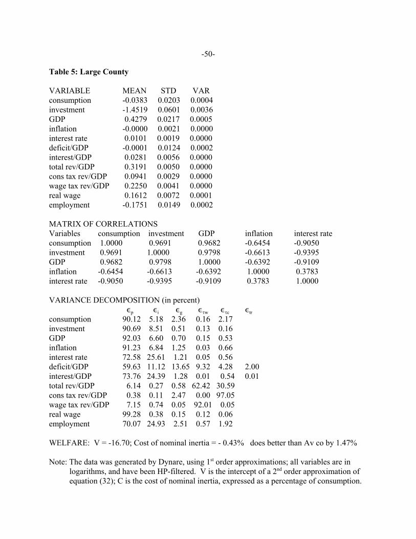
-50-
Table 5: Large County
VARIABLE MEAN STD VAR consumption -0.0383 0.0203 0.0004investment -1.4519 0.0601 0.0036GDP 0.4279 0.0217 0.0005inflation -0.0000 0.0021 0.0000interest rate 0.0101 0.0019 0.0000deficit/GDP -0.0001 0.0124 0.0002interest/GDP 0.0281 0.0056 0.0000total rev/GDP 0.3191 0.0050 0.0000cons tax rev/GDP 0.0941 0.0029 0.0000wage tax rev/GDP 0.2250 0.0041 0.0000real wage 0.1612 0.0072 0.0001employment -0.1751 0.0149 0.0002
MATRIX OF CORRELATIONSVariables consumption investment GDP inflation interest rate consumption 1.0000 0.9691 0.9682 -0.6454 -0.9050 investment 0.9691 1.0000 0.9798 -0.6613 -0.9395 GDP 0.9682 0.9798 1.0000 -0.6392 -0.9109 inflation -0.6454 -0.6613 -0.6392 1.0000 0.3783 interest rate -0.9050 -0.9395 -0.9109 0.3783 1.0000
VARIANCE DECOMPOSITION (in percent) ,p ,i ,g ,Jw ,Jc ,tr consumption 90.12 5.18 2.36 0.16 2.17investment 90.69 8.51 0.51 0.13 0.16GDP 92.03 6.60 0.70 0.15 0.53inflation 91.23 6.84 1.25 0.03 0.66interest rate 72.58 25.61 1.21 0.05 0.56deficit/GDP 59.63 11.12 13.65 9.32 4.28 2.00interest/GDP 73.76 24.39 1.28 0.01 0.54 0.01total rev/GDP 6.14 0.27 0.58 62.42 30.59cons tax rev/GDP 0.38 0.11 2.47 0.00 97.05wage tax rev/GDP 7.15 0.74 0.05 92.01 0.05real wage 99.28 0.38 0.15 0.12 0.06employment 70.07 24.93 2.51 0.57 1.92
WELFARE: V = -16.70; Cost of nominal inertia = - 0.43% does better than Av co by 1.47%
Note: The data was generated by Dynare, using 1st order approximations; all variables are in logarithms, and have been HP-filtered. V is the intercept of a 2nd order approximation of equation (32); C is the cost of nominal inertia, expressed as a percentage of consumption.

-51-
Table 6: Fiscal Rules to Reduce the Volatility of Deficit/GDP
High Debt Country
VariableNo
Response
Response in:
Wage Tax Rate Purchases
Deficit/GDP 1.46 1.00 1.00
Output 1.54 1.60 1.79
Hours Worked 1.45 1.46 1.77
Consumption 1.40 1.47 1.10
Inflation 0.39 0.40 0.36
Change in Welfare -0.55 0.56Notes:1. Results for economic variables are unconditional standard deviation, in percentages2. Results for welfare are in consumption equivalents, in percentages.
-52-
Table 7: Standard Deviations and Welfare Losses Under Alternative Transfer Schemes
Output-GapElasticity of
Transfers
0 -0.35 -0.75
SD(CO) 0.0136 0.0143 0.0150
SD(CL) 0.0189 0.0167 0.0173
SD(C) 0.0131 0.0122 0.0114
SD(I) 0.0540 0.0518 0.0503
SD(Y) 0.0165 0.0155 0.0146
SD(N) 0.0179 0.0173 0.0167
SD(W/P) 0.0079 0.0080 0.0081
SD(i) 0.0024 0.0025 0.0027
SD(Bc) 0.0042 0.0045 0.0048
SD(S/Y) 0.0121 0.0131 0.0142
Welfare Loss 0.569 1.206
Note: Standard deviations are for HP filtered variables in the model of Section 7; these figures arecalculated using the first order approximation to the model. In our benchmark specification, theelasticity of transfers with respect to the output gap is zero. The alternative specifications set thiselasticity to -0.35 and -0.75. The welfare losses of optimizing households are expressed aspercentages of their consumption, as we go from the benchmark to each alternative; these losses arecalculated using the second order approximation to the model.
-53-
Table 8A: Variance Decomposition for Benchmark Specification of Table 7.
,p ,i ,g ,tr ,Jw ,Jc CO 64.21 27.01 1.21 0.21 0.18 7.18CL 12.72 16.73 5.46 35.48 17.21 12.41C 41.45 30.46 0.70 8.57 5.76 13.06I 47.95 50.64 1.04 0.18 0.01 0.18Y 44.26 39.87 9.23 2.16 1.35 3.13N 15.73 60.92 13.52 3.18 2.03 4.63W/P 97.79 1.23 0.49 0.11 0.24 0.14i 56.56 39.85 2.63 0.45 0.08 0.43Bc 89.79 5.43 3.42 0.62 0.09 0.65S/Y 43.14 33.02 10.56 2.33 7.90 3.06
Table 8B: Variance Decomposition for Specification of Table 7 with Elasticity of - 0.75.
,p ,i ,g ,tr ,Jw ,Jc CO 68.70 24.22 0.53 0.09 0.24 6.22CL 21.36 15.42 3.85 33.07 16.55 9.75C 40.36 28.38 1.60 9.17 6.31 14.19I 47.46 51.69 0.58 0.11 0.04 0.12Y 43.94 40.18 9.17 2.18 1.33 3.21N 23.03 55.91 12.10 2.88 1.82 4.26W/P 98.21 1.11 0.32 0.07 0.19 0.09i 63.91 34.57 1.08 0.18 0.08 0.18Bc 95.30 2.48 1.57 0.29 0.06 0.31S/Y 56.80 30.07 5.04 1.16 5.31 1.61
-54-
0 10 202
4
6
8
10x 10
-3
0 10 200
0 .005
0 .01
0 .015
0 .02
0 .025inves tm en t
0 10 202
4
6
8
10x 10
-3 G D P
0 10 20-4
-3
-2
-1
0x 10
-3 in fla t ion
0 10 20-14
-12
-10
-8
-6
-4x 10
-4 in te res t ra te
0 10 20-6
-4
-2
0x 10
-3 de fic it /G D P
c ons um p t ion
0 10 20-4
-3
-2
-1
0x 10
-3
0 10 20-20
-15
-10
-5
0
5x 10
-4 to ta l rev/G D P
0 10 20-5
0
5
10x 10
-5 c ons tax rev/G D P
0 10 20-2
-1 .5
-1
-0 .5
0x 10
-3 w age tax rev/G D P
0 10 202
3
4
5
6
7x 10
-3 rea l w age
0 10 20-6
-4
-2
0
2x 10
-3 em p loy m en t
in te res t /G D P
Figure 1A: Average (Small) Country, Productivity Shock
Note: Impulse response functions generated by Dynare, using 1st order approximations.

-55-
0 10 20-8
-6
-4
-2
0x 10
-3
0 10 20-0 .03
-0 .02
-0 .01
0
0 .01inves tm en t
0 10 20-0 .01
-0 .008
-0 .006
-0 .004
-0 .002
0G D P
0 10 20-10
-5
0
5x 10
-4 in fla t ion
0 10 200
0 .5
1
1 .5x 10
-3 in te res t ra te
0 10 20-2
0
2
4
6x 10
-3 de fic it /G D P
c ons um p t ion
0 10 200
1
2
3
4
5x 10
-3
0 10 20-6
-4
-2
0x 10
-4 to ta l rev/G D P
0 10 20-5
0
5
10
15x 10
-5 c ons tax rev/G D P
0 10 20-6
-4
-2
0
2x 10
-4 w age tax rev/G D P
0 10 20-4
-2
0
2
4x 10
-4 rea l w age
0 10 20-15
-10
-5
0
5x 10
-3 em p loy m en t
in te res t /G D P
Figure 1B: Average (Small) Country, Interest Rate Shock
N o t e :Impulse response functions generated by Dynare, using 1st order approximations.

-56-
0 10 20-1 .4
-1 .2
-1
-0 .8
-0 .6x 10
-3
0 10 20-2
-1
0
1
2
3x 10
-3 inves tm en t
0 10 200
1
2
3
4x 10
-3 G D P
0 10 200
2
4
6x 10
-4 in fla t ion
0 10 201
1 .5
2
2 .5
3x 10
-4 in te res t ra te
0 10 200 .5
1
1 .5
2
2 .5
3x 10
-3 de fic it /G D P
c ons um p t ion
0 10 20-2
0
2
4
6
8x 10
-4
0 10 20-2 .5
-2
-1 .5
-1
-0 .5x 10
-4 to ta l rev/G D P
0 10 20-4
-2
0x 10
-4 c ons tax rev/G D P
0 10 200
0 .5
1
1 .5
2x 10
-4 w age tax rev/G D P
0 10 20-3 .5
-3
-2 .5
-2
-1 .5x 10
-4 rea l w age
0 10 200
1
2
3
4
5x 10
-3 em p loy m en t
in te res t /G D P
Figure 1C: Average (Small) Country, Government Purchases Shock
N o t e :Impulse response functions generated by Dynare, using 1st order approximations.
-57-
0 10 20-3
-2
-1
0x 10
-3
0 10 20-1
-0 .5
0
0 .5
1x 10
-3 inves tm en t
0 10 20-2
-1 .5
-1
-0 .5
0x 10
-3 G D P
0 10 20-3
-2
-1
0x 10
-4 in fla t ion
0 10 20-1
-0 .8
-0 .6
-0 .4
-0 .2
0x 10
-4 in te res t ra te
0 10 20-2
-1 .5
-1
-0 .5
0x 10
-3 de fic it /G D P
c ons um p t ion
0 10 20
-2
0
2x 10
-4
0 10 200
0 .5
1
1 .5
2
2 .5x 10
-3 to ta l rev/G D P
0 10 200
0 .5
1
1 .5
2
2 .5x 10
-3 c ons tax rev/G D P
0 10 20-1 .5
-1
-0 .5
0x 10
-4 w age tax rev/G D P
0 10 200
0 .5
1
1 .5
2x 10
-4 rea l w age
0 10 20-3
-2
-1
0x 10
-3 em p loy m en t
in te res t /G D P
Figure 1D: Average (Small) Country, Consumption Tax Shock
N o t e :Impulse response functions generated by Dynare, using 1st order approximations.

-58-
0 10 20-4
-3 .5
-3
-2 .5
-2x 10
-4
0 10 20-10
-8
-6
-4
-2x 10
-4 inves tm en t
0 10 20-4
-3
-2
-1x 10
-4 G D P
0 10 202
4
6
8
10x 10
-5 in fla t ion
0 10 200
2
4
6
8x 10
-5 in te res t ra te
0 10 20-4
-3
-2
-1
0x 10
-3 de fic it /G D P
c ons um pt ion
0 10 20-15
-10
-5
0
5x 10
-5
0 10 200
1
2
3
4x 10
-3 to ta l rev/G D P
0 10 20-4
-3
-2
-1
0
1x 10
-6 c ons tax rev/G D P
0 10 200
1
2
3
4x 10
-3 w age tax rev/G D P
0 10 20-5
0
5
10
15x 10
-5 rea l w age
0 10 20
-4
-2
0x 10
-4 em p loy m en t
in te res t /G D P
Figure 1E: Average (Small) Country, Labor Tax Shock
N o t e :Impulse response functions generated by Dynare, using 1st order approximations.

-59-
0 10 202
4
6
8
10x 10
-3
0 10 200
0 .005
0 .01
0 .015
0 .02
0 .025inves tm en t
0 10 202
4
6
8
10x 10
-3 G D P
0 10 20-4
-3
-2
-1
0x 10
-3 in fla t ion
0 10 20-14
-12
-10
-8
-6
-4x 10
-4 in te res t ra te
0 10 20-8
-6
-4
-2
0x 10
-3 de fic it /G D P
c ons um pt ion
0 10 20-6
-4
-2
0x 10
-3
0 10 20-20
-15
-10
-5
0
5x 10
-4 to ta l rev/G D P
0 10 20-5
0
5
10x 10
-5 c ons tax rev/G D P
0 10 20-2
-1 .5
-1
-0 .5
0x 10
-3 w age tax rev/G D P
0 10 202
3
4
5
6
7x 10
-3 rea l w age
0 10 20-6
-4
-2
0
2x 10
-3 em p loy m en t
in te res t /G D P
Figure 2A: High Debt Country, Productivity Shock
N o t e :Impulse response functions generated by Dynare, using 1st order approximations.

-60-
0 10 20-8
-6
-4
-2
0x 10
-3
0 10 20-0 .03
-0 .02
-0 .01
0
0 .01inves tm en t
0 10 20-0 .01
-0 .008
-0 .006
-0 .004
-0 .002
0G D P
0 10 20-10
-5
0
5x 10
-4 in fla t ion
0 10 200
0 .5
1
1 .5x 10
-3 in te res t ra te
0 10 20-2
0
2
4
6
8x 10
-3 de fic it /G D P
c ons um pt ion
0 10 200
2
4
6x 10
-3
0 10 20-6
-4
-2
0x 10
-4 to ta l rev/G D P
0 10 20-1
0
1
2x 10
-4 c ons tax rev/G D P
0 10 20-8
-6
-4
-2
0
2x 10
-4 w age tax rev/G D P
0 10 20-4
-2
0
2
4x 10
-4 rea l w age
0 10 20-15
-10
-5
0
5x 10
-3 em p loy m en t
in te res t /G D P
Figure 2B: High Debt Country, Interest Rate Shock
Note: Impulse response functions generated by Dynare, using 1st order approximations.
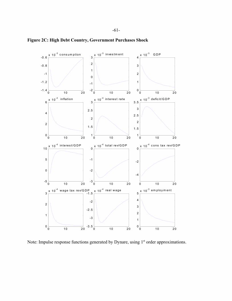
-61-
0 10 20-1 .4
-1 .2
-1
-0 .8
-0 .6x 10
-3
0 10 20-2
-1
0
1
2
3x 10
-3 inves tm en t
0 10 200
1
2
3
4x 10
-3 G D P
0 10 200
2
4
6x 10
-4 in fla t ion
0 10 201
1 .5
2
2 .5
3x 10
-4 in te res t ra te
0 10 201
1 .5
2
2 .5
3
3 .5x 10
-3 de fic it /G D P
c ons um pt ion
0 10 20-5
0
5
10x 10
-4
0 10 20-3
-2
-1
0x 10
-4 to ta l rev/G D P
0 10 20
-4
-2
0x 10
-4 c ons tax rev/G D P
0 10 200
1
2
3x 10
-4 w age tax rev/G D P
0 10 20-3 .5
-3
-2 .5
-2
-1 .5x 10
-4 rea l w age
0 10 200
1
2
3
4
5x 10
-3 em p loy m en t
in te res t /G D P
Figure 2C: High Debt Country, Government Purchases Shock
Note: Impulse response functions generated by Dynare, using 1st order approximations.
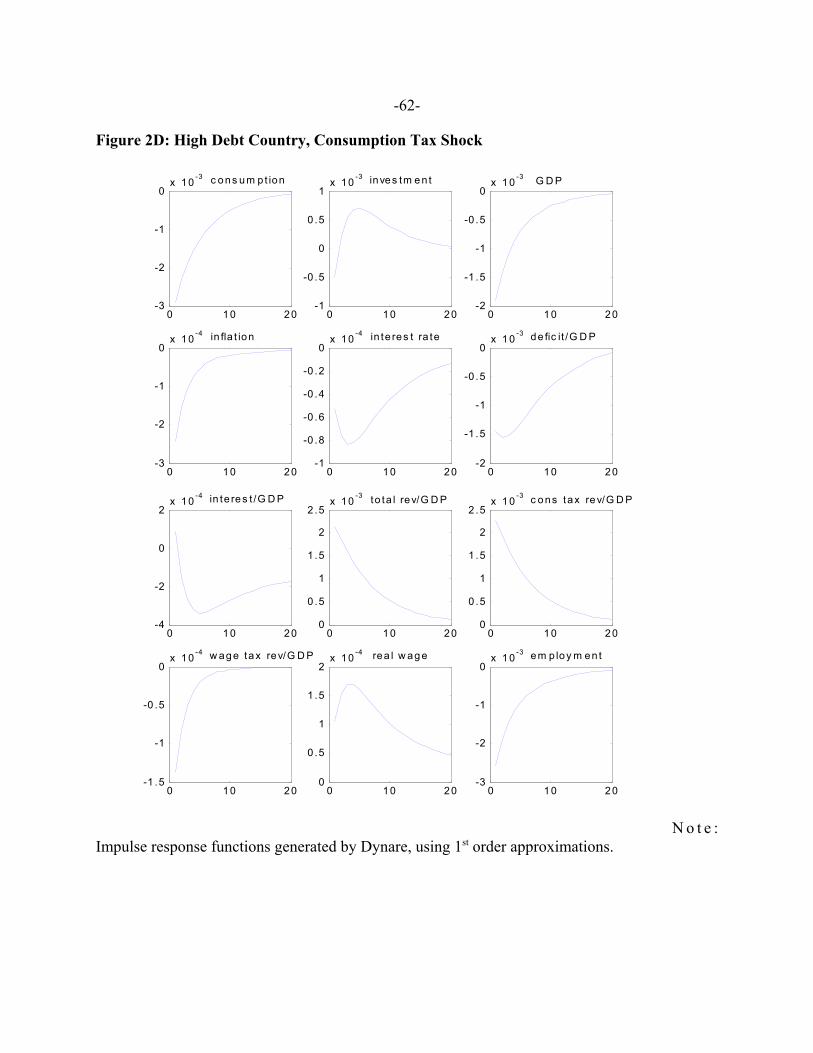
-62-
0 10 20-3
-2
-1
0x 10
-3
0 10 20-1
-0 .5
0
0 .5
1x 10
-3 inves tm en t
0 10 20-2
-1 .5
-1
-0 .5
0x 10
-3 G D P
0 10 20-3
-2
-1
0x 10
-4 in fla t ion
0 10 20-1
-0 .8
-0 .6
-0 .4
-0 .2
0x 10
-4 in te res t ra te
0 10 20-2
-1 .5
-1
-0 .5
0x 10
-3 de fic it /G D P
c ons um pt ion
0 10 20-4
-2
0
2x 10
-4
0 10 200
0 .5
1
1 .5
2
2 .5x 10
-3 to ta l rev/G D P
0 10 200
0 .5
1
1 .5
2
2 .5x 10
-3 c ons tax rev/G D P
0 10 20-1 .5
-1
-0 .5
0x 10
-4 w age tax rev/G D P
0 10 200
0 .5
1
1 .5
2x 10
-4 rea l w age
0 10 20-3
-2
-1
0x 10
-3 em p loy m en t
in te res t /G D P
Figure 2D: High Debt Country, Consumption Tax Shock
N o t e :Impulse response functions generated by Dynare, using 1st order approximations.

-63-
0 10 20-5
-4
-3
-2x 10
-4
0 10 20-12
-10
-8
-6
-4
-2x 10
-4 inves tm en t
0 10 20
-4
-2
0x 10
-4 G D P
0 10 202
4
6
8
10x 10
-5 in fla t ion
0 10 200
2
4
6
8x 10
-5 in te res t ra te
0 10 20-4
-3
-2
-1
0
1x 10
-3 de fic it /G D P
c ons um pt ion
0 10 20-1
0
1
2x 10
-4
0 10 200
1
2
3
4x 10
-3 to ta l rev/G D P
0 10 20-6
-4
-2
0
2x 10
-6 c ons tax rev/G D P
0 10 200
1
2
3
4x 10
-3 w age tax rev/G D P
0 10 20-1
0
1
2x 10
-4 rea l w age
0 10 20-6
-4
-2
0x 10
-4 em p loy m en t
in te res t /G D P
Figure 2E: High Debt Country, Labor Tax Shock
Note: Impulse response functions generated by Dynare, using 1st order approximations.
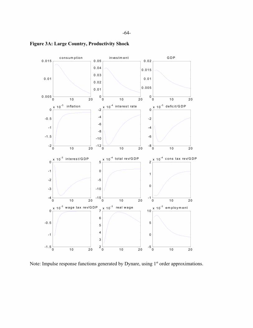
-64-
0 10 200 .005
0 .01
0 .015
0 10 200
0 .01
0 .02
0 .03
0 .04
0 .05inves tm en t
0 10 200
0 .005
0 .01
0 .015
0 .02G D P
0 10 20-2
-1 .5
-1
-0 .5
0x 10
-3 in fla t ion
0 10 20-12
-10
-8
-6
-4
-2x 10
-4 in te res t ra te
0 10 20-8
-6
-4
-2
0x 10
-3 de fic it /G D P
c ons um pt ion
0 10 20-4
-3
-2
-1
0x 10
-3
0 10 20-15
-10
-5
0
5x 10
-4 to ta l rev/G D P
0 10 20-1
0
1
2x 10
-4 c ons tax rev/G D P
0 10 20-1 .5
-1
-0 .5
0x 10
-3 w age tax rev/G D P
0 10 202
3
4
5
6
7x 10
-3 rea l w age
0 10 20-5
0
5
10x 10
-3 em p loy m en t
in te res t /G D P
Figure 3A: Large Country, Productivity Shock
Note: Impulse response functions generated by Dynare, using 1st order approximations.

-65-
0 10 20-5
-4
-3
-2
-1
0x 10
-3
0 10 20-20
-15
-10
-5
0
5x 10
-3 inves tm en t
0 10 20-6
-4
-2
0x 10
-3 G D P
0 10 20-6
-4
-2
0
2x 10
-4 in fla t ion
0 10 200
0 .2
0 .4
0 .6
0 .8
1x 10
-3 in te res t ra te
0 10 20-1
0
1
2
3
4x 10
-3 de fic it /G D P
c ons um pt ion
0 10 200
1
2
3x 10
-3
0 10 20-3
-2
-1
0
1x 10
-4 to ta l rev/G D P
0 10 20-5
0
5
10x 10
-5 c ons tax rev/G D P
0 10 20-4
-2
0
2x 10
-4 w age tax rev/G D P
0 10 20-4
-2
0
2
4x 10
-4 rea l w age
0 10 20-8
-6
-4
-2
0
2x 10
-3 em p loy m en t
in te res t /G D P
Figure 3B: Large Country, Interest Rate Shock
Note: Impulse response functions generated by Dynare, using 1st order approximations.

-66-
0 10 20-2 .5
-2
-1 .5
-1
-0 .5x 10
-3
0 10 20-4
-3
-2
-1
0x 10
-3 inves tm en t
0 10 200
0 .5
1
1 .5
2x 10
-3 G D P
0 10 200
1
2
3x 10
-4 in fla t ion
0 10 200 .5
1
1 .5
2x 10
-4 in te res t ra te
0 10 200
1
2
3
4x 10
-3 de fic it /G D P
c ons um p t ion
0 10 20-2
0
2
4
6
8x 10
-4
0 10 20-3
-2
-1
0x 10
-4 to ta l rev/G D P
0 10 20-4
-2
0x 10
-4 c ons tax rev/G D P
0 10 200
0 .2
0 .4
0 .6
0 .8
1x 10
-4 w age tax rev/G D P
0 10 20-3
-2 .5
-2
-1 .5
-1x 10
-4 rea l w age
0 10 200
0 .5
1
1 .5
2
2 .5x 10
-3 em p loy m en t
in te res t /G D P
Figure 3C: Large Country, Government Purchases Shock
Note: Impulse response functions generated by Dynare, using 1st order approximations.

-67-
0 10 20-3
-2
-1
0
1x 10
-3
0 10 200
0 .5
1
1 .5
2x 10
-3 inves tm en t
0 10 20-15
-10
-5
0
5x 10
-4 G D P
0 10 20-2
-1 .5
-1
-0 .5
0x 10
-4 in fla t ion
0 10 20-1 .5
-1
-0 .5
0x 10
-4 in te res t ra te
0 10 20-2
-1 .5
-1
-0 .5
0x 10
-3 de fic it /G D P
c ons um pt ion
0 10 20-4
-2
0
2x 10
-4
0 10 200
0 .5
1
1 .5
2
2 .5x 10
-3 to ta l rev/G D P
0 10 200
0 .5
1
1 .5
2
2 .5x 10
-3 c ons tax rev/G D P
0 10 20-1
-0 .8
-0 .6
-0 .4
-0 .2
0x 10
-4 w age tax rev/G D P
0 10 200 .8
1
1 .2
1 .4
1 .6x 10
-4 rea l w age
0 10 20-2
-1 .5
-1
-0 .5
0x 10
-3 em p loy m en t
in te res t /G D P
Figure 3D: Large Country, Consumption Tax Shock
Note: Impulse response functions generated by Dynare, using 1st order approximations.
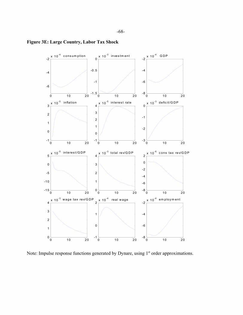
-68-
0 10 20
-6
-4
-2x 10
-4
0 10 20-1 .5
-1
-0 .5
0x 10
-3 inves tm en t
0 10 20-8
-6
-4
-2x 10
-4 G D P
0 10 20-1
0
1
2
3x 10
-5 in fla t ion
0 10 20-1
0
1
2
3
4x 10
-5 in te res t ra te
0 10 20-3
-2
-1
0x 10
-3 de fic it /G D P
c ons um pt ion
0 10 20-15
-10
-5
0
5x 10
-5
0 10 200
1
2
3
4x 10
-3 to ta l rev/G D P
0 10 20-8
-6
-4
-2
0
2x 10
-6 c ons tax rev/G D P
0 10 200
1
2
3
4x 10
-3 w age tax rev/G D P
0 10 20-1
0
1
2x 10
-4 rea l w age
0 10 20-8
-6
-4
-2x 10
-4 em p loy m en t
in te res t /G D P
Figure 3E: Large Country, Labor Tax Shock
Note: Impulse response functions generated by Dynare, using 1st order approximations.

-69-
Figure 4A: Model with Non-Optimizers, Transfer Shock
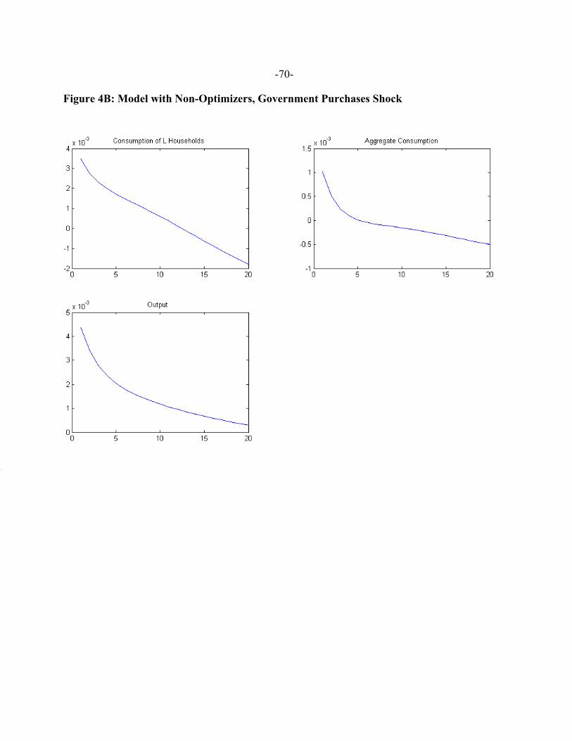
-70-
Figure 4B: Model with Non-Optimizers, Government Purchases Shock