Embed Size (px)
Citation preview

NBER WORKING PAPER SERIES
DO ASSET PRICES REFLECT FUNDAMENTALS?FRESHLY SQUEEZED EVIDENCE FROM THE OJ MARKET
Jacob BoudoukhMatthew Richardson
YuQing ShenRobert F. Whitelaw
Working Paper 9515http://www.nber.org/papers/w9515
NATIONAL BUREAU OF ECONOMIC RESEARCH1050 Massachusetts Avenue
Cambridge, MA 02138February 2003
We would like to thank Kent Daniel (NBER discussant), Murray Frank, Owen Lamont, Tom Miller(WFA discussant), Richard Roll, Bill Silber, Jeff Wurgler and seminar participants at the Federal ReserveBoard of Governors, Washington D.C., Princeton University, Rice University, Tel-Aviv University,UCLA, UBC, the NBER summer institute, the Western FinanceAssociation meetings, University ofRochester, and New York University for their valuable comments. Contact: Prof. R. Whitelaw, NYU,Stern School of Business, 44 W. 4th St., Suite 9-190, New York, NY 10012, (212) 998-0338,[email protected] views expressed herein are those of the author and not necessarily those ofthe National Bureau of Economic Research.
©2003 by Jacob Boudoukh, Matthew Richardson, YuQing Shen, and Robert F. Whitelaw. All rightsreserved. Short sections of text not to exceed two paragraphs, may be quoted without explicit permissionprovided that full credit including ©notice, is given to the source.

Do Asset Prices Reflect Fundamentals? Freshly Squeezed Evidence from the OJ MarketJacob Boudoukh, Matthew Richardson, YuQing Shen, and Robert F. Whitelaw NBER Working Paper No. 9515February 2003JEL No. G1
ABSTRACT
The behavioral finance literature cites the frozen concentrated orange juice (FCOJ) futuresmarket as a prominent example of the failure of prices to reflect fundamentals. This paperreexamines the relation between FCOJ futures returns and fundamentals, focusing primarily ontemperature. We show that when theory clearly identifies the fundamental, i.e., at temperatures closeto or below freezing, there is a close link between FCOJ prices and that fundamental. Using asimple, theoretically-motivated, nonlinear, state dependent model of the relation between FCOJreturns and temperature, we can explain approximately 50% of the return variation. This is importantbecause while only 4.5% of the days in winter coincide with freezing temperatures, two-thirds ofthe entire winter return variability occurs on these days. Moreover, when theory suggests no suchrelation, i.e., at most temperature levels, we show empirically that none exists. The fact that thereis no relation the majority of the time is good news for the theory and for market efficiency, not badnews. In terms of residual FCOJ return volatility, we also show that other fundamental informationabout supply, such as USDA production forecasts and news about Brazil production, generatesignificant return variation that is consistent with theoretical predictions. The fact that, even in thecomparatively simple setting of the FCOJ market, it is easy to erroneously conclude thatfundamentals have little explanatory power for returns serves as an important warning to researcherswho attempt to interpret the evidence in markets where both fundamentals and their relation to pricesare more complex.
Jacob Boudoukh Matthew RichardsonIDC, Arison School of Business NYU, Stern School of Business Visiting Stern-NYU 44 W. 4th St. 44 W. 4th St. New York, NY 10012New York, NY 10012 and NBERand NBER [email protected]@stern.nyu.edu
Jeffrey (YuQing) Shen Robert F. Whitelaw JP Morgan Fleming Asset Management NYU, Stern School of Business 522 Fifth Ave 44 W. 4th St. New York, NY 10036 New York, NY [email protected] and NBER

1 Introduction
There has been considerable research that investigates whether asset prices reflect their fundamental
values.1 The general conclusion from this research is that the variability of returns is much greater
than that implied by the assets’ fundamentals, i.e., information about the asset’s cash flows and
expected returns. Specifically, regressions of asset returns on ex post information (relevant for
pricing the assets) reveals little explanatory power.
Explanations for the empirically documented lack of a relation between asset returns and fun-
damental news can be found in the growing literature in behavioral finance. For example, DeLong,
Shleifer, Summers, and Waldmann (1990, p.724-726) explicitly cite the above evidence as support
for their noise trading model. It seems premature, however, to view this evidence as definitive.
There is the alternative explanation that the relation between asset prices and fundamental in-
formation is incorrectly measured or not measured at all (e.g., omitted variables).2 We provide
supportive evidence favoring this latter view by analyzing a market where existing empirical re-
sults have been interpreted as being consistent with market irrationality, and to illustrate how
looking at the data in a new way can potentially overturn this interpretation. By necessity, we
choose an example where at least some of the relevant fundamental information is easy to identify,
and where theory provides strong intuition about the functional form of the relation between fun-
damentals and returns. The fact that, even in this simple setting, it is easy to erroneously conclude
that fundamentals have little explanatory power for returns is an important warning to researchers
who attempt to interpret the evidence in markets where both fundamentals and their relation to
prices are more complex.
Our example comes from one of the forerunners of the excess volatility literature–Roll’s (1984)
seminal paper on frozen concentrate orange juice (FCOJ) futures prices and weather. His paper is
unique and clever in that the fundamental information appears to be identifiable and exogenous.
A critical aspect of this market is that the relevant oranges for FCOJ are produced in a relatively1For example, see Shiller (1981), Meese and Rogoff (1983), Black (1986), Campbell and Shiller (1987), Frankel
and Meese (1987), Roll (1988), Cutler, Poterba and Summers (1989), Lev (1989), and Mitchell and Mulherin (1994)
to name just a few.2Moreover, the research design of some of these previous studies have been put into question, examples of which
include Kleidon’s (1986) analysis of Shiller’s (1981) excess volatility paper, or, more recently, Fama’s (1998) criticism
of so-called anomalies in the corporate event study literature.
1

small region of Florida. Thus, as Roll (1984) reasonably argues, the weather in this region should
be a primary determinant of supply and thus of futures prices. Roll (1984, p.876) states that
“weather is the most identifiable factor influencing FCOJ returns”; however, overall, he finds little
explanatory power in the relation between FCOJ futures prices and weather. In his conclusion,
Roll (1984, p.879) states that
...weather surprises explain only a small fraction of the observed variability in futures
prices. The importance of weather is confirmed by the fact that it is the most frequent
topic of stories concerning oranges in the financial press and by the ancillary fact that
other topics are associated with even less price variability than is weather... There is a
large amount of inexplicable price volatility.
Weather’s apparent lack of explanatory power for FCOJ returns has become a popular citation
in the behavioral literature precisely because the fundamental information seems to be so clear.
However, it is important to note that while Roll’s findings have subsequently been adopted by the
excess volatility literature, at the time, the paper was seen in many ways as being supportive of
market efficiency in that it also focused on how prices rationally incorporate all the information
in weather forecasts. Moreover, while Roll identifies the puzzling lack of explanatory power, he
does not argue that this evidence implies market irrationality. Nevertheless, in recent surveys of
behavioral finance
• Shleifer (2000, p.20), in a discussion about empirical challenges to efficient markets, asks
“what about the basic proposition that stock prices do not react to non-information? Here
again there has been much work, but three types of findings stand out... many sharp moves
in stock prices do not appear to accompany significant news... A similar conclusion has been
reached in two striking studies by Richard Roll (1984, 1988)...He finds that, although news
about weather helps determine future price movements, they account for a relatively small
share of these movements”;
• Hirshleifer (2001, p.1560) writes in a section covering mispricing effects that “little of stock
price or orange futures price variability has been explained empirically by relevant public
news”;
2

• Ross (2001, p.11) argues that “the regressions themselves have low power even when run
with the return as the dependent variable and past returns and weather forecasts as well as
contemporaneous weather changes. The R2 of these regressions is on the order of 1 or 2%. In
other words, while there is no evidence that prices do not fully incorporate past information,
we are pretty much at a loss to say why they move at all! If it’s not weather - which is
obviously the biggest determinant of supply changes - then what could it be?”;
• Daniel, Hirshleifer and Teoh (2002, p.172) state “only a small fraction of stock prices or
orange juice futures prices has been explained by the arrival of relevant public news. Roll
(1984) finds that the volatility of OJ futures prices was hard to explain by news about the
weather”.
In this paper, we show that this literature has misinterpreted the data by ignoring the state
dependence inherent in the structural relation between FCOJ returns and their underlying fun-
damentals. In particular, the identified fundamental, i.e., weather surprises, should theoretically
impact FCOJ futures returns only in one state of nature, namely to the extent this surprise pro-
vides the market with some new information about the probability and severity of a freeze. The
implication of this is that most weather surprises should have no impact at all. For example, an
unexpected 30 degree drop in temperature from 80 to 50 degrees in late December might affect the
tourism industry in Orlando, but it will have no impact on the FCOJ market. In contrast, a much
smaller unexpected 5 degree drop from 30 to 25 degrees will have devastating effects on the Florida
orange crop.
We document that in most circumstances, as theory would predict, the R2 is zero between
FCOJ futures returns and weather changes. However, around freezing temperatures, the only state
of nature that theoretically matters, we estimate R2s on the order of 50% using a variety of (albeit
rudimentary) models and information. This difference in R2 is nontrivial. In fact, over one-half of
all variation of FCOJ returns occurs in the winter season. Of this variation, two-thirds occurs on
just 4% of the days. Not surprisingly, these days are not random and are instead related to freezing
temperatures. There is only conclusion that can be drawn from these results - there is absolutely
no puzzle concerning the relation between FCOJ prices and the weather.
There is, of course, variation of FCOJ returns in other seasons when there is little or no in-
formation about the possibility of freezing temperatures. However, the fact that FCOJ prices
3

vary throughout the year should come as no surprise to agricultural economists; this is true of all
commodity prices (see, for example, Fleming, Kirby and Ostdiek (2002)). Whether the remaining
volatility can be explained by information about demand for OJ, or futures-specific issues such as
the microstructure of the market or the commodity’s convenience yield, is difficult to determine.
Nevertheless, we focus on other non-weather related news about supply-side shocks to the FCOJ
market and identify three important sources: (i) USDA production forecasts, (ii) resolution of
production uncertainty, and (iii) production from areas outside of Orlando, the majority of which
comes from Brazil. Theory suggests that all of these sources should generate news that is important
for FCOJ prices, and the evidence confirms this. For example, each year in mid-October the United
States Department of Agriculture (USDA) provides its initial forecast of orange production for the
season. Over 40% of total fall FCOJ futures return variance occurs on that day. This fact alone
suggests that the market does not ignore fundamental information about production independent
of the weather effect.3 Together, the October production forecast days and freezing temperature
days account for 1.5% of the days in our sample. On these days 41% of total FCOJ return variance
is observed. This is apparently not a market in which investors are ignoring public fundamental
information.
The paper is organized as follows. In Section 2, we provide the theory for how FCOJ prices
should be related to supply shocks, and, in particular, weather. Of particular interest, we shed light
on why the literature has misinterpreted the existing findings. Section 3 describes the data and
the basic stylized facts about weather, production and FCOJ futures prices. This section provides
strong circumstantial evidence that these three variables are linked. In Section 4, we then test these
links more formally, and, in general, confirm the theoretical relation empirically. In particular, there
is close relation between FCOJ prices and temperature when the theory suggests there should be
one. Section 5 explores the fact that there is remaining volatility in FCOJ prices not explained
by the weather. In particular, we explore the effect of other factors on FCOJ prices. Section 6
concludes.3Bauer and Orazem (1994) examine USDA forecasts, showing that forecast surprises provide information that is
relevant for FCOJ pricing. They report R2s for the initial October forecast day that are similar in magnitude to
those we report for freeze days.
4

2 Theory of FCOJ and Weather
There is a growing literature in finance arguing that asset prices drift away from their underlying
fundamentals due to irrational agents who ignore these fundamentals. This literature is motivated,
at least in part, by empirical evidence documenting a disconnect between fundamentals and asset
prices. For example, the empirical literature reports low R2s from linear regressions of returns
on unexpected changes in the fundamentals. However, these regressions measure the linear, state
independent, relation between innovations to the fundamentals and asset returns, and attempting to
link asset returns to changing fundamentals in such an atheoretical framework can be problematic.
Asset pricing models often result in a complex structural relation between fundamentals and prices;
therefore, linear regressions ignore state dependence and nonlinearity that occur quite naturally.
This paper addresses the problematic nature of drawing economically meaningful conclusions
from these types of empirical models in the context of the FCOJ market. The FCOJ market is
a natural choice because it has generated considerable attention, not least because it seems to
provide such a strong case for irrationality. What are the fundamental determinants of prices in
this market? First, and foremost, there are short-run shocks to the Florida-based production of
oranges,4 which are primarily attributable to the weather. Second, due to worldwide production
of oranges suitable for FCOJ, unexpected changes in the ability of distributors to shift away from
Florida oranges to other sources also affects returns. In particular, Brazil is the largest exporter
of oranges worldwide and thus news about production in Brazil is relevant for the price of FCOJ.
Finally, there could be short-run demand shifts either to or away from FCOJ. Competing products
include other citrus juices, such as grapefruit juice, lemonade or freshly squeezed orange juice,
and other fruit juices such as apple juice. The fact that companies spend considerable amounts
marketing FCOJ products provides anecdotal evidence that demand matters.
Thus, relative to other markets, the FCOJ market appears to be less complicated. Of equal
importance, the primary fundamental factor, namely weather, is clearly exogenous. No one believes
FCOJ prices have any affect on weather patterns in Orlando, Florida. It is this combination of
features that should provide a clean environment for examining the relation between asset prices4In fact, because storage costs of oranges and, in particular, FCOJ are high, only a fraction of the juice gets
carried forward from year-to-year. Therefore, long-run shifts in either demand or supply, are expected to have little
impact on FCOJ prices.
5

and fundamentals.
Outside of the fundamental determinants of FCOJ prices, there may be additional factors that
affect FCOJ returns. However, since it is not our goal in this paper to explain all the movement in
prices, but rather to demonstrate that relevant information about fundamentals gets incorporated
into prices, we ignore a lot of return-relevant information. In particular, we ignore well known fac-
tors that affect returns including microstructure effects (e.g., liquidity and the bid-ask spread), the
role of stochastic convenience yields, variations in storage costs, stochastic interest rates, delivery
costs and so forth, which are covered elsewhere in the literature.
There are several reasons why a simple linear model cannot provide a sufficiently rich framework
to address the question of whether asset returns incorporate information on fundamentals efficiently
in the context of the FCOJ market. Specifically,
• The relation between FCOJ returns and weather surprises depends on the existing state.
• There is a nonlinear relation between FCOJ returns and weather.
• The realization of the expected temperature (i.e., a zero forecast error) is itself news.
The following three subsections elaborate on these issues.
2.1 State Dependence
Roll (1984) performs three analyses by looking at the relation between FCOJ futures returns and
(i) temperature surprises, (ii) rainfall forecast errors, and (iii) a variety of explanatory variables in-
cluding temperatures, exchange rate changes, and stock returns. Proponents of market irrationality
focus their attention on some of the results related to (i). With respect to temperature surprises
(the difference between realized temperatures and forecasts), Roll documents a statistically signif-
icant relation, but finds R2s between 1% and 4%. Returns are informationally efficient in that
forecast errors are not related to future returns, which is arguably the focus of his analysis, but the
explanatory power is minimal. Based on these results, Roll concludes that “the small predictive
power for temperature and rainfall seems to imply that influences other than weather are affecting
OJ returns” (p.875). It is empirical evidence and statements such as these that have been inter-
preted by other researchers as indicating a lack of explanatory power for fundamentals in the FCOJ
futures market.
6

However, the relation between returns and weather surprises depends critically on the existing
state. That is, the conventional view in the FCOJ market is that it is only freezing temperatures
that produce supply shocks. Thus, theory implies that the weather surprise is only relevant to the
extent it tells us something about the change in likelihood and magnitude of a freeze.
There are several obvious ways to incorporate state dependence. First, freezes are seasonal –
fall, spring and summer months are unlikely to produce freezing weather in Florida.5 Second, a
temperature surprise, or change in temperature, will only matter around freezing temperatures.
That is, a 10-degree surprise at 70 degrees has very different implications for the likelihood and
severity of a freeze than it does at a temperature of 35 degrees. Even during winter, at most
temperature levels, theory tells us that there is no relation between FCOJ prices and temperature.
Third, the distribution of the freeze-related supply shock will depend on whether there has already
been a freeze during the same growing season. For example, if a freeze has a substantial impact
on orange production, then a second freeze may have less impact to the extent that the damage
is already done. Of course, this depends on the relative severity of the freezes, the timing of the
harvests, etc. In addition, conditional on a freeze, the uncertainty regarding its effects on production
can be quite high until the damage is surveyed. Any analysis of R2s that does not take these state
dependencies into account is flawed.6
2.2 Nonlinearity
A second obvious improvement to the linear specification is to allow the unexpected change in the
fundamental to be nonlinearly related to the asset return (controlling for the state dependence5Roll attempts to adjust for the importance of freezes by giving greater weight to observations in winter, but this
correction is inadequate to capture the degree of state dependence in the data. In particular, we will argue that the
weight on non-winter data must be zero by theory.6In this paper, we do not look at the relation between the FCOJ market and rainfall. Similar to temperature
surprises, however, Roll runs a regression on rainfall forecast errors and finds no discernible relation to returns. With
respect to rainfall, Roll acknowledges that its effect “on the crop is much less obvious than the effect of temperature”
(p.873). For example, either too little or too much rainfall can have a negative impact on OJ production and
quality. Moreover, only extended periods of too little or too much rain are likely to have a significant effect, and the
magnitude of the effect will depend on the timing relative to the growing season. Thus, the analysis with rainfall is
also suspect in terms of interpreting R2s due to the presence of similar state dependence and nonlinearity as observed
with temperature.
7

as discussed above). In practice, the severity of a freeze depends on two factors: (i) the level of
the temperature, and (ii) the duration of a freeze. Table 1 provides a brief description of these
relevant factors. In particular, the severity of a freeze is not linear in temperature, as 30-31 degree
temperatures have relatively mild effects compared to temperatures in the 27-29 degree range. In
the latter instance, there is severe damage done to both the leaves and fruit, which dramatically
affects production. Thus, at freezing levels, as temperatures drop just a degree or two, the supply
shock gets worse at an accelerating rate. On the other hand, at levels much below freezing, another
degree or two will not make a difference. The effect of ignoring the nonlinearity will again be to
lower the R2s in the regression analysis.
2.3 News When Forecasts are Correct
Implicit in a regression of asset returns on forecast errors is the assumption that a zero forecast
error (i.e., the realization of the expectation) should have no effect. While this holds for a linear
relation between prices and fundamentals, it does not hold generally. Consider a scenario under
which the market forecasts a freezing temperature but with some uncertainty. In other words,
the expected minimum temperature tomorrow is below freezing, but, given the difficulties inherent
in weather forecasting, there is a significant probability the temperature will be higher or lower.
The full distribution of possible future temperatures is incorporated in the price of FCOJ futures
today. In particular, today’s price reflects the probability that there will be no freeze tomorrow, no
supply shock and therefore no impact on prices. When the freeze is realized (and let us suppose at
the forecasted minimum temperature so that the “weather surprise” is zero), there is an obvious
shift in the likelihood of a freeze. Invariably, returns will increase in this instance even though the
forecast error is zero. Of course, ignoring this fact leads to lower R2s for FCOJ returns and in other
cases in which asset returns are linked to “surprises” in the fundamentals, as long as there is state
dependence or nonlinearity in the relation.
While Roll (1984) does not explicitly address the importance of this possibility in his analysis,
he does report results from a regression of returns on a temperature freeze variable and seven
other variables including exchange rates, oil prices and stock returns (see Roll (1984), Table 10 in
a section entitled “Nonweather Influences on OJ Prices”). Though we take issue with the exact
form of the specification, the identification of the freeze variable is very close to identification of
8

the relevant fundamental. This is because the freeze variable captures both the state dependence
described in Section 2.1 above and the realization versus expectation issue described here. Not
surprisingly, the explanatory power of this regression is greater, although the R2 is still only 6.7%.
This low R2 derives from (i) treating all observations the same (e.g., running the regression across all
seasons), (ii) not incorporating temperature forecasts, (iii) ignoring nonlinearities between weather
and returns, and (iv) ignoring limit price moves (in contrast to Roll’s earlier tables). Thus, it is
perhaps not surprising that the existing behavioral literature has drawn the wrong inference from
these results.
3 Data
Futures contracts in frozen concentrated orange juice (FCOJ) have traded on the New York Cotton
Exchange since September of 1967. At any given time, there are usually nine to eleven contracts
outstanding with expiration schedules every second month (January, March, May, etc.) and with
at least two January months listed at all times. The contract is for 15,000 pounds of frozen
concentrated orange juice, which represents about 2,400 ninety-pound field boxes of oranges, with
specific requirements for color, favor, and defects. Due to these requirements, 95% of the total U.S.
processed orange production takes place in central Florida in and around the Orlando area.7 There
are two types of oranges produced in the Orlando area with the main distinction being the harvest
period, namely early and mid-season (EM) varietals and Valencia oranges, which get harvested
from November through March (though primarily in January) and April though June, respectively.
The geographic concentration in orange juice production is somewhat unique for agricultural
commodities, and allows us to study the interaction between asset returns (i.e., FCOJ futures prices)
and an important exogenous variable (i.e., Orlando weather). Ex ante there are strong reasons why
weather should be an important variable for FCOJ prices and why Roll’s (1984) result is such a
puzzle. In particular, freezes can have devastating effects on orange production. Attaway (1997)7California is also a large producer of oranges; however, oranges produced in that region are not suitable for FCOJ.
Internationally, Brazil is, along with the U.S., the largest producer of oranges used for FCOJ. While Brazil primarily
exports these oranges to countries other than the U.S., the majority of Florida production is consumed domestically.
Though Brazilian oranges are subject to significant tariffs, they can provide a close substitute to Florida oranges.
The issue of Brazil’s production and how it affects the FCOJ market is discussed in Section 5.2.
9

cites several freezes over the past 170 years that have had a major impact on fruit production. A
full list of the impact freezes is provided in Table 2. For example, during the freeze of February
7-9, 1835, temperatures dropped to as low as 11 degrees in northern Florida, destroying almost all
existing orange trees. In fact, prior to this date, a number of more northern states (such as South
Carolina and Georgia) produced oranges. The freeze of 1835 essentially forever ended the desire to
produce oranges in those states. In the decade from 1894 to 1905, Florida was hit by ten freezes,
one of which (February 8, 1895 when the temperature reached 17 degrees) led to almost all the
orange crop being destroyed. In 1893-94, 5.06 million boxes of oranges were produced; by 1895-96,
production had fallen to 0.147 million boxes (Attaway (1997)). The industry did not fully recover
until 1909-10. Of interest to this paper, Table 2 shows that a number of freezes occurred during
our sample period, that is, post 1967.
We collected data from September 1967 to December 1998 on several series: (i) the minimum
temperature in Orlando, (ii) a limited amount of minimum temperature forecasts from the National
Weather Service (primarily for winter months and for only some of the years within our sample),
(iii) USDA production forecasts, and (iv) FCOJ futures prices, volume and open interest on every
contract. We also collected other relevant data series such as Brazilian orange production and
FCOJ exports to the U.S., and news events associated with FCOJ. We describe the data in detail
as it becomes relevant throughout the paper.
3.1 Orlando Weather
The most important fundamental for FCOJ prices is the presence of a production shock to a given
year’s orange crop. The largest factor in this regard is weather, and, in particular, winter freezes.
As mentioned above, winter freezes can severely impact orange production, thus raising the prices
of oranges in the commodity market.
Figure 1 graphs the minimum temperature in Orlando, Florida from 1967 through the end of
1998. Over 80% of the winter years include one or more days with temperatures close to or below
freezing during periods relevant for orange juice production. Specifically, within our sample period
of thirty-one winters, only six winters can be strictly described as completely freeze-free winters.
Twenty-five winters experienced one or more nights when the minimum temperature dipped to 32
degrees or below. Approximately 50% of the winters have two to three nights of freeze, and the
10

probability of four or more freeze nights is approximately 25%. Thus, there is clearly a considerable
amount of price-relevant information during the winter season.
However, it is important to point out that not every freeze has material consequences for the
orange crop. As mentioned above, Attaway (1997) provides a detailed description of the history
of impact freezes that happened in Florida. While Table 2 documents the actual dates of these
freezes, recall that Table 1 describes the critical conditions for freezes to have a substantial effect
on production. These conditions are essentially the temperature itself and the duration of this
temperature level.8 For example, if the temperature falls below 28 degrees for six hours or more,
then, without intervention, oranges will suffer extensive damage, hence affecting production of
FCOJ. With respect to our particular sample period, according to Attaway (1997), there are eleven
relevant freeze seasons, some of which have multiple freezes, from 1967 to 1998.9 The identification
of these freezes will form the basis for our comparison between freeze and non-freeze years.
3.2 Production
Every October, the United States Department of Agriculture (USDA) provides forecasts of the
upcoming season’s orange production. This forecast is conditioned on a non-freeze season, that is,
the USDA does not take into account the possibility of a freeze when forming its forecast.
Table 3 documents the percentage difference between the October USDA forecast and final
production, which is generally reported in August of the following year, for all the years in our
30-year sample. Freeze years, as classified by Attaway (1997), are noted, and we also report the
average across the 11 freeze years and 19 non-freeze years. Several observations are of interest.
First, the USDA’s forecasts in non-freeze years are nearly unbiased, with only a 1.3% difference on
average between the forecast and the realization. However, there is substantial variation in forecast
accuracy, with underestimates and overestimates as large as 6.2% and 8.1%, respectively. Second,
and most important, there is a considerable reduction in orange production in freeze years, with8Of course, the magnitude of a freeze alone is not sufficient to explain the impact on prices. Also important are
coincidental effects on the determinants of the supply of Florida FCOJ substitutes such as imported FCOJ from
Brazil. Examples of these effects are whether there was a drought in the Sao Paolo area of Brazil, tariff rates, and
the costs of transportation.9In a separate study by Hebert (1993), similar freezes are also identified using a different freeze identification
methodology.
11
12.7% less production than forecast. Again, there is substantial variation, with a maximum decline
of 30.5%. If the demand for oranges is downward sloping and there is no perfect substitute for
Florida oranges (at the prevailing price), then the spot price of oranges should rise in response to
a decline in supply. Given the economic laws of supply and demand, therefore, futures prices on
FCOJ should move in the same direction.
3.3 Futures Prices
In order to investigate the effect of freezes on prices, we obtained daily closing prices of FCOJ
futures from September 1967 to August 1998. On each trading day prices of the three near maturity
contracts were collected from Bridge/CRB and Datastream. We also collected volume and open
interest data. There are a number of ways to generate a continuous return series from the three
price series. In general, we attempt to get the most accurate proxy for price changes in spot FCOJ
prices. We need to take into consideration two important characteristics of futures’ prices that may
affect the accuracy of calculated returns – liquidity and limit days. First, it is well known that near
maturity contracts are the most liquid, a fact that we verified with the volume and open interest
data. However, liquidity diminishes rapidly as a contract comes close to expiration, particularly in
the expiration month. These factors were considered in constructing the continuous return series.
A second issue is that price moves on futures contracts are limited by the exchange. The magnitude
of these price limits and the contracts to which they applied change over the course of our sample,
but the general impact of price limits is to prevent prices from fully incorporating information on
days with important information releases. We adjust for this phenomenon in the standard way by
aggregating returns over consecutive days with price moves that hit either the lower or upper limit.
For example, when a severe freeze occurs, the price may hit the upper limit for 4 consecutive days.
In this case, we aggregate returns over these 4 days plus the next day, which is a no-limit day, and
use this as the 1- day return. The precise algorithm we use to construct the spliced data series is
described in the appendix.
Given this continuous daily return series, Table 3 provides the cumulative return over the winter
season (December through February) for each year and the average of these returns for freeze and
non-freeze years. The average return is almost 19% higher in freeze years than in non-freeze years,
namely 12.7% versus - 6.1%, although there is substantial variation in returns on an annual basis.
12

This suggests that, on average, futures prices are indeed higher in years in which production has
been impacted negatively.
It is also worthwhile documenting some additional stylized facts that provide substantial cir-
cumstantial evidence of an important relation between FCOJ futures prices and temperature. Table
4, Panel A reports the volatility of daily FCOJ returns in different seasons. The variance of FCOJ
futures returns in winter months is four times that of returns in spring and summer months and
three times higher than in the fall season. This is not surprising as freezes only occur in winter
months. A slightly different way of viewing the data is to note that more than 50% of the total
variance of returns is accounted for by the winter season. If the mean returns are the same across
different categories, as they are approximately across seasons, this variance decomposition can be
calculated simply by multiplying the daily variance by the number of observations in any season.
We also divided the winter season into two separate periods: pre-freeze and post-freeze. The
pre-freeze period includes days up to and including the first freeze of the season in a freeze season
and all the days in a non-freeze season; the post-freeze period includes the days subsequent to a
freeze in a freeze season. Note that the post-freeze period can include a second freeze, and, in fact,
two seasons had multiple freezes (see Table 2).
Interestingly, the variability in winter months is greater pre-freeze than post- freeze in spite of
the fact that freeze frequencies are similar in the two periods. Of course, this phenomenon may
be due to the fact that the second freeze in a season happened to be less severe in our sample.
Alternatively, the second freeze in a season may be less important because damage has already
been done to the orange crop. Due to uncertainty surrounding the impact of multiple freezes, the
remainder of the paper focuses on the period up to and including the first freeze of the season, i.e.,
the pre-freeze period.
The fact that winter months produce greater variation in futures prices does not in itself suggest
a relation between temperature and FCOJ prices. As shown in Tables 1 and 2, the main impact on
production comes from a particular event, namely a freeze. Thus, it is the change in the likelihood
of a freeze that should move FCOJ futures prices. Table 4, Panel B presents the volatility of FCOJ
futures prices in winter months conditional on various contemporaneous minimum temperature
realizations, namely 35 degrees and below, 36-40 degrees, 41-45 degrees and 46 degrees and above.
As can be seen from the table, at or around freezing temperatures (i.e., 35 and below), the
13

daily standard deviation of FCOJ returns is 11.81% compared to 1.79%, 2.08% and 2.16% for the
other temperature buckets. That is, there is over 50 times greater variance in FCOJ futures returns
near freezing temperatures than when temperatures are warmer. As a result, in spite of the fact
that there are only 77 observations at these low temperatures (5.2% of the winter pre-freeze sample
and 1.0% of the total sample), these observations account for almost 70% of the variance in the
winter pre-freeze period and over one third of the total variance.10 This result strongly suggests
that freezes have a substantial impact of FCOJ futures pricing.
While there are many factors that can affect the FCOJ futures price, we have documented
several important stylized facts with respect to FCOJ futures price changes and supply shocks due
to temperature (freezes). First, over 80% of the years have freezing weather in Orlando, Florida
(Figure 1). Moreover, 40% of these years are considered freeze years (Table 2); that is, years in
which the temperature was low enough for a long enough time to be relevant for orange production.
Second, adjusting for expectations about production, there is a 14% difference in production levels
for freeze versus non-freeze years (Table 3). Consistent with agricultural theory, this result confirms
that freezes have substantial impacts on U.S.-based production. Third, with respect to financial
markets, the distribution of futures returns differs in freeze versus non-freeze years. Specifically,
returns are on average 19% higher in freeze years (Table 3). This evidence is consistent with
financial markets relating asset prices to the fundamentals, i.e., futures prices are much higher in
years with negative shocks to production. Fourth, the majority of the well-documented variation
in futures returns occurs in the temperature region one would expect, namely around freezing
temperatures (Table 4B). For example, while only 5.2% of the winter pre-freeze days are in this
region, 69.4% of the variance in futures returns occurs on these days.
4 FCOJ Prices and Temperature: Empirical Results
Given these four facts, it seems surprising that one of the major results in the excess volatility
literature is the lack of explanatory power in the relation between FCOJ futures and temperature. In
a rational market the FCOJ futures return over a given period should reflect changes in expectations10These variance decomposition calculations are slightly more complicated than those across seasons because the
mean returns differ across temperature levels. Consequently, sums of squared deviations are calculated using the
overall mean.
14

about the level of short-run production, i.e., the supply shocks over that period. With respect to
temperature, these shocks correspond to changes in the market’s perceived likelihood and severity
of a freeze.
Perhaps the literature has found little or no relation because the change in likelihood of a freeze
is a difficult variable for the econometrician to measure. Clearly, there is no theoretical reason
to believe that the relation between FCOJ futures returns and temperature surprises fits into a
linear framework. Section 2 above argues that there is considerable reason to believe this is not
the case. We identify several important factors such as (i) the existing state of nature (e.g., season,
pre-freeze or post-freeze, current freeze probability), (ii) the realization versus expectation in terms
of measuring the change in the freeze’s probability distribution, and (iii) the nonlinear nature of
freeze severity based on both the temperature level and the freeze duration. In the next subsection,
we try and relate these factors more closely to the data by explicitly incorporating some of these
ideas into an empirical analysis of futures prices and temperature.
4.1 A First Look
Consider the linear regression of FCOJ returns on temperature surprises:11
Rt = α + β(Wt − Et−1[Wt]) + εt,
where Rt is the close-to-close return, Wt is the contemporaneous realized minimum temperature,
and Et−1[·] is its forecast the previous period. As discussed in Section 2, this specification of FCOJ
returns is problematic.
A better alternative would be to project FCOJ returns on the changes in the market’s perception
of the likelihood and severity of a freeze. While this variable is unobservable, there is one instance
in which this is straightforward to do – when a freeze actually occurs. In this case, the likelihood is
probability one and the severity of the freeze maps to the temperature level. Even in this simplified
case, the temperature level is just one of two pieces of information. The other piece is the length
of time at each temperature level, which we discuss in the next subsection. Of course, market
participants have access to greater information such as verbal assessments of the probable freeze
damage, the particular timing of the freeze as it relates to the harvesting period, etc.11Roll (1984) runs this regression, although the dependent variable and independent variables are switched. The
estimation results form the basis for the conclusions in the behavioral literature described in the introduction.
15

If one assumes that the conditional probability of a freeze is constant, then the realization of a
freeze and its corresponding temperature level will measure the “freeze surprise” and therefore the
supply shock (albeit functionally). There are strong reasons to question the assumption that the
probability of a freeze is constant. At the very least, the probability will vary with the time of the
year. More important, there is information provided to the marketplace about the likelihood and
severity of freezes throughout the year. For example, the U.S. National Weather Service provides
12, 24 and 72 hour forecasts that the market should incorporate in its assessment. These issues are
addressed in the next subsection in some detail.
The functional form of the return-temperature relation is unknown, but is certainly nonlinear.
We assume that such a relation exists, and attempt to characterize the function empirically. We
investigate several different specifications for this relation. The relation between FCOJ returns and
weather is theoretically only relevant around freezing temperatures; thus, we can ignore the seasons
outside of winter. Further, the functional relation between these variables may depend on whether
a freeze has occurred, so we condition on pre-freeze winters.
Consider the following linear model:
Rt = α + βWt + εt,
where the return and the minimum temperature are aligned in time. We consider this the bench-
mark model, and it is equivalent to a regression on temperature surprises if there is no forecasting
power. The clear problem with the linear model is that it imposes the same relation between
returns and temperature at temperatures both above and below freezing.
In contrast, an alternative specification, the piecewise linear model, accounts for the state
dependence by estimating a number of linear relations, each for a different temperature bucket,
Rt =N∑
n=1
Dnt(αn + βnWt) + εt,
where the dummy variable, Dnt, equals one for Wt ∈ (W nmin, W n
max] and zero otherwise. Each
return-temperature pair is placed in a temperature bucket and is used in estimation of the relevant
coefficients αn and βn. In theory, this model provides complete flexibility. Given enough data the
econometrician can specify a large number of small buckets, effectively estimating the functional
form of the relationship piece-by-piece. Note that we do not impose continuity of the return-weather
function, that is, there is no the restriction that the lines connect at the bucket borders.
16

Under these assumptions, the most general model estimates an unspecified functional form
linking returns to temperature:
Rt = f(Wt) + εt.
In this paper, we estimate this functional form using the kernel regression methodology described
in Ullah (1988) and others. The kernel estimation provides a standard nonparametric regression of
returns on realized temperatures based on nonparametric density estimation. The econometrician
chooses the kernel function and the bandwidth or degree of smoothing. The results are insensitive
to the choice of kernel function and we use a normal density. The bandwidth is chosen via cross-
validation. Specifically, we estimate the fitted returns at each temperature observation in the data
using all the observations except that specific point and choose the bandwidth that minimizes the
resulting mean squared error.
One could also impose a functional form. To the extent that the theory implies only news about
freezing weather matters, a natural specification given our constant freeze probability assumption
is
Rt = α + β1Max(0, W ∗ − Wt) + β2[(Max(0, W ∗ − Wt))]2 + εt,
FCOJ returns are a second order polynomial in the regressor Max(0, W ∗ − Wt), where W ∗ rep-
resents the critical temperature threshold. In our analysis, we use 32 degrees as this threshold,
although the results are insensitive to any reasonable choice. To the extent FCOJ prices are not
affected by non-freezing temperatures, the regressor is zero. Then, as the temperature gets below
a certain level, the regressor rises quickly as the temperature falls. Thus, this model incorporates
the nonlinearity implied by the theory of freeze impacts described in Table 1. As pointed out in
Section 2.3, Roll (1984) also uses the variable Max(0, 32 − Wt), although he does not include the
squared term and he includes a variety of other variables including exchange rates, oil prices and
stock returns.
Table 5 presents the results for these four different specifications estimated using the winter
pre-freeze sample. The results are in stark contrast to the existing literature’s view of the relation
between FCOJ futures prices and temperature (e.g., Shleifer (2000) and Hirshleifer (2001)). While
temperature is statistically significant in the linear model, it is clear that the evidence derives almost
entirely from low temperatures. The piecewise linear model shows that weather only matters at
low temperatures. Of course, this is precisely what the theory would predict. That is, in terms of
17

the weather, it is only information about a freeze, in this case, the realization of one, that matters.
The R2s jump from 1.5% for the linear model to as high as 33.3% and 33.6% for the nonlinear
model and kernel nonparametric models, respectively. Thus, across the entire winter pre-freeze
period, over one-third of the variation can now be explained. To get a finer partition of the
explanatory power of weather, Figure 2 breaks up the R2s into different temperature buckets.
This partitioning is important because the theory suggests that weather should only matter at
low temperatures. The results confirm this theoretical prediction, with the more general models
capturing close to 50% of the return variation for temperatures of 35 degrees and below. In fact,
outside of the low temperature ranges, there is almost no relation between weather and FCOJ
futures returns.
This breakdown of R2s for different temperature ranges requires some discussion because it
is not a standard technique. First, note that we are not snooping the data by conditioning on
large returns (the dependent variable). Instead, we are conditioning on the temperature (the
independent/exogenous variable) that should, in theory, lead to large returns. Thus the R2s we
report are neither spurious nor overstated; they accurately reflect the true explanatory power
(asymptotically) in this region of the data. Second, this kind of analysis is only interesting in a
nonlinear/state dependent context. In the case of a standard univariate linear regression model
with homoscedasticity, the R2s increase as the deviation of the independent variable from its mean
increases. In the general nonlinear case this is no longer true, and the R2s can take on any pattern
conditional on the level of the independent variable. In fact, in our sample, conditioning on large
deviations above the mean (i.e., the high temperature region) produces R2s of zero. The point of
the analysis is to see if the pattern in the data is consistent with the theoretical predictions and to
examine the magnitudes in the regions when the fundamental should matter.
Note that the linear model produces negative R2s for the three higher temperature ranges. A
negative R2 is possible because we estimate the model on all the data and then calculate the R2
for specific groups of observations sorted by temperature. In theory, the other globally estimated
models (the nonlinear and nonparametric models) could also produce negative R2s in some regions,
but the actual R2s are positive but close to zero.
Given an R2 of close to 50% in the temperature range that accounts for about one third of the
total variance of returns (see Table 4), we would expect the regression model to have an R2 of 16%
18

when estimated over the full sample. This prediction is confirmed by the results reported at the
bottom of Table 5. Why is this number substantially higher than the 6.7% R2 reported by Roll
(Table 10, p.877)? There are two contributing factors–the absence of the squared term and the fact
that Roll does not aggregate limit moves for this regression (although he does so elsewhere in his
analysis). The former is responsible for about 2% of the difference, as shown in the final regression
in Table 5, while the latter presumably accounts for the remainder.
The high R2s documented above demonstrate that FCOJ futures prices do react significantly,
and in the correct direction, to fundamental information about freezes. However, it is still possible
that prices are either under- or over-reacting to this news. Without a formal structural model
relating freezes to supply shocks and thus price movements, it is hard to know exactly how large
returns should be when freezes occur. Nevertheless, the time series properties of returns do provide
important information about the potential existence of under- or over-reaction. For example, under-
reaction to a news event implies a positive serial correlation in returns (at some horizon) as prices
eventually reflect the fundamental information, and thus future price movements must, on average,
be in the same direction as the price movement at the time of the event. Similarly, over-reaction
implies negative serial correlation in returns. It is difficult to know at what horizon these effects
might exist, but since substantial information about the effect of a freeze on production comes
out within a relatively short period of time, it seems logical to examine returns over the month
subsequent to a news event. There are also a number of possible ways to look for under- or over-
reaction, e.g., examining autocorrelations of returns directly or looking at variance ratios. For
simplicity we examine both autocorrelations and mean returns conditional on significant events.
Table 4, Panels A reports the first order autocorrelation and the average of the autocorrelations
at lags 2 through 20 for daily returns over the full sample period and for different seasons. In
general the autocorrelations are small and statistically insignificant. There is some evidence of
small positive autocorrelations at lag 1, which might seem surprising since bid-ask bounce should
induce a small negative autocorrelation. Note, however, that returns are computed, in most cases,
as average returns across two contracts (see Section 3.3). To the extent that the final trades on these
contracts at the end of the day are not perfectly synchronous, this averaging will induce positive
serial correlation (Scholes and Williams (1977)). In any case, the autocorrelations provide no
evidence of over- or under-reaction. As an alternative, Table 4, Panel C reports future conditional
19

mean returns, conditional on a large return on day 0. Over- and under-reaction predict return
reversals and return continuations, respectively. Again, there is no convincing evidence of either
phenomenon. Average returns the first day after a large price move, defined as greater that 2.5%
or 5% in absolute value, are small and negative regardless of the direction of the original move.
Subsequent returns over the first week, the second week, and the remainder of the month, do
not appear to follow any particular pattern. In terms of the magnitudes of these returns, the
only notable results are for returns on days 2 to 5 following price increases. These results imply
returns over the 4-day period of 1% and 2% for thresholds of 2.5% and 5% for the original price
move, respectively. These returns are statistically significant, but given the absence of any obvious
pattern and the dangers of searching across numerous different statistics, they are likely the result
of sampling variation.
Finally, the theory predicts that the relation between FCOJ futures returns and the temperature
should be nonlinear. As the temperature drops further below freezing, the impact on production
(duration of the freeze aside) should be more severe. The regression results of Table 5 strongly
support the nonlinear nature of the theoretical relation. The coefficient on the nonlinear term in the
polynomial regression is highly significant with a t-statistic of approximately 7. Figure 3 graphs the
fitted relations of all four models, and both the kernel regression and nonlinear specification show a
highly convex relation between FCOJ returns and freezing temperature levels. The piecewise linear
model captures the convexity between freezing and above freezing temperature but fails to capture
the convexity within the low temperature region. Further subdividing the low temperature range
may permit a better fit, i.e., less misspecification, but estimation error would also increase.
4.2 Another Look
The results of Section 4.1 are in stark contrast to the existing view in the literature about weather
and FCOJ returns. They show that researchers need to be cautious in how they interpret the
relation between asset prices and fundamentals. In this case, the theory predicts a strong relation
only under certain conditions, i.e., freezing temperatures. In fact, when those conditions are met,
the R2s are very high. The existing literature concludes that temperature has limited explanatory
power for FCOJ futures returns because it implicitly focuses on the 99% of observations that by
theory have no predicted relation. The fact that most of the time there is no relation between
20

temperature and returns is good news for the theory and market efficiency, not bad news. One
should note, however, that the R2s are on the order of 50%. This suggests there is substantial
variation left to be explained. Of course, the empirical models in Section 4.1 ignore potentially
important information and assume that the actual temperature describes the entire shift in the
likelihood of there being a freeze and its magnitude. While the true likelihood will be difficult for
the researcher to uncover, it is possible to gather more evidence on the true functional form. In
particular, beyond the actual realization of a freeze, what other information might be helpful in
describing the shift in the freeze likelihood?
4.2.1 Forecasts
One issue, highlighted by Roll, is the fact that the market also has access to temperature forecasts.
Roll looks at the relation between returns and temperature surprises (the difference between the
realized temperature and the forecast), but he does not focus on these surprises when freezing
temperatures are either predicted or realized, i.e., when they will tell us something about the
market’s change in perception of the likelihood of a freeze. Theory suggests that this is the only
time when forecasts should matter. We rectify this omission by using freeze related temperatures
and forecasts and by examining R2s for different groups of observations as above. The intuition
for the role of forecasts is simple. For example, if the market knew with probability one that there
would be a freeze the next day, then the actual realization would have no information (ignoring
the issue of the severity of the freeze). The price movement due to the fully anticipated freeze
would occur the day before. Thus, the model of Section 4.1, which ignores forecasts, provides a
lower bound on the true model’s ability to explain the relation between FCOJ futures returns and
temperature.
There are two primary ways forecasts can impact FCOJ futures returns. First, as described
in the extreme example above, forecasts measure the current expectation, though not the entire
distribution, of the future temperature and thus contain information about a freeze. Thus, FCOJ
futures returns might move prior to the realization of a freeze because the market’s estimated
likelihood of a freeze has already incorporated the forecast. Second, the actual realization of the
temperature might be a surprise relative to the forecast, which also signals a shift in the likelihood
(and magnitude) of a freeze. For example, consider the case in which FCOJ returns are negative
21

when we get positive surprises in the weather. This would be the case when a freeze was forecasted
but one did not materialize. This is a case that we do not even try to explain in Section 3.1.
Alternatively, there are cases when the freeze was either worse or better than expected relative to
the forecast. This too in theory would cause a shift in the distribution of the freeze magnitude and
thus FCOJ returns.
Forecasts are only relevant to the extent that the National Weather Service has some forecasting
power. Roll (1984) provides a detailed examination of the NWS’s forecasting ability, and, in
general, finds they produce unbiased forecasts with R2s on the order of 50%. We duplicate Roll’s
tests for a limited 10-year sample of National Weather Service (NWS) temperature forecasts of the
next-day minimum temperature for the Orlando area and also look at a time series approach to
temperature forecasting. We estimate two basic types of regressions, one including lagged minimum
temperatures and forecasts of the form
Wt = α + β1Wt−1 + β2Wt−2 + γFt−1(Wt) + εt
and one including lagged temperatures and monthly dummy variables of the form
Wt = αiDit + β1Wt−1 + β2Wt−2 + εt,
where Ft−1(Wt) is the one-day ahead forecast and Dit are monthly dummies. We only consider
two temperature lags because further lags add little or nothing to the explanatory power of the
regressions. Also, we do not include monthly dummies in the forecast regressions because again
they do not significantly improve the fit. The estimation results are reported in Table 6. It is
important to note that the pure time series regressions are run only on winter season data and that
the forecast regressions are for November through March. Variability is much higher in the winter
months and forecastability is much lower.
There are several interesting results from the regressions. First, the NWS forecast is not condi-
tionally unbiased since the coefficient is significantly different from 1, but this may simply be due
to rounding in high temperature regions. In fact, the NWS often rounds to the nearest 5 degrees
when minimum temperatures are high. However, the forecast is quite powerful with an R2 of 56%.
Second, lagged temperatures appear to provide additional forecasting power, increasing the R2 to
73%, although, again, NWS rounding may be an issue. Minimum temperatures are persistent, and
a fall (rise) in minimum temperatures over the previous 2 days suggests a continuing downward
22

(upward) trend as indicated by the negative coefficient on the second lag, although this coefficient
is marginally significant at best. Third, when forecast data is unavailable, monthly temperature
dummies are extremely significant, but persistence and trend continuation are still evident. The
R2 is a meaningful 41%. These latter results are consistent with the time series evidence in Camp-
bell and Diebold (2001), who use a much larger sample to forecast temperatures in 10 U.S. cities
(although not Orlando).
Unfortunately, the overall ability of the models to forecast temperature is not that relevant.
What matters is their ability to forecast temperatures in the freezing range, since that is the only
temperature level that affects production and thus FCOJ pricing. The models may be very efficient
at predicting 50-degree nights in Florida, but what market participants care about is their ability
to predict 25-degree nights. On this issue the pure time series model is not that useful. It never
predicts freezes due to the strong reversion to a monthly mean that is well above freezing, even
in January. Similarly, the time series augmentation of the NWS forecast does not appear to help
in predicting freezes. Perhaps a better way to look at the data is to examine conditional freeze
probabilities, which are reported at the bottom of Table 6. The unconditional probability of a
freeze is 0.7%. This probability rises to 2.66% in winter and 4.75% in January.
Do NWS forecasts help predict freezes? When the forecast is 32 degrees or below, the probability
of observing a freeze the following day is 43.75%. The NWS clearly has some, though clearly
imperfect, ability to predict freeze-level temperatures. Lagged temperatures also have predictive
power. If the temperature is currently freezing, there is a 32% probability that it will freeze
tomorrow as well. Even when it is cold but above freezing, the conditional probability of a freeze
of 6.7% is above the January baseline level. Nevertheless, temperature observations do not appear
to have much meaningful predictive power after taking NWS forecasts into account.
The NWS’s forecasting ability aside, the remainder of this section explores how well forecast
information explains FCOJ return variability. We use the following methodology to investigate
this issue. First, we generate a set of pricing errors, FCOJ futures return minus the fitted value
from the kernel regression of Section 4.1. We then look at whether forecasts can help improve the
model, either through forecasting future freezes or through temperature surprises, by regressing the
pricing errors on the forecast information. If forecasts are not helpful, then the R2s and coefficients
should be close to zero. If forecasts are helpful, then we could in principle incorporate them in a
23

more complete model of FCOJ returns. However, our limited sample of forecast data prevents us
from estimating a multi-dimensional nonlinear model with any accuracy.
Table 7 reports results from regressing the pricing errors on information about forecasts through
two different sources: (i) forecasts today of freezing temperatures tomorrow, and (ii) realizations
of freezing temperatures tomorrow.12 We also break up the sample into periods in which either a
freeze was forecasted or a freeze occurred. That is, we consider both univariate and multivariate
versions of the regression,
εt = α + β1Max[0, 32 − Ft(Wt+1)] + β2Max[0, 32 − Wt+1] + νt,
where εt is the pricing error from the nonparametric regression, Max[0, 32−Ft(Wt+1)] is tomorrow’s
forecast of a freeze, and Max[0, 32−Wt+1] is the realization of a freeze. The table also reports R2s
calculated within buckets, sorted by the forecast or the future realized temperature.
The overall conclusion from the table is that forecasts have significant but not overwhelming
explanatory power for returns, i.e., the relation between FCOJ futures returns and temperature
is even stronger than implied by Section 3.1. In the regression of returns on contemporaneous
forecasts of tomorrow’s minimum temperature, the coefficient is significant and has the correct sign
(i.e., forecasts of lower temperatures generate higher positive returns), and the R2 is 17% in the
only relevant bucket (i.e., when the forecast is low). When used on its own, the future temperature
has limited explanatory power (e.g., 4% in the relevant temperature range for the regression that
uses the full set of winter pre-freeze data) but the correct sign. When both the forecast and future
temperature are combined, the R2 jumps to 24% in the relevant forecast bucket, although the
coefficient on the future temperature reverses sign. This sign reversal is puzzling, but it may be
attributable to a combination of multicollinearity between the two variables and the relatively small
sample size in the relevant region.
As an alternative, Table 8 investigates whether temperature forecast surprises help explain the
kernel regression model’s pricing errors, and thus potentially improve the model’s fit. Because in
theory the temperature surprise has a different effect depending on whether a freeze was forecast
and/or realized, we consider error analysis regressions of the following sort:
εt = α + β1I1,tZt + β2I2,tZt + β3I3,tZt + β4I4,tZt + νt
12The latter piece of information can be broken up into the forecast and the unexpected component of the temper-
ature. We include this latter variable as a noisy signal of the forecast because we have data for the entire sample.
24

where
Zt = Wt − Ft−1(Wt)
I1,t = 1 for Ft−1(Wt) ≤ 32o and Wt > 32o, 0 otherwise
I2,t = 1 for Ft−1(Wt) ≤ 32o and Wt ≤ 32o, 0 otherwise
I3,t = 1 for Ft−1(Wt) > 32o and Wt ≤ 32o, 0 otherwise
I4,t = I1,t + I2,t + I3,t.
The R2s are calculated within buckets, sorted by the forecast or the temperature. Forecast surprises
seem to matter under two circumstances–when a freeze was forecast and realized, and when a freeze
occurred but was not forecast. The former case generates a negative and significant coefficient (β2),
as predicted by the theory, and is responsible for the 24% R2 in the low forecast bucket. When the
freeze was more severe than predicted, returns are higher. The latter case generates a significant
coefficient of the wrong sign and is responsible for the 27% R2 in the 41 to 45 degree forecast bucket.
When the observations are sorted by temperature, the explanatory power of these two regressors is
combined in the low temperature bucket, with a resulting R2 of 31%. Although this estimation is
carried out on a limited sample due to the unavailability of extensive forecast data, one could think
of extrapolating the results to the full sample. Specifically, the contemporaneous temperature alone
explains approximately 50% of the variation of returns in the low temperature region (see Figure
2), and the temperature surprise explains approximately one third of the remaining variation. The
combined explanatory power is therefore approximately 65%. In other words, the contemporaneous
minimum temperature plus the temperature surprise (relative to the previous day’s forecast) can
explain almost two thirds of the return variation in by far the most volatile subset of days, namely
when temperatures are low.
4.2.2 What’s Missing?
Realized temperatures alone explain a significant fraction of variation in FCOJ futures returns, and
forecasts contribute additional explanatory power. Nevertheless, there is still some unexplained
variation in returns in winter months relative to the spring and summer. There are three possible
explanations for this phenomenon.
First, the realized minimum temperature may not be a perfect proxy for the severity of the
25

freeze. Table 1 indicates that freeze duration is also an important variable. In an attempt to
address this issue, we analyzed hourly Orlando temperatures, as provided by the National Weather
Service, during freeze episodes for the 1983-1998 period. Using these data, we constructed a number
of measures of duration based on the critical temperature levels in Table 1. Perhaps unsurprisingly,
our duration measures were highly correlated with the minimum temperatures. As a result, given
the small sample size, it was impossible to detect a significant effect.
Second, the severity of the freeze may not be a perfect proxy for the resulting supply shock for
a number of reasons. For example, the timing of the freeze is important, especially with respect
to the EM varietals, which are harvested primarily in January. In our sample, the earliest freeze
is in late December and the latest is in late February (see Table 2). Clearly, even controlling for
severity, these freezes will not have the same impact on production. There is also the possibility of
time dependence. Freezes that occur in years following a freeze year or sequence of freeze years may
have different effects on production. In addition, there is a degree of nonstationarity induced by the
fact the Florida orange production has gradually been moving southward over the sample period.
Orlando temperatures are slowly becoming less relevant, and freezes are generally becoming less
of an issue. Tables 2 and 3 provide casual evidence of these combined effects. There is far from a
one-to-one correspondence between the minimum temperature reported in Table 2 and the change
in the production forecast reported in Table 3. Moreover, looking more closely at the monthly
production forecast updates leads to the same conclusion. Ideally, we would relate daily returns to
the market’s daily unexpected production shock, but this latter variable is unavailable. However,
we do look more closely at the monthly production forecast data in the next section.
Finally, even knowing the shock to the market’s production forecast is not sufficient. The impact
on returns of a given shock to production will depend on a variety of other factors. For example, the
shape of the demand curve will influence the price effect of a fixed production shock, given different
initial levels of anticipated supply. The availability and price of substitutes (e.g., imports from
Brazil, Mexico and the Caribbean) will also influence the price impact. This availability is itself
determined by a myriad of other factors, including the weather in other orange growing regions
and tariffs, which changed considerably over the sample period. We examine some of these factors
in the next section.
Given the complexities outlined above, the explanatory power we document using a simple and
26

naive model is even more remarkable.
5 Other Components of FCOJ Return Variation
The results of Sections 3 and 4 demonstrate three important results: (i) there is large variation in
FCOJ futures returns consistent with theory, i.e., around freezing temperatures, (ii) the relation
between FCOJ futures returns and temperature conforms to theory, being nonlinear and convex at
temperatures around 32 degrees and below, and (iii) other information, such as forecasts, have an
important (though difficult to measure) impact on FCOJ futures returns.
We can use these results to better understand the sources of return variation of FCOJ futures
returns. Consider Table 4A, which decomposes the variance of FCOJ returns by season. Approx-
imately 50% of all the variance occurs in winter months, 20% in fall months, and the remaining
30% is shared equally between spring and summer months. Moreover, days with freezing temper-
atures represent only 4.3% of winter days, but they account for almost two-thirds of winter return
variance. In fact, they represent only 1% of all the observations yet capture one-third of all return
variance!
Ideally, we would like to be able to explain the remaining return variation, but the thesis of
this paper is that, in general, econometricians do not do a good job of modeling complex relations,
especially in the absence of strong and reliable theory. Nevertheless, even without knowing the
true model, it is possible to show that the underlying economics in the FCOJ futures market may
be working rationally with respect to some other important factors. We leave to other research
issues related to (i) the microstructure of this market, (ii) the stochastic convenience yield, and
(iii) the demand for FCOJ, although these factors may certainly be important.13 Instead, we focus
on FCOJ-specific supply-based factors, namely (i) news about Florida FCOJ production, and (ii)
news about Brazil’s FCOJ production. We provide some rudimentary evidence that these factors
may also play an important role in FCOJ futures pricing.
Motivated by Roll’s (1984) analysis of Wall Street Journal (WSJ) stories, we supplement our
analysis by searching the WSJ for articles about FCOJ futures from January 1, 1984 to November
11, 1998. However, in contrast to Roll, who emphasizes that there are many articles about the13Roll examines some of these factors as well as others and finds little or no explanatory power, albeit in a linear
framework.
27

weather, we wish to focus more on other factors. During this period of 3686 days, there are a total
of 384 articles in the WSJ about FCOJ. We classify each article into one of six categories related
to the focal point of the article, namely news about (i) weather, (ii) production, (iii) Brazil, (iv)
demand, (v) technical factors, and (vi) miscellaneous. For example, a news article about Brazil
might relate to information about export prices, shipment delays, tariff rates, and Brazilian weather
such as droughts. In contrast, demand stories relate to changes in the movement of FCOJ, behavior
patterns of consumers, competing products, and retail sales. The results are reported in Tables 9
and 10.
Table 9 shows that on days associated with WSJ news the volatility is substantially higher than
on days associated with no WSJ news. In particular, the variance is 3.85 times larger on news
days. Furthermore, the direction of the FCOJ price movement coincides with the news content,
e.g., 0.97% versus - 1.23% on news about low versus high temperatures, respectively.14 Most
interesting is that of the 384 WSJ stories, less than one-third were about weather, and more than
40% were either about U.S. production or Brazil. Moreover, these stories were associated with
return volatilities close to or greater than those of weather-related stories. This is strong anecdotal
evidence that other information seems relevant for the FCOJ market.
Table 10 provides the distribution of news stories across months. Unsurprisingly, the weather-
related articles generally occurred in winter months. However, stories about Brazilian FCOJ pro-
duction occur throughout the year, which suggests that important information gets released during
spring and summer months. Finally, while the WSJ writes some stories about production in win-
ter and early spring months, October is by far the most important month.15 As discussed below,
October is an important month as it represents the first official government forecast of orange
production for the forthcoming season.14It should be noted that there is a self-selection problem at work here. On days in which FCOJ futures prices
moved, WSJ reporters might look for a story to fit the futures price movement. Alternatively, on days with more
interesting stories, the WSJ might ignore news about FCOJ futures. In either case, the reader should be cautious
interpreting these results beyond the anecdotal nature of the evidence.15Roll also notes stories about USDA crop forecasts but states that they are immaterial for explaining return
variability.
28

5.1 Production Data
Table 4A shows that the variability of FCOJ futures returns in the fall season is about 40% greater
than the spring and summer seasons. Why? Is there something special about fall? It clearly cannot
be the temperature level as no freeze has actually occurred in the fall season (September through
November).16 However, as mentioned above, an important event occurs every October with respect
to orange production–the USDA releases its first production forecast of the season. In fact, the
USDA provides a prediction of year-end total orange production on a monthly basis from October
to July. Usually in August, the USDA issues a report stating the actual annual production for
the previous crop year. At the beginning of each month, the USDA sends out surveys to growers
to report their expected production as of the first of the month. Then, the production forecasts
are complied from the survey data and released in the second week of the month. Since October
represents the first release of the upcoming orange production forecast, it seems reasonable to
assume that it may have special importance; however, other monthly forecast releases may also be
relevant.
We collected the monthly USDA production forecast, which is the USDA forecast of the year-end
orange production of Florida, for the period 1967-1996. Consequently, we have 30 announcement
days in each month, which represent about 5% of the total trading days within a given month. In
order for these forecasts to affect returns, in a rational setting, they must contain useful information
about future production. One way to assess their information content is to analyze the implied
temporal resolution of uncertainty. Table 11, Panel A documents the cross-sectional volatility
of USDA production forecasts errors, where the forecast errors are calculated as the percentage
difference between the current forecast and final production level. Volatilities are calculated for
each month across the 30 years in the sample. Two observations are in order. First, there is
significant production uncertainty in October in both freeze and non-freeze years, confirming the
evidence from Table 3. Thus, whether a freeze takes place is not the only relevant factor for
production and thus pricing. Second, the resolution of uncertainty occurs slowly throughout the
year. Little or no relevant information comes out in November or December, but after that there is
a noticeable, albeit somewhat uneven, monthly decline in uncertainty. Not surprisingly, a great deal
of production information is revealed during January and February in freeze years. In non-freeze
16This is not quite correct as a mild freeze did occur within our sample on November 25, 1970.
29

years, the smaller amount of uncertainty is resolved later in the season.
These facts together give support for the existence of important fundamental information other
than temperature. One possibility is that this information is actually revealed to the market on
USDA announcement dates. However, it is also plausible that the USDA production forecasts
lag market information. For example, the State of Florida releases crop damage estimates after
significant freezes, which may precede and subsume the information in the subsequent USDA an-
nouncement. Table 11, Panel B, examines return volatility on USDA announcement dates. We
report the daily standard deviation of returns on these days and the daily standard deviation on
the remaining non-announcement days. Freeze days are excluded from the sample since they have
already been studied extensively. The results are quite striking and consistent with the theory.
The standard deviation of FCOJ futures returns on the October USDA announcement day is 9.3%,
which is in the same range as the volatility around freezing temperatures. Incredibly, this one day
in October represents over 65% of October return variance, 40% of the total variability in the fall
season, and more than 7% of the total return variance. While the results for other months are
less impressive, announcement days still coincide with up to 16% of the return variance within
the month despite the fact that they only account for 5% of the days. The only exceptions to
this pattern are November and December, when it is clear from Panel A that the USDA forecasts
contain little or no information.
Consistent with theory, volatility is high on the days with the most news about production. The
direction of these FCOJ futures return movements are also consistent with theory. For example,
Bauer and Orazem (1994) look at the relation between production surprises and FCOJ futures
returns, and find a strong negative correlation. They document, for example, that the October
forecast explains over two-thirds of the price movement volatility on that day.17 Moreover, the
above results are consistent with the WSJ news story analysis documented in Tables 9 and 10.
Both the volatility and direction of FCOJ futures returns are consistent with the WSJ writing
stories about FCOJ in October. As mentioned in an earlier footnote, while there is a sample
selection issue, the WSJ analysis, and volatility results here, are consistent with a relation between17Using our sample, we also confirm Bauer and Orazem’s (1994) findings. It is also possible to improve their model’s
fit by taking into account nonlinearities similar in spirit to Section 3.1. For brevity, the results are not reported in
the tables.
30

asset prices and fundamentals.
5.2 Brazil
Table 3 documents that the average return for the winter season is related to weather as one might
expect. While this result represents only an average finding, the data itself is fairly noisy. What
other types of news might affect prices?
Market imperfections aside (e.g., tariffs, import quotas, and transactions costs), the U.S. price
of oranges used for FCOJ production should reflect the world price of these oranges. This world
price in turn depends on the interaction of the worldwide demand for and supply of oranges. Thus,
a downward shift in U.S. supply does not necessarily map one-to-one with an increase in FCOJ
prices. Moreover, volatility of FCOJ prices in general will depend on information about aggregate
supply and demand beyond the U.S.
Brazil and the U.S. account for over 85% of worldwide production of orange juice, with almost
all U.S. production being consumed domestically and Brazil production being exported. The origin
of FCOJ production in Brazil dates to the 1960’s. The motivation for the development was the
big freeze that destroyed a great part of the American groves, namely the 13 million adult orange
trees that died in 1962 (see Table 2). Since the U.S. industry did not have enough raw materials to
supply both their domestic market and the worldwide market, Brazil filled the gap by accelerating
the development of their orange production and processing plants. In fact, by 1984, Brazil was the
largest producer of FCOJ worldwide.
Interestingly, similar to the U.S. market and its reliance on the Orlando area, the majority of
oranges are produced in one area of Brazil, namely Sao Paolo. However, unlike Orlando’s predica-
ment with respect to weather, it is droughts rather than freezes that affect Brazilian production.18
The drought season in Brazil starts in July and ends in November. Total Brazilian supply is hence
known by the winter season in the U.S., but may vary year-to- year. Dry weather may retard or
damage buds that bear next season’s harvest. Therefore, Brazil’s news on production usually starts
at the beginning of March.18Since Brazilian groves are frost-free, summer droughts are usually the weather risk. In general, the state of Sao
Paulo is especially suitable for the production of high quality oranges. It is characterized by an absence of frost,
coupled with dry winter and heavy summer precipitation. This annual moisture pattern tends to result in a single
blooming period, but does subject FCOJ production to droughts.
31

Table 12, Panel A reports summary statistics for both the level and change in U.S. production of
FCOJ, U.S. imports of Brazilian FCOJ and Brazilian exports of FCOJ over the 1977-1996 period.
As seen from the table, the mean levels of production in the U.S. and Brazil are of similar magnitude,
with the U.S. importing approximately 30% of its FCOJ. While there has been no marked change
in the imports of FCOJ through the years, the level of production in both Brazil and the U.S. has
drifted up. To understand the implications of these results more fully, consider the following facts
about FCOJ: (i) the U.S. is a net importer of FCOJ, (ii) the worldwide supply curve of oranges in
any given year is fairly inelastic (i.e., the production levels are fixed, irrespective of price), and (iii)
the U.S. demand curve has a higher slope than worldwide demand because, at the very least, it is
a subset of that demand.
Given these facts, there are two important implications for the interaction of U.S. production
and Brazilian imports and exports. First, relative to what imports would have been without a
freeze, one would expect imports to go up (down) given a negative (positive) supply shock in the
U.S. Second, and similarly, one would expect imports to go up (down) given a positive (negative)
supply shock in Brazil. As a first pass, and making the strong assumption that the previous year’s
level represents our expectations of future imports, we estimated the correlation between import
changes of FCOJ and both changes in U.S. production and Brazil exports. As predicted, the
correlations are -0.36 and 0.56, respectively.
Table 12, Panel B looks more closely at the interaction between U.S. imports and supply
shocks in the U.S. and Brazil. In particular, we report the magnitude of the average change in
U.S. imports of FCOJ conditional on either negative or positive supply shocks to both U.S. and
Brazilian production. The results suggest that, for negative supply shocks, U.S. and Brazilian
FCOJ are close substitutes to the extent their magnitudes are similar. For example, conditional on
negative production in the U.S., the average drop in production is 23.91 million gallons (42 degrees
brix) while the corresponding imports of Brazilian FCOJ are 19.26 million gallons. Similarly, when
Brazilian production falls, the average drop is 25.34 million gallons with a corresponding 16.83
million gallon drop in U.S. imports. While a similar pattern emerges for positive supply shocks,
there is less of an impact on imports, suggesting some nonlinearity in the demand curve or fixed
transactions costs. As a final analysis, we regress the change in imports jointly on both the change
in U.S. and Brazilian production levels. As expected, the coefficients are negative for U.S. shocks
32

and positive for Brazil shocks. Moreover, the estimates are both statistically and economically
significant. In fact, in terms of explained variation of import changes, these two components alone
explain 44%.
While this analysis is anecdotal in nature, it does illustrate two important facts: (i) Brazilian
imports are significant in magnitude, and (ii) these imports are used as substitutes for domestic
production, especially during low production years (i.e., freeze years). To the extent that there is
information about Brazil’s FCOJ production, such as transport costs, tariffs, Sao Paolo weather,
and, more directly, Brazil’s FCOJ production and prices, this should get incorporated into FCOJ
futures prices. Thus, this factor represents another important component, not related to the tem-
perature level in Orlando. As supporting evidence, the WSJ news story analysis in Table 9 shows
that approximately 15% of all FCOJ stories are related to Brazil, and that on these days the
variance of FCOJ returns is more than three times that on non-news days.
6 Concluding Remarks
This paper attempts to reverse the literature’s view that FCOJ futures returns are not explained by
fundamentals, particularly temperature. We present the following empirical facts that are strongly
supported by theory:
• Though covering only 4.5% of the days in winter, two-thirds of all winter return variance in
FCOJ futures coincide with freezing temperatures.
• On these days, using a simple, but theoretically appropriate nonlinear model of the relation
between FCOJ returns and weather, we can explain almost 50% of the variance. Moreover,
these R2s can increase to almost 65% if the model is extended to include market information
about forecasts.
• Other factors also play an important role in explaining FCOJ price variability. For example,
we document that over 40% of the fall season variance of FCOJ futures returns occurs on
1.5% of the days. These days are easy to identify; they are the date of the first USDA forecast
of orange production for the upcoming season, released in mid-October.
33

The bottom line from this paper is that when we have an understanding of the fundamental
information, both the FCOJ futures return variability and direction seems to coincide with theory.
Thus, this research suggests a strong link between FCOJ futures returns and their underlying
fundamentals.
In our opinion, it was this apparent lack of a strong link, as suggested by a low R2, that
made the FCOJ market such a prominently cited example of excess volatility. Now that we have
successfully addressed this issue, it will be tempting for behavioral economists to argue that the real
volatility puzzle for FCOJ returns is volatility during times other than freezes. Of course, all assets
- other commodities, equities, and bonds, among others - exhibit some volatility throughout the
year. Nevertheless, why is there volatility in FCOJ futures returns on days other than around low
temperatures or USDA production news? The pricing of FCOJ futures is, like any asset, extremely
complicated. The futures convenience yield, market microstructure, long-run news about weather,
news about orange quality, news events about Brazil, and short-run demand shifts, among many
other factors, can all have important effects. Cursory evidence suggests that this is the case.
For example, on news days about Brazilian production, which tend to be in summer, there is
substantially higher volatility in the FCOJ futures market. If an econometrician could build the
correct structural model with all the relevant interactions and accurately measure the fundamentals,
the vast majority of variability might be explained, just as we have done here with respect to
temperature. However, this is a difficult, if not impossible, task. Even with respect to FCOJ
futures returns and temperature, the relation is nonlinear, multi-dimensional and state and path
dependent.
34

Appendix: Return Calculation - Discussion of Limit Moves
In general we want to focus on the most liquid contracts, which are usually the ones closest to
maturity except when close to expiration. To that end we develop an algorithm that results in a
spliced return series which utilizes the most liquid contracts. Specifically, we make a distinction
between two types of periods: (i) trading days in an expiration month prior to expiration ( we
denote this period EXP), and (ii) the rest of the time, i.e., trading days in months in which no
contracts expire and trading days in an expiration month and past the expiration date of the
contract (we denote this period NoEXP). In period NoEXP we want to focus on the two near
maturity contracts C1 and C2:
• If neither contract hits its price limit, the return is the average return on C1 and C2.
• If C2 hits the limit and C1 does not, we calculate the return from C1 only.
• If C1 hits the limit and C2 does not, we average the returns on C1 and C2.
• If both contracts limit, we average the returns on C1 and C2 return and aggregate forward
until either is off-limit (and record the minimum temperature for the trading “day” as the
minimum temperature for the entire limiting period).
In period EXP we want to avoid using C1 due to the illiquidity that develops in futures contracts
close to expiration. Our rule above is then applied to C2 and C3 in a similar manner.19
19During the sample period a number of rules relevant for the calculation of returns were changed. First, with
respect to contract expiration dates, prior to November 1994 the expiration date was 10 business days prior to the
end of every other month. In the following period expiration was 14 business days prior to the end of the month. As
for the size of the price limits, initially it was 3 cents, and then it moved up to 5 cents in January 1979. From May
1986 there is no price limit on C1. From January 1993 there is no limit on the move in C2 during the expiration
month of C1.
35

7 References
Attaway, J., 1997, A History of Florida Citrus Freezes, Florida Science Source, Inc.
Attaway, J., 1999, Hurricanes and Florida Agriculture, Florida Science Source, Inc.
Bauer, R. and P. Orazem, 1994, The rationality and price effects of U.S. Department of Agri-
culture forecasts of oranges, Journal of Finance, 49, 681-695.
Black, F., 1986, Noise, Journal of Finance, 41, 529-543.
Campbell, S. and F. Diebold, 2001, Weather forecasting for weather derivatives, PIER Working
Paper 01-131, University of Pennsylvania.
Campbell, J. and R. Shiller, 1987, Cointegration and tests of present value models, Journal of
Political Economy, 95, 1062-1088.
Cutler, J. Poterba and L. Summers, 1989, What moves stock prices?, Journal of Portfolio
Management, 15, 4-12.
Daniel, K., D. Hirshleifer and S. H. Teoh, 2002, Investor psychology in capital markets: Evidence
and policy implications, Journal of Monetary Economics, 49, 139-209.
DeLong, B., A. Shleifer, L. Summers, and R. Waldmann, 1990, Noise trader risk in financial
markets, Journal of Political Economy, 98, 703-738.
Fama, E., 1998, Market efficiency, long-term returns and behavioral finance, Journal of Finan-
cial Economics, 49, 283-306.
Fleming, J., C. Kirby and B. Ostdiek, 2002, Information and trading across markets, working
paper, Rice University.
Frankel, J. and R. Meese, 1987, Are exchange rates excessively variable, in S. Fischer, ed.,
NBER Macroeconomics Annual 1987, Cambridge: MIT press, 1117- 152.
Hebert, Paul, 1993, Freezes and hurricanes in Florida, National Weather Digest, vol. 18, no. 2.
Hirshleifer, D., 2001, Investor psychology and asset pricing, Journal of Finance, 56, 1533-1598.
Kleidon, A., 1986, Variance bounds tests and stock price valuation models, Journal of Political
Economy, 94, 953-1001.
Lev, B., 1989, On the usefulness of earnings: Lessons and directions from two decades of
empirical research, Supplement of Journal of Accounting Research, 27, 153-192.
Meese, R. and K. Rogoff, 1983, Empirical exchange rate models of the seventies: Do they fit
out of sample?, Journal of International Economics, 14, 3-24.
36

Mitchell, M. and J. Mulherin, 1994, The impact of public information in the stock market,
Journal of Finance, 49, 923-950.
Roll, R. 1984, Orange juice and weather, American Economic Review, 74, 861-880.
Roll, 1988, R2, Journal of Finance, 44, 1-17.
Ross, S., 2001, The Princeton Lectures in Finance: Efficient Markets, mimeo.
Scholes, M., and J. Williams, 1977, Estimating betas from nonsynchronous data, Journal of
Financial Economics, 5, 309-327.
Shiller, R., 1981, Do stock prices move too much to be justified by subsequent changes in
dividends?, American Economic Review, 71, 421-498.
Shleifer, A., 2000, Clarendon Lectures: Inefficient Markets, Oxford University Press.
Ullah, A., 1988, Nonparametric estimation of econometric fundamentals, Canadian Journal of
Economics, 21, 625-658.
37

Critical Temperatures for OrangesWinter Spring
(Dec to mid-Feb) (mid-Feb to Mar)Bloom NA 29-30Fruit 26 29Leaves 24 27Twigs 22 24Branches 20 22
Severity of Freeze (Damage vs. Time)Temperature Duration Consequence
28 6 hours or more Extensive Fruit Damage26 4 hours or more Extensive Fruit Damage24 2 hours or more Extensive Fruit Damage20 4 hours or more Extensive Tree Damage
Freeze Recovery PeriodsMinimum No. of Years
Freeze Type Temperature to RecoveryLight 32-29 0Moderate 28-25 0Hard 24-21 1-3Severe Less than 20 3-7
Table 1: Temperatures and Orange Production Damage
Critical temperatures and durations and freeze recovery periods for orange trees. Source: CitrusAssociates of New York Cotton Exchange, Inc, 1994
38

Date Low Temperature (Orlando area) DamageFebruary 7-9, 1835 11o Catastrophic1857 NA ModerateDecember 1, 1876 NA Moderate/SevereJanuary 9-13, 1886 19o SevereDecember 29-30, 1894 18o SevereFebruary 8-9, 1895 17o CatastrophicJanuary 28-29, 1897 25o ModerateJanuary 2-3, 1898 23o SevereFebruary 13-14, 1899 20o CatastrophicJanuary 1900 27o ModerateFebruary 17-18, 1900 26o ModerateDecember 21, 1901 26o Moderate/SevereJanuary 14, 1902 26o SevereJanuary 26-27, 1905 21o SevereFebruary 2-6, 1917 22o SevereDecember 12-13, 1934 22o SevereJanuary 27-29, 1940 22o SevereFebruary 5-6& 11, 1947 24o Moderate/SevereDecember 12-13, 1957 21o Moderate/SevereJanuary 9-10, 1958 260 SevereFebruary 4-5, 14, 17-19, 21, 1958 24o − 26o SevereDecember 12-13, 1962 190 Severe/CatastrophicJanuary 31, 1966 23o ModerateJanuary 8-11, 1970 24o Moderate/SevereJanuary 20-22, 1971 22o SevereJanuary 19, 1977 20o SevereJanuary 12-14, 1981 18o SevereJanuary 11-12, 1982 23o SevereDecember 24-25, 1983 24o SevereJanuary 20-22, 1985 19o Severe∗December 26-27, 1985 26o ModerateJanuary 28, 1986 27o ModerateFebruary 24, 1989 29o ModerateDecember 23-24, 1989 25o SevereJanuary 8-9, 1996 29o ModerateFebruary 5-6, 1996 26o Moderate
Table 2: History of Freezes
A list of the important freezes from 1835 to 1998 as documented by Attaway (1997). An important freezeis one in which the temperature in the Orlando area (i) dropped substantially below freezing, and (ii)remained at this level for a significant period of time. The description of the freezes, varying from moderateto catastrophic, is subjective, based on a description of the economic impact of the freezes provided inAttaway (1997). Note that the * refers to the fact that, although each individual freeze in the 1981-85period was severe, the combined effect of four freezes in five years was generally considered catastrophic.Our sample period is 1967-98 and therefore covers the freezes below the horizontal line.
39

Production CumulativeYear Freeze Change (%) Return(%)67 4.7 -12.668 4.6 31.169 Yes -3.7 -8.470 Yes -15.3 16.271 5.0 -14.672 -2.5 -6.273 3.6 -16.174 -0.4 -19.575 5.3 -2.176 Yes -10.6 52.777 2.3 -0.778 -1.8 -7.879 3.3 -12.280 Yes -15.1 44.581 Yes -24.2 -0.682 -2.4 -12.683 Yes -30.5 30.184 Yes -12.7 -3.385 Yes -9.7 -27.786 -7.2 0.287 6.2 -4.188 Yes -3.6 -14.989 Yes -15.2 55.090 -8.1 1.691 2.8 -16.192 0.3 -34.393 1.4 7.194 4.8 -9.895 Yes 0.6 -3.596 2.8 -23.6Frz -12.7 12.7
Non-Frz 1.3 -6.1
Table 3: Freezes, Production and Returns
Year by year percentage differences between actual orange production and the October USDA fore-cast at the beginning of the season, and the cumulative FCOJ futures return over the correspondingwinter season (December to February). The bottom two rows show the averages of these numbersover freeze years and non-freeze years. Seasons are classified as freeze/non-freeze based on Attaway(1997).
40

Panel A: Seasonal ReturnsSeason Obs Mean (%) SD (%) AC(1) AC(2-20) % Obs % VarAll 7543 0.033 2.105 0.018 0.001 100.0 100.0Winter 1772 0.009 3.160 0.029 0.001 23.5 52.9
Pre-Freeze 1475 0.015 3.305 0.005 -0.005 19.6 48.2Post-Freeze 297 -0.020 2.315 0.055 0.008 3.9 4.8
Fall 1878 0.068 1.847 -0.016 0.005 24.9 19.2Spring 1939 0.059 1.555 0.030 -0.006 25.7 14.0Summer 1954 -0.002 1.539 0.009 -0.007 25.9 13.9
Panel B: Temperature-Sorted Returns (Winter Pre-Freeze)From-To Obs Mean (%) SD (%) % Obs % Var0-99 1475 0.015 3.305 100.0 100.00-35 77 2.721 11.815 5.2 69.436-40 134 -0.311 2.163 9.1 4.041-45 198 -0.273 2.081 13.4 5.446-99 1066 -0.086 1.790 72.3 21.3
Panel C: Conditional Mean ReturnsHorizon (Days)
Threshold Obs 1 2-5 6-10 11-20<-5.0% 69 -0.076 -0.112 0.111 0.044<-2.5% 419 -0.051 0.076 0.154 0.065>2.5% 374 -0.061 0.256 0.039 0.044>5.0% 74 -0.047 0.527 0.039 0.011
Table 4: FCOJ Futures Returns
Panel A presents means, standard deviations and autocorrelations (at lag 1 and the average overlags 2 to 20) of daily FCOJ futures returns in percent for different seasons, and the percentage of thevariance of returns accounted for by the observations in each season. Panel B presents the same data(with the exception of autocorrelations) for different temperature ranges. Panel C presents meandaily returns over different horizons conditional on the level of the return on day 0. Continuousfutures daily return series are constructed off of the three closest maturity contracts in a mannerdescribed in Appendix 1. The data period is September 1967 to August 1998. Temperatures arethe minimum temperature for the Orlando region, contemporaneous with the close-to-close futuresreturn. Winter season is defined as December, January and February; Spring is March, April andMay; Summer is June, July and August; and Fall is September, October and November. Thepre-freeze period includes days up to and including the first freeze of the season, if a freeze occurs.
41

α β β1 β2 R2
Winter Pre-FreezeLinear 2.187 -0.042 0.015
(0.474) (0.009)Piecewise 0.2810 − 35 58.113 -1.741
(8.409) (0.262)36 − 40 7.714 -0.211
(5.419) (0.142)41 − 45 6.620 -0.159
(4.590) (0.106)46 − 99 -0.558 0.008
(0.499) (0.009)Nonlinear -0.135 0.095 0.202 0.333
(0.071) (0.339) (0.031)Kernel 0.336
Full SampleNonlinear 0.003 -0.509 0.253 0.162
(0.022) (0.187) (0.018)-0.006 1.971 0.141
(0.022) (0.056)
Table 5: Model Estimates and R2s
Estimation results for the four models of FCOJ futures returns as a function of contemporaneousminimum temperatures as described in Section 3.1. The data period is September 1967 to August1998. The winter, pre-freeze period includes days in December, January and February up toand including the first freeze of the season, if a freeze occurs. Continuous futures return seriesare constructed off of the three closest maturity contracts in a manner described in Appendix 1.Returns are in percent per day. Temperatures are the minimum daily temperature for the Orlandoregion, contemporaneous with the close-to-close futures return.
42

Const. Wt−1 Wt−2 Ft−1(Wt) R2
Wt 13.96 0.74 0.56(1.22) (0.02) 853
Wt 18.11 0.70 -0.04 0.46(1.49) (0.03) (0.03) 853
Wt 0.10 0.46 -0.03 0.56 0.73(1.23) (0.03) (0.02) (0.02) 853
Wt−1 Wt−2 Dec. Jan. Feb. R2
Wt 0.67 -0.07 21.05 19.77 20.51 0.41(0.02) (0.02) (1.03) (1.05) (1.08) 1877
Forecast TemperatureAll Winter Dec Jan Feb 0-32 33-40 0-32 33-40
Prob (%) 0.70 2.66 1.57 4.75 1.53 43.75 4.29 32.00 6.69Obs 7756 1877 636 653 588 16 70 50 254
Table 6: Temperature Forecasting
Estimation results for the temperature forecasting models as described in Section 3.2.1 and con-ditional freeze probabilities. Conditional probabilities are the probability of observing a minimumtemperature less than or equal to 32o, conditional on the season/month, previous day’s forecast,and previous day’s temperature. Temperatures are the minimum daily temperature for the Or-lando region and forecasts are one-day ahead minimum temperature forecasts. Standard errors arein parentheses under the coefficient estimates, and the number of observations in each regressionappear under the regression R2s.
43

α β1 β2 Bucket R20−35 R2
36−40 R241−45 R2
45−99 R20−99
-0.09 0.24 – Ft(Wt+1) 0.17 0.00 0.00 0.00 0.01(0.11) (0.15) 26 38 70 309 443-0.07 – 0.02 Wt+1 0.00 0.00 0.00 0.00 0.00(0.11) (0.11) 21 30 60 332 443-0.09 0.52 -0.26 Ft(Wt+1) 0.24 0.00 0.03 0.00 0.01(0.11) (0.23) (0.17) 26 38 70 309 443
Wt+1 0.02 0.00 0.05 0.01 0.0121 30 60 332 443
0.01 – 0.12 Wt+1 0.04 0.00 0.00 0.00 0.00(0.06) (0.07) 79 132 197 1056 1464
Table 7: Error Analysis - Forecasts
Estimation results from error analysis regressions, where the errors are from a winter pre-freezekernel regression of returns on contemporaneous minimum temperatures. The model, described inSection 3.2.1, has contemporaneous forecasts and future temperature as explanatory variables. TheR2 is calculated within buckets, sorted by the forecast or the temperature, as denoted in column“Bucket”. Data is for days where forecasts are available, except the final regression, which is for allwinter pre-freeze days except freeze days (hence 1464 days: 1475 winter pre-freeze observations less11 freeze days in our sample). Standard errors are in parentheses under the regression estimates,and the number of observations in each bucket appear under the bucket R2s.
44

α β1 β2 β3 β4 Bucket R20−35 R2
36−40 R241−45 R2
45−99 R20−99
-0.07 0.00 -1.58 0.48 - Ft−1(Wt) 0.24 -0.01 0.27 0.00 0.11(0.11) (0.06) (0.27) (0.11) 26 37 70 310 443
Wt 0.31 0.00 0.00 0.00 0.1120 30 59 334 443
-0.07 - - - 0.05 Ft−1(Wt) -0.02 0.00 0.05 0.00 0.00(0.11) (0.06) 26 37 70 310 443
Wt 0.01 0.00 -0.01 0.00 0.0020 30 59 334 443
Table 8: Error Analysis - Temperature Surprises
Estimation results from error analysis regressions, where the errors are from a winter pre-freezekernel regression of returns on contemporaneous minimum temperatures. The model, describedin Section 3.2.1, has contemporaneous temperature surprises (temperature less the prior day’sforecast) as the explanatory variable, grouped by the level of the temperature and the forecast.The R2 is calculated within a bucket, sorted by the forecast or the temperature, as denoted incolumn “Bucket”. Data is for days where forecasts are available, for a total of 445 days. Standarderrors in parenthesis under regression estimates, and number of observations in each bucket appearunder bucket R2s.
45

Sample Size Mean (%) SD (%)News Day 384 0.015 3.06No News Day 3302 -0.008 1.55Weather 121 0.320 3.30Production 101 -0.034 3.85Brazil 58 0.554 2.95Demand 21 0.065 2.90Technical 50 0.307 2.80Miscellaneous 33 -0.042 1.27Weather (low) 73 0.966 3.112(high) 48 -1.230 2.637Production (low) 46 0.928 3.534(high) 55 -0.869 2.437
Table 9: FCOJ Futures Returns and WSJ Events
The means and standard deviations of daily FCOJ futures returns on all the days the Wall StreetJournal (WSJ) reported some story about FCOJ futures. In particular, the sample covers all WSJarticles from January 1, 1984 to November 11, 1998 in which FCOJ futures contracts were discussed.This sample represents 3,686 trading days. Based on the content of the article, the stories werebroken down into one of six categories related to a particular fundamental factor: (i) weather, (ii)production, (iii) Brazil, (iv) demand, (v) technical, or (vi) miscellaneous.
46

Oct Nov Dec Jan Feb Mar Apr May Jun Jul Aug SeptWeather 4 12 41 45 21 7 0 0 1 0 2 0Production 31 1 2 12 18 12 11 3 3 1 6 6Brazil 6 3 3 9 3 9 3 6 9 4 3 2Demand 0 2 3 0 0 3 1 4 1 3 3 1Technical 3 7 3 3 3 5 8 3 6 7 2 4Misc. 4 1 0 3 3 0 3 0 3 5 6 7
Table 10: Number of News Stories by Month
Distribution of news stories by month. News stories related to FCOJ as reported in the Wall StreetJournal from 1984-1998. The stories are broken down into one of six categories: (i) weather, (ii)production, (iii) Brazil, (iv) demand, (v) technical and (vi) miscellaneous.
47

Panel A: Production UncertaintyOct Nov Dec Jan Feb Mar Apr May Jun Jul
Frz 12.9 12.9 13.6 11.9 6.1 3.5 3.7 2.4 1.8 0.4Non-Frz 4.2 4.1 4.3 3.8 3.8 2.8 2.4 1.8 1.2 0.5
Panel B: Announcement Day VolatilityOct Nov Dec Jan Feb Mar Apr May Jun Jul
Ann. 9.258 1.542 2.530 2.488 3.046 2.190 2.294 2.790 2.139 1.670Non-Ann. 1.464 1.510 2.531 2.315 1.651 1.651 1.372 1.452 1.455 1.597% Ann. Days 4.6 5.0 4.9 4.9 5.3 4.6 4.7 4.6 4.6 4.7% Variance 65.3 5.1 4.8 5.5 16.0 7.9 12.6 15.0 9.2 5.2
Table 11: Production Uncertainty
Panel A reports month by month volatility of the USDA production forecasts errors. Forecasterrors are calculated as the percentage difference between the forecast in a given month and thefinal production. The table reports the cross-sectional (across years) standard deviation of theseforecast errors. Panel B reports return volatility on the announcement day for each month, thevolatility for others days in the month, the percentage of days which are announcement days, andthe percentage of variance occuring on announcement days (freeze days are excluded from theanalysis).
48

Panel A: Descriptive StatisticsChange in Change in Change in
U.S Brazil U.S. Imports U.S Brazil U.S. ImportsProduction Exports from Brazil Production Exports from Brazil
Mean 237.3 253.8 99.0 6.7 17.0 1.3Std. Dev. 33.9 102.1 38.1 31.7 54.4 29.5
Corr. with ∆ Imp. -0.36 0.56
Panel B: Explaining ImportsAverage
∆ U.S. ∆ Brazil ∆ U.S.State Production Exports Imports
∆ U.S. Prod.>0 24.5 -9.1∆ U.S. Prod.<0 -23.9 19.3∆ Brazil Exp.>0 64.0 21.5∆ Brazil Exp<0 -25.3 -16.8
Regression ResultsConst. ∆ U.S. Prod. ∆ Brazil Exp. R2
∆ U.S. Imp. -1.56 -0.34 0.30 44.4(5.74) (0.17) (0.10)
Table 12: U.S. and Brazilian FCOJ Production
Panel A reports means, standard deviations and correlations for the level an annual change inU.S. production, Brazilian exports, and U.S. imports from Brazil of FCOJ for the sample period1977-96. All quantities are in millions of gallons (42 degrees brix). Panel B reports average annualchanges in U.S. production, Brazilian exports, and U.S. imports from Brazil of FCOJ conditional onpositive and negative changes in the former two variables. It also reports results from a regressionof changes in imports on changes in U.S. production and Brazilian exports.
49

Figure 1: Minimum TemperaturesDaily minimum temperatures over the sample period, September 1967 to August 1998. The Hori-
zontal line represents 32o.
50

Figure 2: R2s by Temperature BucketR2s by temperature buckets for the four models described in Section 3.1. The temperature buckets
are ≤ 35, 36-40, 41-45 and ≥ 46. The R2s refer to models performed in winter months, pre-freeze.
51
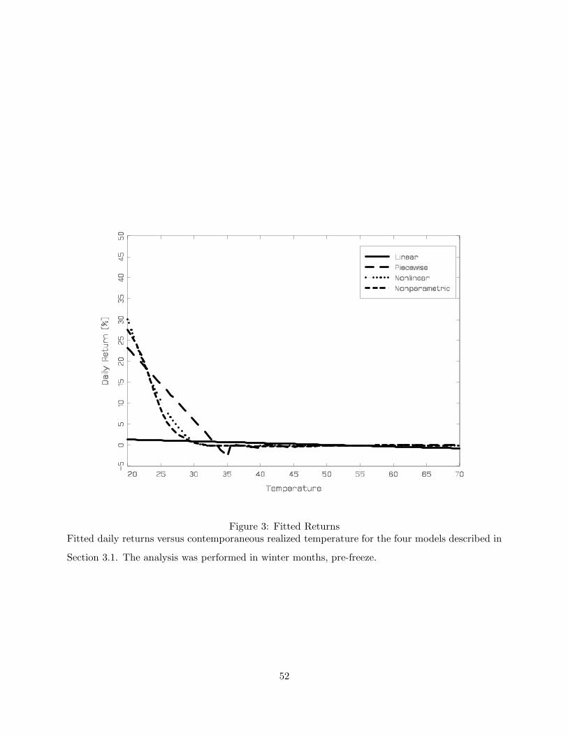
Figure 3: Fitted ReturnsFitted daily returns versus contemporaneous realized temperature for the four models described in
Section 3.1. The analysis was performed in winter months, pre-freeze.
52