Embed Size (px)
Citation preview
NBER WORKING PAPER SERIES
DEMOCRACY AND GROWTH
Robert I. Barro
Working Paper No. 4909
NATIONALBUREAU OF ECONOMIC RESEARCH1050 Massachusetts Avenue
Cambridge, MA 02138October 1994
I am grateful to Jong-Wha Lee and Jorthn Rappaport for help with the underlying data. Thisresearch has been supported in part by the National Science Foundation. This paper is part ofNBER's research program in Growth. Any opinions expressed are those of the author and notthose of the National Bureau of Economic Research.
© 1994 by Robert J. Barro. All rights reserved. Short sections of text, not to exceed twoparagraphs, may be quoted without explicit permission provided that full credit, including ©notice, is given to the source.

NBER Working Paper #4909October 1994
DEMOCRACY AND GROWTH
ABSTRACT
Growth and democracy (subjective indexes of political freedom) areanalyzed for a panel
of about 100 countries from 1960 to 1990. The favorable effects on growth include maintenance
of the rule of law, free markets, small government consumption, andhigh human capital. Once
these kinds of variables and the initial level of real per-capita GDPare held constant, the overall
effect of democracy on growth is weakly negative. There is a suggestion of a nonlinear
relationship in which democracy enhances growth at low levels of political freedom but depresses
growth when a moderate level of freedom has already been attained. Improvements in the
standard of living - measured by GDP, life expectancy, and education - substantially raise the
probability that political freedoms will grow. These results allow for predictions about which
countries will become more or less democratic in the future.
Robert J. BarroBank of EnglandMonetary Analysis, Room 326Threadneedle StreetLondon EC2 R8AHUNITED KINGDOMand NBER
Economic freedoms, in the form of free markets and small governments that focus
on the maintenance of property rights, are often thought to encourage economic growth.
This view receives support from the present study, which uses data from many countries
since 1960. The results confirm the importance of economic freedom and provide some
quantification of the linkages among growth rates, market distortions, the rule of law,
and other variables.
The connection between political and economic freedom is more controversial.
Some observers, such as Friedman (1962), believe that the two freedoms are mutually
reinforcing. In this view, an expansion of political rights—more "democracy"—fosters
economic rights and tends thereby to stimulate growth. But the growth retarding
features of democracy have also been stressed. These features involve the tendency to
enact rich—to-—poor redistributions of income (including land reforms) in systems of
majority voting and the enhanced role of interest groups in systems with representative
legislatures.
Authoritarian regimes may partially avoid these drawbacks of democracy.
Moreover, nothing in principle prevents nondemocratic governments from maintaining
economic freedoms and private property. A dictator does not have to engage in central
planning. Examples of autocracies that have expanded economic freedoms include the
Pinochet government in Chile, the Fujimori administration in Peru, the Shah's
government in Iran, and several previous and current regimes in East Asia.
Furthermore, as stressed by Schwarz (1992), most OECD countries began their modern
economic development in systems with limited political rights and became full—fledged
representative democracies only much later.
The effects of autocracy on growth are adverse, however, if a dictator uses his
power to steal the nation's wealth and to carry out nonproductiveinvestments. Many
governments in Africa, some in Latin America, some in the formerly planned economies
of eastern Europe, and the Marcos administration in the Philippines seem to fit this
model. Thus, history suggests that dictators come in two types, one whose personal
objectives often conflict with growth promotion and another whose interests dictate a
preoccupation with economic development. The theory that determines which kind of
dictatorship will prevail is presently missing.
Democratic institutions provide a check on governmental power and thereby limit
the potential of public officials to amass personal wealth and to carry out unpopular
policies. Since at least some policies that stimulate growth will also be politically
popular, more political rights tend to be growth enhancing on this count. Thus, the net
effect of democracy on growth is theoretically inconclusive.
Another question concerns the impact of economic development on a country's
propensity to experience democracy. This issue requires a positive analysis of the choice
of political institutions, but theoretical models of this process are not well developed.
Nevertheless, a common view—6upported by many case studies—is that prosperity
tends to inspire democracy. The overall cross—country evidence considered in this study
strongly supports this view; specifically, an increase in the standard of living tends to
generate a gradual rise in democracy. In contrast, democracies that arise without prior
economic development—sometimes because they are imposed from outside—tend not
to last.
Framework of the Empirical Analysis
The framework for the growth analysis is an extension of the neoclassical growth
model to include governmental functions and other elements.' The long-run or steady-
'The theory comes from Ramsey (1928), Solow (1956), Swan (1956), Cass (1965), andKoopmans (1965). For an exposition, see Barro and Sala—i—Martin (1994, Chs. 1 and 2).Previous empirical applications of the model include Barro (1991), Mankiw, Romer, andWell (1992), and Barro and Sala—i—Martin (1994, Ch. 12).
2
state level of per-capita output depends in this model on an array of choice and
environmental variables.2 The private sector's choices include the fertility andsaving
rates, each of which depends on preferences and costs. The government's choices involve
spending in various categories, tax rates, the extent of distortions of markets and
business decisions, maintenance of the rule of law and property rights, and the degree of
political freedom. Also relevant is the terms of trade, typically given to an individual
country by international conditions.
For a given initial level of per-capita output, an increase in the steady-state level
of per-capita output raises the per-capita growth rate over a transition interval. For
example, if the government improves the climate for business activity—say by reducing
the burdens from regulation, corruption, and taxation, or by enhancing property
rights—the growth rate increases for awhile. Similar effects arise if people decide to
have fewer children or (in a closed economy) to save a larger fraction of their incomes.
In all of these cases, an increase in the long-run level of per-capita output translates into
a transitional increase in the economy's growth rate. Moreover, because the transitions
tend to be lengthy, the growth effects persist for a long time.
For given values of the choice and environmental variables, a higher starting value
of per-capita output leads to a lower per-capita growth rate. This relation reflects
primarily the presence of diminishing returns to capital in the neoclassical model. As an
economy prospers, the return on investment declines, and the growth rate tends
accordingly to decrease. This effect may be modified by endogenous responses of the
saving rate, fertility, work effort, and migration. However, if diminishing returns apply,
then the force toward lower growth rates tends eventually to dominate.
2With exogenous, labor-augmenting technological progress, the level of output per workergrows in the long run, but the level of output per effective worker approaches a constant.
3
The inverse relation between the growth rate and level of per-capita output leads
to a well-known convergence property: poor economies tend to grow faster per capita
than rich ones and tend thereby to catch up to the rich ones. The discussion already
implies that this convergence force applies in the neoclassical model only in a conditional
sense. For given values of the choice and environmental variables, a lower starting
value of per-capita output tends to generate a higher growth rate. But a poor country
that has a low steady-state level of per-capita output—because, for example, it has
political institutions that are inhospitable to investment—need not grow faster than a
rich country. Since countries are likely to be poor or rich precisely because the
underlying determinants of their steady states are unfavorable or favorable, the model
does not predict any clear pattern of simple correlation between growth rates and
starting positions.
The diffusion of technology provides another force toward convergence. Since
imitation is usually cheaper than innovation, follower countries have an advantage here.
However, as the stock of adaptable but uncopied ideas decreases, this advantage
declines. The growth rates of follower economies tend accordingly to decrease with the
level of per-capita output much as in the neoclassical growth model with diminishing
returns to investment. The convergence predicted by technological diffusion is also
conditional on government policies and other elements that influence the returns from
introducing modern techniques to a follower economy. For example, a backward
country that does not respect property rights and has little infrastructure services will
not import much modern technology and will not grow rapidly.
The capital stock accumulated in the neoclassical model can be broadened to
include human capital (in the forms of education, experience, and health), as well as
physical capital and natural resources. (See Lucas [1988), Rebelo [1991], Caballe and
Santos [1993], and Barro and Sala—i—Martin [1994, Ch. 5J.) The economy tends toward
4
target ratios for the various kinds of capital, but these ratios may depart from their
target values in an initial state. The extent of these departures generally affects the rate
at which initial per-capita output approaches its steady-state value. For example, a
country that starts with a high ratio of human to physical capital (perhaps because of a
war that destroyed mainly physical capital) tends to grow rapidly because physical
capital is more amenable than human capital to rapid expansion. A supporting force is
that the adaptation of foreign technologies is facilitated by a large endowment of human
capital (see Nelson and Phelps [1966] and Benhabib and Spiegel [1993]). This element
implies an interaction effect whereby a country's growth rate is more sensitive
(inversely) to its starting level of per-capita output the greater is its initial stock of
human capital.
Empirical Findings on Growth across Countries
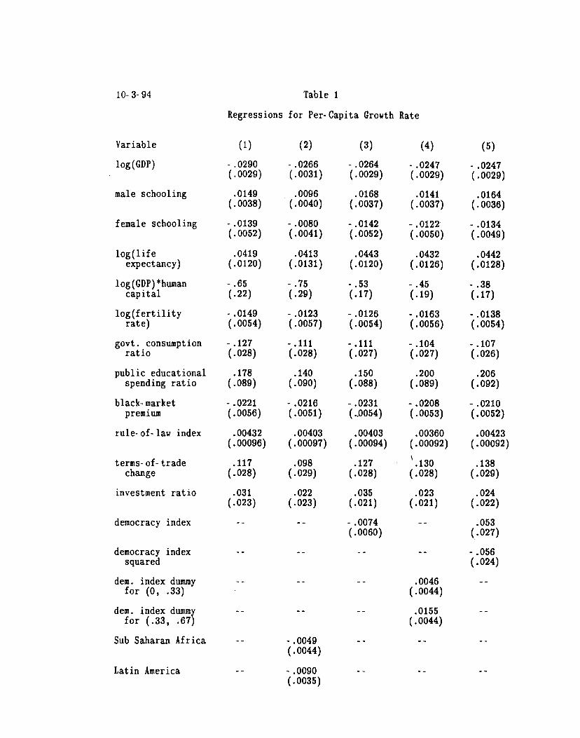
Table 1 shows the results from regressions that use the framework of the previous
section. See Table Al in the appendix for means and standard deviations of the
variables that appear in the analysis. The regressions apply to a panel of roughly 100
countries o1served from 1960 to 1990. The dependent variables are the growth rates of
real per-cajita GDP over three periods: 1965—75, 1975—85, and 1985—90. (The first
period begiis in 1965, rather than 1960, so that the 1960 value of the level of real per-
capita GDI can be used as an instrument; see below.) Henceforth, the term GDP will
be used as a shorthand to refer to real per-capita GDP.
3Most of the GDP figures are from version 5.5 of the Suinmers-Heston data set (seeSummers arid Heston [1991, 1993] for general descriptions). These values adjust forestimated differences in purchasing power across countries. World Bank figures on realGDP growth rates (based on domestic accounts only) are used for 1985—90 when theSummers-Heston figures are unavailable.
5
6
The estimation uses an instrumental-variable technique, where some of the
instruments are earlier values of the regressors.4 This approach may be satisfactory
because the residuals from the growth-rate equations for the various periods exhibit
little correlation. In any event, the regressions describe the relation between growth
rates and prior values of the explanatory variables.
The regression shown in column (1) includes explanatory variables that can be
interpreted as initial values of state variables or as choice and environmental variables.
The state variables include measures of human capital in the form of schooling and
health and the initial level of GDP. This GDP level reflects the endowments of physical
capital and natural resources (and also depends on effort and the unobserved level of
technology). The choice and environmental variables are the fertility rate, government
spending for consumption and education,5 the black-market premium on foreign
exchange, an index of the maintenance of the rule of law, the ratio of gross investment
to GDP, and the change in the terms of trade. A later analysis adds an index of
democracy.
Initial Level of GDP
For given values of the other explanatory variables, the neoclassical model predicts
a negative coefficient on initial GDP, which enters in the regression in logarithmic form.
4Countries are equally weighted in the regressions, but the estimation allows for differenterror variances for each period and for correlation of the errors across the periods. Theresults are virtually identical, however, if the error terms from the different periods aretreated as independent. See the notes to Table 1 for additional information.5Data problems prevent consideration of marginal tax rates and some other components ofovernment spending, such as transfers and infrasructure services. See Easterly and Rebelo(1993) for a discussion of these data. The ratio of defense spending to GDP turned out tobe insignflcant in the growth regressions.8The variable log(GDP) in Table 1 refers to 1965 in the first period 1975 in the secondperiod, and 1985 in the third period. Five-year earlier values of logGDP) are used asinstruments. The use of thes instruments lessens the estimation problems associated withtemporary measurement error in GDP.
7
The coefficient on the log of initial GDP has the interpretation of a conditional
rate of convergence, if the other explanatory variables are held constant, then the
economy tends to approach its long-run position at the rate indicated by the magnitude
of the coefficient. The estimated coefficient of —.0290 (s.e. = .0029) is highly significant.
This estimate implies a conditional rate of convergence of 2.9% per year.7
Initial Level of Human Capital
Initial human capital appears in four variables in the regressions: male and female
average years of attainment in secondary and higher schools for the adult population at
the start of each period, the log of life expectancy at birth at the start of each period,
and an interaction between the log of initial GDP and an overall human—capital
variable. Overall human capital is the sum of the levels of male and female school
attainment and the log of life expectancy, where each variable is multiplied by its
coefficient in the regression.8
The column (1) regression indicates a significantly positive effect on growth from
initial human capital in the form of health; the coefficient on the log of life expectancy is
.042 (.012). The results on education show the puzzling pattern des&ibed in Barro and
Lee (1994) in which the estimated coefficient on male attainment is significantly
positive, .015 (.004), whereas than on female attainment is significantly negative, —.014
(.005). If life expectancy is included in the regressions, as in Table 1, then it seems to
proxy for the level of human capital; the level of educational attainment then has no
This result is only approximate because the growth rate is observed as an average over tenor five years, rather than at a point in time. The implied instantaneous rate of
- convergence is slightly higher than the value indicated by the coefficient. See Barro andSala—i—Martin (1992) for a discussion.
The interaction term measures log(GDP) and human capital as deviations from samplemeans. This procedure makes it easier to interpret the regression coefficients on log(GDP),male and female schooling, and log of life expectancy.
8
additional explanatory power for growth. An additional positive effect on growth
emerges, however) when male attainment is high relative to female attainment. A
possible interpretation is that the gap between male and female schooling is an indicator
of an economy's backwardness and that greater backwardness induces a higher growth
rate through the familiar convergence mechanism.
The interaction term between initial GDP and human capital is significantly
negative, —.65 (.22), in column (1) of the table. This result indicates that a country
with more overall human capital tends to converge faster toward its long—run position.
The estimated coefficient on the interaction variable turns out, however, to be
dominated by a small number of outlying observations and is accordingly sensitive to
minor changes in specification. Therefore, this estimated effect may not be reliable.
Educational Spending
A likely difficulty with the educational variables is that they measure years of
attainment but do not adjust for school quality. The construction of a broad data set on
measures of quality—including school days per year, estimated salaries of teachers in
relation to country wage rates, teacher—pupil ratios, and the frequency of school
dropouts and repeaters—is ongoing. The ratio of public educational spending to GD?,
included in the regressions in Table 1, is intended as an imperfect proxy for school
quality. The estimated coefficient of this variable, .18 (.09), is positive and marginally
significant.
Fertility Rate
If the population is growing, then a portion of the economy's investment is used to
provide capital for new workers, rather than to raise capital per worker. For this reason,
a higher rate of population growth has a negative effect on the steady-state level of

output per effective worker in the neodassical growth model. Another, reinforcing,
effect is that a higher fertility rate means that increased resources are devoted to
childrearing, rather than to production of goods (see Becker and Barro [1988]). The
regression in column (1) shows a significantly negative coefficient, —.015 (.005), on the
log of the total fertility rate.
Fertility decisions are surely endogenous; previous research has shown that fertility
typically declines with measures of prosperIty, especially female education (see Schultz
[1989], Behrman [1990], and Barro and Lee [1994]). The estimated coefficient of the
fertility rate in the regression of column (1) can be interpreted as the response of growth
to higher fertility, for given schooling, life expectancy, GDP, and so on. Since the
average of the fertility rate over the preceding five years is used as an instrument, the
coefficient likely reflects the impact of fertility on growth, rather than vice versa. (In
any event, the reverse effect would involve the level of GD?, rather than its growth
rate.) Thus, although population growth cannot be described as the most important
element in economic progress, the results do suggest that an exogenous drop in birth
rates would raise the growth rate of per-capita output.
Government Consumption
The regression in column (1) also shows a significantly negative effect on growth
from the ratio of government consumption (measured exclusive of spending on education
and defense) to GD?. The estimated coefficient is —.13 (.03). (The period-average of
the ratio enters into the regression, and the average of the ratio over the previous five
years is used as an instrument.) The particular measure of government spending is
intended to approximate the outlays that do not enhance productivity. Hence, the
conclusion is that a greater volume of nonproductive government spending—and the
9

10
associated taxation—reduce the growth rate for a given starting value of GDP. In this
sense, big government is bad for growth.
Measures of Market Distortions: The Black—Maiket Premium and the Rule-of-Law
Index
The black-market premium on foreign exchange is a widely available and
apparently accurate measure of a particular price distortion (the gap between the official
exchange rate and the rate available to nonfavored market participants). The premium
likely serves as a proxy for governmental distortions of markets more generally. One
difficulty with the variable is the likelihood of reverse causation; economic difficulties
may pressure governments into exchange controls and other policies that lead to high
black-market premia. This problem is mitigated by the use of an average of the
premium over the previous five years as an instrument. (The period-average of the
premium appears in the regressions.) The estimated coefficient, —.022 (.006), is
significantly negative, thereby suggesting that distortions of markets are adverse for
economic growth.
Knack and Keefer (1994) discuss a variety of subjective country indexes prepared
for fee-paying international investors by International Country Risk Guide. The
measures gauge the maintenance of the rule of law, political corruption, risk of
repudiation of contracts, and so on. The rule-of-law index (measured on a 0 to 6 scale,
with 6 the most favorable) appeared, a priori, to be the most relevant of these indicators
for gauging the attractiveness of a country's investment climate. Thus, the rule-of-law
variable is entered into the column (1) regression and has a significantly positive
coefficient, .0043 (.0010). (The other measures of investment risk are insignificant in the
growth regression if the rule-of-law index is also included.) The desired interpretation is
that greater maintenance of the rule of law is favorable to growth.
11
A major problem is that the figures on the rule of law and the other subjective
indicators are available from International Country Risk Guide starting only in the early
1980s. The results shown in Table 1 use a single observation—that for the earliest year
available in the 1980s—for each country. The equations for growth in 1965—75 and
1975—85 therefore use as an explanatory variable a later or contemporaneous value of
the rule-of-law index. The justification for this procedure is that a country's
institutional structure that governs the enforcement of laws and contracts tends to
persist over long periods. Therefore, the value for the early 1980s is typically a good
proxy for the values that prevailed earlier and later. The possibility of reverse
causation—low growth stimulating the deterioration of law enforcement (or influencing
the perceptions of International Country Risk Guide)—is, however, especially serious
for the 1965—75 regression.
Knack and Keefer (1994) provide information from another consulting service for
the early 1970s on the quality of the bureaucracy, the degree of contract enforcement,
and some other variables. The figures apply, however, to a much smaller number of
countries. These data can be used as instruments for the rule-ofaw index for the
1975—85 equation. The system then loses the 82 observations for 1965—75, has 44
observations (instead of 89) for 1975—85, and retains 84 observations for 1985—90 (for
which the rule—of—law variable enters as an instrument). In this case, the estimated
coefficient on the rule-of-law variable is .0031 (.0019), now only marginally significant,
but not significantly different from the value shown in column (1) of Table 1. Since the
point estimate changes little when these instruments are used, it is plausible that the
estimated coefficient in column (1) reflects mainly the effect of the rule of law on
growth, rather than vice versa.
The information appeared contemporaneously starting in the 1980s and could not thereforebe influenced by a country's subsequent experience, including its rate of economic growth.
Another issue is the use of the rule—of—law index as a cardinal variable. As
already mentioned, the index takes on the 7 possible integers from 0 to 6. Although the
values may be meaningful on an ordinal sca.le—that is, a higher number signifies more
respect for the rule of law—there is no guarantee that the variable has a cardinal
meaning. Thus, even if the relation between the growth rate and some cardinal measure
of the rule of law were linear, the relation with the ordinal index need not be linear.
Linearity can be checked by using dummy variables: specifically, one dummy
variable is defined to equal 1 for places in rule—of—-law categories 0, 1, and 2 and to
equal 0 otherwise; another dummy equals 1 for places in categories 3 and 4 and equals 0
otherwise. Places with values of 5 and 6 have both dummies set to 0. The mean value
of the rule-of-law index over the relevant sample of countries is 1.2 for the first group
(only Guyana and Haiti have index values of 0), 3.5 for the second group, and 5.8 for the
third group.
The system from column (1) of Table 1 was reestirnated with the two dummy
variables replacing the rule—of--law index. The estimated coefficient on the first dummy
is —.02 1 (.004) and that on the second is —.016 (.004). (The other results are similar to
those shown in column [1].) Thus, the countries in the lowest groups for the
rule—of—law variable had the worst growth performance, those ranked in the middle
came second, and those ranked highest did the best. If the relation were linear, then the
coefficient on the first dummy would be roughly twice that on the second dummy (based
on the means of the rule—of—law index within each group). A test of this restriction has
a p—value of .05. Thus, although strict linearity would be barely rejected at the 5%
level, the hypothesis is not greatly at odds with the data. The remainder of the analysis
therefore retains the form in which the rule—of—law index enters directly as a regressor.
12
Investment Ratio
In the neoclassical growth model for a closed economy, the saving rate is
exogenous and equal to the ratio of investment to output. A higher saving rate raises
the steady-state level of output per effective wcrker and thereby raises the growth rate
for a given starting value of GDP. Some empirical studies of cross-country growth have
also reported an important positive role for the investment ratio; see, for example,
DeLong and Summers (1991) and Mankiw, Romer, and Weil (1992).
Reverse causation is, however, likely to be important here. A positive coefficient
on the contemporaneous investment ratio in a growth regression may reflect the positive
relation between growth opportunities and investment, rather than the positive effect of
an exogenously higher investment ratio on the growth rate. This reverse effect is
especially likely to apply for open economies. Even if cross-country differences in saving
ratios are exogenous with respect to growth, the decision to invest domestically, rather
than abroad, would reflect the domestic prospects for returns on investment, which
would relate to the domestic opportunities for growth.
The regression in column (1) of Table 1 contains the period-average investment
ratio as an explanatory variable but uses the average of the investment ratio over the
preceding five years as an instrument. The estimated coefficient, .031 (.023), is positive,
but not statistically significant. In contrast, the estimated coefficient is more than twice
as high and statistically significant if the period-average investment ratio is induded as
an instrument. These findings suggest that much of the positive estimated effect of the
investment ratio on growth in typical cross-country regressions reflects the reverse
relation between growth prospects and investment. The direct effect of exogenously
higher investment on. growth—which is perhaps shown by the estimated coefficient in
column (1)—is much smaller than usually thought. (Blamstrom,Lipsey, and Zejan
[1993] reach similar conclusions in their study of investment and growth.)
13
14
Terms of Trade
Changes in the terms of trade have often been discussed as an important influence
on developing countries; which typically specialize their exports in a few primary
products. The effect of a change in the terms of trade—measu.red as the ratio of export
to import prices—on GDP is, however, not mechanical. If the physical quantities of
goods produced domestically do not change, then an improvement in the terms of trade
raises real domestic income and probably consumption, but would not affect real GDP.
Movements in real GDP result only if the shift in the terms of trade stimulates a change
in domestic employment and output. For example, an oil-importing country might react
to an increase in the relative price of oil by cutting back on its employment and
production.
The result in column (1) of Table 1 shows a significantly positive coefficient on the
growth rate of the terms of trade: .12 (.03). (The change in the terms of trade is
regarded as exogenous to an individual country's growth rate and is therefore included
as an instrument.) Thus, an improvement in the terms of trade apparently does
stimulate an expansion of domestic output.1°
Dnmmies for Africa, Lathi America, and East Asia
Previous research, such as Barro (1991), indicates that countries in Sub Saharan
Africa and Latin America grow at significantly lower rates even after holding fixed a set
of explanatory variables in a regression. This kind of analysis suffers from a selection
bias in that the choice of which dummy variables to consider for geographical areas is
10Barro and Sala—i—Martin (1994, Ch. 12) consider some other regressors. One variableincluded in that framework and in Alesina and Perotti (1993) is political instability,measured by the frequencies of revolutions and other disruptions. The political—instabilityvariables are, however, not significantly related to growth when the rule—of--law index isalso included in the reressions. King and Levine (1993) explore the effects of financialdevelopment, and Cukierman (1992) assesses the influences from inflation and central-bankindependence.
15
dictated by the prior observation that some places have especially low or high growth
rates. Nevertheless, the confidence in the growth-rate specification would be enhanced if
the included regressors already explained why the typical country in Sub Saharan Africa
and Latin America grew at below-average rates.
The regression in column (2) of Table 1 adds dummy variables for Sub Saharan
Africa, Latin America, and East Asia (a high-growth area). The result is that only the
estimated coefficient for Latin America, —.009 (.004), is individually statistically
significant at usual critical levels. The coefficient for Sub Saharan Africa is negative,
—.005 (.004), but insignificant, whereas that for East Asia is positive, .004 (.004), but
also insignificant. A joint test that the coefficients of all three dummy variables are zero
has a p—value of .031. Thus, although there is still an indication of an omitted adverse
effect on growth in Latin America, the present specification accounts well for the high
average growth in East Asia and is much better than previous specifications in
explaining the low average growth in Sub Saharan Africa.
Democracy
The measure of democracy is the indicator of political rights compiled by Gastil
and his followers (1982—83 and subsequent issues) from 1972 to 1993. A related variable
from Bolien (1990) is used for 1960 and 1965." The Gastil concept of political rights is
indicated by his basic definition: ttPolitical rights are rights to participate meaningfully
in the political process. In a democracy this means the right of all adults to vote and
compete for public office, and for elected representatives to have a decisive vote on
"The discussion in Bollen (1990) suggests that his measures are comparable to Gastil's. It isdifficult to check comparability directly because the two series do not overlap in time.Moreover, many countries—especially those in Africa—clearly experienced major declinesin the extent of democracy from the 1960s to the 1970s. Thus, no direct inference aboutcomparability can be made from the higher average of Bollen's figures for the 1960s thanfor Gastil's numbers for the 1970s.
16
public policies." (Gastil, 1986—87 edition, p. 7.) In addition to the basic definition, the
classification scheme counts as less democratic countries that have dominant political
parties in which minority groups have little influence on policy.
Operationally, the concept of political rights is applied on a subjective basis to
classify countries annually on a scale from 1 to 7, where 1 is the highest level of political
rights. The classification is made by Gastil and his associates based on an array of
published and unpublished information about each country. Unlike the rule—of-—law
index discussed before, the subjective ranking is not made directly by local observers.
The original ranking from ito 7 has been converted here to a scale from 0 to 1,
where 0 corresponds to the fewest political rights (Gastil's rank 7) and 1 to the most
political rights (Gastil's rank 1). The scale from 0 to 1 corresponds to the system used
by Bollen.
Figure 1 shows the time path of the unweighted average of the democracy index
for 1960, 1965, and 1972—93. The number of countries covered rises from 98 in 1960 to
109 in 1965 and 134 from 1972 to 1993. The figure shows that the mean of the
democracy index peaked at .66 in 1960, fell to a low point of .44 in 1975, and rose
subsequently to .57 in 1992—93.
Figures 2 and 3 demonstrate that the main source of the decline in democracy after
1960 is the experience in Sub Saharan Africa. Figure 2 indicates that many of the
African countries began with democratic institutions when they became independent in
the early 1960s, but most had evolved into nondemocratic states by the early 1970s.
(See Bollen [1990] for further discussion.) For countries outside of Sub Saharan Africa,
Figure 3 shows that the average of the democracy index fell from .69 in 1960 (72
countries) to .54 in 1975 (91 countries) and then returned to .68 in 1990—92 (but fell to
.67 in 1993).
17
The discussion in the introduction indicated that the net effect of more political
freedom on growth is theoretically ambiguous. Column (3) of Table 1 shows the
regression results when the democracy index is included as an explanatory variable in
the growth equations. The estimated coefficient, —.0074 (.0060), is negative, but not
statistically different from 0 at conventional critical levels. The point estimate implies
that a one—standard—deviation increase in democracy (by 0.3 in the indicator, see Table
Al) reduces the growth rate by .002 per year. Thus, the results are consistent with a
moderate adverse influence of democracy on growth.
Some previous studies, such as Kormendi and Meguire (1985) and Scully (1988),
report favorable effects of political freedom on growth. It is possible to replicate these
ki$s of results within the present framework by eliminating some of the other
independent variables from the regressions. For example, if the variables for the rule of
law, schooling, life expectancy, and fertility are omitted, then the estimated coefficient
of democracy becomes significantly positive, .0141 (.0067). A reasonable interpretation
is that democracy looks favorable for growth in this specification only because
democracy is positively correlated with some omitted country characteristics that are
themselves growth enhancing. Once these other variables are held constant, the
marginal contribution of democracy to growth becomes moderately negative.'2
Democracy may also influence growth indirectly by affecting some of the
explanatory variables that are held constant in the regressions. For example, more
political rights might stimulate female education (by promoting equality among the
sexes), which in turn reduces fertility and thereby promotes growth. However, if
fertility and female schooling are omitted from the growth equations (but male
12A possible argument is that the index of political freedom has so much measurement errorthat true democracy is more correlated with some of the other variables than with thedemocracy variable. It is undear, however, that the subjective measure of political rightsis less accurate than some of the other variables, especially for the poorer countries.
schooling, life expectancy and the rule-of4aw index are retained), then the estimated
coefficient on the democracy variable is 8tiU negative, —.009 (.006). Hence, the channel
through female schooling and fertility is not sufficient for democracy to show up as a
positive influence dn growth.
Another possibility is that democracy encourages maintenance of the rule of law.
Tests of this hypothesis are hampered by the limited availability of time-series
information on the rule-of-law concept. For a sample of 47 countries, it is possible to
consider the dynamic relation between the rule-of-law index, which applies to the early
1980s, and the previously discussed measures of bureaucratic delay and contract
enforcement, which apply to the early 1970s. A regression for the rule-of-law variable
that includes these two measures, along with log(GDP) for 1975, log(life expectancy) for
1970—74, and democracy for 1975 has a coefficient of —.61 (.71) on democracy. Thus,
this limited evidence suggests that democracy does not promote the maintenance of the
rule of law.
The analysis thus far has considered only linear relations between growth and
democracy. The relation may be nonlinear because the democracy index—based on
Gastil's (1982—83) seven subjective categories—has only an ordinal meaning and also
because the true relation between growth and democracy could be nonlinear. For
example, in the worst dictatorships, an increase in political rights might be growth
enhancing because of the benefit from limitations on governmental power. But in places
that have already achieved a moderate amount of democracy, a further increase in
political rights might impair growth because of the intensified concern with income
redistribution.
Column (4) of Table 1 shows the results when the democracy index is replaced by
two dummy variables. The first dummy equals 1 if the democracy index is between 0
and .33 and equals 0 otherwise, and the second dummy equals 1 if the index is between
18
.33 and .67 and equals 0 otherwise. If the democracy index exceeds .67, then both
dummies equal 0. The estimated coefficients are .005 (.004) for the first dummy and
.016 (.004) for the second. The p—value for the joint significance of the two dummy
variables is .00 1. (The hypothesis of linearity—requiring that the coefficient of the first
dummy be roughly double that of the first—rnis strongly rejected.)
The results indicate that the middle level of democracy is most favorable to
growth, the lowest level comes second, and the highest level comes third. The strongest
part of this finding is the superiority of the middle level over the other two; the lowest
arid highest groups do not have significantly different growth rates (given the values of
the other independent variables).
Similar conclusions emerge if the democracy index is entered directly in a
quadratic form. Column (5) of Table 1 shows that the estimated coefficient on the
linear term is positive, .053 (.027), whereas that on the squared term is negative, —.056
(.024). The p—value for joint significance of the two terms is .02. In this form, the
results suggest that, at low levels of democracy, more political freedom enhances growth.
The growth rate reaches a peak at a middle level of democracy—the point estimate is
.47—and then diminishes if democracy continues to rise.
Figure 4 shows the nature of the partial relation between the growth rate and the
level of democracy. The vertical axis plots the part of the growth rate that is
unexplained by the independent variables other than the democracy index and its square
(from the regression in column [5] of Table 1). The scatter diagram shows how this
"partial residual" relates to the democracy index. An inverse u—shape can be discerned
in the plot, with many of the low and high democracy places exhibiting negative
residuals. Only a few of the countries with middle levels of democracy (Argentina and
Peru) have negative residuals. However, the overall relation is far from perfect; for
example, a number of countries with little democracy have large positive residuals.
19
20
Also, the places with middle levels of democracy seem to avoid low growth rates but not
to have especially high growth rates. Thus, at this point, there is only the suggestion of
a nonlinear relation in which more democracy raises growth when political freedoms are
weak but depresses growth when a moderate amount of freedom is already established.
Sources of Growth
Table 2 uses groups of slow— and fast—growing countries to illustrate how the
fitted growth rates break down into contributions from the individual explanatory
variables. The countries considered fall into the lowest or highest quintiles of growth
rates from 1965 to 1990. Group I in the table has 15 slow—growing Sub Saharan African
countries, group II has 6 slow—growing Latin American countries, group III has 9
fast—growing East Asian countries, and group IV has 6 fast—growing European
countries. The table can be used to see how the model "explains" or fails to explain the
sharp differences in growth performance among the four groups of countries.
The fitted growth rates in Table 2 come from a regression that excludes the
democracy variable; that is, the one shown in column (1) of Table 1. These fitted values
are expressed relative to the sample mean in each period (see Table Al). For a typical
poor country, the contribution to fitted growth from log(GDP) is positive, but this
effect is offset by negative contributions from human capital and fertility (because GDP
is strongly positively correlated with human capital and strongly negatively correlated
with fertility). For this reason, it is helpful to think of a net convergence effect, which
combines the contributions from log(GDP) with those from human capital and fertility.
The contribution to fitted growth from this net convergence effect is shown along with
the individual elements in Table 2.
The table shows that the net convergence effects for the African and European
countries are each close to zero in the 1965—?5 period. For Africa, the positive effect
from low GDP is offset by low values of human capitaland high values of fertility,
whereas in Europe, the negative effect from high GDP is offset by high values of human
capital and low values of fertility. In contrast to these experiences, the East Asian
countries have a substantial positive contribution from net convergence, .019, because
human capital (especially male schooling) starts out high relative to GDP.
For the Latin American countries, a noteworthy result is the adverse contribution
from high market distortions, especially toward the end of the sample. For 1985—90, the
contributions to growth are —.013 from the black—market premium and —.008 from the
nile-of--law index (which does not vary over time). The African countries also suffer
from large distortions, whereas the East Asian and European countries benefit from
small distortions. High government consumption is another negative contributor for
Africa. The terms—of—trade change, although often mentioned as a key element in
Africa, is not a major element for any of the groups.
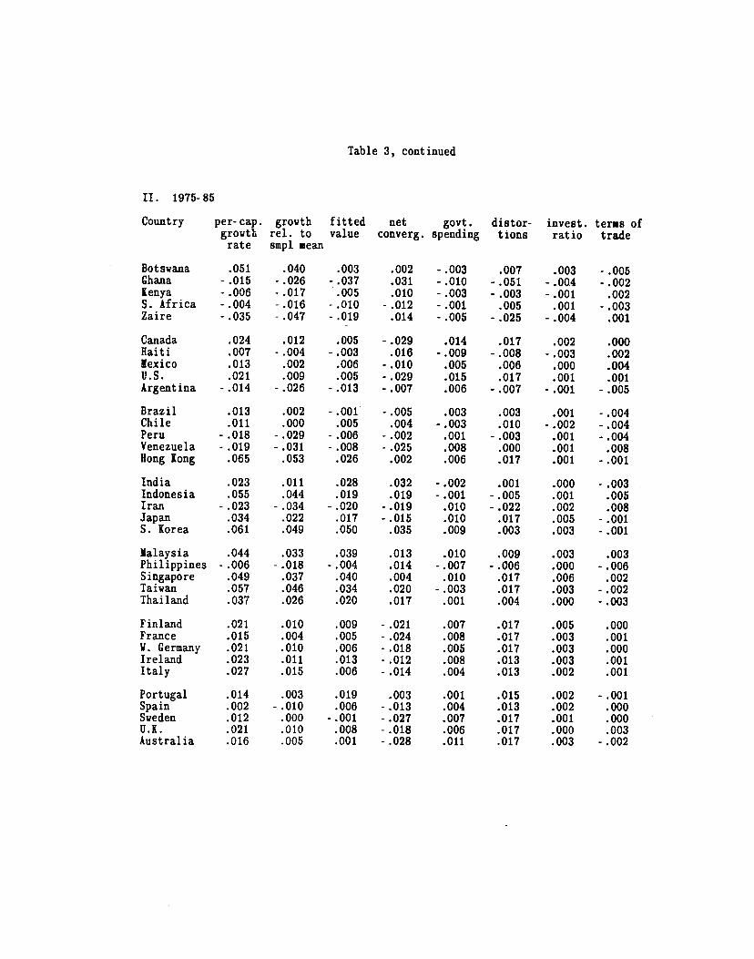
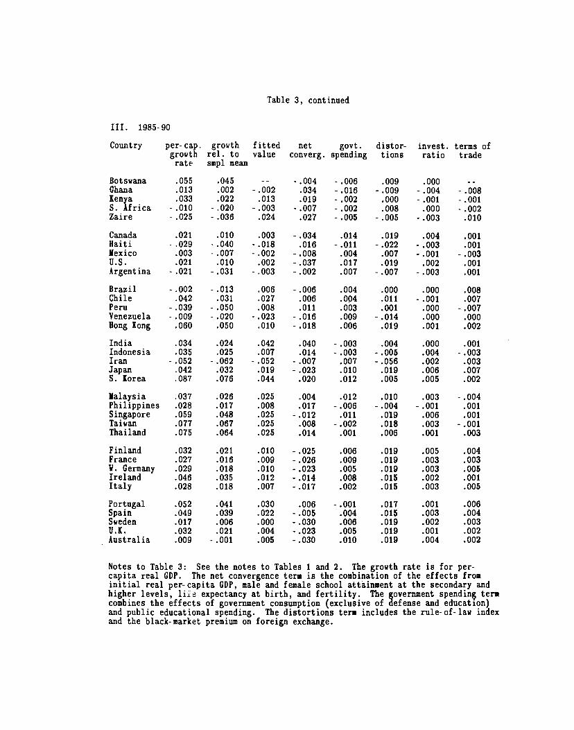
Table 3 uses the same approach to illustrate sources of growth by time period for
35 individual countries. l.a this case, the breakdown by components is less detailed,
consisting of the net convergence effect, the total influence of government consumption
and public education (a government spending effect), the combined impact from the
rule—of--law index and the black—market premium (an overall distortions effect), the
influence of the investment ratio, and the effect of the change in the terms of trade.
Effects of Economic Development on Democracy
Theories of how democracy expands or contracts seem to be missing. A look at the
data suggests, however, that countries at low levels of development typically do not
sustain democracy. For example, the political freedoms installed in most of the newly
independent African states in the early 1960s did not tend to last. Conversely,
nondemocratic places that experience substantial economic development have a
21
22
tendency to become more democratic. Examples include Chile, Korea, Taiwan, Spain,
and Portugal.
Table 4 contains regressions that test the hypothesis that prosperity stimulates the
development of democratic institutions. The dependent variables are the averages of the
democracy indexes over three periods of roughly a decade, 1965—74 (based on data for
1965 and 1972—74), 1975—84, and 1985—93. The explanatory variables are indicators of
the level of the standard of living; GDP, life expectancy at birth, and educational.
attainment. The schooling figures that turn out to be important here are the years of
attainment at the primary level for males and females.
The framework amounts to an error..correction model: the long-run target for
democracy depends on the standard of living, and democracy tends to rise or fall
depending on whether the target is above or below the current level of democracy.
Thus, column (1) of Table 4 indudes as a regressor the lagged value of democracy; 1960
in the 1965—74 equation, 1972 (1970 is unavailable) in the 1975—84 equation, and 1980
in the 1985—93 equation. The measures of standard of living refer, respectively, to 1965,
1975, and 1985.
The significantly positive coefficients on log(GDP) and log(life expectancy)
indicate that the target level of democracy is increasing in these indicators of the
standard of living.'3 Female school attainment is also significantly positive, whereas
male attainment is significantly negative. This finding is reminiscent of the results in
the growth regressions, where a larger gap between male and female attainment was
viewed as a signal of greater backwardness. In Table 4, a smaller excess of male over
female attainment signals less backwardness—that is, a more advanced society—and
thereby raises the target level of democracy.
'3HelliweU (1992, Table 1) finds that the Gastil measures of political rights and civil libertiesare positively related to levels of GDP and secondary—school enrollment ratios.

In column (1) of Table 4, the estimated coefficient on the lag of democracy, .46
(.04), is significantly positive, but also significantly less that one. This result indicates
that a country's level of democracy tends to move in a decade roughly half the way
toward the value associated with its standard of living.
In olumn (2), the process of adjustment is related to two lags of democracy.
(Because of lack of data before 1960, this system includes only two equations.) The
estimated coefficients on the lagged democracy variables, .36 (.05) and .13 (.05), are
each significantly positive. Thus, this pattern of adjustment depends not only on the
most recent value of democracy but also on the longer term history. The pattern still
implies that democracy adjusts gradually toward the values implied by the indicators of
the standard of living. The estimated coefficients on these indicator variables in column
(2) are similar to those in column (1).
The results from Table 4 can be used to forecast changes in the level of democracy
from the last value observed, 1993, into the future. These forecasts are based on 1990
values of GDP and life expectancy and on 1985 values of educational attainment (the
latest figures available). The projections can be viewed as applying roughly to the year
2000.
Table 5 displays the results for cases in which the forecasted change in democracy
has a magnitude of at least .14, which corresponds to a shift by 1 category in the Gastil
ranking. For the equation from column (2) of Table 4, 20 of 101 countries with all of
the necessary data are projected to increase democracy by at least .14, whereas 15 are
projected to decrease by at least .14.
The group with large projected increases in democracy, on the left side of Table 5,
includes some countries that have virtually no political freedom in 1993. Some of these
are among the world's poorest countries, such as Sudan and Haiti, for which the
projected level of democracy in 2000 is also not high. Sudan is forecasted to raise its
23
24
democracy from 0 in 1993 to .24 in 2000, and Haiti is also expected to go (perhaps with
the assistance of the United States) from 0 to .24. Some other countries that have
essentially no political freedom in 1993 are more well off economically and are therefore
forecasted to have greater increases in democracy; for example, the projected value in
2000 is .43 for Indonesia, .33 for Algeria, and .32 for Syria.
Expectations for large increases in democracy also apply to some reasonably
prosperous places in which the measured level of political freedom lags behind the
standard of living. Singapore is projected to increase its democracy index from .33 in
1993 to .61 in 2000, Mexico is expected to go from .50 to .72 (a change that has probably
already occurred with the 1994 elections), Fiji is anticipated to advance from .50 to .68,
and Taiwan is forecasted to rise from .50 to .64. Japan, which fell from 1.00 in 1992 to
.83 in 1993 because of the political corruption scandals, is projected to return to .97 by
2000. For Peru, where the democracy index declined from .83 in 1989 to .33 in 1993
(and in which economic freedoms were strengthened), the model projects an increase to
.51 in 2000.
South Africa is also included on the left side of the table, with a projected rise in
the democracy index from .33 in 1993 to .47 in 2000. However, the political changes in
South Africa in 1994 have probably overshot the mark, and the model would likely
forecast a substantial decline of political freedom in this country after 1994.
The examples of large expected decreases in democracy, shown on the right side of
Table 5, consist mainly of relatively poor countries with surprisingly high levels of
political freedom in 1993. Many of these cases are African countries in which the
political institutions recently became more democratic; Mali, Benin, Zambia, Central
African Republic, Niger, and Congo. The regression predicts that, as with the African
experience of the 1960s, democracy that gets well ahead of economic development will
not last. Three other African countries, The Gambia, Mauritius, and Botswana, have
maintained democratic institutions for some time, but the regression still predicts that
political freedoms will eventually diminish in these places. (A military coup in July
1994 has already reduced the Gambia's level of political freedom.)
For poor, but relatively democratic countries outside of Africa, the forecast for
large decreases in democracy applies to Bangladesh, Bolivia, Nepal, Pakistan, and
Papua New Guinea. Hungary, which has a higher standard of living, is projected to
decline from its fully democratic condition of 1.00 in 1993 to .81 in 2000.
Conduding observations
The interplay between democracy and economic development involves the effect of
political freedom on growth and the influence of the standard of living on the extent of
democracy. With respect to the determination of growth, the cross-country analysis
brings out favorable effects from maintenance of the rule of law, free markets, small
government consumption, and high human capital. Once these kinds of variables and
the initial level of GDP are held constant, the overall effect of democracy on growth is
wealdy negative. There is some indication of a nonlinear relation in which more
democracy enhances growth at low levels of political freedom but depresses growth when
a moderate level of political freedom has already been attained.
With respect to the effects of economic development on democracy, the analysis
shows that improvements in the standard of living—measured by a Country's real per-
capita GDP, life expectancy, and education—substantially raise the probability that
political institutions will become more democratic over time. Hence, political freedom
emerges as a sort of luxury good. Rich places consume more democracy because this
good is desirable for its own sake and even though the increased political freedom may
have a small adverse effect on growth. Basically, rich countries can afford the reduced
rate of economic progress.
25

The analysis has implications for the desirability of exporting democratic
institutions from the advanced western countries to developing nations. The first lesson
is that more democracy is not the key to economic growth, although it may have a weak
positive effect for countries that start with few political rights. The second message is
that political freedoms tend to erode over time if they are out of line with a country's
standard of living.
The more general conclusion is that the advanced western countries would
contribute more to the welfare of poor nations by exporting their economic systems,
notably property rights and free markets, rather than their political systems, which
typically developed after reasonable standards of living had been attained. If economic
freedom can be established in a poor country, then growth would be encouraged and the
country would tend eventually to become more democratic on its own. Thus, in the
long run, the propagation of western-style economic systems would also be the effective
way to expand democracy in the world.
26
References
Alesina, Alberto and Roberto Perotti (1993). "Income Distribution, Political
Instability, and Investment," National Bureau of Economic Research working
paper no. 4486, October.
Barro, Robert J. (1991). "Economic Growth in a Cross Section of Countries," Quarterly
Journal of Economics, 106, 2 (May), 407—433.
Barro, Robert J. and Jong—Wha Lee (1994). "Sources of Economic Growth," Carnegie—
Rochester Conference Series on Public Policy.
Barro, Robert J. and Xavier Sala—i—Martin (1992). "Convergence," Journal of Political
Economy, 100, 2 (April), 223—251.
Barro, Robert J. and Xavier Sala—i—Martin (1994). Economic Growth, New York,
McGraw Hill.
Becker, Gary S. and Robert J. Barro (1988). "A Reformulation of the Economic Theory
of Fertility," Quarterly Journal of Economics, 103, 1 (February), 1—25.
Behrman, Jere R. (1990). "Women's Schooling and Nonniarket Productivity: A Survey
and a Reappraisal," unpublished paper, University of Pennsylvania.
Benhabib, Jess and Mark M. Spiegel (1993). "The Role of Human Capital and Political
Instability in Economic Development," unpublished paper, New York University.
Blömstrorn, Magnus, Robert E. Lipsey, and Mario Zejan (1993). "Is Fixed Investment
the Key to Economic Growth?," National Bureau of Economic Research working
paper no. 4436, August.
Bollen, Kenneth A. (1990): "Political Democracy: Conceptual and Measurement
Traps," Studies in Comparative International Development, Spring, 7—24.
27
Caballe, Jordi and Manuel S. Santos (1993). "On Endogenous Growth with Physical
and Human Capital," Journal of Political Economy, 101, 6 (December),
1042—1067.
Cass, David (1965). "Optimum Growth in an Aggregative Model of Capital
Accumulation," Review of Economic Studies, 32 (July), 233—240.
Cukierrnan, Alex (1992). Central Bank Strategy, Credibility, and Independence,
Cambridge MA, MIT Press.
DeLong, J. Bradford and Lawrence H. Summers (1991). "Equipment Investment and
Economic Growth," Quarterly Jounwi of Economics, 106, 2 (May), 445—502.
Easterly, William and Sergio Rebelo (1993). "Fiscal Policy and Economic Growth: An
Empirical Investigation," Journal of Monetary Economics, 32 (December),
417—458.
Friedman, Milton (1962). Capitalism and Freedom, Chicago, University of Chicago
Press.
Gastil, Raymond D. and followers (1982—83 and other years). Freedom in the World,
Westport CT, Greenwood Press.
Helliwell, John (1992). "Empirical Linkages Between Democracy and Economic
Growth," unpublished paper, Harvard University, April.
King, Robert G. and Ross Levine (1993). "Finance, Entrepreneurship, and Growth:
Theory and Evidence," Joursial of Monetary Economics, 32 (December), 513—542.
Knack, Stephen and Philip Keefer (1994). "Institutions and Economic Performance:
Cross—Country Tests Using Alternative Institutional Measures," unpublished
paper, American University, February.
Koopmans, TjaLling C. (1965). "On the Concept of Optimal Economic Growth," in The
Econometric Approach to Development Planning, Amsterdam, North Holland.
28
Kormendi, Roger C. and Philip G. Meguire (1985). "Macroeconomic Determinants of
Growth11' Journal of Monetary Economics, 16, 141—163.
Lucas, Robert E., Jr. (1988). "On the Mechanics of Development Planning," Journal of
Monetary Economics, 22, 1 (July), 3—42.
Mankiw, N. Gregory, David Romer, and David N. Weil (1992). "A Contribution to the
Empirics of Economic Growth," Quarterly Journal of Economics, 107, 2 (May).
Nelson, Richard R. and Edmund S. Phelps (1966). "Investment in Humans,
Technological Diffusion, and Economic Growth," American Economic Review, 56,
2 (May), 69—75.
Ramsey, Frank (1928). "A Mathematical Theory of Saving," Economic Journal, 38
(December), 543—559.
Rebelo, Sergio (1991). "Long—Run Policy Analysis and Long—Run Growth," Journal of
Political Economy, 99, 3 (June), 500—521.
Schultz, T. Paul (1989). "Returns to Women's Education," PHRWD background
paper 89/001, The World Bank, Population, Health, and Nutrition Department,
Washington D.C.
Schwarz, Gerhard (1992). "Democracy and Market—Oriented Reform—A Love—Hate
Relationship?," Economic Education Bulletin, 32, 5 (May).
Scully, Gerald W. (1988). "The Institutional Framework and Economic Development,"
Journal of Political Economy, 96, 3 (June), 652—662.
Solow, Robert M. (1956). "A Contribution to the Theory of Economic Growth,"
Quarterly Journal of Economics, 70, 1 (February), 65—94.
Summers, Robert and Alan Heston (1991). "The Penn World Table (Mark 5): An
Expanded Set of International Comparisons, 1950—1988," Quarterly Journal of
Economics, 106, 2 (May), 327—368.
29
Summers; Robert and Alan Heston (1993). "Penn World Tables, Version 5.5," available
on diskette from the National Bureau of Economic Research, Cambridge MA.
Swan, Trevor W. (1965). "Economic Growth and Capital Accumulation," Economic
Record, 32 (November), 334—361.
30
10-3-94 Table 1
Regressions for Per-Capita Growth Rate
Variable (1) (2) (3) (4) (5)
log(GDP)- .0290 - .0266 - .0264 - .0247 - .0247(.0029) (.0031) (.0029) (.0029) (.0029)
male schooling .0149 .0096 .0168 .0141 .0164
(.0038) (.0040) (.0037) (.0037) (.0036)
female schooling - .0139 - .0080 - .0142 - .0122 - .0134(.0052) (.0041) (.0052) (.0050) (.0049)
log(life .0419 .0413 .0443 .0432 .0442
expectancy) (.0120) (.0131) (.0120) (.0126) (.0128)
log(GDP)*human- .65 - .75 - .53 - .45 - .38
capital (.22) (.29) (.17) (.19) (.17)
log(fertility- .0149 - .0123 - .0126 - .0163 - .0138
rate) (.0054) (.0057) (.0054) (.0056) (.0054)
govt. consumption - .127 - .111 - .111 - .104 - .107ratio (.028) (.028) (.027) (.027) (.026)
public educational .178 .140 .150 .200 .206spending ratio (.089) (.090) (.088) (.089) (.092)
black-market - .0221 - .0216 - .0231 - .0208 - .0210premium (.0056) (.0051) (.0054) (.0053) (.0052)
rule-of-law index .00432 .00403 .00403 .00360 .00423
(.00096) (.00097) (.00094) (.00092) (.00092)
terms-of-trade .117 .098 .127 '.130 .138
change (.028) (.029) (.028) (.028) (.029)
investment ratio .031 .022 .035 .023 .024
(.023) (.023) (.021) (.021) (.022)
democracy index - .0074 .053
(.0060) (.027)
democracy index - .056squared (.024)
dem. index dummy .0046
for (0, .33) (.0044)
dem. index dummy .0155
for (.33, .67) (.0044)
Sub Saharan Africa - .0049(.0044)
Latin America - .0090(.0035)
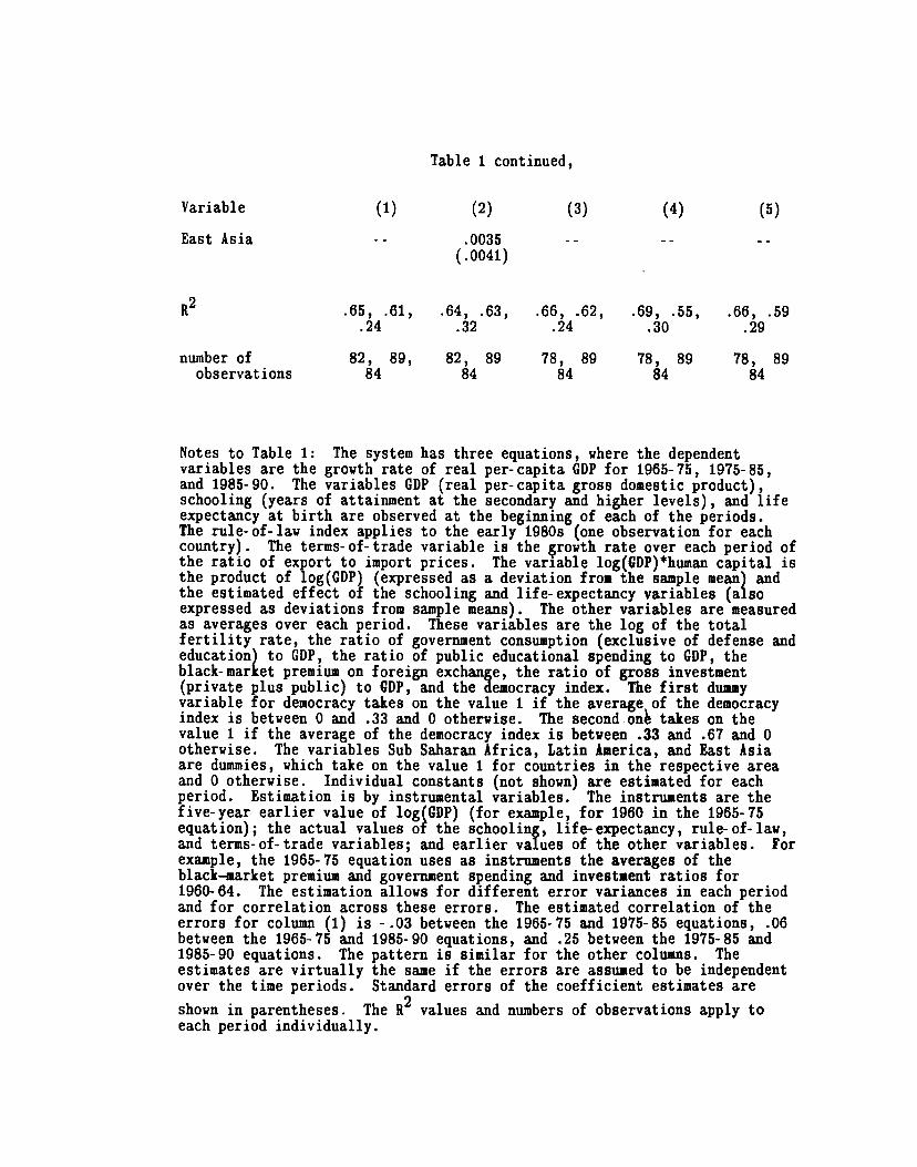
Table 1 continued,
Variable (1) (2) (3) (4) (5)
East Asia .0035
(.0041)
It2 .65, .61, .64, .63, .66, .62, .69, .55, .66, .59.24 .32 .24 .30 .29
number of 82, 89, 82, 89 78, 89 78, 89 78, 89observations 84 84 84 84 84
Notes to Table 1: The system has three equations, where the dependentvariables are the growth rate of real per-capita GDP for 1965-75, 1975-85,and 1985-90. The variables GDP (real per-capita gross domestic product),schooling (years of attainment at the secondary and higher levels), and lifeexpectancy at birth are observed at the beginning of each of the periods.The rule-of-law index applies to the early 1980s (one observation for eachcountry). The terms-of-trade variable is the rowth rate over each period ofthe ratio of export to import prices. The variable log(GDP)*huinan capital isthe product of log(GDP) (expressed as a deviation from the sample mean) andthe estimated effect of the schooling and life-expectancy variables (alsoexpressed as deviations from sample means). The other variables are measuredas averages over each period. These variables are the log of the totalfertility rate, the ratio of government consumption (exclusive of defense andeducation) to GDP, the ratio of public educational spending to GDP, theblack-market premium on foreign exchange, the ratio of gross investment(private plus public) to GDP, and the democracy index. The first dummyvariable for democracy takes on the value 1 if the average of the democracyindex is between 0 and .33 and 0 otherwise. The second on takes on thevalue 1 if the average of the democracy index is between .33 and .67 and 0otherwise. The variables Sub Saharan Africa, Latin America, and East Asiaare dummies, which take on the value 1 for countries in the respective areaand 0 otherwise. Individual constants (not shown) are estimated for eachperiod. Estimation is by instrumental variables. The instruments are thefive-year earlier value of log(GDP) (for example, for 1960 in the 1965-75equation); the actual values of the schooling, life-expectancy, rule-of-law,and terms-of-trade variables; and earlier values of the other variables. Forexample, the 1965-75 equation uses as instruments the averages of theblack—market premium and government spending and investment ratios for1960-64. The estimation allows for different error variances in each periodand for correlation across these errors. The estimated correlation of theerrors for column (1) is - .03 between the 1965-75 and 1975-85 equations, .06between the 1965-75 and 1985-90 equations, and .25 between the 1975-85 and1985-90 equations. The pattern is similar for the other columns. Theestimates are virtually the same if the errors are assumed to be independentover the time periods. Standard errors of the coefficient estimates are
shown in parentheses. The It2 values and numbers of observations apply to
each period individually.
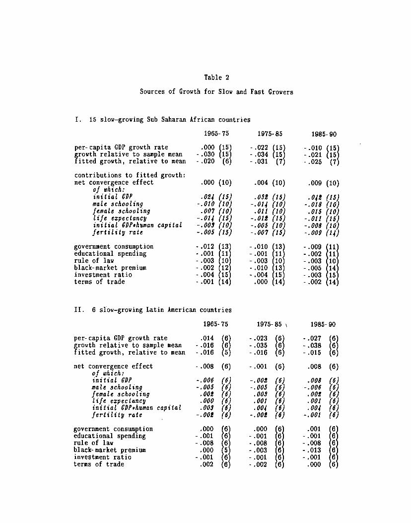
Table 2
Sources of Growth for Slow and Fast Growers
I. 15 slow—growing Sub Saharan African countries
1965-75 1975-85
II. 6 slow—growing Latin American countries
1985- 90
per-capita GOP growth rategrowth relative to sample meanfitted growth, relative to mean
.000 (15- .030 (15- .020 (6
- .022 (15- .034 (15- .031 (7
- .010 (15- .021 (15- .025 (7
contributions to fitted growth:net convergence effect
of which:initial CDPmale schoolingfemale schoolinglife expectancyinitial CDI'*human capital
fertility rate
.000 (10)
.024 (15)-.010 (10).007 (10)
-. 014 (15)-. 003 (10)-.005 (15)
.004 (10)
.032 (15)-. 014 (10).011 (10)
-. 012 (15)-. 005 (10)-.007 (15)
.009 (10)
.042 (15)-. 018 (10).015 (10)
-.011 (15)-.008 (10)-.009 (14)
government consumptioneducational spendingrule of law
- .012 13- .001 11- .003 10
- .010 13- .001 11- .003 10
- .009 11- .002 11- .003 10
black-market premium - .002 12 - .010 13 - .005 14investment ratio - .004 15 - .004 15 - .003 15terms of trade - .001 14 .000 14 - .002 14
1965-75 1975-85 1985-90
per-capita GOP growth rate .014 6 - .023 6 - .027 6growth relative to sample meanfitted growth, relative to mean
- .016 6- .016 5
- .035 6- .016 6
- .038 6- .015 6
net convergence effectof which:initial CD?male schoolingfemale schoolinglife expectancyinitial CDP*human capital
fertility rate
- .008(6)
-.006 (6)-.005 (6).002 (6).000 (6).003 (6)
-.002 (6)
- .001 (6)
-.002 (6)-.005 (6).003 (6).001 (6).004 (6)
-.002 (6)
.008 (6)
.008 (6)-. 006 (6).002 (6).001 (6).004 (6)
-.001 (6)
government consumption .000 6 .000 6 .001 6educational spendingrule of law
- .001 6- .008 6
- .001 6- .008 6
- .001 6- .008 6
black-market premium .000 5 - .003 6 - .013 6investment ratio - .001 6 - .001 6 - .001 6terms of trade .002 6 - .002 6 .000 6

Table 2, continued
HI. 9 fast—growing East Asian countries
1965- 75 1975- 85 1985- 90
IV. 6 fast—growing European countries
1965- 75 1975- 85 1985- 90
per-capita GDP growth rategrowth relative to sample meanfitted growth, relative to mean
.059
.028
.031
998
.052
.040
.031
998
.058
.047
.022
998
net convergence effectof which:initial CD?
male schoolingfemale schoolinglife expectancyinitial CDI'*human capital
fertility rate
.019
.004
.008
.000
.002
.003
.001
(8)
(8)
(8)
(8)
(9)
(8)
(9)
.012
-.002.007.000
.004
.001
.005
(8)
(9)
(8)
(8)
(9)
(8)
(9)
.001
-.013.012
-.005
.004-.001.007
(8)
(9)
(8)
(8)
(9)
(8)
(9)
government consumptioneducational spendingrule of law
-.004.001
.005
888
-.006.001
.005
888
.007- .001.005
888
black-market premium .002 8 .004 8 .005 8investment ratio .001 9 .003 9 .003 9terms of trade .001 9 .000 9 .001 9
per-capita GDP growth rategrowth relative to sample meanfitted growth, relative to mean
.050
.020
.019
666
.026
.014
.013
666
.038
.027
.013
666
net convergence effectof which:initial CD?
male schoolingfemale schoolinglife expectancyinitial CDF#human capitalfertility rate
.004
-.017.002
-.002.010.002.009
(6)
(6)
(6)(6)(6)(6)(6)
-
-.
.004
-.023.002002.009.001.009
(6)
(6)
(6)(6)(6)(6)(6)
- .007
-.028.007
-.005.008.001.011
(6)
(6)
(6)(6)(6)(6)(6)
government consumptioneducational spendingrule of lawblack-market premiuminvestment ratioterms of trade
.004
.000
.006
.003
.004- .001
666666
.004
.000
.006
.004
.003
.000
666666
.003- .001.006.006.002.004
666866

Notes to Table 2: The roups of countries are selected from those in thelowest or highest quintile of growth rates of real per—capita GDP from 1965to 1990. The 15 slow-growing Sub Saharan African countries are (in
increasing order of growth rates) Chad, Mozambique, Madagascar, Zambia,Uganda, Zaire, Somalia, Benin, Niger, Mauritania, Comoros, Central AfricanRepublic, Sierra Leone, Ghana, and Sudan. The six slow-growing LatinAmerican countries are Nicaragua, Guyana, Venezuela, Peru, Haiti, andArgentina. The nine fast-growing East Asian countries (in decreasing orderof growth rates) are South Korea, Singapore, Taiwan, Hong Kong, China,Indonesia, Japan, Thailand, and Malaysia. The six fast-growing Europeancountries are Malta (included with Europe), Portugal, Ireland, Italy, Greece,and Finland. Fitted values are from the growth—rate regression shown incolumn (1) of Table 1. The figure in parentheses is the number ofobservations over which the value is averaged (reflecting the availability ofdata). The fitted values (expressed as deviations from sample means) arebroken down into components, which correspond to the explanatory variables inthe regression. See the text and the notes to Table 1 for definitions ofvariables. The net convergence term encompasses the effects from initialreal per—capita GDP, male and female secondary and. higher school attainment,life expectancy, the interaction between initial real per-capita GOP andhuman capital (schooling and life expectancy), and the fertility rate. Sincethe rule—of—law index has only one observation per country, the estimatedcontribution from this variable does not vary over time.
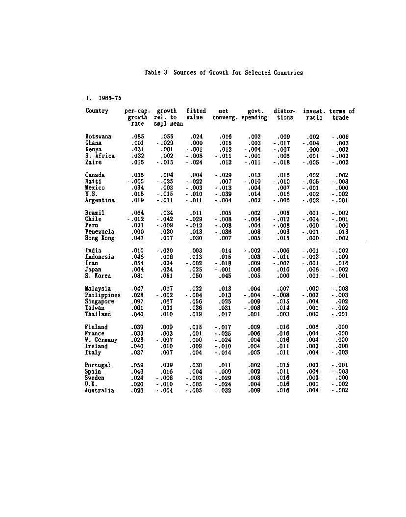
Table 3 Sources of Growth for Selected Countries
I. 1965-75
Country per-cap. growth fitted net govt. distor- invest, terms ofgrowth rel. to value converg. spending tions ratio traderate smpl mean
.085 .055 .024 .016 .002 .009 .002 - .006
.001 - .029 .000 .015 .003 - .017 - .004 .003
.031 .001 - .001 .012 - .004 - .007 .000 - .002
.032 .002 - .008 - .011 - .001 .005 .001 - .002
.015 - .015 - .024 .012 - .011 - .018 - .005 - .002
.035 .004 .004 - .029 .013 .016 .002 .002- .005 - .035 - .022 .007 - .010 - .010 - .005 - .003.034 .003 - .003 - .013 .004 .007 - .001 .000.015 - .015 - .010 - .039 .014 .016 .002 - .002.019 - .011 - .011 - .004 .002 - .006 - .002 - .001
.064 .034 .011 .005 .002 .005 .001 - .002- .012 - .042 - .029 - .008 - .004 - .012 - .004 - .001.021 - .009 - .012 - .008 .004 - .008 .000 .000.000 - .030 - .013 - .036 .008 .003 - .001 .013.047 .017 .030 .007 .005 .015 .000 .002
.010 - .020 .003 .014 - .002 - .006 - .001 - .002
.046 .016 .013 .015 .003 - .011 - .003 .009
.054 .024 - .002 - .018 .009 - .007 - .001 .016
.064 .034 .025 - .001 .006 .016 .006 - .002
.081 .051 .050 .045 .005 .000 .001 - .001
.047 .017 .022 .013 .004 .007 .000 - .003
.028 - .002 - .004 .013 - .004 - .d08 - .002 - .003
.097 .067 .056 .025 .009 .015 .004 .002
.061 .031 .036 .031 - .008 .014 .001 - .002
.040 .010 .019 .017 .001 .003 .000 - .001
.039 .009 .015 - .017 .009 .016 .006 .000
.033 .003 .001 - .025 .006 .016 .004 .000
.023 - .007 .000 - .024 .004 .016 .004 .000
.040 .010 .009 - .010 .004 .011 .003 .000
.037 .007 .004 - .014 .005 .011 .004 - .003
Portugal .059 .029 .030 .011 .002 .015 .003 - .001Spain .046 .016 .004 - .009 .002 .011 .004 - .003Sweden .024 - .006 - .003 - .029 .008 .016 .003 .000U.K. .020 - .010 - .005 - .024 .004 .016 .001 - .002Australia .026 - .004 - .005 - .032 .009 .016 .004 - .002
BotswanaGhana
KenyaS. AfricaZaire
CanadaHaitilexicoU.S.
Argentina
BrazilChilePeruVenezuela
Hong Kong
IndiaIndonesiaIran
JapanS. Korea
Jalays ia
PhilippinesSingaporeTaiwanThailand
FinlandFranceV. GermanyIreland
Italy
II. 1975-85
Table 3, continued
Country per-cap. growth fitted net govt. diator- invest. terms ofgrowth rel. to value converg. spending tions ratio traderate sinpi mean
India .023 .011 .028 .032 - .002 .001Indonesia .055 .044 .019 .019 - .001 - .005Iran - .023 - .034 - .020 - .019 .010 - .022Japan .034 .022 .017 - .015 .010 .017S. Korea .061 .049 .050 .035 .009 .003
Finland .021France .015
V. Germany .021
Ireland .023
Italy .027
.010 .009 - .021 .007 .017
.004 .005 - .024 .008 .017
.010 .006 - .018 .005 .017
.011 .013 - .012 .008 .013
.015 .006 - .014 .004 .013
.005 .000
.003 .001
.003 .000
.003 .001
.002 .001
.002 - .001
.002 .000
.001 .000
.000 .003
.003 - .002
Botswana .051 .040 .003 .002 - .003 .007Ghana - .015 - .026 - .037 .031 - .010 - .051Kenya - .006 - .017 .005 .010 - .003 - .003S. Africa - .004 - .016 - .010 - .012 - .001 .005Zaire - .035 - .047 - .019 .014 - .005 - .025
Canada .024 .012 .005 - .029 .014 .017Haiti .007 - .004 - .003 .016 - .009 - .008Mexico .013 .002 .006 - .010 .005 .006U.S. .021 .009 .005 - .029 .015 .017
Argentina - .014 - .026 - .013 - .007 .006 - .007
Brazil .013 .002 - .001 - .005 .003 .003Chile .011 .000 .005 .004 - .003 .010Peru - .018 - .029 - .006 - .002 .001 - .003Venezuela - .019 - .031 - .008 - .025 .008 .000
Hong Kong .065 .053 .026 .002 .006 .017
.003 - .005-.004 -.002- .001 .002.001 - .003
- .004 .001
.002 .000- .003 .002.000 .004.001 .001
-.001 -.005
.001 - .004-.002 -.004.001 - .004.001 .008.001 - .001
.000 - .003
.001 .005
.002 .008
.005 - .001
.003 - .001
.003 .003
.000 - .006
.006 .002
.003 - .002
.000 - .003
Malaysia .044 .033 .039 .013 .010 .009
Philippines - .006 - .018 - .004 .014 - .007 - .006Singapore .049 .037 .040 .004 .010 .017Taiwan .057 .046 .034 .020 - .003 .017Thailand .037 .026 .020 .017 .001 .004
Portugal .014 .003 .019 .003 .001 .015
Spain .002 - .010 .006 - .013 .004 .013Sweden .012 .000 - .001 - .027 .007 .017U.K. .021 .010 .008 - .018 .006 .017Australia .016 .005 .001 - .028 .011 .017
III. 1985-90
Table 3, continued
.055
.013
.033- .010- .025
.045
.002
.022
.020- .036
- .004.034.019
- .007.027
- .006- .016- .002.002
- .005
009- .009.000.008
- .005
.021- .029
.003
.021- .021
.010- .040- .007.010
- .031
- .008- .001- .002.010
- .034.016
- .008- .037- .002
.014
.011
.004
.017
.007
.019- .022.007.019
- .007
- .002.042
- .039- .009.060
- .013.031
- .050- .020.050
.001
.001- .003.001.001
.006
.027
.008
.023
.010
- .006.006.011
- .016- .018
.004
.004
.003
.009
.006
.000
.011
.001
.014
.019
.034
.035
.052
.042
.087
.000
.001
.000
.000
.001
.024
.025
.062
.032
.076
.008
.007- .007.000.002
.042
.007
.052
.019
.044
.040
.014- .007- .023.020
- .003- .003.007.010.012
.004- .005- .056.019.005
Country per-cap. growth fitted net govt. distor- invest, terms ofgrowth rel. to value converg. spending tions ratio traderate smpl mean
Botswana -- .000Ghana - .002 - .004Kenya .013 - .001S. Africa - .003 .000Zaire .024 - .003
Canada .003 .004Haiti - .018 - - .003Mexico - .002 - .001U.s. .002 .002
Argentina- .003 - .003
BrazilChile -
PeruVenezuela - -Hong Kong
IndiaIndonesia -
Iran - - -
JapanS. Korea
MalaysiaPhilippines -
Singapore -
TaiwanThailand
FinlandFranceV. GermanyIrelandItaly
PortugalSpainSwedenU.K.Australia -
Notes to Table 3: See the notes to Tables 1 and 2. The growth rate is for per-capita real GDP. The net convergence term is the combination of the effects frominitial real per-capita GDP, male and female school attainment at the secondary and
higher levels, li expectancy at birth, and fertility. The government spendin termcombines the effects of government consumption (exclusive of defense and education)and public educational spending. The distortions term includes the rule-of-law indexand the black-market premium on foreign exchange.
.037
.028
.059
.077
.075
.000
.004
.002
.006
.005
.026
.017
.048
.067
.064
.001
.003
.003
.007
.002
.025
.008
.025
.025
.025
.004
.017
.012
.008
.014
.012- .006.011
- .002.001
.010- .004.019
.018
.006
.032
.027
.029
.046
.028
.003
.001
.006
.003
.001
.021
.016
.018
.035
.018
- .004.001.001
- .001003
.010
.009
.010
.012
.007
- .025- .026- .023- .014- .017
.006
.009
.005
.008
.002
.019
.019
.019
.015
.015
.052
.049
.017
.032
.009
.005
.003
.003
.002
.003
.041
.039
.006
.021
.001
.004
.003
.005
.001
.005
.030
.022
.000
.004
.005
.006- .005- .030- .023- .030
- .001.004.006.005.010
.017
.015
.019
.019
.019
.001
.003
.002
.001
.004
.006
.004
.003
.002
.002
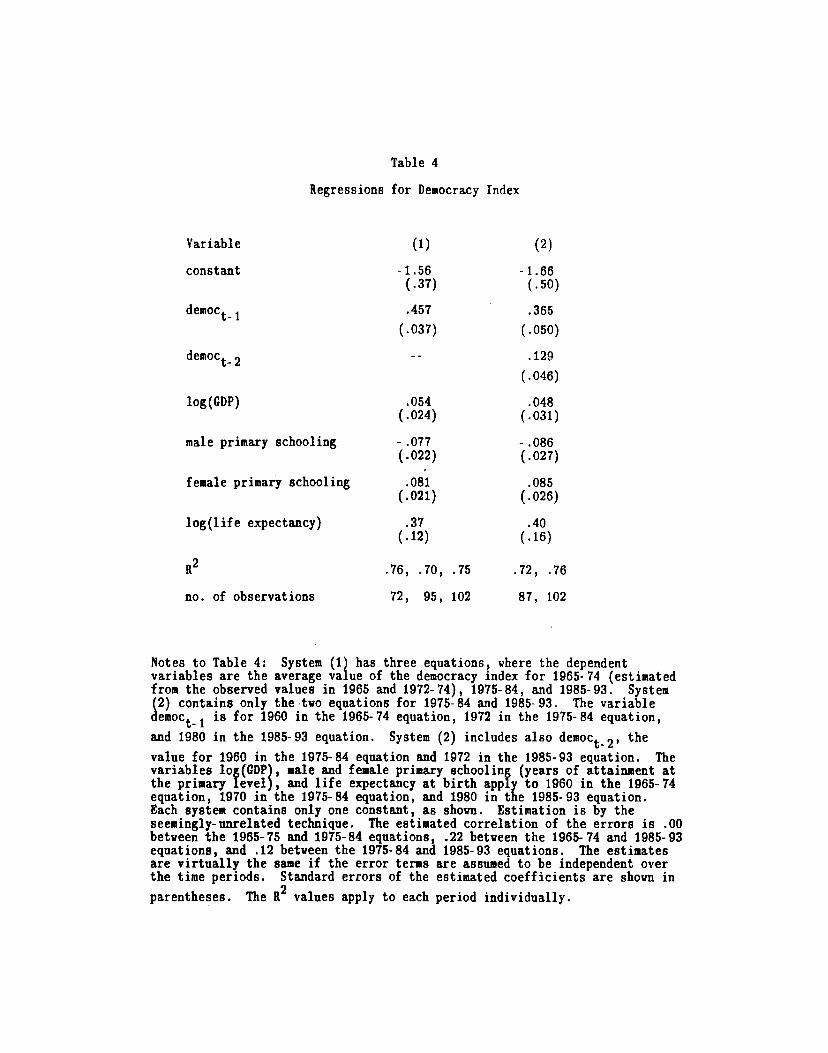
Table 4
Regressions for Democracy Index
Variable (1) (2)
constant -1.56 -1.66
(.37) (.50)
democti .365
(.037) (.050)
democt2 .129
(.046)
log(GDP) .054 .048
(.024) (.031)
male primary schooling - .077 - .086(.022) (.027)
female primary schooling .081 .085
(.021) (.026)
log(life expectancy) .37 .40
(.12) (.16)
.76, .70, .75 .72, .76
no. of observations 72, 95, 102 87, 102
Notes to Table 4: System (1) has three equations, where the dependentvariables are the average value of the democracy index for 1965- 74 (estimatedfrom the observed values in 1965 and 1972-74), 1975-84, and 1985-93. System(2) contains only the two equations for 1975-84 and 1985-93. The variabledemocti is for 1960 in the 1965-74 equation, 1972 in the 1975-84 equation,
and 1980 in the 1985-93 equation. System (2) includes also denloc2, the
value for 1960 in the 1975-84 equation and 1972 in the 1985-93 equation. Thevariables log(GDP), male and female primary schooling (years of attainment atthe primary level), and life expectancy at birth apply to 1960 in the 1965- 74equation, 1970 in the 1975-84 equation, and 1980 in the 1985-93 equation.Each system contains only one constant, as shown. Estimation is by theseemingly-unrelated technique. The estimated correlation of the errors is .00between the 1965- 75 and 1975-84 equations, .22 between the 1965- 74 and 1985- 93
equations, and .12 between the 1975-84 and 1985-93 equations. The estimatesare virtually the same if the error terms are assumed to be independent overthe time periods. Standard errors of the estimated coefficients are shown inparentheses. The R2 values apply to each period individually.
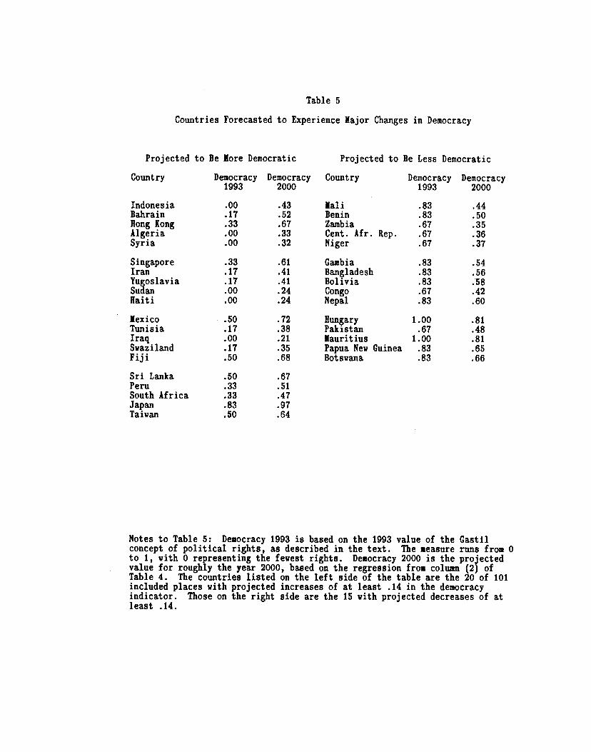
Table 5
Countries Forecasted to Experience Major Changes in Democracy
Projected to Be More Democratic Projected to Be Less Democratic
Country Democracy Democracy Country Democracy Democracy1993 2000 1993 2000
Indonesia .00 .43 Mali .83 .44Bahrain .17 .52 Benin .83 .50
Hong Hong .33 .67 Zambia .67 .35
Algeria .00 .33 Cent. Afr. Rep. .67 .36
Syria .00 .32 Niger .67 .37
Singapore .33 .61 Gambia .83 .54Iran .17 .41 Ba.nladesh .83 .56
Yugoslavia .17 .41 Bolivia .83 .58Sudan .00 .24 Congo .67 .42Haiti .00 .24 Nepal .83 .60
Mexico .50 .72 Hungary 1.00 .81Tunisia .17 .38 Pakistan .67 .48
Iraq .00 .21 Mauritius 1.00 .81Swaziland .17 .35 Papua New Guinea .83 .65
Fiji .50 .68 Botsvana .83 .66
Sri Lanka .50 .67Peru .33 .51
South Africa .33 .47
Japan .83 .97Taiwan .50 .64
Notes to Table 5: Democracy 1993 is based on the 1993 value of the Gastilconcept of political rights, as described in the text. The measure runs from 0to 1, with 0 representing the fewest rights. Democracy 2000 is the projectedvalue for roughly the year 2000, based on the regression from column (2) ofTable 4. The countries listed on the left side of the table are the 20 of 101included places with projected increases of at least .14 in the democracyindicator. Those on the right side are the 15 with projected decreases of atleast .14.
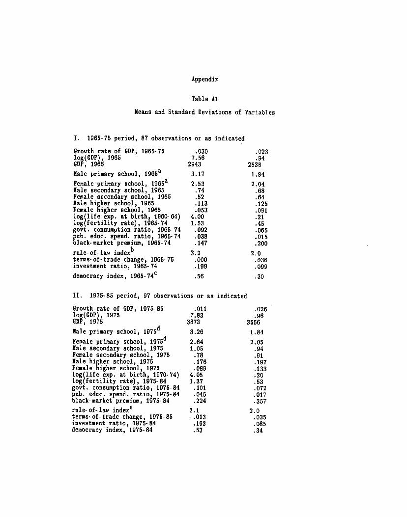
Appendix
Table Al
Means and Standard Deviations of Variables
I. 1965-75 period, 87 observations or as indicated
Growth rate of GDP, 1965-75 .030 .023log(GDP), 1965 7.56 .94GOP, 1965 2943 2838
Male primary school, 1965a 3.17 1.84
Female primary school, 1965a 2.53 2.04Male secondary school, 1965 .74 .68Female secondary school, 1965 .52 .64Male higher school, 1965 .113 .125Female higher school, 1965 .053 .091
log(life exp. at birth, 1960-64) 4.00 .21
log(fertility rate), 1965-74 1.53 .45
govt. consumption ratio, 1965-74 .092 .065
pub. educ. spend. ratio, 1965-74 .038 .015black-market premium, 1965-74 .147 .200
rule-of-law indexb 3.2 2.0terms-of-trade change, 1965-75 .000 .036investment ratio, 1965-74 .199 .099
democracy index, l96574 .56 .30
II. 1975-85 period, 97 observations or as indicated
Growth rate of CUP, 1975-85 .011 .026log(GDP), 1975 7.83 .96GOP, 1975 3873 3556
Male primary school, l975 3.26 1.84
Female primary school, 1975d 2.64 2.05Male secondary school, 1975 1.05 .94
Female secondary school, 1975 .78 .91
Male higher school, 1975 .176 .197Female higher school, 1975 .089 .133log(life exp. at birth, 1970-74) 4.05 .20log(fertility rate), 1975-84 1.37 .53
govt. consumption ratio, 1975-84 .101 .072pub. educ. spend. ratio, 1975-84 .045 .017black-market premium, 1975-84 .224 .357
rule-of-law indexe 3.1 2.0terms-of-trade change, 1975-85 - .013 .035investment ratio, 1975-84 .193 .085
democracy index, 1975-84 .53 .34
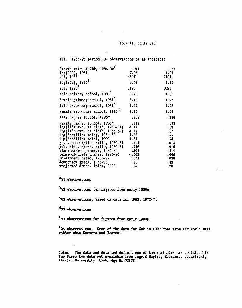
Table Al, continued
III. 1985-95 period, 97 observations or as indicated
Growth rate of GDP, i985go .011 .033
log(GDP), 1985 7.95 1.04GDP, 1985 4597 4404
log(GDP), l99O 8.02 1.10
GDP, 5193 5091
Male primary school, 1985d 3.79 1.68
Female primary school, 1985 3.10 1.96
Male secondary school, 1985d 1.42 1.08
Female secondary school, 1985d 1.10 1.04
Male higher school, 1985d .268 .246
Female higher school, 1985d .159 .193
log life exp. at birth, 1980-84) 4.12 .18
log life exp. at birth, 1985-89) 4.15 .17
log fertility rate), 1985-89 1.26 .55
log fertility rate), 1990 1.23 .54
govt. consumption ratio, 1980-84 .101 .074
pub. educ. spend. ratio, 1980-84 .046 .018black-market premium, 1985-89 .301 .514terms- of- trade change, 1985-90 - .009 .046investment ratio, 1985-89 .171 .086
democracy index, 1985-93 .61 .33projected democ. index, 2000 .65 .28
a81 observations
b82 observations for figures from early 1980s.
C83 observations, based on data for 1965, 1972-74.
d96 observations.
e89 observations for figures from early 1980s.
observations. Some of the data for GDP in 1990 come from the Vorld Bank,rather than Summers and Heston.
Notes: The data and detailed definitions of the variables are contained inthe Barro-Lee data set available from Ingrid Sayied, Economics Department,Harvard University, Cambridge MA 02138.
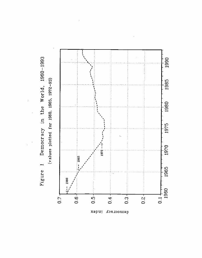
Figu
re
1 D
emoc
racy
in
the
Wor
ld,
1960
—19
93
(val
ue!
plot
ted
for
1960
, 19
65,
1972
—93
)
1960
• -
I I
1960
19
65
I I
P
I I
I I
1970
19
75
1980
I
1985
19
90
0.7
0.6
0.5
0.4
0.3-
0.2
C.)
C.)
0
• I'
• .
• .
. —
• '.
. .
. •
. .
—'—
1— —
—
1972
——
>'_
_.,
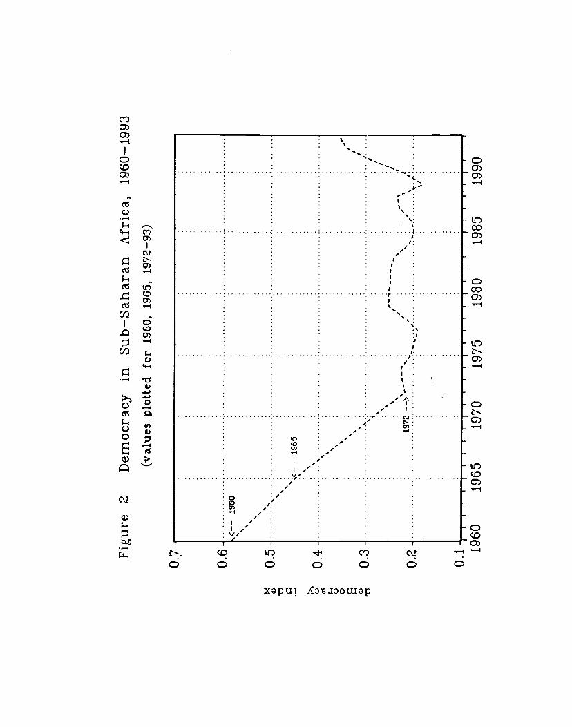
Figu
re
2 D
emoc
racy
in
Su
b—Sa
hara
n A
fric
a,
1960
—19
93
(val
ues
plot
ted
for
1960
, 19
65,
1972
—93
)
'h(
196
S S
•
S
• S
•
S S
-S S
S S
S...
-S
. • 5
. /
. .
1972
——
>'..
/
S-S
..___
...,
0.1—
,
I I
I I
I I
I I
1960
19
65
1970
19
75
1980
19
85
1990
0.7
0.6
<"
1960
:
• :
S
0.5
. k —
4
I:) 0 0 1)
0.4
0.3
0.2
/ •
I F
/ I •
F I
.1
•1
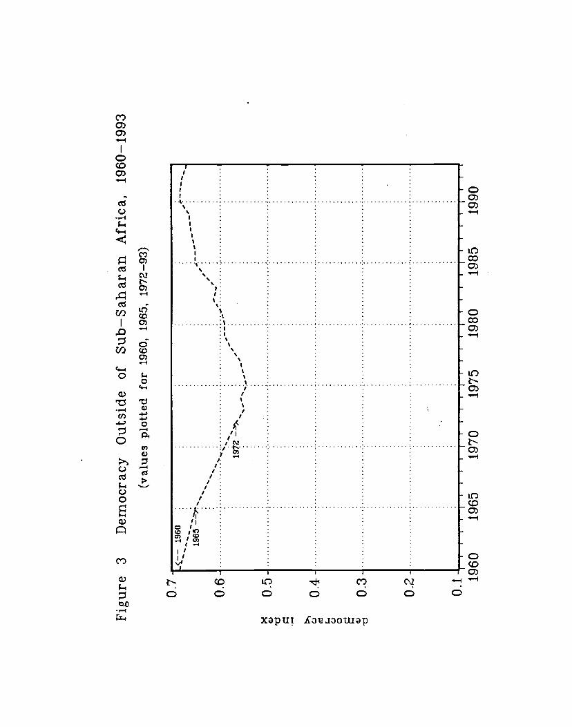
Figu
re
3 D
emoc
racy
O
utsi
de
of
Sub—
Saha
ran
Afr
ica,
19
60—
1993
(val
ues
plot
ted
for
1960
, 19
65,
1972
—93
)
O.7
-<6o
19
6 —
0
0.6
-
I :: 0.
2 0
. .
.
I I
I I
I I
I I
I I
1 I
I I
I I
I I
I I
I I
1960
19
65
1970
19
75
1980
19
85
1990
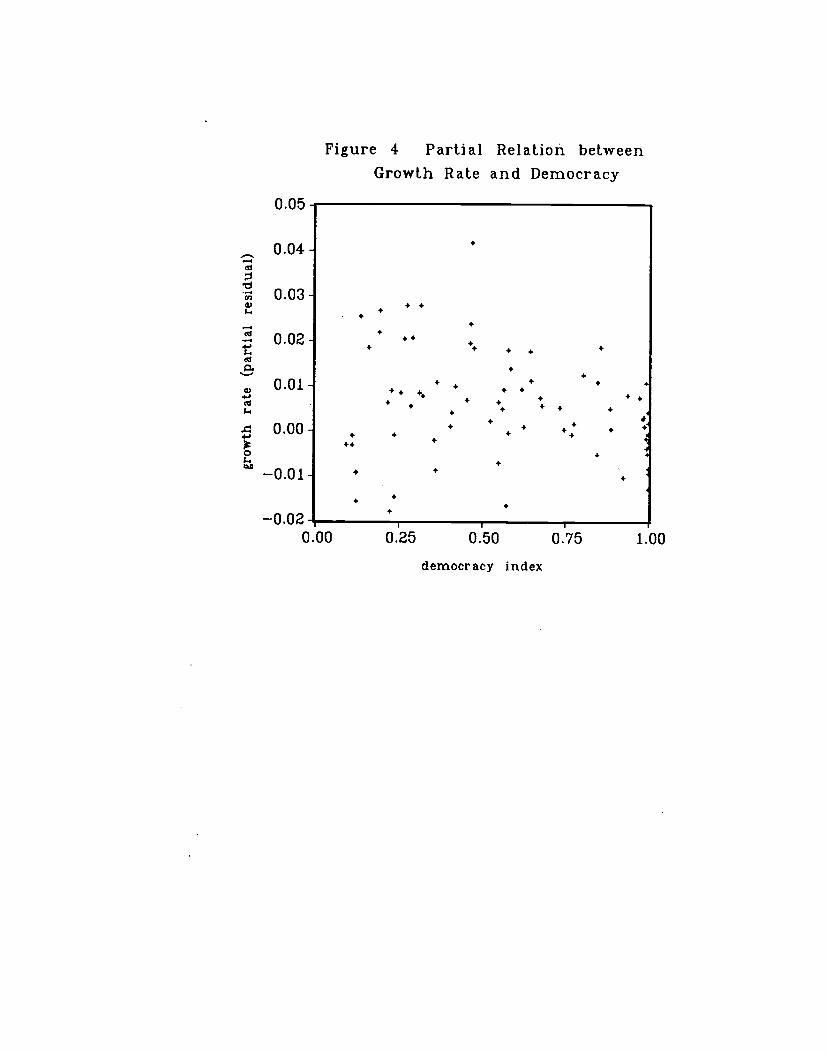
Figure 4 Partial Relation betweenGrowth Rate and Democracy
0.05•
- 0.04
0.03+ + +
• ++
002 ++• + + • +
++
+++ + ++ +
+ • +4+ + + 4 + +4
0.00 + ++ +
+ + 4 + ++ 4
++ +o 4
++ +
+
+ ++
+—0.02 I I
0.00 0.25 0.50 0.75 1.00
democracy index