NBER WORKING PAPER SERIES

DEMAND-BASED OPTION PRICING

Nicolae GarleanuLasse Heje PedersenAllen M. Poteshman

Working Paper 11843http://www.nber.org/papers/w11843

NATIONAL BUREAU OF ECONOMIC RESEARCH1050 Massachusetts Avenue

Cambridge, MA 02138December 2005

We are grateful for helpful comments from David Bates, Nick Bollen, Oleg Bondarenko, Menachem Brenner,Andrea Buraschi, Josh Coval, Apoorva Koticha, Sophie Ni, Jun Pan, Neil Pearson, Mike Weisbach, JoshWhite, and especially from Steve Figlewski, as well as from seminar participants at the Caesarea CenterConference, Columbia University, Harvard University, HEC Lausanne, the 2005 Inquire Europe Conference,London Business School, the 2005 NBER Behavioral Finance Conference, the 2005 NBER UniversitiesResearch Conference, the NYU-ISE Conference on the Transformation of Option Trading, New YorkUniversity, Oxford University, Stockholm Institute of Financial Research, Texas A&M University, theUniversity of Chicago, University of Illinois at Urbana-Champaign, the University of Pennsylvania,University of Vienna, and the 2005 WFA Meetings. The views expressed herein are those of the author(s)and do not necessarily reflect the views of the National Bureau of Economic Research.

©2005 by Nicolae Garleanu, Lasse Heje Pedersen, and Allen M. Poteshman. All rights reserved. Shortsections of text, not to exceed two paragraphs, may be quoted without explicit permission provided that fullcredit, including © notice, is given to the source.

Demand-Based Option PricingNicolae Garleanu, Lasse Heje Pedersen, and Allen M. PoteshmanNBER Working Paper No. 11843December 2005JEL No. G0, G12, G13, G14, G2

ABSTRACT

We model the demand-pressure effect on prices when options cannot be perfectly hedged. The model

shows that demand pressure in one option contract increases its price by an amount proportional to

the variance of the unhedgeable part of the option. Similarly, the demand pressure increases the price

of any other option by an amount proportional to the covariance of their unhedgeable parts.

Empirically, we identify aggregate positions of dealers and end users using a unique dataset, and

show that demand-pressure effects help explain well-known option-pricing puzzles. First, end users

are net long index options, especially out-of-money puts, which helps explain their apparent

expensiveness and the smirk. Second, demand patterns help explain the prices of single-stock

options.

Nicolae GarleanuWharton School of BusinessUniversity of Pennsylvania3620 Locust WalkPhiladelphia, PA 19104garleanu@wharton.upenn.edu

Lasse Heje PedersenNYU Stern Finance44 West Fouth StreetSuite 9-190New York, NY 10012and NBERlpederse@stern.nyu.edu

Allen M. PoteshmanUniversity of Illinois at Urbana-Champaign340 Wohlers Hall1206 South Sixth StreetChampaign, IL 61820poteshma@uiuc.edu

1 Introduction

“[Option implied volatility] skew is heavily influenced by supply and de-mand factors.”— Gray, director of global equity derivatives, Dresdner Kleinwort Benson

“The number of players in the skew market is limited. ... there’s a hugeimbalance between what clients want and what professionals can provide.”— Belhadj-Soulami, head of equity derivatives trading for Europe, Paribas

“To blithely attribute divergences between objective and risk-neutral prob-ability measures to the free ‘risk premium’ parameters within an affinemodel is to abdicate one’s responsibilities as a financial economist. ... a re-newed focus on the explicit financial intermediation of the underlying risksby option market makers is needed.”— Bates (2003)

We take on this challenge by providing a model of option intermediation, and byshowing empirically using a unique dataset that demand pressure can help explain themain option-pricing puzzles.

The starting point of our analysis is that options are traded because they are usefuland, therefore, options cannot be redundant for all investors (Hakansson (1979)). Wedenote the agents who have a fundamental need for option exposure as “end users.”

Intermediaries such as market makers and proprietary traders provide liquidity toend users by taking the other side of the end-user net demand. If intermediaries canhedge perfectly — as in a Black and Scholes (1973) and Merton (1973) economy —then option prices are determined by no-arbitrage and demand pressure has no effect.In reality, however, even intermediaries cannot hedge options perfectly because of theimpossibility of trading continuously, stochastic volatility, jumps in the underlying, andtransaction costs (Figlewski (1989)).1

To capture this effect, we depart from the standard no-arbitrage literature thatfollows Black-Scholes-Merton by considering explicitly how options are priced by com-petitive risk-averse dealers who cannot hedge perfectly. In our model, dealers trade anarbitrary number of option contracts on the same underlying at discrete times. Sincethe dealers trade many option contracts, certain risks net out, while others do not. Thedealers can hedge part of the remaining risk of their derivative positions by trading theunderlying security and risk-free bonds. We consider a general class of distributionsfor the underlying, which can accommodate stochastic volatility and jumps. Dealerstrade with end users. The model is agnostic about the end users’ reasons for trade.

We compute equilibrium prices as functions of demand pressure, that is, the pricesthat make dealers optimally choose to supply the options that the end users demand.

1Also, traders have capital constraints as emphasized, e.g., by Shleifer and Vishny (1997).

2

We show explicitly how demand pressure enters into the pricing kernel. Intuitively,a positive demand pressure in an option increases the pricing kernel in the states ofnature in which an optimally hedged position has a positive payoff. This pricing-kerneleffect increases the price of the option, which entices the dealers to sell it. Specifically,a marginal change in the demand pressure in an option contract increases its price byan amount proportional to the variance of the unhedgeable part of the option, wherethe variance is computed under a certain probability measure. Similarly, the demandpressure increases the price of any other option by an amount proportional to thecovariance of their unhedgeable parts. Hence, while demand pressure in a particularoption raises its price, it also raises the price of other options on the same underlying,especially similar contracts.

Empirically, we use a unique dataset to identify aggregate daily positions of dealersand end users. In particular, we define dealers as market makers and end users asproprietary traders and customers of brokers.2 We find that end users have a net longposition in S&P500 index options with large net positions in out-of-the-money puts.Hence, since options are in zero net supply, dealers are short index options. While itis conventional wisdom among option traders that Wall Street is short index volatility,this paper is the first to demonstrate this fact using data on option holdings. Thiscan help explain the puzzle that index options appear to be expensive, and that low-moneyness options seem to be especially expensive (Longstaff (1995), Bates (2000),Coval and Shumway (2001), Amin, Coval, and Seyhun (2004), Bondarenko (2003)). Inthe time series, demand for index options is related to their expensiveness, measuredby the difference between their implied volatility and the volatility measure of Bates(2005). Further, the steepness of the smirk, measured by the difference between theimplied volatility of low-moneyness options and at-the-money options, is positivelyrelated to the skew of option demand, measured by the demand for low-moneynessoptions minus the demand for high-moneyness options.

Jackwerth (2000) finds that a representative investor’s option-implied utility func-tion is inconsistent with standard assumptions in economic theory.3 Since options arein zero net supply, a representative investor holds no options. We reconcile this findingfor dealers who have significant short index option positions. Intuitively, an investorwill short index options, but only a finite number of options. Hence, while a standard-utility investor may not be marginal on options given a zero position, he is marginalgiven a certain negative position. We do not address why end users buy these op-tions; their motives might be related to portfolio insurance and agency problems (e.g.between investors and fund managers) that are not well captured by standard utilitytheory.

Another option-pricing puzzle is that index option prices are so different from theprices of single-stock options despite the fact that the distributions of the underlying

2The empirical results are robust to classifying proprietary traders as either dealers or end users.3See also Driessen and Maenhout (2003).

3

appear relatively similar (e.g., Bakshi, Kapadia, and Madan (2003) and Bollen andWhaley (2004)). In particular, single-stock options appear cheaper and their smile isflatter. Consistently, we find that the demand pattern for single-stock options is verydifferent from that of index options. For instance, end users are net short single-stockoptions – not long, as in the case of index options.

Demand patterns further help explain the time-series and cross-sectional pricing ofsingle-stock options. Indeed, individual stock options are cheaper at times when endusers sell more options, and, in the cross section, stocks with more negative demandfor options, aggregated across contracts, tend to have relatively cheaper options.

The paper is related to several strands of literature. First, the literature on optionpricing in the context of trading frictions and incomplete markets derives bounds onoption prices. Arbitrage bounds are trivial with any transaction costs; for instance,the price of a call option can be as high as the price of the underlying stock (Soner,Shreve, and Cvitanic (1995)). This serious limitation of no-arbitrage pricing has ledCochrane and Saa-Requejo (2000) and Bernardo and Ledoit (2000) to derive tighteroption-pricing bounds by restricting the Sharpe ratio or gain/loss ratio to be below anarbitrary level, and stochastic dominance bounds for small option positions are derivedby Constantinides and Perrakis (2002) and extended and implemented empiricallyby Constantinides, Jackwerth, and Perrakis (2005). Rather than deriving bounds,we compute explicit prices based on the demand pressure by end users. We furthercomplement this literature by taking portfolio considerations into account, that is, theeffect of demand for one option on the prices of other options.

Second, the literature on utility-based option pricing (“indifference pricing”) derivesthe option price that would make an agent (e.g., the representative agent) indifferentbetween buying the option and not buying it. See Rubinstein (1976), Brennan (1979),Stapleton and Subrahmanyam (1984), Hugonnier, Kramkov, and Schachermayer (2005)and references therein. While this literature computes the price of the first “marginal”option demanded, we show how option prices change when demand is non-trivial.

Third, Stein (1989) and Poteshman (2001) provide evidence that option investorsmisproject changes in the instantaneous volatility of underlying assets by examiningthe price changes of shorter and longer maturity options. Our paper shows how thecognitive biases of option end users can translate (via their option demands) into op-tion prices even if market makers are not subject to any behavioral biases. By contrast,under standard models like Black-Scholes-Merton, market makers who can hedge theirpositions perfectly will correct the mistakes of other option market participants be-fore they affect option prices. As a result, this paper provides a foundation for theapplication of behavioral finance to the option market.

Fourth, the general idea of demand-pressure effects goes back, at least, to Keynes(1923) and Hicks (1939) who considered futures markets. Our model is the first to applythis idea to option pricing and to incorporate the important features of option markets,namely dynamic trading of many assets, hedging using the underlying and bonds,

4

stochastic volatility, and jumps. The generality of our model also makes it applicableto other markets. Consistent with our model’s predictions, Wurgler and Zhuravskaya(2002) find that stocks that are hard to hedge experience larger price jumps whenincluded into the S&P 500 index. Greenwood (2005) considers a major redefinition ofthe Nikkei 225 index in Japan and finds that stocks that are not affected by demandshocks, but that are correlated with securities facing demand shocks, experience pricechanges. Similarly in the fixed income market, Newman and Rierson (2004) find thatnon-informative issues of telecom bonds depress the price of the issued bond as wellas correlated telecom bonds, and Gabaix, Krishnamurthy, and Vigneron (2004) findrelated evidence for mortgage-backed securities. Further, de Roon, Nijman, and Veld(2000) find futures-market evidence consistent with the model’s predictions.

The most closely related paper is Bollen and Whaley (2004), which demonstratesthat changes in implied volatility are correlated with signed option volume. Theseempirical results set the stage for our analysis by showing that changes in optiondemand lead to changes in option prices while leaving open the question of whetherthe level of option demand impacts the overall level (i.e., expensiveness) of optionprices or the overall shape of implied-volatility curves.4 We complement Bollen andWhaley (2004) by providing a theoretical model and by investigating empirically therelationship between the level of end user demand for options and the level and overallshape of implied volatility curves. In particular, we document that end users tend tohave a net long SPX option position and a short equity-option position, thus helpingto explain the relative expensiveness of index options. We also show that there is astrong downward skew in the net demand of index but not equity options which helpsto explain the difference in the shapes of their overall implied volatility curves.

The rest of the paper is organized as follows. Section 2 describes the model, andSection 3 derives its pricing implications. Section 4 provides descriptive statistics ondemand patterns for options, Section 5 tests the effect of demand pressure on optionprices, and Section 6 concludes. The appendix contains proofs.

2 A Model of Demand Pressure

We consider a discrete-time infinite-horizon economy. There exists a risk-free assetpaying interest at the rate of Rf −1 per period, and a risky security that we refer to asthe “underlying” security. At time t, the underlying has an exogenous strictly positiveprice5 of St, dividend Dt, and an excess return of Re

t = (St + Dt)/St−1 − Rf and thedistribution of future prices and returns is characterized by a stationary Markov state

4Indeed, Bollen and Whaley (2004) find that a nontrivial part of the option price impact from dayt signed option volume dissipates by day t + 1.

5All random variables are defined on a probability space (Ω,F , P r) with an associated filtrationFt : t ≥ 0 of sub-σ-algebras representing the resolution over time of information commonly availableto agents.

5

variable Xt ∈ X ⊂ Rn, with X compact.6 (The state variable could include the current

level of volatility, the current jump intensity, etc.) The only condition we impose onthe transition function π : X × X → R+ of X is that it have the Feller property.

The economy further has a number of “derivative” securities, whose prices are tobe determined endogenously. A derivative security is characterized by its index i ∈ I,where i collects the information that identifies the derivative and its payoffs. For aEuropean option, for instance, the strike price, maturity date, and whether the optionis a “call” or “put” suffice. The set of derivatives traded at time t is denoted by It,and the vector of prices of traded securities is pt = (pi

t)i∈It.

We assume that the payoffs of the derivatives depend on St and Xt. We note thatthe theory is completely general and does not require that the “derivatives” have payoffsthat depend on the underlying. In principle, the derivatives could be any securitieswhose prices are affected be demand pressure.

The economy is populated by two kinds of agents: “dealers” and “end users.” Deal-ers are competitive and there exists a representative dealer who has constant absoluterisk aversion, that is, his utility for remaining life-time consumption is:

U(Ct, Ct+1, . . .) = Et

[

∞∑

v=t

ρv−tu(Cv)

]

,

where u(c) = − 1γe−γc and ρ < 1 is a discount factor. At any time t, the dealer

must choose the consumption Ct, the dollar investment in the underlying θt, and thenumber of derivatives held qt = (qi

t)i∈It, while satisfying the transversality condition

limt→∞ E[

ρ−te−kWt]

= 0, where the dealer’s wealth evolves as

Wt+1 = yt+1 + (Wt − Ct)Rf + qt(pt+1 − Rfpt) + θtRet+1,

k = γ(Rf − 1)/Rf , and yt is the dealer’s time-t endowment. We assume that thedistribution of future endowments is characterized by Xt.

7

In the real world, end users trade options for a variety of reasons such as portfolioinsurance, agency reasons, behavioral reasons, institutional reasons etc. Rather thantrying to capture these various trading motives endogenously, we assume that endusers have an exogenous aggregate demand for derivatives of dt = (di

t)i∈Itat time t.

We assume that Ret , Dt/St, and yt are continuous functions of Xt. The distribution of

future demand is characterized by Xt. Furthermore, for technical reasons, we assumethat, after some time T , demand pressure is zero, that is, dt = 0 for t > T .

Derivative prices are set through the interaction between dealers and end users ina competitive equilibrium.

6This condition can be relaxed at the expense of further technical complexity.7More precisely, the distribution of (yt+1, yt+2, . . .) conditional on Ft is the same as the distribution

conditional on Xt, i.e., L(yt+1, yt+2, . . . | Ft) = L(yt+1, yt+2, . . . |Xt).

6

Definition 1 A price process pt = pt(dt, Xt) is a (competitive Markov) equilibrium if,given p, the representative dealer optimally chooses a derivative holding q such thatderivative markets clear, i.e., q + d = 0.

Our asset-pricing approach relies on the insight that, by observing the aggregatequantities held by dealers, we can determine the derivative prices consistent with thedealers’ utility maximization. Our goal is to determine how derivative prices depend onthe demand pressure d coming from end users. We note that it is not crucial that endusers have inelastic demand. All that matters is that end users have demand curvesthat result in dealers holding a position of q = −d.

To determine the representative dealer’s optimal behavior, we consider his valuefunction J(W ; t,X), which depends on his wealth W , the state of nature X, and timet. Then, the dealer solves the following maximization problem:

maxCt,qt,θt

−1

γe−γCt + ρEt[J(Wt+1; t + 1, Xt+1)] (1)

s.t. Wt+1 = yt+1 + (Wt − Ct)Rf + qt(pt+1 − Rfpt) + θtRet+1. (2)

The value function is characterized in the following proposition.

Lemma 1 If pt = pt(dt, Xt) is the equilibrium price process and k =γ(Rf−1)

Rf, then the

dealer’s value function and optimal consumption are given by

J(Wt; t,Xt) = −1

ke−k(Wt+Gt(dt,Xt)) (3)

Ct =k

γ(Wt + Gt(dt, Xt)) (4)

and the stock and derivative holdings are characterized by the first-order conditions

0 = Et

[

e−k(yt+1+θtRet+1+qt(pt+1−Rf pt)+Gt+1(dt+1,Xt+1))Re

t+1

]

(5)

0 = Et

[

e−k(yt+1+θtRet+1+qt(pt+1−Rf pt)+Gt+1(dt+1,Xt+1)) (pt+1 − Rfpt)

]

, (6)

where, for t ≤ T , the function Gt(dt, Xt) is derived recursively using (5), (6), and

e−krGt(dt,Xt) = RfρEt

[

e−k(yt+1+qt(pt+1−Rf pt)+θtRet+1+Gt+1(dt+1,Xt+1))

]

(7)

and for t > T , the function Gt(dt, Xt) = G(Xt) where (G(Xt), θ(Xt)) solves

e−krG(Xt) = RfρEt

[

e−k(yt+1+θtRet+1+G(Xt+1))

]

(8)

0 = Et

[

e−k(yt+1+θtRet+1+G(Xt+1))Re

t+1

]

. (9)

The optimal consumption is unique and the optimal security holdings are unique pro-vided their payoffs are linearly independent.

7

While dealers compute optimal positions given prices, we are interested in invertingthis mapping and compute the prices that make a given position optimal. The followingproposition ensures that this inversion is possible.

Proposition 1 Given any demand pressure process d for end users, there exists aunique equilibrium p.

Before considering explicitly the effect of demand pressure, we make a couple ofsimple “parity” observations that show how to treat derivatives that are linearly de-pendent such as puts and calls with the same strike and maturity. For simplicity, wedo this only in the case of a non-dividend paying underlying, but the results can eas-ily be extended. We consider two derivatives, i and j such that a non-trivial linearcombination of their payoffs lies in the span of exogenously-priced securities, i.e., theunderlying and the bond. In other words, suppose that at the common maturity dateT ,

piT = λpj

T + α + βST

for some constants α, β, and λ. Then it is easily seen that, if positions(

qit, q

jt , bt, θt

)

inthe two derivatives, the bond,8 and the underlying, respectively, are optimal given the

prices, then so are positions(

qjt + a, qj

t − λa, bt − aαR−(T−t)f , θt − aβS−1

t

)

. This has

the following implications for equilibrium prices:

Proposition 2 Suppose that Dt = 0 and piT = λpj

T + α + βST . Then:(i) For any demand pressure, d, the equilibrium prices of the two derivatives are relatedby

pit = λpj

t + αR−(T−t)f + βSt.

(ii) Changing the end user demand from(

dit, d

jt

)

to(

dit + a, dj

t − λa)

, for any a ∈ R,has no effect on equilibrium prices.

The first part of the proposition is a general version of the well-known put-call parity.It shows that if payoffs are linearly dependent then so are prices.

The second part of the proposition shows that linearly dependent derivatives havethe same demand-pressure effects on prices. Hence, in our empirical exercise, we canaggregate the demand of calls and puts with the same strike and maturity. That is, ademand pressure of di calls and dj puts is the same as a demand pressure of di + dj

calls and 0 puts (or vice versa).

8This is a dollar amount; equivalently, we may assume that the price of the bond is always 1.

8

3 Price Effects of Demand Pressure

We now consider the main implication of the theory, namely the impact of demandpressure on prices. Our goal is to compute security prices pi

t as functions of the currentdemand pressure dj

t and the state variable Xt (which incorporates beliefs about futuredemand pressure).

We think of the price p, the hedge position θt in the underlying, and the consumptionfunction G as functions of dj

t and Xt. Alternatively, we can think of the dependentvariables as functions of the dealer holding qj

t and Xt, keeping in mind the equilibriumrelation that q = −d. For now we use this latter notation.

At maturity date T , an option has a known price pT . At any prior date t, the pricept can be found recursively by “inverting” (6) to get

pt =Et

[

e−k(yt+1+θtRet+1+qtpt+1+Gt+1)pt+1

]

RfEt

[

e−k(yt+1+θtRet+1+qtpt+1+Gt+1)

] (10)

where the hedge position in the underlying, θt, solves

0 = Et

[

e−k(yt+1+θtRet+1+qtpt+1+Gt+1)Re

t+1

]

(11)

and where G is computed recursively as described in Lemma 1. Equations (10) and(11) can be written in terms of a demand-based pricing kernel:

Theorem 1 Prices p and the hedge position θ satisfy

pt = Et(mdt+1pt+1) =

1

Rf

Edt (pt+1) (12)

0 = Et(mdt+1R

et+1) =

1

Rf

Edt (R

et+1) (13)

where the pricing kernel md is a function of demand pressure d:

mdt+1 =

e−k(yt+1+θtRet+1+qtpt+1+Gt+1)

RfEt

[

e−k(yt+1+θtRet+1+qtpt+1+Gt+1)

] (14)

=e−k(yt+1+θtRe

t+1−dtpt+1+Gt+1)

RfEt

[

e−k(yt+1+θtRet+1−dtpt+1+Gt+1)

] , (15)

and Edt is expected value with respect to the corresponding risk-neutral measure, i.e.

the measure with a Radon-Nykodim derivative of Rfmdt+1.

9

To understand this pricing kernel, suppose for instance that end users want to sellderivative i such that di

t < 0, and that this is the only demand pressure. In equilibrium,dealers take the other side of the trade, buying qi

t = −dit > 0 units of this derivative,

while hedging their position using a position of θt in the underlying. The pricingkernel is small whenever the “unhedgeable” part qtpt+1 + θtR

et+1 is large. Hence, the

pricing kernel assigns a low value to states of nature in which a hedged position in thederivative pays off profitably, and it assigns a high value to states in which a hedgedposition in the derivative has a negative payoff. This pricing kernel-effect decreases theprice of this derivative, which is what entices the dealers to buy it.

It is interesting to consider the first-order effect of demand pressure on prices.Hence, we calculate explicitly the sensitivity of the prices of a derivative pi

t with respectto the demand pressure of another derivative dj

t . We can initially differentiate withrespect to q rather than d since qi = −di

t.For this, we first differentiate the pricing kernel9

∂mdt+1

∂qjt

= −kmdt+1

(

pjt+1 − Rfp

jt +

∂θt

∂qjt

Ret+1

)

(16)

using the facts that ∂G(t+1,Xt+1;q)

∂qjt

= 0 and ∂pt+1

∂qjt

= 0. With this result, it is straightfor-

ward to differentiate (13) to get

0 = Et

(

mdt+1

(

pjt+1 − Rfp

jt +

∂θt

∂qjt

Ret+1

)

Ret+1

)

(17)

which implies that the marginal hedge position is

∂θt

∂qjt

= −Et

(

mdt+1

(

pjt+1 − Rfp

jt

)

Ret+1

)

Et

(

mdt+1(R

et+1)

2) = −

Covdt (p

jt+1, R

et+1)

Vardt (R

et+1)

(18)

Similarly, we derive the price sensitivity by differentiating (12)

∂pit

∂qjt

= −kEt

[

mdt+1

(

pjt+1 − Rfp

jt +

∂θt

∂qjt

Ret+1

)

pit+1

]

(19)

= −k

Rf

Edt

[(

pjt+1 − Rfp

jt −

Covdt (p

jt+1, R

et+1)

Vardt (R

et+1)

Ret+1

)

pit+1

]

(20)

= −γ(Rf − 1)Edt

[

pjt+1p

it+1

]

(21)

= −γ(Rf − 1)Covdt

[

pjt+1, p

it+1

]

(22)

where pit+1 and pj

t+1 are the unhedgeable parts of the price changes as defined in:

9We suppress the arguments of functions. We note that pt, θt, and Gt are functions of (dt,Xt, t),and md

t+1 is a function of (dt,Xt, dt+1,Xt+1, yt+1, Ret+1, t).

10

Definition 2 The unhedgeable price change of any security k is

pkt+1 = R−1

f

(

pkt+1 − Rfp

kt −

Covdt (p

kt+1, R

et+1)

Vardt (R

et+1)

Ret+1

)

. (23)

Equation (22) can also be written in terms of the demand pressure, d, by using theequilibrium relation d = −q:

Theorem 2 The price sensitivity to demand pressure is

∂pit

∂djt

= γ(Rf − 1)Edt

(

pit+1p

jt+1

)

= γ(Rf − 1)Covdt

(

pit+1, p

jt+1

)

This result is intuitive: it says that the demand pressure in an option j increasesthe option’s own price by an amount proportional to the variance of the unhedgeablepart of the option and the aggregate risk aversion of dealers. We note that since avariance is always positive, the demand-pressure effect on the security itself is naturallyalways positive. Further, this demand pressure affects another option i by an amountproportional to the covariation of their unhedgeable parts. For European options, wecan show, under the condition stated below, that a demand pressure in one option alsoincreases the price of other options on the same underlying:

Proposition 3 Demand pressure in any security j:

(i) increases its own price, that is,∂pj

t

∂djt

≥ 0.

(ii) increases the price of another security i, that is,∂pi

t

∂djt

≥ 0, provided that Edt

[

pit+1|St+1

]

and Edt

[

pjt+1|St+1

]

are convex functions of St+1 and Covdt

(

pit+1, p

jt+1|St+1

)

≥ 0.

The conditions imposed in part (ii) are natural. First, we require that prices inheritthe convexity property of the option payoffs in the underlying price. Second, we requirethat Covd

t

(

pit+1, p

jt+1|St+1

)

≥ 0, that is, changes in the other variables have a similarimpact on both option prices — for instance, both prices are increasing in the volatilityor demand level. Note that both conditions hold if both options mature after oneperiod. The second condition also holds if option prices are homogenous (of degree 1)in (S,K), where K is the strike, and St is independent of Xt.

It is interesting to consider the total price that end users pay for their demand dt

at time t. Vectorizing the derivatives from Theorem 2, we can first-order approximatethe price around a zero demand as follows

pt ≈ pt(dt = 0) + γ(Rf − 1)Edt

(

pt+1p′t+1

)

dt (24)

Hence, the total price paid for the dt derivatives is

d′tpt = d′

tpt(dt = 0) + γ(Rf − 1)d′tE

dt

(

pt+1p′t+1

)

dt (25)

= d′tpt(0) + γ(Rf − 1)Vard

t (d′tpt+1) (26)

11

The first term d′tpt(dt = 0) is the price that end users would pay if their demand

pressure did not affect prices. The second term is total variance of the unhedgeablepart of all of the end users’ positions.

While Proposition 3 shows that demand for an option increases the prices of alloptions, the size of the price effect is, of course, not the same for all options. Nor isthe effect on implied volatilities the same. Under certain conditions, demand pressurein low-strike options has a larger impact on the implied volatility of low-strike options,and conversely for high strike options. The following proposition makes this intuitivelyappealing result precise. For simplicity, the proposition relies on unnecessarily restric-tive assumptions. We let p(p,K, d), respectively p(c,K, d), denote the price of a put,respectively a call, with strike price K and 1 period to maturity, where d is the demandpressure. It is natural to compare low-strike and high-strike options that are “equallyfar out of the money.” We do this be considering an out-of-the-money put with thesame price as an out-of-the-money call.

Proposition 4 Assume that the one-period risk-neutral distribution of the underlyingreturn is symmetric and consider demand pressure d > 0 in an option with strikeK < RfSt that matures after one trading period. Then there exists a value K such that,for all K ′ ≤ K and K ′′ such that p(p,K ′, 0) = p(c,K ′′, 0), it holds that p(p,K ′, d) >p(c,K ′′, d). That is, the price of the out-of-the-money put p(p,K ′, · ) is more affectedby the demand pressure than the price of out-of-the-money call p(c,K ′′, · ). The reverseconclusion applies if there is demand for a high-strike option.

Future demand pressure in a derivative j also affects the current price of derivativei. As above, we consider the first-order price effect. This is slightly more complicated,however, since we cannot differentiate with respect to the unknown future demandpressure. Instead, we “scale down” the future demand pressure, that is, we considerfuture demand pressures dj

s = ǫdjs for fixed d (equivalently, qj

s = ǫqjs) for some ǫ ∈ R,

∀s > t, and ∀j.

Theorem 3 Let pt(0) denote the equilibrium derivative prices with 0 demand pressure.Fixing a process d with dt = 0 for all t > T and a given T , the equilibrium prices pwith a demand pressure of ǫd is

pt = pt(0) + γ(Rf − 1)

[

E0t

(

pt+1p′t+1

)

dt +∑

s>t

R−(s−t)f E0

t

(

ps+1p′s+1ds

)

]

ǫ + O(ǫ2)

This theorem shows that the impact of current demand pressure dt on the price of aderivative i is given by the amount of hedging risk that a marginal position in securityi would add to the dealer’s portfolio, that is, it is the sum of the covariances of itsunhedgeable part with the unhedgeable part of all the other securities, multiplied bytheir respective demand pressures. Further, the impact of future demand pressures ds

12

is given by the expected future hedging risks. Of course, the impact increases with thedealers’ risk aversion.

Next, we discuss how demand is priced in connection with three specific sources ofunhedgeable risk for the dealers: discrete-time hedging, jumps in the underlying stock,and stochastic volatility risk. We focus on small hedging periods ∆t and derive theresults informally while relegating a more rigorous treatment to the appendix. Thecontinuously compounded riskfree interest rate is denoted r, i.e. the riskfree returnover one ∆t time period is Rf = er∆t . We assume throughout that S is an boundedsemi-martingale with smooth transition density.

3.1 Price Effect of Risk due to Discrete-Time Hedging

To focus on the specific risk due discrete-time trading (rather than continuous trading),we consider a stock price that is a diffusion process driven by a Brownian motion withno other state variables. In this case, markets would be complete with continuoustrading, and, hence, the dealer’s hedging risk arises solely from his trading only atdiscrete times, spaced ∆t time units apart.

We are interested in the price of option i as a function of the stock price St anddemand pressure dt, pi

t = pit(St, dt). We denote the price without demand pressure by

f , that is, f i(t, St) := pit(St, d = 0) and assume throughout that f is smooth for t < T .

The change in the option price evolves approximately according to

pit+1

∼= f i + f iS∆S +

1

2f i

SS(∆S)2 + f it∆t (27)

where f i = f i(t, St), f it = ∂

∂tf i(t, St), f i

S = ∂∂S

f i(t, St), f iSS = ∂2

∂S2 fi(t, St), and ∆S =

St+1 − St. The unhedgeable option price change is

er∆t pit+1 = pi

t+1 − er∆tpit − f i

S(St+1 − er∆tSt) (28)

∼= −r∆tfi + f i

t∆t + r∆tfiSSt +

1

2f i

SS(∆S)2 (29)

where we expand pt+1 and use er∆t ∼= 1 + r∆t. To consider the impact of demand djt

in option j on the price of option i, we need the covariance of their unhedgeable parts:

Covt(er∆t pi

t+1 , er∆t pjt+1)

∼=1

4f i

SSf jSSV art((∆S)2)

Hence, by Theorem 2, we get the following result. (Details of the proof are in theappendix.)

Proposition 5 If the underlying asset price follows a Markov diffusion and the periodlength is ∆t, the effect on the price of demand at d = 0 is

∂pit

∂djt

=γrV art((∆S)2)

4f i

SSf jSS + o(∆2

t ) (30)

13

and the effect on the Black-Scholes implied volatility σit is:

∂σit

∂djt

=γrV art((∆S)2)

4

f iSS

νif j

SS + o(∆2t ), (31)

where νi is the Black-Scholes vega.

Interestingly, the Black-Scholes gamma over vega, f iSS/νi, does not depend on money-

ness so the first-order effect of demand with discrete trading risk is to change the level,but not the slope, of the implied-volatility curves.

Intuitively, the impact of the demand for options of type j depends on the gammaof these options, f j

SS, since the dealers cannot hedge the non-linearity of the payoff.The effect of discrete-time trading is small if hedging is frequent. More precisely, the

effect is of the order of V art((∆S)2), namely ∆2t . Hence, if we add up T/∆t terms of this

maginitude — corresponding to demand in each period between time 0 and maturityT — then the total effect is order ∆t, which approaches zero as the ∆t approacheszero. This is consistent with the Black-Scholes-Merton result of perfect hedging incontinuous time. As we show next, the risks of jumps and stochastic volatility do notvanish for small ∆t (specifically, they are of order ∆t).

3.2 Jumps in the Underlying

To study the effect of jumps in the underlying, we suppose next that S is a discretelytraded jump diffusion with iid. bounded jump size, independent of the state variables,and jump intensity π (i.e. jump probability over a period of π∆t).

The unhedgeable price change is

er∆t pit+1

∼= −r∆tfi + f i

t∆t + r∆tfiSSt + (f i

SSt − θi)∆S1(no jump) + κi1(jump)

where

κi = f i(St + ∆S) − f i − θi∆S. (32)

is the unhedgeable risk in case of a jump of size ∆S.

Proposition 6 If the underlying asset price can jump, the effect on the price of de-mand at d = 0 is

∂pit

∂djt

= γr[

(f iSSt − θi)(f j

SSt − θj)Vart(∆S) + π∆tEt

(

κiκj)]

+ o(∆t) (33)

and the effect on the Black-Scholes implied volatility σit is:

∂σit

∂djt

=γr[

(f iSSt − θi)(f j

SSt − θj)Vart(∆S) + π∆tEt (κiκj)]

νi+ o(∆t), (34)

where νi is the Black-Scholes vega.

14

The terms of the form f iSSt − θi arise because the optimal hedge θ differs from the

optimal hedge without jumps, f iSSt, which means that some of the local noise is being

hedged imperfectly. If the jump probability is small, however, then this effect is small(i.e., it is second order in π). In this case, the main effect comes from the jump risk κ.We note that while conventional wisdom holds that Black-Scholes gamma is a measureof “jump risk,” this is true only for the small local jumps considered in Section 3.1.Large jumps have qualitatively different implications captured by κ. For instance, afar-out-of-the-money put may have little gamma risk, but, if a large jump can bring theoption in the money, the option may have κ risk. It can be shown that this jump-riskeffect (34) means that demand can affect the slope of the implied-volatility curve tothe first order and generate a smile.10

3.3 Stochastic-Volatility Risk

To consider stochastic volatility, we let the the state variable be Xt = (St, σt), where thestock price S is a diffusion with volatility σt, which is diffusion driven by an independentBrownian motion. The option price pi

t = f i(t, St, σt) has unhedgeable risk given by

er∆t pit+1 = pi

t+1 − er∆tpit − θiRe

t+1

∼= −r∆tfi + f i

t∆t + f iSStr∆t + f i

σ∆σt+1

Proposition 7 With stochastic volatility, the effect on the price of demand at d = 0is

∂pit

∂djt

= γrVar(∆σ)f iσf

jσ + o(∆t) (35)

and the effect on the Black-Scholes implied volatility σit is:

∂σit

∂djt

= γrVar(∆σ)f i

σ

νif j

σ + o(∆t), (36)

where νi is the Black-Scholes vega.

Intuitively, volatility risk is captured to the first order by fσ. This derivative isnot exactly the same as Black-Scholes vega, since vega is the price sensitivity to apermanent volatility change whereas fσ measures the price sensitivity to a volatilitychange that mean reverts at the rate of φ. For an option with maturity at time t + T ,we have

f iσ

∼= νi ∂

∂σt

E

(

∫ t+T

tσsds

T

∣

∣

∣σ0

)

∼= νi 1 − e−φT

φT. (37)

10Of course, the jump risk also generates smiles without demand-pressure effects; the result is thatdemand can exacerbate these.

15

Hence, if we combine (37) with (36), we see that stochastic volatility risk affects thelevel, but not the slope, of the implied volatility curves to the first order.

4 Descriptive Statistics

The main focus of this paper is the impact of net end-user option demand on optionprices. We explore this impact both for S&P 500 index options and for equity (i.e.,individual stock) options. Consequently, we employ data on SPX and equity optiondemand and prices.11 Our data period extends from the beginning of 1996 throughthe end of 2001.12 For the equity options, we limit the underlying stocks to those withstrictly positive option volume on at least 80% of the trade days over the 1996 to 2001period. This restriction yields 303 underlying stocks.

We acquire the data from two different sources. Data for computing net optiondemand were obtained directly from the Chicago Board Options Exchange (CBOE).These data consist of a daily record of closing short and long open interest on allSPX and equity options for public customers and firm proprietary traders.13 The SPXoptions trade only at the CBOE while the equity options sometimes are cross-listedat other option markets. Our open interest data, however, include activity from allmarkets at which CBOE listed options trade. The entire option market is comprised ofpublic customers, firm proprietary traders, and market makers. Hence, our data coverall non-market-maker option open interest.

Firm proprietary traders sometimes are end users of options and sometimes areliquidity suppliers. Consequently, we compute net end-user demand for an option intwo different ways. First, we assume that firm proprietary traders are end users andcompute the net demand for an option as the sum of the public customer and firmproprietary trader long open interest minus the sum of the public customer and firmproprietary trader short open interest. We refer to net demand computed in this wayas non-market-maker net demand. Second, we assume that the firm proprietary tradersare liquidity suppliers and compute the net demand for an option as the public customerlong open interest minus the public customer short open interest. We refer to netdemand computed in this second way as public customer net demand. The results aresimilar for non-market-maker net demand and public customer net demand. Therefore,

11Options on the S&P 500 index have many different option symbols. In this paper, SPX options

always refers to all options that have SPX as their underlying asset, not only to those with optionsymbol SPX.

12During our data period, SPX options are cash-settled based on the SPX opening price on Fridayof expiration week. Consequently, for purposes of measuring their time to maturity, we assume thatthey expire at the close of trading on the Thursday of expiration week.

13The total long open interest for any option always equals the total short open interest. For agiven investor type (e.g., public customers), however, the long open interest is not equal to the shortopen interest in general.

16

for brevity, most results are reported only for non-market-maker net demand.Even though the SPX and individual equity option market have been the subject

of extensive empirical research, there is no systematic information on end-user demandin these markets. Consequently, we provide a somewhat detailed description of netdemand for SPX and equity options. Over the 1996-2001 period the average daily non-market-maker net demand for SPX options is 103,254 contracts, and the average dailypublic customer net demand is 136,239 contracts. In other words, the typical end-userdemand for SPX options during our data period is on the order of 125,000 SPX optioncontracts. For puts (calls), the average daily net demand from non-market makersis 124,345 (−21, 091) contracts, while from public customers it is 182,205 (−45, 966)contracts. These numbers indicate that most net option demand comes from puts.Indeed, end users tend to be net suppliers of on the order of 30,000 call contracts.

For the equity options, the average daily non-market-maker net demand per under-lying stock is −2717 contracts, and the average daily public customer net demand is−4873 contracts. Hence, in the equity option market, unlike the index-option market,end users are net suppliers of options. This fact suggests that if demand for optionshas a first order impact on option prices, index options should on average be moreexpensive than individual equity options. Another interesting contrast with the indexoption market is that in the equity option market the net end-user demand for putsand calls is similar. For puts (calls), the average daily non-market-maker net demand is−1103 (−1614) contracts, while from public customers it is −2331 (−2543) contracts.

Panel A of Table 1 reports the average daily non-market-maker net demand for SPXoptions broken down by option maturity and moneyness (defined as the strike pricedivided by the underlying index level.) Panel A indicates that 39 percent of the netdemand comes from contracts with fewer than 30 calendar days to expiration. Consis-tent with conventional wisdom, the good majority of this net demand is concentratedat moneyness where puts are out-of-the-money (OTM) (i.e., moneyness < 1.) Panel Bof Table 1 reports the average option net demand per underlying stock for individualequity options from non-market makers. With the exception of some long maturityoption categories (i.e, those with more than one year to expiration and in one casewith more than six months to expiration), the non-market-maker net demand for allof the moneyness/maturity categories is negative. That is, non-market makers are netsuppliers of options in all of these categories. This stands in stark contrast to the indexoption market in Panel A where non-market makers are net demanders of options inalmost every moneyness/maturity category.

The other main source of data for this paper is the Ivy DB data set from Op-tionMetrics LLC. The OptionMetrics data include end-of-day volatilities implied fromoption prices, and we use the volatilities implied from SPX and CBOE listed equityoptions from the beginning of 1996 through the end of 2001. SPX options have Euro-pean style exercise, and OptionMetrics computes implied volatilities by inverting theBlack-Scholes formula. When performing this inversion, the option price is set to the

17

Moneyness Range (K/S)0–0.85 0.85–0.90 0.90–0.95 0.95–1.00 1.00–1.05 1.05–1.10 1.10–1.15 1.15–2.00 All

Maturity Range(Calendar Days)

Panel A: SPX Option Non-Market Maker Net Demand1–9 6,014 1,780 1,841 2,357 2,255 1,638 524 367 16,77610–29 7,953 1,300 1,115 6,427 2,883 2,055 946 676 23,35630–59 5,792 745 2,679 7,296 1,619 -136 1,038 1,092 20,12760–89 2,536 1,108 2,287 2,420 1,569 -56 118 464 10,44790–179 7,011 2,813 2,689 2,083 201 1,015 4 2,406 18,223180–364 2,630 3,096 2,335 -1,393 386 1,125 -117 437 8,501365–999 583 942 1,673 1,340 1,074 816 560 -1,158 5,831All 32,519 11,785 14,621 20,530 9,987 6,457 3,074 4,286 103,260

Panel B: Equity Option Non-Market Maker Net Demand1-9 -51 -25 -40 -45 -47 -31 -23 -34 -29510-29 -64 -35 -57 -79 -102 -80 -55 -103 -57630-59 -55 -31 -39 -55 -88 -90 -72 -144 -57460-89 -47 -29 -37 -47 -60 -60 -55 -133 -46990-179 -85 -60 -73 -84 -105 -111 -101 -321 -941180-364 53 -19 -23 -24 -36 -35 -33 -109 -225365-999 319 33 25 14 12 7 9 -56 363All 70 -168 -244 -320 -426 -400 -331 -899 -2717

Table 1: Average non-market-maker net demand for put and call option contracts forSPX and individual equity options by moneyness and maturity, 1996-2001. Equity-option demand is per underlying stock.

midpoint of the best closing bid and offer prices, the interest rate is interpolated fromavailable LIBOR rates so that its maturity is equal to the expiration of the option, andthe index dividend yield is determined from put-call parity. The equity options haveAmerican style exercise, and OptionMetrics computes their implied volatilities usingbinomial trees that account for the early exercise feature and the timing and amount ofthe dividends expected to be paid by the underlying stock over the life of the options.

One of the central questions we are investigating is whether net demand pressurepushes option implied volatilities away from the volatilities that are expected to berealized over the remainder of the options’ lives. We refer to the difference betweenimplied volatility and a reference volatility estimated from the underlying security asexcess implied volatility.

The reference volatility that we use for SPX options is the filtered volatility from thestate-of-the-art model by Bates (2005), which accounts for jumps, stochastic volatility,and the risk premium implied by the equity market, but does not add extra risk premiato (over-)fit option prices.14

The reference volatility that we use for equity options is the predicted volatility overtheir lives from a GARCH(1,1) model estimated from five years of daily underlyingstock returns leading up to the day of option observations. (Alternative measuresusing historical or realized volatility lead to similar results.) The daily returns on the

14We are grateful to David Bates for providing this measure.

18

0.8 0.85 0.9 0.95 1 1.05 1.1 1.150

0.7

1.4

2.1

2.8

3.5x 10

4

Moneyness (K/S)

Non

−M

arke

t Mak

er N

et D

eman

d (C

ontr

acts

)

Impl

ied

Vol

. Min

us B

ates

ISD

Hat

.

SPX Option Net Demand and Excess Implied Volatility (1996−2001)

0.02

0.052

0.084

0.116

0.148

0.18Excess Implied Vol.

Figure 1: The bars show the average daily net demand for puts and calls from non-market makers for SPX options in the different moneyness categories (left axis). Thetop part of the leftmost (rightmost) bar shows the net demand for all options withmoneyness less than 0.8 (greater than 1.2). The line is the average SPX excess impliedvolatility, that is, implied volatility minus the volatility from the underlying security,for each moneyness category (right axis). The data covers 1996-2001.

underlying index or stocks are obtained from the Center for Research in Security Prices(CRSP).

The daily average excess implied volatility for SPX options is 8.7%. To compute thisnumber, on each trade day we average the implied volatilities on all SPX options thathave at least 25 contracts of trading volume and then subtract the proxy for expectedvolatility. Consistent with previous research, on average the SPX options in our sampleare expensive. For the equity options, the daily average excess implied volatility perunderlying stock is -0.3%, which suggests that on average individual equity options arejust slightly inexpensive. We required that an option trade at least 5 contracts andhave a closing bid price of at least 37.5 cents in order to includes its implied volatilityin the calculation.

19

Figure 1 compares SPX option expensiveness to net demands across moneynesscategories. The line in the figure plots the average SPX excess implied volatility foreight moneyness intervals over the 1996-2001 period. In particular, on each trade datethe average excess implied volatility is computed for all puts and calls in a money-ness interval. The line depicts the means of these daily averages. The excess impliedvolatility inherits the familiar downward sloping smirk in SPX option implied volatil-ities. The bars in Figure 1 represent the average daily net demand from non-marketmaker for SPX options in the moneyness categories, where the top part of the leftmost(rightmost) bar shows the net demand for all options with moneyness less than 0.8(greater than 1.2).

The first main feature of Figure 1 is that index options are expensive (i.e. have alarge risk premium), consistent with what is found in the literature, and that end usersare net buyers of index options. This is consistent with our main hypothesis: end usersbuy index options and market makers require a premium to deliver them.

The second main feature of Figure 1 is that the net demand for low-strike options isgreater than the demand for high-strike options. This can potentially help explain thefact that low-strike options are more expensive than high-strike options (Proposition 4).The shape of the demand across moneyness is clearly different from the shape of theexpensiveness curve. We note, however, that our theory implies that demand pressurein one moneyness category impacts the implied volatility of options in other categories,thus “smoothing” the implied volatility curve and changing its shape. In fact, theseaverage demands can give rise to a pattern of expensiveness similar to the one observedempirically using a version of the model with jump risk.

We also constructed a figure like Figure 1 except that both the excess impliedvolatilities and the net demands were computed only from put data. Unsurprisingly,the plot looked much like Figure 1, because (as was shown above) SPX option netdemands are dominated by put net demands and put-call parity ensures that (up tomarket frictions) put and call options with the same strike price and maturity have thesame implied volatilities. For brevity, we omit this figure from the paper. Figure 2 isconstructed like Figure 1 except that only calls are used to compute the excess impliedvolatilities and the net demands. For calls, there appears to be a negative relationshipbetween excess implied volatilities and net demand. This relationship suggests thatcall net demand cannot explain the call excess implied volatilities. Proposition 2(ii)predicts, however, that it is the total demand pressure of calls and puts that mattersas depicted in Figure 1. Intuitively, the large demand for puts increases the prices ofputs, and, by put-call parity, this also increases the prices of calls. The relatively smallnegative demand for calls cannot overturn this effect.

Figure 3 compares equity option expensiveness to net demands across moneynesscategories. The line in the figure plots the average equity option excess implied volatil-ity (with respect to the GARCH(1,1) volatility forecast) per underlying stock for eightmoneyness intervals over the 1996-2001 period. In particular, on each trade date for

20

0.8 0.85 0.9 0.95 1 1.05 1.1 1.15−10000

−7200

−4400

−1600

1200

4000

Moneyness (K/S)

Non

−M

arke

t Mak

er N

et D

eman

d (C

ontr

acts

)

SPX Call Net Demand and Excess Implied Volatility (1996−2001)

Impl

ied

Vol

. Min

us B

ates

ISD

Hat

.

0

0.05

0.1

0.15

0.2

0.25

Excess Implied Vol.

Figure 2: The bars show the average daily net demand for calls from non-market makersfor SPX options in the different moneyness categories (left axis). The top part of theleftmost (rightmost) bar shows the net demand for all options with moneyness lessthan 0.8 (greater than 1.2). The line is the average SPX excess call implied volatility,that is, implied volatility minus the volatility from the underlying security, for eachmoneyness category (right axis). The data covers 1996-2001.

each underlying stock the average excess implied volatility is computed for all putsand calls in a moneyness interval. These excess implied volatilities are averaged acrossunderlying stocks on each trade day for each moneyness interval. The line depicts themeans of these daily averages. The excess implied volatility line is downward slopingbut only varies by about 5% across the moneyness categories. By contrast, for theSPX options the excess implied volatility line varies by 15% across the correspondingmoneyness categories. The bars in the figure represent the average daily net demandper underlying stock from non-market makers for equity options in the moneyness cat-egories. The figure shows that non-market makers are net sellers of equity optionson average, consistent with these options being cheap. Further, the figure shows thatnon-market makers sell mostly high-strike options, consistent with these options being

21

0.8 0.85 0.9 0.95 1 1.05 1.1 1.15−900

−700

−500

−300

−100

100

Moneyness (K/S)

Non

−M

arke

t Mak

er N

et D

eman

d (C

ontr

acts

)

Equity Option Net Demand and Excess Implied Volatility (1996−2001)

Impl

ied

Vol

. Min

us G

AR

CH

(1,1

) F

orec

ast

−0.03

−0.018

−0.006

0.006

0.018

0.03Excess Implied Vol.

Figure 3: The bars show the average daily net demand per underlying stock fromnon-market makers for equity options in the different moneyness categories (left axis).The top part of the leftmost (rightmost) bar shows the net demand for all optionswith moneyness less than 0.8 (greater than 1.2). The line is the average equity optionexcess implied volatility, that is, implied volatility minus the GARCH(1,1) expectedvolatility, for each moneyness category (right axis). The data covers 1996-2001.

especially cheap. If the figure is constructed from only calls or only puts, it looksroughly the same (although the magnitudes of the bars are about half as large.)

Figure 4 plots the daily net positions (i.e., net demands) for SPX options aggregatedacross moneyness and maturity for public customers, firm proprietary traders, andmarket makers. The daily public customer net positions range from -1065 contracts to+385, 750 contracts, and it tends to be larger over the first year or so of the sample.Although the public customer net position shows a good deal of variability, it is nearlyalways positive and never far from zero when negative. To a large extent, the marketmaker net option position is close to the public customer net position reflected acrossthe horizontal axis. This is not surprising, because on each trade date the net positionsof the three groups must sum to zero and the public customers constitute a much largershare of the market than the firm proprietary traders. The firm proprietary and market

22

1/2/96 12/23/96 12/16/97 12/11/98 12/8/99 12/28/00 12/31/01−300

−200

−100

0

100

200

300

400SPX Option Net Position by Investor Type (1996−2001)

Net

Pos

ition

(100

0s C

ontra

cts)

Trade Date

Public CustFirm Prop.Market Makers

Figure 4: Time series of the daily net positions for SPX options aggregated acrossmoneyness and maturity for public customers, firm proprietary traders, and marketmakers.

maker net positions roughly move with one another. In fact, the correlation betweenthe two time-series is 0.44. This positive co-movement suggests that a non-trivial partof the firm proprietary option trading may be associated with supplying liquidity tothe SPX option market. The correlations between the public customer time-seriesand those for firm proprietary traders and market makers on the other hand are,respectively, −0.78 and −0.90.

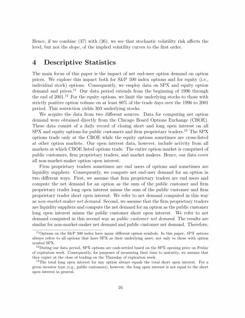
To illustrate the magnitude of the net demands, we compute approximate dailyprofits and losses (P&Ls) for the market makers’ hedged positions assuming daily delta-hedging. The daily and cumulative P&Ls are illustrated in Figure 5, which shows thatthe group of market makers faces substantial risk that cannot be delta-hedged, withdaily P&L varying between ca. $100M and $-100M. Further, the market makers makecumulative profits of ca. $800M over the 6-year period on their position taking.15 Withjust over a hundred SPX market makers on the CBOE, this corresponds to a profit ofapproxiamtely $1M per year per market maker. Hence, consistent with the premise of

15This number does not take into account the costs of market making or the profits from the bid-askspread on round-trip trades. A substantial part of market makers’ profit may come from the latter.

23

our model, market makers face substantial risk and are compensated on average forthe risk that they take.

01/04/96 12/18/97 12/08/99 12/31/01−150

−100

−50

0

50

100

150

P/L

($

1,0

00

,00

0s)

Daily Market Maker Profit/Loss

01/04/96 12/18/97 12/08/99 12/31/01−200

0

200

400

600

800

1000Cumulative Market Maker Profit/Loss

P/L

($

1,0

00

,00

0s)

Date

Figure 5: The top panel shows the market makers’ daily profits and losses (P&L)assuming they delta-hedge their option positions once per day. The bottom panelshows the corresponding cumulative P&Ls.

5 Empirical Results

Proposition 3 states that positive (negative) demand pressure on one option increases(decreases) the price of all options on the same underlying asset, while Proposition 4

24

states that demand pressure on low (high) strike options has a greater price impacton low (high) strike options. The empirical work in this section of the paper examinesthese two predictions of the model by investigating whether overall excess impliedvolatility is higher on trade dates where net demand for options is higher and whetherthe excess implied volatility skew is steeper on trade dates where the skew in the netdemand for options is steeper.

5.1 Excess Implied Volatility and Net Demand

We investigate first the time-series evidence for Proposition 3 by regressing a measureof excess implied volatility on one of various demand-based explanatory variables:

ExcessImplVol t = a + bDemandVar t + ǫt (38)

SPX:

We consider first this time-series relationship for SPX options, for which we defineExcessImplV ol as the average implied volatility of 1-month at-the-money SPX optionsminus the corresponding volatility of Bates (2005). When computing this variable, theSPX options included are those that have at least 25 contracts of trading volume,between 15 and 45 calendar days to expiration, and moneyness between 0.99 and 1.01.(We compute the excess implied volatility variable only from reasonably liquid optionsin order to make it less noisy in light of the fact that it is computed using only onetrade date.)16 By subtracting the volatility from the Bates (2005) model, we accountfor the direct effects of jumps, stochastic volatility, and the risk premium implied bythe equity market.

The independent variable, DemandV ar, is based on the aggregate net non-market-maker demand for SPX options that have 10–180 calendar days to expiration andmoneyness between 0.8 and 1.20. (Similar, in fact stronger, results obtain when public-customer demand is used instead.) We employ, separately, four different independentvariables. The first is simply the sum of all net demands. The other three indepen-dent variables correspond to “weighting” the net demands using the models based onthe market maker risks associated with, respectively, discrete trading, jumps in theunderlying, and stochastic volatility (Sections 3.1–3.3). Specifically, the net demandsare weighted by the Black-Scholes gamma in the discrete-hedging model, by kappacomputed using equally likely up and down moves of relative sizes 0.05 and 0.2 in thejump model, and by maturity-adjusted Black-Scholes vega in the stochastic volatilitymodel.

16By contrast, in the previous section of the paper, when implied volatility statistics were computedfrom less liquid options or options with more extreme moneyness or maturity, they were averaged overthe entire sample period.

25

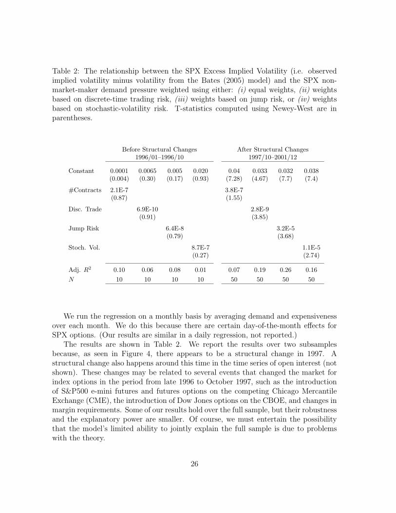
Table 2: The relationship between the SPX Excess Implied Volatility (i.e. observedimplied volatility minus volatility from the Bates (2005) model) and the SPX non-market-maker demand pressure weighted using either: (i) equal weights, (ii) weightsbased on discrete-time trading risk, (iii) weights based on jump risk, or (iv) weightsbased on stochastic-volatility risk. T-statistics computed using Newey-West are inparentheses.

Before Structural Changes After Structural Changes1996/01–1996/10 1997/10–2001/12

Constant 0.0001 0.0065 0.005 0.020 0.04 0.033 0.032 0.038(0.004) (0.30) (0.17) (0.93) (7.28) (4.67) (7.7) (7.4)

#Contracts 2.1E-7 3.8E-7(0.87) (1.55)

Disc. Trade 6.9E-10 2.8E-9(0.91) (3.85)

Jump Risk 6.4E-8 3.2E-5(0.79) (3.68)

Stoch. Vol. 8.7E-7 1.1E-5(0.27) (2.74)

Adj. R2 0.10 0.06 0.08 0.01 0.07 0.19 0.26 0.16

N 10 10 10 10 50 50 50 50

We run the regression on a monthly basis by averaging demand and expensivenessover each month. We do this because there are certain day-of-the-month effects forSPX options. (Our results are similar in a daily regression, not reported.)

The results are shown in Table 2. We report the results over two subsamplesbecause, as seen in Figure 4, there appears to be a structural change in 1997. Astructural change also happens around this time in the time series of open interest (notshown). These changes may be related to several events that changed the market forindex options in the period from late 1996 to October 1997, such as the introductionof S&P500 e-mini futures and futures options on the competing Chicago MercantileExchange (CME), the introduction of Dow Jones options on the CBOE, and changes inmargin requirements. Some of our results hold over the full sample, but their robustnessand the explanatory power are smaller. Of course, we must entertain the possibilitythat the model’s limited ability to jointly explain the full sample is due to problemswith the theory.

26

0 10 20 30 40 50 60 70 80−0.02

0

0.02

0.04

0.06

0.08

0.1

Exp

ensi

vene

ss

Month Number

ExpensivenessFitted values, early sampleFitted values, late sample

Figure 6: The solid line shows the expensiveness of SPX options, that is, impliedvolatility of 1-month at-the-money options minus the volatility measure of Bates (2005)which takes into account jumps, stochastic volatility, and the risk premium from theequity market. The dashed lines are, respectively, the fitted values of demand-basedexpensiveness using a model with underlying jumps, before and after certain structuralchanges (1996/01–1996/10 and 1997/10–2001/12).

We see that the estimate of the demand effect b is positive but insignificant overthe first subsample, and positive and statistically significant over the second longersubsample for all three model-based explanatory variables.17

The expensiveness and the fitted values from the jump model are plotted in Fig-ure 6, which clearly shows their comovement over the later sample. The fact that theb coefficient is positive indicates that, on average, when SPX net demand is higher(lower), excess SPX implied volatilities are also higher (lower). For the most successfulmodel, the one based on jumps, changing the dependent variable from its lowest to itshighest values over the late sub-sample would change the excess implied volatility byabout 5.6 percentage points. A one-standard-deviation change in the jump variable

17The model-based explanatory variables work better than just adding all contracts (#Contracts),because they give higher weight to near-the-money options. If we just count contracts using a morenarrow band of moneyness, then the #Contracts variable also becomes significant.

27

results in a one-half standard deviation change of excess implied volatility (the corre-sponding R2 is 26%). The model is also successful in explaining a significant proportionof the level of the excess implied volatility. Over the late subsample, the average levelis 4.9%, of which approximately one third – specifically, 1.7% – corresponds to theaverage level of demand, given the regression coefficient.

Further support for the hypothesis that the supply for options is upwardly slopingcomes from the comparison between the estimated supply-curve slopes following marketmaker losses, respectively gains. If market maker risk aversion plays an important rolein pricing options, then one would expect prices to be less sensitive to demand whenmarket makers are well funded – in particular, following profitable periods – thannot. This is exactly what we find. Breaking the daily sample18 in two subsamplesdepending on whether the hedged market maker profits over the previous 20 tradingdays is positive or negative,19 we estimate the regression (38) for each subsample andfind that, following losses, the b coefficient is approximately twice as large as thecoefficient obtained in the other subsample. For instance, in the jump model, theregression coefficient following losses is 2.6E-05 with a t-statistic 3.7 (330 observations),compared to a value of 1.1E-5 with t-statistic 6.1 in the complementary subsample (646observations).

Equity Options:

We consider next the time-series relationship between demand and expensiveness forequity options. In particular, we run the time-series regression (38) for each stock, andaverage the coefficients across stocks. The results are shown in Table 3. We considerseparately the subsample before and after the summer of 1999. This is because mostoptions were listed only on one exchange before the summer of 1999, but many werelisted on multiple exchanges after this summer. Hence, there was potentially a largertotal capacity for risk taking by market makers after the cross listing. See for instanceDe Fontnouvelle, Fishe, and Harris (2003) for a detailed discussion of this well-knownstructural break.

We run the time-series regression separately for the 303 underlying stocks withstrictly positive option volume on at least 80% of the trade days from the beginningof 1996 through the end of 2001. We compute the excess implied volatility as theaverage implied volatility of selected options,20 minus the GARCH(1,1) volatility, andnet demand as the total net non-market-maker demand for options with moneynessbetween 0.8 and 1.2 and maturity between 10 and 180 calendar days. We run theregression using monthly data on underlying stocks that have at least 12 months of

18Because of the structural changes discussed above, we restrict our attention to the period startingon October 1, 1997.

19Similar results obtain if the breaking point is the mean or median daily profit.20That is, options with moneyness between 0.95 and 1.05, maturity between 15 and 45 calendar

days, at least 5 contracts of trading volume, and implied volatilities available on OptionMetrics.

28

Table 3: The relationship between option expensiveness — i.e. implied volatility mi-nus GARCH volatility — and non-market-maker net demand for equity options on303 different underlying stock (Equation 38). We run time-series regressions for eachunderlying and report the average coefficients. The number p-val is the p-value of thebinomial test that the coefficients are equally likely to be positive and negative.

Before Cross-Listing of Options After Cross-Listing of Options04/1996–06/1999 10/1999–12/2001

Constant -0.01 0.02

NetDemand 12E-6 8.5E-6

Average Adj. R2 0.06 0.05

# positive 227 213

# negative 76 86

p-val 0.00 0.00

data available. (Daily regressions give stronger results.)The average coefficient b measuring the effect of demand on expensiveness is positive

and significant in both subsamples. This means that when the demand for equityoptions is larger their implied volatility is higher. The results are illustrated in Figure 7,which shows the expensiveness and fitted values of the demand effect on a monthlybasis. The positive correlation is apparent. We note that the relation between averagedemand and average expensiveness is more striking if we do a single, pooled regressionfor these variables. It is comforting, however, that the relation also holds when weconsider each stock separately.

Finally, we investigate the cross-sectional relationship between excess implied volatil-ity and net demand in the equity option market. We multiply the net demand variableby the price volatility of the underlying stock (defined as the sample return volatilityjust described multiplied by the day’s closing price of the stock.) We scale the netdemand in this way, because market makers are likely to be more concerned aboutholding net demand in their inventory when the underlying stock’s price volatility isgreater.

We run the cross-sectional regression on each day and then employ the Fama-MacBeth method to compute point estimates and standard errors. We also use theNewey-West procedure to control for serial-correlation in the slope estimates. Theslope coefficient is 5.9E-8 with a t-statistic of 6.44.

29

0 10 20 30 40 50 60 70 80−0.08

−0.06

−0.04

−0.02

0

0.02

0.04

0.06

Exp

ensi

vene

ss

Month Number

Expensiveness and Demand for Equity Options

ExpensivenessFitted values, early sampleFitted values, late sample

Figure 7: The solid line is the expensiveness of equity options, averaged across stocks.The dashed lines are, respectively, the fitted values of demand-based expensivenessbefore and after the cross-listing of options (1996/04–1999/05 and 1999/10–2001/12)using the average regression coefficients from stock-specific regressions and the averagedemand.

5.2 Implied Volatility Skew and Net Demand Skew

In order to investigate Proposition 4, we regress a measure of the steepness of theexcess implied volatility skew on one of two demand-based explanatory variables:

ExcessImplVolSkew t = a + bDemandVarSkew t + ǫt. (39)

SPX:

For the SPX analysis, ExcessImplVolSkew t is the date-t implied volatility skew overand above the skew predicted by the jumps and stochastic volatility of the underlyingindex. The implied volatility skew is defined as the average implied volatility of optionswith moneyness between 0.93 and 0.95 that trade at least 25 contracts on trade datet and have more than 15 and fewer than 45 calendar days to expiration, minus theaverage implied volatility of options with moneyness between 0.99 and 1.01 that meetthe same volume and maturity criteria. In order to eliminate the skew that is due

30

Table 4: The relationships between SPX implied-volatility skew and two potentialexplanatory variables: (i) the SPX non-market-maker demand skew and (ii) the jump-risk-model demand-based implied-volatility skew. T-statistics computed using Newey-West are in parentheses.

Before Structural Changes After Structural Changes1996/01–1996/10 1997/10–2001/12

Constant 0.032 0.04 0.04 0.032(57) (6.4) (20) (13.2)

#Contracts -1.2E-7 5.4E-7(-0.9) (3.4)

Jump Risk -3.0E-6 1.8E-5(-1.0) (3.0)

Adj. R2 0.08 0.14 0.22 0.28

N 10 10 50 50

to jumps and stochastic volatility of the underlying, we consider the implied volatilityskew net of the similarly defined volatility skew implied by the objective distribution ofBroadie, Chernov, and Johannes (2005) where the underlying volatility is that filteredfrom the Bates (2005) model.21

As explanatory variable, we use two measures. The first is the skew in net optiondemand, defined as the net non-market-maker demand for options with moneynessbetween 0.93 and 0.95 minus the net non-market-maker demand for options with mon-eyness between 0.99 and 1.01, using options with maturity between 10 and 180 calendardays. The second measure is the excess implied-volatility skew from the model with un-derlying jumps described in Section 3.2. (We do not consider the models with discretetrading and stochastic volatility since they do not have first-order skew implications asdescribed in Sections 3.1 and 3.3.)

Table 4 reports the monthly OLS estimates of the skewness regression and Figure 8illustrates the effects. As discussed in Section 5.1, we divide the sample into two sub-samples because of structural changes. The slope coefficient is significantly positive inthe late subsample using both the simple demand variable and the variable based onjump-risk.22 Using the jump-risk model, variation between the minimum and maxi-mum levels of the independent variable results in a skew change of about 3 percentage

21The model-implied skew is evaluated for one-month options with moneyness of, respectively, 0.94and 1. We thank Mikhail Chernov for providing this time series.

22The slope coefficient is also significant over the full sample; the demand skewness is less non-stationary than the level of demand over the full sample.

31

points. Further, a one standard deviation move in the independent variable results ina change in the dependent variable of 0.53 standard deviations.

0 10 20 30 40 50 60 70 800.01

0.02

0.03

0.04

0.05

0.06

0.07

0.08

Ske

w

Month Number

IV SkewFitted values, early sampleFitted values, late sample

Figure 8: The solid line shows the implied volatility skew for SPX options. The dashedlines are, respectively, the fitted values from the skew in demand before and aftercertain structural changes (1996/01–1996/10 and 1997/10–2001/12).

Equity Options:

We consider next the time-series relationship for equity options between skew indemand and skew in implied volatility. In particular, we run the time-series regression(39) for each stock, and average the coefficients across stocks.23 Once again, we con-sider separately the subsample before and after the summer of 1999, because of thewidespread move toward cross-listing in the summer of 1999.

The results are shown in Table 5. The time-series regression is run separately forthe same 303 underlying stocks as above. We compute the implied volatility skew asthe average implied volatility of selected low moneyness minus that of near-the-money

23Now the dependent variable is simply the time t implied volatility from low moneyness minusnear-the-money options.

32

Table 5: The relationship between implied volatility skew (i.e., implied volatility of lowmoneyness minus near-the-money options) and non-market-maker net demand skew(i.e., non-market-maker net demand for low moneyness minus high moneyness options)on 303 different underlying stocks (Equation 39). We run time-series regressions foreach underlying and report the average coefficients. The number p-val is the p-valuefrom the binomial test that the coefficients are equally likely to be positive and negative.

Before Cross-Listing of Options After Cross-Listing of Options04/1996–06/1999 10/1999–12/2001

Constant 0.03 0.03

NetDemand 4.0E-6 4.2E-6

Average Adj. R2 0.03 0.08

# positive 200 163

# negative 70 61

p-val 0.00 0.00

options.24 The skew in demand is the total net non-market-maker demand for optionswith moneyness between 0.80 and 1.00 minus that for options with moneyness between1.00 and 1.20.25 We run the regression using monthly data on underlying stocks thathave at least 12 months of data available.

The average coefficient b measuring the effect of skew in demand on skew in expen-siveness is positive and significant in both subsamples. This results implies that whenthe demand for equity options is more skewed their implied volatility is more skewed.

6 Conclusion

Relative to the Black-Scholes-Merton benchmark, index and equity options display anumber of robust pricing anomalies. A great deal of research has attempted to addressthese anomalies, in large part by generalizing the Black-Scholes-Merton assumptionsabout the dynamics of the underlying asset. While these efforts have met with somesuccess, non-trivial pricing puzzles remain. Further, it is not clear that this approachcan yield a satisfactory description of option prices. For example, index and equity op-

24That is, the average implied volatility from options with moneyness between 0.85 and 0.95 minusthe average implied volatility from option with moneyness between 0.97 and 1.03. These options musthave maturity between 15 and 45 calendar days, at least 1 contract of trading volume, and impliedvolatilities available on OptionMetrics.

25Options with maturity of 10 to 180 calendar day are included. The results are robust to variationin the definition in these demand categories.

33

tion prices display very different properties, although the dynamics of their underlyingassets are quite similar.

This paper takes a different approach to option pricing. We recognize that in con-trast to the Black-Scholes-Merton framework, in the real world options cannot be per-fectly hedged. Consequently, if intermediaries such as market makers and proprietarytraders who take the other side of end-user option demand are risk-averse, end-userdemand for options will impact option prices.

The theoretical part of the paper develops a model of competitive risk-averse inter-mediaries who cannot perfectly hedge their option positions. We compute equilibriumprices as a function of net end-user demand and show that demand for an option in-creases its price by an amount proportional to the variance of the unhedgeable part ofthe option and that it changes the prices of other options on the same underlying assetby an amount proportional to the covariance of their unhedgeable parts.

The empirical part of the paper measures the expensiveness of an option as itsBlack-Scholes implied volatility minus a proxy for the expected volatility over the lifeof the option. We show that on average index options are quite expensive by thismeasure, and that they have high positive end-user demand. Equity options, on theother hand, are on average slightly inexpensive and have a small negative end-userdemand. In accordance with the predictions of our theory, we find that options areoverall more expensive when there is more end-user demand for options and that theexpensiveness skew across moneyness is positively related to skew in end-user demandacross moneyness. Finally, demand effects are stronger following recent market makerlosses compared to times of recent market maker gains.

34

A Proofs

Proof of Lemma 1:

Note first that the boundedness of all the random variables considered (with the ex-ception of S) ensures that all expectations are finite.

The Bellman equation is

J(Wt; t,Xt) = −1

ke−k(Wt+Gt(dt,Xt))

= maxCt,qt,θt

−1

γe−γCt + ρEt [J(Wt+1; t + 1, Xt+1)]

(40)

Given the strict concavity of the utility function, the maximum is characterized bythe first-order conditions (FOC’s). Using the proposed functional form for the valuefunction, the FOC for Ct is

0 = e−γCt + kRfρEt [J(Wt+1; t + 1, Xt+1)] (41)

which together with (40) yields

0 = e−γCt + kRf

[

J(Wt; t,Xt) +1

γe−γCt

]

(42)

that is,

e−γCt = e−k(Wt+Gt(dt,Xt)) (43)

implying (4). The FOC’s for θt and qt are (5) and (6). We derive G recursively asfollows. First, we let G(t + 1, · ) be given. Then, θt and qt are given as the uniquesolutions to Equations (5) and (6). Clearly, θt and qt do not depend on the wealth Wt.Further, (42) implies that

0 = e−γCt − RfρEt

[

e−k(yt+1+(Wt−Ct)Rf+qt(pt+1−Rf pt)+θtRet+1+Gt+1(dt+1,Xt+1))

]

, (44)

that is,

e−γCt−krCt+krWt = RfρEt

[

e−k(yt+1+qt(pt+1−Rf pt)+θtRet+1+Gt+1(dt+1,Xt+1))

]

, (45)

which, using (4), yields the equation that defines Gt(dt, Xt) (since Xt is Markov):

e−krGt(dt,Xt) = RfρEt

[

e−k(yt+1+qt(pt+1−Rf pt)+θtRet+1+Gt+1(dt+1,Xt+1))

]

(46)

35

At t = T , we want to show the existence of a stationary solution. First note thatthe operator A defined by

AF (w; x) = maxC,θ

−1

γe−γC + ρEt [F (Wt+1, Xt+1)|Wt = w,Xt = x]

subject toWt+1 = yt+1 + (Wt − C)Rf + θRe

t+1,

satisfies the conditions of Blackwell’s Theorem,26 and is therefore a contraction.Furthermore, A maps any function of the type

F (w; x) = −1

ke−kwg(x)

into a function of the same type, implying that the restriction of A to g, denoted alsoby A, is a contraction as well.

We now show that there exists m > 0 such that A maps the set

Gm = g : X → R : g is continuous, g ≥ m

into itself.Continuity holds by assumption (the Feller property). Let us look for m > 0. Since

Ag ≥ infx

infθ

RfρE[

e−k(yt+1+θRet+1)g(Xt+1)

1

Rf |Xt = x]

≥ infx

infθ

RfρE[

e−k(yt+1+θRet+1)|Xt = x

] (

minz

g(z))

1

Rf

≥ B(

minz

g(z))

1

Rf

for a constant B > 0 (the inner infimum is a strictly positive, continuous function of

x ∈ X compact), showing that the assertion for any m not bigger than BRf

Rf−1 .Since Gm is complete, we conclude that A has a (unique) fixed point in Gm (which,

therefore, is not 0).It remains to prove that, given our candidate consumption and investment policy,

limt→∞

E[

ρ−te−kWt]

= 0.

Start by noting that, for t > T ,

Wt+1 = Wt − (Rf − 1)G(Xt) + yt+1 + θtRet+1,

26See, for instance, Stokey, Lucas, and Prescott (1989).

36

implying, by a repeated application of the iterated expectations, that

ET

[

e−k(Wt+G(Xt))]

= e−k(WT +G(XT )),

which is bounded. Since G(Xt) is bounded, it follows that limt→∞ E[

ρ−te−kWt]

= 0.The verification argument is standard, and particularly easy in this case given the

boundedness of g.

Proof of Proposition 1:

Given a position process from date t onwards and a price process from date t + 1onward, the price at time t is determined by (6). It is immediate that pt is measurablewith respect to time-t information.

Proof of Proposition 2:

Part (i) is immediate, since prices are linear. Part (ii) follows because, for any a ∈ R,the pricing kernel is kept exactly the same by the offsetting change in (q, θ).

Proof of Proposition 3:

Part a) is immediately since a variance is always positive. The proof of b) is based onthe following result.

Lemma 2 Given h1 and h2 convex functions on R, ∀β < 0, α, γ ∈ R, ∃α′, γ′ ∈ R suchthat

|h1(x) − α′x − γ′| ≤ |h1(x) − αx − βh2(x) − γ|

∀x ∈ R. Consequently, under any distribution, regressing h1 on h2 and the identityfunction results in a positive coefficient on h2.

Letting pt+1 = pt+1 − Edt [pt+1] and suppressing subscripts, consider the expression

Ψ = Ed[

pipj]

Var(Re) − Ed[

piRe]

Ed[

pjRe]

,

which we want to show to be positive. Letting pi = Ed[pi|S] and pj = Ed[pj|S], wewrite

Ψ = Ed[

Cov(

pi, pj|S)

Var(Re) + pipjVar(Re) − Ed[

piRe]

Ed[

pjRe]]

= Ed[

Cov(

pi, pj|S)

Var(Re)]

+ Ed[

pipjVar(Re) − Ed[

piRe]

Ed[

pjRe]]

.

The first term is positive by assumption, while the second is positive because pi andpj are convex and then using Lemma 2 .

37

Proof of Lemma 2: We consider three cases: (i) the intersection of the graphs ofh1 and g ≡ γ + αId + βh2 is empty; (ii) their intersection is a singleton; (iii) theirintersection contains more than one point.

(i) Since the graphs do not intersect, there exists a hyperplane that separates theconvex sets (x, y) : h1(x) ≤ y and (x, y) : g(x) ≥ y.

(ii) The same is true if the two graphs have a tangency point. If they intersectin one point, x, and are not tangent, then assume that, for x < x, h1(x) > g(x)(a similar argument settles the complementary case). The convex set generated by(x, h1(x) ∨ (x, (h1(x)) : x < x ∨ (x, g(x)) : x > x) and the one generated by(x, h1(x) ∨ (x, (h1(x)) : x > x ∨ (x, g(x)) : x < x) have only one point incommon, and therefore can be separated with a hyperplane.

(iii) Consider the line generated by the intersection. If there existed a point x atwhich the ordinate of the line was higher than h1(x) and than g(x), then it would followthat at least one of the intersection points is actually interior to (x, y) : h1(x) ≤ y,which would be a contradiction. Similarly if the line was too low.

Proof of Theorem 3:

We compute the sensitivity of current prices to a deviation in future positions from 0in the direction of demand ds = ǫsds at time s by differentiating with respect to ǫs = ǫ(evaluated at ǫ = 0). We then aggregate the demands at all times to compute the totaleffect:

∂pt

∂ǫ=

∑

s≥0

∂pt

∂ǫs

∂ǫs

∂ǫ=∑

s≥0

∂pt

∂ǫs

To compute the price effect of expected demand at any time s, we note that it followsfrom the dealer’s problem that

pt = Et

[

ρs−te−γ(Cs−Ct)ps

]

which implies

∂pt

∂ǫs

= Et

[

ρs−te−γ(Cs−Ct)∂ps

∂ǫs

]

= R−(s−t)f E∗

t

[

∂ps

∂ǫs

]

= R−(s−t)f E∗

t

[

∂ps

∂qjs

qjs

]

.

38

where we use that ∂Ct

∂ǫs= ∂Cs

∂ǫs= 0 at q = 0. The equality ∂Cs

∂ǫs= 0 follows from

∂Cs

∂qjs

=k

γ

∂G(s,Xs; q)

∂qjs

= −k2Rfρ

γE∗

s

[

pjs+1 − Rfp

js +

∂θs

∂qjs

Res+1

]

= 0 (47)

and the other equality follows from differentiating the condition that marginal rates ofsubstitution are equal

e−γCt = e−ρ(s−t)Et

[

e−γCs]

,

which gives that

e−γCt∂Ct

∂ǫs

= e−ρ(s−t)Eu

[

e−γCs∂Cs

∂ǫs

]

= 0

It remains to show that the price is a smooth (C∞) function of ǫ. Consider aprocess dt characterized by dt = 0 for all t > T , and let the demand process be givenby dt = ǫtdt = −qt. At time t, the following optimality conditions must hold:

e−γCt = (Rfρ)T+1−t Et

[

e−k(WT+1+GT+1)]

(48)

0 = Et

[

e−k(WT+1+GT+1)Ret+1

]

(49)

0 = Et

[

e−k(WT+1+GT+1)(

pT+1 − RT+1−tf pt

)]

, (50)

with

WT+1 = (Wt−Ct)RT+1−tf +

T∑

s=t

(

ys+1 − Cs+1 + θsRes+1 − ǫsds (ps+1 − Rfps)

)

RT+1−sf +yT+1.

We use the notation pT+1 for the time T+1-money value of the payoff of options expiredby T + 1.

We show by induction that, given Xs, (ps, θs, Cs) is a smooth function of (ǫs, . . . , ǫs+1).Note that the statement holds trivially for s > T .

Assume therefore the statement for all s > t. There are nt+2 equations in (48)–(50),with nt+1 being the number of derivatives priced at time t. Note that the equationsdo not depend on ǫs for s < t and that they are smooth in ǫs for all s , as well as inθt, Ct, and pt. In order to prove the claim, we have to show that the derivative of thefunctions giving (48)–(50) with respect to (pt, θt, Ct) is invertible (at ǫ = 0 suffices), i.e.,it has non-zero determinant. The implicit function theorem, then, proves the inductionstatement for s = t.

39

The non-zero determinant is shown as follows. If we let FC , Fθ, respectively Fq

denote the functions implicit in equations (48)–(50), it follows easily that

DCFC 6= 0

DCFθ = 0

DCFq = 0

DθFθ 6= 0

DpFθ = 0

det(DpFq) 6= 0,

implying that D(Ct,θt,pt)F has non-zero determinant.

Proof of Proposition 4:

Consider an optimally hedged short put position with strike price K < RfSt. Withx = St+1 − RfSt, the payoff from this position is

Π(x) = −d(K − RfSt − x)+ + θx.

The optimality of the hedge means that, under the risk-neutral measure,

Ed[

e−kΠ(x)x]

= 0.

Note that, since K < RfSt, Π(x) < 0 for x > 0 and Π(x) > 0 for K−RfSt < x < 0.Consequently, given the symmetry of x around 0 and the zero-expectation conditionabove, with ξ denoting the density of x,

∫ ∞

K

(

e−kΠ(x)x − e−kΠ(−x)x)

ξ(x) dx = −

∫ K

0

(

e−kΠ(x)x − e−kΠ(−x)x)

ξ(x) dx < 0.

It immediately follows that it cannot be true that Π(−x) ≥ Π(x) for all x > |K−RfSt|.In other words, for some value x > |K − RfSt|, Π(−x) < Π(x), which then givesd + θ > −θ, or |θ| < 1

2|d|: the payoff is more sensitive to large downward movements

in the underlying than to large upward movements. Thus, there exists K such that,for all St+1 < K,

Π(St+1 − RfSt) < Π(−(St+1 − RfSt)),

implying that, whenever K ′ < K and K ′′ = 2RfSt − K ′,

p(p,K ′, d) > p(c,K ′′, d)

p(p,K ′, 0) = p(c,K ′′, 0),

the second relation being the result of symmetry.

40

Arbitrary Number of Time Units ∆t between Hedging Dates:

Most of our analysis relies on the assumption that there is 1 time unit per period(which simplifies notation). For the results on frequent hedging (i.e. ∆t → 0) inPropositions 5 -7, it is useful to see how to adapt the results for an arbitrary ∆t.

For simplicity, let the stock price be S = X1, with no dividends, and let X followa jump-diffusion with time-independent coefficient functions:

dXt = (µ(Xt) dt + v(Xt) dBt + η(Xt)dNt) , (51)

where Nt is a counting process with arrival intensity λ(Xt) and where the jumps sizeis drawn from a uniformly bounded distribution also depending on Xt.

Let ∆t be arbitrary, provided that all derivatives mature at times that are integralmultiples of ∆t. The dealer’s problem is to maximize

U(Ct, Ct+∆t, . . .) = Et

[

∞∑

l=0

ρl∆tu (Ct+l∆t) ∆t

]

,

with u(c) = − 1γe−γc. At any time t, the dealer must choose the consumption level

Ct, the dollar investment θt in the underlying, and the number of derivatives heldqt = (qi

t)i∈It, while satisfying the transversality condition limt→∞ E

[

ρ−te−kWt]

= 0,where the dealer’s wealth evolves as

Wt+∆t= (Yt+∆t

− Yt) + (Wt − Ct∆t)Rf + qt(pt+∆t− rpt) + θtR

et+∆t

. (52)

Here, Yt =∫ t

0ysds represents the cumulative endowment, and C is the annualized

consumption.The results of Lemma 1 become

J(Wt; t,Xt) = −1

ke−k(Wt+Gt(dt,Xt)) (53)

Ct =k

γ(Wt + Gt(dt, Xt)) , (54)

with k =Rf−1

Rf∆tγ = er∆t−1

er∆t∆tγ. The stock and derivative holdings are characterized by the

first-order conditions

0 = Et

[

e−k(Yt+∆t+θtRe

t+∆t+qt(pt+∆t

−rpt)+Gt+∆t(dt+∆t

,Xt+∆t))Re

t+∆t

]

(55)

0 = Et

[

e−k(yt+∆t+θtRe

t+∆t+qt(pt+∆t

−rpt)+Gt+∆t(dt+∆t

,Xt+∆t)) (pt+∆t

− rpt)]

, (56)

where, for t ≤ T , the function Gt(dt, Xt) is derived recursively using (55), (56), and

e−kRf Gt(dt,Xt) = RfρEt

[

e−k(yt+∆t+qt(pt+∆t

−rpt)+θtRet+∆t

+Gt+∆t(dt+∆t

,Xt+∆t))]

, (57)

41

and, for t > T , the function Gt(dt, Xt) = G(Xt) where (G(Xt), θ(Xt)) solves

e−kRf G(Xt) = RfρEt

[

e−k(yt+∆t+θtRe

t+∆t+G(Xt+∆t

))]

(58)

0 = Et

[

e−k(yt+∆t+θtRe

t+∆t+G(Xt+∆t

))Ret+∆t

]

. (59)

Replicating calculations in the body of the paper, with the obvious modification,the statement of Theorem 3 is generalized to

pt = pt(0) + γRf − 1

∆t

[

E0t

(

pt+∆tp′t+∆t

)

dt +∑

l>0

e−rl∆tE0t

(

pt+(l+1)∆tp′t+(l+1)∆t

dt+l∆t

)

]

ǫ

+ O(ǫ2).

Proofs of Propositions 5 -7:

In order to prove Propositions 5 -7, we proceed with a few technical preliminaries. Weassume that under the risk-neutral pricing measure given by d = 0 the process Xt

is a jump-diffusion of the same functional form as given by Equation (51). For zerodemand, an option price is defined by

p(St, t; X(1)t ) = e−r(T−t)E0

[

(ST − K)+ |Xt

]

,

regardless of the frequency of trading, where X(1) = (X2, . . . , Xn).For the computation of the covariances necessary, we shall be relying on applications

of the following result. For sufficiently smooth functions g, h : Rn → R,

d(g(Xt, t)h(Xt, t)) = mght dt + dM gh

t ,

where M gh is a martingale and

mght =

(

gXµ + gt +1

2tr(

gXXvv⊤)

)

h +

(

hXµ + ht +1

2tr(

hXXvv⊤)

)

g +

gXvv⊤h⊤X − λ

(

E0t [g(Xt + η)h(Xt + η)] − g(Xt)h(Xt)

)

.

It follows that

E0t [g(Xt+∆t

, t + ∆t)h(Xt+∆t, t + ∆t)] = g(Xt, t)h(Xt, t) + mgh

t ∆t + O(∆2t ). (60)

We now apply this approximation result to compute the unhedgeable price covari-ances. We start with the hedge ratio θ, which requires estimating

E0t

[

pt+∆tRe

t+∆t

]

=1

St

(

v1.v⊤p⊤X + λpE0t [η] − λ

(

E0t [p(Xt + η)η]

))

∆t + O(∆2t )

=1

St

(

v1.v⊤p⊤X − λ(

E0t [(p(Xt + η) − p(Xt)) η]

))

∆t + O(∆2t )

42

and

E0t

[

(

Ret+∆t

)2]

=1

S2t

(

v1.(v1.)⊤ − λE0[

η2])

∆t + O(∆2t ),

where v1. denotes the first row of the matrix v. This gives θ up to order O(∆t).Finally, compute the un-hedged payoff covariance using θ and applying (60) with

appropriate choices for g and h:

Cov0t

[

pit+∆t

, pjt+∆t

]

=(

mpipj

t − θitm

pjRe

t − θjtm

piRe

t + θitθ

jtm

(Re)2

t

)

∆t + O(∆2t ),

where the only quantity not computed above is

mpipj

t = 2rpipj + pjXv(pi

Xv)⊤ − λE0t

[(

pi(Xt + η) − pi(Xt)) (

pj(Xt + η) − pj(Xt))]

Here we used the fact that, since e−rsp(Xs, s) is a martingale, the fundamental pricingPDE holds, i.e., the drift of p(Xs, s) equals rp(Xs, s).

We now specialize the model to three choices, corresponding to each of Sections 3.1–3.3:

Proof of Proposition 5:

In the first model S = X1 is a Markov diffusion, i.e., the jump component is 0. Weobtain immediately that θt = StpS(St, t) + O(∆t) = StfS(St, t) + O(∆t), and thereforeCov0

t

[

pit+∆t

pjt+∆t

]

= 0 up to terms in O(∆2t ).

To obtain a more nuanced answer we work directly with an exact third-order Taylorexpansion of the function p(St+∆t

, t + ∆t) around the point (St, t). It follows that

Cov0t

[

pit+∆t

, pjt+∆t

]

= Cov0t

[

1

2f i

SS∆S2 + ∆S O(∆t) + O(∆2t ),

1

2f j

SS∆S2 + ∆S O(∆t) + O(∆2t )

]

=1

4f i

SSf jSSVar0

t

[

∆S2]

+ O(

∆5

2

t

)

=1

2f i

SSf jSSv4∆2

t + O(

∆5

2

t

)

.

Proof of Proposition 6:

In this model, S is a Markov jump-diffusion. Let η = S−1η be the relative jump sizeand σ = S−1v be the relative volatility, giving

θt =σ2fSSt − λE0

t [(p(St(1 + η)) − p(St)) η]

σ2 − λE0[η2]+ O(∆t)

43

and

Cov0t

[

pit+∆t

, pjt+∆t

]

=(

(f iSSt − θi)(f j

SSt − θj)σ2 + λE0t

(

κiκj))

∆t + O(∆2t ),

with κi = f i(St(1 + η)) − f i − θiη.

Proof of Proposition 7:

Here we let X = (S, σ)⊤ with

dSt = rSt dt + σtSt dB1,t

dσt = φ(σ − σt) dt + σσ(St, σt) dB2,t.

Since the Brownian motion driving the volatility, B2,t is independent from the onedriving the underlying return, B1,t, the hedge ratio is the same as in the 1-dimensionalMarkov-diffusion case,

θt = fSSt + O(∆t),

and

Cov0t

[

pit+∆t

, pjt+∆t

]

= f iσf

jσσ2

σ∆t + O(∆2t ),

where fσ is the derivative of f with respect to the second argument.

Empirical Implementation:

For the empirical implementation of the model, we do as follows. We weight thedemand of the included options according to the model-implied covariances of un-hedgeable parts, using the models of Sections 3.1–3.3. Specifically, for the diffusiverisk we compute an option’s Black-Scholes-Merton gamma (i.e. the second derivativewith respect to the price of the underlying) evaluated at the option’s moneyness andmaturity, 20% volatility, S = 1, an interest rate of r = 5%, dividend rate q = 1.5%,∆t = 0.01. The results are robust the choices of these parameters. We keep S, r, q,and σ constant throughout the sample to avoid biases arising from changes of thesevariables. Hence, changes in the model-implied demand effect is solely due to changesin demand patterns.

Similarly, we compute the demand effect with stochastic volatility risk by comput-ing the Black-Scholes-Merton vega (i.e. the derivative with respect to the volatility)evaluated at the same parameters as above and adjusting for maturity. We use thematurity adjustment described in Equation 37, where the volatility mean-reversionparameter φ is set to 6 based on the estimate of Pan (2002).

We compute the covariance jump risk E(κiκj) by computing for each option itsunhedged profit/loss in the case of equally likely jumps of 5% and -20%, jump arrival

44

rate of 5% per year, and the parameters above. For this, we compute a jump-adjustedoption price function f without demand effects and without jump risk premia using astraightforward adaptation of Merton (1976) We use the delta hedging given by θ = fS.Finally, we compute the variables κ and their covariance using the definitions (32) and(34).

45

References

Amin, K., J. D. Coval, and H. N. Seyhun (2004): “Index Option Prices and StockMarket Momentum,” Journal of Business, 77.

Bakshi, G., N. Kapadia, and D. Madan (2003): “Stock Return Characteristics,Skew Laws, and the Differential Pricing of Individual Equity Options,” Review ofFinancial Studies, 16(1), 101–143.

Bates, D. S. (2000): “Post ’87 Crash Fears in the S&P 500 Futures Options Market,”Journal of Econometrics, 94, 181–238.

(2003): “Empirical Option Pricing: A Retrospection,” Journal of Economet-rics, 116, 387–404.

(2005): “Maximum Likelihood Estimation of Latent Affine Processes,” Reviewof Financial Studies, forthcoming.

Bernardo, A. E., and O. Ledoit (2000): “Gain, Loss and Asset Pricing,” TheJournal of Political Economy, 108(1), 144–172.

Black, F., and M. S. Scholes (1973): “The Pricing of Options and CorporateLiabilities,” The Journal of Political Economy, 81, 637–654.

Bollen, N. P., and R. E. Whaley (2004): “Does Net Buying Pressure Affect theShape of Implied Volatility Functions?,” Journal of Finance, 59, 711–753.

Bondarenko, O. (2003): “Why are Put Options So Expensive?,” working paper,University of Illinois at Chicago.

Brennan, M. (1979): “The Pricing of Contingent Claims in Discrete Time Models,”Journal of Finance, 34(1), 53–68.

Broadie, M., M. Chernov, and M. Johannes (2005): “Model Specification andRisk Premia: Evidence from Futures Options,” Working Paper, Columbia.

Cochrane, J. H., and J. Saa-Requejo (2000): “Beyond Arbitrage: Good-DealAsset Price Bounds in Incomplete Markets,” The Journal of Political Economy,108(1), 79–119.

Constantinides, G. M., J. C. Jackwerth, and S. Perrakis (2005): “Mispricingof S&P 500 Index Options,” Working Paper, University of Chicago.

Constantinides, G. M., and S. Perrakis (2002): “Stochastic dominance boundson derivatives prices in a multiperiod economy with proportional transaction costs,”Journal of Economic Dynamics and Control, 26, 1323–1352.

46

Coval, J. D., and T. Shumway (2001): “Expected Option Returns,” Journal ofFinance, 56(3), 983–1009.

De Fontnouvelle, P., R. P. H. Fishe, and J. H. Harris (2003): “The Behaviorof Bid-Ask Spreads and Volume in Options Markets during the Competition forListings in 1999,” Journal of Finance, 58(6), 2437–2463.

de Roon, F., T. E. Nijman, and C. Veld (2000): “Hedging Pressure Effects inFutures Markets,” Journal of Finance, 55(3), 1437–1456.

Driessen, J., and P. Maenhout (2003): “A Portfolio Perspective on Option PricingAnomalies,” Working Paper, University of Amsterdam.

Figlewski, S. (1989): “Options Arbitrage in Imperfect Markets,” Journal of Finance,44(5), 1289–1311.

Gabaix, X., A. Krishnamurthy, and O. Vigneron (2004): “Limits of Arbitrage:Theory and Evidence from the Mortgage-Backed Securities Market,” Working Paper,MIT.

Greenwood, R. (2005): “Short-and long-term demand curves for stocks: theory andevidence on the dynamics of arbitrage,” Journal of Financial Economics, fortcoming.

Hakansson, N. (1979): “The Fantastic World of Finance: Progress and the FreeLunch,” The Journal of Financial and Quantitative Analysis, 14, 717–734.

Hicks, J. R. (1939): Value and Capital. Cambridge: Oxford University Press.

Hugonnier, J., D. Kramkov, and W. Schachermayer (2005): “On UtilityBased Pricing of Contingent Claims in Incomplete Markets,” Mathematical Finance,15(2), 203–212.

Jackwerth, J. (2000): “Recovering risk aversion from option prices and realizedreturns,” Review of Financial Studies, 13, 433–451.

Keynes, J. M. (1923): “Some Aspects of Commodity Markets,” Manchester GuardianCommercial, European Reconstruction Series, Section 13, 784–786.

Longstaff, F. A. (1995): “Option Pricing and the Martingale Restriction,” Reviewof Financial Studies, 8(4), 1091–1124.

Merton, R. (1973): “The Theory of Rational Option Pricing,” Bell Journal of Eco-nomics and Management Science, 4, 141–183.

(1976): “Option Pricing when the Underlying Stock Returns are Discontinu-ous,” Journal of Financial Economics, 5, 125–144.

47

Newman, Y., and M. Rierson (2004): “Illiquidity Spillovers: Theory and Evidencefrom European Telecom Bond Issuance,” Working Paper, Stanford Graduate Schoolof Business.

Pan, J. (2002): “The Jump-Risk Premia Implicit in Options: Evidence from an Inte-grated Time-Series Study,” Journal of Financial Economics, 63, 3–50.

Poteshman, A. M. (2001): “Underreaction, Overreaction, and Increasing Misreac-tion to Information in the Options Market,” Journal of Finance, 56(3), 851–876.

Rubinstein, M. (1976): “The Valuation of Uncertain Income Streams and Pricing ofOptions,” Bell Journal of Economics, 7, 407–425.

Shleifer, A., and R. W. Vishny (1997): “The Limits of Arbitrage,” Journal ofFinance, 52(1), 35–55.

Soner, H. M., S. E. Shreve, and J. Cvitanic (1995): “There is No NontrivialHedging Portfolio for Option Pricing with Transaction Costs,” The Annals of AppliedProbability, 5(2), 327–355.

Stapleton, R. C., and M. G. Subrahmanyam (1984): “The Valuation of Mul-tivariate Contingent Claims in Discrete Time Models,” Journal of Finance, 39(1),207–228.

Stein, J. (1989): “Overreactions in the Options Market,” Journal of Finance, 44,1011–1023.

Stokey, N. L., R. E. Lucas, and E. C. Prescott (1989): Recursive Methods inEconomic Dynamics. Harvard University Press.

Wurgler, J., and E. V. Zhuravskaya (2002): “Does Arbitrage Flatten DemandCurves for Stocks?,” Journal of Business, 75(4), 583–608.

48