NBER WORKING PAPER SERIES

GLOBAL PRODUCTION WITH EXPORT PLATFORMS

Felix Tintelnot

Working Paper 22236http://www.nber.org/papers/w22236

NATIONAL BUREAU OF ECONOMIC RESEARCH1050 Massachusetts Avenue

Cambridge, MA 02138May 2016

I am grateful to my advisors Jonathan Eaton and Stephen Yeaple for their guidance, encouragement, and support. I am also grateful to Andrés Rodríguez-Clare and Paul Grieco for encouragement and various discussions on the topic. I wish to thank the editor, Elhanan Helpman, and three anonymous referees for their comments and suggestions. I thank Pol Antras, Costas Arkolakis, Kerem Cosar, Anca Cristea, Teresa Fort, Anna Gumpert, Christian Gourieroux, Oleg Itskhoki, David Jinkins, Corinne Jones, Sung Jae Jun, Konstantin Kucheryavyy, Matthias Lux, Kalina Manova, Eduardo Morales, Andreas Moxnes, Joris Pinkse, Natalia Ramondo and seminar participants at Arizona State University, Boston University, University of Chicago, University of British Columbia, MIT, University of Michigan, NBER Summer Institute, Pennsylvania State University, Stanford University, University of Wisconsin, and Yale University for helpful comments and suggestions. I thank the German Bundesbank for the hospitality and access to its Microdatabase Direct investment (MiDi). This paper is part of my PhD dissertation at Penn State. I continued working on this project while visiting the International Economics Section at Princeton University, whom I thank for their hospitality. Meru Bhanot, Ken Kikkawa, and Zhida Gui provided outstanding research assistance. This work was completed in part with resources provided by the University of Chicago Research Computing Center. I gratefully acknowledge the support of the National Science Foundation (under grant SES-1459950) and the Andrew and Betsy Rosenfield Program in Economics, Public Policy, and Law at the Becker Friedman Institute. The views expressed herein are those of the author and do not necessarily reflect the views of the National Bureau of Economic Research.

NBER working papers are circulated for discussion and comment purposes. They have not been peer-reviewed or been subject to the review by the NBER Board of Directors that accompanies official NBER publications.

© 2016 by Felix Tintelnot. All rights reserved. Short sections of text, not to exceed two paragraphs, may be quoted without explicit permission provided that full credit, including © notice, is given to the source.

Global Production with Export PlatformsFelix TintelnotNBER Working Paper No. 22236May 2016JEL No. F12,F23,L23

ABSTRACT

Most international commerce is carried out by multinational firms, which use their foreign affiliates both to serve the market of the host country and to export to other markets outside the host country. In this paper, I examine the determinants of multinational firms' location and production decisions and the welfare implications of multinational production. The few existing quantitative general equilibrium models that incorporate multinational firms achieve tractability by assuming away export platforms – i.e. they do not allow foreign affiliates of multinationals to export – or by ignoring fixed costs associated with foreign investment. I develop a quantifiable multi-country general equilibrium model, which tractably handles multinational firms that engage in export platform sales and that face fixed costs of foreign investment. I first estimate the model using German firm-level data to uncover the size and nature of costs of multinational enterprise and show that the fixed costs of foreign investment are large. Second, I calibrate the model to data on trade and multinational production for twelve European and North American countries. Counterfactual analysis reveals that multinationals play an important role in transmitting technological improvements to foreign countries and that the pending Canada-EU trade and investment agreement could divert a sizable fraction of the production of EU multinationals from the US to Canada.

Felix TintelnotDepartment of EconomicsUniversity of Chicago5757 South University AvenueChicago, IL 60637and NBERtintelnot@uchicago.edu

1 Introduction

Multinational firms account for a large share of global output and employment.1 In structuring their global

operations, these firms confront various costs of multinational production and trade. For instance, whether a

firm should pursue a strategy of maintaining many plants to avoid shipping costs or a strategy of consolidating

production in a few locations turns on the size of the fixed costs of establishing foreign plants relative to the

costs of shipping goods. Further, given a set of production locations, the choice of which product to produce

where depends on the interaction of comparative advantage and the cost of shipping goods. In the data, firms

tend to concentrate their production in only a few locations, which is intuitive under increasing returns at

the plant level, and to use export platform sales in order to serve markets outside the host country. For US

multinationals’ affiliates in Europe, Figure 1 documents the proportion of output exported to other countries

from the host country. Across all countries (including countries outside Europe), export platform sales account

for an average of 43 percent of multinationals’ foreign output, a share that is systematically higher for smaller

countries.

In this paper, I develop a framework that is designed to answer several key questions. First, what are

the costs associated with multinational production? How important are the fixed costs of establishing foreign

operations relative to possible efficiency losses due to remote management? Second, how does the process of

globalization, measured as a fall in these costs, affect the structure of global production? Will globalization

result in firms’ consolidating production in a few favored locations, or will firms expand their global production

networks? Third, how does allowing for multinational production affect our understanding of the welfare effects

in a general equilibrium trade model?

Export platform sales, together with the presence of fixed cost of establishing foreign plants, imply a

hard permutation problem for deciding on how to structure a firm’s global operations. A firm simultaneously

needs to decide the set of countries in which to establish a production plant, which markets to serve from each

plant, and how much to sell to each market. Perhaps for this reason, the literature on multinational firms in

multi-country settings has made extreme assumptions. Existing work either does not allow for export platform

sales or ignores the fixed costs of establishing foreign plants. The key idea for tractability in the framework

presented in this paper is to consider a firm as consisting of a continuum of products and to treat a firm’s

product-location-specific productivities as random variables, similarly to how Eaton and Kortum (2002) treat

a country’s productivities. By allowing each firm to produce a continuum of products, I smooth out the firm’s

1A multinational firm is a company with enterprises in more than one country. I define its home country as the country inwhich the parent company of the enterprises is registered. Usually, this coincides with the country of the multinational firm’sheadquarters. According to Bernard, Jensen, and Schott (2009), in the year 2000 multinational firms accounted for nearly 80percent of US imports and exports, and employed 18 percent of the entire US civilian workforce. Publicly available BEA datashows that, in the manufacturing sector, the sales by US MNEs’ majority-owned foreign affiliates are more than twice as large asaggregate US exports.

2

Figure 1: Export platform shares for US multinationals in Europe

Notes: This figure displays the share of output that is exported to countries outside the host country by USmultinationals’ majority-owned foreign affiliates in the manufacturing sector. For the European countries displayedin the figure, typically only about 5 percent of the output is sold back to the US. An exception is Ireland, for which17 percent of the output is sold to the US. Across all countries (including countries outside Europe), US-ownedforeign affiliates in the manufacturing sector sell 43 percent of their output to countries outside the host country –13 percent of the output is sold to the US and 30 percent to other foreign countries. The statistics are for the year2004. Source: BEA.

response to changes in aggregate variables and obtain intuitive, closed-form expressions for the output at each of

the firm’s plants. A firm’s output is a function of the locations of its plants, the productivity of each plant, the

input costs in the plants’ host countries, and the market potential of the plants’ host countries. Furthermore,

the model delivers a probability with which a firm chooses a set of plants, as the fixed cost to establish a plant

in a foreign country is stochastic and firm-country-specific.

With this framework, I conduct a two-tiered empirical analysis. Using German firm-level data on output

at the parent and affiliate levels, I estimate both the variable production costs in foreign countries as well as the

distribution of fixed costs to establish a foreign plant. I find that German multinational firms face between 5

percent (Austria) and 35 percent (United States) larger variable production costs abroad than at home and face

substantial fixed costs of establishing foreign affiliates. I also document that multinational firms tend to produce

3

a large share of their output domestically and that this pattern is robust across size cohorts and industries.

In the second tier of my empirical inquiry, I focus on general equilibrium welfare analysis. I calibrate

the general equilibrium outcomes of the model to match data on bilateral trade flows, bilateral shares of foreign

production, and the country-specific production cost estimates from German multinational firms. The cost

estimates of German multinationals enable me to include both variable foreign production frictions and fixed

costs in the analysis that otherwise includes only aggregate data. I solve for the endogenous relative wages and

price indices in every country. With the calibrated model, I explore how globalization changes the structure of

global production. For example, currently, Canada and the EU are in the ratification process of a trade and

investment agreement: CETA. If one supposes that the agreement is signed and yields a 20 percent reduction

of variable and fixed production costs between the signatories, then – according to my calibrated model – EU

multinationals would divert around five percent of their production from the US to Canada. These findings

hinge on the possibility of export platform sales from Canada to the US. Without this possibility, the location

and output decisions of European firms are independent between Canada and the United States. Instead, I

find that a Canada-EU trade and investment agreement could induce a strong third-party effect on the United

States.

Furthermore, I demonstrate that a more complete model of multinational production and trade can

revise answers to classic questions in the trade literature. Specifically, I investigate how technology shocks in

one country affect production and welfare outcomes in all countries, a question often studied in trade models

without multinational production. Multinational production provides an additional channel through which

technology can flow across countries. Suppose all US firms improve their technology by 20 percent. I find

that the welfare gains in foreign countries from such a technology improvement are an order of magnitude

larger when multinational production is taken into account. The magnitude of the gains in foreign countries

depends crucially on the cost of foreign production, which I carefully estimate in this paper. In models without

multinational production, the cost of foreign production is infinite by assumption.

The model presented in this paper combines elements of Helpman, Melitz, and Yeaple (2004) and

Eaton and Kortum (2002). As in Helpman, Melitz, and Yeaple (2004), firms produce differentiated goods and

can establish foreign plants at the expense of fixed costs.2 I extend their framework by incorporating export-

platform sales and multi-product firms. As in Eaton and Kortum (2002), countries differ in their comparative

advantage in production. In my model, however, each product can be produced only by a single firm, which

can also produce in foreign countries, while Eaton and Kortum (2002) instead assume that each firm operates

only domestically and that firms from different countries can produce the same product. If multinational

production is prohibitively costly, my model collapses with respect to its aggregate predictions to Anderson and

2Helpman, Melitz, and Yeaple (2004) combine key elements that appeared in Melitz (2003) and Horstmann and Markusen(1992).

4

van Wincoop (2003), and the product-location-specific productivity draws have no impact.

I also build on and contribute to a vibrant area of ongoing research that centers on the gains from

multinational production and trade. Ramondo and Rodriguez-Clare (2013) develop a quantitative framework

for multinational production and trade. Their paper extends the Ricardian trade model by Eaton and Kortum

(2002) insofar as it allows the technologies that originated in a country to be used for production abroad. Their

paper provides a tractable framework to analyze trade and multinational production in a Ricardian world. They

investigate the gains from trade, multinational production, and openness and find the gains from trade can be

twice as large if multinational production is taken into account. Arkolakis, Ramondo, Rodriguez-Clare, and

Yeaple (2013) take the insights of Ramondo and Rodriguez-Clare (2013) to a parameterized version of the Melitz

model. Their framework endogenizes firms’ initial entry decisions in a setting featuring comparative advantage

and increasing returns to scale, allowing them to analyze the allocation of innovation and production across

countries. They show that endogenizing entry is important, as shocks that induce a relocation of innovation

abroad can reduce a country’s welfare. Neither of these papers allows for fixed costs of foreign production, and

both have difficulty generating export platform sales that are of the right order of magnitude.3 While my model

fits the export platform sales of US multinationals well (without having aimed to fit those in the calibration), a

restricted version of my model without fixed costs generates lower export platform sales. Both fixed and variable

costs discourage foreign production, but it is the fixed costs that induce firms to concentrate their production

in a few locations.4

My findings that multinational firms face significantly larger variable production costs abroad and

significant fixed costs of establishing foreign plants are in line with the findings of Irarrazabal, Moxnes, and

Opromolla (2009). They use data from Norwegian firms and develop a structural model that extends Helpman,

Melitz, and Yeaple (2004) by incorporating intra-firm trade, and they find that a very large share of intra-

firm trade is necessary to rationalize the observed output data.5 Their paper ignores export platform sales,

however, which makes the set of production strategies among which a firm can choose much smaller. Without

3In Ramondo and Rodriguez-Clare (2013), only when the productivity draws for ideas that originated in one country are uncor-related across countries can the calibrated model come close to matching the data on export platform sales for US multinationals.The calibrated model in Arkolakis, Ramondo, Rodriguez-Clare, and Yeaple (2013) generates much lower export platform sales forUS firms than in the data.

4Fixed costs and export platforms have been analyzed together only in very restrictive settings. Neary (2002) shows in atheoretical analysis that with export platform sales and fixed costs of establishing foreign plants, the European single-marketpolicy increases foreign direct investment into the EU from outside countries. Ekholm, Forslid, and Markusen (2007) develop athree-country model that incorporates both fixed costs and export platform sales. Other three-country models with fixed costsand complex relationships between domestic and foreign plants have been developed by Yeaple (2003) and Grossman, Helpman,and Szeidl (2006). These last two papers allow for more complex integration strategies of firms than my model. However, it isimpractical to apply their model to the data of many countries. Head and Mayer (2004) apply a model with multiple countries, fixedcosts, and sales to surrounding markets to data on Japanese affiliates under the restriction that each firm can only have a singleproduction location. The interdependence between firms’ location and production decisions has been reflected in empirical workby Baltagi, Egger, and Pfaffermayr (2008) and Blonigen, Davies, Waddell, and Naughton (2007), who apply spatial econometricmethods to data on bilateral FDI and multinational firms’ sales and point out significant third-country effects in their estimationresults.

5Instead of assuming intra-firm trade, I allow the production efficiency of foreign affiliates to differ from the production efficiencyat home (e.g., through communication costs with headquarters).

5

the possibility of export platform sales, the decision of a European firm to set up an affiliate in the United

States is independent of the decision to set up an affiliate in Canada, for example.6

Since in my model firms choose a set of production locations instead of making independent decisions

about whether to establish a plant for each country, this paper also joins a literature that studies large discrete

choice problems at the firm level.7 Morales, Sheu, and Zahler (2015) estimate a dynamic trade model in which

the costs of serving a foreign market depend on the set of foreign markets the firm had served in the past. This

creates an interdependency between the destination markets. Interdependent location choices within the firm

also arise in Holmes (2011), who estimates the determinants of the expansion of Walmart stores within the

United States. Both papers use moment inequalities to conduct their estimations. By contrast, the parameters

in my model are point-identified, enabling me to conduct general equilibrium and counterfactual analysis.

The model presented in this paper and the general idea to embed the structure of the Eaton and Kortum

(2002) framework inside a single firm, can of course be fruitfully be applied to other contexts. For example,

Antras, Fort, and Tintelnot (2014) build on this model when studying the global sourcing decisions of U.S.

firms. In related work discussed further below, Head and Mayer (2015) build on this model when studying the

location decisions and costs of global car producers.

The rest of the paper proceeds as follows. Section 2 outlines the model. Section 3 estimates country-

specific fixed and variable production costs for German multinational firms via constrained maximum likelihood.

Section 4 calibrates the general equilibrium, and Section 5 conducts the counterfactual exercises described above.

Section 6 concludes.

2 A model of global production with export platforms

I develop a model that explains in which countries firms locate their plants, how much they produce in each

country, and how much they ship from one country to another. Geography is reflected in three kinds of barriers

between countries: variable iceberg trade costs, variable efficiency losses in foreign production, and fixed costs

to establish foreign plants. Countries differ in endowments of labor and the mass and distribution of firms.

While the technology of local firms is part of the endowments, the set of firms that produce in a country is

determined endogenously. I assume a market structure characterized by monopolistic competition.

The model describes a novel view of the firm in the global economy. In a nutshell, I put the structure

developed by Eaton and Kortum (2002) inside a single firm. This involves thinking of the firm as consisting

6Existing work on structural estimation with data on multinational firms is sparse. Exceptions are Feinberg and Keane (2006)who structurally estimate US multinationals’ decisions to invest and produce in Canada, and Rodrigue (2014) who structurallyestimates a model of trade and FDI with data on Indonesian manufacturing plants.

7The decision as to where to establish facilities and which market to serve from which facility is known as the ‘Facility LocationProblem’ in operations research. See Klose and Drexl (2005) for a survey of the literature on the ‘Facility Location Problem,’ whichis primarily concerned with developing solution algorithms to the single firm’s problem.

6

of a continuum of products, with product-location-specific productivity shocks. However, a firm can produce

in a country only after paying a fixed cost of establishing production operations in that country, which are

also firm-country-specific. The advantage of this novel view of the firm is particularly visible when it comes to

empirical applications, which are described in more detail later on. However, it will be useful to give a quick

preview here. Firm-level data on multinational firms commonly comes with information on the set of countries

in which the firm produces and information on total output of the firm in each location conditional on the set of

production locations. The model delivers smooth and intuitive expressions for these economic terms while they

would be intractable step functions for a single product firm. In particular, I derive profit and sales functions

for a firm when selecting a particular set of production locations that are smooth in all parameters (trade costs,

fixed costs, etc.) and a probability with which a firm selects a particular set of production locations. These

expressions are imbedded in a general equilibrium framework, and my model contains the standard gravity trade

model without multinational production as a special case.

I start with the description of demand and then turn to the problem of the firm.

2.1 Demand

I assume standard CES preferences, with the distinction that here each firm has a continuum of products instead

of a single product.8 A good is indexed by a firm ω and a variety υ. I assume a measure 1 of varieties per

firm and a fixed measure of firms.9 If the representative consumer of country j consumes qj(ω, υ) units of each

variety υ of each firm ω ∈ Ωj , she gets the following utility:

U j ≡

∫Ωj

1∫0

qj(ω, υ)(σ−1)/σdυdω

σ/(σ−1)

. (1)

The elasticity of substitution σ > 1 is identical between varieties inside and outside the firm. Assuming

the same elasticity of substitution between varieties within the firm and between varieties from different firms

simplifies the pricing decision by the firm. Consumers maximize their utility by choosing their consumption of

goods subject to their budget constraint. I denote the aggregate income in country j by Yj . Utility maximization

implies that the quantity demanded in country j of variety υ supplied by firm ω at price pj(ω, υ) is

qj(ω, υ) = pj(ω, υ)−σYj

P 1−σj

, (2)

8A modification of my model in which each firm produces a single final good – which is a CES aggregate of a continuum ofintermediates – and assuming that the firm sets intra-firm prices with a constant mark-up over marginal cost, yields isomorphicfirm-level and aggregate predictions. Since I can determine the optimal pricing rule in the final goods interpretation endogenously,I focus on the continuum of final goods interpretation in the text below.

9Antras, Fort, and Tintelnot (2014), who build on the framework presented in this paper, show how to endogenize the numberof varieties per firm and derive the prediction that more productive firms have more varieties. Additional data would be necessaryto identify the cost of adding varieties.

7

where Pj is the ideal price index in country j:

Pj ≡

∫Ωj

pj(ω)(1−σ)dω

1/(1−σ)

, (3)

which is simply the standard CES price index over the firm-level price indices. The price index of firm ω to

country j is

pj(ω) ≡

1∫0

pj(ω, υ)1−σdυ

1/(1−σ)

, (4)

and the expenditure on goods produced by firm ω in country j is

sj(ω) = pj(ω)1−σ Yj

P 1−σj

. (5)

Next, I proceed to describe the problem of a single firm.

2.2 The firm’s problem

Each firm behaves like a monopolist and faces a CES demand function for each of its products. Every firm is

infinitesimal and takes aggregate price indices, income, and wages as given. The problem of the firm consists

of two stages: first, the firm selects the set of countries in which to establish a plant in order to maximize

expected profits; it then learns about the exact quality of each plant and decides which market to serve from

which location for each product.10 For simplicity, I assume there are no fixed costs associated with exporting

and, consequently, every product is sold to every market.11

A firm is characterized by its country of origin, i, its core productivity parameter, φ, a vector of fixed

cost levels in every country, η, and a vector of location-specific productivity shifters, ε. All these variables are

firm-specific. There are N countries.

2.2.1 Production decisions after the plants are selected

Denote by Z the set of locations the firm has selected for production plants. I assume that a firm always has

a plant in its home country. In those countries in which the firm has established a plant, the firm draws a

10Without firm-plant-specific shocks the model would have zero likelihood as the ratio of output of two firms with the same setof production location would be identical across countries, which is not the case in the data. The timing assumption - the firmlearns about the quality of each plant after the set of production locations is selected - simplifies the analysis of firm-level data forreasons that I will discuss in Section 3.

11Fixed costs of exporting (at the firm level) could be incorporated, similarly to Eaton, Kortum, and Kramarz (2011) andArkolakis, Ramondo, Rodriguez-Clare, and Yeaple (2013), but they are omitted for simplicity and would require additional data tobe identified. After laying out the firm’s problem in the following pages, I describe below in footnote 16 how fixed costs of exportingcould be incorporated specifically and perform sensitivity analysis to the empirical results in Section 3.4.

8

location-specific productivity for each of its products from a Frechet distribution.12 Let νj be a random variable

that denotes the productivity level in country j for a particular product. The cumulative distribution function

of a product’s productivity in country j is:

Pr(νj ≤ x) = exp(− (φεj)

θ(γijx)

−θ).

The product of the core productivity level, φ, and the plant-specific productivity shifter, εj , determines

the level of the productivity draws in the plant in country j. Larger values of φεj imply better productivity

distributions.13 The dispersion of the productivity draws is decreasing in θ. All firms from country i may have

lower productivity in country l, which is captured by an iceberg loss in production, γil. These losses may for

example occur because of higher costs due to communication challenges, information frictions, or shipments of

intermediate products. For technical reasons I impose θ > max(σ − 1, 1).

At each location, the firm transforms units of labor into goods at a constant marginal cost inversely

proportional to productivity. The wage in country j is denoted by wj . Trade costs to ship goods from country

l to m are of the iceberg type and are denoted by τlm. Given these assumptions about production and shipping

technology, it is easy to derive that the costs to serve market m from country l ∈ Z are distributed as

Pr

(wlτlmνl

≤ c)

= 1− exp

(−(γilwlτlmφεl

)−θcθ

).

Having its production plants in place, the firm selects, for each product and market, the production

location that can supply that market at the minimum cost. Using the known properties of the Frechet dis-

tribution, one can derive that the product-level costs with which the firm will serve market m are distributed

according to

Gm(c|i, φ, Z, ε) = 1− exp

(−∑k∈Z

(γikwkτkm

φεk

)−θcθ

). (6)

With CES preferences and monopolistic competition, the firm charges a constant mark-up, σσ−1 , for

each good over the unit cost of delivering the good to each market. Using the optimal pricing rule, and the

distribution of product-level costs, (6), we can write the firm-level price index – defined in (4) – which aggregates

the product-level prices that the firm (i, φ, Z, ε) charges in market m, as

pm(i, φ, Z, ε) = κ1

1−σ φ−1

(∑k∈Z

(γikwkτkm)−θεθk

)−1/θ

, (7)

12See Kotz and Nadarajah (2000), Chapter 1, for a description of the Frechet and other extreme value distributions.13The reader familiar with Eaton and Kortum (2002) may recognize the similarity between the country-specific parameter Tj in

their paper and the firm-country-specific parameter φεj in this paper.

9

where κ = Γ(θ+1−σ

θ

) (σσ−1

)1−σis a constant.14 The total sales of firm (i, φ, Z, ε) in market m are

sm(i, φ, Z, ε) = pm(i, φ, Z, ε)1−σ Ym

P 1−σm

. (8)

The expressions for the firm’s price index, (7), and total sales, (8), in market m have intuitive properties:

the sales rise in the core productivity level of the firm; furthermore, the firm benefits particularly from having

a plant in a country k in which the variable costs to supply market m are low (low γikwkτkm), and in which the

firm has a large plant-wide productivity shifter (large εk).

Due to constant returns to scale in the variable production costs, the firm will simply choose for each

variety the location with the lowest unit cost to serve a market. We can write the share of products for which

the plant in country l is selected to serve country m as

µlm(i, φ, Z, ε) = Pr

[argminj∈Z

γijwjτjmνj

= l

]=

(γilwlτlm)−θεθl∑

k∈Z(γikwkτkm)−θεθk

if l ∈ Z

0 otherwise.

(9)

The share of goods that a firm ships from country l to country m is large if the plant in country l has

low costs to serve market m relative to the firm’s other plants. If the firm has a plant in country l (l ∈ Z),

the product-level cost at which a firm actually supplies market m from location l also has the distribution

Gm(c|i, φ, Z, ε). Consequently, µlm(i, φ, Z, ε) equals not only the share of products that a firm with location set

Z ships from location l to market m, but also the corresponding value share. Therefore, the sales from location

l ∈ Z to market m for such a firm are

slm(i, φ, Z, ε) =Ym

P 1−σm︸ ︷︷ ︸

market demand in m

× (γilwlτlm)−θεθl∑

k∈Z(γikwkτkm)

−θεθk︸ ︷︷ ︸

% products sourced from l

× κ

(∑k∈Z

(γikwkτkm)−θ(φεk)θ

)σ−1θ

︸ ︷︷ ︸price index of firm in m to the power of 1− σ

. (10)

My model implies a gravity equation for the firm-level sales. As in Melitz (2003), a firm’s sales from

country l to country m are rising in the firm’s core productivity level, φ, and the market demand of the

destination country, YmP 1−σm

, and decreasing in the trade barriers between the countries, τlm, and production

wages, wl. Interestingly, here the production barriers for firms from country i to produce in country l, γil, also

affect firm level trade flows, as well as the location and efficiencies of the firm’s other plants, which for each

14This step is analogous to the calculation of the overall price index in Eaton and Kortum (2002) and uses the moment generatingfunction for Frechet distributed random variables. The calculation requires the restriction made earlier that θ > σ − 1.

10

product are alternative source countries in serving the destination country, m.15 16

The total revenue of the plant in country l ∈ Z arises from sales to all countries from this plant and

can be written as

rl(i, φ, Z, ε) = κφσ−1∑m

Ym

P 1−σm

(γilwlτlm)−θεθl(∑

k∈Z(γikwkτkm)

−θεθk

)( θ+1−σθ )

. (11)

I summarize the relationship between a firm’s plants in Proposition 1, whose proof is in the appendix.

Proposition 1. The firm-level sales to each market increase as additional production locations are added to

the set of existing locations. However, there is a cannibalization effect across production locations. That is, a

firm that adds a production location decreases the sales from the other locations.

The revenue expression in (11) provides a generalization of the market potential concept considered

by Redding and Venables (2004), Head and Mayer (2004), and Hanson (2005). As in their papers, a plant’s

market potential depends on the local and surrounding countries’ market demand weighted by the trade costs.

In addition, here the set of other plants the firm owns and the other plants’ proximity to the markets matter

for the sales volume. The market potential collapses to their measure for firms with plants in only a single

country. Interestingly, the cannibalization effect across production locations becomes weaker as the Frechet

parameter of the productivity draws, θ, falls. In the limit, as θ → σ − 1, the dispersion of the draws across

production locations is so large that all of the plants obtain their revenues from distinct products, and the

cannibalization effect disappears. To see this formally, note that the denominator in (11) approaches unity if

θ → σ − 1. Therefore, my model nests another, simpler model of global production in which each plant of a

firm produces a distinct product.

Next, I proceed to examine the optimal choice of the set of locations, Z.

2.2.2 Choice of production locations

There are various motivations for setting up foreign plants: a foreign plant yields proximity to the local and

surrounding markets, may have lower factor costs, and, finally, has a comparative advantage in the production

15In Melitz (2003), firms produce only in their country of origin, i.e. γil =∞ if i 6= l. In this case, (10) simplifies to slm(i, φ, Z, ε) =

0 if i 6= l and slm(i, φ, Z, ε) = κ YmP1−σm

(wlτlmφεl

)1−σif i = l.

16One may want to consider a richer version of the model in which firms face a fixed cost of market access, ιmwi . Consequently, afirm would serve market m only if 1

σsm(i, φ, Z, ε) ≥ ιmwi. Let sMAC

lm (i, φ, Z, ε) denote the firm-level sales from location l to marketm implied by the model augmented with a fixed market access cost. Then,

sMAClm (i, φ, Z, ε) =

slm(i, φ, Z, ε)

0

if 1σsm(i, φ, Z, ε) ≥ ιmwi

otherwise.

Importantly, such fixed costs of market access are independent of the set of production locations used to serve the particular market.If the fixed costs of market access were a function of the set production locations used to serve a market, a firm would no longeralways choose for each product the minimum cost location to serve a particular market, and the model would loose tractability.

11

of some of the firm’s products. On the other hand, the firm incurs a fixed cost for establishing a foreign plant,

which motivates the firm to concentrate its production in as few locations as possible. The firm selects a set of

production locations based on its core productivity level, φ, its fixed cost draws, η, and its country of origin, i.

As it is assumed that a firm always has a plant in its home country, in total, there are 2N−1 feasible combinations

of locations. I denote the set that contains all sets of locations for a firm from country i by Zi. Fixed costs

have to be paid in units of labor from the host country. If the firm chooses the set of locations Z ∈ Zi, the firm

incurs fixed costs equal to∑l∈Z ηlwl.

The firm chooses the set of locations that maximizes its expected profits. The expected variable profits

from Z are simply the sum of the expected sales to all markets multiplied by the proportion of sales that

represents variable profits:

Eε(π(i, φ, Z, ε)) =1

σ

∑m

Eε(sm(i, φ, Z, ε)). (12)

The total expected profits of set Z are the expected variable profits minus the fixed cost payments

associated with the locations contained in the set. I assume that no fixed costs have to be paid for the domestic

plant (or that they have been paid in the firm’s entry stage that I do not include in this model). The expected

total profits from choosing a set of locations Z are thus:

Eε(Π(i, φ, Z, ε, η)) = Eε(π(i, φ, Z, ε))−∑

k∈Z,k 6=i

ηkwk. (13)

I write the set of locations that maximizes the expected profits as

Z(i, φ, η) ∈ arg maxZ∈Zi

Eε(Π(i, φ, Z, ε, η)). (14)

While, in general, multiple sets of locations could be optimal for the firm, as long as the fixed cost

vector η is drawn from a continuous distribution (where the draws are independent across countries), the set of

fixed cost shock vectors for which the firm is indifferent across two or more location sets has measure zero.

In the following subsection, I turn to describing the endowments of each country, the aggregation of the

firms’ choices, and the global production equilibrium.

2.3 Equilibrium

Country j is endowed with a population Lj and a continuum of heterogeneous firms of mass Mj . I assume that

the elements of the fixed cost vector, η, are drawn independently across countries from a distribution denoted

12

by F i(η) that can differ by the country of origin, i, is continuous, and has the positive orthant as its support.17

The core productivity level, φ, and the vector of location-specific productivity shifters, ε, can be realizations of

arbitrary (potentially degenerate) distributions, which are denoted by G(φ) and H(ε), respectively.

Now I proceed to aggregate over the individual firms’ choices to establish expressions that I use in the

definition of the global production equilibrium below. The share of firms from country i with core productivity

φ that choose location set Z is

ρi,φZ =

∫η

1 [Z(i, φ, η) = Z] dF i(η). (15)

This formulation is used in the derivation of the total sales of firms that originated in country i from

country l to country m, Xilm. We can simply integrate over the core productivity levels of the firms from

country i, and write their sales as the weighted sum of the sales a firm would make from country l to country

m conditional on a location set, where the weights are the probabilities with which the firm actually chooses

this location set:

Xilm = Mi

∫φ

∑Z′∈Zi

ρi,φZ′ Eε(slm(i, φ, Z ′, ε))dG(φ). (16)

Aggregate trade flows from country l to m are then simply the sum of the term Xilm across all countries of

origin:

Xlm =∑i

Xilm. (17)

Following (3), the consumer price index in market m, Pm, consists of the firm-level price indices for

market m of firms from all countries. Again, the expression is the integral over the core productivity levels of

the firms and a weighted sum of the firms’ price indices conditional on their location choice:

Pm =

∑i

Mi

∫φ

∑Z′∈Zi

ρi,φZ′ Eε(pm(i, φ, Z ′, ε)1−σ)dG(φ)

1/(1−σ)

. (18)

In order to establish the labor market clearing condition for country k, I define the set of feasible

location sets for firms from country i that include a location in country k as ∆ik = Z ∈ Zi | k ∈ Z. Total

labor income in country k is equal to the sum of the wages paid in production in country k by firms from all

countries and of the wages paid in plant construction by foreign companies:

wkLk =σ − 1

σ

∑m

Xkm +∑i6=k

Mi

∫φ

∫η

∑Z∈∆i

k

1 [Z(i, φ, η) = Z] ηkwkdFi(η)dG(φ). (19)

17For instance, the fixed costs to produce domestically are assumed to be zero, which generates differences among the fixed costcontributions across countries.

13

I assume that a representative household owns the domestic firms.18 The aggregate income in country

i is then the sum of the labor payments and the profits by firms that originated in country i:

Yi = wiLi +Mi

∫φ

∫η

∑Z∈Zi

1 [Z(i, φ, η) = Z]Eε(Π(i, φ, Z, ε, η)dF i(η)dG(φ). (20)

Now that I have defined the expressions above, I can define the global production equilibrium.

Definition 1. Given τij , γij , Fi(η), G(φ), H(ε),Mi,Zi,∀i, j = 1, ..., N , a global production equilibrium is

a set of wages, wi, price indices, Pi, incomes, Yi, allocations for the representative consumer, q(ω, υ), prices,

pm(i, φ, Z, ε), and location choices, Z(i, φ, η), for the firm, such that

(i) equation (2) is the solution of the consumer’s optimization problem.

(ii) pm(i, φ, Z, ε) and Z(i, φ, η) solve the firm’s profit maximization problem.

(iii) Pi satisfies equation (18).

(iv) The labor market clearing condition, (19), holds.

(v) Yi satisfies equation (20).

Since the model is static, utility maximization implies current account balance. However, it is possible

that a country runs a trade deficit, which is financed by the profits that this country’s multinational firms

generate abroad.

In the following section I apply this model to data from German multinational firms to identify the

determinants of firms’ production and location choices. In this first tier of my empirical analysis, I take wages,

aggregate income, and price indices in countries as given.

3 Estimation of fixed and variable production costs

In the first tier of the empirical analysis, I use firm-level data on German multinational firms in the manufacturing

sector to measure the fixed and variable production costs by German firms in various countries. The micro data

enables me to measure both variable and fixed barriers to foreign production, which would be impossible with

aggregate data on multinational production (MP) only.

This Section proceeds as follows. Subsection 3.1 describes the data sources, and Subsection 3.2 doc-

uments that German firms tend to concentrate their production in only a few countries, and – conditional on

18This seems to be a reasonable assumption: according to Cummings, Manyika, Mendonca, Greenberg, Aronowitz, Chopra,Elkin, Ramaswamy, Soni, and Watson (2010), in 2007, US residents held 86 percent of the total market value of all US companies’equities either directly as individual investors or indirectly through pension funds and retirement and insurance accounts.

14

being active in a foreign country – produce less in that foreign country than the relative size of the foreign econ-

omy (measured in GDP or gross production) would suggest if multinationals were free to move their production

abroad without any frictions. Subsection 3.3 describes the estimation of fixed and variable costs of foreign

production with constrained maximum likelihood, whose parameter estimates are presented in Subsection 3.4.

Finally, Subsection 3.5 conducts a counterfactual analysis to document the quantitative importance of each of

these barriers.

3.1 Data description

My analysis in this section is based on firm-level data on German multinational firms in the manufacturing

sector. By law, German resident investors are required to report on the activities of foreign affiliates if the

affiliate has a balance sheet total above 3 million Euro and the investor has a share of voting rights of 10 percent

or more. The information about the foreign affiliates is contained in the Microdatabase Direct Investment

(MiDi) which is maintained by the German Bundesbank.19 I use data for the year 2005 for affiliates that belong

to the manufacturing sector and that are majority-owned by a parent firm in the manufacturing sector. I focus

on German multinationals’ activities in twelve Western European and North American countries.20 I take the

set of countries in which a multinational owns an affiliate (including the home country) as the corresponding

data analogue to the set of production plants in the model. I observe the total sales for each affiliate as well

as the total sales for the parent company.21 In addition, I use data on all domestic, non-foreign-owned German

manufacturing firms from the Amadeus database. I add these firms to the empirical analysis, since producing

only domestic is an endogenous choice in the model, and ignoring such outcomes would lead to biased estimates

in the likelihood estimation below.22 Aside from firm-level data, I use several variables calculated from aggregate

data. I use data on gross production and bilateral trade flows from the OECD STAN database to calculate

country-specific manufacturing absorption, Ym. The calculation of this absorption measure is described in

Appendix B. I use estimates from a standard gravity pure trade model as proxies for bilateral trade costs, τlm,

19Other research uses of the database include Muendler and Becker (2010), who study the margins of multinational laborsubstitution for multinational firms, and Buch, Kleinert, Lipponer, and Toubal (2005), who characterize the patterns of Germanfirms’ multinational activities.

20These countries are Austria, Belgium, Canada, Switzerland, Germany, Spain, France, the United Kingdom, Ireland, Italy,Netherlands, and the United States.

21I consolidate multiple affiliates in the same country by the same parent company into one entity, since my model is silent onhow firms fragement their production within a country into plants and affiliates. See Fort (2014) for a very interesting paper onproduction fragmentation.

22I keep only domestic manufacturing firms with a balance sheet total above 3 million Euro, which is consistent with the sizethreshold for foreign affiliates. To include as many domestic firms as possible into the analysis, if data on sales was available for adomestic firm in Amadeus, but not its balance sheet total, I extrapolated the value of its balance sheet from a regression of balancesheet on sales, and applied the cutoff to the extrapolated value.

15

and price indices, Pm. The estimation of the pure trade model is described more in section 4.2.23

3.2 Preliminary evidence on barriers of foreign production

The data contains 8,623 domestic manufacturing firms and 665 multinational firms with 1,711 positive firm-

country output observations in the selected host countries. The United States and France are the most popular

destination countries for German multinational firms. Columns 4-6 of Table 1 describe the activities at the

country level. The data on multinational firms display three striking patterns: First, despite being active in at

least one foreign country, they keep most of their production in the domestic country. On average, across all

German multinationals, the share of foreign production in total output is 0.29. Table 8 in Appendix B shows

that the share of foreign production in total output rises as the number of foreign affiliates increases. However,

even for firms with more than six production locations, the average share of total output that is produced abroad

is only around 50 percent. Second, most multinationals concentrate their production in very few countries: The

average number of production locations (including the home country) is 2.57. This is consistent with the presence

of substantial fixed costs in order to establish a foreign affiliate. Third, conditional on firms’ establishing an

affiliate in a foreign country, the share of multinationals’ production that occurs abroad is small relative to the

share of foreign production potential. Suppose a firm’s output in country k were proportional to the value of

gross production in country k, as we would expect if there were no frictions to producing abroad conditional on

having established an affiliate. Specifically, I calculate for each firm with location set Z the foreign production

potential,

∑k 6=i,k∈Z

yk∑k∈Z

yk, where yk denotes gross production in manufacturing in country k and i denotes the country

of origin of the firm (here Germany). The average of this measure across firms is 0.44 as opposed to 0.29 for

the actual average foreign output share of the firms. This finding suggests that, beyond fixed costs, differences

in variable production costs affect firms’ production decisions.24

3.3 Estimation

Next, I complete the empirical specification of the model, and then I show how fixed and variable production

costs can be estimated from location set and output data from German multinationals via constrained maximum

likelihood.

23A natural question is whether the proxies for price indices and trade costs align reasonably well with the estimates for thoseterms in the full global production model later. The answer is yes. The R-squared between the price index from the gravity trademodel and the price index in the full global production model with foreign production is 0.99 (the price index is systematically lowerwith multinational production, but here only relative differences between countries matter). Similarly, the estimate of trade costsis very similar across the two models; the R-squared again is 0.99. Trade costs and price indices in the two models are illustratedin Figures 7 and 8 in Appendix I. Note that while the similarity of the estimates suggest that for measuring trade costs MP is notquantitatively important, I demonstrate the importance of MP for several counterfactual questions in the following sections.

24This pattern is robust across various sub-sectors of the manufacturing sector (see Table 9 in Appendix B), with the exceptionbeing ‘other non-metallic mineral products’ in which the mean share of foreign production potential exceeds the mean share offoreign production by German firms from this sector.

16

3.3.1 Parameterization

As all firms in this section originate in a single country (G = Germany), I replace the i subscript with a G

subscript in this section. Let ηt,Gk = wkηt,Gk denote the value of the fixed costs that firm t must pay to erect a

production facility in country k. Let wGk = wkγGk denote the unit input costs in country k of German firms.

I add a subscript t to the variables that are firm-specific. I assume that the fixed cost that a firm has to pay

to start production in country k, ηt,Gk, is drawn independently across countries and firms from a log-normal

distribution with mean µηGk and standard deviation ση. I set the fixed costs in Germany to zero and normalize

the unit input costs in Germany to one. Further, I assume that the location-specific productivity shifter ε is

drawn from a log-normal distribution, logN (0, σε), independently across countries and firms, and that the core

productivity levels of the German multinationals are drawn from a Pareto distribution with scale parameter µφ

and shape parameter σφ.25 All these distributional assumptions are maintained for the rest of the paper.

There are two parameters that cannot be estimated directly with the data at hand. I set the value

of the elasticity of substitution between products, σ, to six. This implies a reasonable mark-up of 20 percent

above marginal costs. The model requires the assumption that θ > σ − 1. For the baseline parameterization of

the model, I set the dispersion parameter of the productivity draws, θ, to seven, which is close to the median

estimate for the productivity dispersion parameter by Eaton and Kortum (2002). I show the robustness of the

estimates and counterfactual results to θ = 6 and θ = 9 in the Appendix. In general θ could be estimated if

a full matrix of affiliate-destination-specific sales for firms as well as a measure of source-destination-specific

trade cost was available. Equation (9) would provide structure for such an estimation. In a recent paper,

which builds on the model structure of this paper, Head and Mayer (2015), estimate θ = 9.2 using data on

source-destination-specific car model trade flows.

3.3.2 Empirical Strategy

Before formally specifying the likelihood function, I discuss the intuition for the identification of the parameters.

The econometrician observes firms’ production locations and their output at each location, as well as aggregate

trade costs between countries and the market demand, Ym/P1−σm , in every country. Fixed costs provide an

incentive for a firm to concentrate its production in a few locations, while larger variable costs abroad reduce

the output in all foreign locations in which the firm established a plant. A firm’s production volume in a country

depends on the firm’s productivity, trade costs, the local and surrounding market potential of the country, and

the set of other countries in which the firm has a plant and their characteristics. It is the comparison between

foreign production and home production that identifies the variable cost via a ‘within firm’ comparison (as the

25All these distributions have only positive support. The log-normal distribution provides a flexible functional form with pa-rameters governing both mean and variance of the distribution. Similarly to recent models of exporting [e.g. Chaney (2008)], theassumption of Pareto distributed core productivities implies that firm sizes are Pareto distributed in the closed economy version ofthe model.

17

core productivity of the firm is held constant). All else equal, larger unit input cost imply lower production

volume in a foreign country. Given knowledge about variable costs, firm-country-specific productivity levels can

be recovered from the firm-country-specific output observations (this statement is formalized in Proposition 2

below). Given other parameters and the variable costs, the identity of firms that operate a plant in a country

and their productivity identify the fixed costs. Roughly, the mean of fixed costs comes from the number of

plants established in a country and the dispersion parameter of the fixed cost distribution from the correlation

between a firm’s number of plants and a firm’s productivity (when the variance is large, this relationship is

weaker).

I continue to formally describe the estimation procedure below.

3.3.3 Constrained Maximum Likelihood Estimation

Following equation (15) from the model, we can write the probability that a firm with core productivity level

φt selects location set Zt as

Pr(Z = Zt | φt; w, σε, µη, ση) =

∫η

1Eε(Π(φt, Z, ε, η;σε, w)) ≥ Eε(Π(φt, Z′, ε, η;σε, w)) ∀Z ′ ∈ ZGdF (η;µη, ση),

(21)

where the expected profits from selecting location set Z for firm t with core productivity φt and fixed

cost draws ηt are:

Eε(Π(φt, Z, ε, ηt;σε, w)) =1

σκφσ−1

t

∑m

∫ε

Ym

P 1−σm

(∑k∈Z

(wkτkm)−θεθk

)(σ−1)/θ

dH(ε;σε)−∑

k∈Z,k 6=G

ηt,k. (22)

The first term in equation (22) represents expected variable profits from having production facilities in

the countries contained in the location set, and the second term represents the fixed costs that the firm would

have to pay. Recall that the level of fixed costs is known at the time the firm makes its decision, but the firm only

learns how productive these facilities are after selecting its plants. The model attends to the possibility that, after

the plants are established, the operations in every country are hit by productivity shocks whose realizations were

not known to the firm when the production locations were established.26 The timing assumption simplifies the

computation: the firm chooses its optimal location only conditional on its core productivity level, φt, the vector

of fixed cost draws, ηt, and other parameters that are common across firms, (w, σε), but not also conditional on

the firm-country-specific productivity levels. As the firm has rational expectations, the dispersion parameter of

the productivity shocks, σε, enters the probability of the location choice specified in (21).

26A supporting piece of evidence from time series data on German and Norwegian multinational firms is that the exit probabilityof an affiliate is highest in the first year after it was established, which suggests that the firm learns something about the affiliateonly after it was created (Gumpert, Moxnes, Ramondo, and Tintelnot (2016)).

18

Aside from the information about a firm’s chosen locations, we observe its total output in each country

in which it is active. Given a parameter guess of the unit input costs across countries, we can learn about

the country-specific productivities of the multinational from the country-specific output levels. Note that the

productivity of firm t in country l is the product of the core productivity level, φt, and the firm-country specific

productivity shifter, εt,l. I denote this expression by ψt,l = φtεt,l. Let rt,l(w, Zt, ψt) =∑mslm(it, φt, Zt, εt)

denote the total revenue from sales to all countries of firm t in country l.

Rewriting equation (11) from the model using the new notation, we get the following expression for the

output of firm t in country l:

rt,l(w, Zt, ψt) = κ∑m

Ym

P 1−σm

(wlτlm)−θψθt,l( ∑k∈Zt

(wkτkm)−θψθt,k

)( θ+1−σθ )

. (23)

We have such an equation for every location in which firm t has a production location. Let rt denote

the vector of outputs of firm t in its production locations. Importantly, knowing the output of a firm in each of

its locations and all other parameters allows us to pin down exactly its productivity level, ψt,l = φtεt,l, in each

of its locations l. Proposition 2 states that given all other parameters, the solution to this system of equations

is unique (the proof is in the appendix).

Proposition 2. Let r : RK++ × ZG × Ψ → RK++ be the stacked vector of revenues as defined in equation

(23), where K denotes the number of countries in which firm t has a plant and Ψ = [ψmin, ψmax]K with

0 < ψmin < ψmax <∞. Then for any triple rt, w, Z, the vector ψ that solves rt − r(w, Z, ψ) = 0 is unique.

The likelihood function for each firm consists of the probability of its chosen location set and the density

of the plant-specific revenues of the firm conditional on its location set and its core productivity level. I integrate

out the core productivity level of each firm, which is observed by the firm but unobserved by the researcher.

The likelihood function of the parameters Θ = w, σε, µη, ση, µφ, σφ given the observed data on location choice

and revenues Zt, rtTt=1 can be written as:

L(Θ; Zt, rtTt=1) =

T∏t=1

∫Pr(Z = Zt | φ; w, σε, µη, ση)g(rt | Zt, φ; w)dG(φ;µφ, σφ), (24)

The first factor under the integral – the probability of the location choice – is specified directly in (21).

The second factor – the density of the revenues – can be expressed in terms of the density of the plant-specific

productivity shifters, εt,l =ψt,lφt

. It follows from Proposition 2 that the vector of revenues, rt, can be inverted

to get the vector of plant-specific productivity levels, ψt. The firm-location-specific productivity shifter εt,l is

i.i.d. across firms and locations. I rewrite the likelihood function in (24) as

19

L(Θ; Zt, ψtTt=1) =

T∏t=1

∫Pr(Z = Zt | φ; w, σε, µη, ση) |Jt(φ, w)|

∏l∈Zt

h

(ψt,l(w)

φ| σε)dG(φ;µφ, σφ). (25)

where h(· | σε) denotes the univariate density of the firm-location-specific productivity shifter. The term

|Jt(φ; w)| is the determinant of the Jacobian, which is included in the likelihood function because of the change

of variables from the firm’s revenues to the firm’s productivity shifters.

Note that the firm-specific productivity shifter is not directly observed; we learn about the firm’s

productivity level in country k – given the current parameter guess and the observed country-specific output

levels of the firm – from a system of equations that contains the output of the firm in each of its locations

specified in (23). Therefore, I solve the following constrained optimization problem to estimate the parameters

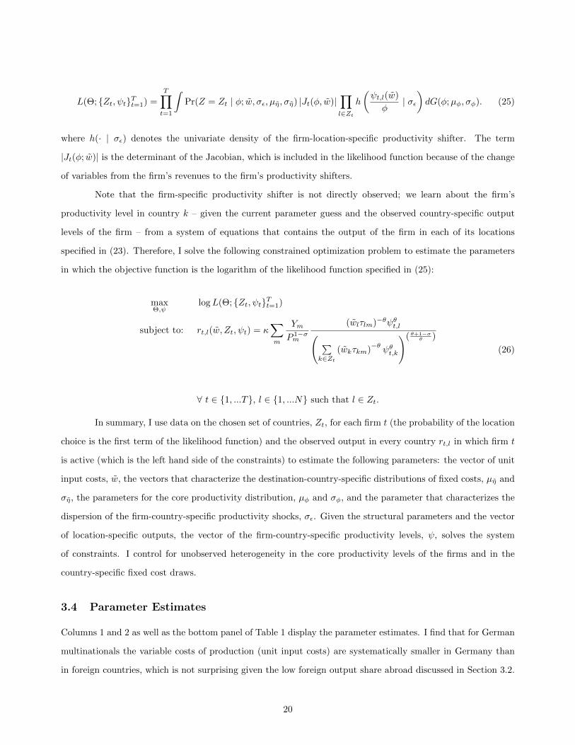
in which the objective function is the logarithm of the likelihood function specified in (25):

maxΘ,ψ

logL(Θ; Zt, ψtTt=1)

subject to: rt,l(w, Zt, ψt) = κ∑m

Ym

P 1−σm

(wlτlm)−θψθt,l( ∑k∈Zt

(wkτkm)−θψθt,k

)( θ+1−σθ )

∀ t ∈ 1, ...T, l ∈ 1, ...N such that l ∈ Zt.

(26)

In summary, I use data on the chosen set of countries, Zt, for each firm t (the probability of the location

choice is the first term of the likelihood function) and the observed output in every country rt,l in which firm t

is active (which is the left hand side of the constraints) to estimate the following parameters: the vector of unit

input costs, w, the vectors that characterize the destination-country-specific distributions of fixed costs, µη and

ση, the parameters for the core productivity distribution, µφ and σφ, and the parameter that characterizes the

dispersion of the firm-country-specific productivity shocks, σε. Given the structural parameters and the vector

of location-specific outputs, the vector of the firm-country-specific productivity levels, ψ, solves the system

of constraints. I control for unobserved heterogeneity in the core productivity levels of the firms and in the

country-specific fixed cost draws.

3.4 Parameter Estimates

Columns 1 and 2 as well as the bottom panel of Table 1 display the parameter estimates. I find that for German

multinationals the variable costs of production (unit input costs) are systematically smaller in Germany than

in foreign countries, which is not surprising given the low foreign output share abroad discussed in Section 3.2.

20

The unit input costs in Germany are normalized to one. The smallest difference in unit input costs is found in

Austria, in which German multinationals face only around five percent larger variable production costs than at

home. Within Western European countries, the production costs for German multinationals are largest in Italy

and the United Kingdom (23 percent higher than in Germany). The production costs in the United States are

around 35 percent higher than at home. The differences in production costs reflect both wage-level differences

and efficiency losses that occur by producing outside the home country. One would expect the efficiency losses

to be affected by the standard gravity variables (distance, contiguity, and language) and, accordingly, the unit

input costs show a tendency to rise with distance, and fall with contiguity and common language.

Table 1: Maximum Likelihood Estimates, Implied Fixed Costs, and Descriptive Statistics

Estimated Data

Country Unit input costs Fixed costs Mean fixed costs of Number Mean Medianw µη established affiliates of firms output output

Austria 1.051 3.544 6.796 91 76.3 34(0.022) (0.235) (0.779)

Belgium 1.150 3.859 9.904 45 235.3 37(0.054) (0.278) (2.768)

Canada 1.261 3.776 8.755 36 536.0 28.5(0.043) (0.222) (1.761)

Switzerland 1.155 3.462 6.050 70 58.3 17(0.023) (0.243) (1.156)

Spain 1.155 3.207 7.632 117 191.9 32(0.019) (0.229) (1.198)

France 1.152 3.227 7.287 191 107.7 30(0.015) (0.179) (0.729)

United Kingdom 1.234 3.176 7.204 121 119.4 23(0.016) (0.234) (1.096)

Ireland 1.106 4.054 5.438 18 36.3 19.5(0.045) (0.323) (1.299)

Italy 1.235 3.284 7.072 100 65.0 27.5(0.023) (0.221) (0.972)

Netherlands 1.118 3.724 7.927 46 83.1 25(0.024) (0.246) (1.650)

United States 1.353 3.205 6.798 211 569.0 26(0.023) (0.175) (0.825)

S.d. log fixed cost, ση 1.086 Scale parameter productivity, µφ 0.783(0.107) (0.003)

Shape parameter productivity, σφ 6.436 S.d. log productivity shock, σε 0.108(0.313) (0.005)

Log-Likelihood -9.86E+03 Number of firms, T 9288

Notes: Unit costs in Germany are normalized to one. Standard errors in parentheses. Figures in columns 3, 5, and 6 are inmillion Euro. The 665 German MNEs mean (median) output in Germany is 625.8 million Euro (98 million Euro). Source:MiDi database and own calculations.

We can give the fixed costs a value interpretation as we observe the firms’ output in Euro and, with

CES preferences and monopolistic competition, we can easily determine that variable profits are proportional

21

to output. Fixed costs are identified by observing the actual choice of production locations and variable profits

together with the counterfactual scenarios of how variable profits would change if the firm altered its set of

production locations. Note that my model does not distinguish between fixed costs to maintain a plant and

sunk costs to establish a foreign plant. I use the parameter estimates together with the structure of the model

to calculate the mean fixed costs paid by firms that set up a production location in the respective countries.

The calculation of the mean fixed cost conditional on having established a plant in the country is described in

Appendix F, and the results are displayed in column 3 of Table 1. For most countries the estimated mean fixed

cost of plants that were actually established is 6-8 million Euro. The paid fixed cost is estimated to be larger

in Canada (8.8 million) and Belgium (9.9 million). The larger fixed cost estimates for these countries are in

accordance with the data displayed in columns 4 and 5 of Table 1. Belgium has almost the same geographic

location as the Netherlands and a similar local and surrounding market potential. While the number of German

firms that have production locations in these countries is about the same, the output of affiliates in Belgium

is much larger. These differences result in lower estimated variable production costs in Belgium, but larger

fixed costs. The lower variable costs ensure larger firms in Belgium, while the larger fixed costs ensure that the

number of predicted entrants are comparable across countries. Similarly, only a small number of firms has a

plant in Canada, but they tend to have very large outputs. Unlike the unit input costs, the fixed cost estimates

do not show a tendency to rise with distance from the host countries.

As discussed in the model section, the analysis in this paper abstracts away from fixed costs of market

access. To conduct a sensitivity analysis on how the lack of fixed cost of market access may affect the estimation

results, I carry out the following experiment: Suppose the estimated parameters in Table 1 are the true param-

eters of the data generating process. However, in addition suppose there are also fixed costs of market access,

ιmwi = ι. I simulate data from this extended model with fixed costs of market access (see footnote 16 on how

to include fixed costs of market access), and then estimate the regular model without such fixed costs of market

access. If the estimated parameters are very close to the true parameters, the bias from a lack of fixed costs of

market access does not seem to be severe. An obvious question is how large the fixed costs of market access

should be. Bernard, Jensen, and Schott (2009) report that on average the export volume by US firms that

serve only a single market was about 250k USD in year 2000. Assuming that operating profits are 20 percent of

sales, it seems unlikely that the fixed costs of market access for those firms exceeded 50k USD (which was about

52.5k Euro in year 2000), otherwise they would incur losses from exporting. I estimate the sensitivity of my

parameter estimates to fixed costs of market access of 50k, 100k, 200k and 300k Euro. Table 10 in Appendix C

presents the results. For reasonable fixed costs of market access (50k - 100k Euro), the estimated parameters are

very close to the true parameters. However for very large fixed cost of market access, the estimated parameters

overstate the the cost of the foreign input bundle – making firms appear less efficient abroad than they actually

22

are. Overall, these results suggest that for empirically plausible values of fixed marketing costs, ignoring such

costs is not likely to severely affect the other parameter estimates. Furthermore, I illustrate in Table 10 that

German MNEs’ share of export platform sales would vary only marginally from 0.39 to 0.37 between models

with these fixed costs of market access.

I also evaluate the robustness of the parameter estimates for German multinational firms to alternative

values of the parameter θ. Table 11 in Appendix C presents the results. The estimates are largely unchanged

for θ = 6 and θ = 9.

3.5 Decomposing the sources of home bias in production

Multinational firms have been characterized as footloose and free to reorganize their global operations as the

global economic environment changes [Caves (1996)].27 However, the evidence presented in Section 3.2 suggests

that this view of footloose multinationals is inaccurate, and, rather, firms show ‘home bias in production.’ Fur-

ther, while the copious literature on the proximity-concentration trade-off has provided evidence for the presence

of fixed costs, little is known about their quantitative importance. The parameter estimates above demonstrate

both significant fixed costs to starting production in a foreign country and higher variable production costs

abroad. In order to learn more about the quantitative importance of each of those barriers, in this section, I

let firms re-optimize their location decisions as well as their decisions about which market to serve from which

location, under different fixed and variable costs. I hold general equilibrium variables such as income and price

indices fixed as I change the cost parameters.

Table 2 contains the results. The model effectively fits the average share of foreign output across firms.

While in the data the average foreign output share is 0.29, in the estimated model the average foreign output

share is 0.28 percent. If the unit input costs in the foreign countries were the same as in Germany, and there

were no fixed costs for setting up foreign plants, then every firm would have a plant in each country, and the

average foreign output share across firms would be 0.87. The question arises as to whether fixed costs or larger

variable production costs abroad are the more important barrier to foreign production. If unit input costs were

equalized across countries, and fixed costs were kept at their estimated level, then firms would re-optimize their

production locations and output decisions such that the foreign output share would be 0.57. If, instead, fixed

costs were eliminated (and unit input costs held at their estimated level), the average foreign output share would

rise even further to 0.71. Overall, I find that both fixed costs and differences in unit input costs significantly

contribute to home bias in production. While both factors have a large quantitative effect, fixed costs are

slightly more important.

27See also The Economist on March 25, 2004: “Footloose firms: Are global companies too mobile for workers’ good?”

23

Table 2: Average share of foreign production in theoutput of German multinationals

Data Model Same unit No fixed No fixedinput costs as costs costs and samein Germany unit input costs

as in Germany

0.288 0.278 0.566 0.708 0.874(0.010) (0.023) (0.010) (0.003)

Notes: Trade costs and price indices are held fixed. Standard errors inparentheses.

4 Calibration

In the second tier of my empirical inquiry, I focus on general equilibrium welfare analysis. In this section, I

calibrate the key parameters to the general equilibrium outcomes of the model using data for many countries.

Specifically, I calibrate trade costs, variable foreign production costs, and fixed costs of setting up foreign

affiliates, to data on bilateral trade flows, the values of output of firms from country i in country l, and the

estimates of the country-specific variable production costs of German multinationals from the previous section.

The estimates of fixed and variable production costs for German multinationals from the previous section enable

me to include both variable foreign production frictions and fixed costs in the analysis. On the aggregate level,

both fixed costs of establishing foreign locations and higher variable production costs abroad discourage foreign

production, so separating the two barriers would be infeasible with information only about aggregate flows. I

solve for the endogenous relative wages and price indices in every country.

4.1 Additional Data

The analysis incorporates the same twelve Western European and North American countries as the previous sec-

tion. Data on multinational production comes from Ramondo, Rodrıguez-Clare, and Tintelnot (2015).28 Gross

manufacturing production and bilateral trade data comes from OECD STAN, and figures on labor endowments

are drawn from the Penn World Tables. Data on trade and multinational production (MP) are averages across

the years 1996 to 2001, and the figures on population are for the year 2000.

28Unlike bilateral trade flow data, data on production activities of multinationals in foreign countries is documented only sporad-ically. Ramondo, Rodrıguez-Clare, and Tintelnot (2015) construct a data set using data from UNCTAD on non-financial affiliatesales by firms from country i producing in country l. Since many of the country-pairs’ observations are missing, they interpolatemissing values using a regression of affiliate sales on the stock of M&A between these countries (which is available for a wider setof country-pairs). For the selected set of countries used in this paper, only 17 out of 132 country-pairs’ MP values in Ramondo,Rodrıguez-Clare, and Tintelnot (2015) were obtained via interpolation.

24

4.2 Calibration procedure

The model delivers predictions for MP and trade shares, which I use as moments to calibrate the parameters.29

The share of expenditures by consumers from country m that is spent on goods produced in country l (‘trade

share’) is

ξlm =Xlm

Ym, (27)

and the share of output produced by firms from country i in country l (‘MP share’) is

κil =

∑mXilm∑

mXlm

. (28)

The share of purchases of domestically produced goods and the share of production carried out by local

firms are included in these moments above. As an additional set of moments, I include the relative unit input

costs of German firms in various countries that were estimated in Section 3. These are driven both by the

foreign efficiency losses, γ, and endogenous relative wages, w. Relative variable production costs for German

(G) firms in country l are wlγGlwG

. Let wG denote the vector of such relative production costs for German

firms and ˆwG denote their estimates based on the German micro data in the previous section. The calibration

procedure (formally described below in (29)) aims to bring these expressions – as well as the MP share and

trade shares in the model and data– close to each other while simultaneously solving for endogenous wages by

solving the equilibrium constraints. Note that I do not impose the restriction that multinational firms from

other countries have the same variable production costs as German firms in the foreign host countries. Rather,

as specificed below, the variable effiency losses of multinational firms producing abroad are imposed to follow

a gravity pattern. Since wlγGlwG

contains wages, I cannot do a simple regression of ˆwG on gravity variables (but

instead need to solve the full model for each parameter guess to figure out what wages are; (29) solves exactly

that problem). The fixed cost estimates from Section 3 are not explicitly used in this procedure (only indirectly,

as they enabled the estimation of the variable production costs while controlling for fixed foreign production

costs).

I estimate the parameters that characterize the trade costs between countries l and m, τlm; efficiency

losses of foreign production, γil; and the distribution of fixed costs to set up plants in foreign countries as a firm

from country i, F i(η). I make the following restrictions on the functional form for trade and foreign production

iceberg costs:

τlm = βτconst(distlm)βτdist(βτcontig)

contiglm(βτlang)languagelm for l 6= m

γil = βγconst(distil)βγdist(βγcontig)

contigil(βγlang)languageil for i 6= l.

29The construction of MP and bilateral trade shares from the data is described in detail in Appendix B.

25

Domestic production iceberg costs and trade costs are normalized to one, while fixed costs for the

domestic production location are set to zero. For all l 6= i, the fixed costs to set up a plant in location l for a

firm from i (in units of labor in the destination country) are drawn independently across firms and locations.

Formally, ηil ∼ logN (ln ηil, βηdisp), where

ηil = βηconst(distil)βηdist(βηcontig)

contigil(βηlang)languageil for i 6= l.

The mass of firms in country i, Mi, and the size of the labor force, Li, are set proportional to the

population in country i. As in the previous section, the value for the dispersion parameter of the product level

productivity shock distribution, θ, is set to seven, and the elasticity of substitution, σ, is fixed to six. The shape

parameter of the core productivity level distribution, σφ, and the dispersion parameter of firm-location specific

productivity shocks, σε, are set to the estimates obtained from the German micro-data in the previous section.

The three sets of moments are stacked into the following vector:

d(β,w,A) =

ξ(β,w,A)− ξ

κ(β,w,A)− κ

wG(β,w,A)− ˆwG.

This vector d(β) is a 300 × 1 vector in which each element characterizes the distance between the

respective model outcome (given the parameter vector β) and the outcome in the data. The calibration’s

objective is to minimize the sum of the squared differences between the model outcomes and the data targets

for these outcomes. As we vary the parameter vector β, the equilibrium values of wages, profits (income), and

price indices change. Note that in order for firms to choose their optimal policy, only the equilibrium wages and

the market demand Am = YmP 1−σm

need to be known. Let Am(β,A,w) denote the market demand in country m

that comes out of the policy functions of the firms and equations (20) and (18). Searching for an equilibrium,

we seek a vector of market demands A and wages w such that Am(β,A,w) = Am ∀m = 1, ..., N , and the

labor market clearing condition, Ldl (β,A,w) = Ll ∀l = 1, ..., N − 1, which is specified in (19), holds. As in the

previous section, this suggests a constrained optimization procedure to calibrate the parameters.

Formally, the calibration solves the following constrained optimization problem:

minβ,w,A

d(β,w,A)′d(β,w,A)

subject to:

Am(β,w,A) = Am ∀m = 1, ..., N

Ldl (β,w,A) = Ll ∀l = 1, ..., N − 1.

(29)

26

As only relative wages matter, I normalize one country’s wages and drop one labor market clearing

condition. As I have 300 moments as targets and only 9 parameters, an obvious question is how to weight these

moments. I decide to be agnostic and give each moment the same weight.

I also calibrate a special case of my model in which the fixed costs to set up foreign plants are set to

infinity. Here, I simply choose the parameters of the trade cost function that provide the best fit to the data

on aggregate trade shares. As no multinational production arises under this restriction, I call this the ‘pure

trade model.’ It is observationally equivalent to the model by Anderson and van Wincoop (2003) in terms of

aggregate trade flows between countries.30 Using only the trade shares as the targets, I calibrate the same

gravity parameters of the trade cost function for this restricted model. In addition, I calibrate two other special

cases of my model - a model without fixed costs of foreign production and a model without the possibility

of export platform sales. The exact calibration procedure for these models is described in Appendix L and

Appendix M, respectively.

4.3 Calibration results

The parameter estimates for the global production model and the pure trade model are displayed in Table 3.

The sum of the squared deviations from the MP and trade shares in the data and calibrated model are displayed

under ‘Norm MP fit’ and ‘Norm trade fit’ in Table 3. What stands out is that the estimates of the trade barriers

are very similar across the two models. In both models, trade costs are rising with distance with an elasticity

of around .13.31 Note that the global production model no longer implies a gravity equation. Nevertheless,

both models fit the aggregate trade data similarly well and the gravity equation still provides a very good

approximation for the trade patterns in the global production model. Using the trade flows and trade costs

implied by the global production model, the R2 from regressing log trade flows on log trade costs and source

and destination fixed effects is 0.99. Furthermore, while the trade elasticity in the pure trade model is equal

to 1− σ = −5, in the global production model the trade elasticity is distinct but close (-5.38). That the trade

flows predicted by the global production model can be well approximated by the gravity trade model is not

entirely surprising. The global production model implies gravity to hold at the firm-level, but with firm-specific

multilateral resistance terms (i.e. the denominator of the second term and the third term of equation (10)),

which depend on which set of countries a firm has a plant. These firm-specific multilateral resistance terms

together with the fact that firms differ in the set of countries in which they have a plant imply that gravity

30If fixed costs of exporting were included, the restricted model with no multinational production would be equivalent to Chaney(2008).

31The distance parameter in the trade cost function is comparable to the distance elasticity of trade flows in the standard gravitymodel only after the elasticity of substitution is taken into account. The standard gravity trade model’s distance coefficient is(1 − σ)βτdist. Given σ = 6 and βτdist ≈ .13, the implied level of the distance coefficient is −.65, which is less than one standarddeviation away from the median distance coefficient estimate in the literature [see Table 3.4 in Head and Mayer (2014)]. A standardgravity regression with importer and exporter fixed effects leads to a comparable distance coefficient of −.6.

27

does not hold exactly in the aggregate. However, it does in a knife-edge case, when θ → σ − 1. In that case,

as discussed in the model section, the plants of the firms obtain their revenues from distinct products, so the

multilateral resistance is the same across firms, independent of the set of countries in which the firms have a

plant.

Table 3: Calibrated Parameters

Pure Trade Global Production No Export No Fixedmodel model Platform model Costs model

Trade costconstant, βτconst 0.723 0.781 0.940 0.796distance, βτdist 0.139 0.121 0.083 0.115language, βτlang 0.922 0.926 0.898 0.923

contiguity, βτcontig 0.934 0.931 0.906 0.937

Variable MP costconstant, βγconst 1.211 0.958 1.974distance, βγdist 0.004 0.028 0.015language, βγlang 0.984 0.964 0.988

contiguity, βγcontig 0.944 0.936 0.867

Fixed MP costconstant, βηconst 2.608 2.059distance, βηdist 0.000 0.000language, βηlang 0.851 0.186

contiguity, βηcontig 1.429 1.455

dispersion, βηdisp 0.262 1.091

Norm trade fit 0.258 0.242 0.224 0.221Norm MP fit 0.172 0.250 0.318

Identification of the variable MP cost parameters comes from the moments on variable production costs

for German multinational firms in different countries. In Figure 5 in the appendix, I compare German firms’

variable production costs in various destination countries implied by the calibrated model with the estimates

from the firm-level data in the previous section; the numbers are closely matched. The iceberg loss in foreign

production, γil, is calibrated to around 1.2 and lower in the case of contiguity and common language between

the firm’s country of origin, i, and the country of production, l. The identification of the fixed cost parameters

comes from the moments on bilateral MP shares. I present scatter plots on the model’s fit of trade and MP

shares in Appendix H. By contrast, the calibrated iceberg loss in foreign production, γil, is much larger (around

1.97) for a model without fixed costs of foreign production (Column 4 in Table 3).

28

4.4 Fit of export platform shares

The calibration is targeted to fit bilateral trade and MP shares, as well as the relative variable production costs

of German multinationals in various countries. How does the calibrated model perform with respect to moments

it did not try to fit? I use data from the BEA on the export platform share of US multinational firms in all

countries included in my estimation, other than the US, to compare the model’s predictions to the actual data.

While the model with no export platform sales predicts no export platform sales by construction, I compare the

predictions between the global production model and the special case with no fixed costs in Table 4. I find that

the global production model captures the export platforms shares relatively well, though it underpredicts export

platform sales in large economies (i.e Germany or Spain). Furthermore, I find that the export platform shares

are on average 1.2 times as large in the benchmark global production model as in the restricted model without

fixed costs. Why does the model with fixed costs of foreign production fit the export platform sales better?

Fixed costs cause firms to concentrate their production in fewer locations, which generates export platform

sales. In Appendix D, I show for a symmetric world how additional production locations lead to lower shares

of export platform sales.

Table 4: Export platform shares - Data and Models

Data Global Production No Fixedmodel Costs model

Austria 0.54 0.49 0.46Belgium 0.63 0.76 0.74Canada 0.37 0.30 0.23Switzerland 0.69 0.70 0.68Germany 0.47 0.21 0.16Spain 0.41 0.13 0.10France 0.37 0.24 0.19United Kingdom 0.34 0.20 0.15Ireland 0.80 0.66 0.63Italy 0.33 0.12 0.09Netherlands 0.62 0.52 0.48

Interestingly, the relationship between export platform sales and the number of production locations

of the firm depends on the parameter θ. I show in Table 12 in Appendix E that the export platform shares

are on average 1.6 times as large in the benchmark global production model as in the restricted model without

fixed costs for θ = 9. For higher θ there is more cannibalization between plants by the same firm, since the

productivity draws are less dispersed. However, going in the other direction, if there is more dispersion in the

productivity draws and in the limit, θ → σ − 1, there is no longer any cannibalization between plants, and the

number of plants by the firm would be unimportant for the export platform sales.

29

5 General equilibrium counterfactuals

I proceed by conducting counterfactual analysis. In each counterfactual, the general equilibrium is resolved for

the new parameter values. I contrast the counterfactual predictions of the global production model with the no

export platform model and with the no fixed costs model to illustrate the types of questions in which allowing

for export platform sales or fixed costs of foreign production changes the counterfactual general equilibrium

outcomes. I begin with an analysis of an important current policy issue.

5.1 Potential effects from a Canada-EU trade and investment agreement

In 2013 the EU and Canada reached a political agreement on the key elements of a trade and investment agree-

ment: CETA.32 What will be the effects of such an agreement – if it is signed – on the signatories and the US?

My setup is particularly suitable for addressing this question. As multinational firms tend to concentrate pro-

duction in just a few locations and serve the rest of the world via export platform sales, investment liberalization

agreements may have particularly strong third-country effects. Third-country effects arise in pure trade models

due to the terms of trade effects. With multinational production – in addition to the terms of trade effects – an

additional effect arises: the firm can directly move its production locations and volume between countries, so

the effect on third countries may be stronger as firms respond to changes in the global bilateral investment cost

structure. For instance, a European firm may want to have only one plant in North America. As investment

barriers to Canada fall, this firm may move its plant from the United States to Canada. This outcome would

be missed by models that do not take into account export platforms, since without export platforms the firm’s

decision to establish a plant in one country is independent of its investment decision in other countries.

Suppose a deep investment agreement can be reached that lowers both variable and fixed MP costs

between the EU countries and Canada by 20 percent. Table 5 displays the difference in the MP-shares before

and after the liberalization. The global production model predicts the aggregate MP-share of EU countries

in Canada would increase by 11.5 percent. US firms would react to higher Canadian wages and reduce their

investment in Canada such that the share of US production in Canada would fall from 16 to 12 percent. Finally,

the total foreign production in Canada would increase by a factor of 1.24. Simultaneously, part of the EU

countries’ increased investment in Canada would crowd out their previous production in the US. EU countries’

production share in the US would fall from 4.57 to 4.33 percent. In relative terms, this is a decline of 5 percent.

Canadian firms would react to higher relative wages in Canada and increase their activities in the US, but only

32Comprehensive Economic and Trade Agreement (CETA). Currently proposed measures to remove investment barriers betweenthe EU and Canada include increased investment protection, harmonization of regulation, the removal of barriers to executive labormobility, and improvement in access to information for foreign investors. More information from the Canadian government canbe found here: http://www.canadainternational.gc.ca/eu-ue/policies-politiques/trade_agreements-accords_commerciaux.

aspx?lang=eng. More information from the EU commission can be found here: http://trade.ec.europa.eu/doclib/press/index.

cfm?id=974.

30

by a small share compared to the decrease in EU firms’ activities.

In contrast, results from the model with no export platform sales predict that a Canada-EU trade and

investment agreement would lead to no significant delocation effects of EU multinationals’ production in the US.

This is because without export platform sales, the only channel for an agreement to affect EU multinationals’

production is through changes in wage and price indices across countries, which only lead to minor changes in

EU production shares in the US. Similarly, the delocation effect of production in the no fixed costs model is

substantially lower than in the global production model.

Across all models the predicted welfare changes are qualitatively similar. Canada would experience the

largest welfare gains. The welfare gains in EU countries would be positive but moderate in size and larger for

smaller countries. The US and Switzerland would experience small welfare losses. The US economy is large

enough that the aggregate welfare effects of even a substantial diversion of EU investment from the US to

Canada would be small.

Table 5: Counterfactual Changes of Lower EU-Canada MP Costs– Difference in inward MP shares

Global Production No Export No Fixedmodel Platform model Costs model

Canada United States Canada United States Canada United StatesCanada -7.51 0.01 -2.00 0.01 -6.43 0.00EU countries 11.51 -0.24 3.64 0.01 7.68 -0.02Switzerland -0.11 0.00 -0.02 0.00 -0.02 0.00United States -3.89 0.23 -1.62 -0.02 -1.23 0.01

Notes: Counterfactual: Reduction in variable and fixed MP costs between EU and Canada by 20 percent. Dif-ferences in MP shares: 100× (κ′il − κil); column: destination l, row: source i.

As a comparison to the potential effects from a Canada-EU agreement, I also compute the potential

effects of a hypothetical EU-US agreement that would lower variable and fixed foreign production costs between

the signatories by the same proportion. As expected given the differences in these countries’ relative sizes,

the effects on the non-signatory partners from such an agreement would be even larger: the share of EU

multinationals’ production in Canada would fall by one percentage point, and the welfare in Canada would fall

by about a quarter of a percent. Table 16 in the appendix contains the predicted outcomes for such an EU-US

agreement.

I proceed with the analysis of a classic question in the trade literature, which has been studied by Eaton

and Kortum (2002) among others: how large are the benefits of foreign technology?

31

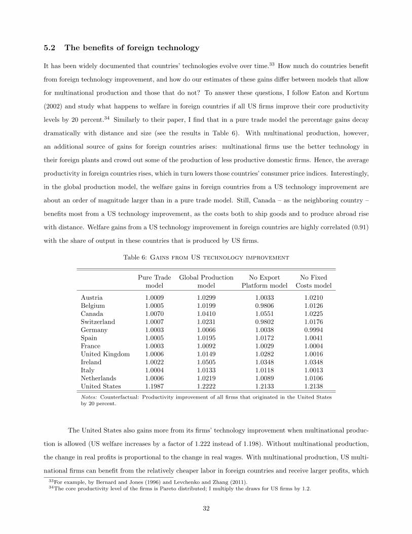
5.2 The benefits of foreign technology

It has been widely documented that countries’ technologies evolve over time.33 How much do countries benefit

from foreign technology improvement, and how do our estimates of these gains differ between models that allow

for multinational production and those that do not? To answer these questions, I follow Eaton and Kortum

(2002) and study what happens to welfare in foreign countries if all US firms improve their core productivity

levels by 20 percent.34 Similarly to their paper, I find that in a pure trade model the percentage gains decay

dramatically with distance and size (see the results in Table 6). With multinational production, however,

an additional source of gains for foreign countries arises: multinational firms use the better technology in

their foreign plants and crowd out some of the production of less productive domestic firms. Hence, the average

productivity in foreign countries rises, which in turn lowers those countries’ consumer price indices. Interestingly,

in the global production model, the welfare gains in foreign countries from a US technology improvement are

about an order of magnitude larger than in a pure trade model. Still, Canada – as the neighboring country –

benefits most from a US technology improvement, as the costs both to ship goods and to produce abroad rise

with distance. Welfare gains from a US technology improvement in foreign countries are highly correlated (0.91)

with the share of output in these countries that is produced by US firms.

Table 6: Gains from US technology improvement

Pure Trade Global Production No Export No Fixedmodel model Platform model Costs model

Austria 1.0009 1.0299 1.0033 1.0210Belgium 1.0005 1.0199 0.9806 1.0126Canada 1.0070 1.0410 1.0551 1.0225Switzerland 1.0007 1.0231 0.9802 1.0176Germany 1.0003 1.0066 1.0038 0.9994Spain 1.0005 1.0195 1.0172 1.0041France 1.0003 1.0092 1.0029 1.0004United Kingdom 1.0006 1.0149 1.0282 1.0016Ireland 1.0022 1.0505 1.0348 1.0348Italy 1.0004 1.0133 1.0118 1.0013Netherlands 1.0006 1.0219 1.0089 1.0106United States 1.1987 1.2222 1.2133 1.2138

Notes: Counterfactual: Productivity improvement of all firms that originated in the United Statesby 20 percent.

The United States also gains more from its firms’ technology improvement when multinational produc-

tion is allowed (US welfare increases by a factor of 1.222 instead of 1.198). Without multinational production,

the change in real profits is proportional to the change in real wages. With multinational production, US multi-

national firms can benefit from the relatively cheaper labor in foreign countries and receive larger profits, which

33For example, by Bernard and Jones (1996) and Levchenko and Zhang (2011).34The core productivity level of the firms is Pareto distributed; I multiply the draws for US firms by 1.2.

32

raises US consumer’s income. Note that the US welfare gains exceed 20 percent under a unilateral technology

improvement for US firms. In contrast, if all countries improve their firms’ technology by 20 percent, every

country’s welfare will simply rise by 20 percent (not displayed in the table). This implies, for different initial

conditions, e.g. after the increase in productivity of US firms, the welfare gains for the US from a technology

improvement in all countries other than the US could be negative, as US firms’ profits would decline.35

To summarize, in the global production model, since the level of technology used in a country’s pro-

duction is endogenous, an overall improvement in US firms’ technology improves the technology used in foreign

countries’ production. In other words, multinational firms enhance the spread of technology to foreign coun-

tries.36 The gains in foreign countries depend crucially on the cost of foreign production, which I carefully

estimate in this paper. The precise nature of the costs to foreign production is also important. The baseline

model systematically implies larger welfare gains abroad from the US technology improvement than does the

no fixed costs model. In models without multinational production, the cost of foreign production is infinite by

assumption, and the welfare gains abroad are estimated as even lower.

5.3 The gains from multinational production, trade, and openness

I continue by studying the gains from multinational production. I define as the gains from multinational

production the change in real income one finds when going from a version of the model with infinite costs of

multinational production to the model with the calibrated parameters. The relative changes in outcomes for

welfare, real wages, and real profits are displayed in Table 7. Interestingly, real wages and real profits respond

quite differently to the availability of multinational production. Real wages increase due to multinational

production, since multinational production substantially lowers the price index. In contrast, real profits fall

from allowing multinational production in almost all countries. Note that the effect of multinational production

on real profits is ambiguous. On the one hand, multinational production raises production efficiency and lowers

a multinational’s cost curve. On the other hand, the aggregate price index falls, which lowers demand, and

multinational firms bear the burden of fixed costs for multinational production. Furthermore, firms’ market

shares across countries are affected by multinational production. Firms from some countries are able to expand

their market shares due to multinational production at the expense of sales by firms from other countries. I

find that real profits in smaller countries tend to fall more than in larger countries because of the availability of

multinational production. Note that if fixed costs were zero, real profits would rise for firms in more countries

(see the results for the no fixed costs model in Table 7), since the share of profits in revenues would be higher.

35In Appendix N, I present levels of parameters for which my model can be solved analytically and show that whether the welfaregain of the country whose firms improved their technology exceeds the rate of technology improvement depends on the increase inglobal market share due to the technology improvement.

36The gains from foreign technology improvements may be even larger when spillovers are included. Poole (2013) finds evidencefor knowledge transfers from multinational to domestic firms in Brazilian matched worker-establishment data. Alfaro and Chen(2012) estimate that around 2/3 of the gains from multinational production arise through technology spillovers.

33

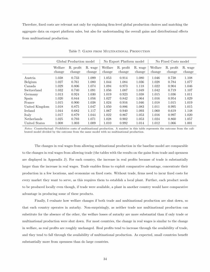
Therefore, fixed costs are relevant not only for explaining firm-level global production choices and matching the

aggregate data on export platform sales, but also for understanding the overall gains and distributional effects

from multinational production.

Table 7: Gains from Multinational Production

Global Production model No Export Platform model No Fixed Costs model

Welfare R. profit R. wage Welfare R. profit R. wage Welfare R. profit R. wagechange change change change change change change change change

Austria 1.038 0.733 1.099 1.053 0.914 1.080 1.046 0.738 1.108Belgium 1.027 0.761 1.080 1.044 1.084 1.036 1.028 0.784 1.077Canada 1.029 0.806 1.074 1.094 0.973 1.118 1.022 0.904 1.046Switzerland 1.032 0.740 1.091 1.056 1.087 1.049 1.042 0.719 1.107Germany 1.013 0.924 1.030 1.019 0.923 1.038 1.015 1.036 1.011Spain 1.020 0.844 1.056 1.027 0.842 1.064 1.016 0.954 1.029France 1.015 0.900 1.038 1.024 0.916 1.046 1.018 1.015 1.019United Kingdom 1.018 0.875 1.047 1.050 0.886 1.083 1.011 0.995 1.015Ireland 1.044 0.682 1.117 1.067 0.940 1.093 1.060 0.619 1.148Italy 1.017 0.879 1.044 1.022 0.867 1.053 1.016 0.997 1.020Netherlands 1.025 0.793 1.071 1.028 0.902 1.053 1.024 0.860 1.057United States 1.008 1.003 1.009 1.010 0.992 1.014 1.012 1.066 1.001

Notes: Counterfactual: Prohibitive costs of multinational production. A number in this table represents the outcome from the cali-brated model divided by the outcome from the same model with no multinational production.

The changes in real wages from allowing multinational production in the baseline model are comparable

to the changes in real wages from allowing trade (the tables with the results on the gains from trade and openness

are displayed in Appendix J). For each country, the increase in real profits because of trade is substantially

larger than the increase in real wages. Trade enables firms to exploit comparative advantage, concentrate their

production in a few locations, and economize on fixed costs. Without trade, firms need to incur fixed costs for

every market they want to serve, as this requires them to establish a local plant. Further, each product needs

to be produced locally even though, if trade were available, a plant in another country would have comparative

advantage in producing some of these products.

Finally, I evaluate how welfare changes if both trade and multinational production are shut down, so

that each country operates in autarky. Non-surprisingly, as neither trade nor multinational production can

substitute for the absence of the other, the welfare losses of autarky are more substantial than if only trade or

multinational production were shut down. For most countries, the change in real wages is similar to the change

in welfare, as real profits are roughly unchanged. Real profits tend to increase through the availability of trade,

and they tend to fall through the availability of multinational production. As expected, small countries benefit

substantially more from openness than do large countries.

34

6 Conclusion

My paper contributes to the literature on international trade and multinational firms by developing a new

framework that is less restrictive in its assumptions about where multinational firms can produce and sell, and

what cost structure they face. In particular, my model accounts for both export platform sales and the fixed

costs of establishing foreign plants. Existing quantitative models of trade and multinational production have

proven tractable only after excluding many of the strategies that firms actually use or shutting down mechanisms

that are almost universally thought to be important. My framework can be used for a wide range of possible

empirical applications with either firm-level or aggregate data.

The analysis with firm-level data documents that German multinational firms still produce a large share

of their global output in their home country, despite the fact that they are active in multiple countries. My

estimates on the variable efficiency losses to foreign production and increasing returns at the plant-level suggest

that a characterization of multinationals as footloose is inaccurate. Both differences in variable production

costs across countries and fixed costs of establishing foreign plants turn out to be important barriers to foreign

production for German multinational firms.

General equilibrium analysis reveals that multinational firms play an instrumental role in the transmis-

sion of technology improvements to foreign countries. As multinationals have the ability to re-optimize their

production locations and output decisions when the cost structure across countries changes, trade and invest-

ment agreements can have a significant third-country effect, which would be missed if multinational firms are

excluded from the analysis or modeled in a more restrictive way. My findings accord with the common percep-

tion that countries compete for multinational firms and that small countries would be hurt disproportionately if

a country nearby were to improve the conditions for multinationals from other countries, as this policy-change

induces a firm-delocation effect. My framework can be used to quantitatively investigate the implications of

such policies or other changes to the economic environment.

Overall, there are gains and losses from combining both fixed costs of foreign production and export

platform sales into one model. Export platform sales should not be ignored since they account for a large fraction

of output of firms’ foreign plants. I find that fixed costs of foreign production help to fit key moments of the

data and that the precise nature of the costs of foreign production is relevant for counterfactual predictions.

At the same time, some analytic tractability that is present in the models by Ramondo and Rodriguez-Clare

(2013) and Arkolakis, Ramondo, Rodriguez-Clare, and Yeaple (2013) is lost when including fixed costs of foreign

production. It is noteworthy that such tractability re-emerges for a special case of my model, if one is willing

to assume that θ → σ − 1. This increased tractability comes at a cost, however, since this special case also

looses some economic features, as there is no longer any cannibalization between plants within the firm under

this condition.

35

References

Alfaro, L., and M. X. Chen (2012): “Selection, Reallocation, and Spillover: Identifying the Sources of Gainsfrom Multinational Production,” Working Paper 18207, National Bureau of Economic Research.

Anderson, J. E., and E. van Wincoop (2003): “Gravity with Gravitas: A Solution to the Border Puzzle,”The American Economic Review, 93(1), pp. 170–192.

Antras, P., T. C. Fort, and F. Tintelnot (2014): “The Margins of Global Sourcing: Theory and Evidencefrom U.S. Firms,” Discussion paper, Harvard University.

Arkolakis, C., N. Ramondo, A. Rodriguez-Clare, and S. Yeaple (2013): “Innovation and Productionin the Global Economy,” NBER Working Papers 18972, National Bureau of Economic Research, Inc.

Baltagi, B. H., P. Egger, and M. Pfaffermayr (2008): “Estimating regional trade agreement effects onFDI in an interdependent world,” Journal of Econometrics, 145(1-2), 194–208.

Bernard, A. B., J. B. Jensen, and P. K. Schott (2009): “Importers, Exporters and Multinationals: APortrait of Firms in the U.S. that Trade Goods,” in Producer Dynamics: New Evidence from Micro Data,NBER Chapters, pp. 513–552. National Bureau of Economic Research, Inc.

Bernard, A. B., and C. I. Jones (1996): “Comparing Apples to Oranges: Productivity Convergence andMeasurement across Industries and Countries,” American Economic Review, 86(5), 1216–38.

Blonigen, B. A., R. B. Davies, G. R. Waddell, and H. T. Naughton (2007): “FDI in space: Spatialautoregressive relationships in foreign direct investment,” European Economic Review, 51(5), 1303–1325.

Buch, C. M., J. Kleinert, A. Lipponer, and F. Toubal (2005): “Determinants and effects of foreigndirect investment: evidence from German firm-level data,” Economic Policy, 20(41), 52–110.

Caves, R. (1996): Multinational Enterprise and Economic Analysis. Cambridge University Press, Cambridge,2nd edn.

Chaney, T. (2008): “Distorted Gravity: The Intensive and Extensive Margins of International Trade,” Amer-ican Economic Review, 98(4), 1707–21.

Cummings, J., J. Manyika, L. Mendonca, E. Greenberg, S. Aronowitz, R. Chopra, K. Elkin,S. Ramaswamy, J. Soni, and A. Watson (2010): Growth and competitiveness in the United States: Therole of its multinational companies. McKinsey Global Institute.

Dube, J.-P. H., J. T. Fox, and C.-L. Su (2012): “Improving the Numerical Performance of Static andDynamic Aggregate Discrete Choice Random Coefficients Demand Estimation,” Econometrica, 80(5), 2231–2267.

Eaton, J., and S. Kortum (2002): “Technology, Geography, and Trade,” Econometrica, 70(5), pp. 1741–1779.

Eaton, J., S. Kortum, and F. Kramarz (2011): “An Anatomy of International Trade: Evidence FromFrench Firms,” Econometrica, 79(5), 1453–1498.

Ekholm, K., R. Forslid, and J. R. Markusen (2007): “Export-Platform Foreign Direct Investment,”Journal of the European Economic Association, 5(4), 776–795.

Feinberg, S. E., and M. P. Keane (2006): “Accounting for the Growth of MNC-Based Trade Using aStructural Model of U.S. MNCs,” American Economic Review, 96(5), 1515–1558.

Fort, T. C. (2014): “Technology and Production Fragmentation: Domestic versus Foreign Sourcing,” Workingpaper.

Gale, D., and H. Nikaido (1965): “The Jacobian Matrix and Global Univalence of Mappings,” MathematischeAnnalen, 159, 81–93.

Grossman, G. M., E. Helpman, and A. Szeidl (2006): “Optimal integration strategies for the multinationalfirm,” Journal of International Economics, 70(1), 216–238.

36

Gumpert, A., A. Moxnes, N. Ramondo, and F. Tintelnot (2016): “Multinational Firms and ExportDynamics,” Discussion paper, University of Chicago, mimeo.

Hanson, G. H. (2005): “Market potential, increasing returns and geographic concentration,” Journal of In-ternational Economics, 67(1), 1–24.

Head, K., and T. Mayer (2004): “Market Potential and the Location of Japanese Investment in the EuropeanUnion,” The Review of Economics and Statistics, 86(4), 959–972.

(2015): “Brands in Motion: Estimating multinational frictions in the car industry,” mimeo.

Heiss, F., and V. Winschel (2008): “Likelihood approximation by numerical integration on sparse grids,”Journal of Econometrics, 144, 62–80.

Helpman, E., M. J. Melitz, and S. R. Yeaple (2004): “Export Versus FDI with Heterogeneous Firms,”American Economic Review, 94(1), 300–316.

Holmes, T. J. (2011): “The Diffusion of Wal-Mart and Economies of Density,” Econometrica, 79(1), 253–302.

Horstmann, I. J., and J. R. Markusen (1992): “Endogenous market structures in international trade(natura facit saltum),” Journal of International Economics, 32(1-2), 109–129.

Irarrazabal, A., A. Moxnes, and L. D. Opromolla (2009): “The Margins of Multinational Productionand the Role of Intra-firm trade,” CEPR Discussion Papers 7145, C.E.P.R. Discussion Papers.

Klose, A., and A. Drexl (2005): “Facility location models for distribution system design,” European Journalof Operational Research, 162(1), 4 – 29.

Kotz, S., and S. Nadarajah (2000): Extreme Value Distributions: Theory and Applications. Imperial CollegePress.

Levchenko, A. A., and J. Zhang (2011): “The Evolution of Comparative Advantage: Measurement andWelfare Implications,” NBER Working Papers 16806, National Bureau of Economic Research, Inc.

Melitz, M. J. (2003): “The Impact of Trade on Intra-Industry Reallocations and Aggregate Industry Produc-tivity,” Econometrica, 71(6), 1695–1725.

Morales, E., G. Sheu, and A. Zahler (2015): “Extended Gravity,” Princeton University Mimeo.

Muendler, M.-A., and S. O. Becker (2010): “Margins of Multinational Labor Substitution,” AmericanEconomic Review, 100(5), 1999–2030.

Neary, J. P. (2002): “Foreign Direct Investment and the Single Market,” Manchester School, 70(3), 291–314.

Poole, J. (2013): “Knowledge Transfers from Multinational to Domestic Firms: Evidence from Worker Mo-bility,” The Review of Economics and Statistics, 95(2), 393–406.

Ramondo, N., and A. Rodriguez-Clare (2013): “Trade, Multinational Production, and the Gains fromOpenness,” Journal of Political Economy, 121(2), 273 – 322.

Ramondo, N., A. Rodrıguez-Clare, and F. Tintelnot (2015): “Multinational Production: Data andStylized Facts,” American Economic Review, 105(5), 530–36.

Redding, S., and A. J. Venables (2004): “Economic geography and international inequality,” Journal ofInternational Economics, 62(1), 53–82.

Revelt, D., and K. Train (2000): “Customer-Specific Taste Parameters and Mixed Logit: Households’Choice of Electricity Supplier,” Economics Working Papers E00-274, University of California at Berkeley.

Rodrigue, J. (2014): “Multinational Production, Exports and Aggregate Productivity,” Review of EconomicDynamics, 17(2), 243–261.

37

Su, C.-L., and K. L. Judd (2012): “Constrained Optimization Approaches to Estimation of Structural Mod-els,” Econometrica, 80(5), 2213–2230.

Train, K. (2009): Discrete Choice Methods with Simulation. Cambridge University Press, 2nd edn.

Yeaple, S. R. (2003): “The complex integration strategies of multinationals and cross country dependenciesin the structure of foreign direct investment,” Journal of International Economics, 60(2), 293–314.

38

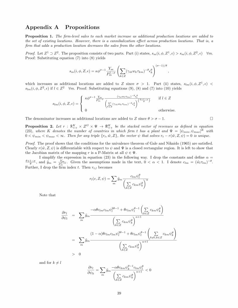
Appendix A Propositions

Proposition 1. The firm-level sales to each market increase as additional production locations are added tothe set of existing locations. However, there is a cannibalization effect across production locations. That is, afirm that adds a production location decreases the sales from the other locations.

Proof. Let Z1 ⊃ Z2. The proposition consists of two parts. Part (i) states, sm(i, φ, Z1, ε) > sm(i, φ, Z2, ε) ∀m.Proof: Substituting equation (7) into (8) yields

sm(i, φ, Z, ε) = κφσ−1 Ym

P 1−σm

(∑k∈Z

(γikwkτkm)−θεθk

)(σ−1)/θ

,

which increases as additional locations are added to Z since σ > 1. Part (ii) states, slm(i, φ, Z1, ε) <slm(i, φ, Z2, ε) if l ∈ Z2 ∀m. Proof: Substituting equations (9), (8) and (7) into (10) yields

slm(i, φ, Z, ε) =

κφσ−1 Ym

P 1−σm

(γilwlτlm)−θεθl( ∑k∈Z

(γikwkτkm)−θεθk

)( θ+1−σθ )

if l ∈ Z

0 otherwise.

The denominator increases as additional locations are added to Z since θ > σ − 1.

Proposition 2. Let r : RK++ × ZG × Ψ → RK++ be the stacked vector of revenues as defined in equation

(23), where K denotes the number of countries in which firm t has a plant and Ψ = [ψmin, ψmax]K with0 < ψmin < ψmax <∞. Then for any triple rt, w, Z, the vector ψ that solves rt − r(w, Z, ψ) = 0 is unique.

Proof. The proof shows that the conditions for the univalence theorem of Gale and Nikaido (1965) are satisfied.Clearly r(w, Z, ψ) is differentiable with respect to ψ and Ψ is a closed rectangular region. It is left to show thatthe Jacobian matrix of the mapping r is a P-Matrix at all ψ ∈ Ψ.

I simplify the expression in equation (23) in the following way. I drop the constants and define α =θ+1−σ

θ , and ym = YmP 1−σm

. Given the assumptions made in the text, 0 < α < 1. I denote clm = (wlτlm)−θ.

Further, I drop the firm index t. Then rt,l becomes

rl(c, Z, ψ) =∑m

ymclmψ

θl(∑

k∈Zckmψθk

)αNote that

∂rl∂ψl

=∑m

ym

−αθclmclmψ2θ−1l + θclmψ

θ−1l

(∑k∈Z

ckmψθk

)(∑k∈Z

ckmψθk

)α+1

=∑m

ym

(1− α)θclmclmψ2θ−1l + θclmψ

θ−1l

( ∑k 6=l,k∈Z

ckmψθk

)(∑k∈Z

ckmψθk

)α+1

> 0

and for k 6= l∂rl∂ψk

=∑m

ym−αθckmψθ−1

k clmψθl(∑

k∈Zckmψθk

)α+1 < 0

39

It is easy to see that at all ψ ∈ Ψ, | ∂rl∂ψl|ψl >

∑k 6=l| ∂rl∂ψk|ψk ∀l, hence the Jacobian matrix of r has a

dominant diagonal in the sense of Gale and Nikaido (1965). This along with the fact that ∂rl∂ψl

> 0 ∀l impliesthat the Jacobian matrix of r is a P-Matrix.

Then the univalence theorem of Gale and Nikaido (1965) implies whenever r(w, Z, a) = r(w, Z, b), wherea, b ∈ Ω, then a = b.

40

Appendix B Data

B.1 German multinationals data

All parent companies and majority-owned affiliates are from the manufacturing sector. Table 8 documents theaverage foreign production share by the number of production locations. Table 9 describes the average foreignproduction share and the average share of foreign production potential at the sector level.

Table 8: Foreign production shares by number ofproduction locations

Number of Number Mean share Mean shareproduction of firms of foreign of foreignlocations production production potential

2 474 0.26 0.37(0.20) (0.24)

3 102 0.32 0.54(0.18) (0.19)

4 40 0.35 0.65(0.19) (0.13)

5 23 0.39 0.71(0.16) (0.10)

6 14 0.46 0.75(0.15) (0.08)

≥7 12 0.48 0.80(0.06) (0.07)

all 665 0.29 0.44(0.20) (0.25)

Notes: Statistics for German MNE activities in 12 Western Europeanand North American countries. Standard deviations in parentheses.Source: MiDi database.

41

Table 9: Foreign production shares by sector

Sector Number Mean number Mean share Mean shareof firms of production of foreign of foreign

locations production production potential

Manufacture of ...

textiles 15 2.27 0.34 0.39(0.80) (0.22) (0.25)

Publishing, printing, and 22 2.36 0.26 0.37reproduction of recorded media (0.66) (0.25) (0.23)

chemicals and chemical products 85 3.05 0.33 0.45(1.79) (0.22) (0.26)

rubber and plastic products 67 2.73 0.32 0.45(1.21) (0.21) (0.25)

other non-metallic mineral products 23 2.65 0.39 0.34(1.19) (0.24) (0.21)

basic metals 31 2.35 0.22 0.40(0.66) (0.14) (0.24)

metal products 72 2.32 0.27 0.43(0.78) (0.17) (0.23)

machinery and equipment 138 2.49 0.25 0.46(1.16) (0.17) (0.26)

electrical machinery and apparatus 34 2.79 0.26 0.48(1.65) (0.17) (0.26)

radio, television, and communication 15 2.33 0.24 0.51equipment and apparatus (0.72) (0.16) (0.28)

medical, precision, and optical instruments, 49 2.33 0.30 0.54watches, and clocks (0.75) (0.20) (0.24)

motor vehicles, trailers and semi-trailers 57 2.82 0.30 0.48(1.28) (0.21) (0.25)

all 665 2.57 0.29 0.44(1.20) (0.20) (0.25)

Notes: Statistics for German MNE activities in 12 Western European and North American countries. Standard deviations inparentheses. Statistics are displayed for sectors with more than 10 German multinationals. Source: MiDi database.

B.2 Aggregate data

This appendix describes the construction of the trade and MP shares. All data comes from Ramondo, Rodrıguez-Clare, and Tintelnot (2015). The trade data is for the manufacturing sector only, while the MP data covers theentire non-financial sector of the economy. I implicitly assume that the MP in the service sector is proportionalto the MP in the trade sector. The same assumption is made by Arkolakis, Ramondo, Rodriguez-Clare, andYeaple (2013). All data are averages over the years 1996-2001.

B.2.1 Trade shares

Absorptionm = GrossProductionm + TotalWorldImportsm − TotalWorldlExportsm − TotOtherImportsmwhere TotOtherImportsm represents the total imports by country m from countries not included in

the analysis.

42

TradeSharelm =Xlm

Absorptionm

B.2.2 MP shares

Let Yil denote the value of output produced in country l by firms originating from country i. The constructionof the MP shares takes into account that the set of countries included in this study is only a subset of the entireglobal economy (though an important part of it, with good local coverage, e.g. Western Europe and NorthAmerica). Further, the total production of firms at home is not directly observed. I therefore take data ongross non-financial production in the respective country, and subtract the MP from 50 other source countriescontained in Ramondo, Rodrıguez-Clare, and Tintelnot (2015), which has the same sectoral coverage. Thisgives me an estimate of the value of local production, Yii.

MPSharejl =Yjl∑

i∈CYil,

where C denotes the set of countries included in the analysis.

43

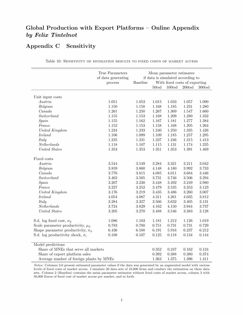
Global Production with Export Platforms – Online Appendixby Felix Tintelnot

Appendix C Sensitivity

Table 10: Sensitivity of estimation results to fixed costs of market access

True Parameters Mean parameter estimatesof data generating if data is simulated according to

process Baseline With fixed costs of exporting50tsd 100tsd 200tsd 300tsd

Unit input costsAustria 1.051 1.053 1.015 1.033 1.057 1.090Belgium 1.150 1.158 1.168 1.185 1.231 1.280Canada 1.261 1.250 1.267 1.369 1.547 1.660Switzerland 1.155 1.153 1.168 1.209 1.280 1.332Spain 1.155 1.162 1.167 1.181 1.277 1.384France 1.152 1.153 1.158 1.168 1.205 1.264United Kingdom 1.234 1.233 1.240 1.250 1.335 1.426Ireland 1.106 1.099 1.109 1.185 1.257 1.295Italy 1.235 1.231 1.237 1.246 1.315 1.413Netherlands 1.118 1.107 1.115 1.131 1.174 1.235United States 1.353 1.353 1.351 1.353 1.391 1.469

Fixed costsAustria 3.544 3.549 3.284 3.321 3.211 3.042Belgium 3.859 3.860 4.148 4.180 3.992 3.733Canada 3.776 3.815 4.085 4.011 3.684 3.446Switzerland 3.462 3.505 3.731 3.746 3.506 3.294Spain 3.207 3.230 3.448 3.492 3.249 2.980France 3.227 3.252 3.479 3.535 3.353 3.123United Kingdom 3.176 3.219 3.435 3.486 3.260 3.007Ireland 4.054 4.087 4.311 4.261 4.035 3.812Italy 3.284 3.327 3.566 3.632 3.405 3.131Netherlands 3.724 3.829 4.162 4.150 3.944 3.737United States 3.205 3.270 3.488 3.546 3.383 3.128

S.d. log fixed cost, ση 1.086 1.103 1.181 1.212 1.126 1.019Scale parameter productivity, µφ 0.783 0.780 0.751 0.731 0.731 0.729Shape parameter productivity, σφ 6.436 6.588 6.191 5.916 6.237 6.212S.d. log productivity shock, σε 0.108 0.107 0.125 0.118 0.134 0.144

Model predictionsShare of MNEs that serve all markets 0.352 0.247 0.162 0.124Share of export platform sales 0.392 0.388 0.380 0.374Average number of foreign plants by MNEs 1.363 1.375 1.396 1.411

Notes: Columns 2-6 present estimated parameter values if the data was generated by an augmented model with variouslevels of fixed costs of market access. I simulate 20 data sets of 10,000 firms and conduct the estimation on these datasets. Column 2 (Baseline) contains the mean parameter estimates without fixed costs of market access, column 3 with50,000 Euros of fixed cost of market access per market, and so forth.

1

Table 11: Estimation results: Robustness to different valuesof θ

Baseline Alternative values of θθ = 7 θ = 6 θ = 9

Unit input costsAustria 1.051 1.048 1.019Belgium 1.150 1.202 1.118Canada 1.261 1.246 1.296Switzerland 1.155 1.187 1.115Spain 1.155 1.162 1.145France 1.152 1.169 1.133United Kingdom 1.234 1.254 1.220Ireland 1.106 1.106 1.068Italy 1.235 1.242 1.239Netherlands 1.118 1.161 1.070United States 1.353 1.356 1.367

Fixed costsAustria 3.544 3.498 3.361Belgium 3.859 3.995 3.722Canada 3.776 3.843 3.696Switzerland 3.462 3.531 3.348Spain 3.207 3.212 3.066France 3.227 3.250 3.087United Kingdom 3.176 3.180 3.094Ireland 4.054 4.104 3.932Italy 3.284 3.298 3.231Netherlands 3.724 3.712 3.582United States 3.205 3.220 3.157

S.d. log fixed cost, ση 1.086 1.086 1.032Scale parameter productivity, µφ 0.783 0.700 0.854Shape parameter productivity, σφ 6.436 6.522 6.113S.d. log productivity shock, σε 0.108 0.110 0.103

Notes: This table contains the point estimation results for these alternative modelsbased on the German micro data.

2

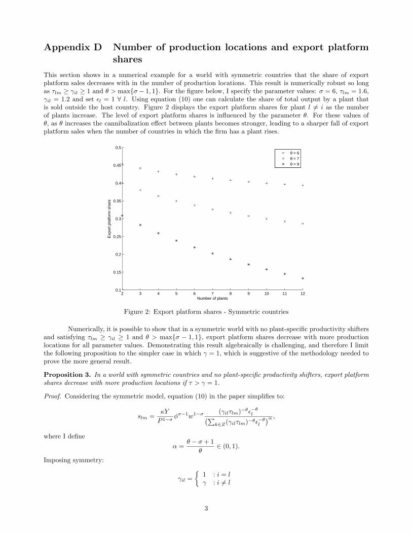
Appendix D Number of production locations and export platformshares

This section shows in a numerical example for a world with symmetric countries that the share of exportplatform sales decreases with in the number of production locations. This result is numerically robust so longas τlm ≥ γil ≥ 1 and θ > maxσ − 1, 1. For the figure below, I specify the parameter values: σ = 6, τlm = 1.6,γil = 1.2 and set εl = 1 ∀ l. Using equation (10) one can calculate the share of total output by a plant thatis sold outside the host country. Figure 2 displays the export platform shares for plant l 6= i as the numberof plants increase. The level of export platform shares is influenced by the parameter θ. For these values ofθ, as θ increases the cannibalization effect between plants becomes stronger, leading to a sharper fall of exportplatform sales when the number of countries in which the firm has a plant rises.

2 3 4 5 6 7 8 9 10 11 120.1

0.15

0.2

0.25

0.3

0.35

0.4

0.45

0.5

Number of plants

Exp

ort p

latfo

rm s

hare

θ = 6θ = 7θ = 9

Figure 2: Export platform shares - Symmetric countries

Numerically, it is possible to show that in a symmetric world with no plant-specific productivity shiftersand satisfying τlm ≥ γil ≥ 1 and θ > maxσ − 1, 1, export platform shares decrease with more productionlocations for all parameter values. Demonstrating this result algebraically is challenging, and therefore I limitthe following proposition to the simpler case in which γ = 1, which is suggestive of the methodology needed toprove the more general result.

Proposition 3. In a world with symmetric countries and no plant-specific productivity shifters, export platformshares decrease with more production locations if τ > γ = 1.

Proof. Considering the symmetric model, equation (10) in the paper simplifies to:

slm =κY

P 1−σ φσ−1w1−σ (γilτlm)−θε−θl(∑

k∈Z(γilτlm)−θε−θl)α ,

where I define

α =θ − σ + 1

θ∈ (0, 1).

Imposing symmetry:

γil =

1 : i = lγ : i 6= l

3

τlm =

1 : l = mτ : l 6= m

Eliminating plant-specific productivity shifters, one can write the following 4 cases of sales to local (sll),

sales to home (sli), sales to other countries with plants sothplantlm , and sales to other countries without plants

sothnoplantlm (suppressing other arguments for succinctness):

sll(K) =κY

P 1−σ φσ−1w1−σ γ−θ

((K − 1)(γτ)−θ + γ−θ + τ−θ)α

sli(K) =κY

P 1−σ φσ−1w1−σ (γτ)−θ

(K(γτ)−θ + 1)α

sothplantlm (K) =κY

P 1−σ φσ−1w1−σ (γτ)−θ

((K − 1)(γτ)−θ + γ−θ + τ−θ)α

sothnoplantlm (K) =κY

P 1−σ φσ−1w1−σ (γτ)−θ

(K(γτ)−θ + τ−θ)α,

where K denotes the number of foreign plants. Export platform shares are defined as:

ζ(K) = 1− sll(K)

sll(K) + sli(K) + (K − 1)sothplantlm (K) + (N −K − 1)sothnoplantlm (K)

= 1− γ−θ

γ−θ + (γτ)−θA(K) + (K − 1)(γτ)−θ + (N −K − 1)(γτ)−θB(K)

= 1− 1

1 + τ−θ (A(K) + (K − 1) + (N −K − 1)B(K)),

where

A(K) =((K − 1)(γτ)−θ + γ−θ + τ−θ)α

(K(γτ)−θ + 1)α

=

((K − 1)(γτ)−θ + γ−θ + τ−θ

K(γτ)−θ + 1

)αB(K) =

((K − 1)(γτ)−θ + γ−θ + τ−θ)α

(K(γτ)−θ + τ−θ)α

=

((K − 1)(γτ)−θ + γ−θ + τ−θ

K(γτ)−θ + τ−θ

)α.

Note that B(K) ≥ 1 ≥ A(K). Taking a derivative of ζ with respect to K:

ζ ′(K) =τ−θ (A′(K) + (1−B(K)) + (N −K − 1)B′(K))

(1 + τ−θ (A(K) + (K − 1) + (N −K − 1)B(K)))2

Imposing γ = 1:

A(K) =

(Kτ−θ + 1

Kτ−θ + 1

)α= 1

A′(K) = 0

B(K) =

(Kτ−θ + 1

(K + 1)τ−θ

)α> 1

B′(K) = α

(Kτ−θ + 1

(K + 1)τ−θ

)α−1(1− τθ

(K + 1)2

)< 0

B′(K) < 0 and N ≥ K + 1 implies that (N − K − 1)B′(K) ≤ 0. Therefore it is sufficient to show that

4

A′(K) + (1−B(K)) < 0 to demonstrate that ζ ′(K) < 0:

A′(K) + (1−B(K)) = 0 + 1− C(K)α

E(K)α

= 1−(Kτ−θ + 1

(K + 1)τ−θ

)α< 0

Where the last line follows because Kτ−θ + 1 > (K + 1)τ−θ whenever τ > 1. Therefore ζ ′(K) < 0.

In the general case without γ = 1 assumed, A′(K) > 0 and 1 − B(K) < 0. Therefore assessing therelative magnitudes of these terms would be crucial for determining the sign of A′(K) + (1−B(K)).

5

Appendix E Export platform sales statistics

Table 12: Export platform shares - Data and Models

Global Production No Fixed Costsmodel model

Country Data θ = 6 θ = 7 θ = 9 θ = 6 θ = 7 θ = 9

Austria 0.54 0.53 0.49 0.47 0.53 0.46 0.34Belgium 0.63 0.79 0.76 0.76 0.78 0.74 0.67Canada 0.37 0.35 0.30 0.23 0.31 0.23 0.14Switzerland 0.69 0.73 0.70 0.71 0.73 0.68 0.58Germany 0.47 0.23 0.21 0.19 0.21 0.16 0.10Spain 0.41 0.16 0.13 0.10 0.15 0.10 0.05France 0.37 0.27 0.24 0.21 0.25 0.19 0.12United Kingdom 0.34 0.23 0.20 0.17 0.20 0.15 0.09Ireland 0.80 0.70 0.66 0.65 0.69 0.63 0.54Italy 0.33 0.15 0.12 0.10 0.13 0.09 0.05Netherlands 0.62 0.56 0.52 0.51 0.54 0.48 0.38

Table 13: Export Platform shares:Model prediction for German

multinational firms

Country Export PlatformShare of Total Sales

Austria 0.42Belgium 0.64Canada 0.27Switzerland 0.50Spain 0.24Germany 0.11France 0.22United Kingdom 0.14Ireland 0.52Italy 0.09Netherlands 0.47United States 0.02

Notes: Export platform sales predictions forGerman MNEs based on estimates from theGerman micro data.

6

Appendix F Calculation of individual level parameters

The estimation in Section 3 delivers a distribution of fixed costs faced by the observed multinational firms.With these estimates I derive the distribution of fixed costs for each multinational firm conditional on itsobserved location choice, Zt, and the location-specific productivity vector, ψt. We can then calculate the meanvalue of fixed costs that were actually paid to set up a plant in the respective countries. To my knowledge,Revelt and Train (2000) were the first to use such a procedure to infer information about the tastes of eachsampled customer from the estimates of the distribution of tastes in the population with a nonlinear - mixedlogit - discrete choice model.

Let β denote the parameter vector of estimates in Section 3. The productivity vector across plants offirm t, ψt, can be calculated given rt and β. The density of the fixed cost draws across countries conditional onhaving chosen a plant in country l can be written as

u(f | Zt, ψt, β) =Pr(Zt | ψt, f)z(f | β)∫

fPr(Zt | ψt, f)z(f | β)df

,

where

Pr(Zt | ψt, f) =

∫φ

Pr(Zt | φ, f)k(φ | ψ)dφ,

and

k(φ | ψt) =g(φ)

∣∣∣dψt/φdψt

∣∣∣∏l∈Zt h(ψt,l(w,σε)

φ | β)∫φ′g(φ′)

∣∣∣dψt/φ′dψt

∣∣∣∏l∈Zt h(ψt,l(w,σε)

φ′ | β)dφ′,

and

Pr(Zt | φ, f) = 1Eε(Π|φ,Zt, ε, f ;β) ≥ Eε(Π|φ,Z ′, ε, f ;β) ∀Z ′.

The mean of fixed costs for firm t is

f t =

∫fu(f | Zt,l, ψt, β)df,

and the average fixed cost in country l of firms that actually have a plant there is

=

∑Tt=1 f

tl 1l ∈ Zt∑T

t=1 1l ∈ Zt.

7

Appendix G Computational Method

G.1 Optimization

The constrained optimization problems specified in (26) and (29) are solved using the numerical optimizationsolver Knitro.1 I hand-coded the analytical gradients (and checked their accuracy by comparison with a finitedifference approximation) and provided the sparsity structure of the problem. In order to find a global optimumto the problem, I started the optimization procedure from multiple starting points. Furthermore, I conducted aMonte Carlo study for the Maximum Likelihood Estimation in Section 3 to ensure that each of the parameterscan be recovered if the data process follows the specification of the model. Results for the Monte Carlo Studyare available from the author upon request.

G.2 Numerical Integration

The model contains three dimensions of firm heterogeneity: The core productivity level, φ, the vector of fixedunit labor requirements, η, and the vector of firm-country-specific productivity shifters, ε.

• Core productivity level

The core productivity level, φ, is distributed according to a Pareto distribution. I use a stratifiedrandom sampling method in order to obtain good coverage of relatively high productivity levels. I definethe following 10 intervals [0, .2, .4, .6, .8, .9, .95, .98, .99, .999, 1] and then draw S1/10 uniform randomnumbers within these intervals. The draws receive a weight inversely proportional to the length of theinterval. One can then obtain realizations from the Pareto distribution by using the draws of numbersbetween 0 and 1 and the inverse of the Pareto cdf.

• Firm-country-specific productivity shifter

The firm-country-specific productivity shifter, ε, is distributed according to a Log-Normal distribu-tion. The country-specific shocks affect smoothly the trade flows and revenues conditional on the locationchoice of the firm. They also affect smoothly the expected profit from a location choice. In orderto obtain good coverage of this N-dimensional shock while maintaining computational tractability, Iuse sparse grid points and Gaussian quadrature rules as basis functions. Sparse grid points break thecurse of dimensionality in high dimensional integration problems and for well behaved functions tendto be more accurate than Monte Carlo integration techniques. The approach is exact for polynomialfunctions of a given order. This approach is described by Heiss and Winschel (2008), and their web page(http://sparse-grids.de) provides the relevant code.

• Fixed cost draws

Similarly, the firm-country-specific fixed cost level, η, is distributed according to a Log-Normaldistribution. Since domestic fixed costs are zero, this is an N-1 dimensional vector. When simulating theintegrals in (15), (19), (20), and (21), I use a smoothed accept-reject simulator to maintain differentiabilityof the integrals while evaluating the integrals at a finite number of fixed cost draws. See section 5.6.2in Train (2009) for a more detailed description and discussion of advantages from this approach. Giventhe scale of the other variables, the goal is to set the smoothing parameter as low as possible subject tomaintaining numerical tractability. Following the notation in Train (2009), I use a smoothing parameterλ = 1 for the estimation with firm-level data in section 3 and a smoothing parameter λ = 0.01 for theestimation of the general equilibrium model in section 4 and the counterfactuals in section 5. The reasona different smoothing parameter is used is that the variables are in different scales in these sections.The current appraoch is equivalent to first rescaling all variables by 1/100 and then using a smoothingparameter of 0.01 in section 3. I use scrambled Halton sequences for the simulation of fixed cost draws,which again have better coverage than pseudo Monte Carlo draws.

1Su and Judd (2012) and Dube, Fox, and Su (2012) discuss advantages of this approach over a nested fixed point algorithm.

8

G.3 Estimation

The estimation is an implementation of the Mathematical Programming with Equilibrium Constraints (MPEC)procedure proposed by Su and Judd (2012). They show that the estimator is equivalent to a nested fixed-point estimator in which the inner loop solves for the firm-country-specific productivity levels, and the outerloop searches over parameters to maximize the likelihood. The estimator therefore inherits all the statisticalproperties of a nested fixed-point estimator. It is consistent and asymptotically normal as the number of firmstends to infinity and the number of simulation points used to evaluate the integrals rises proportionally to thenumber of firms.2 As there are 1,711 positive firm-country output observations of German multinationals, theconstrained optimization problem described in (26) has 1,711 equality constraints. For the purely domesticoperating German firms the inversion can be conducted analytically. In total, the data on the firm-outputobservations and the firms’ location set choices is used to estimate 26 structural parameters (15 parametersif the fixed cost distribution is assumed to be the same across host countries). I compute standard errors viabootstrapping and use a logit-smoothed accept-reject simulator to evaluate the probability of location choicedescribed in (21).3

G.4 Counterfactuals

To re-solve the system of equilibrium conditions for a new parameter vector, I again make use of the optimizationsolver Knitro but have the objective function take the value of a constant and the equilibrium conditionsrepresent the constraints.

2As the integrals are evaluated numerically in a finite sample with finite simulation draws, the Simulated Maximum LikelihoodEstimator is necessarily biased (after taking logarithms of the Likelihood function). I find in a Monte Carlo study of my estimationprocedure that the bias is very small in practice for this problem.

3See Train (2009), Chapter 5, for a description of this and other methods of simulation.

9

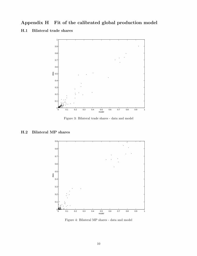
Appendix H Fit of the calibrated global production model

H.1 Bilateral trade shares

0 0.1 0.2 0.3 0.4 0.5 0.6 0.7 0.8 0.9 10

0.1

0.2

0.3

0.4

0.5

0.6

0.7

0.8

0.9

1

model

data

Figure 3: Bilateral trade shares - data and model

H.2 Bilateral MP shares

0 0.1 0.2 0.3 0.4 0.5 0.6 0.7 0.8 0.9 10

0.1

0.2

0.3

0.4

0.5

0.6

0.7

0.8

0.9

model

data

Figure 4: Bilateral MP shares - data and model

10

H.3 Variable production costs for German firms

1 1.05 1.1 1.15 1.2 1.25 1.3 1.35 1.41

1.05

1.1

1.15

1.2

1.25

1.3

1.35

1.4

Calibrated in model

Est

imat

es fr

om m

icro

dat

a

Figure 5: Variable production costs for German firms

H.4 Median fixed costs for German firms

0.75 0.8 0.85 0.9 0.95 1 1.05 1.1 1.15 1.2 1.253.1

3.2

3.3

3.4

3.5

3.6

3.7

3.8

3.9

4

4.1

calibrated in g.e. model

estim

ates

from

mic

ro d

ata

Figure 6: Median fixed costs for German firms

11

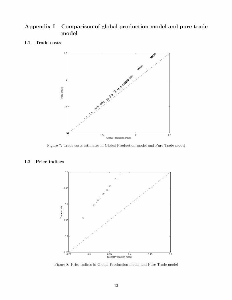
Appendix I Comparison of global production model and pure trademodel

I.1 Trade costs

1 1.5 2 2.51

1.5

2

2.5

Global Production model

Tra

de m

odel

Figure 7: Trade costs estimates in Global Production model and Pure Trade model

I.2 Price indices

0.25 0.3 0.35 0.4 0.45 0.50.25

0.3

0.35

0.4

0.45

0.5

Global Production model

Tra

de m

odel

Figure 8: Price indices in Global Production model and Pure Trade model

12

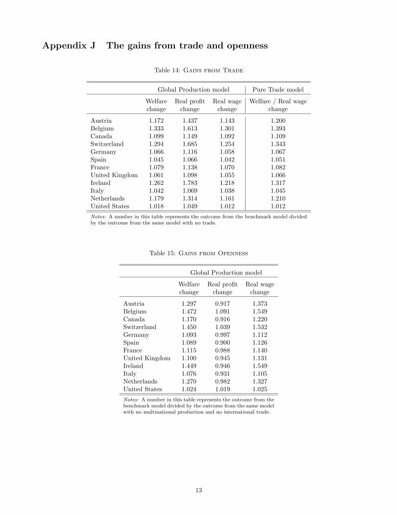
Appendix J The gains from trade and openness

Table 14: Gains from Trade

Global Production model Pure Trade model

Welfare Real profit Real wage Welfare / Real wagechange change change change

Austria 1.172 1.437 1.143 1.200Belgium 1.333 1.613 1.301 1.393Canada 1.099 1.149 1.092 1.109Switzerland 1.294 1.685 1.254 1.343Germany 1.066 1.116 1.058 1.067Spain 1.045 1.066 1.042 1.051France 1.079 1.138 1.070 1.082United Kingdom 1.061 1.098 1.055 1.066Ireland 1.262 1.783 1.218 1.317Italy 1.042 1.069 1.038 1.045Netherlands 1.179 1.314 1.161 1.210United States 1.018 1.049 1.012 1.012

Notes: A number in this table represents the outcome from the benchmark model dividedby the outcome from the same model with no trade.

Table 15: Gains from Openness

Global Production model

Welfare Real profit Real wagechange change change

Austria 1.297 0.917 1.373Belgium 1.472 1.091 1.549Canada 1.170 0.916 1.220Switzerland 1.450 1.039 1.532Germany 1.093 0.997 1.112Spain 1.089 0.900 1.126France 1.115 0.988 1.140United Kingdom 1.100 0.945 1.131Ireland 1.449 0.946 1.549Italy 1.076 0.931 1.105Netherlands 1.270 0.982 1.327United States 1.024 1.019 1.025

Notes: A number in this table represents the outcome from thebenchmark model divided by the outcome from the same modelwith no multinational production and no international trade.

13

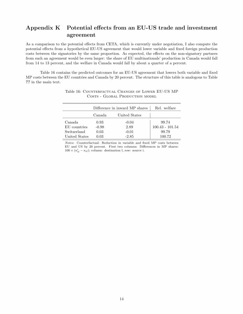
Appendix K Potential effects from an EU-US trade and investmentagreement

As a comparison to the potential effects from CETA, which is currently under negotiation, I also compute thepotential effects from a hypothetical EU-US agreement that would lower variable and fixed foreign productioncosts between the signatories by the same proportion. As expected, the effects on the non-signatory partnersfrom such an agreement would be even larger: the share of EU multinationals’ production in Canada would fallfrom 14 to 13 percent, and the welfare in Canada would fall by about a quarter of a percent.

Table 16 contains the predicted outcomes for an EU-US agreement that lowers both variable and fixedMP costs between the EU countries and Canada by 20 percent. The structure of this table is analogous to Table?? in the main text.

Table 16: Counterfactual Changes of Lower EU-US MPCosts - Global Production model

Difference in inward MP shares Rel. welfare

Canada United States

Canada 0.93 -0.04 99.74EU countries -0.98 2.89 100.43 - 101.54Switzerland 0.03 -0.01 99.79United States 0.03 -2.85 100.72

Notes: Counterfactual: Reduction in variable and fixed MP costs betweenEU and US by 20 percent. First two columns: Differences in MP shares:100× (κ′il − κil); column: destination l, row: source i.

14

Appendix L No Fixed Costs model

Here I present the results for a calibrated model without fixed costs of establishing foreign plants. Excludingfixed costs of foreign production implies that every firm establishes a plant in every country, which is obviouslycontrary to the firm-level evidence presented in Section 3. I calibrate the model to match aggregate tradeand MP shares (the variable production cost estimates for German multinationals are not included as targetsbecause those were estimated from a model with both fixed and variable costs).One can observe that this restricted model fits the MP data much worse compared to the full model in the maintext; it does a slightly better job at fitting the bilateral trade data, but the sum of the two norms of fit (sum ofsquared deviations of moments from model and data) is considerably higher.

Table 17: Calibrated Parameters

Model withoutFixed Costs of Production

Trade costconstant, βτconst 0.796distance, βτdist 0.115language, βτlang 0.923

contiguity, βτcontig 0.937

Variable MP costconstant, βγconst 1.974distance, βγdist 0.015language, βγlang 0.988

contiguity, βγcontig 0.867

Norm trade fit 0.221Norm MP fit 0.318

Table 18: Counterfactual Changes of Lower EU-CanadaMP Costs

Model without Fixed Costs of Production

Difference in inward MP shares Rel. welfare

Canada United States

Canada -6.43 0.00 101.44EU countries 7.68 -0.02 100.11 - 100.29Switzerland -0.02 0.00 99.97United States -1.23 0.01 99.98

Notes: Counterfactual: Reduction in variable MP costs between EU andCanada by 20 percent. First two columns: Differences in MP shares:100× (κ′il − κil); column: destination l, row: source i.

15

Table 19: Gains from US technology improvement

Relative to benchmark Relative to US gains

Model without Model withoutFixed Costs of Production Fixed Costs of Production

Austria 1.0210 9.80Belgium 1.0126 5.88Canada 1.0225 10.50Switzerland 1.0176 8.21Germany 0.9994 -0.27Spain 1.0041 1.93France 1.0004 0.17United Kingdom 1.0016 0.77Ireland 1.0348 16.29Italy 1.0013 0.59Netherlands 1.0106 4.96United States 1.2138 100.00

Notes: Counterfactual: Productivity improvement of all firms that originated in theUnited States by 20 percent. Columns 2: Welfare gains by country in percent relative towelfare gains in the United States.

Table 20: Gains from Multinational Production

Model withoutFixed Costs of Production

Welfare Real profit Real wagechange change change

Austria 1.046 0.738 1.108Belgium 1.028 0.784 1.077Canada 1.022 0.904 1.046Switzerland 1.042 0.719 1.107Germany 1.015 1.036 1.011Spain 1.016 0.954 1.029France 1.018 1.015 1.019United Kingdom 1.011 0.995 1.015Ireland 1.060 0.619 1.148Italy 1.016 0.997 1.020Netherlands 1.024 0.860 1.057United States 1.012 1.066 1.001

Notes: A number in this table represents the outcome from thebenchmark model divided by the outcome from the same modelwith no multinational production.

16

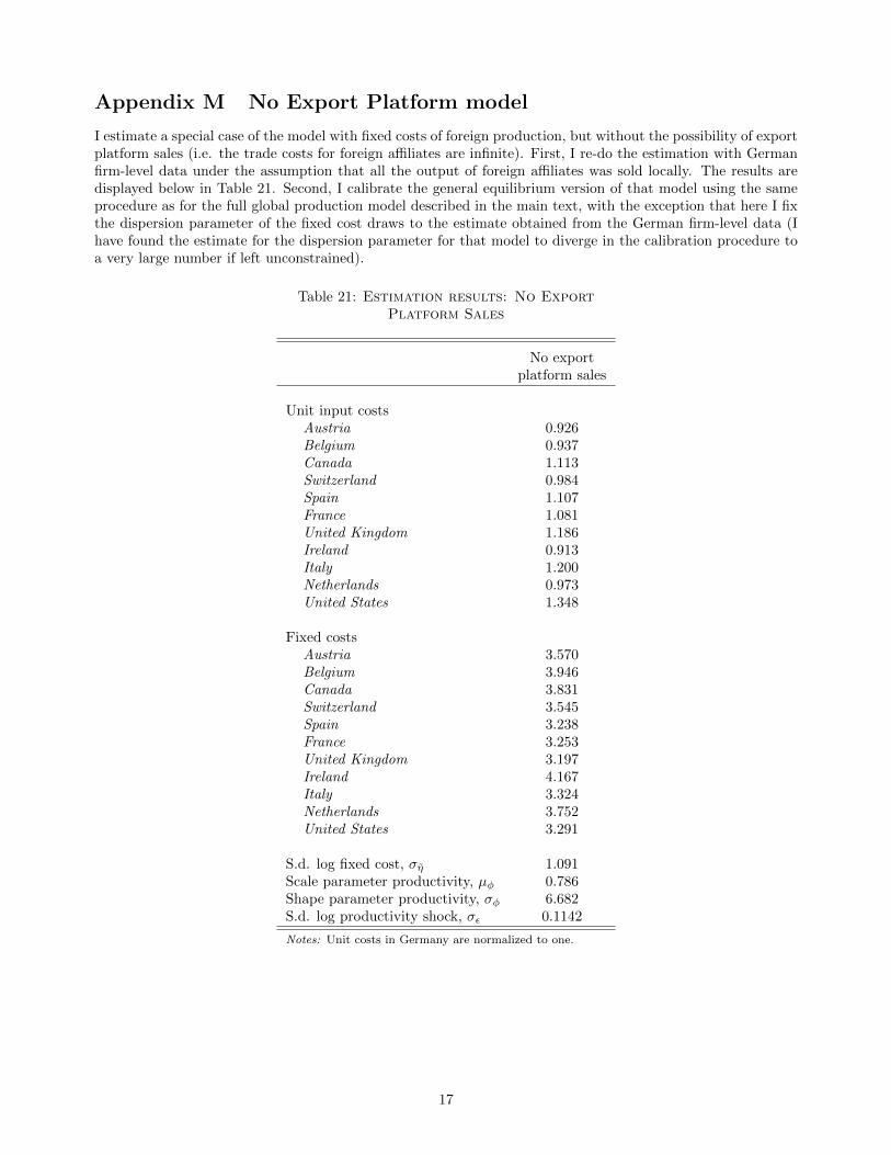
Appendix M No Export Platform model

I estimate a special case of the model with fixed costs of foreign production, but without the possibility of exportplatform sales (i.e. the trade costs for foreign affiliates are infinite). First, I re-do the estimation with Germanfirm-level data under the assumption that all the output of foreign affiliates was sold locally. The results aredisplayed below in Table 21. Second, I calibrate the general equilibrium version of that model using the sameprocedure as for the full global production model described in the main text, with the exception that here I fixthe dispersion parameter of the fixed cost draws to the estimate obtained from the German firm-level data (Ihave found the estimate for the dispersion parameter for that model to diverge in the calibration procedure toa very large number if left unconstrained).

Table 21: Estimation results: No ExportPlatform Sales

No exportplatform sales

Unit input costsAustria 0.926Belgium 0.937Canada 1.113Switzerland 0.984Spain 1.107France 1.081United Kingdom 1.186Ireland 0.913Italy 1.200Netherlands 0.973United States 1.348

Fixed costsAustria 3.570Belgium 3.946Canada 3.831Switzerland 3.545Spain 3.238France 3.253United Kingdom 3.197Ireland 4.167Italy 3.324Netherlands 3.752United States 3.291

S.d. log fixed cost, ση 1.091Scale parameter productivity, µφ 0.786Shape parameter productivity, σφ 6.682S.d. log productivity shock, σε 0.1142

Notes: Unit costs in Germany are normalized to one.

17

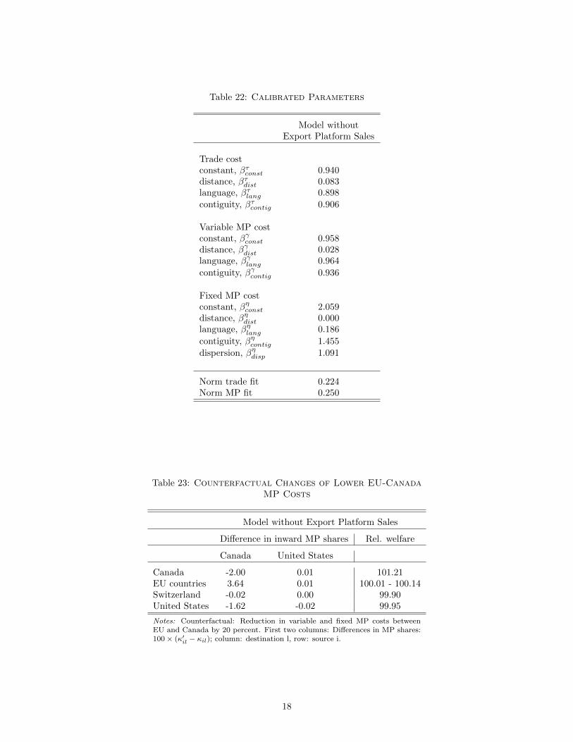
Table 22: Calibrated Parameters

Model withoutExport Platform Sales

Trade costconstant, βτconst 0.940distance, βτdist 0.083language, βτlang 0.898

contiguity, βτcontig 0.906

Variable MP costconstant, βγconst 0.958distance, βγdist 0.028language, βγlang 0.964

contiguity, βγcontig 0.936

Fixed MP costconstant, βηconst 2.059distance, βηdist 0.000language, βηlang 0.186

contiguity, βηcontig 1.455

dispersion, βηdisp 1.091

Norm trade fit 0.224Norm MP fit 0.250

Table 23: Counterfactual Changes of Lower EU-CanadaMP Costs

Model without Export Platform Sales

Difference in inward MP shares Rel. welfare

Canada United States

Canada -2.00 0.01 101.21EU countries 3.64 0.01 100.01 - 100.14Switzerland -0.02 0.00 99.90United States -1.62 -0.02 99.95

Notes: Counterfactual: Reduction in variable and fixed MP costs betweenEU and Canada by 20 percent. First two columns: Differences in MP shares:100× (κ′il − κil); column: destination l, row: source i.

18

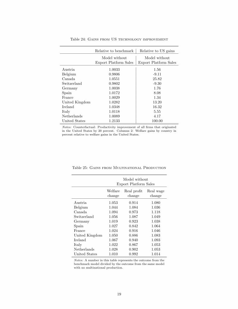
Table 24: Gains from US technology improvement

Relative to benchmark Relative to US gains

Model without Model withoutExport Platform Sales Export Platform Sales

Austria 1.0033 1.56Belgium 0.9806 -9.11Canada 1.0551 25.82Switzerland 0.9802 -9.30Germany 1.0038 1.76Spain 1.0172 8.08France 1.0029 1.34United Kingdom 1.0282 13.20Ireland 1.0348 16.32Italy 1.0118 5.55Netherlands 1.0089 4.17United States 1.2133 100.00

Notes: Counterfactual: Productivity improvement of all firms that originatedin the United States by 20 percent. Columns 2: Welfare gains by country inpercent relative to welfare gains in the United States.

Table 25: Gains from Multinational Production

Model withoutExport Platform Sales

Welfare Real profit Real wagechange change change

Austria 1.053 0.914 1.080Belgium 1.044 1.084 1.036Canada 1.094 0.973 1.118Switzerland 1.056 1.087 1.049Germany 1.019 0.923 1.038Spain 1.027 0.842 1.064France 1.024 0.916 1.046United Kingdom 1.050 0.886 1.083Ireland 1.067 0.940 1.093Italy 1.022 0.867 1.053Netherlands 1.028 0.902 1.053United States 1.010 0.992 1.014

Notes: A number in this table represents the outcome from thebenchmark model divided by the outcome from the same modelwith no multinational production.

19

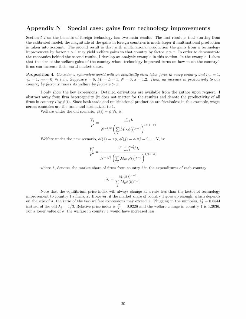
Appendix N Special case: gains from technology improvements

Section 5.2 on the benefits of foreign technology has two main results. The first result is that starting fromthe calibrated model, the magnitude of the gains in foreign countries is much larger if multinational productionis taken into account. The second result is that with multinational production the gains from a technologyimprovement by factor x > 1 may yield welfare gains to that country by factor y > x. In order to demonstratethe economics behind the second results, I develop an analytic example in this section. In the example, I showthat the size of the welfare gains of the country whose technology improved turns on how much the country’sfirms can increase their world market share.

Proposition 4. Consider a symmetric world with an identically sized labor force in every country and τlm = 1,γil = 1, ηil = 0, ∀i, l,m. Suppose σ = 6, Mi = L = 1, N = 3, x = 1.2. Then, an increase in productivity to onecountry by factor x raises its welfare by factor y > x.

I only show the key expressions. Detailed derivations are available from the author upon request. Iabstract away from firm heterogeneity (it does not matter for the results) and denote the productivity of allfirms in country i by φ(i). Since both trade and multinational production are frictionless in this example, wagesacross countries are the same and normalized to 1.

Welfare under the old scenario, φ(i) = φ ∀i, is:

Y1

P=

σσ−1L

N−1/θ

(∑i

Miκφ(i)σ−1

)1/(1−σ)

Welfare under the new scenario, φ′(1) = xφ, φ′(j) = φ ∀j = 2, ..., N , is:

Y ′1P ′

=

(σ−1+Nλ′1)σ−1 L

N−1/θ

(∑i

Miκφ′(i)σ−1

)1/(1−σ)

where λi denotes the market share of firms from country i in the expenditures of each country:

λi =Miφ(i)σ−1∑k

Mkφ(k)σ−1

Note that the equilibrium price index will always change at a rate less than the factor of technologyimprovement to country 1’s firms, x. However, if the market share of country 1 goes up enough, which dependson the size of σ, the ratio of the two welfare expressions may exceed x. Plugging in the numbers, λ′1 = 0.5544

instead of the old λ1 = 1/3. Relative price index is P ′

P = 0.9226 and the welfare change in country 1 is 1.2036.For a lower value of σ, the welfare in country 1 would have increased less.

20

Appendix O Global Production model – Sensitivity to alternativevalues for θ

Table 26: Calibrated Parameters –Sensitivity

Global Production model

θ = 6 θ = 7 θ = 9

Trade costconstant, βτconst 0.731 0.781 0.782distance, βτdist 0.133 0.121 0.118language, βτlang 0.916 0.926 0.927

contiguity, βτcontig 0.941 0.931 0.931

Variable MP costconstant, βγconst 1.249 1.211 1.076distance, βγdist 0.000 0.004 0.019language, βγlang 0.963 0.984 0.981

contiguity, βγcontig 0.964 0.944 0.955

Fixed MP costconstant, βηconst 3.361 2.608 3.037distance, βηdist 0.000 0.000 0.005language, βηlang 1.049 0.851 0.773

contiguity, βηcontig 1.206 1.429 1.362

dispersion, βηdisp 0.223 0.262 0.494

Norm trade fit 0.248 0.242 0.242Norm MP fit 0.182 0.172 0.165

Table 27: Counterfactual Changes of Lower EU-Canada MP Costs – Sensitivity

Global Production model

Difference in inward MP shares Rel. welfare

Canada United States

θ = 6 θ = 7 θ = 9 θ = 6 θ = 7 θ = 9 θ = 6 θ = 7 θ = 9

Canada -6.82 -7.51 -6.56 -0.00 0.01 0.02 101.65 101.82 101.58EU countries 9.78 11.51 10.94 -0.11 -0.24 -0.20 100.07 - 100.21 100.07 - 100.19 100.07 - 100.17Switzerland -0.07 -0.11 -0.09 0.00 0.00 0.00 99.95 99.93 99.92United States -2.89 -3.89 -4.28 0.11 0.23 0.18 99.96 99.96 99.96

Notes: Counterfactual: Reduction in variable and fixed MP costs between EU and Canada by 20 percent. Columns 1-6: Differences inMP shares: 100× (κ′il − κil); column: destination l, row: source i.

21

Table 28: Gains from US technology improvement – Sensitivity

Global Production model

Relative to benchmark Relative to US gains

θ = 6 θ = 7 θ = 9 θ = 6 θ = 7 θ = 9

Austria 1.0332 1.0299 1.0252 14.97 13.43 11.42Belgium 1.0244 1.0199 1.0124 11.00 8.96 5.62Canada 1.0362 1.0410 1.0446 16.32 18.47 20.26Switzerland 1.0291 1.0231 1.0139 13.11 10.40 6.30Germany 1.0074 1.0066 1.0048 3.35 2.95 2.17Spain 1.0187 1.0195 1.0170 8.43 8.78 7.70France 1.0103 1.0092 1.0066 4.65 4.13 3.00United Kingdom 1.0172 1.0149 1.0139 7.75 6.69 6.29Ireland 1.0643 1.0505 1.0412 28.94 22.73 18.70Italy 1.0135 1.0133 1.0112 6.10 5.98 5.08Netherlands 1.0238 1.0219 1.0180 10.72 9.84 8.19United States 1.2221 1.2222 1.2202 100.00 100.00 100.00

Notes: Counterfactual: Productivity improvement of all firms that originated in theUnited States by 20 percent. Columns 4-6: Welfare gains by country in percent rel-ative to welfare gains in the United States.

Table 29: Gains from Multinational Production – Sensitivity

Global Production model

Welfare change Real profit change Real wage change

θ = 6 θ = 7 θ = 9 θ = 6 θ = 7 θ = 9 θ = 6 θ = 7 θ = 9

Austria 1.036 1.038 1.035 0.700 0.733 0.773 1.104 1.099 1.087Belgium 1.028 1.027 1.026 0.725 0.761 0.788 1.088 1.080 1.074Canada 1.025 1.029 1.033 0.800 0.806 0.812 1.070 1.074 1.077Switzerland 1.034 1.032 1.030 0.698 0.740 0.774 1.101 1.091 1.081Germany 1.011 1.013 1.013 0.929 0.924 0.936 1.027 1.030 1.029Spain 1.016 1.020 1.022 0.850 0.844 0.850 1.050 1.056 1.056France 1.013 1.015 1.016 0.902 0.900 0.913 1.035 1.038 1.036United Kingdom 1.015 1.018 1.020 0.882 0.875 0.884 1.041 1.047 1.047Ireland 1.045 1.044 1.040 0.642 0.682 0.720 1.126 1.117 1.104Italy 1.013 1.017 1.017 0.888 0.879 0.886 1.038 1.044 1.044Netherlands 1.023 1.025 1.024 0.769 0.793 0.821 1.074 1.071 1.064United States 1.007 1.008 1.008 1.004 1.003 1.007 1.008 1.009 1.008

Notes: A number in this table represents the outcome from the benchmark model divided by the outcomefrom the same model with no multinational production.

22

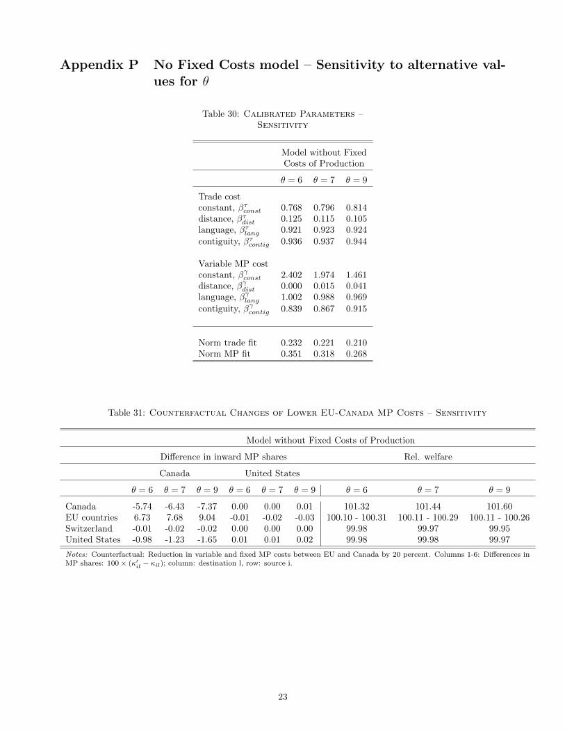
Appendix P No Fixed Costs model – Sensitivity to alternative val-ues for θ

Table 30: Calibrated Parameters –Sensitivity

Model without FixedCosts of Production

θ = 6 θ = 7 θ = 9

Trade costconstant, βτconst 0.768 0.796 0.814distance, βτdist 0.125 0.115 0.105language, βτlang 0.921 0.923 0.924

contiguity, βτcontig 0.936 0.937 0.944

Variable MP costconstant, βγconst 2.402 1.974 1.461distance, βγdist 0.000 0.015 0.041language, βγlang 1.002 0.988 0.969

contiguity, βγcontig 0.839 0.867 0.915

Norm trade fit 0.232 0.221 0.210Norm MP fit 0.351 0.318 0.268

Table 31: Counterfactual Changes of Lower EU-Canada MP Costs – Sensitivity

Model without Fixed Costs of Production

Difference in inward MP shares Rel. welfare

Canada United States

θ = 6 θ = 7 θ = 9 θ = 6 θ = 7 θ = 9 θ = 6 θ = 7 θ = 9

Canada -5.74 -6.43 -7.37 0.00 0.00 0.01 101.32 101.44 101.60EU countries 6.73 7.68 9.04 -0.01 -0.02 -0.03 100.10 - 100.31 100.11 - 100.29 100.11 - 100.26Switzerland -0.01 -0.02 -0.02 0.00 0.00 0.00 99.98 99.97 99.95United States -0.98 -1.23 -1.65 0.01 0.01 0.02 99.98 99.98 99.97

Notes: Counterfactual: Reduction in variable and fixed MP costs between EU and Canada by 20 percent. Columns 1-6: Differences inMP shares: 100× (κ′il − κil); column: destination l, row: source i.

23

Table 32: Gains from US technology improvement – Sensitivity

Model without Fixed Costs of Production

Relative to benchmark Relative to US gains

θ = 6 θ = 7 θ = 9 θ = 6 θ = 7 θ = 9

Austria 1.0199 1.0210 1.0215 9.39 9.80 9.91Belgium 1.0131 1.0126 1.0104 6.15 5.88 4.79Canada 1.0181 1.0225 1.0304 8.52 10.50 14.02Switzerland 1.0185 1.0176 1.0149 8.74 8.21 6.88Germany 0.9996 0.9994 0.9989 -0.18 -0.27 -0.52Spain 1.0029 1.0041 1.0061 1.39 1.93 2.83France 1.0004 1.0004 1.0000 0.20 0.17 0.02United Kingdom 1.0012 1.0016 1.0025 0.58 0.77 1.15Ireland 1.0340 1.0348 1.0352 16.04 16.29 16.25Italy 1.0008 1.0013 1.0019 0.39 0.59 0.89Netherlands 1.0095 1.0106 1.0113 4.48 4.96 5.24United States 1.2122 1.2138 1.2166 100.00 100.00 100.00

Notes: Counterfactual: Productivity improvement of all firms that originated in theUnited States by 20 percent. Columns 4-6: Welfare gains by country in percent rel-ative to welfare gains in the United States.

Table 33: Gains from Multinational Production – Sensitivity

Model without Fixed Costs of Production

Welfare change Real profit change Real wage change

θ = 6 θ = 7 θ = 9 θ = 6 θ = 7 θ = 9 θ = 6 θ = 7 θ = 9

Austria 1.047 1.046 1.041 0.731 0.738 0.751 1.111 1.108 1.100Belgium 1.031 1.028 1.025 0.776 0.784 0.804 1.082 1.077 1.069Canada 1.021 1.022 1.021 0.912 0.904 0.889 1.043 1.046 1.048Switzerland 1.047 1.042 1.034 0.702 0.719 0.751 1.116 1.107 1.090Germany 1.017 1.015 1.013 1.039 1.036 1.033 1.012 1.011 1.009Spain 1.017 1.016 1.014 0.968 0.954 0.929 1.027 1.029 1.031France 1.020 1.018 1.015 1.019 1.015 1.010 1.020 1.019 1.016United Kingdom 1.012 1.011 1.011 1.002 0.995 0.984 1.014 1.015 1.016Ireland 1.063 1.060 1.054 0.602 0.619 0.649 1.155 1.148 1.134Italy 1.017 1.016 1.013 1.007 0.997 0.979 1.019 1.020 1.020Netherlands 1.024 1.024 1.023 0.862 0.860 0.859 1.057 1.057 1.056United States 1.012 1.012 1.012 1.061 1.066 1.075 1.002 1.001 1.000

Notes: A number in this table represents the outcome from the benchmark model divided by the outcomefrom the same model with no multinational production.

24

Appendix Q No Export Platform model – Sensitivity to alternativevalues for θ

Table 34: Calibrated Parameters –Sensitivity

Model withoutExport Platform Sales

θ = 6 θ = 7 θ = 9

Trade costconstant, βτconst 0.936 0.940 0.954distance, βτdist 0.084 0.083 0.080language, βτlang 0.897 0.898 0.888

contiguity, βτcontig 0.909 0.906 0.907

Variable MP costconstant, βγconst 0.995 0.958 0.959distance, βγdist 0.023 0.028 0.028language, βγlang 0.966 0.964 0.983

contiguity, βγcontig 0.927 0.936 0.923

Fixed MP costconstant, βηconst 2.101 2.059 2.145distance, βηdist 0.050 0.000 0.000language, βηlang 0.172 0.186 0.124

contiguity, βηcontig 1.718 1.455 1.670

dispersion, βηdisp 0.924 1.091 1.072

Norm trade fit 0.222 0.224 0.225Norm MP fit 0.259 0.250 0.251

Table 35: Counterfactual Changes of Lower EU-Canada MP Costs – Sensitivity

Model without Export Platform Sales

Difference in inward MP shares Rel. welfare

Canada United States

θ = 6 θ = 7 θ = 9 θ = 6 θ = 7 θ = 9 θ = 6 θ = 7 θ = 9

Canada -1.92 -2.00 -2.15 0.01 0.01 0.01 101.24 101.21 101.25EU countries 3.58 3.64 3.81 0.01 0.01 0.01 100.01 - 100.15 100.01 - 100.14 100.01 - 100.15Switzerland -0.02 -0.02 -0.02 0.00 0.00 0.00 99.90 99.90 99.90United States -1.63 -1.62 -1.64 -0.01 -0.02 -0.02 99.95 99.95 99.95

Notes: Counterfactual: Reduction in variable and fixed MP costs between EU and Canada by 20 percent. Columns 1-6: Differences inMP shares: 100× (κ′il − κil); column: destination l, row: source i.

25

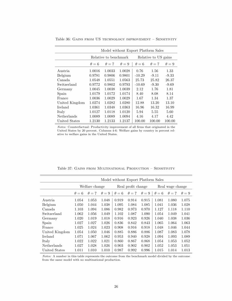
Table 36: Gains from US technology improvement – Sensitivity

Model without Export Platform Sales

Relative to benchmark Relative to US gains

θ = 6 θ = 7 θ = 9 θ = 6 θ = 7 θ = 9

Austria 1.0016 1.0033 1.0028 0.76 1.56 1.33Belgium 0.9781 0.9806 0.9801 -10.29 -9.11 -9.33Canada 1.0548 1.0551 1.0563 25.73 25.82 26.37Switzerland 0.9772 0.9802 0.9793 -10.69 -9.30 -9.69Germany 1.0045 1.0038 1.0039 2.12 1.76 1.81Spain 1.0179 1.0172 1.0174 8.40 8.08 8.14France 1.0036 1.0029 1.0029 1.67 1.34 1.37United Kingdom 1.0274 1.0282 1.0280 12.88 13.20 13.10Ireland 1.0361 1.0348 1.0363 16.96 16.32 16.99Italy 1.0127 1.0118 1.0120 5.94 5.55 5.60Netherlands 1.0089 1.0089 1.0094 4.16 4.17 4.42United States 1.2130 1.2133 1.2137 100.00 100.00 100.00

Notes: Counterfactual: Productivity improvement of all firms that originated in theUnited States by 20 percent. Columns 4-6: Welfare gains by country in percent rel-ative to welfare gains in the United States.

Table 37: Gains from Multinational Production – Sensitivity

Model without Export Platform Sales

Welfare change Real profit change Real wage change

θ = 6 θ = 7 θ = 9 θ = 6 θ = 7 θ = 9 θ = 6 θ = 7 θ = 9

Austria 1.054 1.053 1.048 0.919 0.914 0.915 1.081 1.080 1.075Belgium 1.050 1.044 1.038 1.095 1.084 1.085 1.041 1.036 1.028Canada 1.103 1.094 1.086 0.982 0.973 0.970 1.127 1.118 1.110Switzerland 1.062 1.056 1.049 1.102 1.087 1.090 1.054 1.049 1.041Germany 1.020 1.019 1.018 0.916 0.923 0.926 1.040 1.038 1.036Spain 1.027 1.027 1.026 0.836 0.842 0.843 1.065 1.064 1.063France 1.025 1.024 1.023 0.908 0.916 0.918 1.048 1.046 1.044United Kingdom 1.054 1.050 1.046 0.885 0.886 0.886 1.087 1.083 1.078Ireland 1.071 1.067 1.062 0.953 0.940 0.928 1.094 1.093 1.089Italy 1.022 1.022 1.021 0.860 0.867 0.868 1.054 1.053 1.052Netherlands 1.027 1.028 1.026 0.903 0.902 0.902 1.052 1.053 1.051United States 1.011 1.010 1.010 0.987 0.992 0.996 1.015 1.014 1.013

Notes: A number in this table represents the outcome from the benchmark model divided by the outcomefrom the same model with no multinational production.

26