NAVAL POSTGRADUATE SCHOOLThe United States Navy’s Military Sealift Command (MSC) employs its Combat Logistics Force (CLF) to supply the combatant fleet through replenishments at

NAVAL

POSTGRADUATE

SCHOOL

MONTEREY, CALIFORNIA

THESIS

Approved for public release; distribution is unlimited

ANALYZING UNDERWAY REPLENISHMENTS THROUGH SPATIAL MAPPING

by

Michael C. Blackman

December 2012

Thesis Advisor: Gerald G. Brown Second Reader: Walter C. DeGrange

THIS PAGE INTENTIONALLY LEFT BLANK

i

REPORT DOCUMENTATION PAGE Form Approved OMB No. 0704–0188 Public reporting burden for this collection of information is estimated to average 1 hour per response, including the time for reviewing instruction, searching existing data sources, gathering and maintaining the data needed, and completing and reviewing the collection of information. Send comments regarding this burden estimate or any other aspect of this collection of information, including suggestions for reducing this burden, to Washington headquarters Services, Directorate for Information Operations and Reports, 1215 Jefferson Davis Highway, Suite 1204, Arlington, VA 22202–4302, and to the Office of Management and Budget, Paperwork Reduction Project (0704–0188) Washington DC 20503. 1. AGENCY USE ONLY (Leave blank)

2. REPORT DATE December 2012

3. REPORT TYPE AND DATES COVERED Master’s Thesis

4. TITLE AND SUBTITLE ANALYZING UNDERWAY REPLENISHMENTS THROUGH SPATIAL MAPPING

5. FUNDING NUMBERS

6. AUTHOR(S) Michael C. Blackman 7. PERFORMING ORGANIZATION NAME(S) AND ADDRESS(ES)

Naval Postgraduate School Monterey, CA 93943–5000

8. PERFORMING ORGANIZATION REPORT NUMBER

9. SPONSORING /MONITORING AGENCY NAME(S) AND ADDRESS(ES) N/A

10. SPONSORING/MONITORING AGENCY REPORT NUMBER

11. SUPPLEMENTARY NOTES The views expressed in this thesis are those of the author and do not reflect the official policy or position of the Department of Defense or the U.S. Government. IRB Protocol number ______N/A______.

12a. DISTRIBUTION / AVAILABILITY STATEMENT Approved for public release; distribution is unlimited

12b. DISTRIBUTION CODE A

13. ABSTRACT (maximum 200 words) The United States Navy’s Military Sealift Command (MSC) employs its Combat Logistics Force (CLF) to supply the combatant fleet through replenishments at sea (RAS). These RAS events need to be conducted where the combatant fleet operates. In order to give logistics planners an accurate view of RAS locations, we create heat maps from historical RAS evolutions to illustrate and calculate the most probable location for future events. We compare relying on this estimated location with current practice of using the corresponding center point of a given Operational Area Box (OP Box) and determine the impact of this centroid location on CLF assets, fuel cost, and time. The Pacific Coast scenario that we present uses the Replenishment at-Sea Planner (RASP) to find the optimal scheduling of RAS events at both the OP Box center point and the estimated RAS location. The results show that the centroid location offers significant improvements in customer readiness and total CLF underway fuel usage planning.

14. SUBJECT TERMS Heat map, Replenishment at-Sea (RAS), Raster, Spatial Mapping, Centroid, Forecast, Combat Logistics Force (CLF)

15. NUMBER OF PAGES

61 16. PRICE CODE

17. SECURITY CLASSIFICATION OF REPORT

Unclassified

18. SECURITY CLASSIFICATION OF THIS PAGE

Unclassified

19. SECURITY CLASSIFICATION OF ABSTRACT

Unclassified

20. LIMITATION OF ABSTRACT

UU NSN 7540–01–280–5500 Standard Form 298 (Rev. 2–89) Prescribed by ANSI Std. 239–18

ii


iii

Approved for public release; distribution is unlimited

ANALYZING UNDERWAY REPLENISHMENTS THROUGH SPATIAL MAPPING

Michael C. Blackman Lieutenant, United States Navy

B.S., United States Naval Academy, 2005

Submitted in partial fulfillment of the requirements for the degree of

MASTER OF SCIENCE IN OPERATIONS RESEARCH

from the

NAVAL POSTGRADUATE SCHOOL December 2012

Author: Michael C. Blackman

Approved by: Gerald G. Brown Thesis Advisor

Walter C. DeGrange Second Reader

Robert F. Dell Chair, Department of Operations Research

iv


v

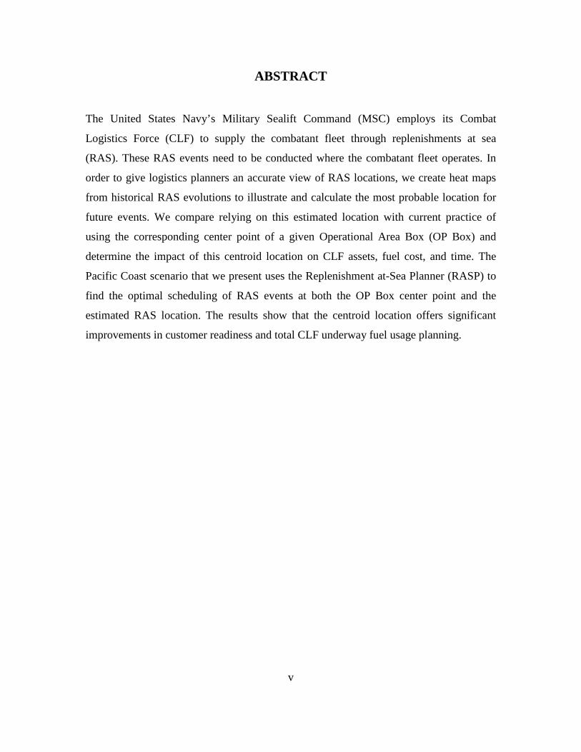
ABSTRACT

The United States Navy’s Military Sealift Command (MSC) employs its Combat

Logistics Force (CLF) to supply the combatant fleet through replenishments at sea

(RAS). These RAS events need to be conducted where the combatant fleet operates. In

order to give logistics planners an accurate view of RAS locations, we create heat maps

from historical RAS evolutions to illustrate and calculate the most probable location for

future events. We compare relying on this estimated location with current practice of

using the corresponding center point of a given Operational Area Box (OP Box) and

determine the impact of this centroid location on CLF assets, fuel cost, and time. The

Pacific Coast scenario that we present uses the Replenishment at-Sea Planner (RASP) to

find the optimal scheduling of RAS events at both the OP Box center point and the

estimated RAS location. The results show that the centroid location offers significant

improvements in customer readiness and total CLF underway fuel usage planning.

vi


vii

TABLE OF CONTENTS

I. INTRODUCTION........................................................................................................1 A. OVERVIEW OF COMBAT LOGISTICS FORCE ......................................1 B. HISTORICAL RESEARCH IN CLF REPLINISHMENT

PLANNING ......................................................................................................2 1. Initial Stages of CLF Planning ...........................................................2 2. Utilizing the CLF to Support Major Combat Operations and

Incorporating the CLF Planning Model ............................................2 3. Revolutionizing CLF Planning into an Operational Model .............4

C. DEFICIENCY OF DATA SUPPORTING RASP .........................................4 D. DEVELOPING A MORE ACCURATE MODEL TO FORECAST

REPLENISHMENT LOCATIONS ...............................................................6

II. HEAT MAP LITERATURE REVIEW .....................................................................7 A. THE ORIGIN OF THE HEAT MAP.............................................................7 B. HEAT MAPPING TYPES ..............................................................................7

1. Cluster Mapping ..................................................................................8 2. Raster Plotting ......................................................................................8

C. VALIDATING THE APPLICATION OF SPATIAL MAPPING ..............9 1. Exploring Road Incident Data with Heat Maps................................9 2. The Nested Process Model (NPM) ....................................................10

III. SPATIAL MAP AND CENTROID ALGORITHM ...............................................13 A. DISTRIBUTIONS OF HISTORICAL REPLENISHMENTS ..................13 B. BUSINESS RULES FOR DESIGNING RASTER PLOTS .......................14

1. Dimensions of an OP Box ..................................................................14 2. Creating Geographical Raster Plots .................................................15

a. Coordinate Referencing System .............................................15 b. Correlating Geographic Locations to Raster Cells ................15 c. Distortions From Map Projection ..........................................15

3. Cell Values and Weightings ..............................................................15 4. Forecasting a Future RAS Point in an OP Box ...............................16

C. ESTABLISHING SPATIAL MAPS FOR A PACIFIC COAST SCENARIO ....................................................................................................17 1. Defining OP Box Locations ...............................................................17 2. Data Sets .............................................................................................17

a. Partitioning the Data Sets .......................................................18 b. Training Set .............................................................................19 c. Test Set.....................................................................................19

3. OP Box Heat Maps.............................................................................19 a. MexiSocal ................................................................................20 b. CentCal ....................................................................................21 c. NorCal .....................................................................................22 d. PacNorWest .............................................................................23

viii

D. TESTING PACIFIC COAST SCENARIO WITH REPLENISHMENT AT SEA PLANNER (RASP) .....................................23 1. Routing Locations ..............................................................................24 2. Ships ....................................................................................................25

a. Ship Tracks ..............................................................................25 3. Scenario Overlay ................................................................................25

IV. ANALYSIS AND CONCLUSIONS .........................................................................27 A. CROSS-VALIDATION OF CENTROIDS .................................................27

1. Comparing Distances from Current Centroid Over Time ............27 2. Comparing Distances from Centroid and OP Box Center Point

to Successive RAS Locations .............................................................28 B. PACIFIC COAST SCENARIO RESULTS FROM RASP ........................29

1. Ships on Station in MXC and CCAL ...............................................30 2. Group of Ships Transiting from PNW to MXC ..............................31

C. CONCLUSION ..............................................................................................32 1. Summary .............................................................................................32 2. Recommendations for Future Research ..........................................32

a. Creating Scenario on Actual Historical Data ........................32 b. Include Exponential Weighting in Assigning Values of

RAS Events ..............................................................................32 c. Predicting Future RAS Locations through Time Series

Analysis....................................................................................33 d. Interfacing a Heat Map and Centroid Method into RASP ...33

APPENDIX A. SOLVER CUSTOMER PLANS COMPARISON OF ON-STATION RASP RUN ..............................................................................................35

APPENDIX B. SOLVER CUSTOMER PLANS COMPARISON OF STAGGERED TRANSIT RASP RUN.....................................................................37

LIST OF REFERENCES ......................................................................................................39

INITIAL DISTRIBUTION LIST .........................................................................................41

ix

LIST OF FIGURES

Figure 1. A CLF ship enters the OP Box from the top right corner, transits to center to conduct a RAS at the designated location, and then transits back out of OP Box to its previous entry location. ...............................................................5

Figure 2. A Business Tree Map. (Available from http://www.smartmoney.com, 2012). .................................................................................................................7

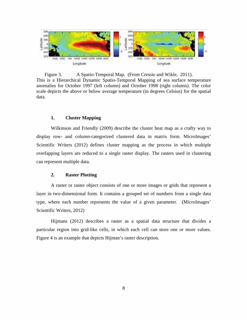
Figure 3. A Spatio-Temporal Map. (From Cressie and Wikle, 2011).............................8 Figure 4. A Raster Plot. (From National Center for Atmospheric Research (NCAR)

http://www.ncl.ucar.edu, 2012). ........................................................................9 Figure 5. The four-layer Nested Model. (From Munzner, 2009). ...................................10 Figure 6. Threats and validation in the nested model. (From Munzner, 2009). .............11 Figure 7. Possible distribution outcomes from sample RAS data within a random

11x11 dimensional area. RAS occurrences in each cell range from 0–40. Color shades increase from white (light) to red (dark). ...................................13

Figure 8. MexiSocal heat map. ........................................................................................20 Figure 9. CentCal heat map. ............................................................................................21 Figure 10. NorCal heat map. .............................................................................................22 Figure 11. PacNorWest heat map. .....................................................................................23 Figure 12. Routing locations for Pacific Coast Scenario in RASP. The last four

locations represent our calculated heat map centroid (HMC). ........................24 Figure 13. Pacific Coast Scenario Overlay. ......................................................................26 Figure 14. Distance from current centroid over successive RAS events. .........................28 Figure 15. Distances between current centroid and RAS events for each OP Box. ..........29

x


xi

LIST OF TABLES

Table 1. CLF ship classes and their speed in knots (KTS). (Data given from MSC website, http://www.msc.navy.mil/inventory, 2012). ......................................14

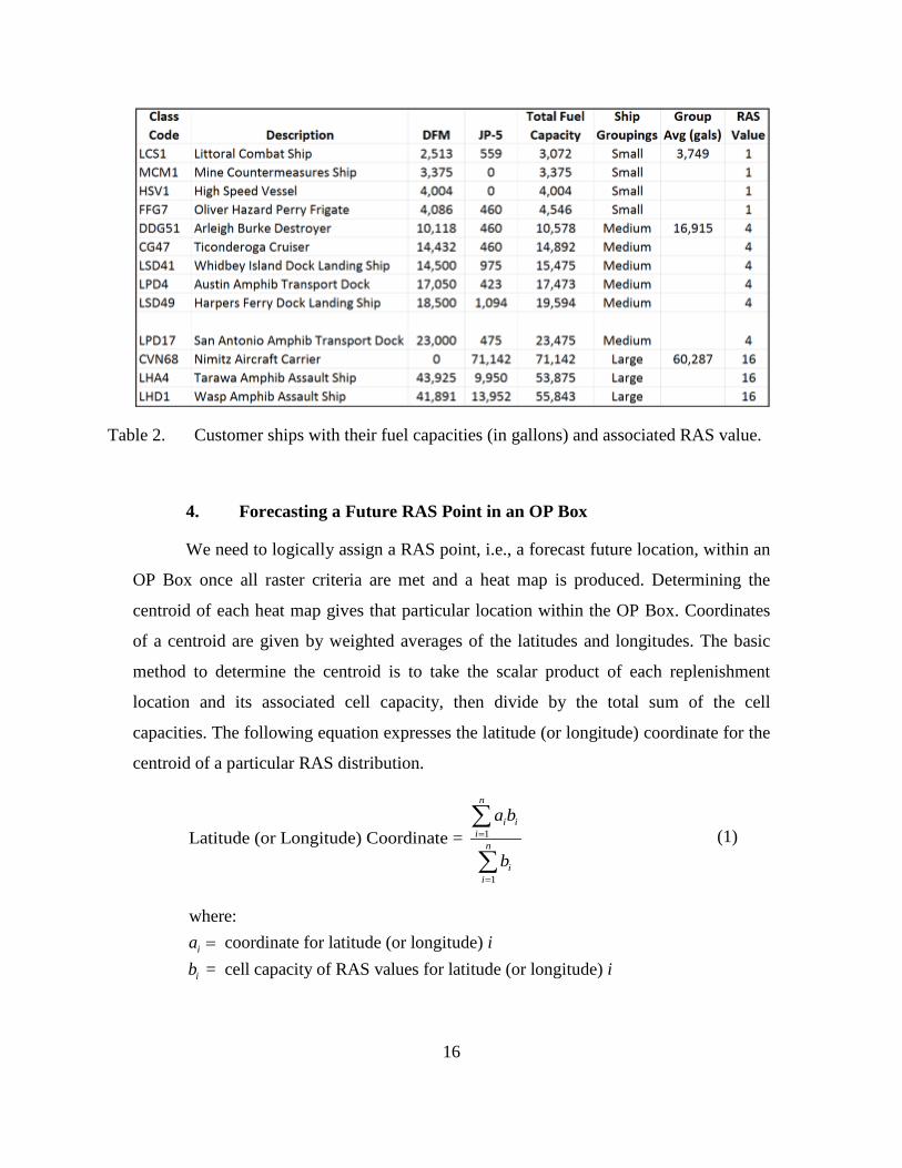
Table 2. Customer ships with their fuel capacities (in gallons) and associated RAS value. ................................................................................................................16

Table 3. Names and locations of OP Boxes for Pacific Coast Scenario. .......................17 Table 4. CentCal OP Box data set..................................................................................18 Table 5. CentCal OP Box Training Data Set. ................................................................19 Table 6. Comparison of customer readiness, fuel usage, and underway time for the

different RAS locations for the on-station Pacific Coast scenario run in RASP................................................................................................................30

Table 7. Comparison of customer readiness, fuel usage, and underway time for the RAS locations in the staggered transit Pacific Coast scenario run in RASP ...31

xii


xiii

LIST OF ACRONYMS AND ABBREVIATIONS

AME AMELIA EARHART

AO Area of Operation

BG Battle Group

BKH BUNKER HILL

CCAL Central California

CLF Combat Logistics Force

CONSOL Commodity Consolidation

CPLEX Commercial Integer Programming Solver

CTH CARTER HALL

DFM Diesel Fuel Marine

DoD Department of Defense

GAMS General Algebraic Modeling System

IB Inverted Barometer

JP-5 Jet Propellant Five

KTS Knots

MIP Mixed Integer Program

MOM MOMSEN

MSC Military Sealift Command

MXC MexiSocal

NATO North Atlantic Treaty Organization

NCAL Northern California

NM Nautical Miles

NPM Nested Process Model

xiv

OP Box Operational Area Box

ORDN Ordnance

PNW Pacific Northwest

RAS Replenishment at Sea

RASP Replenishment at-Sea Planner

STOR Subsistence Stores

T-AE Ammunition Supply Ship

T-AKE Dry Cargo/Ammunition Supply Ship

T-AO Fleet Replenishment Oiler

T-AOE Fast Combat Support Ship

UNREP Underway Replenishment

VBA Visual Basic for Applications

xv

EXECUTIVE SUMMARY

The United States Navy and its coalition partners annually consume millions of barrels of

fuel. The Combat Logistics Force (CLF) provides necessary supplies to the combatant

fleet through replenishments at sea (RAS) to sustain their missions. Furthermore, the U.S.

Navy has made a strong commitment to reducing fuel consumption due to the high cost

of oil and the constraints on government spending.

The Replenishment at-Sea Planner (RASP) is an operational planning tool that

supports the Navy’s mission of conserving fuel as it seeks optimal schedules for CLF

ships to service customers operating worldwide. RASP relies on data input of customer

positions to schedule replenishments. Planners currently forecast expected customer

positions at the geometric center of an Operational Area Box (OP Box) because there is a

deficiency of data to support more accurate location forecasts.

We introduce operational commanders who use RASP to a more accurate forecast

of future RAS locations. We begin by collecting historical replenishment events and

giving a visual representation of the data through geographical spatial heat mapping. The

heat maps we create are raster plots using the statistical computing and graphing

language, R.

From the historical RAS locations, we calculate the most probable location for a

future RAS by determining the centroid. The centroid is determined by taking the

weighted averages of each historical RAS location. The weights represent the size of

customer ships and the amounts of their demands. To verify model accuracy in

calculating the centroid, we partition our historical set of RAS events and conduct cross-

validation.

We create a fabricated scenario of the U.S. Pacific Coast that includes OP Boxes

for customer ships to operate and ports for logistical sources to CLF ships. We utilize

RASP to run our scenario. Within the scenario are geometric center points and calculated

centroids of each OP Box to which CLF ships can be routed for replenishments with

customers. We conduct separate RASP runs to produce the optimal schedules for

xvi

replenishments from geometric center and calculated centroid locations within the OP

Boxes, then compare results.

The results show that the calculated centroid location for RAS events offers

significant improvements for planning customer readiness, underway hours, and fuel

usage for CLF ships. The customer readiness and total CLF underway fuel usage are vital

performance metrics that show these differences.

xvii

ACKNOWLEDGMENTS

To my beautiful wife Cynthia, I thank God for bringing us together after so many

years of friendship. You are such a strong, loving, and supportive woman. I am amazed at

your perseverance through our studies and for that, you will always be my Superwoman.

I cannot wait for our next endeavors together and to meet our baby girl.

To Isaiah, my Little Man of Disaster, I thank you for the joy you bring into my

life. It is amazing how much you are growing before my eyes. Thank you for sacrificing

many days at the beach and train park so Mommy and Daddy could finish their thesis.

Lastly, I extend my sincere gratitude to my advisor and second reader. Professor

Brown, your patience and meticulous guidance were insurmountable. CDR DeGrange,

thank you for the countless hours of devotion in assisting me towards my completion of

this thesis. It would be an honor to serve with you out in the fleet.

xviii


1

I. INTRODUCTION

A. OVERVIEW OF COMBAT LOGISTICS FORCE

The United States Navy and its coalition partners collectively consume millions

of barrels of fuel each year as they deploy their ships throughout the world conducting

military operations ranging from peacekeeping and strategic maritime deterrence to major

combat operations. The U.S. Navy’s Military Sealift Command (MSC) encompasses a

Combat Logistics Force (CLF) that supplies the U.S. and coalition surface fleets. The

CLF is comprised of over two-dozen auxiliary ships that are grouped into four types:

Ammunition (T-AE), Dry Cargo and Ammunition (T-AKE), Fleet Replenishment Oiler

(T-AO), and Fast Combat Support (T-AOE) (MSC, 2012). Each of these ships provides

at least one component that every Navy ship requires: fuel, food, ordnance, spare parts,

mail and other supplies. The ultimate mission of the CLF is to provide reliable underway

replenishment (UNREP) to the U.S. Navy or replenishment at sea (RAS) to North

Atlantic Treaty Organization (NATO) Allies while actively supporting combat readiness

and the ability to project a powerful forward presence.

The U.S. Navy has made a strong commitment to reducing fuel consumption.

These plans are motivated by the sustained high cost of oil, the constant efforts by the

Department of Defense (DoD) to reduce government spending, and high operational

tempo for surface combatants (Early Bird article by Slavin, 2012).

During fiscal (FY) 2009, the CLF fleet spent a combined 5,036 days at sea

(Hooper, 2010). On average, every auxiliary ship is active and underway for over six

months each year. These considerations present great challenges for the Navy to reduce

its fuel consumption.

A planning tool is needed at a strategic and operational level to suggest a timely

and cost-effective way for the CLF to conduct replenishment operations for coalition

forces worldwide.

2

B. HISTORICAL RESEARCH IN CLF REPLINISHMENT PLANNING

For more than a decade, various analysts and organizations have contributed to

enhancing the CLF mission. Algorithms and models have been devised to plan and

schedule replenishment at sea (RAS) or commodity consolidation (CONSOL) throughout

areas of operation (AO) for the CLF. Efforts on this subject progressed from establishing

a simple mixed integer program (MIP) to creating dynamic optimization tools such as

Hallmann (2009) CLF Planner and Brown et al. (2010) Replenishment at-Sea Planner

(RASP). The subsequent research outlines an historical progression in establishing the

robust optimization planners to plan CLF replenishments and assess the capability and

capacity of CLF ships to support operations.

1. Initial Stages of CLF Planning

Borden (2001) gives us a first look at CLF planning through MIP. He presents

causes and effects from procuring the then-new T-AKE to conduct CLF CONSOLS and

answers fundamental questions regarding the capabilities and limitations of the T-AKE

platform in sustaining customer ships. Borden develops various scenarios that express his

questions and offers keen insight on future studies. His results reveal that a T-AKE is

incapable of maintaining transit speed with a deploying battle group (BG) at its current

load-out configuration. He recommends a plan to pre-position a forward T-AKE with the

anticipation of replenishing a fast-moving BG as it passes by, then have the T-AKE

follow the BG to its AO to be of service there.

2. Utilizing the CLF to Support Major Combat Operations and Incorporating the CLF Planning Model

Morse (2008) demonstrates an optimization model paired with a spreadsheet

interface to identify CLF requirements for campaign-level analysis through the use of a

60-day scenario. His model calculates the minimum number of CLF ships required to

sustain a large naval force conducting major theatre operations and analyzes the tradeoff

between a CLF shuttle ship versus a CLF station ship. (A shuttle ship transits between

BGs and replenishment ports, carrying commodities and transfers them via an at-sea

CONSOL event to a station ship that keeps company with the elements of the BG and in

3

turn services the on-station BG through underway replenishments (UNREP). Morse

concludes that an all-shuttle-ship concept is necessary and eliminates the need for station

ships, significantly reducing the number of CLF ships needed to support the theatre

mission.

Brown and Carlyle (2008) create a mixed integer linear program to optimize the

scheduling of all available CLF ships to service customer ships operating worldwide over

an extended planning horizon of 90–180 days. This algorithm models the delivery of four

specific commodities: Diesel Fuel Marine (DFM), Jet Propellant fuel (JP-5), dry

subsistence stores (STOR), and ordnance (ORDN). The formulation consists of seven key

types of decision variables, 14 constraint types, and applies the Floyd-Warshall algorithm

to generate the shortest paths between any two locations in a navigable sea route network.

The end result ensures that each BG maintains positive commodity inventory levels,

determines feasible CLF schedules, and optimizes the planning to best sustain all

customer ships in a given scenario. Overall, this CLF planning model has been used to

strategically deploy the CLF to support and sustain customer ships operating in theatres,

evaluate new CLF ship designs, determine the number of additional or new class of ships

needed, and demonstrate the effects of changes to naval operating policies.

Hallmann (2009) is first to meld operational planning for combatants with the

necessary planning of CLF activities to support such plans. His work reinforces its

reliability as a practical decision-making tool to fleet and theatre commanders as he

employed the planning tool during a Fleet Forces exercise TRIDENT WARRIOR 2009

that allowed planners to calculate optimal CLF schedules through predetermined time

horizons. This exercise consisted of scenarios that generated MIPs with about 5,500

constraints and 6,000 variables, of which 1,200 are binary. Using the General Algebraic

Modeling System (GAMS) and the commercial integer programming solver (CPLEX)

(GAMS, 2012), solution runtimes typically ranged from 5 to 10 minutes based on the

level of complexity of the scenarios. This CLF Planner provides time and flexibility for

commanders to make more methodical decisions in planning, scheduling, and executing

the employment of the logistics force.

4

3. Revolutionizing CLF Planning into an Operational Model

The original CLF planning model is designed as a strategic decision aid that

studies the influence of composition and employment of logistics forces and their

resulting ability to support combat ships throughout worldwide operations. The

complexities of scheduling these operations are of major focus at the Chief of Naval

Operations Strategic Mobility and Combat Logistics Division, also known as OPNAV

N42. In addition, MSC and Theatre Task Force Commanders have further inquired about

evolving the model to account for planning at the operational level.

Brown et al. (2010) formulate a completely revised model from the legacy CLF

planner. Contrary to its predecessor, the Replenishment At Sea Planner (RASP) accounts

for higher time fidelity at the request of MSC and theatre commanders in order to meet

their operational needs. The shorter increments of time and the key concept of a shuttle-

ship leg enables RASP to account for speed requirements, fuel consumption, and reduce

costs. For more insight on RASP, refer to Brown et al. (2010).

C. DEFICIENCY OF DATA SUPPORTING RASP

Although operational-level CLF planning has evolved immensely since Brown et

al. introduced RASP, there is still room for continued improvement for replenishment

scheduling by refining data inputs provided to the model. UNREP planning is heavily

utilized through RASP at the operational level and MSC is most interested in the

continued development of the model. Additionally, Commander Task Force 53 (CTF-53)

and potentially other task force commanders are captivated with the notion that RASP

can be utilized as a viable and robust asset to optimally plan and track replenishments

during real-world major operations in various theatres. However, there are still factors

that make commanders reluctant to fully incorporate the model in their operations.

The downside of RASP is that the model must rely on forecast combatant

locations to plan replenishments and there is no analysis to support these locations. For

an operator, it is important to have an accurate representation of where replenishments

can occur, and utilize them in the model.

5

By definition, replenishments occur between two ships either in port or at sea.

Because we are only focusing on at-sea replenishments between two ships, the terms

RAS and CONSOL will be used interchangeably. Moreover, RAS and UNREP will be

synonymous as we will neglect to distinguish between replenishing with U.S. only and

NATO allies.

For every RAS that the optimal solution suggests in a given scenario, there is an

associated rendezvous position for a customer and CLF ship to conduct the

replenishment. These positions are defined by planner input to the model. The center of a

specified Operational Area Box (OP Box) is the current RAS position. In most cases, the

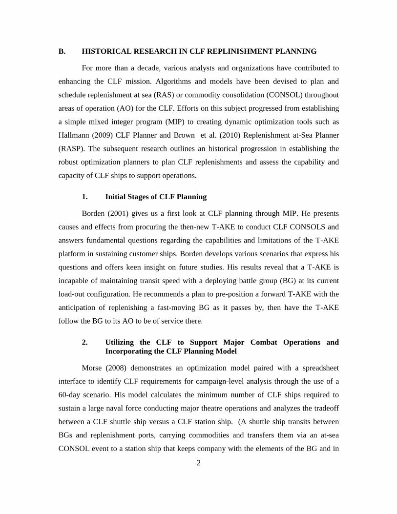
assigned location of replenishments can be far from where they actually take place.

In many instances, a CLF ship may be scheduled to go farther or shorter than

necessary to rendezvous for a RAS as the designated location does not reflect an accurate

forecast of customer positions. Depending on the size of the OP Box, this error could

produce drastic effects in productivity. Figure 1 gives a possible scenario from RASP

where a CONSOL is assigned in the center of an OP Box.

Figure 1. A CLF ship enters the OP Box from the top right corner, transits to center to conduct a RAS at the designated location, and then transits back out of OP Box to

its previous entry location.

6

Given the OP Box dimensions of 1x1 day transit time and using the Pythagorean

Theorem, it would take a CLF ship at least 1.4 days of total transit time to replenish a

ship and return to place of origin. If historical data shows that the tendency for ships were

to UNREP in the upper right (North-East) corner in the OP Box, it would not make sense

to continuously schedule the CLF ship to the center for CONSOLS. If the RAS point was

modified towards the more-frequented area for UNREPs, it would better reflect the true

location and could possibly enhance the optimality of RASP suggestions.

RASP needs better forecasted positions for replenishments rather than the default

input assignment of a RAS to the center of the OP Box. Having the replenishment

locations properly altered could reduce planned transit time, cost, and ultimately present a

true measure of optimality in a given scenario.

D. DEVELOPING A MORE ACCURATE MODEL TO FORECAST REPLENISHMENT LOCATIONS

The purpose of this thesis is to provide operational commanders using RASP

more accurate forecasts of future replenishment locations. We begin by using historical

replenishment locations and develop a way to predict future RAS locations. These

historical RAS locations will be mapped to reckon where future ones will take place.

We present geographical spatial mapping that creates a visual reference and

representation of the distribution of the historical RAS locations. It will consist of

quantifiable data and be displayed through multiple colors, commonly referred to as heat

mapping.

The mapping will display the frequency and location of CONSOL events that

have taken place within a given operating area. With these frequencies, we will analyze

the historical data and determine the most logical location to forecast a future RAS. And

through our results, we verify the validity of our forecast RAS location, conduct

comparative analysis with the default RAS input of assignments into RASP, and

determine impact on CLF customer readiness, underway hours, fuel, and cost.

7

II. HEAT MAP LITERATURE REVIEW

A. THE ORIGIN OF THE HEAT MAP

A heat map is a two-dimensional graphical representation of data that is

represented by colors (Wilkinson, 2004). The heart of the heat map is a color-shaded

matrix display of data. Data has been displayed in shaded matrix form for well over a

century, dating back to Loua’s (1873) hand-drawn and colored graphics of social

statistics across the administrative districts of Paris.

B. HEAT MAPPING TYPES

There are multiple ways to display a heat map; they range from the business

process “tree mapping diagram” (shown in Figure 2) to statistical methods in producing a

spatial-temporal map (shown in Figure 3). We will use spatial mapping. Spatial mapping

consists of geographical data that is referenced to a map projection on the earth

coordinate system (ESRI, 2012). Spatial mapping is most commonly displayed in clusters

or raster objects.

Figure 2. A Business Tree Map. (Available from http://www.smartmoney.com, 2012). This is a snapshot of the stock market after closing on August 14, 2012. Boxes represent companies nested under a listed industry. Size of box is directly proportional to the size of their respective market capitalization. Boxes are colored based upon percentage gain (green or lighter shaded) or loss (red or darker shaded).

8

Figure 3. A Spatio-Temporal Map. (From Cressie and Wikle, 2011). This is a Hierarchical Dynamic Spatio-Temporal Mapping of sea surface temperature anomalies for October 1997 (left column) and October 1998 (right column). The color scale depicts the above or below average temperature (in degrees Celsius) for the spatial data.

1. Cluster Mapping

Wilkinson and Friendly (2009) describe the cluster heat map as a crafty way to

display row- and column-categorized clustered data in matrix form. MicroImages’

Scientific Writers (2012) defines cluster mapping as the process in which multiple

overlapping layers are reduced to a single raster display. The rasters used in clustering

can represent multiple data.

2. Raster Plotting

A raster or raster object consists of one or more images or grids that represent a

layer in two-dimensional form. It contains a grouped set of numbers from a single data

type, where each number represents the value of a given parameter. (MicroImages’

Scientific Writers, 2012)

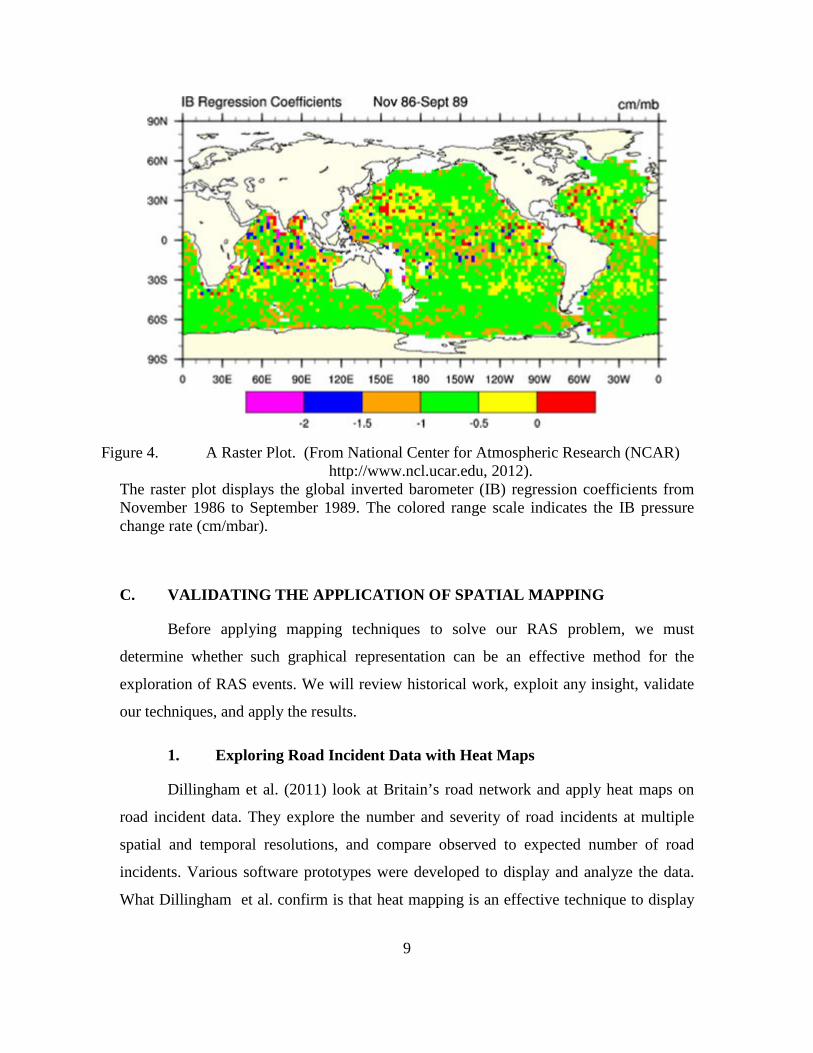
Hijmans (2012) describes a raster as a spatial data structure that divides a

particular region into grid-like cells, in which each cell can store one or more values.

Figure 4 is an example that depicts Hijman’s raster description.

9

Figure 4. A Raster Plot. (From National Center for Atmospheric Research (NCAR) http://www.ncl.ucar.edu, 2012).

The raster plot displays the global inverted barometer (IB) regression coefficients from November 1986 to September 1989. The colored range scale indicates the IB pressure change rate (cm/mbar).

C. VALIDATING THE APPLICATION OF SPATIAL MAPPING

Before applying mapping techniques to solve our RAS problem, we must

determine whether such graphical representation can be an effective method for the

exploration of RAS events. We will review historical work, exploit any insight, validate

our techniques, and apply the results.

1. Exploring Road Incident Data with Heat Maps

Dillingham et al. (2011) look at Britain’s road network and apply heat maps on

road incident data. They explore the number and severity of road incidents at multiple

spatial and temporal resolutions, and compare observed to expected number of road

incidents. Various software prototypes were developed to display and analyze the data.

What Dillingham et al. confirm is that heat mapping is an effective technique to display

10

the data. They determine this through two evaluation methods; one being Munzner’s

(2009) Nested Process Model (NPM).

2. The Nested Process Model (NPM)

To determine whether heat mapping is an effective technique, it is essential to

demonstrate that a heat map is appropriate for the task and is well constructed to

demonstrate the technique’s validity (Munzner, 2009). The NPM, shown in Figure 5, is a

visualization design and validation technique that uses four cascading layers:

• Characterize the task and data of the problem domain,

• Abstract into operations and data types,

• Design visual encoding and interaction techniques, and

• Create algorithms to execute techniques efficiently.

Figure 5. The four-layer Nested Model. (From Munzner, 2009).

Munzner also provides a structure within which the factors threatening heat

mapping’s validity can be examined, shown in Figure 6.

11

Figure 6. Threats and validation in the nested model. (From Munzner, 2009).

The first two steps seem trivial because our RAS problem is similar to

Dillingham’s et al. (2011) road incident network. We can also manipulate our data to

eliminate any threats at step two. In seeking to assess the effectiveness of heat mapping,

we will primarily focus on levels three and four of the NPM; designing visual encoding

and interaction techniques and creating algorithms to execute techniques efficiently.

12


13

III. SPATIAL MAP AND CENTROID ALGORITHM

We display the spatial maps in generic, clustered form using raster plotting with

the statistical computing and graphing language, R (R Core Team, 2012). R is an open-

source programming language that enables us to create an algorithm to produce our heat

maps efficiently.

A. DISTRIBUTIONS OF HISTORICAL REPLENISHMENTS

Historical replenishment locations can occur in various distribution types within a

given area. The distributions are influenced by geographical area and operational

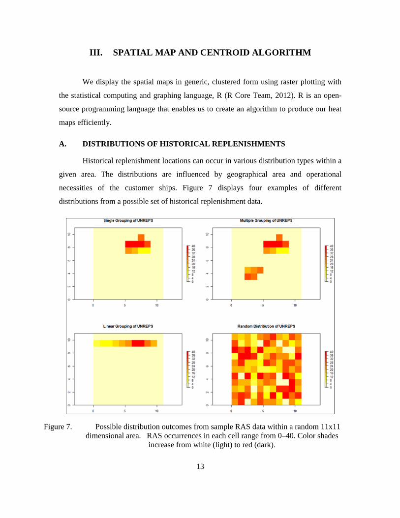
necessities of the customer ships. Figure 7 displays four examples of different

distributions from a possible set of historical replenishment data.

Figure 7. Possible distribution outcomes from sample RAS data within a random 11x11 dimensional area. RAS occurrences in each cell range from 0–40. Color shades

increase from white (light) to red (dark).

14

B. BUSINESS RULES FOR DESIGNING RASTER PLOTS

Raster plots have many elements that allow us to graphically express RAS data.

We implement business rules in order to effectively design our raster plots and determine

a most-likely future replenishment position. The key components that enable us to

identify and outline these rules are size, location, and values within the OP Boxes.

1. Dimensions of an OP Box

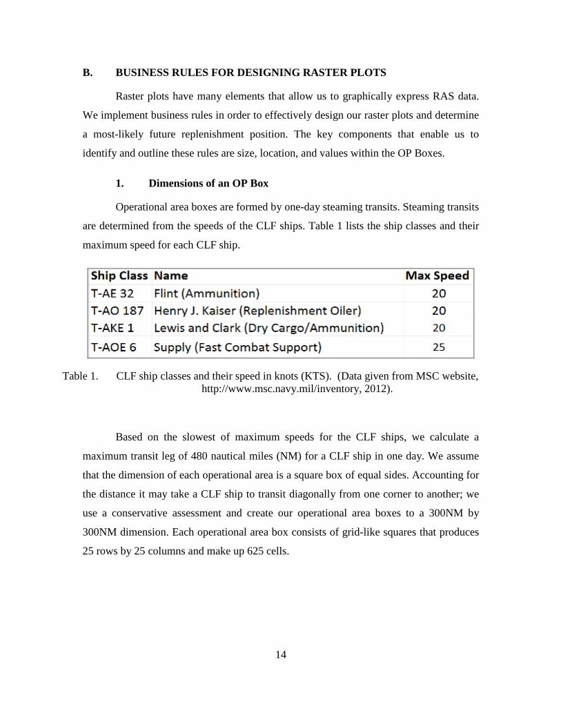
Operational area boxes are formed by one-day steaming transits. Steaming transits

are determined from the speeds of the CLF ships. Table 1 lists the ship classes and their

maximum speed for each CLF ship.

Table 1. CLF ship classes and their speed in knots (KTS). (Data given from MSC website, http://www.msc.navy.mil/inventory, 2012).

Based on the slowest of maximum speeds for the CLF ships, we calculate a

maximum transit leg of 480 nautical miles (NM) for a CLF ship in one day. We assume

that the dimension of each operational area is a square box of equal sides. Accounting for

the distance it may take a CLF ship to transit diagonally from one corner to another; we

use a conservative assessment and create our operational area boxes to a 300NM by

300NM dimension. Each operational area box consists of grid-like squares that produces

25 rows by 25 columns and make up 625 cells.

15

2. Creating Geographical Raster Plots

a. Coordinate Referencing System

The default coordinate referencing system for raster plots in R is the

World Geodetic System 84 (WGS-84) datum (R Core Team, 2012). We use this common

reference system to plot our rasters on a map. The x-axis represents latitude values and

the y-axis represents longitude values. Valid coordinate entries are in decimal form with a

negative number representing West-or-South and positive representing East-or-North.

b. Correlating Geographic Locations to Raster Cells

Every raster cell covers a 0.2 degree latitude and longitude area, and

contains some numerical value representing activity there.

c. Distortions From Map Projection

Geographic distortions occur as a result of using any type of map

projection. For our case, the raster cells become narrower in width (longitude) as we

approach either pole.

3. Cell Values and Weightings

Each cell contains the frequency of replenishments occurring therein. The total

frequency in each cell is identified as the cell capacity. Each cell may have multiple RAS

events that make up the cell capacity. Additionally, replenishments are not a one-for-one

value; they are weighted differently and dependent upon each customer ship.

A customer ship is assigned to one of three groupings that represent its numerical

value for a single RAS event. Groupings are determined by comparative combined fuel

capacities of the ships. Each grouping has an associated RAS value calculated from the

weighted average relative to their counterparts. Customer ships, their associated

groupings, and RAS values are given in Table 2.

16

Table 2. Customer ships with their fuel capacities (in gallons) and associated RAS value.

4. Forecasting a Future RAS Point in an OP Box

We need to logically assign a RAS point, i.e., a forecast future location, within an

OP Box once all raster criteria are met and a heat map is produced. Determining the

centroid of each heat map gives that particular location within the OP Box. Coordinates

of a centroid are given by weighted averages of the latitudes and longitudes. The basic

method to determine the centroid is to take the scalar product of each replenishment

location and its associated cell capacity, then divide by the total sum of the cell

capacities. The following equation expresses the latitude (or longitude) coordinate for the

centroid of a particular RAS distribution.

1

1

Latitude (or Longitude) Coordinate =

n

i ii

n

ii

a b

b

=

=

∑

∑ (1)

where: coordinate for latitude (or longitude)

= cell capacity of RAS values for latitude (or longitude) i

i

a ib i=

17

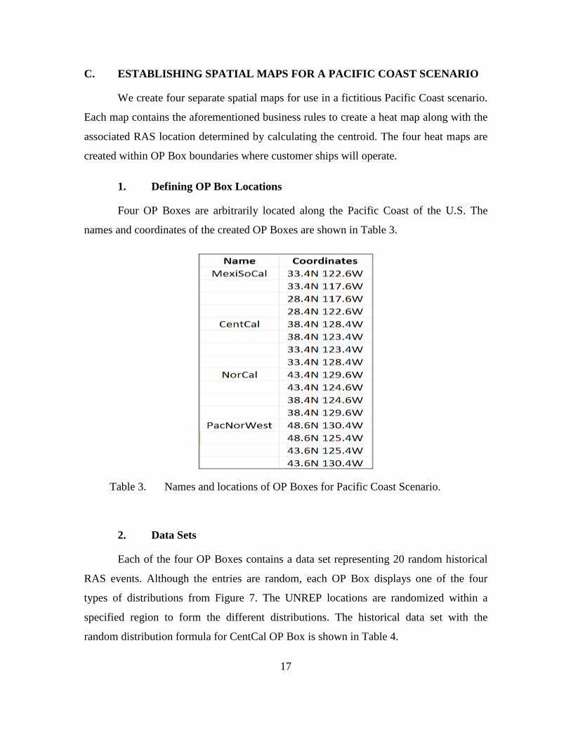
C. ESTABLISHING SPATIAL MAPS FOR A PACIFIC COAST SCENARIO

We create four separate spatial maps for use in a fictitious Pacific Coast scenario.

Each map contains the aforementioned business rules to create a heat map along with the

associated RAS location determined by calculating the centroid. The four heat maps are

created within OP Box boundaries where customer ships will operate.

1. Defining OP Box Locations

Four OP Boxes are arbitrarily located along the Pacific Coast of the U.S. The

names and coordinates of the created OP Boxes are shown in Table 3.

Table 3. Names and locations of OP Boxes for Pacific Coast Scenario.

2. Data Sets

Each of the four OP Boxes contains a data set representing 20 random historical

RAS events. Although the entries are random, each OP Box displays one of the four

types of distributions from Figure 7. The UNREP locations are randomized within a

specified region to form the different distributions. The historical data set with the

random distribution formula for CentCal OP Box is shown in Table 4.

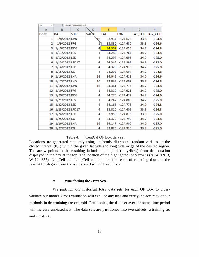
18

Table 4. CentCal OP Box data set. Locations are generated randomly using uniformly distributed random variates on the closed interval (0,1) within the given latitude and longitude range of the desired region. The arrow points to the resulting latitude highlighted (in yellow) from the equation displayed in the box at the top. The location of the highlighted RAS row is (N 34.30913, W 124.655). Lat_Cell and Lon_Cell columns are the result of rounding down to the nearest 0.2 degree from the respective Lat and Lon entries.

a. Partitioning the Data Sets

We partition our historical RAS data sets for each OP Box to cross-

validate our model. Cross-validation will exclude any bias and verify the accuracy of our

methods in determining the centroid. Partitioning the data set over the same time period

will increase unbiasedness. The data sets are partitioned into two subsets; a training set

and a test set.

19

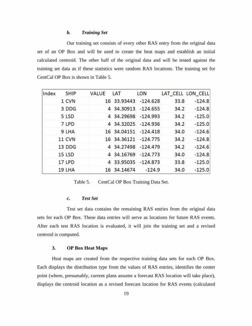
b. Training Set

Our training set consists of every other RAS entry from the original data

set of an OP Box and will be used to create the heat maps and establish an initial

calculated centroid. The other half of the original data and will be tested against the

training set data as if these statistics were random RAS locations. The training set for

CentCal OP Box is shown in Table 5.

Table 5. CentCal OP Box Training Data Set.

c. Test Set

Test set data contains the remaining RAS entries from the original data

sets for each OP Box. These data entries will serve as locations for future RAS events.

After each test RAS location is evaluated, it will join the training set and a revised

centroid is computed.

3. OP Box Heat Maps

Heat maps are created from the respective training data sets for each OP Box.

Each displays the distribution type from the values of RAS entries, identifies the center

point (where, presumably, current plans assume a forecast RAS location will take place),

displays the centroid location as a revised forecast location for RAS events (calculated

20

from the historical data and formulation expressed in equation 1), and returns the distance

between the OP Box center point and the centroid. Figures 8–11 show the heat maps for

the four different OP Box regions.

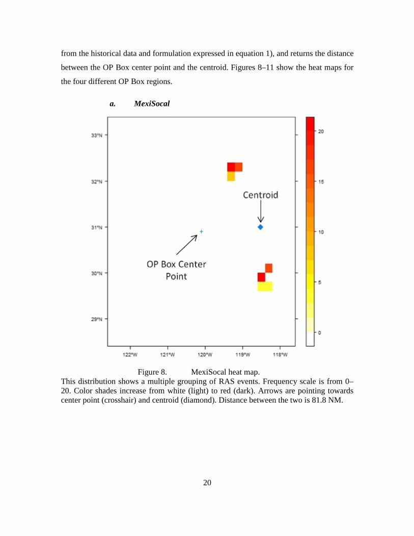
a. MexiSocal

Figure 8. MexiSocal heat map. This distribution shows a multiple grouping of RAS events. Frequency scale is from 0–20. Color shades increase from white (light) to red (dark). Arrows are pointing towards center point (crosshair) and centroid (diamond). Distance between the two is 81.8 NM.

21

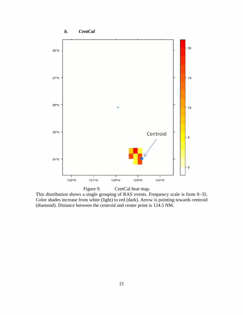
b. CentCal

Figure 9. CentCal heat map. This distribution shows a single grouping of RAS events. Frequency scale is from 0–35. Color shades increase from white (light) to red (dark). Arrow is pointing towards centroid (diamond). Distance between the centroid and center point is 124.5 NM.

22

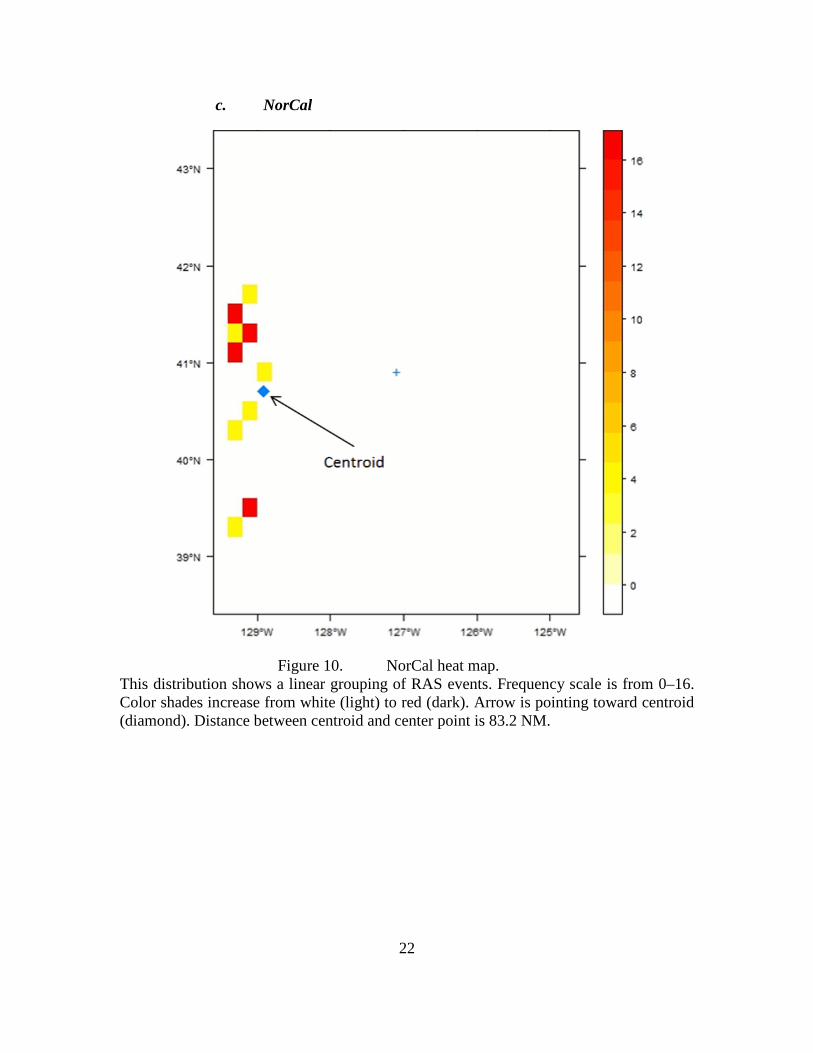
c. NorCal

Figure 10. NorCal heat map. This distribution shows a linear grouping of RAS events. Frequency scale is from 0–16. Color shades increase from white (light) to red (dark). Arrow is pointing toward centroid (diamond). Distance between centroid and center point is 83.2 NM.

23

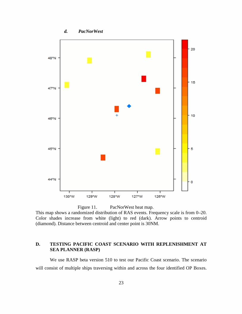
d. PacNorWest

Figure 11. PacNorWest heat map. This map shows a randomized distribution of RAS events. Frequency scale is from 0–20. Color shades increase from white (light) to red (dark). Arrow points to centroid (diamond). Distance between centroid and center point is 30NM.

D. TESTING PACIFIC COAST SCENARIO WITH REPLENISHMENT AT SEA PLANNER (RASP)

We use RASP beta version 510 to test our Pacific Coast scenario. The scenario

will consist of multiple ships traversing within and across the four identified OP Boxes.

24

A RAS schedule will be developed using the geometric center point as well as using the

centroid from historical UNREPS for RAS locations. The results will then be analyzed.

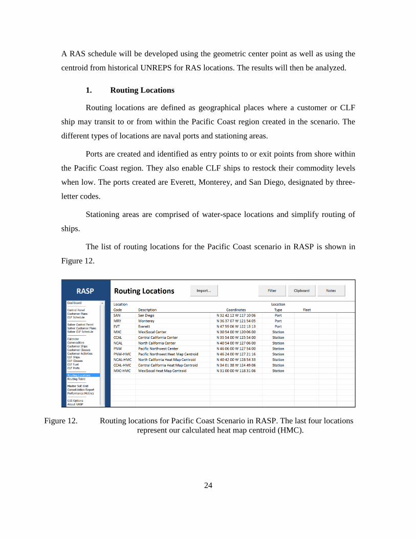
1. Routing Locations

Routing locations are defined as geographical places where a customer or CLF

ship may transit to or from within the Pacific Coast region created in the scenario. The

different types of locations are naval ports and stationing areas.

Ports are created and identified as entry points to or exit points from shore within

the Pacific Coast region. They also enable CLF ships to restock their commodity levels

when low. The ports created are Everett, Monterey, and San Diego, designated by three-

letter codes.

Stationing areas are comprised of water-space locations and simplify routing of

ships.

The list of routing locations for the Pacific Coast scenario in RASP is shown in

Figure 12.

Figure 12. Routing locations for Pacific Coast Scenario in RASP. The last four locations represent our calculated heat map centroid (HMC).

25

2. Ships

The customer ship schedules are arbitrary, but held constant between the RAS

geometric center location and the calculated centroid location for both scenario runs.

Upon commencement of each scenario run, the commodity levels for all customer ships

are at 80% full, while CLF ships will are at (100%) full commodity.

a. Ship Tracks

RAS input consist of locations and times. RASP interpolates them period-

by-period. When RASP interpolates transit locations period-by-period, it creates

intermediate points between points and station positions. RAS events may be scheduled

at such intermediate points.

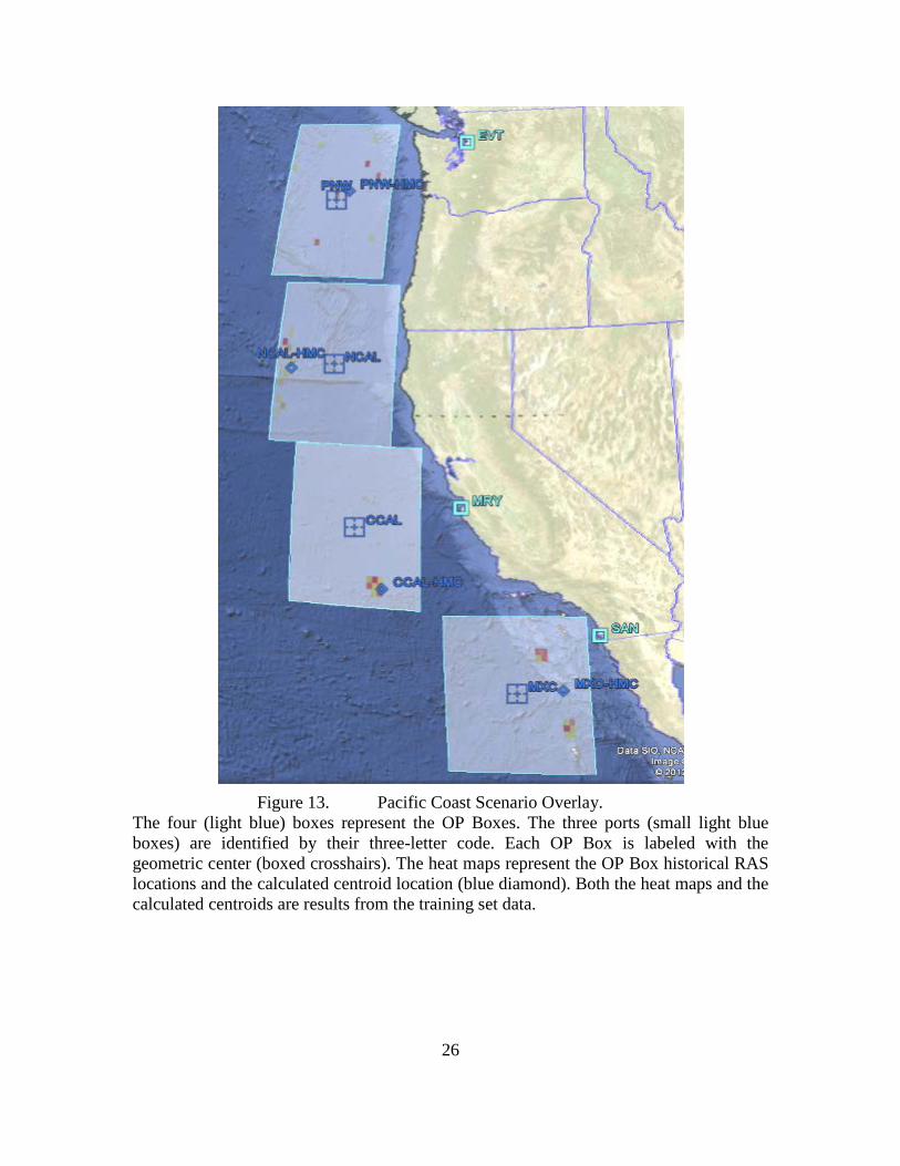
3. Scenario Overlay

Figure 13 gives a combined overlaid look of the Pacific Coast scenario that

includes the heat maps, centroids, and center points for each OP Box.

26

Figure 13. Pacific Coast Scenario Overlay.

The four (light blue) boxes represent the OP Boxes. The three ports (small light blue boxes) are identified by their three-letter code. Each OP Box is labeled with the geometric center (boxed crosshairs). The heat maps represent the OP Box historical RAS locations and the calculated centroid location (blue diamond). Both the heat maps and the calculated centroids are results from the training set data.

27

IV. ANALYSIS AND CONCLUSIONS

The insights we wish to acquire in this analysis are twofold. The first is to verify

that our centroid is an improvement. This will determine whether our centroids for each

OP Box are logical locations that represent the RAS and operating areas of customer

ships. The second is to determine if there is any significant difference in the RASP

schedules between the default geometric center of the OP Box and the centroid location.

We focus on the variations in customer readiness and CLF fuel usage.

A. CROSS-VALIDATION OF CENTROIDS

We use cross-validation to estimate how accurate our calculated centroids are

with test data RAS locations by calculating a new centroid using RAS locations from

each test set event. The centroid will change as additional RAS events take place from the

test data set. Using this relationship we can compare the initial centroid from the training

set data with the calculated centroids and calculate the distances through each subsequent

RAS in the test set.

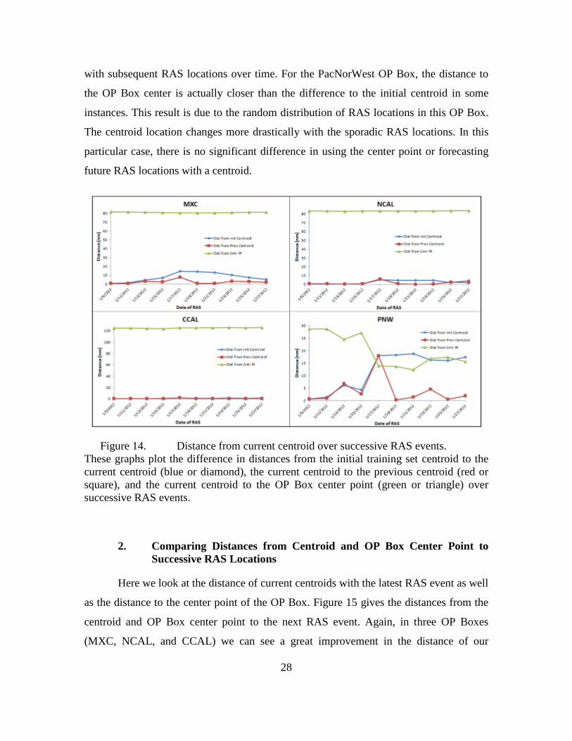
1. Comparing Distances from Current Centroid over Time

Part of our validation involves taking the difference of the distance between

centroids over time and comparing it to the distance from the center point of an OP Box.

We use the test data set to produce new RAS events. We then calculate three distances

from the updated centroid and compare differences: the distance from current centroid to

previous centroid, the current to initial centroid, and current to the center point.

Figure 14 displays distances from the current centroid over successive RAS event

for each OP Box. We can see from this figure how the centroid changes with additional

RAS events over time and how it compares with the distance to the center point. In three

of the four OP Boxes (MXC, NCAL, and CCAL), the distance of the current centroid in

relation to initial and previous centroids is significantly and consistently smaller than the

distance to the OP Box center. This shows that the centroid locations are an improvement

from the center points of those OP Boxes as they better represent and closely associate

28

with subsequent RAS locations over time. For the PacNorWest OP Box, the distance to

the OP Box center is actually closer than the difference to the initial centroid in some

instances. This result is due to the random distribution of RAS locations in this OP Box.

The centroid location changes more drastically with the sporadic RAS locations. In this

particular case, there is no significant difference in using the center point or forecasting

future RAS locations with a centroid.

Figure 14. Distance from current centroid over successive RAS events. These graphs plot the difference in distances from the initial training set centroid to the current centroid (blue or diamond), the current centroid to the previous centroid (red or square), and the current centroid to the OP Box center point (green or triangle) over successive RAS events.

2. Comparing Distances from Centroid and OP Box Center Point to Successive RAS Locations

Here we look at the distance of current centroids with the latest RAS event as well

as the distance to the center point of the OP Box. Figure 15 gives the distances from the

centroid and OP Box center point to the next RAS event. Again, in three OP Boxes

(MXC, NCAL, and CCAL) we can see a great improvement in the distance of our

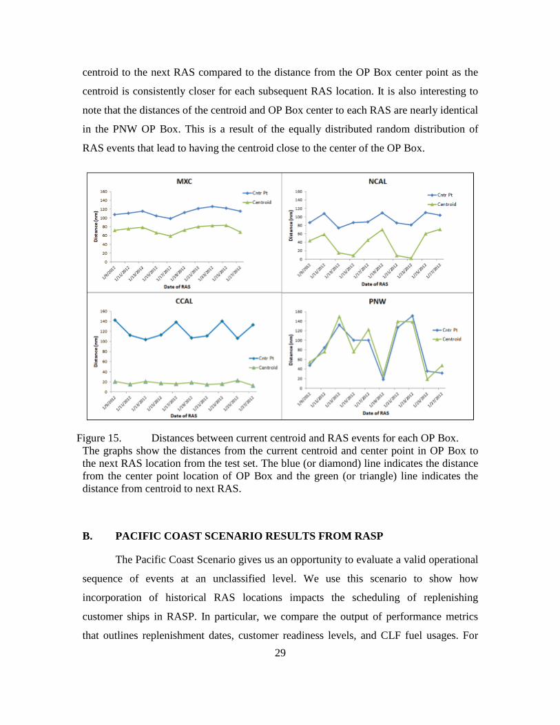
29

centroid to the next RAS compared to the distance from the OP Box center point as the

centroid is consistently closer for each subsequent RAS location. It is also interesting to

note that the distances of the centroid and OP Box center to each RAS are nearly identical

in the PNW OP Box. This is a result of the equally distributed random distribution of

RAS events that lead to having the centroid close to the center of the OP Box.

Figure 15. Distances between current centroid and RAS events for each OP Box. The graphs show the distances from the current centroid and center point in OP Box to the next RAS location from the test set. The blue (or diamond) line indicates the distance from the center point location of OP Box and the green (or triangle) line indicates the distance from centroid to next RAS.

B. PACIFIC COAST SCENARIO RESULTS FROM RASP

The Pacific Coast Scenario gives us an opportunity to evaluate a valid operational

sequence of events at an unclassified level. We use this scenario to show how

incorporation of historical RAS locations impacts the scheduling of replenishing

customer ships in RASP. In particular, we compare the output of performance metrics

that outlines replenishment dates, customer readiness levels, and CLF fuel usages. For

30

better illustration, we provide two different situations and outcomes; ships on station in

OP Boxes and ships transiting through OP Boxes.

1. Ships on Station in MXC and CCAL

For this run we use two customer ships USS MOMSEN (MOM) and USS

CARTER HALL (CTH) and a TAK-E USNS AMELIA EARHART (AME). MOM and

CTH are operating in CCAL and MXC OP Boxes respectively. We run RASP with a 15-

day solve for both the center-point RAS location run and the centroid RAS location run.

Refer to Appendix A for a detailed schedule and comparison of the solver customer plans

for this scenario.

Table 6 displays the results of the two on-station runs and gives comparison from

the RASP performance metrics worksheet (a standard output of RASP). Because the

centroids are closer to San Diego port entry for both OP Boxes than their OP Box center

points, the CLF alters CONSOL movements as the optimality of the two scenarios

differs. The optimal solution for the centroid run results in AME delaying its transit to

replenish MOM in the CCAL region while first replenishing CTH in MXC.

The centroid run gives a increased customer readiness and expends less fuel from

CLF. AME expends nearly 21,000 gallons more in fuel and over two extra days

underway in the center point scenario. With an estimate of a barrel of oil at $116, the

Navy would consume over $58K in excess costs of fuel in this 15-day scenario.

Table 6. Comparison of customer readiness, fuel usage, and underway time for the different RAS locations for the on-station Pacific Coast scenario run in RASP.

Data is taken from the results in the RASP 510 performance metrics worksheet. The above safety stock, below safety stock, and below extremis stock fields are shown in the left, middle (orange), and right (red) columns respectively under customer readiness. The default RAS run has a lower customer readiness level while the centroid RAS run has no customer hitting extremis, lower fuel expenditure, and less underway time.

31

2. Group of Ships Transiting from PNW to MXC

This scenario contains three customer ships MOM, CTH and USS BUNKER

HILL (BKH) with a TAK-E (AME) and TAO-E (USNS RAINIER). The three customer

ships are on staggered transits over a 15-day period to MXC OP Box with a starting

location in PNW. Refer to Appendix B for a detailed schedule and comparison of the

solver customer plans for this scenario.

Table 7 displays the results of the two staggered transit runs and gives comparison

from the RASP performance metrics worksheet. Significant differences between

customer readiness from the optimal solutions occur when AME manages to replenish

BKH in NCAL from the center-point run while the centroid run allows her to remain

below safety stock at end of the 15-day window. The factor here is that the NCAL-HMC

is further west and away from all ports than the center point of NCAL.

The customer readiness levels for the centroid run shows more degradation as

ships only remain above safety stock 73% of the time as opposed to 86% in the center-

point run. However, the CLF still manages to expend less fuel and underway hours in the

centroid run.

Table 7. Comparison of customer readiness, fuel usage, and underway time for the RAS locations in the staggered transit Pacific Coast scenario run in RASP

The resulting numbers from the optimal solutions of the two runs can be a bit

misleading. The center-point RAS scenario schedule contains an additional replenishment

that accounts for the extra fuel and underway time expenditures. The results from the

center-point run reflect a more accurate picture of the logistical scheduling.

As we can see, the two different RAS locations (center point and centroid)

produce significant differences in schedules and CLF performance. And regardless of the

32

outcome of each run in a scenario, we must focus on the centroid RAS location due to the

fact of better forecasting customer positions.

C. CONCLUSION

1. Summary

Military operational planners should be keenly aware of the importance of using

historical RAS locations for accurate logistical planning of the future. RASP can provide

planners optimal schedules for CLF ships but relies on input data. Determining estimated

RAS locations from historical data will give better input into RASP.

The heat map and the RAS calculated centroid technique utilizes historical data to

provide a more accurate input into RASP. The model determines the most probable RAS

location given the distribution of historical data. Planning for RAS events at the centroid

rather than at the center point location will result in an increase in planning accuracy and

a more effective use of CLF assets.

2. Recommendations for Future Research

a. Creating Scenario on Actual Historical Data

Due to the classification of utilizing actual RAS locations, we are unable

to run a scenario on real historical replenishment data. Spatial mapping and this centroid

process can be used in a classified setting to analyze RAS locations in current areas of

naval operations.

b. Include Exponential Weighting in Assigning Values of RAS Events

One can include an additional exponentially weighting variable based on

RAS event dates. This type of weighting would allow the most recent RAS event

locations to influence the centroid location to a greater extent.

33

c. Predicting Future RAS Locations through Time Series Analysis

Forecasting future RAS locations can be done using time series analysis.

One could predict where the next RAS location will occur using moving averages from

the historical data. Results of this study can be compared to the results of the centroid

technique introduced here.

d. Interfacing a Heat Map and Centroid Method into RASP

RASP is a powerful logistical planning tool and its features are constantly

improving to cater to the needs of the planers. Incorporating heat maps and centroids

through Microsoft Excel’s Visual Basic for Applications (VBA) coding and interfacing

into the map dashboard of RASP will give the planner a historical perspective of

logistically supported RAS locations.

34


35

APPENDIX A. SOLVER CUSTOMER PLANS COMPARISON OF ON-STATION RASP RUN

The following figures display the customer plans produced from the RAS

locations at the center point of the OP Boxes (first figure) and the centroid of the OP

Boxes (second figure) of the on-station run in RASP. The last four columns of each

figure indicate the daily commodity levels for the respective ship. Yellow indicates that a

ship will fall below safety stock for that particular commodity level. Red indicates that

the ship will fall below extremis stock for that particular commodity level. For example,

in the center-point RAS (first figure), the CARTER HALL falls below safety stock in

DFM, JP-5, dry stores and cargo, and chilled stores on 07 Jan, 04 Jan, 11 Jan, and 10 Jan

respectively. She also falls below extremis stock in JP-5 on 11 Jan.

Screen shot from Replenishment at Sea Planner RASP showing state of customer ships over planning horizon.

36


37

APPENDIX B. SOLVER CUSTOMER PLANS COMPARISON OF STAGGERED TRANSIT RASP RUN

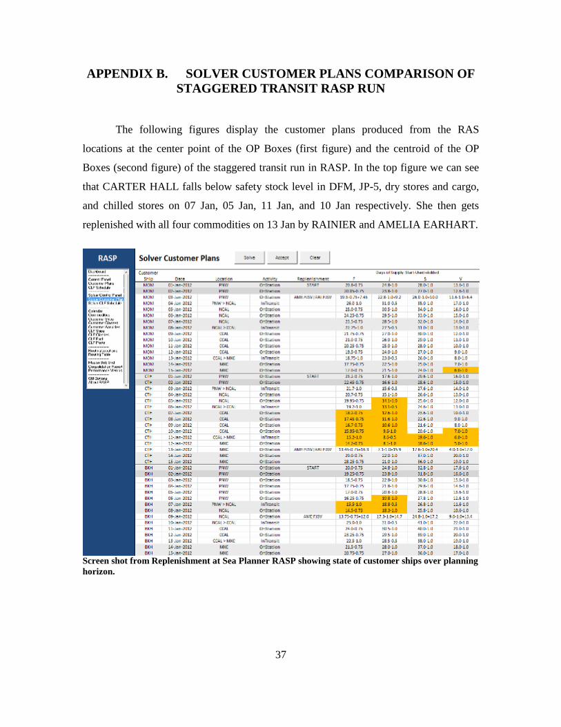
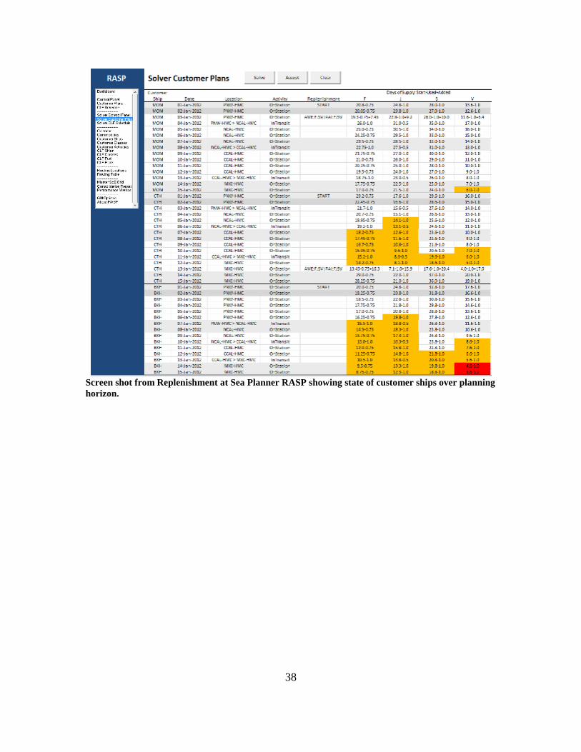
The following figures display the customer plans produced from the RAS

locations at the center point of the OP Boxes (first figure) and the centroid of the OP

Boxes (second figure) of the staggered transit run in RASP. In the top figure we can see

that CARTER HALL falls below safety stock level in DFM, JP-5, dry stores and cargo,

and chilled stores on 07 Jan, 05 Jan, 11 Jan, and 10 Jan respectively. She then gets

replenished with all four commodities on 13 Jan by RAINIER and AMELIA EARHART.


38


39

LIST OF REFERENCES

Borden, K. D., 2001, “Optimizing the Number and Employment Combat Logistics Force Shuttle Ships, with a Case Study of the New T-AKE Ship,” MS Thesis in Operations Research, Naval Postgraduate School, September.

Brown, G.G. and Carlyle, M.W., 2008, “Optimizing the U.S. Navy’s Combat Logistics Force,” Naval Research Logistics, 55 (8), pp. 800–810.

Brown, G.G., Carlyle, M.W., and Burson, P., 2010, “Replenishment at Sea Planner (RASP) Model,” Operations Research Department, Naval Postgraduate School, Monterey, July.

Cressie, N. and Wilke, C., 2011, Statistics for Spatio-Temporal Data. Hoboken, New Jersey: John Wiley & sons, Inc.

Dillingham, ., Mills, B., and Dykes, J., 2011, “Exploring Road Incident Data with Heat Maps.” Geographic Information Science Research UK, University of Portsmouth, Portsmouth, UK, retrieved May 29, 2012 from http://openacess.city.ac.uk.

Environmental Systems Research Institute (ESRI), 2012, Geographic Information System, last accessed July 15, 2012 from http://www.esri.com.

GAMS, 2012, General Algebraic Modeling System Development Corporation (User Guide), last accessed July 5, 2012 from http://www.gams.com.

Hallmann, F., 2009, “Optimizing Operational and Logistical Planning in a Theater of Operations,” MS Thesis in Operations Research, Naval Postgraduate School, June.

Hijmans, R.J., 2012, “Introduction to the ‘Raster’ Package (Version 2.0–08),” last modified June 28, 2012, Retrieved July 9, 2012 from http://cran.r-project.org.

Hooper, C., 2010, “Running on Empty.” United States Naval Institute Proceedings, 136, pp. 60–65, last accessed July 15, 2012 from http://www.usni.org.

Loua, M.T., 1873, Atlas Statistique De La Population De Paris. Paris: J. Dejey.

MicroImages’ Scientific Writers, 2012, “TNTmips Reference Manual Glossary.” Lincoln, NE: MicroImages, Inc., retrieved July 10, 2012 from http://www.microimages.com.

Morse, T.C., 2008, “Optimization of Combat Logistics Force Required to Support Major Combat Operations,” MS Thesis in Operations Research, Naval Postgraduate School, September.

40

Military Sealift Command (MSC), 2012, “U.S. Navy’s Sealift Command,” last accessed August 8, 2012 from http://www.msc.navy.mil.

Munzner, T., 2009), “A Nested Process Model for Visualization Design and Validation,” IEEE Transactions on Visualization and Computer Graphics, 15 (6), pp. 921–928, retrieved May 29, 2012 from http://ieeexplore.ieee.org.

R Core Team, 2012, “ R: A Language and Environment for Statistical Computing.,” R Foundation for Statistical Computing: Vienna, Austria, last accessed July 23, 2012 from http://www.r-project.org.

Slavin, E., 2012, “Navy Proceeding with Alternative Fuel Plan,” Stars and Stripes, pp. 1, last accessed July 17, 2012 from http://ebird.osd.mil.

Wilkinson, L., 2004, “Heatmaps in Multiscale Structures in the Analysis of High Dimensional Data,” retrieved July 19, 2012 from http://www.ipam.ucla.edu.

Wilkinson, L. and Friendly, M., 2009, “The History of the Cluster Heat Map,” The American Statistician, 63 (2), pp. 179, retrieved June 1, 2012 from http://www.cs.uic.edu.

41

INITIAL DISTRIBUTION LIST

1. Defense Technical Information Center Ft. Belvoir, Virginia 2. Dudley Knox Library Naval Postgraduate School Monterey, California 3. Dr. Gerald Brown Naval Postgraduate School Monterey, California 4. Dr. W. Matthew Carlyle Naval Postgraduate School Monterey, California 5. Commander Walter DeGrange Naval Postgraduate School Monterey, California 6. Lieutenant Michael Blackman Newport, Rhode Island

Documents

NAVAL POSTGRADUATE SCHOOLThe United States Navy’s Military Sealift Command (MSC) employs its Combat Logistics Force (CLF) to supply the combatant fleet through replenishments at