Embed Size (px)
Citation preview

NAVAL
POSTGRADUATE SCHOOL
MONTEREY, CALIFORNIA
THESIS
Approved for public release; distribution is unlimited
SIMULATION AND EVALUATION OF ROUTING PROTOCOLS FOR MOBILE AD HOC NETWORKS
(MANETs) by
Georgios Kioumourtzis
September 2005
Thesis Co-Advisors: Gilbert M. Lundy Rex Buddenberg

THIS PAGE INTENTIONALLY LEFT BLANK

i
REPORT DOCUMENTATION PAGE Form Approved OMB No. 0704-0188 Public reporting burden for this collection of information is estimated to average 1 hour per response, including the time for reviewing instruction, searching existing data sources, gathering and maintaining the data needed, and completing and reviewing the collection of information. Send comments regarding this burden estimate or any other aspect of this collection of information, including suggestions for reducing this burden, to Washington headquarters Services, Directorate for Information Operations and Reports, 1215 Jefferson Davis Highway, Suite 1204, Arlington, VA 22202-4302, and to the Office of Management and Budget, Paperwork Reduction Project (0704-0188) Washington DC 20503. 1. AGENCY USE ONLY (Leave blank)
2. REPORT DATE September 2005
3. REPORT TYPE AND DATES COVERED Master’s Thesis
4. TITLE AND SUBTITLE: Simulation and Evaluation of Routing Protocols for Mobile Ad Hoc Networks (MANETs)
6. AUTHOR(S) Georgios Kioumourtzis
5. FUNDING NUMBERS
7. PERFORMING ORGANIZATION NAME(S) AND ADDRESS(ES) Naval Postgraduate School Monterey, CA 93943-5000
8. PERFORMING ORGANIZATION REPORT NUMBER
9. SPONSORING /MONITORING AGENCY NAME(S) AND ADDRESS(ES) N/A
10. SPONSORING/MONITORING AGENCY REPORT NUMBER
11. SUPPLEMENTARY NOTES The views expressed in this thesis are those of the author and do not reflect the official policy or position of the Department of Defense or the U.S. Government. 12a. DISTRIBUTION / AVAILABILITY STATEMENT Approved for public release; distribution is unlimited
12b. DISTRIBUTION CODE
13. ABSTRACT (maximum 200 words)
Mobile Ad hoc networks (MANETs) are of much interest to both the research community and the military because of the potential to establish a communication network in any situation that involves emergencies. Examples are search-and-rescue operations, military deployment in hostile environment, and several types of police operations.
One critical open issue is how to route messages considering the characteristics of these networks. The nodes act as routers in an environment without a fixed infrastructure, the nodes are mobile, the wireless medium has its own limitations compared to wired networks, and existing routing protocols cannot be employed at least without modifications.
Over the last few years, a number of routing protocols have been proposed and enhanced to solve routing in MANETs. It is not clear how those different protocols perform under different environments. One protocol may be the best in one network configuration but the worst in another. This thesis describes a study of those protocols that are best from a DoD perspective. These wireless mobile networks were simulated under different mobility and traffic scenarios to evaluate their performance. The results showed which protocols performed better under several relevant scenarios and exposed a number of design flaws.
15. NUMBER OF PAGES
155
14. SUBJECT TERMS Mobile ad hoc wireless networks, routing protocols, network simulator (ns2), mobility models
16. PRICE CODE
17. SECURITY CLASSIFICATION OF REPORT
Unclassified
18. SECURITY CLASSIFICATION OF THIS PAGE
Unclassified
19. SECURITY CLASSIFICATION OF ABSTRACT
Unclassified
20. LIMITATION OF ABSTRACT
UL
NSN 7540-01-280-5500 Standard Form 298 (Rev. 2-89) Prescribed by ANSI Std. 239-18

ii
THIS PAGE INTENTIONALLY LEFT BLANK

iii
Approved for public release; distribution is unlimited
SIMULATION AND EVALUATION OF ROUTING PROTOCOLS FOR MOBILE AD HOC NETWORKS (MANETs)
Georgios A. Kioumourtzis
Lieutenant Colonel, Hellenic Army B.A Hellenic Army Military Academy, 1986
School of Communications and Electronics for Signaling Corps Officers, 1996
Submitted in partial fulfillment of the requirements for the degree of
MASTER OF SCIENCE IN SYSTEMS ENGINEERING and
MASTER OF SCIENCE IN COMPUTER SCIENCE
from the
NAVAL POSTGRADUATE SCHOOL September 2005
Author: Georgios Kioumourtzis
Approved by: Gilbert M. Lundy
Thesis Co-Advisor
Rex Buddenberg Thesis Co-Advisor
Peter Denning Chairman, Department of Computer Science Dan C. Boger Chairman, Department of Information Sciences

iv
THIS PAGE INTENTIONALLY LEFT BLANK

v
ABSTRACT
Mobile Ad hoc networks (MANETs) are of much interest to both the research
community and the military because of the potential to establish a communication
network in any situation that involves emergencies. Examples are search-and-rescue
operations, military deployment in hostile environment, and several types of police
operations.
One critical open issue is how to route messages considering the characteristics
of these networks. The nodes act as routers in an environment without a fixed
infrastructure, the nodes are mobile, the wireless medium has its own limitations
compared to wired networks, and existing routing protocols cannot be employed at least
without modifications.
Over the last few years, a number of routing protocols have been proposed and
enhanced to solve routing in MANETs. It is not clear how those different protocols
perform under different environments. One protocol may be the best in one network
configuration but the worst in another. This thesis describes a study of those protocols
that are best from a DoD perspective. These wireless mobile networks were simulated
under different mobility and traffic scenarios to evaluate their performance. The results
showed which protocols performed better under several relevant scenarios and exposed a
number of design flaws.

vi
THIS PAGE INTENTIONALLY LEFT BLANK
vii
TABLE OF CONTENTS
I. INTRODUCTION........................................................................................................1 A. DEFINITION OF MOBILE AD HOC NETWORKS..................................1 B. APPLICABILITY OF MANETS ...................................................................1 C. OPEN ISSUES IN MANETS ..........................................................................2 D. OBJECTIVES AND SCOPE OF THIS THESIS..........................................2 E. THESIS OUTLINE..........................................................................................3
II. PROPOSED ROUTING PROTOCOLS FOR MANET ..........................................5 A. PROTOCOLS OVERVIEW...........................................................................5
1. Performance and Evaluation Issues of Routing Protocols...............5 2. Classification of Routing Protocols ....................................................7
B. PROACTIVE ROUTING PROTOCOLS .....................................................8 1. Optimized Link State Routing (OLSR) .............................................8
a. Protocol Overview .....................................................................8 b. Multipoint Relay Nodes ............................................................9 c. Packet and Messages Format .................................................10 d. Route Discovery and Maintenance.........................................15 e. Security ....................................................................................16 f. Conclusions .............................................................................16
2. Destination Sequenced Distance Vector (DSDV) ............................16 a. Protocol Overview ...................................................................16 b. Route Discovery and Maintenance.........................................17 c. Security ....................................................................................19 d. Conclusions .............................................................................19
3. Cluster-Head Gateway Switch Routing Protocol (CGSR).............19 a. Protocol Overview ...................................................................19 b. ClusterHead and Gateway Selection Algorithm ....................20 c. Routing ....................................................................................21 d. Security ....................................................................................23 e. Conclusions .............................................................................23
4. Comparison of Proactive Routing Protocols Based on Qualitative Metrics ............................................................................24
C. REACTIVE ROUTING PROTOCOLS ......................................................27 1. Ad Hoc On-Demand Distance Vector (AODV)...............................27
a. Protocol Overview ...................................................................27 b. Messages Format ....................................................................28 c. Route Discovery and Maintenance.........................................30 d. Security ....................................................................................33 e. Conclusions .............................................................................34
2. Dynamic Source Routing Protocol (DSR)........................................34 a. Protocol Overview ...................................................................34

viii
b. Route Discovery.......................................................................35 c. Route Maintenance.................................................................37 d. Security ....................................................................................38 e. Conclusions .............................................................................39
3. Temporally Ordered Routing Protocol............................................40 a. Protocol Overview ...................................................................40 b. Route Discovery.......................................................................41 c. Route Maintenance.................................................................42 d. Security ....................................................................................44 e. Conclusions .............................................................................45
4. Comparison of Reactive Routing Protocols Based on Qualitative Metrics ............................................................................45
D. HYBRID ROUTING PROTOCOLS ...........................................................47 1. Zone Routing Protocol (ZRP) ...........................................................47
a. Protocol Overview ...................................................................47 b. Route Discovery and Maintenance.........................................48 c. Security ....................................................................................50 d. Conclusions .............................................................................50
2. Greedy Perimeter Stateless Routing (GPSR) ..................................51 a. Protocol Overview ...................................................................51 b. Greedy and Perimeter Forwarding.........................................51 c. Security ....................................................................................54 d. Conclusions .............................................................................54
3. Comparison of Hybrid Protocols Based on Qualitative Metrics ...54
III. SIMULATION ...........................................................................................................57 A. ROUTING PROTOCOLS CHOSEN FOR SIMULATION......................57 B. SIMULATION SOFTWARE .......................................................................57
1. The Network Simulator ns-2.............................................................57 2. OLSR Routing Agent.........................................................................57
C. MOBILITY AND TRAFFIC SCENARIOS................................................58 1. Reference Point Group Mobility model (RPGM)...........................58 2. Manhattan Grid Mobility Model......................................................60 3. Traffic Scenarios ................................................................................62
D. QUANTITATIVE METRICS.......................................................................63 1. Introduction........................................................................................63 2. Packet Delivery Ratio ........................................................................63 3. Average End-to-End Delay ...............................................................63 4. Normalized Routing Load.................................................................64 5. Normalized MAC Load .....................................................................64
E. TRACE ANALYSIS SOFTWARE ..............................................................64
IV. SIMULATION RESULTS ........................................................................................67 A. REFERENCE POINT GROUP MOBILITY (RPGM) MODEL..............67
1. Varying the Number of Connections ...............................................67 2. Varying the Network Load ...............................................................71 3. Distributing the Network Load ........................................................74
ix
4. Varying Network Mobility ................................................................78 5. Varying Node Density........................................................................82
B. MANHATTAN GRID MOBILITY MODEL .............................................85 1. Varying the Number of Connections ...............................................85 2. Varying the Network Load ...............................................................89 3. Varying Network Mobility ................................................................93 4. Varying Node Density........................................................................96
V. CONCLUSIONS AND RECOMMENDATIONS FOR FUTURE WORK........101 A. CONCLUSIONS ..........................................................................................101 B. RECOMMENDATIONS FOR FUTURE WORK....................................103
1. Optimized Link State Routing (OLSR) .........................................103 2. Ad Hoc on Demand Distance Vector (AODV) ..............................104 3. Dynamic Source Routing Protocol (DSR)......................................104 4. Trace Analysis Software..................................................................105 5. General Recommendations for Routing Protocols for
MANETS ..........................................................................................105
APPENDIX A SAMPLE TCL SCRIPT ............................................................................107
APPENDIX B SAMPLE NS-2 TRACE FILE...................................................................111
APPENDIX C SAMPLE TRAFFIC SCENARIO FILE ..................................................113
APPENDIX D SIMULATION ANALYSIS PROGRAM SOURCE CODE ..................115 A. MAIN CLASS OF THE PROGRAM ........................................................115 B. CLASS TRACE FILE .................................................................................115 C. CLASS FILE ANALYZER.........................................................................118 D. CLASS PROCESS DATA...........................................................................126
LIST OF REFERENCES....................................................................................................133
INITIAL DISTRIBUTION LIST .......................................................................................137

x
THIS PAGE INTENTIONALLY LEFT BLANK

xi
LIST OF FIGURES
Figure 1. Pure flooding and MPR flooding.......................................................................9 Figure 2. OLSR Packet Format [RFC 3626]...................................................................11 Figure 3. OSLR HELLO Message Format [RFC 3626] .................................................12 Figure 4. OSLR TC Message Format [RFC 3626] .........................................................13 Figure 5. OSLR MID Message Format [RFC 3626].......................................................14 Figure 6. OSLR HNA Message Format [RFC 3626]......................................................15 Figure 7. OSLR Routing Table [RFC 3626] ...................................................................16 Figure 8. DSDV Routing Table.......................................................................................18 Figure 9. CGSR Clusters Formation ...............................................................................21 Figure 10. CGSR Routing .................................................................................................22 Figure 11. CGSR Tactical Implementation.......................................................................24 Figure 12. AODV Route Request Message Format [RFC 3561]......................................28 Figure 13. AODV Route Reply Message Format [RFC 3561] .........................................29 Figure 14. AODV Route Error Message Format [RFC 3561] ..........................................30 Figure 15. AODV Route Discovery Process.....................................................................31 Figure 16. AODV REER Message Generation .................................................................32 Figure 17. AODV Route Maintenance Process.................................................................33 Figure 18. DSR RREQ Message Broadcasting .................................................................36 Figure 19. DSR RREP Message Processing .....................................................................37 Figure 20. DAG Formation in TORA ...............................................................................41 Figure 21. Link Break in TORA .......................................................................................43 Figure 22. TORA Network Partition Detection ................................................................44 Figure 23. Routing Zones in ZRP .....................................................................................48 Figure 24. Route Discovery in ZRP ..................................................................................49 Figure 25. Greedy Forwarding in GPSR...........................................................................52 Figure 26. Perimeter Routing in GPSR.............................................................................53 Figure 27. Creation of Clusters with the RPGM model ....................................................60 Figure 28. Manhattan Grid Mobility Model......................................................................62 Figure 29. RPGM, Packet Delivery Ratio (Increasing number of connections)...............68 Figure 30. RPGM, Normalized Routing Load (Increasing number of connections) ........69 Figure 31. RPGM, Normalized MAC Load (Increasing number of connections) ............69 Figure 32. RPGM, End2End Delay (Increasing number of connections).........................70 Figure 33. RPGM, Packet Delivery Ratio (Increasing number of packets) ......................72 Figure 34. RPGM, Normalized Routing Load (Increasing number of packets) ...............73 Figure 35. RPGM, Normalized MAC Load (Increasing number of packets) ...................74 Figure 36. RPGM, End2End Delay (Increasing number of packets)................................74 Figure 37. RPGM, Packet Delivery Ratio (Distributing the Network load) .....................76 Figure 38. RPGM, Normalized Routing Load (Distributing the Network load) ..............76 Figure 39. RPGM, Normalized MAC Load (Distributing the Network load) ..................77 Figure 40. RPGM, End2End Delay (Distributing the Network load) ...............................77 Figure 41. RPGM, Packet Delivery Ratio (Varying Network Mobility) ..........................80

xii
Figure 42. RPGM, Normalized Routing Load (Varying Network Mobility) ...................80 Figure 43. RPGM, Normalized MAC Load (Varying Network Mobility) .......................81 Figure 44. RPGM, End2End Delay (Varying Network Mobility) ....................................81 Figure 45. RPGM, Packet Delivery Ratio (Varying Node Density) .................................83 Figure 46. RPGM, Normalized Routing Load (Varying Node Density) ..........................84 Figure 47. RPGM, Normalized MAC Load (Varying Node Density) ..............................85 Figure 48. RPGM, End2End Delay (Varying Node Density)...........................................85 Figure 49. Manhattan Grid, Packet Delivery Ratio (Increasing number of
connections) .....................................................................................................87 Figure 50. Manhattan Grid, Normalized Routing Load (Increasing number of
connections) .....................................................................................................88 Figure 51. Manhattan Grid, Normalized MAC Load (Increasing number of
connections) .....................................................................................................88 Figure 52. Manhattan Grid, End2End Delay (Increasing number of connections)...........89 Figure 53. Manhattan Grid, Packet Delivery Ratio (Increasing number of packets)........91 Figure 54. Manhattan Grid, Normalized Routing Load (Increasing number of
packets) ............................................................................................................91 Figure 55. Manhattan Grid, Normalized MAC Load (Increasing number of packets) .....92 Figure 56. Manhattan Grid, End2End Delay (Increasing number of packets)..................92 Figure 57. Manhattan Grid, Packet Delivery Ratio (Varying Network Mobility) ............94 Figure 58. Manhattan Grid, Normalized Routing Load (Varying Network Mobility) .....95 Figure 59. Manhattan Grid, Normalized MAC Load (Varying Network Mobility) .........95 Figure 60. Manhattan Grid, End2End Delay (Varying Network Mobility)......................96 Figure 61. Manhattan Grid, Packet Delivery Ratio (Varying Node Density)...................98 Figure 62. Manhattan Grid, Normalized Routing Load (Varying Node Density) ............98 Figure 63. Manhattan Grid, Normalized MAC Load (Varying Node Density) ................99 Figure 64. Manhattan Grid, End2End Delay (Varying Node Density).............................99

xiii
LIST OF TABLES
Table 1. Comparison of Proactive Protocols ................................................................26 Table 2. Comparison of Reactive Protocols..................................................................46 Table 3. Comparison of Hybrid Protocols .....................................................................56 Table 4. RPGM parameters in Bonnmotion-1.3 ............................................................59 Table 5. Manhattan Grid Model parameters in Bonnmotion-1.3...................................61 Table 6. RPGM, Varying the Number of connections...................................................67 Table 7. RPGM, Varying the Network load ..................................................................71 Table 8. RPGM, Distributing the Network load ............................................................75 Table 9. RPGM, Varying Network Mobility .................................................................79 Table 10. RPGM, Varying Node Density ........................................................................82 Table 11. Manhattan Grid, Varying the Number of Connections....................................86 Table 12. Manhattan Grid, Varying the Network load ....................................................90 Table 13. Manhattan Grid, Varying Network Mobility ...................................................93 Table 14. Manhattan Grid, Varying Node Density..........................................................97

xiv
THIS PAGE INTENTIONALLY LEFT BLANK

xv
ACKNOWLEDGMENTS
This thesis would not have been possible to materialize without the support of my
beloved wife and our two daughters Maria and Kleio.
I would like to express my sincere thanks to my two thesis advisors Professor
Gilbert Lundy and Professor Rex Buddenberg for their advice, support and
encouragement.

1
I. INTRODUCTION
A. DEFINITION OF MOBILE AD HOC NETWORKS Over the last few years, wireless computer networks have evoked great interest
from the public. Universities, companies, armed forces, and governmental and non-
governmental organizations and agencies are now using this new technology.
We can generally classify wireless networks into two categories:
1) Wireless networks with fixed and wired gateways, and 2) wireless networks
that can be set up in an “ad hoc” fashion, without the existence of fixed Access Point
(AP) and where all nodes in the network behave as routers and take part in the discovery
and maintenance of routes to other nodes in the network.
A Mobile Ad Hoc Network (MANET) is a wireless network in which all nodes
can freely and arbitrary move in any direction with any velocity. Routing takes place
without the existence of fixed infrastructure. The network can scale from tens to
thousands of nodes in an ad hoc fashion, providing the nodes are willing to take part in
the route discovery and maintenance process.
B. APPLICABILITY OF MANETS We can broadly define two main areas where MANET technology can be applied.
The first area extends the current wired and wireless networks by adding new mobile
nodes that use MANET technology at the edge of the network. These could be, for
example, drivers in a city who can communicate with each other while obtaining traffic
information, students on a university campus, company employees in a meeting room,
and many other similar situations. Perhaps one day MANETs, will replace the existing
wireless telephony if every user is willing to store and forward data packets with his
wireless device.
The second area where MANET technology can be applied is where a
communication network is needed, but there is no infrastructure available, or the pre-
existing infrastructure has been destroyed by a disaster or a war. MANETs can be used in
any situation that involves an emergency, such as search-and-rescue operations, military

2
deployment in a hostile environment, police departments, and many others. In addition,
the lack of a wired infrastructure reduces the cost of establishing such a network and
makes MANETs a very attractive technology.
C. OPEN ISSUES IN MANETS There are still many open issues concerning MANETs. They involve efficient
routing due to frequent changes in the network topology over time, and security, because
each node in the network operates also as a router that stores and forwards data packet
from other nodes. Energy consumption is another open issue as nodes in the network
transmit not only its data but also data from other nodes. Finally, lower data rates due to
the limitation of the physical layer as compared to wired networks.
D. OBJECTIVES AND SCOPE OF THIS THESIS Over the last few years, many routing protocols for Mobile Ad-hoc Networks
have been proposed and enhanced to efficiently route data packets between two nodes in
a network. It is not clear, however, how different protocols behave in different
environments. A protocol may be the best, one to use in one network topology and
mobility scenario, but the worst to use in another. In addition, a tactical mobile wireless
network has different characteristics than the same mobile wireless network designed to
satisfy commercial needs. A simple example is the network mobility model. Commercial
ad-hoc networks are to some extent “chaotic”, in the sense that each node may arbitrarily
choose its own velocity and direction. In a tactical environment, the mobility model
depends on the type of operation, the size of the deployed unit, the terrain, and other
factors that staff officers take into account when planning such operations. In addition,
nodes move in predefined directions with predefined velocities and operate as organized
groups, again depending, on the type of the operation.
The objectives of this thesis are to 1) find the routing protocols among those that
have received close attention from the research community that can satisfy a DoD
perspective, 2) to analyze and test those routing protocols under the same network
parameters and mobility scenarios, and 3) to evaluate each one based on its performance.

3
E. THESIS OUTLINE In the second chapter, we will study and decide which of the proposed and most
“popular” routing protocols for mobile ad-hoc wireless networks may be suitable for use
in a tactical environment. The network size, mobility pattern, network density, network
topology, user traffic, operational environment, energy consumption and other parameters
in tactical networks are different from those in commercial networks. The decision of
how suitable a routing protocol is for a tactical network will be based both qualitative and
quantitative metrics in accordance with [RFC 2501]. In this chapter, our evaluation of the
candidate protocols will be based on qualitative metrics.
In the third chapter, we will examine the performance of the routing protocols
chosen in the chapter two. The performance analysis of these protocols will be done
using simulation software. We will run several simulation scenarios, taking into account
the mobility model of the network, the network density, and the user traffic. We will
insist on a more realistic mobility scenario to reflect troop movements in which nodes
form various clusters independently move across the simulation area. As for the
simulation software, we will use the ns2 in a Linux platform, as this software has been
used in several citations related to this thesis’s simulation experiments, and thus, we can
have comparable results.
In the fourth chapter, we will present the results from chapter three and evaluate
the performance of each tested protocol, based on the simulation results that represent the
quantitative metrics of the tested protocols.
Finally, in the fifth chapter we will suggest which routing protocol is most
suitable in a given simulation scenario.

4
THIS PAGE INTENTIONALLY LEFT BLANK

5
II. PROPOSED ROUTING PROTOCOLS FOR MANET
A. PROTOCOLS OVERVIEW
1. Performance and Evaluation Issues of Routing Protocols The Internet Engineering Task Force MANET working group suggests two
different types of metrics for evaluating the performance of routing protocols of
MANETs [RFC 2501]. In accordance with RFC 2501, routing protocols should be
evaluated in terms of both qualitative metrics and quantitative metrics. Qualitative
metrics include:
Loop Freedom: This refers mainly, but not only, to all protocols that calculate
routing information based on the Bellman-Ford algorithm. In a wireless environment with
limited bandwidth, interference from neighboring nodes’ transmissions and a high
probability of packet collisions, it is essential to prevent a packet from “looping” in the
network and thus consuming both processing time and bandwidth.
On-Demand Routing Behavior: Due to bandwidth limitations in the wireless
network, on-demand, or reactive-based, routing minimizes the dissemination of control
packets in the network, increases the available bandwidth for user data, and conserves the
energy resources of the mobile nodes. Reactive routing protocols introduce a medium to
high latency.
Proactive Behavior: Proactive behavior is preferable when low latency is the
main concern and where bandwidth and energy resources permit such behavior. Mobile
nodes in vehicular platforms do not face energy limitations.
Security: The wireless environments, along with the nature of the routing
protocols in MANETs, which require each node to participate actively in the routing
process, introduce many security vulnerabilities. Therefore, routing protocols should
efficiently support security mechanisms to address these vulnerabilities.
Unidirectional Link Support: Nodes in the wireless environment may be able to
communicate only through unidirectional links. It is preferable that routing protocols be
able to support both unidirectional and bidirectional links.

6
Sleep mode: In general, nodes in a MANET use batteries for their energy source.
The protocol should be able to operate, even though some nodes are in “sleep mode” for
short periods, without any adverse consequences in the protocol’s performance.
We will extend the qualitative metrics described in [RFC 2501] by adding
multicasting routing as an important attribute of a routing protocol, because
multicasting, especially in tactical communications, will be broadly used.
In conclusion, a routing protocol for MANETs should keep a balance between
latency and routing overhead, energy consumption, and node participation in the routing
process, and should employ security mechanisms. For tactical communications, low
latency and high packet delivery ratio is more important than low routing overhead.
Energy consumption is not always an issue in tactical communications, as nodes may
well be suited in vehicular platforms with unlimited energy resources. However, for
portable man-pack radio devices, energy consumption is an important issue. In tactical
communications, user data will be destined, in many cases, to a group of other users in
the network, making multicasting an important attribute of the routing protocol in those
networks.
Although, it is not within the scope of this thesis to study the security issues of the
routing protocols, we will point out the main security vulnerabilities introduced by the
proposed protocols. What we are interested in the security properties of a routing protocol
is its ability to function properly even in the presence of internal or external attacks. By
saying internal attacks, we mean any directed attack to wireless network form malicious
outsiders while internal is the attack directed from malicious insiders. Routing protocols
that employ nodes with “special” tasks are more vulnerable than those in which all nodes
share the same tasks. A routing protocol should be able to recover from any problem in a
finite time without crashing the network. A routing protocol should be able to perform its
tasks even though some of the nodes in the network transmit false link state and routing
control messages. Other known attacks in wireless communications at the physical layer,
are out of the scope of this Thesis.
7
Quantitative metrics broadly include:
End-to-end data throughput and delay: Many metrics can be used to measure
the effectiveness of the routing protocol. Design flaws that increase delay and minimize
data throughput can be revealed by these metrics.
Route Acquisition Time: How much time does a protocol need for a route
discovery? This is a main concern in reactive routing protocols, as the longer the time is
the higher the latency is in the network.
Out-of-order delivery: The percentage of packets that are delivered out-of-order
will affect the performance of higher layer protocols such as TCP, which prefers in-order
data delivery of packets.
Efficiency: Additional metrics can be used to measure the efficiency of the
protocol. One can use them to measure the portion of the available bandwidth that is used
by the protocol for route discovery and maintenance. Another measurement calculates the
data packet delivery ratio over the total number of packets transmitted and the energy
consumption of the protocol for performing its task.
All the above quantitative metrics should be based on the same network attributes,
such as mobility, network density, data density, bandwidth, energy resources,
transmission and receiving power, antenna types and any other “component” that a
simulation tool could provide.
Our performance evaluation of the routing protocols will be based on the above
quantitative metrics, which will be defined more precisely in chapter 3.
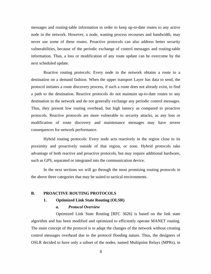
2. Classification of Routing Protocols Routing protocols for MANETs can be broadly classified into three main
categories:
Proactive routing protocols: Every node in the network has one or more routes to
any possible destination in its routing table at any given time. When data received from
the upper transport Layer is immediately transmitted to Layer 2, as at least one route to
the destination is already in the node’s routing table. Proactive protocols present low
latency, but medium to high routing overhead, as the nodes periodically exchange control
8
messages and routing-table information in order to keep up-to-date routes to any active
node in the network. However, a node, wasting process recourses and bandwidth, may
never use some of these routes. Proactive protocols can also address better security
vulnerabilities, because of the periodic exchange of control messages and routing-table
information. Thus, a loss or modification of any route update can be overcome by the
next scheduled update.
Reactive routing protocols: Every node in the network obtains a route to a
destination on a demand fashion. When the upper transport Layer has data to send, the
protocol initiates a route discovery process, if such a route does not already exist, to find
a path to the destination. Reactive protocols do not maintain up-to-date routes to any
destination in the network and do not generally exchange any periodic control messages.
Thus, they present low routing overhead, but high latency as compared to proactive
protocols. Reactive protocols are more vulnerable to security attacks, as any loss or
modification of route discovery and maintenance messages may have severe
consequences for network performance.
Hybrid routing protocols: Every node acts reactively in the region close to its
proximity and proactively outside of that region, or zone. Hybrid protocols take
advantage of both reactive and proactive protocols, but may require additional hardware,
such as GPS, separated or integrated into the communication device.
In the next sections we will go through the most promising routing protocols in
the above three categories that may be suited to tactical environments.
B. PROACTIVE ROUTING PROTOCOLS
1. Optimized Link State Routing (OLSR)
a. Protocol Overview Optimized Link State Routing [RFC 3626] is based on the link state
algorithm and has been modified and optimized to efficiently operate MANET routing.
The main concept of the protocol is to adapt the changes of the network without creating
control messages overhead due to the protocol flooding nature. Thus, the designers of
OSLR decided to have only a subset of the nodes, named Multipoint Relays (MPRs), in

9
the network responsible for broadcasting control messages and generating link state
information. A second optimization is that every MPR may choose to broadcast link state
information only between itself and the nodes that have selected it as an MPR.
Optimized Link State Routing is also designed to combine two separate
sets of functions. The core set of functions consists of all the protocol functions in play
when the protocol operates in a pure MANET, running OLSR as the Layer 3 protocol. A
second set of functions provides the additional necessary functions when a node has more
than one network’s devices and participates in more than one routing domain.
b. Multipoint Relay Nodes In OSLR, only multipoint relays (MPR) are designated for link state
updates and packet forwarding. In a typical flooding-based approach, a node broadcasts a
message either if it is the originator or if it has not received this message before. Thus,
the number of messages transmitted in the network is almost as large as the number of the
nodes in the network. Figure 1a shows a typical flooding scenario. Figure 1b shows the
flooding in the entire network when using MPRs.
Figure 1. Pure flooding and MPR flooding

10
As we can see in Figure 1b, only the MPRs, the grey-colored nodes,
broadcast messages in the network. It is clear that the number of broadcasted messages
can be greatly reduced by the MPRs’ implementation.
Although the optimal number of MPRs for a node reflects a smaller
number of broadcasting messages in the network, MPR selection is based only on a
heuristic that is proposed in [RFC 3626]. The set that consists of the nodes that are
multipoint Relays is called MPR set. Each node N in the network selects an MPR set that
processes and forwards every link state packet that node N originates. The neighboring
nodes of N that are not in the MPR set process this packet but do not further broadcast it.
A node N also maintains a subset of neighbors, named MPR selectors, which is the set of
the neighbors that have selected N as one of their MPRs. Each node may have one or
more MPRs. A condition for the selection of an MPR node is the assurance of
bidirectional links between it and its selectors.
c. Packet and Messages Format OLSR provides each node with one or more OLSR interfaces (an OLSR
interface is a network device participating in a MANET running OLSR). This is achieved
by the design and implementation of a unified packet format in which each packet
consists of one or more different types of messages. All the messages in a packet share a
common header, so nodes are able to retransmit messages of an unknown type. OSLR
uses User Datagram Protocol (UDP) as a transport-layer protocol for packet transmission
in Port 698. Figure 2 shows the packet format of OLSR.

11
Figure 2. OLSR Packet Format [RFC 3626]
Packet Length: is the length (in bytes) of the packet.
Packet Sequence Number: is incremented by one each time a new OLSR
packet is transmitted.
Message Type: indicates the type of message that is the "MESSAGE"
part.
Vtime: indicates the length of time after reception, that a node has to
consider valid the information obtained in the message.
Message Size: is the size of the message in bytes.
Originator Address: is the main address of the node that sent the
message. A node may have multiple interfaces with only one address for every interface.
However, each node must define a unique “main” address among the set of addresses that
the node has.

12
Time To Live: is the maximum number of hops a message will be
transmitted.
Hop Count: indicates the number of hops that the message has visited.
The originator sets this value to zero.
Message Sequence Number: is the unique identification number,
assigned to message by the source.
HELLO messages perform three independent tasks: link sensing (between
a node’s interface and neighboring interfaces), neighborhood discovery, and MPR
selection signaling. Link sensing and neighbor detection offer each node a list of
neighbors with which the node can directly communicate and afterwards the algorithm of
selecting MPRs is taking place. Basically, an MPR is selected in a way that ensures that
all the messages broadcast by a node that is a selector of this MPR will be received by all
nodes within a distance of 2 hops from the source node.
The HELLO message is encapsulated inside an OSLR packet and, in that
case, the Message-type field of the packet is set to HELLO_MESSAGE. Figure 3 shows
the format of a HELLO message.
Figure 3. OSLR HELLO Message Format [RFC 3626]

13
Reserved: all 0s.
Htime: is the time between two HELLO messages sent by a node.
Willingness: specifies the willingness of a node to carry and forward
traffic for other nodes. Possible values are WILL_NEVER, WILL_ALWAYS, MUST,
and WILL_DEFAULT.
Link Code: specifies information about the link between the interface of
the sender and a subsequent list of neighbor interfaces. It also specifies information about
the status of the neighbor.
Link Message Size: is the size of the link message, counted in bytes and
measured from the beginning of the "Link Code" field and until the next "Link Code"
field.
Neighbor Interface Address: is the address of an interface of a neighbor
node.
In OLSR, each node keeps network topology information in a table that is
used for routing-table calculations. This topological network information is disseminated
in the network with TC-type messages. A node must disseminate network topological
information between itself and the nodes in its MPR-selector set. Like all the previous
type of messages, TC messages are encapsulated in an OLSR packet, where the field
message type is set to TC_MESSAGE. Figure 4 shows the TC-message format.
Figure 4. OSLR TC Message Format [RFC 3626]

14
Advertised Neighbor Sequence Number (ANSN): The sequence number
for keeping up-to-date information about a node’s neighbor set.
Advertised Neighbor Main Address: The main address of a neighbor
node.
Reserved: Default value is set to 0000000000000000.
We saw above that a node running OLSR might have more than one
OLSR interface (network device). When a node has just one OLSR interface, the address
of the interface is the “main” address of the node. However, when a node has multiple
interfaces, it chooses one of those addresses to be the node’s “main” address. The
resolution between multiple interface addresses and the node’s main address is done by
exchanging Multiple Interface Declaration (MID) messages. Every node with multiple
interfaces periodically announces information describing its interface configuration to
other nodes in the network. MPRs are assigned to accomplish this task. Figure 5 shows
the format of an MID message.
Figure 5. OSLR MID Message Format [RFC 3626]
OLSR Interface Address: Contains the address of an OLSR interface of
a node, excluding the node’s main address (which is already indicated in the originator
address).
To provide interconnection with other routing domains when a MANET is
used to expand existing wired or wireless networks, a node uses a Host and Network
Association (HNA) message. The HNA_MESSAGE is encapsulated in the same way as
other types of messages, in an OLSR packet. Figure 6 shows the Host and Network
Association (HNA) message format.

15
Figure 6. OSLR HNA Message Format [RFC 3626]
Network Address: The network address of the associated network.
Netmask: The net mask, corresponds to the network address immediately
above it.
d. Route Discovery and Maintenance Each node in a network maintains a routing table that enables a source
node to send data packets to a destination node. Four different types of information are
used for the construction, calculation and maintenance of routing information. Every
node in the network obtains all the information necessary for the construction of its
routing table with a periodic transmission of messages. The node, upon receiving this
information, updates and recalculates its routing table. As we described above,
paragraphs MPRs are assigned this task. When a link breaks or if the network topology
changes due to a change in a node position in the network, no messages other than those
defined above are required for the update of the routing table. Figure 7 shows the
structure of a node’s routing table in OLSR.

16
Figure 7. OSLR Routing Table [RFC 3626]
e. Security OLSR does not provide security mechanism to ensure that nodes do not
intentionally provide false routing information. OLSR designers assume that there are
already additional security mechanisms in place at the lower layers of the network.
However, any persistent attack to any of the MPRs will result in flooding false link state
information to other nodes. We will see further in the next sections that most of the
proposed routing protocols for MANETs depend for their proper function on additional
security mechanisms that will be in place in the network.
f. Conclusions The main advantages of OLSR are low latency and high data delivery ratio
because each node in the network maintains an up-to-date routing table with all the
destinations in the network. Thus, no additional connection set-up time is required for a
node to send data packets to another node in the network. This proactive nature of OLSR
makes it a very attractive solution in networks where low latency and high data delivery
ratio are the main concerns. However, the main disadvantage of this protocol comes from
its proactive nature and the flooding mechanism, despite the use of the MPRs. OLSR may
introduce high routing overhead, consuming a large portion of the available bandwidth.
OLSR does not support multicasting routing.
2. Destination Sequenced Distance Vector (DSDV)
a. Protocol Overview Destination Sequenced Distance Vector [Perkins 1994] is a loop free
routing protocol in which the shortest-path calculation is based on the Bellman-Ford

17
algorithm. Data packets are transmitted between the nodes using routing tables stored at
each node. Each routing table contains all the possible destinations from a node to any
other node in the network and also the number of hops to each destination.
The protocol has three main attributes: to avoid loops, to resolve the
“count to infinity” problem, and to reduce high routing overhead. Each node issues a
sequence number that is attached to every new routing-table update message and uses
two different types of routing-table updates, named “full” and “incremental dumps”,
respectively, to minimize the number of control messages disseminated in the network.
Each node keeps statistical data concerning the average setting time of a message that the
node receives from any neighboring node. The data is used to reduce the number of
rebroadcasts of possible routing entries that may arrive at a node from different paths but
with the same sequence number. DSDV takes into account only bidirectional links
between nodes.
b. Route Discovery and Maintenance DSDV routing-table construction starts with the condition that every node
in the network periodically exchange control messages with its neighbors to set up multi-
hop paths to any other node in the network, in accordance with the Bellman-Form
algorithm. Each individual route to every destination is tagged with a destination
sequence number, which is issued by the destination node. Any route to a destination
with a higher destination sequence number replaces the same route with a smaller
destination sequence number in the node’s routing table, regardless of the number of hops
to this destination. Every node immediately advertises any significant change in its
routing table, such as a link failure to its neighboring node(s), but waits for a certain
amount of time to advertise other changes.
This time, has called the “settling time”, is calculated by
maintaining, for every destination, a running, weighted average of the most recent
updates of the routes. By implementing this advertising scheme, DSDV tries to minimize
the number of route updates transmitted by a node. Thus, when a node receives a route
update for a destination from one of its neighboring nodes, and a few seconds later, it
receives a second update from a different neighboring node for the same destination with
the same destination sequence number, but a lower number of hops, the node does not

18
immediately broadcast the change in its routing table. This is highly possible in a
MANET, in which the network topology changes very dynamically. If this kind of policy
were not in place, the node would have to advertise two route updates within a short
period, causing its neighboring nodes to broadcast new route updates to its neighboring
nodes. For this purpose, each node maintains a table with the destination address, the last
settling time and the average settling time of this address. The node uses the information
in this table to check the stability of the route to a destination. Figure 8 shows the
structure of a node’s routing table.
Figure 8. DSDV Routing Table
Destination: The destination node.
Next Hop: The next hop to this destination.
Number of Hops: The number of hops to this destination.
Sequence Number: The sequence number issued by the destination node.
Install Time: When this entry was made.
Stable Data: A pointer to the previous table.
As the position of a node in a network constantly changes over time, each
node needs to advertise to its neighboring nodes any change in its routing table. However,
this approach can lead to a high overhead of control messages in the network, leaving no
available bandwidth for user data. Thus, DSDV designers came up with the concept of
full and partial routing-table advertisement. Within this design, each node that encounters

19
a change in the path to any destination may choose to advertise only this particular
change instead of its complete routing table. This partial advertisement of a node’s
routing table is called an “incremental update.” If many changes occur in a
node’s routing table, the node may choose to advertise full routing-table entries, called a
“full update,” instead of many incremental updates.
c. Security DSDV does not provide security mechanism to address security
vulnerabilities observed in MANETs. [Wang 2003] suggested that DSDV is vulnerable to
any malicious node that disseminates false routing updates due to periodic exchange of
routing-update massages. Thus, an attack to replace the destination sequence number in a
route-update packet may have a severe impact on the performance of the network.
d. Conclusions DSDV has certain advantages that cannot be overlooked. First, the
simplicity of the protocol is very similar to the classic Distance Vector, with only small
modifications to avoid loops, with the use of destination sequence numbers. DSDV also
presents low latency, as every node always has a route to any destination in the network.
However, DSDV does not scale well in networks with high mobility, as the broken links
create a “storm” of route updates. This situation may severely degrade network
performance, in which the available bandwidth is limited. Another disadvantage of
DSDV is that it does not support a sleeping mode, as every node in the network must
periodically broadcast changes or full updates of its routing table. Those frequent and
periodic route updates in the network will also result in high-energy consumption.
Finally, DSDV does not support multicasting routing.
3. Cluster-Head Gateway Switch Routing Protocol (CGSR)
a. Protocol Overview The routing protocols we have studied so far use a flat network topology
in which all nodes are assigned the same tasks in terms of the route discovery and
maintenance process. OLSR differs from other proactive protocols by the introduction of
multiple point relays. However, every node in a network with flat hierarchy must
maintain, in the worst case, a route to every possible destination in the network. As more
20
nodes join the network, the size of the routing-tables increases, resulting in large numbers
of control messages in the network.
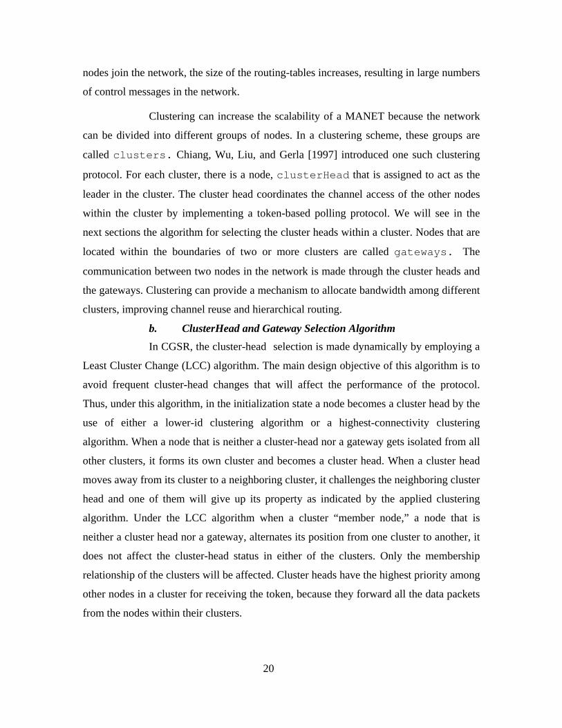
Clustering can increase the scalability of a MANET because the network
can be divided into different groups of nodes. In a clustering scheme, these groups are
called clusters. Chiang, Wu, Liu, and Gerla [1997] introduced one such clustering
protocol. For each cluster, there is a node, clusterHead that is assigned to act as the
leader in the cluster. The cluster head coordinates the channel access of the other nodes
within the cluster by implementing a token-based polling protocol. We will see in the
next sections the algorithm for selecting the cluster heads within a cluster. Nodes that are
located within the boundaries of two or more clusters are called gateways. The
communication between two nodes in the network is made through the cluster heads and
the gateways. Clustering can provide a mechanism to allocate bandwidth among different
clusters, improving channel reuse and hierarchical routing.
b. ClusterHead and Gateway Selection Algorithm In CGSR, the cluster-head selection is made dynamically by employing a
Least Cluster Change (LCC) algorithm. The main design objective of this algorithm is to
avoid frequent cluster-head changes that will affect the performance of the protocol.
Thus, under this algorithm, in the initialization state a node becomes a cluster head by the
use of either a lower-id clustering algorithm or a highest-connectivity clustering
algorithm. When a node that is neither a cluster-head nor a gateway gets isolated from all
other clusters, it forms its own cluster and becomes a cluster head. When a cluster head
moves away from its cluster to a neighboring cluster, it challenges the neighboring cluster
head and one of them will give up its property as indicated by the applied clustering
algorithm. Under the LCC algorithm when a cluster “member node,” a node that is
neither a cluster head nor a gateway, alternates its position from one cluster to another, it
does not affect the cluster-head status in either of the clusters. Only the membership
relationship of the clusters will be affected. Cluster heads have the highest priority among
other nodes in a cluster for receiving the token, because they forward all the data packets
from the nodes within their clusters.

21
A gateway, as it is located between two or more clusters, should be
able to communicate with all the cluster heads in whose clusters it exists as a member.
For this reason, a gateway is equipped with multiple radio interfaces to avoid conflicts
when the token is passed to the gateway, but it is tuned to another code. Therefore, every
node that participates in the network should be equipped with multiple radio interfaces,
since every node is expected to shift its status from a single node to either a cluster-head
or a gateway, and vice versa. Figure 9 shows the formation of clusters and the three
different kinds of nodes in a network.
Figure 9. CGSR Clusters Formation
c. Routing CGSR uses a combination of routing protocols. An extension of DSDV is
used for the construction of the routing tables, and the cluster routing protocol is used for
the channel accessibility within the cluster. Under DSDV, every node constructs two
tables with routing information. The first table contains node membership status, and the
second table, next-hop information. The node membership table matches every node in
22
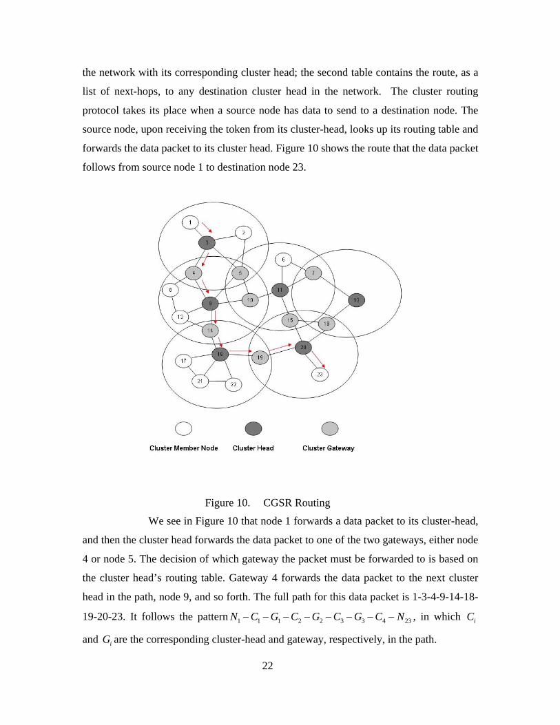
the network with its corresponding cluster head; the second table contains the route, as a
list of next-hops, to any destination cluster head in the network. The cluster routing
protocol takes its place when a source node has data to send to a destination node. The
source node, upon receiving the token from its cluster-head, looks up its routing table and
forwards the data packet to its cluster head. Figure 10 shows the route that the data packet
follows from source node 1 to destination node 23.
Figure 10. CGSR Routing
We see in Figure 10 that node 1 forwards a data packet to its cluster-head,
and then the cluster head forwards the data packet to one of the two gateways, either node
4 or node 5. The decision of which gateway the packet must be forwarded to is based on
the cluster head’s routing table. Gateway 4 forwards the data packet to the next cluster
head in the path, node 9, and so forth. The full path for this data packet is 1-3-4-9-14-18-
19-20-23. It follows the pattern 1 1 1 2 2 3 3 4 23N C G C G C G C N− − − − − − − − , in which iC
and iG are the corresponding cluster-head and gateway, respectively, in the path.

23
d. Security CGSR, like other routing protocols we have seen, does not provide any
security in the network. An attack can be directed toward a node, a gateway, or a cluster-
head. In the first case, the node will not be able to send or receive data, but this will affect
only the individual node, not network performance. In the second case, the cluster head
will be able to choose an alternate gateway to forward data packets. An attack toward the
cluster- head, however, will have severe consequences for network performance, because
the absence of the cluster-head in a cluster causes frequent employment of the LCC
algorithm.
e. Conclusions CGSR is a loop-free protocol, as the underlying protocol for populating
the routing-table entries is based on the DSDV, a loop free protocol. CGSR has certain
advantages over the other proactive protocols. First, it enables hierarchical routing, and
the path is recorded at the cluster level instead of at the single-node level, unlike DSDV
and OLSR. Second, this hierarchical scene can be used to implement a hierarchical
addresses scene. Hierarchical routing offers greater route robustness, resulting in a lower
dissemination of control messages for route repairs, and thus, more available bandwidth
for user data. Hierarchical addressing may offer more than one address for a single node
when the node is a member of two or more clusters. Therefore, at least one of these
addresses will be valid at any given time.
On the other hand, if a cluster-head has the same energy capabilities as its
cluster members, it will soon be out of order, as it will have to forward packets from
every node within its cluster.
CGSR clustering architecture provides a proper scheme for tactical
communications. In tactical scenarios, nodes in fact form a cluster e.g. a Platoon. The
Commander of the Platoon can play the role of the cluster-head, and his left, right, front,
and back limit then represent the gateways. Their communication devices can be
preconfigured and equipped with extra power sources and network interfaces to make
them able to perform these extra tasks. To avoid a single point of failure, two or three
nodes in the Platoon can be equipped with the same devices, to act as back-up for both
the cluster head and the gateways. This scene can also be expanded to create backbone

24
links between the Platoons in a Company and between Companies and the Battalion,
even when clusters do not necessarily overlap. Figure 11 shows a tactical implementation
of CGSR protocol. Nodes 5 and 21, 7 and 21, 15 and 10, are out of range and cannot set
up a link.
Figure 11. CGSR Tactical Implementation
4. Comparison of Proactive Routing Protocols Based on Qualitative
Metrics All the above proactive protocols are loop-free. OSLR, as a modification of the
link state algorithm, does not introduce any loops into the routing process, except for
oscillations when the link costs depend on the amount of traffic carried by the link. In the
MANET scheme, however, link cost depends on the number of hops from a source to a
destination, thus avoiding oscillations. DSDV solves the pathologies that the Distance
Vector algorithm introduces, by the use of destination sequence numbers. CGSR uses
DSDV as the underlying routing protocol, and thus it accordingly does not suffer from
any kind of loops in the network.
The proactive behavior of these protocols is guaranteed by the periodic exchange
of control messages. At any given time, every node has at least one route to any possible

25
destination in the network. We say “possible destination” because the physical existence
of a node in the network does not necessarily mean that the node is active or that a route
to the node exists, because the node may be out of the transmitting range of all other
nodes in the network.
None of the above protocols addresses the security vulnerabilities that are obvious
in wireless networks. The proper function of these protocols is based on an assumption
that all the nodes exist and operate in a secure environment where link-and physical-
Layer security mechanisms are in place. However, CGSR seems to be the most
vulnerable amongst DSDV and OLSR and, as explained in the previous sections, an
attack on nodes that act as cluster heads may have sever consequences for network
performance. DSDV is more secure than OLSR, as OLSR functionality is based on the
proper behavior of the MPRs.
DSDV and CGSR do not support unidirectional links. However, in wireless
communication, unidirectional links will exist and should be supported to take advantage
of any possible paths from a source node to a destination node. In MANETs, especially,
there is no such “luxury” as ignoring any possible paths, as routing protocols should take
advantage of any link to calculate routes in the network. OLSR designers take into
account these limitations of the wireless network and support both bidirectional and
unidirectional links.
As for the “sleep mode” operation, only OLSR considers some extensions in its
current existing design to support such an operation. In a wireless ad-hoc network, in
which nodes depend mainly on batteries for their energy source, the sleep mode is a
serious attribute that should be supported by any routing protocol.
Multicasting is not considered by any of the above protocols. In real situations in
tactical communications, data will be destined to a group of nodes, rather than to an
individual node. Unicasting will decrease the bandwidth available for user data when the
same message has to be delivered to multiple nodes.
We have also added three additional metrics, to point out the differences in the
design and implementation of the three protocols. We saw in the precious chapter why

26
the hierarchical routing philosophy of CGSR is better than the flat routing philosophy of
DSDV and OLSR.
The security and robustness of the protocol are also connected to the issue
whether or not the protocol functionality depends on nodes with “special” or “crucial”
tasks. Both OLSR and CGSR have nodes with special tasks.
The way that all the above protocols calculate their routes from a source node to a
destination node follows the shortest distance approach, which computes the smallest
number of hops between the source and the destination. However, as CGSR follows a
cluster head-to-gateway pattern for forwarding packets, it increases the number of hops
between a source and a destination node. Table 1 summarizes the performance of the
above protocols, based on qualitative metrics.
Table 1. Comparison of Proactive Protocols
By summarizing the above results, we can see that OLSR is closer to the IETF
MANET working-group design suggestions. Indeed, OLSR has been designed in high
respect to RFC 2501. Perhaps the only visible disadvantage is the high routing overhead.

27
However, it is mainly up to the network designer to decide what he really needs from a
network. In tactical communications, where the main concerns are timely and reliable
data delivery, OLSR may fit well as a routing protocol. If the concern is utilization of the
biggest portion of the available bandwidth, leaving a small portion for control messages,
then OLSR is not the best choice. On the other hand, the CGSR clustering scheme, as
shown in Figure 11, is very reflective of an army’s structure and communications and
could provide a good choice, with of course, a number of extensions and modifications.
Finally, given qualitative metrics and the attributes of the above protocols, we
choose OLSR for further evaluation in our simulation.
C. REACTIVE ROUTING PROTOCOLS
1. Ad Hoc On-Demand Distance Vector (AODV)
a. Protocol Overview Ad Hoc On-Demand Distance Vector, [RFC 3561] , is a reactive routing
protocol that is based on the Bellman-Form algorithm and uses originator and destination
sequence numbers to avoid both “loops” and the “count to infinity” problems that may
occur during the routing calculation process.
AODV, as a reactive routing protocol, does not explicitly maintain a route
for any possible destination in the network. However, its routing table maintains routing
information for any route that has been recently used within a time interval; so a node is
able to send data packets to any destination that exists in its routing table without
flooding the network with new Route Request (RREQ) messages. In this way, the
designers of AODV tried to minimize the routing overhead in the network caused by the
frequent generation of routing control messages.
A third characteristic of AODV is its ability to interconnect nodes in a
“pure” MANET running AODV with other non-AODV routing domains, thus extending
any network with fixed infrastructure to a network with both mobile wireless nodes and
static nodes, e.g., Ethernet.
A fourth characteristic of AODV is its support for both unicast and
multicast routing.

28
A final important characteristic of AODV is its ability to support both
bidirectional and unidirectional links, as in many cases in wireless communications, two
nodes in the network may only communicate with unidirectional links.
b. Messages Format AODV, unlike OLSR does not introduce any new packet formats, other
than control messages encapsulated in an IP datagram. AODV can operate with both IPv4
and IPv6 without any further modification.
Three types of messages are used for route-discovery and link-failure
notification: Route Request (RREQ) message, Route Reply (RREP) message, and Route
Error (RERR) message. When a sender node does not have a valid route to a destination
node in its routing table, it broadcasts a RREQ message. The destination node, or any
intermediate node with a valid route to the destination, replies to the RREQ message with
a RREP message. The RERR message is sent by a node to notify other affected nodes
when a link failure is detected. Figures 12, 13, and 14 show the formats of the above
three messages.
Figure 12. AODV Route Request Message Format [RFC 3561]
Type: 1
J, R, G, D, U: Flags
Reserved: All 0s

29
Hop Count: The number of hops from the originator of the request to the
node handling the request
RREQ ID: A unique identifier for the request
Destination IP Address: The address of the node to which the request has
been sent to acquire the route to the node
Destination Sequence Number: The last sequence number that is in the
originator’s routing table and was issued by the destination node
Originator IP Address: The IP address of the originator
Originator Sequence Number: The current sequence number issued by
the originator
Figure 13. AODV Route Reply Message Format [RFC 3561]
Type: 2
R, A: Flags
Reserved: All 0s
Prefix size: If nonzero, the 5-bit Prefix Size specifies that the
indicated next hop may be used for any node with the same routing prefix (as defined by
the Prefix Size) as the requested destination
Hop Count: The number of hops from the originator of the request to the
destination node
30
Destination IP Address: The address of the destination node
Destination Sequence Number: The destination sequence number related
to the route
Lifetime: The time in mills that the route is considered to be valid
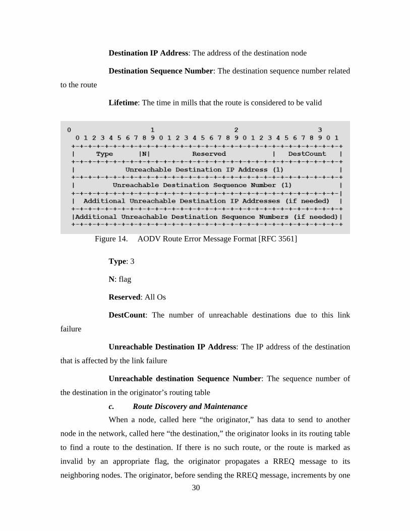
Figure 14. AODV Route Error Message Format [RFC 3561]
Type: 3
N: flag
Reserved: All Os
DestCount: The number of unreachable destinations due to this link
failure
Unreachable Destination IP Address: The IP address of the destination
that is affected by the link failure
Unreachable destination Sequence Number: The sequence number of
the destination in the originator’s routing table
c. Route Discovery and Maintenance When a node, called here “the originator,” has data to send to another
node in the network, called here “the destination,” the originator looks in its routing table
to find a route to the destination. If there is no such route, or the route is marked as
invalid by an appropriate flag, the originator propagates a RREQ message to its
neighboring nodes. The originator, before sending the RREQ message, increments by one

31
the RREQ ID and the originator sequence number in the message header. In this way,
each RREQ message is uniquely identified by combining the above numbers with the
originator IP address. Any intermediate node that receives an RREQ message, takes one
of the following three actions: First, the intermediate node discards the RREQ message if
it has previously received the same RREQ message. If the intermediate node has a valid
route to the destination node, it reverses a RREP message back to the originator. If the
intermediate node does not have a valid route to the destination, it further broadcasts the
message to its neighboring nodes. The destination node, which finally receives the RREQ
message, increments the destination sequence number and reverses an RREP message
back to the originator. When the originator node receives the RREP message, it updates
its routing table with the “fresh” route. Figure 15 shows the route discovery process from
source node 1 to destination node 10.
Figure 15. AODV Route Discovery Process
32
AODV uses mainly two mechanisms to avoid high routing overhead
caused by its flooding nature. The first mechanism involves a binary exponential back off
to minimize congestion in the network. The second one involves an expanding ring-
search technique in which the originator node starts broadcasting a RREQ message and
the TTL value is set to a minimum default value. If the originator node does not receive a
RREP message within a certain time interval, it exponentially increments the time
interval and increases the diameter of the searching ring. The maximum value for the ring
diameter is set by default to 35, which is, for AODV, the maximum value of the network
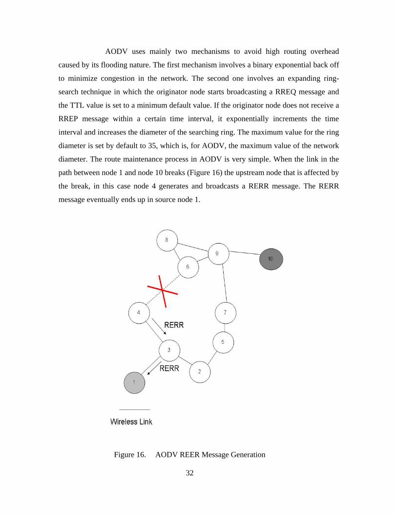
diameter. The route maintenance process in AODV is very simple. When the link in the
path between node 1 and node 10 breaks (Figure 16) the upstream node that is affected by
the break, in this case node 4 generates and broadcasts a RERR message. The RERR
message eventually ends up in source node 1.
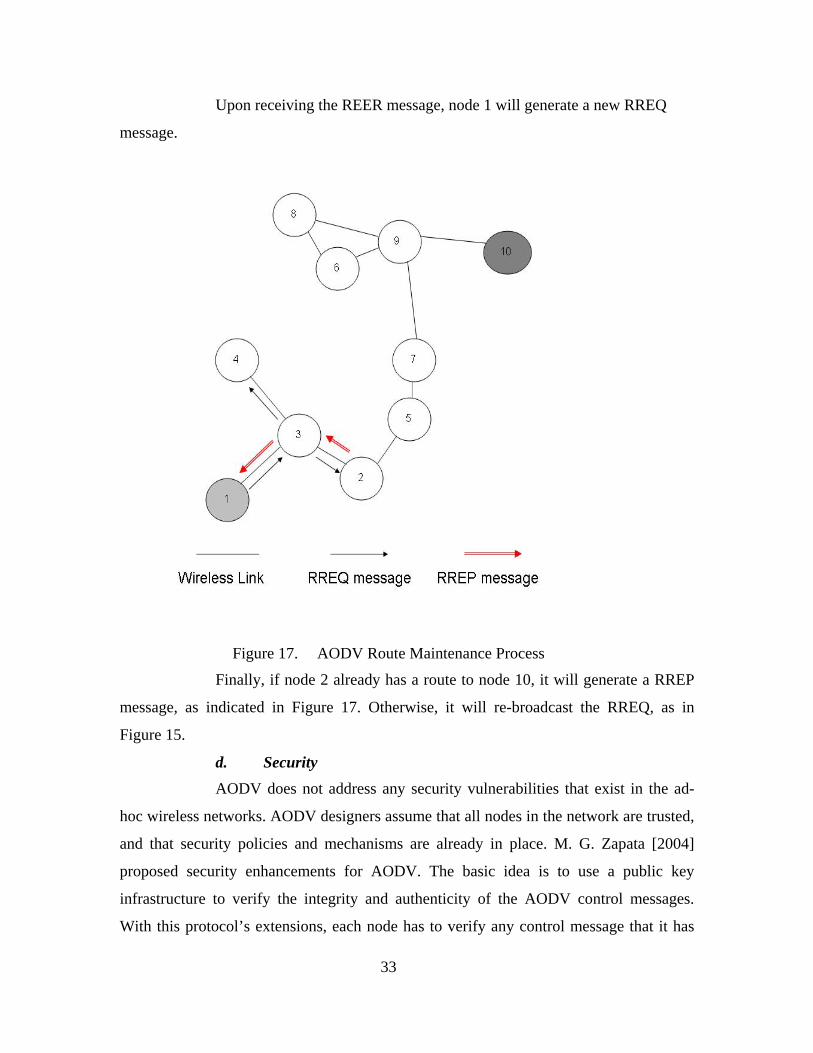
Figure 16. AODV REER Message Generation
33
Upon receiving the REER message, node 1 will generate a new RREQ
message.
Figure 17. AODV Route Maintenance Process
Finally, if node 2 already has a route to node 10, it will generate a RREP
message, as indicated in Figure 17. Otherwise, it will re-broadcast the RREQ, as in
Figure 15.
d. Security
AODV does not address any security vulnerabilities that exist in the ad-
hoc wireless networks. AODV designers assume that all nodes in the network are trusted,
and that security policies and mechanisms are already in place. M. G. Zapata [2004]
proposed security enhancements for AODV. The basic idea is to use a public key
infrastructure to verify the integrity and authenticity of the AODV control messages.
With this protocol’s extensions, each node has to verify any control message that it has

34
received from its neighboring nodes before further broadcasting the message. Although
the scope behind S-AODV is obvious, there are certain issues that we point out. First, the
use of public key infrastructure in such wireless networks is not as simple as it looks at
first sight. Second, the whole procedure will create further delay in the network, due to
greater processing time at the intermediate nodes. For tactical communications, the use of
symmetric keys at the lower Layers seems to be a more preferable solution.
e. Conclusions The two main advantages of AODV are its reactive nature, which reduces
the routing overhead in the network and the use of destination sequence numbers that
address routing loops and the “count to infinity” problem. However, control message
overhead can be introduced when every intermediate node originates a RREP message, to
satisfy a route discovery request if it has a valid route to the destination, causing a RREP
messages “storm”. Another disadvantage of AODV is that the propagation of periodic
HELLO messages from a node, to maintain connectivity with its neighboring nodes, will
lead to bandwidth consumption.
In conclusion, the simple design, the low routing overhead and the ring
searching technique make AODV an attractive solution for networks in which the
available bandwidth is limited and nodes can form organized groups. Security
weaknesses can be addressed by either modifying the protocol with the proposed security
extensions, or by applying security mechanisms at the lower layers.
2. Dynamic Source Routing Protocol (DSR)
a. Protocol Overview Dynamic Source Routing [Johnson, Maltz, and Broch 2004] is a simple
reactive protocol that is based on two main mechanisms: route discovery and route
maintenance. Both mechanisms are implemented in an ad-hoc fashion and in the absence
of any kind of periodic control messages. The main concept of the protocol is “source
routing”, in which nodes place in the header of a packet the route that the packet must
follow from a source to a destination. Each node “caches” the routes to any destination
it has recently used, or discovered by overhearing its neighbors’ transmission. When
there is not such route, a route discovery process is initiated. The protocol is designed for
a MANET of up to two hundreds nodes with high mobility rates and is loop-free. Other

35
important attributes of this protocol are its support for unidirectional links and
multicasting.
DSR can provide interconnection of wireless devices with multiple
network interfaces. This is an important attribute for tactical communications, as nodes in
the military need to have different signal ranges and thus different network devices.
b. Route Discovery When a node, “the originator,” wants to send a data packet to another node
in the network, “the destination,” it first looks in its Route Cache to find a route to
the destination. If such a route exists, the originator attaches to the packet header the
complete route to the destination and forwards the packet to the next node. The next node
checks the packet header and forwards the packet to the next node. The process
terminates when the packet reaches the destination.
If the originator cannot find a route to the destination in its Route Cache, it
initiates a route discovery process: it broadcasts a route request (RREQ) to its
neighboring nodes, adding a unique request ID to prevent other nodes from transmitting
the same request. Each of the neighboring nodes checks in its Route Cache, and if it finds
such a route, it sends a Route Reply (RREP) message back to the originator with the
complete path to the destination. Otherwise, the destination node is obliged to do this
task. DSR, by default, determines that a node may retransmit a RREQ message up to
sixteen times. However, to avoid a big number of control messages being disseminated in
the network, and sometimes for an inactive node, DSR uses expanding ring and
exponential back off mechanisms in the route discovery process. We have seen that
AODV also uses these two mechanisms for the same purpose.
In Figure 18, we assume that there is no path from source node 1 to
destination node 10, so node 1 initiates the routing discovery process. Node 9 discards the
RREQ message forwarded by node 7, as it has already received the same message from
node 6.

36
Figure 18. DSR RREQ Message Broadcasting
When node 10 receives the RREQ message, it initiates a RREP message
and attaches in the packet header the reverse path to node 1. Figure 19 shows the RREP
message process.

37
Figure 19. DSR RREP Message Processing
The wireless network device can contribute to the routing discovery
process by setting itself in a promiscuous mode, in which a node overhears transmission
from neighboring nodes. DSR takes advantage of this mode by caching for future use any
new route or multiple routes to the same destination. Thus, when a link breaks during
transmission, the originator may be able to find an alternate route to the destination
before sending a RREQ message. However, this design may lead to even greater latency
if, for instance, the originator tries multiple invalid paths before finally sending a new
RREQ message.
c. Route Maintenance Route maintenance in DSR is based on a distributed manner, by which
each node that originates or forwards a packet to the next node is responsible for
monitoring the validity of the link between the two nodes. This task can be achieved with
or without the exchange of acknowledgment messages between the two nodes. DSR may
use such an acknowledgment mechanism when it is already in place, as a standard of the
Layer 2 protocol (IEEE 802.11), or by overhearing the next node’s retransmission of the

38
packet, “passive acknowledgment,” provided there is a bidirectional link between the
transmitting and receiving node. If such mechanisms are not present, the transmitting
node can explicitly request an acknowledgment from the receiving node.
When the link between the two nodes breaks and the transmitting node
does not receive an acknowledgment from the receiving node, it retransmits the packet a
number of times, up to a threshold limit. When, after a certain number of retransmissions,
the node does not receive an acknowledgment, it first removes the route from its cache
and then originates a Route Error (RERR) message to inform all other nodes that use this
link to remove the route from their caches.
DSR has additional route maintenance features to improve its
functionality. A “packet salvaging” mechanism includes the actions taken by any
intermediate node when a link-break event is detected. Then the intermediate node, after
sending the Route Error (RERR) message, may search in its own route cache to find a
new route to the destination. When such a route exists, the intermediate node replaces the
original source route on the packet with the new route, marks the packet as “salvaged” to
prevent unnecessary retransmissions of the same packet by other nodes, and forwards the
packet to the new next node. An “automatic route shortening” mechanism starts when
any node in a route from a source to a destination detects that there is a shorter path than
the one indicated in the packet header from that node to the destination. In that case, the
node replaces the original source route with the new one and sends a Route Reply
(RREP) message back to the originator to update its route cache. The source node uses
“increased spreading of Route Error (RERR) messages” when it receives a Route Error
(REER) message. In that event, the originator piggybacks the RERR message on the new
RREQ, to prevent other nodes from generating RREP messages with the stale route that
caused the REER message.
d. Security Like many other routing protocols, DSR does not include a built-in
security mechanism to address MANET security vulnerabilities. The DSR designers
assume that all nodes that participate in the network are trusted and, if not, Layer 2 or
physical security mechanisms shall to be in place.

39
S. Buchegger and Le Boudec [2002] suggest security enhancements for
DSR, named CONFIDANT (Cooperation of Nodes, Fairness in Dynamic Ad-hoc
Networks), by which nodes monitor the behavior of their neighboring nodes and keep
statistical data to measure their neighbor’s contribution to the routing process. Based on
those metrics, nodes that detect the misbehavior of neighbors propagate an ALARM
message to inform other nodes in the network. Though conceptually correct, any such
built-in security functionality will increase the processing time and control messages
overhead in the network and although CPUs are getting more powerful today the
additional control messages with absorb a portion of the available bandwidth for user
traffic.
e. Conclusions The main advantage of DSR is the absence of any periodic control
messages that would take over a portion of the available bandwidth. The route discovery
and maintenance optimization techniques further eliminate the propagation and
dissemination of control messages. However, DSR does not employ any local repair of a
broken link and as any intermediate node can respond with a RREP message to a RERR
message, based on its route cache, there is a possibility for unstable routes in the network.
DSR was designed for a network with a limited number of nodes. High
mobility in the network will cause frequent link breaks that will result in high routing
overhead.
For tactical communications with low to medium mobility, DSR can be
one of the candidate protocols, as it does not require high-energy consumption because of
the lack of periodic updates. It can support multiple network interfaces, which are very
common in such communications, and it has low routing overhead, leaving useful
bandwidth for user traffic. The security vulnerabilities are the same as with all other
proposed routing protocols, and the solution is again symmetric or asymmetric key
infrastructure, or the security enhancements proposed in S. Buchegger and Le Boudec
[2002].

40
3. Temporally Ordered Routing Protocol
a. Protocol Overview All the routing protocols we have studied in the previous chapters are
based on link-state or distance-vector algorithms that find the shortest path, which is the
smallest number of hops between a source and a destination node in the network.
Temporally Ordered Routing Protocol, V.D. Park and M.S. Corson [2001], is a
distributed routing protocol that is based on the link reversal algorithm. The main concept
of this protocol is that the network for any source node can be “visualized” as a Directed
Acyclic Graph (DAG) rooted at the destination node. When a link between the source
and the destination fails, the nodes reverse the direction of the links and update the
previous nodes in the path. Additionally, each node maintains multiple paths to a given
destination and is capable of detecting any partitions in the network.
To accomplish such behavior, a value, “height,” is associated with each
node at all times. These values can be ordered in comparison to the “height” of each
neighboring node. Data flow occurs from a node with a higher value to a node with a
lower value. When a node cannot detect the height value of one of its neighbors, it does
not forward data packets to that node.
TORA disseminates control messages in a small local area, not in the
entire network, thus preserving bandwidth and minimizing processing time in the nodes.
When a link failure occurs, there is no need for a large-scaled dissemination of control
packets, as they can be limited to the small region where the link failure occurs.
TORA requires bidirectional links between the nodes in the network and
synchronization from an internal or external mechanism, e.g., Global Positioning System
(GPS). The protocol is loop-free, as the route formation is based on the DAG that is a
loop-free data structure, and supports only unicasting routing. TORA has four basic
functions: route discovery, route maintenance, route erasing, and route optimization.
Finally, TORA is not a self-operating protocol, but requires the existence
of the Internet MANET Encapsulation Protocol (IMEP) as the underlying network layer
protocol. [S. Corson, S. Papademetriou, P. Papadopoulos, V. Park, and A. Qayyum
1999].
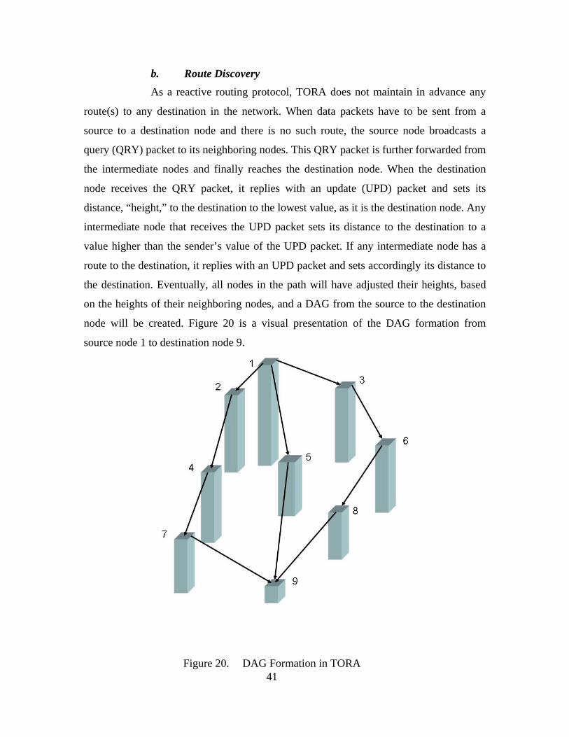
41
b. Route Discovery As a reactive routing protocol, TORA does not maintain in advance any
route(s) to any destination in the network. When data packets have to be sent from a
source to a destination node and there is no such route, the source node broadcasts a
query (QRY) packet to its neighboring nodes. This QRY packet is further forwarded from
the intermediate nodes and finally reaches the destination node. When the destination
node receives the QRY packet, it replies with an update (UPD) packet and sets its
distance, “height,” to the destination to the lowest value, as it is the destination node. Any
intermediate node that receives the UPD packet sets its distance to the destination to a
value higher than the sender’s value of the UPD packet. If any intermediate node has a
route to the destination, it replies with an UPD packet and sets accordingly its distance to
the destination. Eventually, all nodes in the path will have adjusted their heights, based
on the heights of their neighboring nodes, and a DAG from the source to the destination
node will be created. Figure 20 is a visual presentation of the DAG formation from
source node 1 to destination node 9.
Figure 20. DAG Formation in TORA
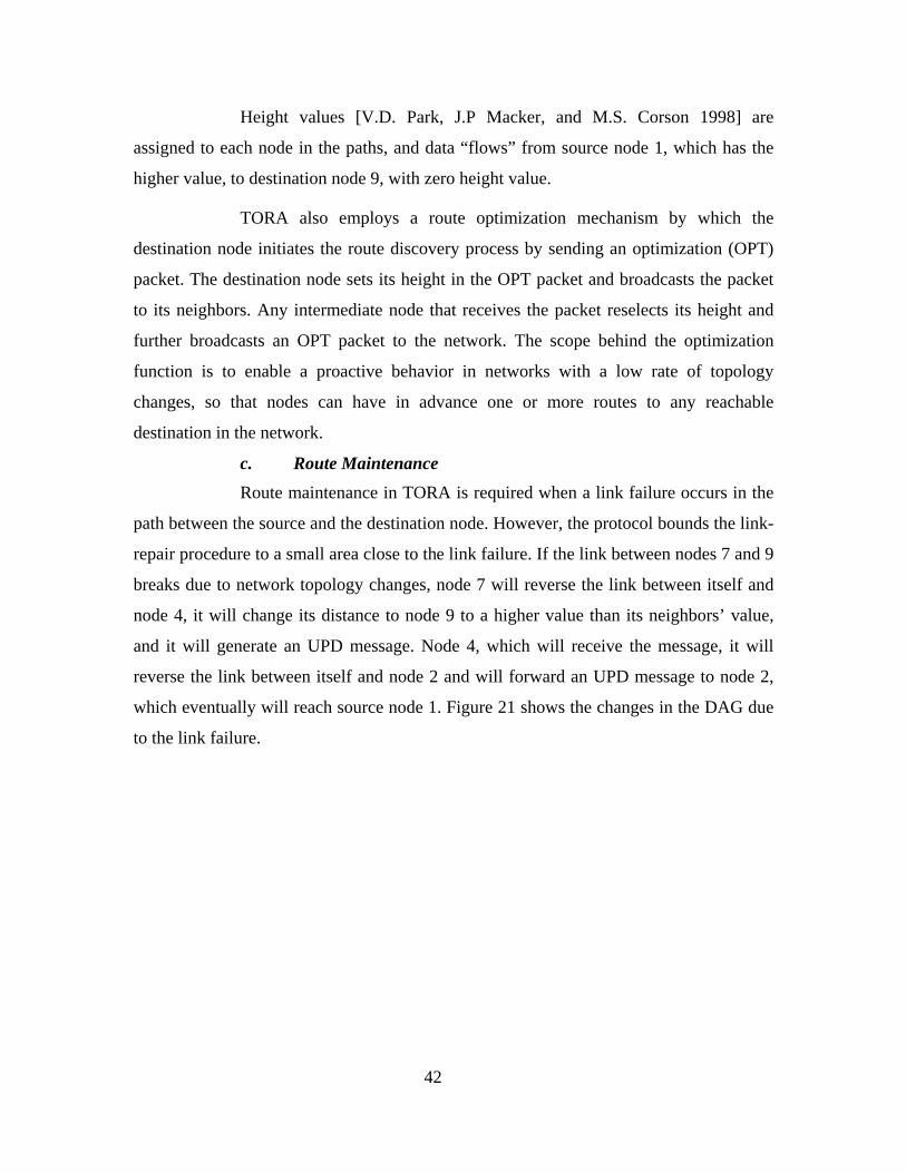
42
Height values [V.D. Park, J.P Macker, and M.S. Corson 1998] are
assigned to each node in the paths, and data “flows” from source node 1, which has the
higher value, to destination node 9, with zero height value.
TORA also employs a route optimization mechanism by which the
destination node initiates the route discovery process by sending an optimization (OPT)
packet. The destination node sets its height in the OPT packet and broadcasts the packet
to its neighbors. Any intermediate node that receives the packet reselects its height and
further broadcasts an OPT packet to the network. The scope behind the optimization
function is to enable a proactive behavior in networks with a low rate of topology
changes, so that nodes can have in advance one or more routes to any reachable
destination in the network.
c. Route Maintenance Route maintenance in TORA is required when a link failure occurs in the
path between the source and the destination node. However, the protocol bounds the link-
repair procedure to a small area close to the link failure. If the link between nodes 7 and 9
breaks due to network topology changes, node 7 will reverse the link between itself and
node 4, it will change its distance to node 9 to a higher value than its neighbors’ value,
and it will generate an UPD message. Node 4, which will receive the message, it will
reverse the link between itself and node 2 and will forward an UPD message to node 2,
which eventually will reach source node 1. Figure 21 shows the changes in the DAG due
to the link failure.

43
Figure 21. Link Break in TORA
In this example, node 1 has multiple alternate routes to destination node 9
that it will use to continue sending data packets. If node 1 did not have any alternate
routes, it would generate a QRY message, as was described in the previous section.
TORA also has the ability to detect any partition in the network. A
partition may occur when one or more nodes are unreachable from the source node. In
Figure 22, we can see how the protocol reacts when the link between nodes 4 and 2 fails.
Node 4 reverses the link between itself and node 2, and sends an UPD message to node 7.
However, the link reversal conflicts with the previous one in which the link between
nodes 7 and 9 failed. This is an indication of a network partition. When a node detects a
partition, it updates its link status table and broadcasts a clear (CLR) message to inform
other nodes of the network partition.

44
Figure 22. TORA Network Partition Detection
d. Security The protocol’s design does not take into account any MANET security
vulnerabilities. This is not surprising, as most ad-hoc routing protocols do not address
security problems and leave this issue to be solved by other security mechanisms that can
be applied in the network. However, protocol performance issues may arise if the
network experiences frequent and concurrent link failures. In that case, the broad
dissemination of UPD, and CLR messages in case of network partitions, will create
temporal oscillations.
[A. A. Pirzada, C. McDonald 2004] proposed a security encashment for
TORA, according to which, every node in the network can be set in promiscuous mode to
overhear transmissions of its neighboring nodes. Nodes under this mode can receive
additional information concerning the behavior of their neighbors and their contributions
to the routing and data packets dissemination process. Thus, nodes can detect any
malicious or malfunctioning nodes, based on a comparison between the original and the

45
retransmitted packets. A trusted table is used to stamp each node with a certain trust
level.
e. Conclusions The reactive nature of the protocol, along with its capacity to limit the
dissemination of control messages to the region close to a link failure, minimizes the
amount of routing control messages in the network. Multicasting and unidirectional-link
support are important attributes that TORA does not support. This is regarded as a
disadvantage of the protocol. However, TORA could be a good choice for large mobile
ad-hoc networks, in which link-state and distance-vector based algorithms will produce a
significantly large number of control messages due to frequent changes of the network
topology.
4. Comparison of Reactive Routing Protocols Based on Qualitative Metrics
All the above reactive protocols are loop-free. None addresses security
vulnerabilities that exist in a wireless ad-hoc network. However, there are certain
proposals for providing secure routing at Layer 3 for all the above protocols. Although
security is a major concern in military communications, we find that the proposed
security mechanisms will increase processing time, power consumption, and latency.
Note that reactive routing protocols already suffer from high latency in the network.
Only DSR in its current state, without any modification, can support both
bidirectional and unidirectional links. However, DSR will introduce high routing
overhead as routing information is stored at the data packets’ header. Thus, DSR will not
scale well in large networks if communicating nodes are located at opposite edges of the
network.
None of the three protocols supports the “sleep mode,” another important factor
for power preservation, especially in battery-powered mobile nodes. TORA seems to be a
more power-effective protocol, as it localizes most of its function in a small area, not in
the entire network. However, the exchange of HELO messages by the underlying IMEP
protocol will introduce power consumption. AODV will consume more power than DSR
due to the exchange of periodic HELO messages.

46
Only AODV supports multicasting, another important attribute of a routing
protocol. None of these protocols depends on any kind of node with special or crucial
tasks. All nodes in the network have the same tasks and play the same role in the routing
process. This is important, because the lack of “critical” nodes guarantees the inexistence
of any single point of failure in the network.
TORA does not necessarily find the shortest path between a source/destination
pair, as data flows form nodes with higher height to nodes with lower height. Table 2
summarizes the performance of the above protocols based on qualitative metrics.
Table 2. Comparison of Reactive Protocols
Finally, given qualitative metrics and the attributes of the three protocols, we
suggest that AODV and DSR would be good candidates for the routing protocol in
tactical mobile ad-hoc wireless networks. Therefore, we choose both AODV and DSR for
further evaluation in our simulation.

47
D. HYBRID ROUTING PROTOCOLS
1. Zone Routing Protocol (ZRP)
a. Protocol Overview Zone Routing Protocol [Haas, Z.J., Pearlman, M.R. and Samar, P. 2003] is
a distributed routing protocol that combines both a proactive and a reactive scheme for
route discovery and maintenance. The basic idea of the protocol is the creation of areas,
or zones, where every node proactively maintains one route or multiple routes to any
destination inside the zone and reactively obtains routing information for any node
outside of the zone. The zone diameter may be defined in advance, before nodes form the
network, or it may be optimized by every node, based on ZRP traffic measurements. The
radius of a node’s zone plays a significant role in the proper behavior of the protocol. If
the network consists of a large number of nodes with medium to low mobility or the
demand for routes is high, a large value for the radius is preferable to avoid the frequent
dissemination of routing requests and reply messages. On the other hand, if the network
consists of a small number of nodes with high mobility or the demand for routes is small,
the radius value should also be small to avoid overhead of periodic routing update
messages.
ZRP consists of two main protocols. The Intrazone Routing
Protocol (IARP) [Haas, Z.J., Pearlman, M.R. and Samar, P. 2003] is responsible for
finding and maintaining valid routes in the internal zones between any source/destination
pair at all times. Any proactive routing protocol that we studied in the previous sections,
such as DSDV, can be used as the ZRP IARP. The Interzone Routing
Protocol (IERP), [Haas, Z.J., Pearlman, M.R. and Samar, P. 2003] is responsible for
finding any available route outside of the node’s internal zone. The scope behind this
implementation is to reduce routing overhead and delay and to respond better in the
topological changes of the network.
Figure 23 shows the routing zones of node 10 with two different values for
the radius. In the first case, where 2radius = , node 10 maintains a small number of
available routes in its routing table. In the second case, where 3radius = , node 10

48
maintains more routes available in its routing table, in exchange for a larger number of
routing update messages. When 1radius = , ZRP behaves like a pure proactive protocol.
Figure 23. Routing Zones in ZRP
ZRP is a loop-free protocol and provides support for unidirectional links,
hierarchical routing, and interconnection with other non-ZRP routing domains when
every node’s network interface is assigned a unique IP address.
b. Route Discovery and Maintenance The route discovery process in ZRP depends on the location of the
destination node. If the destination node is located inside the source node’s intra zone, the
protocol acts like any other proactive protocol, thus ensuring that there is always a route
to any destination in the intra zone. When the destination node is located outside of the

49
source’s intra zone, the source node initiates a route discovery process and the IERP is
assigned to accomplish this task. To avoid large-scaled dissemination of routing request
messages ZRP employs a third protocol, the Bordercast Resolution Protocol
(BRP) [Haas, Z.J., Pearlman, M.R. and Samar, P. 2003], which is a sub-layer of the IERP
protocol. The BRP identifies the nodes that are located in the source node’s zone
perimeter and forwards the route request messages only to those peripheral nodes. Figure
24 shows the route discovery process from node 10 to node 8 for an intra zone,
2radius =
Figure 24. Route Discovery in ZRP
As node 8 is located outside the node 10 intra-zone, the BRP underlying
protocol border-casts the RREQ messages to the peripheral nodes 2, 3, 4, 6, 7, 13, 16, 18,
and 20. However, as nodes 3, 4, 9, and 14 already have a route to node 8, they initiate a
RREP message without further forwarding the RREQ message. When node 10 receives
multiple routes to the same destination, it stores the routes in its routing table and selects
50
the shortest one, based on the number of hops. We observe in the Figure 24 that there is a
possibility of collisions when multiple nodes transmit the RREP messages back to the
source. However, the border-casting scheme minimizes the propagation of RREQ
messages within a small region, except when the source/destination pair is located at
opposite edges of the network. When a peripheral node does not have a route to the
destination node, it originates a RREQ message and border-casts the message to its
peripheral nodes. That procedure continues until a route to the destination is found.
Route maintenance takes place when a node in an active route detects a
link failure in the route: the node employs a local reconfiguration of the path by searching
for an alternate route to the destination. If such a route exists, the node originates an
update message to inform all other nodes in the path and the source node of a change in
the path. The source node may continue sending data packets in the new non-optimized
route. If the source node wants to obtain a new optimal route, it regenerates a RREQ
message, as previously discussed.
c. Security ZRP does not employ any security mechanisms to ensure secure routing.
However, any security mechanisms that have been proposed for other routing protocols
can be applied to ZRP as well. Every node in the network can be in a promiscuous mode,
overhearing transmissions from its neighbors and gathering statistical data on its
neighbors’ behavior. Again, in this case, there is a trade-off between processing time,
latency, and security.
d. Conclusions ZRP seems to employ the best characteristics of both reactive and
proactive protocols. It avoids flooding the network with large-scaled Route Request
messages, as reactive protocols do, and the periodic exchange of HELLO messages in the
proactive scheme. Thus, ZRP reduces routing overhead in an inexpensive way. The only
visible drawback of the protocol is, perhaps, that its performance depends heavily on the
zone radius. For tactical communications, however, the zone radius can be set up in
advance, before the establishment of the network, as we know priory the data traffic, the
estimated velocity of the nodes, and the number of the nodes in the network. By

51
optimizing the zone radius, we can succeed in the high performance of the protocol, or at
least a better performance than any other “pure” proactive or reactive protocol.
2. Greedy Perimeter Stateless Routing (GPSR)
a. Protocol Overview Greedy Perimeter Stateless Routing [Carp and Kung 2000] is a hybrid
protocol whose functionality depends on knowledge of the geographic location of the
nodes in network. That knowledge can be obtained by integrating a GPS device into the
communication device or by other available means. Every node in the network must
know its own location and the location of its neighboring nodes. Thus, every node
periodically broadcasts its address and its location in x and y coordinates to all of its
neighboring nodes. Data-packet forwarding decisions are based on the locations of both
the source and the destination node. An address-to-location look-up algorithm is
implemented to map a node address to its location.
A periodic exchange of beacons, which encapsulate the node address and
location, is similar to the behavior of proactive protocols. The absence of any periodic
route table information is closer to the philosophy of reactive protocols.
GPSR employs two algorithms to forward data packets from a source to a
destination node: the greedy forwarding algorithm and the perimeter forwarding,
algorithm that will be explained in the section b. The objective of the protocol’s design is
to minimize routing overhead and increase the packet delivery ratio in a network, by
effectively responding to network topology changes without the dissemination of large-
scaled control messages.
Finally, GPSR makes use only of bidirectional links between a node and
its neighbors and does not support hierarchical routing.
b. Greedy and Perimeter Forwarding
In most cases, GPSR uses greedy forwarding for data packet delivery from
a source or any intermediate node to the next node. The greedy forwarding algorithm
needs to know the locations of a node’s neighbors and the location of the destination
node. According to this algorithm, the next-hop decision is based on the distance between
the next node and the destination node. Each node forwards data packets to the next node

52
that has the shortest distance to the destination node amongst other nodes in the node’s
“neighborhood”. We define a node’s “neighborhood” as the nodes within transmission
range of a node. Figure 25 shows greedy forwarding in GPSR. The curved doted lines
denote a node’s transmission range.
Figure 25. Greedy Forwarding in GPSR
However, greedy forwarding does not cover a case in which the distance
between an intermediate node and the destination is the lowest as compared to distances
from the intermediate node’s neighbors and the destination node. Figure 26 shows a case
in which the distance between node 4 and the destination node is the lowest compared to
the distances between node 5 and node 6 and the destination node. In this case, GPSR
employs “perimeter forwarding” in which node 4 stamps the data packet with a flag, to
indicate that the packet enters into perimeter forwarding, and forwards the data packet to
node 5 based on the “right hand rule”.

53
Figure 26. Perimeter Routing in GPSR
If a forwarding node (node 5 in Fig.26) has a neighbor (node 7 in Fig. 26)
with a shorter distance to the destination node, the forwarding node (5) removes the
“perimeter forwarding” flag, enters into “greedy forwarding”, and forwards the data
packet to the shorter-distance neighbor (7). The shorter-distance neighbor then uses
greedy forwarding to forward the data packet to the destination.
However, there is always a possibility in mobile wireless networks that a
destination node will be unreachable by any other node in the network. In that case, the
data packet travels around the perimeter trying to find a path to the destination. If a path
does not exist, the perimeter-forwarding algorithm never allows the packet to travel twice
across the same link in the same direction. If a node “sees” that the only possible way to
forward a data packet is to use a previous link toward the same direction, it drops the
packet. This function ensures the loop-free behavior of the protocol.

54
c. Security GPSR does not address any security vulnerabilities that exist in a mobile
wireless network. Any attack on the location-finding algorithm will have severe
consequences for the protocol’s performance because the proper behavior of the protocol
is built on its knowledge of the location of destination nodes.
d. Conclusions GPSR presents certain advantages over other protocols we have studied.
First, it does not use any type of control messages, such as route requests and error
messages. Second, it does not flood the network with any other type of control messages,
except those between a node and its neighbors, for location-finding purposes. Using
simulation results, B. Karp [2000] showed that GPSR outperforms even DSR, which is
known as a protocol with very low routing overhead in a network of up to 200 nodes’
compared to other routing protocols, in terms of packet delivery ratio and routing
overhead.
Perhaps the only visible drawback of GPSR is its dependence on
“external” devices, such as GPS, that increase the implementation cost. For tactical
implementation, this cost may be affordable; but we are not sure about commercial
implementation. The presence of a GPS device introduces another drawback if it does not
provide accurate node-location information. Any malfunction of the GPS device will
degrade the protocol’s performance and may lead to network crash.
3. Comparison of Hybrid Protocols Based on Qualitative Metrics Both ZRP and GPSR are loop-free protocols. ZRP ensures loop-free “behavior”
by employing loop-free protocols inside inter and intra-zones. On the other hand, GPSR’s
perimeter-forwarding algorithm never allows a packet to travel twice across the same link
toward the same direction.
ZRP’s proactive behavior is more obvious than that of GPSR, in which nodes
broadcast periodic beacons to their neighbors for location-update purposes. ZRP seems to
present higher routing overhead depending on the zone radius. ZRP behaves like any
other proactive protocol for the large value of this radius. However, one can optimize the
value of the zone radius to meet the needs of the wireless network. If low latency is the

55
main concern, reflecting lower data rates, the zone radius value should be high at least
a _ 1zone radius > .
None of the above protocols addresses the security vulnerabilities of wireless
networks. A possible solution is again monitoring the behavior of the nodes in the
network, or employing security mechanisms at the link or physical Layers. GPSR seems
to be more vulnerable than ZRP, as GPRS functionality is built on accurate location
advertisements by the nodes in the network. Any malfunction of the GPS devices will
degrade the protocol’s performance.
Only ZRP provides support for unidirectional links, hierarchical routing, and
interconnection with other non-ZRP routing domains. These are important attributes for a
routing protocol for MANETs as they provide the means for extending an existing
network with MANET technology, or interconnecting a MANET with other mobile and
fixed networks.
As for the “sleep mode” operation, none of these protocols directly supports such
an operation. The ZRP ‘‘sleep mode” depends on the routing protocols that operate in the
intra and inter zones. If OLSR is the routing protocol for the intra-zones, then ZRP can at
least partially support this mode.
GPSR does not support multicasting. Routing decisions are solely based on the
location of the destination node. On the other hand, ZRP depends on the “underlying”
routing protocols within the inter and intra-zones. If AODV is used as the routing
protocol for the inter-zones, it can provide multicasting support. Table 3 summarizes the
performance of the above protocols, based on qualitative metrics.

56
Table 3. Comparison of Hybrid Protocols
Given the above metrics and the attributes of the two protocols, we suggest that
ZRP would be a good candidate protocol in tactical mobile ad-hoc networks. Although
GPS devices may be supplied in the battlefield to each individual node, we do not wish to
base our communications structure on a variety of devices that increase the probability of
malfunctions and network failure. A promising attribute of ZRP is the optimization of the
zone radius to meet communication requirements. Hierarchical routing can reduce the
size of routing tables and offer better scalability in the network. However, the source
code [ZRP code] for ns-2 does not employ any optimization for protocol performance
making any comparison with other protocols meaningless.

57
III. SIMULATION
A. ROUTING PROTOCOLS CHOSEN FOR SIMULATION After the study and the evaluation of the routing protocols, based on qualitative
metrics in accordance with the RFC 2501, three routing protocols were chosen for
simulation and further evaluation in this thesis: OLSR, AODV and DSR.
B. SIMULATION SOFTWARE
1. The Network Simulator ns-2 The network simulator ns-2 [NS-2] is discrete event simulation software for
network simulations. Ns-2 began as a variant of the REAL network simulator [REAL
Network Simulator] in 1989. The latest version, ns-allinone-2.28, supports simulation for
four routing protocols for ad-hoc wireless networks such as AODV, TORA, DSDV, and
DSR. Ns-2 is written in C++ programming language and Object Tool Common Language
(OTCL). Although ns-2 can be built on various platforms, we chose a Linux platform
[FEDORA] for this thesis, as Linux offers a number of programming development tools
that can be used along with the simulation process.
To run a simulation with ns-2, the user must write the simulation script in OTCL,
get the simulation results in an output trace file, and analyze the results by using the awk
command, Perl scripts, or any other trace analysis available program. A sample
simulation script written in OTCL is shown in Appendix A. An output trace file is shown
in Appendix B. For this thesis, we developed our own program written in Java
programming language to analyze the ns-2 trace files and to calculate the four
quantitative metrics that we use for the evaluation of the tested routing protocols. Ns-2
also offers a visual representation of the simulated network by tracing nodes’ movements
and events and writing them in a network animator (NAM) file.
However, ns-2, an open software that has been built by a number of different
developers, suffers from a number of known and unknown bugs.
2. OLSR Routing Agent To install the OLSR protocol we obtained a copy of the source code from the
University of Murcia [UM-OLSR]. We recompiled and tested ns-2. The source code
complies with RFC 3626 but does not support the use of multiple interfaces as they are

58
defined in RFC 3626. OLSR multiple interfaces enable a mobile node to belong to
different routing domains. However, in our simulations, mobile nodes belong to the same
routing domain. OLSR code allows the user to define in the OTCL script the following
parameters for protocol performance optimization:
• Willingness: the willingness of a node to act as multipoint relay,
• A hello interval: the time interval between two HELLO messages, and
• A TC messages interval: the time interval between two TC messages.
By default, the values for node willingness, hello interval, and TC interval are 3,
2, and 5, respectively, in accordance with RFC 3626.
C. MOBILITY AND TRAFFIC SCENARIOS
1. Reference Point Group Mobility model (RPGM) Ns-2 requires node movements to either be defined in the OTCL script or to be
read from an external file. In this thesis, we used the Bonnmotion-1.3 software [Wall
2003], developed at the University of Bonn, to create mobile-node movement scenarios.
The RPGM [Hong 1999] is a mobility model in which mobile nodes move in clusters in
the simulation area. This model can create movements similar to military movements as
army troops move mainly by forming clusters. The movement of cluster-heads is
randomly chosen, and the movements of the cluster-members follow the direction of the
cluster-head. The type of parameters that can be used for the generation of the RPGM
mobility scenario is explained in Table 4.

59
Table 4. RPGM parameters in Bonnmotion-1.3
To generate a reference-point-group-mobile scenario, the user should write the
following command:
After the generation of scenario1, the user should type the following command to
transform scenario1 into a file that can be read by ns-2:
Figure 27 shows the creation of clusters as it is shown in the NAM console after
the end of the simulation.
./bm –f scenario1 RPGM –n 50 –d 100 –x 2000 –y 1000 –h 10.0 –l
3.0 –p 3.0 –a 3.0 –c 0.03 –r 170 –s 1.0
./bm NSFile –f scenario1

60
Figure 27. Creation of Clusters with the RPGM model 2. Manhattan Grid Mobility Model In this model, nodes move in predefined paths. By using Bonnmotion-1.3, we can
define the number of blocks along the x-axis and the y-axis, which will enable us to
define the size of blocks in a city. This is an important attribute of the model because it
enables us to create a scenario applicable to a specific targeted city in which mobile
nodes move. The type of parameters that can be used for the generation of the Manhattan
Grid mobility model is explained in Table 5.

61
Table 5. Manhattan Grid Model parameters in Bonnmotion-1.3
Figure 28 shows a screenshot of the NAM console at the end of the simulation
with that mobility model. What is important in that model is that nodes at opposite sides
of a block cannot communicate due to the reception failure posed by the blocks. As we
increase the size of blocks in the simulation area, the probability of data packet loss by
the mobile nodes increases.

62
Figure 28. Manhattan Grid Mobility Model
3. Traffic Scenarios NS-2 supports two different types of traffic for wireless ad-hoc networks. The
user can choose either the Transmission Control protocol (TCP) or Constant Bit Rate
(CBR). The traffic generator is located under the directory indep-utils/cmu-scen-gen and
the two tcl scripts tcpgen.tcl and cbrgen.tcl, can be used for traffic generation. In this
thesis, we used CBR as our traffic pattern. To create CBR connections the user should
run
where: -type, is cbr or tcp,
-nn, is the number of mobile nodes,
ns cbrgen.tcl –type cbr –nn 50 –seed 1.0 –mc 20 –rate 10.0 > cbr-outfile

63
-seed, is a random seed,
-mc, is the maximum number of connections,
-rate, is the number of packets per second.
The start times for the CBR connections are randomly chosen with a
maximum time value set to 180 sec. The user can change the start times in the cbr-outfile
to keep them within the limits of the simulation time. A sample cbr-outfile is shown in
Appendix C.
D. QUANTITATIVE METRICS
1. Introduction
RFC 2501 describes a number of quantitative metrics that can be used for
evaluating the performance of a routing protocol for mobile wireless ad-hoc networks. In
this thesis, we follow the general ideas described in RFC 2501, and we use four
quantitative metrics similar to those that were used in [Das, S.R., Perkins, C.E. Royer,
E.M. 2000]. The packet delivery ratio and average end-to-end delay are most important
for best-effort traffic. The normalized routing load will be used to evaluate the efficiency
of the routing protocol. Finally, the normalized MAC load is a measure of the effective
utilization of the wireless medium for data traffic. In the next sections, we will define
those four quantitative metrics.
2. Packet Delivery Ratio The packet delivery ratio is defined as the fraction of all the received data packets
at the destinations over the number of data packets sent by the sources. This is an
important metric in networks. If the application uses TCP as the layer 2 protocol, high
packet loss at the intermediate nodes will result in retransmissions by the sources that will
result in network congestion.
_ _ __ __ _ _
Total Data packets receivedPacket Delivery RatioTotal Data packets sent
=
3. Average End-to-End Delay End-to-end delay includes all possible delays in the network caused by route
discovery latency, retransmission by the intermediate nodes, processing delay, queuing
delay, and propagation delay. To average the end-to-end delay we add every delay for

64
each successful data packet delivery and divide that sum by the number of successfully
received data packets. This metric is important in delay sensitive applications such as
video and voice transmission.
( )_ __ 2 _
_ _ _Time received Time sent
Average End End DelayTotal Data packets receivedΣ −
=
4. Normalized Routing Load The normalized routing load is defined as the fraction of all routing control
packets sent by all nodes over the number of received data packets at the destination
nodes. This metric discloses how efficient the routing protocol is. Proactive protocols are
expected to have a higher normalized routing load than reactive ones. The bigger this
fraction is the less efficient the protocol.
_ _ __ __ _ _ e
Total Routing packets sentNormalized Routing LoadTotal Data packets r ceived
=
5. Normalized MAC Load The normalized MAC load is defined as the fraction of all control packets
(routing control packets, Clear-To-Send (CTS), Request-To-Send (RTS), Address
Resolution Protocol (ARP) requests and replies, and MAC ACKs) over the total number
of successfully received data packets. This is the metric for evaluating the effective
utilization of the wireless medium for data traffic.
_ _ __ __ _ _
Total Control packets sentNormalized MAC LoadTotal Data packets received
=
E. TRACE ANALYSIS SOFTWARE This program analyzes the ns-2 trace files and calculates the values of the above
four quantitative metrics. In the next section, we explain how to get those values from the
ns-2 trace file.
Calculating Packet Delivery Ratio
In ns-2 trace files a data packet is delivered at the destination node only if there is
a receive event with the same packet sequence number associated with the agent type
AGT. We build two lists, one of received and one of sent CBR packets with the agent

65
type AGT. For the sentPktList, we store values for transmission time and packet sequence
number. In the same way, we store the receiving time and the sequence packet number in
the rcvPktList. Two counters, named rcvPkts and sentPkt, are used to calculate the packet
delivery ratio.
Calculating Average End-to-end delay
For every packet in the sentPktList, we search its sequence number in the
rcvPktLis and store the transmission time. For each successful matching, we extract the
receiving time of that packet and calculate the end-to-end delay. To find the average end-
to-end delay we sum all the delays and divide by the number of rcvPkts.
Calculating Normalized Routing Load
We count all send events with agent type RTR and packet type any control packet
that the routing protocol generates. To calculate the normalized routing load we divide
the sum of all control routing packets by the number of rcvPkts.
Calculating Normalized MAC Load
We count all the send events with agent type MAC and packet type RTS, CTS,
ARP, and ACK and add to this number the sum of all control routing packets found in the
previous calculation. To calculate the normalized MAC load, we divide the sum of all
control packets (MAC and routing control packets) by the number of rcvPkts.
The program is able to provide the wished results for any size of trace file in a
few minutes and can be easily extended to include any routing protocol. The source code
of the Trace Analysis program is shown in Appendix D.

66
THIS PAGE INTENTIONALLY LEFT BLANK
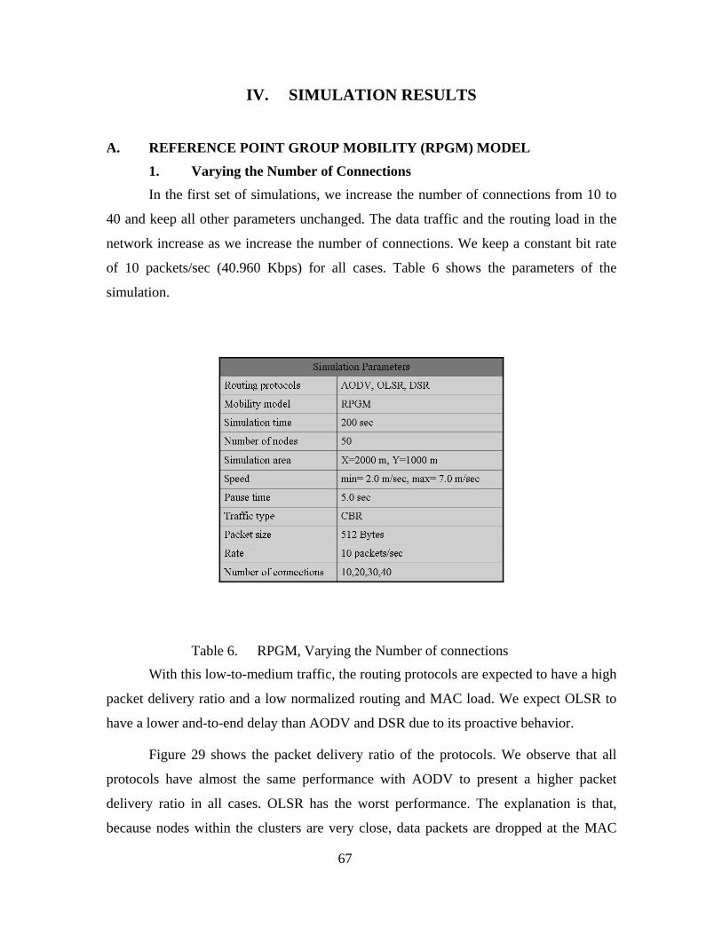
67
IV. SIMULATION RESULTS
A. REFERENCE POINT GROUP MOBILITY (RPGM) MODEL
1. Varying the Number of Connections In the first set of simulations, we increase the number of connections from 10 to
40 and keep all other parameters unchanged. The data traffic and the routing load in the
network increase as we increase the number of connections. We keep a constant bit rate
of 10 packets/sec (40.960 Kbps) for all cases. Table 6 shows the parameters of the
simulation.
Table 6. RPGM, Varying the Number of connections
With this low-to-medium traffic, the routing protocols are expected to have a high
packet delivery ratio and a low normalized routing and MAC load. We expect OLSR to
have a lower and-to-end delay than AODV and DSR due to its proactive behavior.
Figure 29 shows the packet delivery ratio of the protocols. We observe that all
protocols have almost the same performance with AODV to present a higher packet
delivery ratio in all cases. OLSR has the worst performance. The explanation is that,
because nodes within the clusters are very close, data packets are dropped at the MAC

68
layer. The reason being for that is that the network is congested at some point by the
periodic transmission of HELLO messages and OLSR routing packets. Therefore, the
existence of valid routes between a source/destination pair in a node’s routing table, does
not necessarily guarantee a better packet delivery ratio.
Increasing Number of Connections
0
20
40
60
80
100
120
10 20 30 40
Number of connections
Pack
et d
eliv
ery
ratio
(%)
AODVOLSRDSR
Figure 29. RPGM, Packet Delivery Ratio (Increasing number of connections)
Figure 30 shows the normalized routing load of the protocols. We observe that
OLSR has a normalized routing load 800 percent higher than AODV and DSR for 10
connections. With a higher number of connections, OLSR “stabilizes” its routing
overhead. This happens because, with a higher number of connections, the number of the
received packets at the destinations is getting higher while the number of OLSR routing
packets remains the same. As a result, the value of the normalized routing load fraction is
getting higher. AODV presents a higher routing load than DSR for an increased number
of connections, as nodes need to transmit a bigger number of routing control messages to
establish and maintain those additional connections. DSR seems to be the most stable
protocol regardless of the number of connections in the network due to its cashing
mechanism at the source and intermediate nodes.

69
Increasing Number of Connections
0
0.2
0.4
0.6
0.8
1
1.2
10 20 30 40
Number of connections
Nor
mal
ized
rout
ing
load
AODVOLSRDSR
Figure 30. RPGM, Normalized Routing Load (Increasing number of connections)
Figure 31 shows the normalized MAC load of the protocols. We observe that
OLSR has a higher MAC load than AODV and DSR for 10 and 20 connections.
However, with 30 and 40 connections, OLSR presents the lowest MAC load.
Increasing Number of Connections
00.5
11.5
22.5
33.5
44.5
5
10 20 30 40
Number of connections
Nor
mal
ized
MA
Clo
ad
AODVOLSRDSR
Figure 31. RPGM, Normalized MAC Load (Increasing number of connections)
The explanation is that both AODV and DSR generate a higher number of
messages at the MAC layer because more control messages are needed to satisfy the
establishment and maintenance of those new connections. The MAC layer generates

70
RTS, CTS, and ACK messages for each transmission of RREQ, RREP, and RERR
messages. Thus the higher the number of routing control messages, the higher the
normalized MAC load. On the other hand, OLSR generates those additional RTS, CTS,
and ACK messages at the MAC layer only for data packets transmission, as the time
interval for HELLO and other types of OLSR routing control packets remains unchanged,
regardless of the increased number of connections. The conclusion is that, although
AODV and DSR generate a lower number of routing control messages, the utilization of
the wireless medium by data traffic is better in OLSR in a network in which the number
of connections increases over time.
Finally, Figure 32 shows the average end-to-end delay of the protocols. OLSR has
the lowest and-to-end delay, which increases almost linearly with the number of
connections. DSR has lower end-to-end delay than AODV, although AODV employs a
similar chasing mechanism to that of DSR. This is because the timeout value for erasing
routes that has been used previously in AODV is not optimized to cover all possible
mobility and traffic scenarios. We observe that DSR has higher end-to-end delays for 30
connections for the same reason.
Increasing number of Connections
0
200
400
600
800
1000
1200
1400
10 20 30 40
Number of connections
Ave
rage
End
2End
del
ay(m
ilis)
AODVOLSRDSR
Figure 32. RPGM, End2End Delay (Increasing number of connections)

71
2. Varying the Network Load
In the second set of simulations, we increase the number of data packets sent by
the sources from 5 packets/sec (20.480 Kbps) to 20 packets/sec, (81.920 Kbps), keeping
all other network parameters unchanged. The demand for efficient routing and wireless
medium utilization for data traffic is higher in that scenario; we will observe how the
three protocols can scale in that demanding network. We observed that, under that
mobility scenario and a packet rate of more than 25 packets/sec (102.400 Kbps), all
protocols present a very low packet delivery ratio (below 50 percent), making any
comparison at those rates meaningless. Table 7 shows the parameters of the simulation.
Table 7. RPGM, Varying the Network load
Figure 33 shows the packet delivery ratio of the protocols. All protocols have an
identical performance at low rates (5 packets/sec). DSR outperforms AODV and OLSR
in all cases, whereas OLSR has, again, the worst performance. Although we placed 50
nodes in an area of 2000 x 1000 meters to avoid interference, nodes are still in close
proximity, especially within the clusters. This scenario does not favor OLSR: we noticed
by analyzing the ns-2 trace files that OLSR produces a fairly large size of route update
packets that require higher transmission time than that of AODV and DSR. Neither

72
AODV nor DSR suffers from that periodic exchange of link state information, as routes
are discovered in an ad-hoc fashion. By analyzing also the trace files, we observed that
data packets are dropped by AODV for the following reason.
a) In AODV, the source node will send a RREQ message if a route to the
destination node does not exist. After the second transmission of the RREQ message, if
the source node does not receive a RREP message within a time interval, it will drop the
first packet in the queue and repeat the same procedure for the second data packet in the
queue. However, if any intermediate node cannot find a valid route to the destination
node by repeating the above procedure, it will drop not only the first packet but also all
data packets from its queue, thereby degrading the protocol’s performance.
Increasing Number of Packets
0
20
40
60
80
100
120
5 10 15 20
Packets/sec
Pack
et d
eliv
ery
ratio
(%)
AODVOLSRDSR
Figure 33. RPGM, Packet Delivery Ratio (Increasing number of packets)
Figure 34 shows the normalized routing load. DSR has the lowest routing load at
all packet rates, showing that it scales well in networks with low mobility in which data
traffic increases over time. OLSR has a high routing load in low traffic (5packets/sec),
which drops significantly in higher traffic. AODV has a higher routing load than DSR,
although, like DSR, it employs an expanding ring and cashing mechanism. However,
AODV was designed for networks with a larger number of nodes and higher mobility
than that in our simulation.

73
Increasing Number of Packets
00.10.20.30.40.50.60.70.80.9
5 10 15 20
Packets/sec
Nor
mal
ized
rout
ing
load
AODVOLSRDSR
Figure 34. RPGM, Normalized Routing Load (Increasing number of packets)
Figure 35 shows the normalized MAC load. DSR has the best performance at all
rates. We observe also that AODV has a higher MAC load than OLSR, although the
AODV routing load is lower than that in OLSR. We explained in the previous section
why that happens.
Figure 36 shows the end-to-end delay. We expected OSLR to have better
performance than the other two reactive protocols. However, the end-to-end delay in
OLSR increases when the data traffic increases. The explanation lies in the low mobility
of the network. As nodes do not change their positions very frequently, there exists a high
level of network congestion at certain regions of the network because none of the three
protocols employs any mechanism for load balancing, data traffic is not evenly
distributed in the network, and high end-to-end delays result.

74
Increasing Number of Packets
0
1
2
3
4
5
6
5 10 15 20
Packets/sec
Nor
mal
ized
MA
C lo
adAODVOLSRDSR
Figure 35. RPGM, Normalized MAC Load (Increasing number of packets)
Increasing Number of Packets
0500
100015002000250030003500400045005000
5 10 15 20
Packets/sec
Ave
rage
End
2End
del
ay(m
illis
) AODVOLSRDSR
Figure 36. RPGM, End2End Delay (Increasing number of packets)
3. Distributing the Network Load In the third set of simulations, we distribute the network load so that 66 percent of
the data packets are destined within the clusters and 33 percent are destined to a cluster at
a central position in the simulation area. We do that to approximate a real situation
scenario in which a node within each cluster, which we arbitrarily choose to be the cluster

75
head, communicates with its neighboring nodes within the cluster and with other nodes at
a central position in the simulation area, which represents the Headquarters (HQ) of the
unit. As none of the protocols employs a mechanism for balancing the network load, we
expect all the protocols to have a lower performance than in our previous scenario. This
is because nodes around the central cluster behave as “bottlenecks” of the network,
dropping data packets. However, this is a real situation in tactical communications, and
we wish to analyze the behavior of the tested protocols under that scenario. Table 8
shows the parameters of the simulation.
Table 8. RPGM, Distributing the Network load
Figure 37 shows the packet delivery ratio. All protocols present almost identical
performance, which is lower than in our previous scenario. That at least indicates that all
three protocols can be used for any traffic scenario in a network with a low number of
nodes, medium data traffic, and medium mobility.

76
Distributed Network Load
0
20
40
60
80
100
120
5 10 15 20
Packets/sec
Pack
et d
eliv
ery
ratio
(%)
AODVOLSRDSR
Figure 37. RPGM, Packet Delivery Ratio (Distributing the Network load)
Figure 38 shows the normalized routing load of the protocols. We observe that
DSR has the lowest routing load that remains stable regardless of the data packet rate.
AODV, in contrast, presents the highest routing load. We explained in the previous
section that the reason for AODV’s high routing load lies in the design of AODV, which
performs better in larger networks with a higher mobility.
Distributed Network Load
00.10.20.30.40.50.60.70.80.9
5 10 15 20
Packets/sec
Nor
mal
ized
rout
ing
load
AODVOLSRDSR
Figure 38. RPGM, Normalized Routing Load (Distributing the Network load)

77
Figure 39 shows the normalized MAC load. OLSR again presents the lowest
MAC load, while the DSR performance is the most stable. AODV has the highest MAC
load at lower data packet rates; that drops when the data packet rates increase.
Distributed Network Load
4.4
4.6
4.8
5
5.2
5.4
5.6
5.8
6
5 10 15 20
Packets/sec
Nor
mal
ized
MA
C lo
ad
AODVOLSRDSR
Figure 39. RPGM, Normalized MAC Load (Distributing the Network load)
Finally, figure 40 shows the average end-to-end delay of the protocols. OLSR has
the lowest end-to-end delay at lower rates while DSR has the lowest end-to-end delay at
higher rates.
Distributed Network Load
0
500
1000
1500
2000
2500
5 10 15 20
Packets/sec
Ave
rage
End
2End
del
ay(m
illis
) AODVOLSRDSR
Figure 40. RPGM, End2End Delay (Distributing the Network load)

78
What is interesting in the above results is that OLSR presents the highest end-to-
end delay at higher data packet rates. By analyzing the simulation trace files, we observed
that the size of OLSR TC messages is within the range (48, 2020) bytes. Every 5 seconds
all MPR nodes flood the network with TC messages. In our ns-2 implementation, we
configured the node’s interface queue in such a way that all routing control messages
have the highest priority amongst other types of packets, so routing protocols can adapt
the network changes in a timely manner. However, that size of TC messages in OLSR
causes high end-to-end delay for data packets due to processing, transmission, and
propagation delays at the intermediate nodes. In conclusion, the proactive attribute of a
protocol does not necessarily guarantee a lower end-to-end delay. Routing control
packets size, mobility, and data traffic all affect protocol performance, and, under
scenarios, like in the one above, a proactive routing protocol may introduce higher end-
to-end delay than a reactive routing protocol.
4. Varying Network Mobility In the fourth set of simulations, we vary nodes’ mobility. We start with a mobility
scenario in which the nodes have a low velocity of 5 m/sec (18 Km/h). We then increase
nodes’ velocity up to 20 m/sec (72 Km/h). Our intention is to investigate the behavior of
the three protocols in networks with varied mobility, although the high mobility, 72
Km/h, cannot be easily found in tactical movements.
We keep a constant data rate of 10 packets/sec (40.960 Kbps) and a constant
number of 20 connections. We observed that, at higher data rates with increasing
mobility, the performance of the protocols decreases due to network congestion in a way
that makes any comparison meaningless. Table 9 shows the simulation parameters.

79
Table 9. RPGM, Varying Network Mobility
Figure 41 shows the packet delivery ratio of the protocols. All protocols, present a
similar performance with AODV, having the best performance at all mobility rates. We
observe again that protocols have a better performance when the speed of the nodes is 10
m/sec and 15 m/sec, because the network load is more evenly distributed among the
nodes at higher mobility rates.
Figure 42 shows the normalized routing load. DSR has the best performance with
an increase of the routing load at a higher mobility. That stable behavior of DSR is a
desirable property of a protocol as it indicates that it can scale well in networks in which
the mobility changes over time. OLSR has the same behavior, while the AODV
performance increases when nodes move at higher speeds.

80
Increasing Network Mobility
0102030405060708090
100
5 10 15 20
Velocity in m/sec
Pack
et d
eliv
ery
ratio
(%)
AODVOLSRDSR
Figure 41. RPGM, Packet Delivery Ratio (Varying Network Mobility)
Increasing Network Mobility
00.10.20.30.40.50.60.70.80.9
5 10 15 20
Velocity in m/sec
Nor
mal
ized
rout
ing
load
AODVOLSRDSR
Figure 42. RPGM, Normalized Routing Load (Varying Network Mobility)
Figure 43 shows the normalized routing load. AODV has lower normalized MAC
load than DSR, despite having a higher normalized routing load. The explanation is that
under this simulation scenario, the route discovery in AODV is more accurate than in
DSR. DSR, as a result, generates a higher number of routing control messages than

81
AODV to discover alternate routes at the intermediate nodes. OLSR is the most stable
protocol in terms of the normalized MAC load in networks with varying mobility.
Increasing Network Mobility
0
2
4
6
8
10
12
5 10 15 20
Velocity in m/sec
Nor
mal
ized
MA
Clo
ad
AODVOLSRDSR
Figure 43. RPGM, Normalized MAC Load (Varying Network Mobility)
Figure 44 shows the end-to-end delay of the protocols. OLSR has the lowest end-
to-end delay at low and high mobility, while AODV outperforms DSR.
Increasing Network Mobility
0
50
100
150
200
250
300
350
400
5 10 15 20
Velocity in m/sec
Ave
rage
End
2End
del
ay(m
ilis)
AODVOLSRDSR
Figure 44. RPGM, End2End Delay (Varying Network Mobility)
That high end-to-end delay in DSR in all cases can be explained by our previous
observation for the DSR normalized MAC load, because intermediate nodes need to

82
repair all invalid routes between a source/destination pair in the network, which increases
network delay.
5. Varying Node Density
In the final set of the simulation with the RPGM model, we vary the number of
nodes in the network. Our objective is to investigate the impact of node density on the
protocol’s performance. We use the same simulation area as in our previous simulations
and gradually increase the number of nodes in the network. A desirable property of a
protocol is to have stable behavior regardless of the number of nodes in the network.
However, due to wireless medium limitations, we do not place an inadequate number of
nodes in the simulation area. A small number of nodes in a large simulation area will
result in low connectivity due to the large distances between nodes. In contrast, a large
number of nodes in a small simulation area will result in signal interference, as nodes are
located very close to each other. Table 10 shows the simulation parameters.
Table 10. RPGM, Varying Node Density
All protocols have a similar packet delivery ratio, except in the case of 90 nodes,
in which OLSR performance drops significantly compared to that of AODV and DSR
(Figure 45).
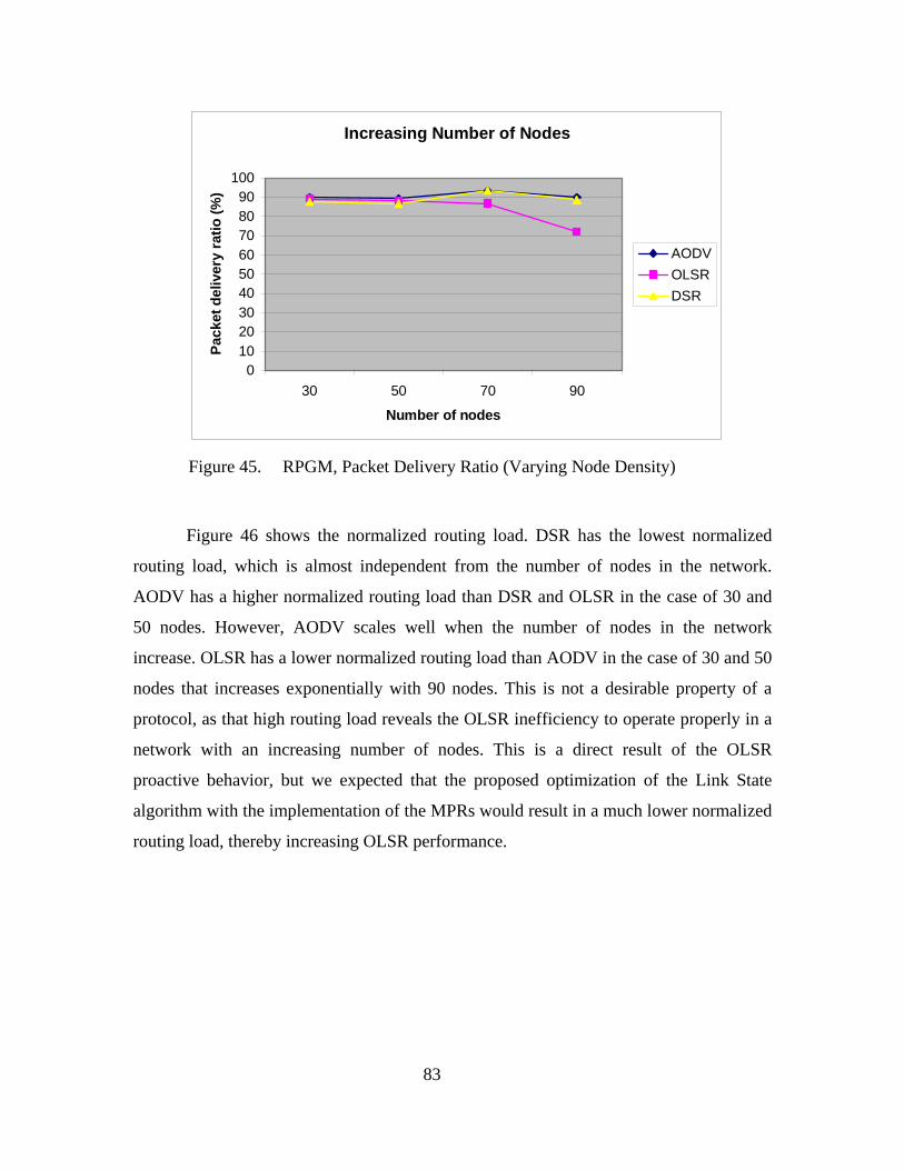
83
Increasing Number of Nodes
0102030405060708090
100
30 50 70 90
Number of nodes
Pack
et d
eliv
ery
ratio
(%)
AODVOLSRDSR
Figure 45. RPGM, Packet Delivery Ratio (Varying Node Density)
Figure 46 shows the normalized routing load. DSR has the lowest normalized
routing load, which is almost independent from the number of nodes in the network.
AODV has a higher normalized routing load than DSR and OLSR in the case of 30 and
50 nodes. However, AODV scales well when the number of nodes in the network
increase. OLSR has a lower normalized routing load than AODV in the case of 30 and 50
nodes that increases exponentially with 90 nodes. This is not a desirable property of a
protocol, as that high routing load reveals the OLSR inefficiency to operate properly in a
network with an increasing number of nodes. This is a direct result of the OLSR
proactive behavior, but we expected that the proposed optimization of the Link State
algorithm with the implementation of the MPRs would result in a much lower normalized
routing load, thereby increasing OLSR performance.

84
Increasing Number of Nodes
0
0.5
1
1.5
2
2.5
30 50 70 90
Number of nodes
Nor
mal
ized
rout
ing
load
AODVOLSRDSR
Figure 46. RPGM, Normalized Routing Load (Varying Node Density)
Figure 47 shows the normalized MAC load. OLSR has the lowest normalized
MAC load except in the case of 90 nodes, in which OLSR generates a higher number of
control packets. That high number of the normalized MAC load reveals that the network
is congested, not by data packets, as we keep the data rate constant, but from the routing
packets generated by OLSR. The direct result of a congested network is a high end-to-
end delay, which increases exponentially in the case of 90 nodes, as we see in Figure 48.
Both AODV and DSR present small fluctuations in terms of the end-to-end delay, but
generally, their performance is stable in all cases.

85
Increasing Number of Nodes
0123456789
10
30 50 70 90
Number of nodes
Nor
mal
ized
MA
Clo
adAODVOLSRDSR
Figure 47. RPGM, Normalized MAC Load (Varying Node Density)
Increasing number of Nodes
0
200
400
600
800
1000
1200
1400
1600
30 50 70 90
Number of nodes
Ave
rage
End
2End
del
ay(m
ilis)
AODVOLSRDSR
Figure 48. RPGM, End2End Delay (Varying Node Density)
B. MANHATTAN GRID MOBILITY MODEL
1. Varying the Number of Connections In the first set of simulations, we keep constant the data rate per connection and
increase the number of connections in the network. Under the Manhattan Grid mobility
model, we use the same size simulation area as in the RPGM model but divide that area

86
into blocks sized 100m by 100m. Thus, we approximate a small neighborhood in an
urban area in which mobile nodes operate. However, under that mobility scenario, we
reduce the number of connections and the data rate per connection, because the network
connectivity is lower than in the RPGM model due to the presence of blocks. While
experimenting with a higher number of connections than those we use in the simulation
set below, we observed that all protocols presented a very low performance, making any
comparison meaningless. Table 11 shows the chosen simulation parameters.
Table 11. Manhattan Grid, Varying the Number of Connections
Figure 49 shows the packet delivery ratio. The performance of the protocols is
much lower than in the RPGM model, even with the lower data rates per connection, and
the lower number of connections. The division of the simulation area into blocks
seriously affects the protocols’ performance. We observe that, unlike the RPGM model,
DSR has the highest packet delivery ratio, while OLSR presents the lowest packet
delivery ratio in both mobility models. The packet delivery ratio of AODV in the RPGM
model was higher than that of DSR. However, under the Manhattan grid mobility model,
the AODV performance is significantly lower than that of DSR.

87
Increasing Number of Connections
0
10
20
30
40
50
60
70
5 10 15 20
Number of connections
Pack
et d
eliv
ery
ratio
(%)
AODVOLSRDSR
Figure 49. Manhattan Grid, Packet Delivery Ratio (Increasing number of connections)
Figure 50 shows the normalized routing load of the protocols, which is higher
than that in the RPGM model by a factor of 10 for all protocols. DSR outperforms both
AODV and OLSR, while OLSR has the highest routing load, as expected. By analyzing
the simulation trace files, we found that AODV generates a higher number of RREQ and
RREP messages than DSR.
Figure 51 shows the normalized MAC load. The OLSR performance is the most
stable, due to its proactive behavior, while DSR outperforms AODV, except for the case
of 20 connections, unlike the RPGM model. Therefore, we can conclude that DSR can
perform better than AODV in networks with low connectivity. The low connectivity in
the Manhattan Grid model forces AODV to generate a higher number of routing control
messages, which results in a higher normalized MAC load.
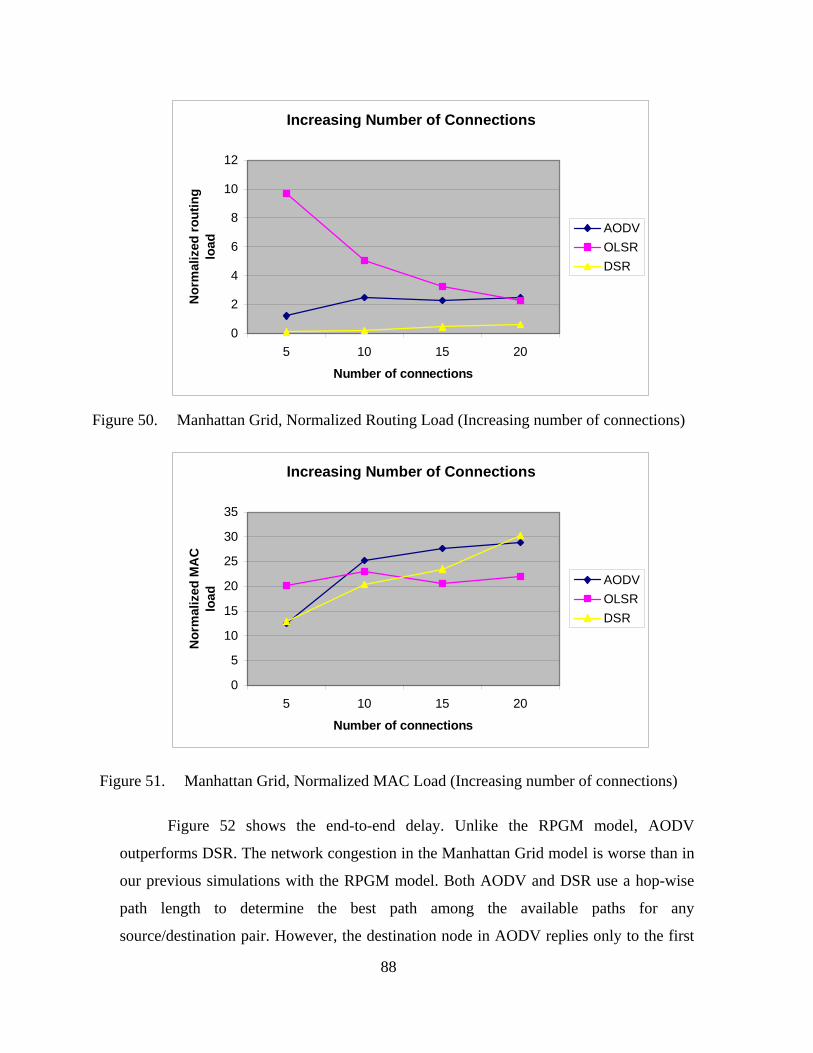
88
Increasing Number of Connections
0
2
4
6
8
10
12
5 10 15 20
Number of connections
Nor
mal
ized
rout
ing
load
AODVOLSRDSR
Figure 50. Manhattan Grid, Normalized Routing Load (Increasing number of connections)
Increasing Number of Connections
0
5
10
15
20
25
30
35
5 10 15 20
Number of connections
Nor
mal
ized
MA
Clo
ad
AODVOLSRDSR
Figure 51. Manhattan Grid, Normalized MAC Load (Increasing number of connections)
Figure 52 shows the end-to-end delay. Unlike the RPGM model, AODV
outperforms DSR. The network congestion in the Manhattan Grid model is worse than in
our previous simulations with the RPGM model. Both AODV and DSR use a hop-wise
path length to determine the best path among the available paths for any
source/destination pair. However, the destination node in AODV replies only to the first
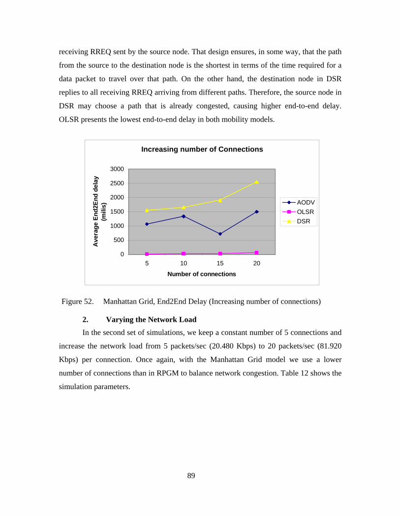
89
receiving RREQ sent by the source node. That design ensures, in some way, that the path
from the source to the destination node is the shortest in terms of the time required for a
data packet to travel over that path. On the other hand, the destination node in DSR
replies to all receiving RREQ arriving from different paths. Therefore, the source node in
DSR may choose a path that is already congested, causing higher end-to-end delay.
OLSR presents the lowest end-to-end delay in both mobility models.
Increasing number of Connections
0
500
1000
1500
2000
2500
3000
5 10 15 20
Number of connections
Ave
rage
End
2End
del
ay(m
ilis)
AODVOLSRDSR
Figure 52. Manhattan Grid, End2End Delay (Increasing number of connections) 2. Varying the Network Load
In the second set of simulations, we keep a constant number of 5 connections and
increase the network load from 5 packets/sec (20.480 Kbps) to 20 packets/sec (81.920
Kbps) per connection. Once again, with the Manhattan Grid model we use a lower
number of connections than in RPGM to balance network congestion. Table 12 shows the
simulation parameters.

90
Table 12. Manhattan Grid, Varying the Network load
Figure 53 shows the packet delivery ratio of the protocols. Like the RPGM model,
OLSR has the lowest packet delivery ratio, which, however, remains stable in all cases.
AODV outperforms DSR except for the case of 5 packets/sec.
DSR presents the lowest routing load (Figure 54), outperforming AODV and
OLSR. We have observed the same performance in all of our previous sets of simulations
with both mobility models. Although, at this point, we have not finished all of our
simulation sets, we can conclude that DSR is a more efficient protocol than AODV and
OLSR, in terms of the routing load and wireless medium utilization for data traffic in
networks with low mobility and a small number of nodes.
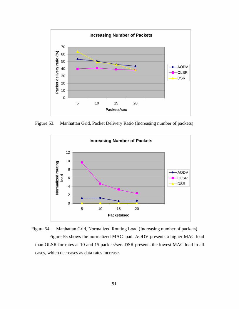
91
Increasing Number of Packets
0
10
20
30
40
50
60
70
5 10 15 20
Packets/sec
Pack
et d
eliv
ery
ratio
(%)
AODVOLSRDSR
Figure 53. Manhattan Grid, Packet Delivery Ratio (Increasing number of packets)
Increasing Number of Packets
0
2
4
6
8
10
12
5 10 15 20
Packets/sec
Nor
mal
ized
rout
ing
load
AODVOLSRDSR
Figure 54. Manhattan Grid, Normalized Routing Load (Increasing number of packets)
Figure 55 shows the normalized MAC load. AODV presents a higher MAC load
than OLSR for rates at 10 and 15 packets/sec. DSR presents the lowest MAC load in all
cases, which decreases as data rates increase.

92
Increasing Number of Packets
0
5
10
15
20
25
5 10 15 20
Packets/sec
Nor
mal
ized
MA
C lo
adAODVOLSRDSR
Figure 55. Manhattan Grid, Normalized MAC Load (Increasing number of packets)
Figure 56 shows the end-to-end delay. The superiority of OLSR in terms of end-
to-end delay is obvious. Both DSR and AODV have a higher end-to-end delay than
OLSR, by a factor that scales from 5 to 100.
Increasing Number of Packets
0200400600800
10001200140016001800
5 10 15 20
Packets/sec
Ave
rage
End
2End
del
ay(m
illis
) AODVOLSRDSR
Figure 56. Manhattan Grid, End2End Delay (Increasing number of packets)
By comparing the performance of AODV and DSR, we see that DSR presents a
generally higher end-to-end delay than AODV. The reason lies in the way that the
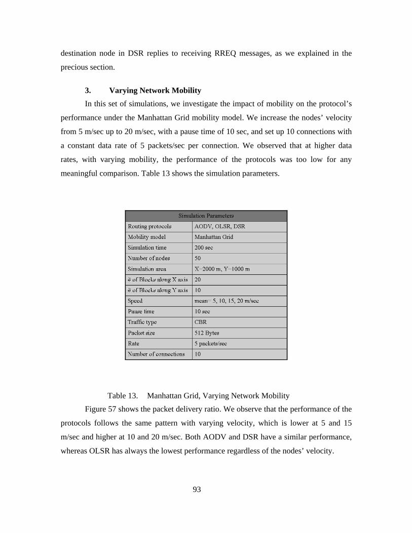
93
destination node in DSR replies to receiving RREQ messages, as we explained in the
precious section.
3. Varying Network Mobility In this set of simulations, we investigate the impact of mobility on the protocol’s
performance under the Manhattan Grid mobility model. We increase the nodes’ velocity
from 5 m/sec up to 20 m/sec, with a pause time of 10 sec, and set up 10 connections with
a constant data rate of 5 packets/sec per connection. We observed that at higher data
rates, with varying mobility, the performance of the protocols was too low for any
meaningful comparison. Table 13 shows the simulation parameters.
Table 13. Manhattan Grid, Varying Network Mobility
Figure 57 shows the packet delivery ratio. We observe that the performance of the
protocols follows the same pattern with varying velocity, which is lower at 5 and 15
m/sec and higher at 10 and 20 m/sec. Both AODV and DSR have a similar performance,
whereas OLSR has always the lowest performance regardless of the nodes’ velocity.

94
Increasing Network Mobility
0102030405060708090
5 10 15 20
Velocity in m/sec
Pack
et d
eliv
ery
ratio
(%)
AODVOLSRDSR
Figure 57. Manhattan Grid, Packet Delivery Ratio (Varying Network Mobility)
Figure 58 shows the normalized routing load. DSR outperforms OLSR and
AODV in all cases. Both AODV and DSR present a very stable normalized routing load,
while the OLSR normalized routing load is inverse proportional to the packet delivery
ratio. This phenomenon can be explained, by the way we calculate the normalized routing
load, as the fraction of all routing packets generated by the nodes over the number of all
received data packets. As the OLSR routing packets are not highly dependent on the
network topology, the fraction of the normalized routing load is inverse proportional to
the packet delivery ratio. The higher the packet delivery ratio, the lower the normalized
routing load.

95
Increasing Network Mobility
0
2
4
6
8
10
12
5 10 15 20
Velocity in m/sec
Nor
mal
ized
rout
ing
load
AODVOLSRDSR
Figure 58. Manhattan Grid, Normalized Routing Load (Varying Network Mobility)
Figure 59 shows the normalized MAC load. Both AODV and DSR have a similar
performance, while OLSR presents the highest normalized MAC load in all cases.
However, the protocol’s performance, in general, is worse by at least a factor of 2 when
compared to the RPGM model.
Increasing Network Mobility
0
5
10
15
20
25
30
35
5 10 15 20
Velocity in m/sec
Nor
mal
ized
MA
Clo
ad
AODVOLSRDSR
Figure 59. Manhattan Grid, Normalized MAC Load (Varying Network Mobility)
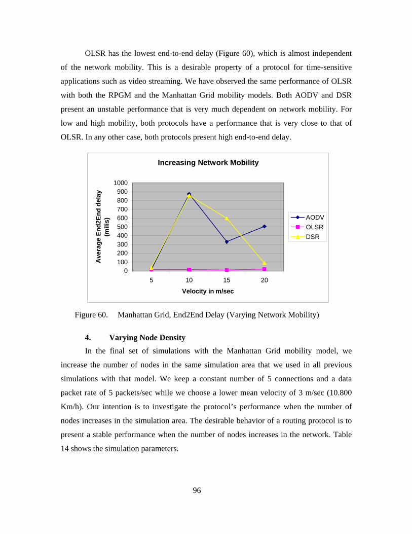
96
OLSR has the lowest end-to-end delay (Figure 60), which is almost independent
of the network mobility. This is a desirable property of a protocol for time-sensitive
applications such as video streaming. We have observed the same performance of OLSR
with both the RPGM and the Manhattan Grid mobility models. Both AODV and DSR
present an unstable performance that is very much dependent on network mobility. For
low and high mobility, both protocols have a performance that is very close to that of
OLSR. In any other case, both protocols present high end-to-end delay.
Increasing Network Mobility
0100200300400500600700800900
1000
5 10 15 20
Velocity in m/sec
Ave
rage
End
2End
del
ay(m
ilis)
AODVOLSRDSR
Figure 60. Manhattan Grid, End2End Delay (Varying Network Mobility)
4. Varying Node Density In the final set of simulations with the Manhattan Grid mobility model, we
increase the number of nodes in the same simulation area that we used in all previous
simulations with that model. We keep a constant number of 5 connections and a data
packet rate of 5 packets/sec while we choose a lower mean velocity of 3 m/sec (10.800
Km/h). Our intention is to investigate the protocol’s performance when the number of
nodes increases in the simulation area. The desirable behavior of a routing protocol is to
present a stable performance when the number of nodes increases in the network. Table
14 shows the simulation parameters.

97
Table 14. Manhattan Grid, Varying Node Density
Figure 61 shows the packet delivery ratio of the protocols. We observe that all
protocols follow the same pattern in all cases and present their best performance in the
case of 90 nodes. DSR and AODV have a similar performance, while OLSR presents the
worst performance. Once again, the periodic dissemination of HELO and link state
packets from OLSR creates a higher congestion in the network that results in a higher
number of dropped-data-packets events.
Figure 62 shows the normalized routing load. OLSR has the higher routing load in
all cases, while DSR outperforms AODV. DSR is the protocol with the most stable
behavior, regardless of the number of nodes in the network. This is a desirable property
for a routing protocol, as the routing overhead seems to be independent of the number of
nodes in the network.
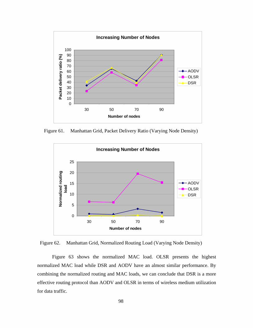
98
Increasing Number of Nodes
0102030405060708090
100
30 50 70 90
Number of nodes
Pack
et d
eliv
ery
ratio
(%)
AODVOLSRDSR
Figure 61. Manhattan Grid, Packet Delivery Ratio (Varying Node Density)
Increasing Number of Nodes
0
5
10
15
20
25
30 50 70 90
Number of nodes
Nor
mal
ized
rout
ing
load
AODVOLSRDSR
Figure 62. Manhattan Grid, Normalized Routing Load (Varying Node Density)
Figure 63 shows the normalized MAC load. OLSR presents the highest
normalized MAC load while DSR and AODV have an almost similar performance. By
combining the normalized routing and MAC loads, we can conclude that DSR is a more
effective routing protocol than AODV and OLSR in terms of wireless medium utilization
for data traffic.

99
Increasing Number of Nodes
0
5
10
15
20
25
30
35
40
30 50 70 90
Number of nodes
Nor
mal
ized
MA
Clo
ad
AODVOLSRDSR
Figure 63. Manhattan Grid, Normalized MAC Load (Varying Node Density)
Increasing number of Nodes
0
200
400
600
800
1000
1200
1400
30 50 70 90
Number of nodes
Ave
rage
End
2End
del
ay(m
ilis)
AODVOLSRDSR
Figure 64. Manhattan Grid, End2End Delay (Varying Node Density)
Finally, we observe in Figure 64 that OLSR has the lowest end-to-end delay,
which is independent of the number of nodes in the network. All routing protocols have
an identical performance in the case of 90 nodes, because the data packets are more
evenly distributed in the network. We observed the same phenomena in our previous
simulation with the RPGM model in a network with 70 nodes.

100
THIS PAGE INTENTIONALLY LEFT BLANK
101
V. CONCLUSIONS AND RECOMMENDATIONS FOR FUTURE WORK
This thesis discusses the evaluation of two reactive routing protocols, AODV and
DSR, and one proactive protocol, OLSR, based on simulation results with the network
simulator [NS-2]. One hundred and eight simulations under the Reference Point Group
Mobility (RPGM) and Manhattan Grid mobility models were conducted, and thirty
testing simulations, to choose the simulation parameters in a way that they allowed the
routing protocols to present a packet delivery ratio above 50 percent, in order to have
meaningful and comparable results. The goals were to better understand the limitations of
the tested protocols, to disclose design flaws, and to make recommendations for
optimizing their performance. The performance of the tested routing protocols depended
strongly on the above two mobility models and the simulation parameters chosen for each
simulation set. The thesis conclusions and recommendations for future work are
summarized below.
A. CONCLUSIONS OLSR had the lowest performance in terms of the packet delivery ratio in all of
the simulations with both the RPGM and the Manhattan grid mobility model. The reason
lies in the proactive behavior of OLSR, because the Multipoint Relay (MPR) nodes flood
the network with Topology Control (TC) packets every 5 seconds (default value).
Therefore, when the network load increases, data packets are dropped by the mobile
nodes due to network congestion caused by the periodic transmission of TC packets.
OLSR presented the lowest end-to-end delay in almost all of the simulations, and
in most cases, the end-to-end delay was independent of the varying simulation
parameters. OLSR is a good compromise when combining the protocol performance, in
terms of the packet delivery ratio and the end-to-end delay. It is concluded that, OLSR is
the most efficient protocol for time-sensitive applications such as voice and video
transmission. However, a few cases were observed in which OLSR had a higher end-to-
end delay than the other two reactive protocols (Figures 36 and 40). This is a direct result
of the high network congestion in certain areas of the network. By adjusting the TC
102
packet interval and the nodes’ willingness default values to the network attributes
(mobility, topology, number of nodes, transport protocol), one could reduce network
congestion and end-to-end delay.
AODV performance depended on the mobility models that were used in the
simulations. Under the RPGM model with low mobility, AODV has a lower packet
delivery ratio (Figures 29 and 33), higher normalized routing (Figures 30 and 34) and
MAC loads (Figures 31 and 35), and a higher end-to-end delay (Figures 32 and 36) than
DSR. In networks with a small number of nodes and low mobility, AODV does not
suggest a good solution as a routing protocol. However, AODV has better performance in
networks with higher mobility and a greater number of nodes. Simulation results in those
networks suggest that AODV presents a higher packet delivery ratio (Figure 41, Figure
45) and a lower normalized MAC load (Figures 43 and 47) than DSR and OLSR. In
addition, AODV performance in terms of end-to-end delay (Figures 44 and 48) is very
close to that of OLSR. It is concluded that AODV is the proper protocol for any kind of
application (voice, video, file transfer, etc.) in networks with high mobility that consist of
up to 90 or more nodes.
Under the Manhattan grid mobility model in a network with 50 nodes and low
mobility, AODV had a lower packet delivery ratio than DSR but a higher ratio than that
of OLSR (Figures 49 and 53). This classification among the three protocols also stands in
terms of the normalized routing and MAC loads (Figures 50, 51, 54, and 55). The striking
difference among the three protocols is the end-to-end delay, in which the OLSR
superiority is obvious (Figures 52 and 56). AODV improves its performance in networks
with a greater number of nodes and higher mobility, which, however, remains lower than
that of DSR. It is concluded that AODV is not the proper protocol in networks with low
connectivity, regardless of the network mobility and number of nodes.
With the RPGM reference model and a heavy network load, DSR presented the
best performance in terms of packet delivery ratio and end-to-end delay (Figures 33, 36).
In most cases, under this mobility model, DSR presented the lowest normalized routing
and MAC loads, proving that source routing proves to be an efficient routing mechanism

103
in networks with a small number of nodes and high connectivity, because it utilizes the
wireless medium for data traffic in a better way than the other tested protocols.
However, DSR performance decreases in networks with higher mobility (Figures
41, 44), disclosing that source routing cannot efficiently adapt the network topology
changes that are caused by the frequent movement of the mobility nodes. The same set of
observations was obtained when comparing DSR performance in networks with an
increasing number of nodes. Under this scenario, DSR presents lower performance than
AODV in terms of the packet delivery ratio and end-to-end delay (Figures 45, 48).
To summarize the above results and observations, it is concluded that DSR is a
good candidate as the routing protocol in networks with high connectivity, a small
number of nodes (up to 100), and low mobility. The high packet delivery ratio and the
low end-to-end delay in those networks enable the efficient use of time-sensitive
applications, such as voice and video streaming.
DSR presented the higher packet delivery ratio, under the Manhattan mobility
model, in a network with 50 nodes and a high number of connections, but its performance
in terms of end-to-end delay is poor and lower than that of OLSR and AODV (Figures
49, 52). When the mobility of the network increases, DSR presents almost the same
performance as AODV in terms of the packet delivery ratio and end-to-end delay. The
same results were observed with a higher number of nodes in the network under the
Manhattan mobility model.
It is concluded that DSR is not a good candidate as the routing protocol in
networks with low connectivity, regardless of the number of nodes and the network
mobility.
B. RECOMMENDATIONS FOR FUTURE WORK
1. Optimized Link State Routing (OLSR) It is recommended that further experiments be conducted on the value of the TC
packet interval to optimize the performance of OLSR when the attributes of the network
are known in advance. In a network with low mobility for instance, one should increase
the TC time interval, as network topology does not change so frequently and routing

104
tables have valid routes to any source/destination pair for a longer period. Alternatively,
in a network with high mobility, one should decrease the TC time interval, as network
topology changes more frequently and valid routes expire in short periods. In this way,
one could control the number of TC packets in the network, balancing network
congestion, and thereby optimizing OLSR performance.
A second optimization of the protocol is recommended by adjusting the nodes’
willingness value to reflect network topology. In the simulations of this thesis, the value
of the nodes’ willingness was set to 3, which is the default value in accordance with RFC
3626. That means that a node is willing to act as a MPR for all nodes within a distance of
3 hops away. In a cluster-like network, one can set that value in such a way that a node
will not act as an MPR for nodes that lie outside its cluster. Thus, one could reduce the
dissemination of OLSR control packets in the network, reducing network congestion and
optimizing OLSR performance.
2. Ad Hoc on Demand Distance Vector (AODV) The main design flaw of AODV is the high number of RREQ and RREP
messages, which are generated by the mobile nodes. That high number of messages
increases routing overhead in the network, which results in higher network congestion.
An optimization of the AODV protocol is recommended by adjusting the time-
out value, which is defined as ACTIVE_ROUTE_TIMEOUT in RFC 3561, for routes
that have previously been used by a node, to reflect a given network topology and
mobility. However, to do that, one should know in advance the network mobility and
topology, so that one can estimate the optimal time-out value by experimenting with
different time-out values. Generally, in networks with low mobility, a large time-out
value should be chosen, as network topology does not change so frequently, whereas a
small value is more suitable in networks with high mobility.
3. Dynamic Source Routing Protocol (DSR) The main disadvantage of the protocol is the high end-to-end delay, which is
caused by the way the mobile nodes reply to RREQ messages.
A modification of the protocol is recommended in the way the mobile nodes
reply to incoming RREQ messages. AODV design can be used as an approach to address

105
this particular problem, by forcing the mobile nodes to reply only to the first incoming
RREQ message sent by a node in the network. In this way, DSR can discover the least
congested path between a source/destination pair and therefore decrease end-to-end
delay. An additional benefit of this modification will be a better utilization of the wireless
medium, as a lower number of RREP messages will flow the network.
4. Trace Analysis Software
The main objective when creating this software was to provide an easy way to get
the desirable quantitative metrics for this thesis. [TraceGraph] is free software for
analyzing ns2 trace files and runs on top of [Matlab]. [TraceGraph] provides a sufficient
number of network metrics and graphics for analyzing routing protocol performance.
However, the [TraceGraph] running time was too high for analyzing large ns-2 trace files
and thus acted as a “bottleneck” in the whole simulation process.
The trace analysis software is a simple program written in Java programming
language and, in this first version, supports the analysis of old ns-2 trace files for the
three routing protocols that were evaluated in this thesis. A further extension of the
software can support any other routing protocol for MANETs and can calculate any
desirable quantitative metric.
5. General Recommendations for Routing Protocols for MANETS It is the author’s understanding, after studying the routing protocols and running
several simulations for this thesis, that there is no protocol that can be applied to all
"kinds" of networks. In other words, there is no routing protocol for MANETs that can
provide efficient routing to any size of network, commercial or military, with a small or
large number of nodes and varying network load and mobility. What is needed to be done
is to adjust these protocols to the network attributes. No protocol can be seen as the best
solution for all mobility and traffic models. The bottom line: When one knows in advance
the mobility of the nodes, the network topology, the degree of connectivity, the type of
the transport protocol ( UDP or TCP), and the application that is to be used (email, ftp,
video, voice, etc.), he can adjust the internal parameters of the protocol (route updates
interval, HELLO interval, etc.) to get the best performance of the protocol. Here is where
the problem for finding and standardizing just a single protocol, which can solve the
routing problem in MANETs, is located. None of the proposed protocols can be THE

106
solution to the routing problem. On the other hand, if one takes any of the proposed
routing protocols and adjust its internal parameters to network attributes, he will have a
very good protocol, but only for a specific network or similar networks.
A second approach would be a self-configurable routing protocol that would be
able to adjust its internal parameters to network attributes. This protocol would collect a
number of statistics, such as observed end-to-end delay, packet delivery ratio, node
velocity, degree of network connectivity etc. and would make decisions to adjust its
behavior and therefore optimize its performance.
All the work, recommendations and concepts in previous sections in chapter V are
left for evaluation and future work.

107
APPENDIX A SAMPLE TCL SCRIPT
##################################################################### # This is a sample tcl script for use in network simulator 2 # # Author: Georgios Kioumourtzis # # Date : Dec 14 2005 # ##################################################################### set val(chan) Channel/WirelessChannel ;#Channel Type set val(prop) Propagation/TwoRayGround ;# radio-propagation model set val(netif) Phy/WirelessPhy ;# network interface type set val(mac) Mac/802_11 ;# MAC type set val(ifq) Queue/DropTail/PriQueue ;# interface queue type set val(ll) LL ;# link layer type set val(ant) Antenna/OmniAntenna ;# antenna model set val(ifqlen) 250 ;# max packet in ifq set val(nn) 90 ;# number of mobile nodes set val(rp) OLSR ;# routing protocol set val(x) 2020 ;# X dimension set val(y) 2020 ;# Y dimension set val(cp) "cbr-50-05-05" ;# traffic scenario set val(sc) "man-90nodes.ns_movements" ;# mobility scenario set val(seed) 1.0 ;# random seed set val(stop) 100.0 ;# simulation time ##################################################################### # Control OLSR behavior from this script - commented lines are not # needed because those are default values # #Agent/OLSR set use_mac_ true #Agent/OLSR set debug_ false #Agent/OLSR set willingness 3 #Agent/OLSR set hello_ival_ 2 #Agent/OLSR set tc_ival_ 5 ##################################################################### ###################################################################### # Default settings ###################################################################### LL set mindelay_ 50us LL set delay_ 25us LL set bandwidth_ 0;# not used #Agent/Null set sport_ 0 #Agent/Null set dport_ 0 Agent/CBR set sport_ 0 Agent/CBR set dport_ 0 #Agent/TCPSink set sport_ 0 #Agent/TCPSink set dport_ 0 #Agent/TCP set sport_ 0 #Agent/TCP set dport_ 0 #Agent/TCP set packetsize 512 Mac/802_11 set dataRate_ 2Mb #Mac/802_11 set RTSThreshold 0

108
set AgentTrace ON set RouterTrace ON set MacTrace ON Queue/DropTail/PriQueue set Prefer_Routing_Protocols 1 ###################################################################### # Set values for the antenna position ,Tx and Rx gain ###################################################################### Antenna/OmniAntenna set X_ 0 Antenna/OmniAntenna set Y_ 0 Antenna/OmniAntenna set Z_ 1.5 Antenna/OmniAntenna set Gt_ 1.0 Antenna/OmniAntenna set Gr_ 1.0 ###################################################################### # Initialize the sharedMedia interface with parameters to make it # work like the 914MHz Lucent WaveLAN DSSS radio ###################################################################### Phy/WirelessPhy set CPThresh_ 10.0 Phy/WirelessPhy set CSThresh_ 1.559e-11 Phy/WirelessPhy set RXThresh_ 3.652e-10 Phy/WirelessPhy set Rb_ 2*1e6 Phy/WirelessPhy set Pt_ 0.2818 Phy/WirelessPhy set freq_ 914e+6 Phy/WirelessPhy set L_ 1.0 Phy/WirelessPhy set dataRate_ 2Mb puts "simulation time " puts $val(stop) ###################################################################### # Initialize Global Variables ###################################################################### set ns_ [new Simulator] #$ns_ use-scheduler Heap $ns_ use-scheduler List #$ns_ use-scheduler RealTime set tracefd [open olsr-50-05-05-90nodes.tr w] #$ns_ use-newtrace $ns_ trace-all $tracefd #set namtrace [open olsr-50-10-10-200sec.nam w] #$ns_ namtrace-all-wireless $namtrace $val(x) $val(y) ###################################################################### # set up topography object ###################################################################### set topo [new Topography] $topo load_flatgrid $val(x) $val(y) ###################################################################### # Create God ###################################################################### create-god $val(nn)

109
###################################################################### # Create channel #1 ###################################################################### set chan_1_ [new $val(chan)] #set chan_2_ [new $val(chan)] ###################################################################### # Create nodes ###################################################################### $ns_ node-config -adhocRouting $val(rp) \ -llType $val(ll) \ -macType $val(mac) \ -ifqType $val(ifq) \ -ifqLen $val(ifqlen) \ -antType $val(ant) \ -propType $val(prop) \ -phyType $val(netif) \ -topoInstance $topo \ -agentTrace ON \ -routerTrace ON \ -macTrace ON \ -movementTrace ON \ -channel $chan_1_ for {set i 0} {$i < $val(nn)} {incr i} { set node_($i) [$ns_ node] # set r_($i) [$node_($i) set ragent_] # $ns_ at 0.0 "$r_($i) radius 2.0" $node_($i) random-motion 0 } ###################################################################### # Define node movement model ###################################################################### puts "Loading connection pattern..." source $val(cp) ###################################################################### # Define traffic model ###################################################################### puts "Loading scenario file..." source $val(sc) ###################################################################### # Define node initial position in nam ###################################################################### for {set i 0} {$i < $val(nn)} {incr i} { $ns_ initial_node_pos $node_($i) 50 } ###################################################################### # Tell nodes when the simulation ends ###################################################################### for {set i 0} {$i < $val(nn)} {incr i} { $ns_ at $val(stop).0 "$node_($i) reset";

110
} $ns_ at $val(stop).002 "puts \"NS EXITING...\"; $ns_ halt" puts $tracefd "M 0.0 nn $val(nn) x $val(x) y $val(y) rp $val(rp)" puts $tracefd "M 0.0 sc $val(sc) cp $val(cp) seed $val(seed)" puts $tracefd "M 0.0 prop $val(prop) ant $val(ant)" puts "Starting Simulation..." $ns_ run

111
APPENDIX B SAMPLE NS-2 TRACE FILE
##################################################################### # This is a trace file generated by ns-2 during the simulation #
#####################################################################
M 0.0 nn 30 x 2020 y 2020 rp OLSR M 0.0 sc man-30nodes.ns_movements cp cbr-50-05-05 seed 1.0 M 0.0 prop Propagation/TwoRayGround ant Antenna/OmniAntenna M 0.00000 3 (1002.18, 210.00, 0.00), (998.56, 210.00), 2.96 M 0.00000 4 (1056.64, 310.00, 0.00), (1040.54, 310.00), 2.84 M 0.00000 5 (410.00, 258.41, 0.00), (410.00, 260.07), 2.87 M 0.00000 8 (910.00, 531.22, 0.00), (910.00, 532.33), 3.15 M 0.00000 11 (1118.74, 910.00, 0.00), (1110.00, 910.00), 2.77 M 0.00000 12 (67.42, 610.00, 0.00), (69.44, 610.00), 3.07 M 0.00000 13 (310.00, 41.17, 0.00), (310.00, 36.12), 3.25 M 0.00000 14 (1873.15, 1010.00, 0.00), (1878.45, 1010.00), 2.90 M 0.00000 16 (1010.00, 564.50, 0.00), (1010.00, 562.09), 2.90 M 0.00000 19 (210.00, 229.33, 0.00), (210.00, 232.34), 2.95 M 0.00000 20 (487.54, 210.00, 0.00), (487.26, 210.00), 2.82 M 0.00000 21 (178.76, 110.00, 0.00), (174.87, 110.00), 3.00 M 0.00000 25 (1385.89, 210.00, 0.00), (1388.85, 210.00), 3.14 s 0.000169789 _0_ RTR --- 0 OLSR 48 [0 0 0 0] ------- [0:255 -1:255 32 0] [1 0 [HELLO 0 0 0]] s 0.000824789 _0_ MAC --- 0 OLSR 100 [0 ffffffff 0 800] ------- [0:255 -1:255 32 0] [1 0 [HELLO 0 0 0]] r 0.001625368 _25_ MAC --- 0 OLSR 48 [0 ffffffff 0 800] ------- [0:255 -1:255 32 0] [1 0 [HELLO 0 0 0]] r 0.001625589 _2_ MAC --- 0 OLSR 48 [0 ffffffff 0 800] ------- [0:255 -1:255 32 0] [1 0 [HELLO 0 0 0]] r 0.001650368 _25_ RTR --- 0 OLSR 48 [0 ffffffff 0 800] ------- [0:255 -1:255 32 0] [1 0 [HELLO 0 0 0]] r 0.001650589 _2_ RTR --- 0 OLSR 48 [0 ffffffff 0 800] ------- [0:255 -1:255 32 0] [1 0 [HELLO 0 0 0]] s 0.044061336 _1_ RTR --- 1 OLSR 48 [0 0 0 0] ------- [1:255 -1:255 32 0] [1 0 [HELLO 1 0 0]] s 0.044316336 _1_ MAC --- 1 OLSR 100 [0 ffffffff 1 800] ------- [1:255 -1:255 32 0] [1 0 [HELLO 1 0 0]] r 0.045116854 _21_ MAC --- 1 OLSR 48 [0 ffffffff 1 800] ------- [1:255 -1:255 32 0] [1 0 [HELLO 1 0 0]] r 0.045141854 _21_ RTR --- 1 OLSR 48 [0 ffffffff 1 800] ------- [1:255 -1:255 32 0] [1 0 [HELLO 1 0 0]] s 0.045678458 _22_ RTR --- 2 OLSR 48 [0 0 0 0] ------- [22:255 -1:255 32 0] [1 0 [HELLO 22 0 0]] s 0.046193458 _22_ MAC --- 2 OLSR 100 [0 ffffffff 16 800] ------- [22:255 -1:255 32 0] [1 0 [HELLO 22 0 0]] r 0.046993798 _27_ MAC --- 2 OLSR 48 [0 ffffffff 16 800] ------- [22:255 -1:255 32 0] [1 0 [HELLO 22 0 0]] r 0.046993922 _6_ MAC --- 2 OLSR 48 [0 ffffffff 16 800] ------- [22:255 -1:255 32 0] [1 0 [HELLO 22 0 0]] r 0.046993930 _7_ MAC --- 2 OLSR 48 [0 ffffffff 16 800] ------- [22:255 -1:255 32 0] [1 0 [HELLO 22 0 0]] r 0.046994099 _26_ MAC --- 2 OLSR 48 [0 ffffffff 16 800] ------- [22:255 -1:255 32 0] [1 0 [HELLO 22 0 0]]

112
r 0.046994246 _20_ MAC --- 2 OLSR 48 [0 ffffffff 16 800] ------- [22:255 -1:255 32 0] [1 0 [HELLO 22 0 0]] r 0.047018798 _27_ RTR --- 2 OLSR 48 [0 ffffffff 16 800] ------- [22:255 -1:255 32 0] [1 0 [HELLO 22 0 0]] r 0.047018922 _6_ RTR --- 2 OLSR 48 [0 ffffffff 16 800] ------- [22:255 -1:255 32 0] [1 0 [HELLO 22 0 0]] r 0.047018930 _7_ RTR --- 2 OLSR 48 [0 ffffffff 16 800] ------- [22:255 -1:255 32 0] [1 0 [HELLO 22 0 0]] r 0.047019099 _26_ RTR --- 2 OLSR 48 [0 ffffffff 16 800] ------- [22:255 -1:255 32 0] [1 0 [HELLO 22 0 0]] r 0.047019246 _20_ RTR --- 2 OLSR 48 [0 ffffffff 16 800] ------- [22:255 -1:255 32 0] [1 0 [HELLO 22 0 0]] s 0.054599236 _12_ RTR --- 3 OLSR 48 [0 0 0 0] ------- [12:255 -1:255 32 0] [1 0 [HELLO 12 0 0]] s 0.054794236 _12_ MAC --- 3 OLSR 100 [0 ffffffff c 800] ------- [12:255 -1:255 32 0] [1 0 [HELLO 12 0 0]] s 0.056015658 _14_ RTR --- 4 OLSR 48 [0 0 0 0] ------- [14:255 -1:255 32 0] [1 0 [HELLO 14 0 0]] s 0.056310658 _14_ MAC --- 4 OLSR 100 [0 ffffffff e 800] ------- [14:255 -1:255 32 0] [1 0 [HELLO 14 0 0]] s 0.056904124 _5_ RTR --- 5 OLSR 48 [0 0 0 0] ------- [5:255 -1:255 32 0] [1 0 [HELLO 5 0 0]] s 0.056979124 _5_ MAC --- 5 OLSR 100 [0 ffffffff 5 800] ------- [5:255 -1:255 32 0] [1 0 [HELLO 5 0 0]] r 0.057110785 _10_ MAC --- 4 OLSR 48 [0 ffffffff e 800] ------- [14:255 -1:255 32 0] [1 0 [HELLO 14 0 0]] r 0.057135785 _10_ RTR --- 4 OLSR 48 [0 ffffffff e 800] ------- [14:255 -1:255 32 0] [1 0 [HELLO 14 0 0]] r 0.057779429 _20_ MAC --- 5 OLSR 48 [0 ffffffff 5 800] ------- [5:255 -1:255 32 0] [1 0 [HELLO 5 0 0]] r 0.057779508 _6_ MAC --- 5 OLSR 48 [0 ffffffff 5 800] ------- [5:255 -1:255 32 0] [1 0 [HELLO 5 0 0]] r 0.057779683 _27_ MAC --- 5 OLSR 48 [0 ffffffff 5 800] ------- [5:255 -1:255 32 0] [1 0 [HELLO 5 0 0]] r 0.057779798 _19_ MAC --- 5 OLSR 48 [0 ffffffff 5 800] ------- [5:255 -1:255 32 0] [1 0 [HELLO 5 0 0]] r 0.057779803 _26_ MAC --- 5 OLSR 48 [0 ffffffff 5 800] ------- [5:255 -1:255 32 0] [1 0 [HELLO 5 0 0]] r 0.057779922 _13_ MAC --- 5 OLSR 48 [0 ffffffff 5 800] ------- [5:255 -1:255 32 0] [1 0 [HELLO 5 0 0]] r 0.057804429 _20_ RTR --- 5 OLSR 48 [0 ffffffff 5 800] ------- [5:255 -1:255 32 0] [1 0 [HELLO 5 0 0]] r 0.057804508 _6_ RTR --- 5 OLSR 48 [0 ffffffff 5 800] ------- [5:255 -1:255 32 0] [1 0 [HELLO 5 0 0]] r 0.057804683 _27_ RTR --- 5 OLSR 48 [0 ffffffff 5 800] ------- [5:255 -1:255 32 0] [1 0 [HELLO 5 0 0]] r 0.057804798 _19_ RTR --- 5 OLSR 48 [0 ffffffff 5 800] ------- [5:255 -1:255 32 0] [1 0 [HELLO 5 0 0]] r 0.057804803 _26_ RTR --- 5 OLSR 48 [0 ffffffff 5 800] ------- [5:255 -1:255 32 0] [1 0 [HELLO 5 0 0]] r 0.057804922 _13_ RTR --- 5 OLSR 48 [0 ffffffff 5 800] ------- [5:255 -1:255 32 0] [1 0 [HELLO 5 0 0]] s 0.082072703 _4_ RTR --- 6 OLSR 48 [0 0 0 0] ------- [4:255 -1:255 32 0] [1 0 [HELLO 4 0 0]]

113
APPENDIX C SAMPLE TRAFFIC SCENARIO FILE
##################################################################### # This is a traffic scenario file generated by ns-2 #
##################################################################### # # nodes: 50, max conn: 5, send rate: 0.20000000000000001, seed: 1.0 # # # 1 connecting to 2 at time 2.5568388786897245 # set udp_(0) [new Agent/UDP] $ns_ attach-agent $node_(1) $udp_(0) set null_(0) [new Agent/Null] $ns_ attach-agent $node_(2) $null_(0) set cbr_(0) [new Application/Traffic/CBR] $cbr_(0) set packetSize_ 512 $cbr_(0) set interval_ 0.20000000000000001 $cbr_(0) set random_ 1 $cbr_(0) set maxpkts_ 10000 $cbr_(0) attach-agent $udp_(0) $ns_ connect $udp_(0) $null_(0) $ns_ at 2.5568388786897245 "$cbr_(0) start" # # 4 connecting to 5 at time 56.333118917575632 # set udp_(1) [new Agent/UDP] $ns_ attach-agent $node_(4) $udp_(1) set null_(1) [new Agent/Null] $ns_ attach-agent $node_(5) $null_(1) set cbr_(1) [new Application/Traffic/CBR] $cbr_(1) set packetSize_ 512 $cbr_(1) set interval_ 0.20000000000000001 $cbr_(1) set random_ 1 $cbr_(1) set maxpkts_ 10000 $cbr_(1) attach-agent $udp_(1) $ns_ connect $udp_(1) $null_(1) $ns_ at 56.333118917575632 "$cbr_(1) start" # # 4 connecting to 6 at time 146.96568928983328 # set udp_(2) [new Agent/UDP] $ns_ attach-agent $node_(4) $udp_(2) set null_(2) [new Agent/Null] $ns_ attach-agent $node_(6) $null_(2) set cbr_(2) [new Application/Traffic/CBR] $cbr_(2) set packetSize_ 512 $cbr_(2) set interval_ 0.20000000000000001 $cbr_(2) set random_ 1 $cbr_(2) set maxpkts_ 10000 $cbr_(2) attach-agent $udp_(2) $ns_ connect $udp_(2) $null_(2) $ns_ at 146.96568928983328 "$cbr_(2) start" #

114
# 6 connecting to 7 at time 55.634230382570173 # set udp_(3) [new Agent/UDP] $ns_ attach-agent $node_(6) $udp_(3) set null_(3) [new Agent/Null] $ns_ attach-agent $node_(7) $null_(3) set cbr_(3) [new Application/Traffic/CBR] $cbr_(3) set packetSize_ 512 $cbr_(3) set interval_ 0.20000000000000001 $cbr_(3) set random_ 1 $cbr_(3) set maxpkts_ 10000 $cbr_(3) attach-agent $udp_(3) $ns_ connect $udp_(3) $null_(3) $ns_ at 55.634230382570173 "$cbr_(3) start" # # 7 connecting to 8 at time 29.546173154165118 # set udp_(4) [new Agent/UDP] $ns_ attach-agent $node_(7) $udp_(4) set null_(4) [new Agent/Null] $ns_ attach-agent $node_(8) $null_(4) set cbr_(4) [new Application/Traffic/CBR] $cbr_(4) set packetSize_ 512 $cbr_(4) set interval_ 0.20000000000000001 $cbr_(4) set random_ 1 $cbr_(4) set maxpkts_ 10000 $cbr_(4) attach-agent $udp_(4) $ns_ connect $udp_(4) $null_(4) $ns_ at 29.546173154165118 "$cbr_(4) start" # #Total sources/connections: 4/5 #

115
APPENDIX D SIMULATION ANALYSIS PROGRAM SOURCE CODE
A. MAIN CLASS OF THE PROGRAM
/** * <p>Title: Trace File Analyzer</p> *<p>Description: This is a simple java program to analyze ns2 * trace files. </p> *<p>Copyright: Copyright (c) 2005</p> * @author Georgios Kioumourtzis * @version 1.0 */ /** * The main class of the program. */ class TraceAnalyzerMain { /** The object of ProcessData class */ private static ProcessData processData;
/** The main method of the program. It calls the top level method start() */
public static void main(String[] args) { start(); } /** * The top level method of the program. It calls all other * methods */ private static void start() { processData = new ProcessData(); processData.process(); processData.printSimulationStats(); } }
B. CLASS TRACE FILE import java.io.*; import javax.swing.JFileChooser; /** * This class opens the ns2 trace file, reads the file line by * line and saves the simulation results in an output file

116
*/ class TraceFile { //--------------------------------------------------------------- // Data Members //--------------------------------------------------------------- /** The constant for empty string */ private static final String EMPTY_STRING = ""; /** The generic filepath separator */
private static String fileSeparator = System.getProperty("file.separator");
/** The generic line terminator */
private static String lineTerminator = System.getProperty("line.separator");
/** The object for buffered reader */ private BufferedReader bufReader; //--------------------------------------------------------------- // Constructor //--------------------------------------------------------------- /** * Default constructor */ public TraceFile() { bufReader = null; } /** * Opens a file for input. * @throw IOException */ public void open() throws IOException { JFileChooser chooser = new
JFileChooser(System.getProperty("user.dir")); int reply = chooser.showOpenDialog(null); if (reply == JFileChooser.APPROVE_OPTION) { open(chooser.getSelectedFile().getAbsolutePath()); } } /** * Opens the designated textfile. * @param filename name of the textfile to open * @throw IOException */ public void open(String filename) throws IOException { File inFile = new File(filename);

117
FileReader fileReader = new FileReader(inFile); bufReader = new BufferedReader(fileReader); } /** * Returns the next line of input as a string. If * the end of file is reached, an empty string * is returned. * @return the next line of input string * @throw IOException when the file is not open */ public String readNext() throws IOException { if (bufReader == null) { throw new IOException("File is not opened yet"); } String line = bufReader.readLine(); if (line == null) { line = ""; } return line; } /** * Save the data to a text file. The file to save * the data is selected via a file chooser dialog. * @param data text data to be saved * @exception IOException */ public void save(String data) throws IOException { JFileChooser chooser = new
JFileChooser(System.getProperty("user.dir")); int reply = chooser.showSaveDialog(null); if (reply == JFileChooser.APPROVE_OPTION) { save(chooser.getSelectedFile().getAbsolutePath(),
data); } } /** * Saves the data to the designated textfile. * @param data to be saved * @param filename the file to be saved * @exception IOException */ public void save(String filename, String data) throws
IOException { File outFile = new File(filename); FileOutputStream outFileStream = new
FileOutputStream(outFile); PrintWriter outStream = new PrintWriter(outFileStream); outStream.print(data); outStream.close(); }

118
}
C. CLASS FILE ANALYZER import java.awt.List; import java.io.IOException; import java.util.StringTokenizer; import java.util.regex.Matcher; import java.util.regex.Pattern; /** This class analyzes the results of the ns2 trace file. It * uses mainly the Pattern and Matcher classes and creates two * Lists (Received packet list and Send Packet List). From these * two lists we further process the data of the ns2 trace file */ public class FileAnalyzer { //--------------------------------------------------------------- // Data Members //--------------------------------------------------------------- /** The object of the Pattern class */ Pattern pat; /** The object of the Matcher class */ Matcher mat; /** The Default agent type */ private static final String DEFAULT_AGENT = "NONE"; /** The String to hold the agent type*/ String agent; /** The object to open and read the ns2 trace file */ TraceFile trFile; /** The number of sent data packets */ private int sentPkts; /** The number of received data packets */ private int rcvPkts;
/** The object to create a List of the sent data packets. * We keep two important values. The data packet sequence * number and the time that the packet was sent by the Agent (AGT) */
List sentPktList; /** The object to create a List of the received data packets. * We keep two important values. The data packet sequence * number and the time that the packet received by the Agent * (AGT)*/

119
List rcvPktList; /** The routing packets (REQUEST, REPLY, ERROR) generated * by the AODV routing protocol */ private int generatedAODVPkts; /** The routing packets generated * by the DSR routing protocol */ private int generatedDSRkts; /** The routing packets (HELO,TC) generated * by the OLSR routing protocol */ private int generatedOLSRPkts; /** The MAC layer packets generated by the nodes. * They include ARP,CTS,RTS, and ACK packets. */ private int generatedMACPkts; /** The number of total drop data packts and the MAC and * the Network Layers */ private int droppedPkts; /** The number of forwarded data packets by the Routing Agent */ private int frwPkts; StringBuilder strBuilder; private double bytesSent; private double bytesReceived = 0.0; //----------------------------------------------------------- // Constructor //--------------------------------------------------------------- /** * The constructor of the class */ public FileAnalyzer() { trFile = new TraceFile(); sentPktList = new List(); rcvPktList = new List(); strBuilder = new StringBuilder(); generatedAODVPkts = 0; generatedDSRkts = 0; generatedOLSRPkts = 0; generatedMACPkts = 0; droppedPkts = 0; frwPkts = 0; try { jbInit(); } catch (Exception ex) { ex.printStackTrace();

120
} } //--------------------------------------------------------------- // Public Methods //--------------------------------------------------------------- /** This method starts the functions of the class * FileAnalyzer */
public void analyze() { readData(); } /** * The Getter method for the total number of received * data packets by all nodes * @return the total number of received data packets by * all nodes */ public int getRcvPkts() { return this.rcvPkts; } /** * The Getter method for the total number of sent * data packets by all nodes * @return the total number of sent data packets by all nodes */ public int getSentPkts() { return this.sentPkts; } /** * The Getter method for the total number of AODV routing * packets * @return the total number of AODV data packets generated * by all nodes */ public int getGeneratedAODVPkts() { return generatedAODVPkts; } /** * The Getter method for the total number of ZRP routing * packets * @return the total number of AODV data packets generated * by all nodes */ public int getGeneratedDSRkts() { return generatedDSRkts; }

121
/** * The Getter method for the total number of OLSR * routing packets * @return the total number of AODV data packets generated * by all nodes */ public int getGeneratedOLSRPkts() { return generatedOLSRPkts; } /** * The Getter method for the total number of MAC * layer packets * @return the total number of AODV data packets generated * by all nodes */ public int getGeneratedMACPkts() { return generatedMACPkts; } /** * The Getter method for the total number of drop * data packets by all nodes * @return the total number of drop data packets by all nodes */ public int getDroppedPkts() { return droppedPkts; } /** * The Getter method for the total number of forwarded * data packets by all nodes * @return the total number of forwarded data packets by * all nodes */ public int getFrwPkts() { return frwPkts; } public double getBytesSent() { return bytesSent; } public double getBytesReceived() { return bytesReceived; } /** * The Getter method for the send data packet list * @return the list of the send data packets */ public List getSentList() { return this.sentPktList; }

122
/** * The Getter method for the received data packet list * @return the list of the received data packets */ public List getRcvList() { return this.rcvPktList; } /** * The Getter method for the number of items in the * send packet list * @return the number of items in the list */ public int countItemsinSentList() { int count = sentPktList.getItemCount(); return count; } /** * The Getter method for the number of items in the * received packet list * @return the number of items in the list */ public int countItemsinRcvList() { int count = rcvPktList.getItemCount(); return count; } public void printFileHeader() { System.out.println(strBuilder.toString()); } //--------------------------------------------------------------- // Private Methods //--------------------------------------------------------------- /** * This method analyzes the ns2 trace file and adds * the results found in the trace file to received * packets list and sent packets list. It also * analyzes the events in the trace file at the AGT, * network and MAC layers. */ private void readData() { String line = ""; int sentRouteAODV_REQUEST = 0; int sentRouteAODV_REPLY = 0; int sentRouteAODV_ERROR = 0; int sentRouteDSR = 0; int generatedARPPkts = 0; int generatedCTSPkts = 0; int generatedRTSPkts = 0; int generatedACKPkts = 0; int countLines = 0; //open and read the trace file
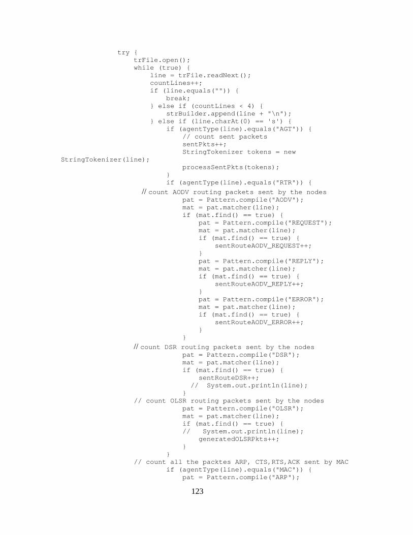
123
try { trFile.open(); while (true) { line = trFile.readNext(); countLines++; if (line.equals("")) { break; } else if (countLines < 4) { strBuilder.append(line + "\n"); } else if (line.charAt(0) == 's') { if (agentType(line).equals("AGT")) { // count sent packets sentPkts++; StringTokenizer tokens = new
StringTokenizer(line); processSentPkts(tokens); } if (agentType(line).equals("RTR")) { // count AODV routing packets sent by the nodes pat = Pattern.compile("AODV"); mat = pat.matcher(line); if (mat.find() == true) { pat = Pattern.compile("REQUEST"); mat = pat.matcher(line); if (mat.find() == true) { sentRouteAODV_REQUEST++; } pat = Pattern.compile("REPLY"); mat = pat.matcher(line); if (mat.find() == true) { sentRouteAODV_REPLY++; } pat = Pattern.compile("ERROR"); mat = pat.matcher(line); if (mat.find() == true) { sentRouteAODV_ERROR++; } } // count DSR routing packets sent by the nodes pat = Pattern.compile("DSR"); mat = pat.matcher(line); if (mat.find() == true) { sentRouteDSR++; // System.out.println(line); } // count OLSR routing packets sent by the nodes pat = Pattern.compile("OLSR"); mat = pat.matcher(line); if (mat.find() == true) { // System.out.println(line); generatedOLSRPkts++; } }
// count all the packtes ARP, CTS,RTS,ACK sent by MAC if (agentType(line).equals("MAC")) { pat = Pattern.compile("ARP");
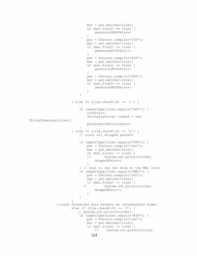
124
mat = pat.matcher(line); if (mat.find() == true) { generatedARPPkts++; } pat = Pattern.compile("CTS"); mat = pat.matcher(line); if (mat.find() == true) { generatedCTSPkts++; } pat = Pattern.compile("RTS"); mat = pat.matcher(line); if (mat.find() == true) { generatedRTSPkts++; } pat = Pattern.compile("ACK"); mat = pat.matcher(line); if (mat.find() == true) { generatedACKPkts++; } } } else if (line.charAt(0) == 'r') { if (agentType(line).equals("AGT")) { rcvPkts++; StringTokenizer tokens = new
StringTokenizer(line); processRcvPkts(tokens); } } else if (line.charAt(0) == 'D') { // count all dropped packets if (agentType(line).equals("RTR")) { pat = Pattern.compile("cbr"); mat = pat.matcher(line); if (mat.find() == true) { // System.out.println(line); droppedPkts++; } } // test to see cbr drop at the MAC level if (agentType(line).equals("MAC")) { pat = Pattern.compile("cbr"); mat = pat.matcher(line); if (mat.find() == true) { // System.out.println(line); droppedPkts++; } } } //count Forwarded Data Packets by intermediate nodes else if (line.charAt(0) == 'f') { // System.out.println(line); if (agentType(line).equals("RTR")) { pat = Pattern.compile("cbr"); mat = pat.matcher(line); if (mat.find() == true) { // System.out.println(line);

125
frwPkts++; } } } } } catch (IOException e) { System.out.println("Error reding input"); } generatedMACPkts = generatedARPPkts + generatedCTSPkts + generatedRTSPkts + generatedACKPkts; generatedAODVPkts = sentRouteAODV_REQUEST +
sentRouteAODV_REPLY + sentRouteAODV_ERROR; generatedDSRkts = sentRouteDSR; } /** * agentType * @param str String, the line of the trace file for * further analysis * @return String, the name of the agent (AGT,RTR,MAC) */ private String agentType(String str) { agent = DEFAULT_AGENT; pat = Pattern.compile("AGT"); mat = pat.matcher(str); if (mat.find() == true) { agent = "AGT"; } pat = Pattern.compile("RTR"); mat = pat.matcher(str); if (mat.find() == true) { agent = "RTR"; } pat = Pattern.compile("MAC"); mat = pat.matcher(str); if (mat.find() == true) { agent = "MAC"; } return agent; } /** * This method takes a line of the ns2 trace file in tokens * and add the values time and cbr sequence number into * the Received packet List. * @param tokens StringTokenizer, the line of the ns2 * trace file in tokens */ private void processRcvPkts(StringTokenizer tokens) { int size = tokens.countTokens(); String rcvInfo[] = new String[size]; for (int i = 0; i < size; i++) { //System.out.println(tokens.nextToken());

126
rcvInfo[i] = tokens.nextToken(); } // get the sequence number of the received packet rcvPktList.add(rcvInfo[1]); rcvPktList.add(rcvInfo[5]); bytesReceived+=Double.parseDouble(rcvInfo[7]); } /** * This method takes a line of the ns2 trace file in tokens * and adds the values time and cbr sequence number into * the Sent packet List. * @param tokens StringTokenizer, the line of the ns2 * trace file in tokens */ private void processSentPkts(StringTokenizer tokens) { int size = tokens.countTokens(); // System.out.println(size); // System.out.println(count_sent); String sentInfo[] = new String[size]; for (int i = 0; i < size; i++) { //System.out.println(tokens.nextToken()); sentInfo[i] = tokens.nextToken(); } // get the sequence number of the sent packet sentPktList.add(sentInfo[1]); sentPktList.add(sentInfo[5]); bytesSent+=Double.parseDouble(sentInfo[7]); } /** * jbInit * * @throws Exception */ private void jbInit() throws Exception { } } // end of class FileAnalyzer
D. CLASS PROCESS DATA package traceanalyzer; import java.awt.List; /** * The class to calculate the results given by the FileAnalyzer * class */ class ProcessData {
127
//--------------------------------------------------------------- // Data Members //--------------------------------------------------------------- /** * The object of the FileAnalyzer class to provide the * results of the trace file */ FileAnalyzer fileAnalyzer; /** * The packet Delivery Ratio that is (Received data * packets/sent data * packets) * 100 */ private double PDR; /** * The position in the delayArray to add a new value */ private int index; /** * An Array to keep the values of the simulation delay */ private double[] delayArray; /** * The total number of sent data packets by all nodes */ private double sentPkts; /** * The total number of received data packets by all nodes */ private double rcvPkts; //--------------------------------------------------------------- // Constructor //--------------------------------------------------------------- /** * The constructor of this class. */ public ProcessData() { fileAnalyzer = new FileAnalyzer(); sentPkts = 0.0; rcvPkts = 0.0; PDR = 0.0; index = 0; }

128
//--------------------------------------------------------------- // Public Methods //--------------------------------------------------------------- /** * This is the top level method of the class. It calls all * other private methods */ public void process() { fileAnalyzer.analyze(); int size = fileAnalyzer.getRcvPkts(); delayArray = new double[size]; PDR(); calculateDelay(); } /** * The method to print out the simulation results */ public void printSimulationStats() { fileAnalyzer.printFileHeader(); System.out.println("Sent Data Packets = " + sentPkts); System.out.println("Receive Data Packets = " + rcvPkts); double dropPkts = (double) fileAnalyzer.getDroppedPkts(); int frwPkts = fileAnalyzer.getFrwPkts(); System.out.println("Forward Data Packets = " + frwPkts); System.out.println("Drop Data Packets = " + dropPkts); System.out.println( "Data Packet Delivery Ratio (Received Pkts/Send
Pkts) = " + PDR + " %"); int AODVPkts = fileAnalyzer.getGeneratedAODVPkts(); int OLSRPkts = fileAnalyzer.getGeneratedOLSRPkts(); int DSRPkts = fileAnalyzer.getGeneratedDSRkts(); int MACPkts = fileAnalyzer.getGeneratedMACPkts(); int totalRoutingPackets = (AODVPkts + OLSRPkts +
DSRPkts); double normalizedRoutingLoad = totalRoutingPackets /
rcvPkts; int totalRoutingAndMACPkts = AODVPkts + OLSRPkts +
DSRPkts + MACPkts; double normalizedMACload = totalRoutingAndMACPkts /
rcvPkts; System.out.println("AODV Routing Packets = " + AODVPkts); System.out.println("OLSR Routing Packets = " + OLSRPkts); System.out.println("DSR Routing Packets = " + DSRPkts); System.out.println("MAC Packets (ARP, ACK, CTS, RTS) = "
+ MACPkts); System.out.println("Normalized Routing Load = " +
normalizedRoutingLoad); System.out.println("Normalized MAC load = " +
normalizedMACload); End2EndDelayStatistics(); System.out.println("Bytes sent = "+
fileAnalyzer.getBytesSent()); System.out.println("Bytes received = "+
fileAnalyzer.getBytesReceived()); }

129
//--------------------------------------------------------------- // Private Methods //--------------------------------------------------------------- /** * The method to calculate the packet delivery ratio */ private void PDR() { sentPkts = (double) fileAnalyzer.getSentPkts(); rcvPkts = (double) fileAnalyzer.getRcvPkts(); PDR = (rcvPkts / sentPkts) * 100; } /** * The method to calculate the delay between the time the * data packet send by the originator node and the time the * data packet received by the destination node. It writes * the result in an Array. The total number of received data * packets defines the size of the Array */ private void calculateDelay() { List sentList = new List(); List rcvList = new List(); sentList = fileAnalyzer.getSentList(); rcvList = fileAnalyzer.getRcvList(); double sentTime = 0; double rcvTime = 0; double delay = 0; int sentPktListSize = sentList.getItemCount(); int rcvPktListSize = rcvList.getItemCount(); for (int i = 0; i < sentPktListSize; i++) { sentTime = Double.parseDouble(sentList.getItem(i)); i++; int sent_pkt_sequence_number =
Integer.parseInt(sentList.getItem(i)); for (int j = 1; j < rcvPktListSize; j++) { int rcv_pkt_sequence_number =
Integer.parseInt(rcvList.getItem(j)); if (sent_pkt_sequence_number ==
rcv_pkt_sequence_number) { rcvTime =
Double.parseDouble(rcvList.getItem(j - 1)); delay = rcvTime - sentTime; addDelay(delay); } j++; } } }

130
/** * This method adds an element in the Array * @param delay the time the data packet received by the * destination node minus the time the data packet sent by * the originator node */ private void addDelay(double delay) { delayArray[index] = delay; index++; } /** * This method calculates the minimun, the maximun and the * average delays */ private void End2EndDelayStatistics() { double min = delayArray[0]; for (int i = 1; i < delayArray.length; i++) { if (delayArray[i] < min) { min = delayArray[i]; } } System.out.println("Minimun End2End Delay = " + min *
1000 + " milis"); double max = delayArray[0]; for (int i = 1; i < delayArray.length; i++) { if (delayArray[i] > max) { max = delayArray[i]; } } System.out.println("Maximun End2End Delay = " + max *
1000 + " milis"); double sum = 0; double averageDelay = 0; for (int i = 0; i < delayArray.length; i++) { sum += delayArray[i]; } averageDelay = sum / delayArray.length; System.out.println("Average End2End Delay = " +
averageDelay * 1000 + " milis"); } /** * The Getter method for all sent data packets by the nodes * @return double, the number of all sent data packets. */ public double getSentPkts() { return sentPkts; } /** * The Getter method for all received data packets by the * nodes * @return double, the number of all received data packets by * the nodes */ public double getRcvPkts() {

131
return rcvPkts; } /** * The Getter method for packet delivery Ratio * @return double, the packet delivery ratio (PDR) */ public double getPDR() { return PDR; } }

132
THIS PAGE INTENTIONALLY LEFT BLANK

133
LIST OF REFERENCES
[RFC 2501] S. Corson, J. Macker. Mobile Ad hoc Networking (MANET): Routing Protocol Performance Issues and Evaluation Considerations,
January 1999. [RFC 3626] T. Clausen, Ed., P. Jacquet, Ed. Project Hipercom, “Optimized Link
State Routing Protocol”, Project Hipercom, INRIA, October 2003. [Perkins 1994] C. E. Perkins and P. Bhagwat “Highly Dynamic Destination-
Sequenced Distance-Vector Routing (DSDV) for Mobile Computers,” Computer Communications Review, October 1994, pp. 234-244.
C.-C. Chiang, H-K. Wu, W.Liu, and M.Gerla 1997] C.-C.Chiang, H-K. Wu,
W.Liu and M.Gerla “Routing in Clustered Multihop, Mobile Wireless Networks with Fading Channel”, in Proceedings of IEEE Singapore International Conference on Networks (SICON), pages 197-211, April 1997.
[Wang 2003] Weichao Wang, Yi Lu, Bharat K. Bhargava, On Security Study of
Two Distance Vector Routing Protocols for Mobile Ad Hoc Networks. [RFC 3561] C. Perkins, E. Belding-Royer, S. Das. Ad hoc On-Demand
Distance Vector (AODV) Routing, July 2003. [M. G. Zapata 2004] Manel Guerrero Zapata, Secure Ad hoc On-Demand
Distance Vector (SAODV) Routing, MANET Internet draft :draft-guerrero- manet-saodv-02.txt, November 2004.
[Johnson, Matlz, and Hu 2004] D.B Johnson, D.A Maltz, and Yih-Chun Hu.
The Dynamic Source Routing Protocol for Mobile Ad Hoc Networks (DSR), Internet draft (draft-ietf-manet-dsr-10.txt), 19 July 2004.
[S. Buchegger, J.-Y. Le Boudec 2002] S. Buchegger, J.-Y. Le Boudec,
Performance Analysis of the CONFIDANT Protocol, (Cooperation Of Nodes: Fairness In Dynamic Ad-hoc Networks). Proceedings of the 3rd ACM international symposium on Mobile ad hoc networking & computing June 2002, Pages 226-236.
[V.D. Park and M.S. Corson 2001] V. D. Park, and M. S. Corson, “Temporally-
ordered routing algorithm (TORA) version 1 functional specification”, IETF Draft: draft-ietf-manet-tora-spec-04.txt, 2001.
[V.D. Park, J.P Macker, and M.S. Corson 1998] V.D. Park, J.P Macker, and
M.S. Corson 98, “Applicability of the Temporally-Ordered Routing Algorithm for use in Mobile Tactical Networks” Proceedings of IEEE MILCOM 1998.

134
[S. Corson, S. Papademetriou, P. Papadopoulos, V. Park, and A. Qayyum 1999] S. Corson, S. Papademetriou, P. Papadopoulos, V. Park, and A. Qayyum, “An Internet MANET encapsulation protocol (IMEP) specification”, IETF Draft: draft-ietfmanet- imep-spec02.txt, 1999.
[A. A. Pirzada, C. McDonald 2004], Asad Amir Pirzada, ChrisMcDonald,
“Trusted Route Discovery with TORA Protocol” Proceedings of the Second Annual Conference on Communication Networks and Services Research (CNSR’04).
[Haas, Z.J., Pearlman, M.R. and Samar, P 2003], Zygmunt J. Haas,
Marc R. Pearlman, Prince Samar, “The Zone Routing Protocol (ZRP) for Ad Hoc Networks”, <draft-ietf-manet-zone-zrp-04.txt>.
[Haas, Z.J., Pearlman, M.R. and Samar, P 2002], Zygmunt J. Haas,
Marc R. Pearlman, Prince Samar, “Intrazone Routing Protocol (IARP)," IETF Internet Draft, draft-ietf-manet-iarp-02.txt, July 2002.
[Haas, Z.J., Pearlman, M.R. and Samar, P 2002], Zygmunt J. Haas,
Marc R. Pearlman, Prince Samar, "Interzone Routing Protocol (IERP)," IETF Internet Draft, draft-ietf-manet-ierp-02.txt, July 2002. [Haas, Z.J., Pearlman, M.R. and Samar, P 2002], Zygmunt J. Haas, Marc R. Pearlman, Prince Samar, "Bordercasting Resolution Protocol (BRP)," IETF Internet Draft, draft-ietf-manet-brp-02.txt, July 2002.
[Carp and Kung 2000], B.Carp and H.T.Kung, “GPSR: Greedy Perimeter Statelles Routing for Wireless Networks” Proceedings of the sixth annual ACM/IEEE International Conference on Mobile Computing and Networking (MobiCom 2000).
[ZRP code], the source code for Zone Routing Protocol source code for ns-2 can be downloaded from: http://people.ece.cornell.edu/~haas/wnl/wnlprojects.html, accessed on December 2004. [NS-2], Network Simulator 2, the source code of ns2-allinone-2.28 can be downloaded from: http://www.isi.edu/nsnam/ns/ns-build.html, accessed on February 2005. [REAL Network Simulator], REAL 5.0 Overview http://www.cs.cornell.edu/skeshav/real/overview.html, accessed on February 2005. [FEDORA], The Fedora Project can be downloaded from http://fedora.redhat.com/, accessed on December 2004.

135
[UM-OLSR], the source code for OLSR of ns-2 version 2.28 can be downloaded from: http://ants.dif.um.es/masimum/um-olsr/um-olsr_ns-2.28_v0.8.7.patch, accessed on February 2005. [Waal 2003] Christian de Waal and Michael Gerharz. “BonnMotion: A Mobility Scenario Generation and Analysis Tool.” Communication Systems Group, Institute of Computer Science IV, University of Bonn, Germany. Bonnmotion-1.3 can be downloaded from : http://web.informatik.uni-bonn.de/IV/Mitarbeiter/dewaal/BonnMotion/, accessed on February 2005. [Hong 1999] X. Hong, M. Gerla, G. Pei and C.C. Chiang. “A Group Mobility Model for Ad Hoc Wireless Networks,” Proceeding of the 2nd ACM/IEEE Int. Workshop on Modeling and Simulation of Wireless and Mobile Systems (MSWiM'99), 1999, pp. 53-60. [Das, S.R., Perkins, C.E. Royer, E.M.2000], “Performance comparison of two on-demand routing protocols for ad hoc networks “, INFOCOM 2000. Nineteenth Annual Joint Conference of the IEEE Computer and Communications Societies. Proceedings. IEEEVolume 1, 26-30 March 2000 Page(s): 3 - 12 vol.1. [Amitabh Mishra, Ketan M. Nadkarni], “Security in Wireless Ad Hoc Networks”, Virginia Polytechnic Institute and State University. [TraceGraph], Trace graph can de downloaded from: http://www.geocities.com/tracegraph/, accessed on February 2005. [Matlab], the official web page of Matlab can de found in: http://www.mathworks.com/, accessed on March 2005. [Lee Kok Thong], “Performance Analysis of Mobile Ad Hoc Networking Routing Protocols” MS Thesis, NPS December 2004.

136
THIS PAGE INTENTIONALLY LEFT BLANK

137
INITIAL DISTRIBUTION LIST
1. Defense Technical Information Center Ft. Belvoir, Virginia
2. Dudley Knox Library Naval Postgraduate School Monterey, California
3. Dan Boger Department of Information Sciences Naval Postgraduate School Monterey, California
4. Peter J. Denning Department of Computer Science Naval Postgraduate School
Monterey, California
5. Gilbert M. Lundy Department of Computer Science Naval Postgraduate School
Monterey, California
6. Rex Bunddenberg Department of Information Sciences Naval Postgraduate School Monterey, California
7. Georgios Kioumourtzis Hellenic Army General Staff
Athens, Greece