NPSOR-92-012

NAVAL POSTGRADUATE SCHOOL

Monterey, California

MODELING AND STATISTICAL ANALYSIS OFMEDAKA BIOASSAY DATA

Donald P. Gaver and Patricia A. Jacobs

May 1992

Approved for public release; distribution is unlimited.

Prepared for:

Army Biomedical Research and Development Laboratory

Ft. Derrick MD

PedDocsD 208.1H/2NPS-OR-92-012

FtAAo&>

NAVAL POSTGRADUATE SCHOOL,MONTEREY, CALIFORNIA

Rear Admiral R. W. West, Jr. "RevoltSuperintendent

This report was funded by the Army Biomedical Research and Development

Laboratory, Ft Derrick, MD.

This report was prepared by:

UNCLASSIFIEDSfcCUHIIY CLASSIHCAIIONOF IHIS PAGt

DUDLEY KNOX LIBRARYNAVAL POSTGRADUATE SCHOOLMONTEREY CA 93943-5101

REPORT DOCUMENTATION PAGEla HLPOHISbCUHITYCLASSINCANON

UNCLASSIFIEDlb. HtyimCIIVbMAHKINGB

Form ApprovedOMB No 07044188

2a SbCUHIIYCLASSIHCATIONAUmOHIIY

2b ULClAs^IMCATION/DOWNGHAUINg" yCHLUULb

"3 Uiy I HIE3UTION ,'AVAILABILI I Y Ob MbPOM I

Approved for public release; distribution is

unlimited.

J.

—PERFORMING ORGAN IZATION REPORT NUMBE R(S)

NPSOR-92-012"5 MoNI TORING ORGANIZATION RbPORT NUMBER(S)

6a NAME OF PERFORMING ORGANIZATION

Naval Postgraduate School

6b OFFICE SYMBOL(If applicable)

OR

7a NAME OF MONITORING ORGANIZATION

Naval Postgraduate School

IB. AUUHbSS (City, Sate, and ZIP Code)6c. ADUHbSS

(

City, State, and ZIP Code)

Monterey, CA 93943 Monterey, CA 93943-50068a NAME OF FUNDING/SPONSORING

ORGANIZATION

Army Biomedical

Research andDevelopment Laboratory

8b. OFFICE SYMBOL(If applicable)

PROCUREMENT INSTRUMENT IDENTIFICATION NUMBER

8c. ADDRESS (City, Srafe, and ZIP Code)

Ft. Detrick, MD10 SOURCE OF FUNDING NUMBERSPROGRAMELEMENT NO

PROJECTNO

11. I II Lt (Include Security Classification)

Modeling and Statistical Analysis of Medaka Bioassay Data

TASKNO

WORK UNITACCESSION NO

PLRSONALAU!b!OR(y)

Donald P. Gaver and Patricia A. Jacobs13a. 1 YPb Ob HbPob! I

Technical Report13b T IME COVbRbDFROM TO

14. DATE Ob RbPORI (Year, month day)

May, 199215 PAGL COUN T

IS. SUPPLEMENTARY NOTATION

TT COSAT1 CODES "T5 SUBJECT TERMS (Continue on reverse it necessary and identify by block number)

Binomial Distribution; censored data; generalized linear

model; bootstrap

FIELD GROUP SUB-GROUP

19. ABSTRACT,(Continue on reverse if necessary and identify by block number)

A histopathologic examination of tissues from Oryzias latipes (Japanese medaka fish) was performed

to evaluate the carcinogenic potential of tricholoroethylene (TCE) in groundwater. The data were

reported by Experimental Pathology Laboratories, Inc., in a report dated Jan. 19, 1990, submitted to the

Army Biomedical Research and Development Laboratory, Ft. Detrick, MD.This paper provides a brief statistical analysis of some aspects of those data. The analysis does not

reveal a strong positive relationship between TCE concentration over the range considered and

probability (risk or hazard) of incurring at least one end point manifestation (here cystic degeneration or

liver neoplasm) in a fish. Uncertainties in the point estimates are assessed by bootstrapping. Both non-

parametric (weak statistical assumptions) and parametric (stronger statistical assumptions) analyses give

similar inconclusive dose-response indications.

A brief discussion is included of a biologically-based mathematical model that is likely to form an

appropriate basis for more sophisticated data analysis.

One contribution of this paper is to discuss and illustrate techniques for quantitative analysis of

other similar data. The methods can also be used to assist in choosing an experimental design.

21. ABSTRACT SECURITY CLASSICIATION

UNCLASSIFIED26. DISTRIBUTION/AVAILABILITY OF ABSTRACT

\x\ UNCLASSIFIED/UNLIMITED ]SAMEASRPT ] DTIC USERS

22b TELEPHONE (Include Area Code)

(408) 646-26052c OFFICE SYMBOL

OR/Gv22a NAME OF RESPONSIBLE INDIVIDUAL

D. GaverDD Form 1473, JUN 86 Previous editions are obsolete.

S/N 0102-LF-014-6603SECURITY CLASSIFICATION OF THIS PAGF

UNCLASSIFIED

MODELING AND STATISTICAL ANALYSIS OF MEDAKA BIOASSAY DATA

Donald P. Gaver*, Patricia A. Jacobs*

*Department of Operations Research, Naval Postgraduate School, Monterey, CA93943

ABSTRACT

A histopathologic examination of tissues from Oryzias latipes (Japanese medakafish) was performed to evaluate the carcinogenic potential of tricholoroethylene

(TCE) in groundwater. The data were reported by Experimental PathologyLaboratories, Inc., in a report dated Jan. 19, 1990, submitted to the Army Biomedical

Research and Development Laboratory, Ft. Detrick, MD.

This paper provides a brief statistical analysis of some aspects of those data. Theanalysis does not reveal a strong positive relationship between TCE concentration

over the range considered and probability (risk or hazard) of incurring at least one

end point manifestation (here cystic degeneration or liver neoplasm) in a fish.

Uncertainties in the point estimates are assessed by bootstrapping. Both non-parametric (weak statistical assumptions) and parametric (stronger statistical

assumptions) analyses give similar inconclusive dose-response indications.

A brief discussion is included of a biologically-based mathematical model that is

likely to form an appropriate basis for more sophisticated data analysis.

One contribution of this paper is to discuss and illustrate techniques for

quantitative analysis of other similar data. The methods can also be used to assist in

choosing an experimental design.

INTRODUCTION

The Japanese medaka fish (Oryzias latipes) has come to be of great interest as an

indicator of groundwater toxicity; see Van Beneden et al. (1990), Gardner, et al. (1990).

The Research Model Branch, Health Effects Research Division of the ArmyBiomedical Research and Development Laboratory, Ft. Detrick, MD, has conducted

extensive experimentation with medaka so as to test its response to various knownor suspected toxic agents or carcinogens. This paper provides a statistical analysis of

data from such an experiment. Analysis provides a quantitative and focussed

perspective on the message of the data that usefully supplements the more usual

simple qualitative observations.

Design of Experiment

The experiment whose data is analyzed was planned and conducted as follows.

Eight (8) groups of medaka were treated as shown in Table 1. Those groups treated

with DEN received pretreatment with 10 mg/1. of diethylnitrosamine for 48 hours at

17 days after hatch. The groups that received TCE received various concentrations of

trichloroethylene (100%, 50%, 25% and 0%) on a biologically-motivated scale: 100%refers to undiluted groundwater containing TCE, and 50% and 25% refer to

correspending with pure water.

TABLE 1

TREATMENT COMBINATIONS AND CD RESPONSES

# fish with symptom/# fish

killed

Sacrifice Time

Group DEN no DEN %TCE 3 months 6 months

1 X 6/25 4/15

3 X 25 4/25 5/13

5 X 50 2/25 4/14

7 X 100 3/25 3/14

2 X 11/25 6/12

4 X 25 4/25 8/13

6 X 50 6/25 5/12

8 X 100 7/25 3/8

The individual fish were assigned to tanks of water, presumably maintained at

standard temperature, also presumably in a random manner. There do not appear to

have been replicate tanks. After three months an interim sacrifice was made of 25

fish in each group; the number of fish showing cystic degeneration (CD), after three

months/six months appear to the left of the slash (/) in the table. Thus Group 1

contained six fish out of 25 with CD after three months, and four out of 15 after six

months; in the latter case 15 fish were exposed to the original concentration for the

entire six months; this is referred to as the chronic group. Another group, the so-

called recovery group, was placed in pure water for the second three month period.

This group's response is not analyzed in this paper. Table 2 reports the incidence of

liver neoplasms for the same fish in groups 2, 4, 6, 8 that were pretreated with DEN.

TABLE 2

INCIDENCE OF LIVER NEOPLASMS IN MEDAKA FOR GROUPS PRETREATEDWITH DEN

# fish with symptom/# fish killed

Sacrifice time

Group %TCE 3 Months 6 Months

2 0/25 1/12

4 25 2/25 3/13

6 50 0/25 1/12

8 100 2/25 4/8

Model-based Analysis

The experimental outcomes are viewed from the following perspective. Eachindividual fish subjected to a particular DEN-TCE treatment (e.g., DEN = 0,

TCE = 50%) is initially thought of as a member of a population of similar fish. For

various reasons, including that of genetic diversity, the individual fish will exhibit

particular symptoms, i.e., reach specified biological endpoints such as cystic

degeneration or neoplasm within specified organs, at widely different times. In

addition some fish may die before any such symptoms manifest themselves.

Consequently it is reasonable and natural to think of the occurrence of a particular

endpoint as a probabilistic (or random, or stochastic) phenomenon, much as a

coinflip or dice throw outcome is thought of, or in the same way that actuarial

scientists regard human life durations when proposing life insurance contracts. That

is, let T, the time to occurrence of a particular endpoint,such as cystic degeneration,

be a random variable, a quantity whose value (for a particular fish) is determined bysampling from a population with a fixed distribution function that in turn dependsupon the treatment of interest (DEN and TCE), but also upon water temperature and

presence of other elements in the fish tank, and also individual fish traits. This

distribution function is

Population Fraction of Fish with SymptomTimes, T, less than t(t = 3 months, 6 months)

= C(r,9)

The population parameter values that identify the particular distribution are called

9 = (0\, 62, •••, Op)- For instance, 6\ might be the population mean, and 62 the

population standard deviation. Occasionally the specific distribution used to modelthe variability in a population of times is normal, i.e. its density function

g(t;e) = dG/dt

the familiar bell-shaped curve:

= e 2V 2 /^U62 ,

&#standard deviation

mean time

However, more frequently that data variability is better described as log-normal:

logarithm of T = X has a bell-shaped density for the raw T-values tend to straggle off

to the right, i.e. the density of T is (possibly) "positively skewed." A simpler form

that may be appropriate is the exponential:

In this model A = l/(Mean time to exhibit symptoms, e.g., CD). We will later use this

exponential model in an illustrative analysis. Still another form that may be

appropriate for describing the time to the onset of a cancerous growth is the Weibull

which describes an increasing, or decraesing, time of exposure effect, dependingupon data requirements. Later we shall describe a distribution that arises fromplausible biological assumptions, particularly when cancer is considered—the

Moolgavkar family of clonal expansion models; Moolgavkar et al. (1979). Use of the

latter "biologically-based" family requires that at least four parameter values be

estimated from data. In the light of the current experimental design such models are

somewhat difficult to identify. The exponential distribution will be used in this

report to illustrate a parametric analysis (one using a specific assumed form for

ami

Use of the Conceptual Model

Since TCE is a toxic substance it might be anticipated that (a) the mean or

average fraction of fish exposed to x% of TCE that exhibit symptoms after t = 3

months (the first three months) would increase with x (the TCE concentration);

likewise for six months of (chronic) exposure; and (b) that the mean fraction of the

fish that survive the first three months that exhibit symptoms in the second three

months (between three months and six months of exposure) might increase over the

mean fraction in the first three months. The latter behavior would imply an

increasing hazard property attributable to dosage with TCE. The increasing hazard

property is consistent with the idea that prolonged exposure (to TCE here) increases

the chances that particular endpoints will occur as time goes on. However, evidence

for such behavior from the current data is not strong in the light of the uncertainties

associated with sampling errors as assessed by bootstrapping.

NON-PARAMETRIC ANALYSIS

Suppose the above general sampling model prevails. Then an estimate of the

probability that a fish exhibits a particular symptom, e.g., CD, within time t (= 3

months) is

Estimate of Probability -

That T < t (= 3 months)= G <3 '6)

Number of Fish Sacrificed at t( = 3) that Exhibit Symptom (e.g., CD) '

Number of Fish Exposed (for t = 3)

This estimate is easily calculated for all treatments; however sometimes it is zero.

This suggests that the number of fish exposed is too small to be detectably influenced

by the dosage; in general we might expect some response. Since G(3;0) is the so-called

hazard associated with the appearance of the particular symptom during the first

three months of exposure, G(3;0) is an estimate thereof on the basis of only 25

exposed fish; for a different 25 fish treated equivalently we generally anticipate a

different numerical value of G. By re-sampling ("bootstrapping) it is possible to

appraise the sample variation in the estimate G: sample from a binomial

distribution with G being the probability of "success" = symptom occurrence within t

= 3, and N(= 25), the number exposed, to obtain a pseudo or bootstrapped samplenumber of fish exhibiting the symptom, and from this, divided by N, a possible

sample value of hazard, i.e., G\. Repeat to get Gi, again to obtain 63,..., Gb, where Bis "large." The sampling has been repeated B = 500 times. Then compute

1 £ 2

Variance G = -p\ (O, — Gb)Bwand the standard error of the original estimate, G, isSE[G] = \ variance G where Gg

is the sample mean of the bootstrap estimates; Gg = J. ,Gj, / B. For the first three-

month data the above standard error can actually be calculated directly (no re-

- . /GO - G)sampling necessary): SE[G] =

\J—rj , but this formula approach is not so easy

for the second three-month period. Roughly speaking, the true value of G(3) lies

within G-2SE[G] and G + 2SE[G]. So an estimate, and an error estimate, for initial

three months hazard is obtained. See Table 3 for quoted estimates and standard

errors (in parentheses).

To compare to the second three months' hazard compute

Estimate of Probability

That T<t = 6 Months,G(6,0) - CO,6) -

Given that T > t = 3 Months = — — = G(6,3;0»1-C(3;0)

= Estimate of Second 3-Months' Hazard.

Notice that the estimates G(6;6) and G(3;0) must be obtained from different sets of

counts, just as was done earlier, and consequently that there is no guarantee that

G(6;6) is greater than G(3;0). Although no case of such reversal occurs in the present

data, a few reversals have occurred when resampling or bootstrapping is done; in

such cases the hazard value is set equal to zero. Standard errors of the second 3-

months' hazards are calculated by bootstrapping G(6,2;0) by resampling for each

component, G(6;60and G(3;6), and combining as in the formula above.

Tables 3 and 4 summarize the results of the point estimates and their standard

errors. Table 3 refers to CD, while Table 4 addresses neoplasms. Figures 1 through 5

graphically display the actual hazard sampling variations as assessed by

bootstrapping. Figures 1-3 present boxplots of the bootstrap sample hazards Gfc(3;#)

and Gfc(6,3;0)

.

The following description of the boxplot is taken from the documentation of

GRAFSTAT, a developmental product of IBM which the Naval Postgraduate School

is using under a test agreement with IBM. 'The box portion of the plot extends from

the lower quartile of the sample to the upper quartile. (The lower quartile is the

point for which one quarter of the sample lies below and three quarters above. Theupper quartile is analogous.) The line across the center of the box marks the median.

The circle in the box represents the mean.

The distance from the lower to the upper quartile is called the interquartile

distance, and it will be represented by Q. The points at the ends of the two lines

(called whiskers) are the smallest and largest points, respectively, within 1.5Q of the

quantiles. The points beyond the whiskers are outlying values."

Figures 1 and 2 present the boxplots for the CD hazards. Figure 3 presents

boxplots for the neoplasm. The boxplots are grouped by level of TCE which is

indicated at the bottom of the figure. The left boxplot in each grouping is for the 3

month hazard. The right boxplot in each group is for the 6 month hazard.

Comparison of the boxplots for the 3 and 6 month hazards in Figures 1 and 2

suggests that the 3 and 6 month hazards are roughly the same. Comparing Figures 1

and 2 suggests that the pretreatment with DEN tends to increase the hazard.

Comparison of the 3 and 6 month boxplots in Figure 3 suggests the respective

hazards are the same except for the 6 month hazard at the 100% TCE level, whichappears to be somewhat higher than the others for neoplasms.

Figure 4 presents the histograms of the CD hazard bootstrap samples. Onceagain the major effect seen is the increase in hazard for the fish pretreated with DEN.

Figure 5 presents the histograms of the neoplasm hazard bootstrap samples.

Once again the only histogram that appears different is the histogram for the 6

month hazard at 100% TCE.

Conclusions

The general conclusion from the above analysis is that there is only a weak effect

from TCE treatment change, regardless of whether DEN is used. The effect of DEN is

noticeable: the second 3 months' hazard is always somewhat larger when DEN is

used than is the case with no DEN. This is anticipated, but the quantitative degree of

enhancement may be of interest.

TABLE 3

NONPARAMETRIC HAZARD FOR CYSTIC DEGENERATION(BOOTSTRAP STANDARD ERROR)

Estimated Hazard(Standard Error) Wpq/25 J

Sacrifice TimeGroup DEN No DEN %TCE 3 Months 6 Months

1 X0.24

(0.09) [0.09]

0.04

(0.11)

3 X 250.16

(0.07) [0.07]

0.27

(0.16)

5 X 500.08

(0.05) [0.05]

0.22

(0.14)

7 X 1000.12

(0.07) [0.06]

0.11

(0.11)

2 X0.44

(0.10) [0.10]

0.11

(0.20)

4 X 250.16

(0.07) [0.07]

0.54

(0.17)

6 X 500.24

(0.09) [0.09]

0.23

(0.18)

8 X 1000.28

(0.09) [0.09]

0.13

(0.19)

TABLE 4

NONPARAMETRIC HAZARD FOR NEOPLASMS(BOOTSTRAP STANDARD ERROR)

Estimated Hazaid_(Standard Error) [^pq/25 \

Sacrifice TimeGroup %TCE 3 Months 6 Months

2

(0) [0]

0.08

(0.07)

4 25 0.08

(0.05) [0.05]

0.16

(0.12)

6 50

(0)[01

0.08

(0.07)

8 100 0.08

(0.06) [0.05]

0.46

(0.16)

PARAMETRIC ANALYSIS

In the present context a parametric analysis of data means that a particular

mathematical form is adopted for the distribution of T, the time to symptomoccurrence. It is desirable that such a form have a plausible biological origin, i.e. that

it can be derived from suitable biological considerations, and that it adequately

represent the data. The Moolgavkar et al. models (1973), (1979), (1983) seem to satisfy

the former requirement, but involve at least four parameters, which is too many to

attempt to fit using data from the present design. Instead, the simple exponential

distribution,

has been adopted for illustration. Note that the single parameter, A, is actually

interpretable as the inverse of the mean of T (time to symptom occurrence) in the

population. If this model agrees reasonably well with the data then 1 /estimated

A=l/Ais easily understood and interpreted. The exponential model also implies

that the theoretical first and second 3 month hazards are the same. Notice that since

no actual times to symptom appearance are ever observed such a quantity is not

available from non-parametric methodology. The parameter A (actually it is best to

estimate y= log A) must be estimated from the counts at three months and six

months. The method used here is that of maximum likelihood; details are provided

in an appendix.

Tables 5 and 6 exhibit the results of the analysis.

These results seem surprising, since mean time to exhibit the CD symptomappears to increase with TCE dosage; as anticipated the effect of DEN is to reduce the

time to symptom appearance; these results are in rough qualitative agreement with

the non-parametric results. See also Figures 6-7, which indicate the uncertainty

associated with the above numerical values. These results were obtained bybootstrapping.

Figure 6 displays boxplots of the values of -y, the log mean time to CD for the

bootstrap samples. Once again the boxplots are grouped in pairs by level of TCEwhich is indicated on the bottom of the figure. The leftmost, (respectively

rightmost), boxplot in a group is for the fish not pretreated with DEN, (respectively

pretreated with DEN). Once again the major effect is a decrease in mean time to

occurrence of CD with pretreatment with DEN. The variability of the estimate

makes other conclusions suspect. Figure 7 displays the histograms of the bootstrap

estimate values of the -y, the log mean time to CD.

Figures 8-9 present boxplots comparing the bootstrap estimates of the probability

that CD occurs before 3 months obtained from the parametric exponential model andthe nonparametric analysis. The estimate for the probability using the exponential

model is

TABLE 5

MAXIMUM LIKELIHOOD ESTIMATES OF MEAN TIME TO EXHIBIT CD(BOOTSTRAP STANDARD ERROR)

Group DEN no DEN %TCE Log Mean Time to CDJCD occurs 1

{before 3 months}

(std error) (std error)

1 X2.66

(0.32)

0.19

(0.05)

3 X 252.68

(0.34)

0.19

(0.05)

5 X 50

3.17

(0.45)

0.12

(0.04)

7 X 1003.19

(0.60)

0.12

(0.04)

2 X1.85

(0.26)

0.38

(0.07)

4 X 25Z3

(0.31)

0.26

(0.07)

6 X 50

2.40

(0.34)

0.24

(0.07)

8 X 100

2.33

(0.33)

0.25

(0.07)

TABLE 6

MAXIMUM LIKELIHOOD ESTIMATES OF LOG MEAN TIME TO EXHIBITNEOPLASMS

(BOOTSTRAP STANDARD ERROR)

EXPONENTIAL MODELPRETREATMENT WITH DEN

Group %TCELog Mean Time to

NeoplasmsI Neoplasms occurs

[before 3 months

2 4.97

(4.47)

0.02

(0.02)

4 25 3.34

(0.99)

0.10

(0.04)

6 50 4.97

(4.60)

0.02

(0.02)

8 100 2.88

(0.39)

0.15

(0.05)

pe= l-exp|-e r

3J.

The estimate of the probability using the nonparametric hazard is the average of the

first and second 3 month hazard. The boxplots are grouped by level of TCE. The left

(respectively right) one in each group are the bootstrap estimates for the parametric

exponential model (respectively the nonparametric hazard). The figures suggest that

the two procedures yield roughly the same estimate.

Figure 10 presents similar boxplots for the bootstrap estimates of the probability

the neoplasms occur before 3 months. Note that the exponential model estimates

suggest that there is no effect at 100% TCE. Note that only the chronic data is being

examined.

Figure 11 present histograms for a simulation experiment to illustrate the effect

of using more fish in the experiments. Our experiment is extreme in that 200 fish

are used in each group; 100 are sacrificed at 3 months and 100 sacrificed at 6 months.

The nonparametric estimates of G(3;0) and G(6;0) for each group of the CD data are

used as the true probabilities of CD occurring at 3 and 6 months respectively. For

each simulation replication 2 random numbers are drawn; one from a binomial

distribution with 100 trials and probability the estimate of G C3;9) and the other from

a binomial distribution with 100 trials and probability the estimate of G (6;9). For

each group 500 simulation replications are done and the two 3 month hazards are

computed for each replication as before. A comparison of the histograms in Figures

4 and 11 shows the amount of decrease in the variability of the estimates that can be

achieved by increasing the number of fish used in the experiment.

BIOLOGICALLY-BASED MODEL DESCRIPTION

It is widely believed that pre-cancerous conditions in an organ (the liver) occur

as a result of cell clonal expansion, followed by a promotion (to tumor) event.

Specific models for this have been proposed and developed by Moolgavkar and co-

workers. More recent work is by C. J. Portier and co-workers. References appear

later.

The basic mechanism is treated as random or probabilistic: an initiating event,

e.g., caused by contact with toxin, affects a cell within an organ in accordance with a

simple Poisson process with rate parameter A. That is, the chance of an uninitiated

cell being initiated in time interval (t, t+h) is approximately kh. If a cell is initiated

during exposure time it clones itself into other cells at rateft;

the original cells andits clones die randomly at rate <5. All cells in the organ perform thus independently,

according to the model. Depending upon the values of /3 and 8 (birth and death rates

respectively) a colony of initiated cells (pre-cancerous, presumably) either tends to

grow exponentially, or to die off to zero (also exponentially fast). The fates of

colonies characterized by the same values of birth rate and death rate may actually be

entirely different, as befits experience with variability characteristic of the real

biological world. This behavior is roughly analogous to that of the flipping of the

same coin: on one occasion 10 flips may well result in an excess of 5 Heads (7 Heads

10

and 3 Tails), analogous to more births (Heads) than deaths (Tails); on anothersequence of 10 flips with the same coin the result may be exactly reversed (7 Tails, 3

Heads). Processes analogous to coin flipping or dice rolling can describe much, but

possibly not all interesting biological variability pertinent to risk analysis. Otheroptions are suggested later.

The values of /3and 8 describe clone colony properties in a precise probabilistic

manner if the model is correct. It is certainly only approximate, but may still provide

a useful tool for quantifying risk of tumor formation. The second step in the

malignant cell development process is postulated to be promotion. A model for this

is that at rate /z, i.e. with probability /x/i in time (t, t+h), a promotion event occurs that

affects one of the clone colony members in proportion to the current size of the

colony; such events are assumed to occur in accordance with a Poisson process with

rate proportional to instantaneous clone population size. At the instant that the first

such promotion event occurs, the clone colony (if one exists, i.e. has been initiated)

will be said to have developed a tumor, at least in informal layman's terms. Notethat all original cells in an organ are assumed to be independently exposed to

initiation and, thereafter, to promotion. Therefore all organ cells and subsequent

clones, if any, must survive from initiation to the end of the observation period

without being promoted in order for the organ to survive throughout.

The probabilistic mechanism described has been used to obtain a formula for the

survival probability for an organ for any observation time t. See Appendix B for the

formula and its derivation. Similar formulas have been derived also by Moolgavkarand others. Our formula provides the basis for statistically estimating frompathology data, (combinations of) the parameters: X, the initiation rate; /i, the

promotion rate; and /Jand 8, the clonal birth and death rates. Such estimates can, in

turn, be used to estimate the probability of cell, and organ, survival for any time

period. Appendix A contains a discussion of maximum likelihood estimation from

data so as to specify parameters of a preliminary model. Further work is required to

obtain additional statistical models and procedures to analyze other experimental

data.

Extensions to the Model: Extra-variation of Parameters

The above model, and the consequences thereof in the form of a survival

probability function, are appealing since they have a plausible biological basis.

Organ-to-organ outcomes (tumor occurrence or not) vary randomly, but according to

precisely the same mechanism in each organ; i.e. the same values of X, n, (3 and 8 are

assumed to hold for each organ. Note that this ignores likely variability between

organs in different subjects (e.g., fish). Different, but superficially identical, biological

entities, be they fish, rats, or humans, can be expected to have some differences; these

can be said to be the result of genetic diversity. Specifically these differences maycause the effective parameters X, /i /3 and 8 to differ substantially across animals. //

the above are estimated from data without recognizing the possibility of extra-

variation, biased results will be obtained. See Harris (1990) for biological

explanations of inter-organ (subject) variability.

11

There are several possible simple and preliminary ways of dealing with the

above problem. One is by attempting to "explain" parameter variation byrepresenting it as a function of some causal variable, such as the age, sex, weight, etc.,

of the host subject. The technique is a variation of ordinary regression analysis;

methods of McCullagh and Nelder (1983) suggest themselves. A description of a

preliminary computational procedure to estimate model parameters is described in

Appendix A. This procedure is used to estimate model parameters for a particular

data set. A second approach is to assume that the variability between individual host

organs can be represented by treating some or all of the parameters as randomvariables with their own distributions. A typical survival function is then obtained

by mixing: the parametric survival function of Appendix B is "simply" randomizedaccording to the (joint) distribution of the parameters. In principle it is desirable to

recognize both sources of variability between individuals, adjusting for knownsources of variation by a regression technique where possible, but recognizing the

"unexplainable" variation by use of a mixing technique. The latter has been carried

out to a limited extent, see Gaver and Jacobs (1992).

CONCLUSIONS AND SUMMARY

This report covers an initial short piece of research conducted under the

sponsorship of the Army Biomedical Research and Development Laboratory. Its

main contribution is to propose and illustrate quantitative assessments of treatment

(here groundwater concentration) effects upon medaka. Those quantifications

include the estimation of statistical sampling errors by the re-sampling or

bootstrapping technique.

The somewhat inconclusive dose-response relationships revealed seem to

imply the need for more sensitive experiments. Possibly such sensitivity can be

achieved by working with more genetically homogeneous animals (medaka).

Possibly, larger numbers of animal subjects will be helpful as well. Control andmeasurement of experimental conditions (e.g., tank temperature) and adjustments

for their variations can play a useful part in the investigation.

It is hoped that the mathematical and statistical approaches illustrated here will

help to promote an interest in the further use of such ideas among biologists andtoxicologists.

12

APPENDIX A

MODEL FITTING METHODS FOR QUANTIFYING BIOASSAYS

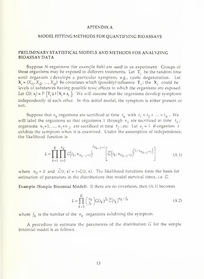
PRELIMINARY STATISTICAL MODELS AND METHODS FOR ANALYZINGBIOASSAY DATA

Suppose N organisms (for example fish) are used in an experiment. Groups of

these organisms may be exposed to different treatments. Let T- be the random time

until organism i develops a particular symptom, e.g., cystic degeneration. Let

Xj = (Xyp X^, .../ X- ) be covariates which (possibly) influence Tt

; the X- could be

levels of substances having possible toxic effects to which the organisms are exposed.

Let Git; xp = P [Tj- < t IX,- = x^ ]. We will assume that the organisms develop symptoms

independently of each other. In this initial model, the symptom is either present or

not.

Suppose that nkorganisms are sacrificed at time t

kwith r, < f

2< ••• < tv We

will label the organisms so that organisms 1 through nxare sacrificed at time f

T;

organisms fl-,+1, ..., n^ + n2

are sacrificed at time t2

; etc. Let s- = 1 if organism i

exhibits the symptom when it is examined. Under the assumption of independence,

the likelihood function is

K n kbnk_i+i

i-nffa'^-i*) "5('*-^-Hf"'"

M+ ')

jt=i 1=1

(A.l)

where w = ^ an<^ G(f; x) = 1-G(f; x). The likelihood functions form the basis for

estimation of parameters in the distributions that model survival times, i.e. G.

Example (Simple Binomial Model). If there are no covariates, then (A.l) becomes

L = fl{n

fk

k )G(tk )

fk G(tkr^ (A.2

k=\V J

where fk is the number of the nk

organisms exhibiting the symptom.

A procedure to estimate the parameters of the distribution G for the simple

binomial model is as follows.

13

MAXIMUM LIKELIHOOD ESTIMATION IN THE SIMPLE BINOMIAL MODEL

(a) Likelihood and Parameter Estimation Formulas

Assume the distribution of the time to appearance of a symptom, G, is a

function of the parameters , j = 1, ..., J. In this section we discuss maximumlikelihood estimation of for the simple binomial model. Presumably the n

k

subjects examined at time tk

, k = 1,2, ..., K have all been subjected to a commondosage of a potential toxin. The purpose of the present analysis is to predict survival

probabilities as they depend on such dosage. The log-likelihood function for the

simple binomial model is

Kf \

l=T^{nf"yfk^G(tk ;Q) + (nk -fk )\nG(tk ;Q) (A3)

where = (0^, ..., 0,Y Differentiating, we obtain

K

-1d9j ^G(tkl Q)de

j

3 GM) +b"^G(tk ;B) d6

G(t k ;Q)

= 1Kf

k \\-G(tk ;Q)]-(nk -fk )G(tk ;e)

k=\G(t k ;Q)G(tk ;Q)

\

d9i

G(tk ;d)

K

= 1k=1

fk-nkG[tk ;B)

'

G(t k ;B)G{tk ;Q) 30,G(tk ;Q). (A.4)

Since E[ik ]=n kG(tk ;Q)

dQjdem

k ^|-G(*jk;e)-|-G(f

fc;e)

Ide

nk

dem

*=1G{tk ;Q)G{tk ;B)

(A.5)

Thus a Newton procedure for finding the maximum likelihood estimates of

{#;/' = 1, ..., /} would iteratively solve the system of linear equations

J-ile°)+ x30m=\

ddjB6m{'«<) (A.6)

14

where 6 =(0|,...,0j . Such iterative procedures can be programmed for a digital

computer, and the resulting parameter values can be used to compute predictions for

survival probabilities, or risk, as the latter depend upon the parameters of such

models as described in Appendix B.

15

APPENDIX B. TWO-STAGE CLONAL-EXPANSION MODEL

In this appendix we present a birth-death model for the distribution of time

until a normal cell becomes promoted to a tumor.

We first develop an expression for the distribution of random time, S, until an

initiated cell or one of its descendants becomes malignant.

Assume that there is one initiated cell at time 0. Such cells divide at anexponential rate /3, and die at an exponential rate 8. Any initiated cell turns

malignant at an exponential ratefj.;

i.e. fi is the promotion rate.

(a) Time to Promotion of an Initiated Cell

Let S be the random time at which some initiated cell or its descendent turns

malignant; note that S may actually be infinite if the population of initiated cell andits descendents dies out. Put

z(t) = P{S>t}.

The following probability argument provides an equation for z(t): the event that

S > t+A (A > 0) occurs if (i) neither birth (cloning), death, or promotion occurs in

(0, A) and promotion does not occur in (A, t+A); the probability of this is

[1 - {fi+&+Li)A + o(A)]z(t); or (ii) birth/cloning occurs in (0,^) and no promotion occurs

in (A, t+A); the probability of this event is [@A + o(z\)]z 2 (0, where the square

recognizes that at time A there are now two independent clonal families to be

considered; or (iii) the original initiated cell dies in (0, A), the probability of which is

SA + o(A). Sum these three terms to obtain the probability that S > t+A:

z(t + A) = (M/3 +5 + li)A)z{t) + pAz2 (t) + SA.

Now subtract z(t) from each side, divide by A and let A —> 0. The result is the

differential equation

^ = -(p + 8 + ^)z(t) + Pz2(t) + S (B.l)

Hence z{t) satisfies a Riccati equation with initial condition

2(0) = 1 (B.2)

The solution to (B.l) with initial condition (B.2) is

16

if)_ PlO-P2)-P2(l-M^-^

I_p2 _(l_ pi)/(P1-P2)*

where p T 2are the solutions to the quadratic equation

f * 8 Px - 1 + - + —

I P Prh

(B.3)

(B.4)

Pl,2 =2

15 P

1 + — + —£ P

i5 P

1 + — + —P P) P

(B.5)

1/2

Since V+73+73/ _4B ^ \1 +73+ ft),

both pj and p2are positive. Further

p2 < 1 and

Pi " P2 = 15 P] A S

1 +— +— -4—P P) P

>0.

Hence,

lim z(f) = P2- (B.6)

If the death rate 5=0, then p = and lim PfT > t } = 0; if 8 = 0, then there is no deathz

t -»«,

of initiated cells and thus an initiated cell will transition to a malignant cell in a

finite time with probability 1. If <5> 0, then the initiating cells can die, thus

preventing a transition to malignancy and hence lim P{T> t} = p2>0.

t —> °°

(b) Model for the Time until a Normal Cell becomes Malignant (is Promoted to

Tumor)

Assume that each normal cell is initiated at an exponential rate Aq. Let N be the

total number of normal cells in an organ. Let T denote the first time a normal cell

transitions to a malignant cell.

17

-iN

P{T>t} = e~XOt +ix e~

XOSz{t-s)ds (B.7)

where 2 is a given in (B.3). Assume Aq is small and put X = XqN, a constant. Then

t

P{T > t} « exp NlnN £J

2(s)* (B.8)

= exp

t

. z(s)ds-Xt + X I (B.9)

= exp A(Pl -l)f-A-lnl_ p2+ (p 1

_ 1)/(Pl-P2V

P1-P2(B.10)

BIBLIOGRAPHY AND REFERENCES

Efron, B. and R. Tibshirani, "Bootstrap Methods for Standard Errors, ConfidenceIntervals, and other Measures of Statistical Accuracy," Statistical Science, Vol. 1,

(1986), pp. 54-77.

Gardner, H.S., van der Schalie, M.J. Wolfe and R.A. Finch (1990). "New methods for

on-site biological monitoring of effluent water quality." In Situ Evaluations of

Biological Hazards of Environmental Pollutants, ed. by S. S. Sandhu et al, PlenumPress, 1990; pp. 61-69.

Gaver, D. P. and P. A. Jacobs, Susceptibility and Exposure Variation in the Two-stage

Clonal Expansion Model, in progress.

Harris, C. C, "Interindividual Variation in Human Chemical Carcinogenesis:Implications for Risk Assessment," Scientific Issues in Quantitative Cancer Risk

Assessment (Abbreviate SIQCRA) ed. by S. H. Moolgavkar. Birkhauser. Boston,

1990. pp. 235-251.

Karlin, S., and H. M. Taylor, A Second Course in Stochastic Processes, AcademicPress, New York, 1981.

Kopp-Schneider, A., C. J. Portier and F. Rippman, "The Application of a Multistage

Model that Incorporates DNA Damage and Repair to the Analysis of

Initiation/Promotion Experiments," Math. Biosciences, Vol. 105, 1991, pp. 139-166.

18

McCullagh, P., and J. A. Nelder, Generalized Linear Models, Chapman and Hall,

New York, 1983.

Moolgavkar, S. H., and D. J. Venzon, "Two-event Models for Carcinogenesis:Incidence Curves for Childhood and Adult Tumors," Math. Biosciences, Vol. 47,

1979, pp. 55-77.

Moolgavkar, S. H., "Model for Human Carcinogenesis: Action of EnvironmentalAgents," Environmental Health Perspectives, Vol. 50, 1973, pp. 285-291.

Moolgavkar, S. H., N. E. Day and R. G. Stevens, "Two-stage Model for

Carcinogenesis: Epidemiology of Breast Cancer in Females," JNCl, Vol. 65, 1983, pp.559-569.

Portier, C. J., "Two-stage Models of Tumor Incidence for Historical Control Animalsin the National Toxicology Program's Carcinogenicity Experiment," /. of Toxicology

and Environmental Health, Vol. 27, 1989, pp. 21-45.'

Portier, C. J., "Utilizing Biologically Based Models to Estimate Carcinogenic Risk,"

SIQCRA, pp. 252-266.

Van Beneden, R. J., K. W. Henderson, D. G. Blair, T. S. Papas, and H. S. Gardner,

"Oncogenes in hematopoietic and hepatic fish neoplasms." Cancer Research (Suppl.),

Vol 50, pp. 5671s-5674s.

19

o

CO

ro

o o o X-

(Y.

LdZUJoLUQ(J <X)

^ <O M ro<X

CJ ozLJ

en

O 2<

X cr1- <L

Q_<o

CD

LJ 7LjJ I*)

h-<LUq:h-LULYQ_

oCD

I L

O 1

o ooo X-

o o o X-

o X-

X-

o X-

o X

J I L

80 90 ro

ayvzvH

10

jy

-X i

OO

OLO

IDc\J

O

LU

<->

Ml

20

O<CTUJZLU .

OLUn Q

C£

o <N7 <o X[£ OI (To

fc]^ :>IjJ <n a:

<T CL

CO

ro

O

QUJ\-

LU

Q_

to

to

CD

1

o

-2vy ooo o V o O O

*

—

>\

o o o X-

X- D

I I I 1 I

80 90 fr"0

aavzvH

soj L

oLO

LOf'J

OUJ(J

o\o

21

OlOQ_

OzoenXoin Q

ct:

<(/) M3 <

XCLO oh 1

LL

z tj

z 2LlI IT.

CJ <

CD X-

ro

X

OLU\-

Q_

Q_

o

CD

tn

CD

ro

cd

ro

O1

oo oX-

I

o X-

80 90

ayvzvH

frO 20

D<> MOO

o

in

o

O\-

o

o

V- v w

22

:iS,

eci hi ec e

DWI *> oh

\ i i i i i i i

on ot

PWM JO OH

J

1

if £gf 8-

.;

•

-

I

i i i i i i i «OB ot

crwmt jo onas DC: Kit

ITWWII iC OK

8-

2UJO 2_ O

IIP 2

-»- * ' ' ''

J

L3Icrw«* jooh

OUWIll JO OH

UJCl

Ll.1 u

rr h-

n f)>-

h- ( )

C2

n8"

r-C

5 8~

rJ

STW»« JO OK ET^"^ JP OX

1

ITkJKVS jo oh

I

3 8-

1 1 L 1 i

4_L _ 1 _J

- $

DVWI JC OH

2Ll)O 2xg

'-'

S|gg3 8*

C 2 « « » • * •LU uj trw*** jo ok

5 O

I i i !001 01 •

CTwmt jo oh

J:3 8"

£

Ct

ot ooi

crwmt jo oh

1

Ki ODi

trw>»>t jo oh

r—UJ urr >—

n to>

i— c >

o2

ESo i

23

_n

3

-

Si —4.

r^[

-

OR 002 0C1 001 Ot

ETMHVf JO OHOCI OOI Ot 001 R

STW»<W JO OH

PRETREATED WITH DEN° tce NEOPLASMS;CHRONIC POP ° ™juo n mo

8w n

O TCE3 MO

NO FISH HAVE NEOPLASMS

s

WAZAPO

25 TCE3 MO

h?

St

fl- J i i i i i_

0.4 OSHAZARO

OS 1.0

H _l I 1_

0.4 OSHAZAPO

25 TCES UO

8 1.0

'I'llI

04 OSHAZARD

OS 1.0

*82

Ik

PRETREATED WITH DEN5° tce NEOPLASMS,CHRONIC POP so tce3 MO 6 MO

NO FISH

HAVE NEOPLASMS

HAZARO

100 TCE3 UO

-k i i '

0.2 0.4 OSHAZARO

s

*8?

9 -

i t i i

0.8 1.0

_=_j I u0.4 0.8

MAZAPO

100 TCE

8 MO

8 1.0

0.4 0.8 0.8

HAZAPO

Figure 5

24

LUOLUQOI—CO>-ooLU

iS

oo

COLU

CL<\—CO\—OOm

>-° *—(j]—

*

z . • o x-gj_*$

Q_

oo

CLooK—Qj—

*

o X [3]—

X

o<

Q_UJft:

BOOTSTRAP

N

Y°*-(5}-*

ooin

>-a1*-g]-X)

! 1 11 1 1 1

oo

c

LUQ

21 8 fr

1S3 3WI1 NV3W 001

O

LOCM

O

LUo\—

o

o

01

25

PRETREATMENT WITH DEN

PERCENTTCE

I 3

LOG MEAN nue

325 'ERCENT

TCE

8 .

t/>

—

I

isis"

i

-

a

",, J" _J1 2

loc mean nue

50 PERCENTTCE

LOC ViEAN HUE

a.

100 PERCENTTCE

LOG MEAN TTWE

LOG MEAN TIME TO CYSTIC DEGENERATIONNO PRETREATMENT WITH DEN

PERCENTTCE

LOC *i£AN HUE

?

3-

23 PERCENTTCE

LLOC UEAN nuE

ii

8-

J

50 PERCENTTCE

On- J I I !_

S 12

LOC KIEAN TIME

8-

100 PERCENTTCE

LOC MEAN HUE

Figure 7

26

o

COLxJ

Ld v

OO

LdQ

UJ

<bJq:h-UJ

Q_

ro oUJ pC

CD °£

a: zz> oo zO II

o zoUJQ

UJQo

en ^>-O CL

m'ujO I!

CLUJ

L> J

otDX-

<D0 X-

<**-

UJ OCTT>X-

-X

-X O

o

encm

ox;

oo oo X-

LU

I

ooX-

J I L

-X°

J L

oLiJ

OI—

n1 (_ X 80^ Lj

90 fr

GOcJd 1S3

20

— v s. -

27

LdQX U.

I-ZLd

I—

Dlh-Ld01Q_

O

O

bJ ^

§5m °£

oo cl

3 oo zo II

o zoLlIu

°8>-O CL

h-00LJ

Ld

°°X1

o|[—X-

o«*<[Jj

Xo

o o«X-

Ld o «H-

Ld

o6<— N^

c

Ld

• •nrr.

OX-

-03-*"

3D-I

1 [_ X 90COLd

Ld

90 V'O

aodd 1S3

Z'O

oo

om

C\l

oLdo

• P*

28

D_OOl

O2^ , >

C ) oORE ETRIZ

O00 rv

z

M

OCCURS

L;N

=

N0NPA

LUQ

^ CO LJ

L- ^r ozLU

1—<

o ^

° .iLUrr en llJ

h- Q_LU

COG_ LU

LU oooX-

LU PV {rj.-

o <X-

LJ ocxt*-

o o X—"B"^

LjJ oX-a1

1

COLU t^

X 8

LJ

90 V'O

80yd 1S3

20

oo

oin

CxJ

oLJ(J

0J

29

r-^1

UJ \ I

o °1- \

I <p (r-\z Ul 1 1 1

1

. r?y* Z

f'J

IjJ

llk»M » OM

U5

or Va o

^1 I I-

g

* *8

'Lr^

1 t ill1

'I

I1WH JO OM

^

-J 1 I I I l_

zUJQ

I

n1.11-

IS

L.

Qt-oz

I ' 1 I I I-

IH>M JO OM IJkJM JO OM HW*t A OM nwi » on

SI

uj 1/1

^HUM JO OM

-J 1 1

l»UM jo on

"^

-J 1 1 • 1 i_

UUTM JO OM•» •

-I 1 1 I l_

•n*** JDOM• t

'30

llk*~> JO OH

7UJo z

siUJ"''O z "

UJ U

a °Lj ua £»- ooz

* * 1—1—1—_Ml KM f*

tlW** JO OM

"^-J I I I I I-

•J**** JO OM

'I

I7VWI JO OM

INITIAL DISTRIBUTION LIST

1. Library (Code 52) 2

Naval Postgraduate School

Monterey, CA 93943-5000

2 Defense Technical Information Center 2

Cameron Station

Alexandria, VA 22314

3. Office of Research Administration (Code 81) 1

Naval Postgraduate School

Monterey, CA 93943-5000

4. Prof. Peter Purdue 1

Code OR-PdNaval Postgraduate School

Monterey, CA 93943-5000

5. Department of Operations Research (Code 55) 1

Naval Postgraduate School

Monterey, CA 93943-5000

6. Prof. Donald Gaver, Code OR-Gv 5

Naval Postgraduate School

Monterey, CA 93943-5000

7. Prof. Patricia Jacobs 5

Code OR/JcNaval Postgraduate School

Monterey, CA 93943-5000

8. Center for Naval Analyses 1

4401 Ford AvenueAlexandria, VA 22302-0268

9. Dr. David Brillinger 1

Statistics DepartmentUniversity of California

Berkeley, CA 94720

10. Prof. W. R. Schucany

Dept. of Statistics

Southern Methodist University

Dallas, TX 75222

31

11. Prof. H.Solomon 1

Department of Statistics

Sequoia Hall

Stanford University

Stanford, CA 94305

12. Dr. Ed Wegman 1

George Mason University

Fairfax, VA 22030

13. Dr. NeilGerr 1

Office of Naval Research

Arlington, VA 22217

14. Dr. J. Abrahams, Code 1111, Room 607 1

Mathematical Sciences Division, Office of Naval Research

800 North Quincy Street

Arlington, VA 22217-5000

15. Prof. D. L. Iglehart 1

Dept. of Operations Research

Stanford University

Stanford, CA 94350

16. Prof. J. B. Kadane 1

Dept. of Statistics

Carnegie-Mellon University

Pittsburgh, PA 15213

17. Prof. J. Lehoczky 1

Department of Statistics

Carnegie-Mellon University

Pittsburgh, PA 15213

18. Prof. M. Mazumdar 1

Dept. of Industrial Engineering

University of Pittsburgh

Pittsburgh, PA 15235

19. Prof. Joseph R. Gani 1

Mathematics DepartmentUniversity of California

Santa Barbara, CA 93106

20. Prof. Frank Samaniego 1

Statistics DepartmentUniversity of California

Davis, CA 95616

32

21. Prof. Tom A. Louis

School of Public Health

University of Minnesota

Mayo Bldg. A460Minneapolis, MN 55455

22. Prof. Brad Carlin

School of Public Health

University of Minnesota

Mayo Bldg A460Minneapolis, MN 55455

23. Dr. John OravBiostatistics Department

Harvard School of Public Health

677 Huntington Ave.

Boston, MA 02115

24. Dr. D. C Hoaglin

Department of Statistics

Harvard University

1 Oxford Street

Cambridge, MA 02138

25. Prof. Carl N. Morris

Statistics DepartmentHarvard University

1 Oxford St.

Cambridge, MA 02138

26. Dr. John E. Rolph

RAND Corporation

1700 Main St.

Santa Monica, CA 90406

27. Prof. J. W. TukeyStatistics Dept., Fine Hall

Princeton University

Princeton, NJ 08540

28. Dr. D. Pregibon

AT&T Bell Telephone Laboratories

Mountain AvenueMurray Hill, NJ 07974

33

29. Dr. Jon Kettenring

Bellcore

445 South Street

Morris Township, NJ 07962-1910

30. Dr. D. F. Daley

Statistic Dept. (LA.S.)

Australian National University

Canberra, A.C.T. 2606

AUSTRALIA

31. Koh Peng KongOA Branch, DSOMinistry of Defense

Blk 29 Middlesex RoadSINGAPORE 1024

32. Professor Sir David CoxNuffield College

Oxford, OXI INFENGLAND

33. Dr. A. J. LawrenceDept. of Mathematics,

University of BirminghamP. O. Box 363

Birmingham B15 2TTENGLAND

34. Dr. D. Vere-Jones

Dept. of Math, Victoria Univ. of Wellington

P. O. Box 196

Wellington

NEW ZEALAND

35. Dr. Robert Carpenter

Naval Medical Research Institute, Toxicology Unit

Wright-Patterson Air Force Base,

Dayton, OH 45433

34

DUDLEY KNOX LIBRARY

3 2768