NAVAL POSTGRADUATE SCHOOL · 12b. DISTRIBUTION CODE 13. ABSTRACT (maximum 200 words) This study incorporated two approaches to determine the thermal conductivity of nanocomposite

NAVAL

POSTGRADUATE SCHOOL

MONTEREY, CALIFORNIA

THESIS

Approved for public release; distribution is unlimited

FINITE ELEMENT AND MOLECULAR DYNAMICS MODELING AND SIMULATION OF THERMAL

PROPERTIES OF NANOCOMPOSITES

by

Daniel C. Kidd

June 2007

Thesis Advisor: Young Kwon

THIS PAGE INTENTIONALLY LEFT BLANK

i

REPORT DOCUMENTATION PAGE Form Approved OMB No. 0704-0188 Public reporting burden for this collection of information is estimated to average 1 hour per response, including the time for reviewing instruction, searching existing data sources, gathering and maintaining the data needed, and completing and reviewing the collection of information. Send comments regarding this burden estimate or any other aspect of this collection of information, including suggestions for reducing this burden, to Washington headquarters Services, Directorate for Information Operations and Reports, 1215 Jefferson Davis Highway, Suite 1204, Arlington, VA 22202-4302, and to the Office of Management and Budget, Paperwork Reduction Project (0704-0188) Washington DC 20503. 1. AGENCY USE ONLY (Leave blank)

2. REPORT DATE June 2007

3. REPORT TYPE AND DATES COVERED Master’s Thesis

4. TITLE AND SUBTITLE Finite Element and Molecular Dynamics Modeling and Simulation of Thermal Properties of Nanocomposites 6. AUTHOR(S) Daniel C. Kidd

5. FUNDING NUMBERS

7. PERFORMING ORGANIZATION NAME(S) AND ADDRESS(ES) Naval Postgraduate School Monterey, CA 93943-5000

8. PERFORMING ORGANIZATION REPORT NUMBER

9. SPONSORING /MONITORING AGENCY NAME(S) AND ADDRESS(ES) N/A

10. SPONSORING/MONITORING AGENCY REPORT NUMBER

11. SUPPLEMENTARY NOTES The views expressed in this thesis are those of the author and do not reflect the official policy or position of the Department of Defense or the U.S. Government. 12a. DISTRIBUTION / AVAILABILITY STATEMENT Approved for public release; distribution is unlimited

12b. DISTRIBUTION CODE

13. ABSTRACT (maximum 200 words) This study incorporated two approaches to determine the thermal conductivity of nanocomposite material

using numerical modeling and simulation. The first was to look at the nanocomposite material at the macro level using a continuum model. The second approach broke the problem down to the atomic level and addressed the inter-atomic reactions using the Molecular Dynamics model.

The continuum model was used to determine the optimal placement and alignment of the nanoparticles within a nanocomposite, to provide the largest enhancement of thermal conductivity for the composite. During this process the effects of the particle size and spacing were investigated to determine the function that interparticle spacing and particle size plays in the thermal conductivity of the composite.

The Molecular Dynamics model was also used to calculate the thermal conductivity of nanocomposites given the thermal conductivity of the nanoparticles and the base material.

15. NUMBER OF PAGES

69

14. SUBJECT TERMS: Finite Element Method; Molecular Dynamics; Nanocomposites; Thermal Conductivity; Carbon Nanotubes, Nanoparticles

16. PRICE CODE

17. SECURITY CLASSIFICATION OF REPORT

Unclassified

18. SECURITY CLASSIFICATION OF THIS PAGE

Unclassified

19. SECURITY CLASSIFICATION OF ABSTRACT

Unclassified

20. LIMITATION OF ABSTRACT

UL NSN 7540-01-280-5500 Standard Form 298 (Rev. 2-89) Prescribed by ANSI Std. 239-18

ii


iii

Approved for public release; distribution is unlimited

FINITE ELEMENT AND MOLECULAR DYNAMICS MODELING AND SIMULATION OF THERMAL PROPERTIES OF NANOCOMPOSITES

Daniel C. Kidd Lieutenant, United States Navy

B.S., The United States Naval Academy, 1998

Submitted in partial fulfillment of the requirements for the degree of

MASTER OF SCIENCE IN MECHANICAL ENGINEERING

from the

NAVAL POSTGRADUATE SCHOOL June 2007

Author: Daniel C. Kidd

Approved by: Young Kwon, PhD. Thesis Advisor

Anthony Healey Chairman, Department of Mechanical and Aeronautical Engineering

iv


v

ABSTRACT

This study incorporated two approaches to determine the thermal

conductivity of nanocomposite material using numerical modeling and simulation.

The first was to look at the nanocomposite material at the macro level using a

continuum model. The second approach broke the problem down to the atomic

level and addressed the inter-atomic reactions using the Molecular Dynamics

model.

The continuum model was used to determine the optimal placement and

alignment of the nanoparticles within a nanocomposite, to provide the largest

enhancement of thermal conductivity for the composite. During this process the

effects of the particle size and spacing were investigated to determine the

function that interparticle spacing and particle size plays in the thermal

conductivity of the composite.

The Molecular Dynamics model was also shown to calculate the thermal

conductivity of nanocomposites given the thermal conductivity of the

nanoparticles and the base material.

vi


vii

TABLE OF CONTENTS

I. INTRODUCTION............................................................................................. 1 A. JUSTIFICATION .................................................................................. 1 B. OBJECTIVES....................................................................................... 3

II. BACKGROUND AND THEORY ..................................................................... 5 A. THE CARBON NANOTUBE AND NANOCOMPOSITES .................... 5

1. Carbon Nanotubes................................................................... 5 2. Nanocomposites...................................................................... 7

B. THE CONTINUUM METHOD (FINITE ELEMENT METHOD)............ 10 C. MOLECULAR DYNAMICS ................................................................ 11

1. Classical Molecular Dynamics Method................................ 11 2. Newton-Hamiltonian Dynamics for the Classical

Molecular Dynamics Simulation........................................... 12 3. Molecular Dynamics Soft Sphere (MDSS) ........................... 13

D. CONDUCTION ................................................................................... 15

III. MODELING................................................................................................... 19 A. CONTINUUM METHOD..................................................................... 19

1. Pre-processing....................................................................... 19 a. Settings and Boundary Conditions in ANSYS.......... 19 b. Meshing ....................................................................... 20

2. Processing and Post-processing ......................................... 21 B. MOLECULAR DYNAMICS ................................................................ 21

IV. RESULTS AND DISCUSSION ..................................................................... 25 A. CONTINUUM METHOD..................................................................... 25

1. Low Volume Fraction Models ............................................... 25 2. Ten Percent Volume Fraction ............................................... 25

a. Eight Particles ............................................................. 25 b. Rectangular Strips ...................................................... 29 c. Ten Percent Discussion ............................................. 31

3. The 4.7 Percent Volume Fraction Models............................ 31 a. Particle Size Comparisons ......................................... 32 b. Particle Spacing Comparison .................................... 39

B. MOLECULAR DYNAMICS RESULTS............................................... 42

V. CONCLUSIONS............................................................................................ 45 A. CONTINUUM MODEL........................................................................ 45 B FUTURE WORK WITH THE CONTINUUM MODEL.......................... 47 C. MOLECULAR DYNAMICS CONCLUSION ....................................... 47 D. MOLECULAR DYNAMICS FUTURE WORK..................................... 48

LIST OF REFERENCES.......................................................................................... 51

INITIAL DISTRIBUTION LIST ................................................................................. 53

viii


ix

LIST OF FIGURES

Figure 1. (a) A schematic diagram showing how a hexagonal sheet of graphite is ‘rolled’ to form a CNT. (b) Illustrations of the two nanotube structures the Armchair and Zig-Zag from (a). [6]................. 6

Figure 2. Thermal conductivity of SWNTs as a function of temperature. The inset highlights low temp behavior, the solid line is a linear fit for data below 25K. [8]............................................................................... 7

Figure 3. Solid dots represent the experimental results of the normalized conductivity data ke/kf (ke is κ of the composite, kf is κ of the fluid) CNT in oil suspension, compared to the dotted lines representing theoretical models for the enhancement of thermal conductivity in composite. κ ratio is 13800. [11] ........................................................ 8

Figure 4. Solid Lines represent the thermal conduction enhancement using equation (2) compared to the experimental results (the solid dots) from reference. [14] ............................................................................ 10

Figure 5. FCC structure of the primary material with two groups of atoms of a secondary material imbedded in the solid. The secondary material atoms are the red asterisk. ................................................................. 23

Figure 6. FCC structure of the primary material with a continuous section of secondary material the entire x-dimension of the structure. The atoms of the secondary material are indicated by the red asterisk. .... 24

Figure 7. Eight particles (evenly spaced) diameter 0.6308, a 10% volume fraction. Dimensions of the plate are 5 in the x-direction 5 in the y-direction.............................................................................................. 27

Figure 8. Heat Flux in the x-direction. Plate with eight particles evenly spaced, diameter 0.6308 a 10% volume fraction. The superimposed graph shows the nodal values of the heat flux as it varies on the boundary. ...................................................................... 27

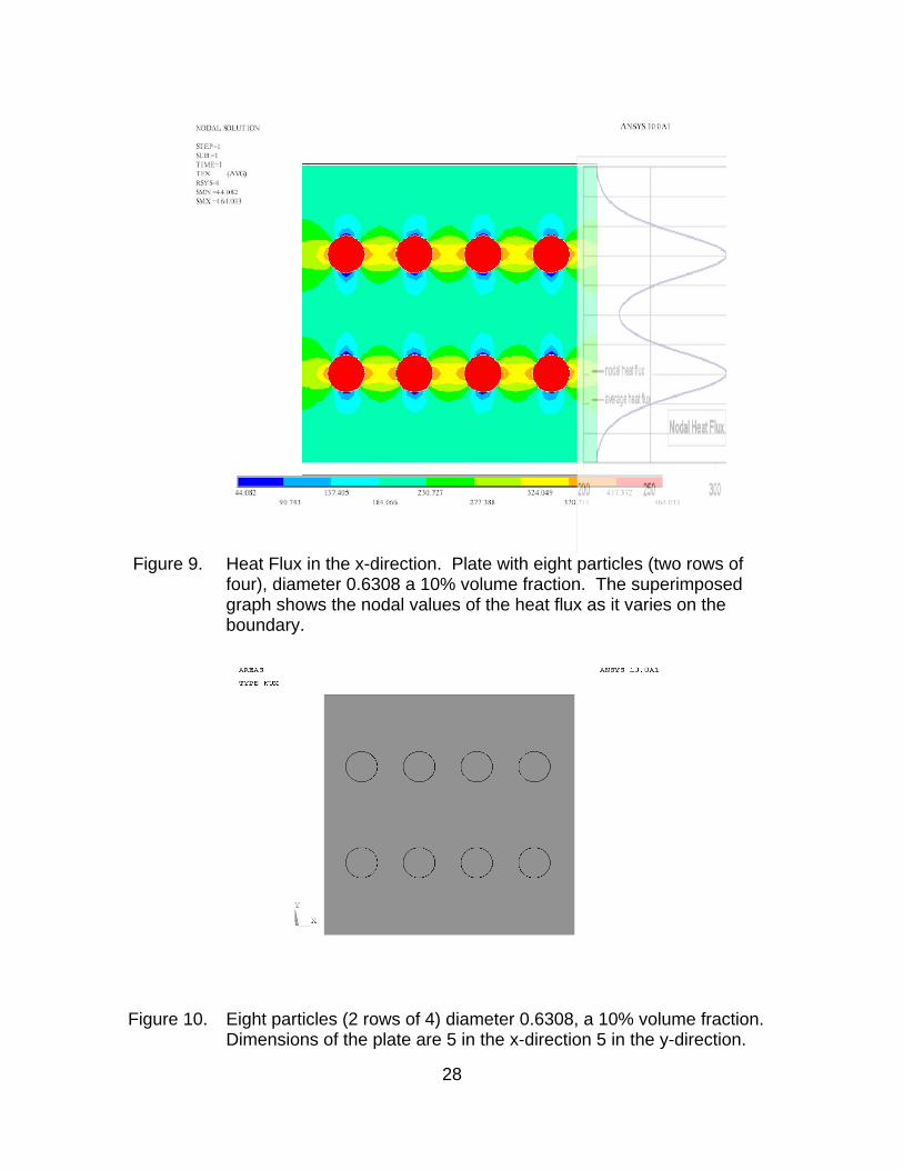
Figure 9. Heat Flux in the x-direction. Plate with eight particles (two rows of four), diameter 0.6308 a 10% volume fraction. The superimposed graph shows the nodal values of the heat flux as it varies on the boundary. ........................................................................................... 28

Figure 10. Eight particles (2 rows of 4) diameter 0.6308, a 10% volume fraction. Dimensions of the plate are 5 in the x-direction 5 in the y-direction.............................................................................................. 28

Figure 11. The *effκ of a plate with 10% volume fraction of a secondary

material incorporating Eight particles of diameter 0.6308................... 29 Figure 12. The *

effκ of a plate with a constant 10% volume fraction, in all three cases, of a secondary material in rectangular strips........................... 30

Figure 13. The *effκ of a plate with a constant 10% volume fraction, in all three

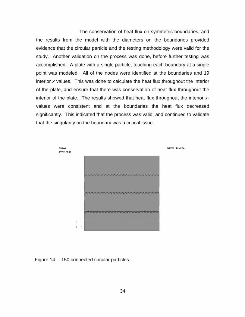
cases, of a secondary material in rectangular strips κ ratio=10,000. 30 Figure 14. 150 connected circular particles. ........................................................ 34

x

Figure 15. The *effκ of a plate with 4.7% volume fraction of a secondary

material; particles of varying number and diameter; circular particles with points of singularity at the boundaries. Shows that there is an upper limit to the *

effκ which is inconsistent with the earlier models using the rectangular strips. ........................................ 35

Figure 16. 7 connected circular particles with half particles at the boundaries. ... 36 Figure 17. The *

effκ of a plate with 4.7% volume fraction of the secondary material; particles of varying number and size; circle diameter on the boundaries. Does not show any noticeable variation with the change of the particle size. Inconsistent with the rectangular strip models................................................................................................ 37

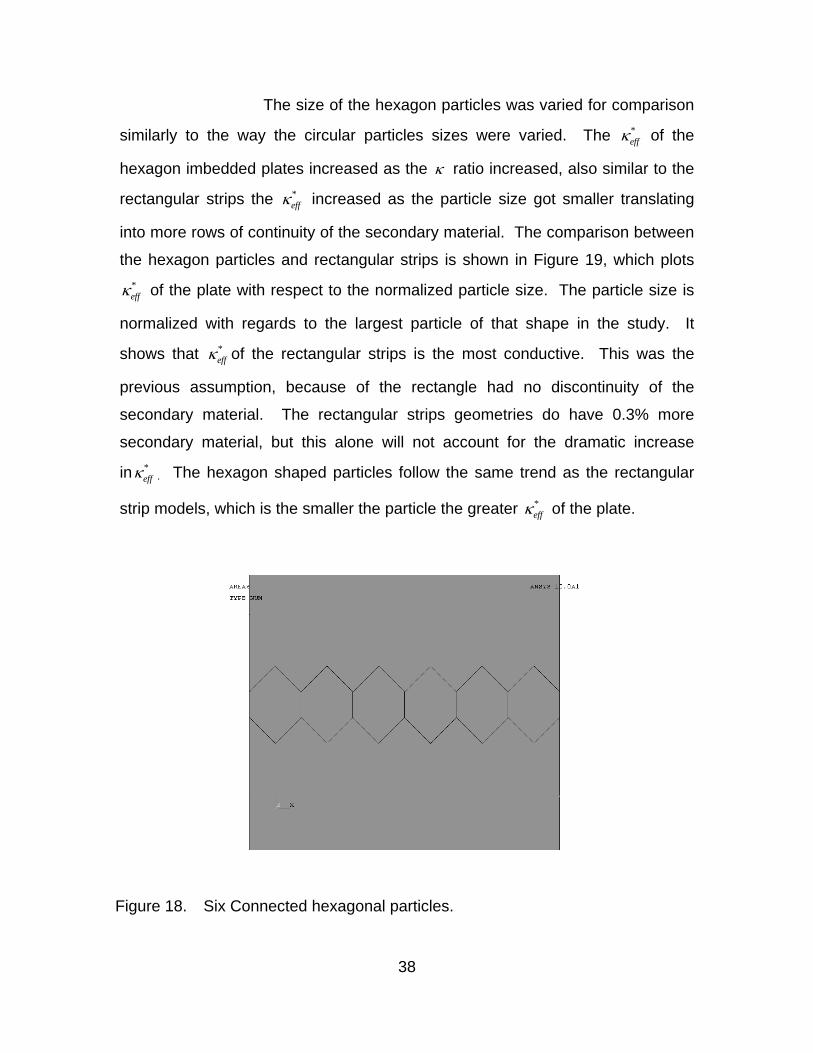
Figure 18. Six Connected hexagonal particles. ................................................... 38 Figure 19. Comparison between particle shapes: rectangle, hexagon and both

geometries are at an approximate volume fraction of 4.7%. κ ratio=10,000. ...................................................................................... 39

Figure 20. The *effκ of a plate as the spacing between particles is increased. ..... 41

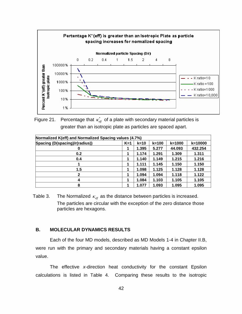
Figure 21. Percentage that *effκ of a plate with secondary material particles is

greater than an isotropic plate as particles are spaced apart. ............ 42 Figure 22. The effκ of the MD Models with the Constant Epsilon Materials......... 43 Figure 23. Normalized effκ of the Nanocomposite MD Models which have

Constant Epsilon Valued Materials as the Primary and Secondary Material............................................................................................... 44

xi

LIST OF TABLES

Table 1. The Heat Conductivity of the primary and secondary materials used in the MD models and the associated Sigma values. ......................... 24

Table 2. The *effκ of a plate with a constant 10% volume fraction, in all three

cases, of a secondary material in rectangular strips........................... 31 Table 3. The Normalized effκ as the distance between particles is increased.

The particles are circular with the exception of the zero distance those particles are hexagons.............................................................. 42

Table 4. Heat conductivity of the MD Models with the Constant Epsilon Value=1. ............................................................................................. 43

xii


xiii

ACKNOWLEDGMENTS

I would like to thank my thesis advisor Young Kwon for his guidance

throughout this learning experience. Every meeting we had, invigorated me and

motivated my excitement and interested in finding the answers and more of the

questions. I would also like to thank my parents, Craig and Elizabeth Kidd, who I

do not thank often enough for their guidance and sacrifices that supported me

throughout my early years; and their continued support even now that I am older.

Lastly I would like to thank my wife, Kimberly, without her love, support, and

dedication to me and our children, this thesis and degree would never be

possible.

xiv


1

I. INTRODUCTION

A. JUSTIFICATION

The world of technology is becoming smaller and more powerful.

Everywhere the hardware components are mimicking that trend; they are able to

process more information at faster speeds. There is, however, a price to be paid

to achieve the goal of the high power dense hardware components. The price is

heat. The power used to process and operate cause the byproduct heat.

Increasing temperatures in the components, without a means to dissipate this

heat, will initially cause degradation and quickly lead to failure of the components

and system.

The two modes of heat transfer that are typically used for cooling

hardware are conduction and convection. Conduction is involved by transferring

heat from the point of heat generation, within the component, to the housing or

external part of the component. Convection (either forced or free) then transfers

the heat from the outside of the component to a heat sink. A component that is

more power dense does not have as much material and cooling area than that of

a less power dense component. Less surface area may therefore reduce the

efficiency of heat transfer. The overall effect is that the component will not cool

sufficiently, then overheat, and ultimately fail.

The demand for more power dense hardware, therefore, will not be a

viable reality without viable cooling techniques. There are different possible

ways to address the cooling problem. The most general ways are to increase the

cooling potential of either the conduction, or the convection modes. This thesis

focuses on a method of using nanoparticles embedded into a base material to

create a more thermally conductive nanocomposite material. This material will

allow for greater heat dissipation from the point of generation to the convection

interface.

2

The assumption, that nanoparticles such as Carbon Nanotubes (CNT) are

much more conductive than the base material, leads to the hypothesis that the

addition of a small amount of nanoparticles into the base material will have a

great additive effect on the thermal conductivity of the entire composite material,

thus increasing the heat flux through the material.

Similar assertions have been made and demonstrated using CNT to

improve the strength and stiffness of composite materials. With as little as a one

percent (by weight) of CNT dispersed into a composite material the stiffness

increases between 36 and 42%; with a 25% increase in tensile strength. [1] It is

reasonable to think that similar advances could be made to composite materials

utilizing the thermal properties of the CNT.

Computer modeling and simulation will be used to numerically test this

idea and to calculate quantitative results of thermal conductivity of the material.

Previous experimental and theoretical work has been done to determine the true

potential of nanocomposites’ thermal properties. The studies have had mixed

results. Past experimental results have been considerably higher than some

older theories would have predicted. Analytic models have recently been offered

to explain the conductivity of the CNT and how they react within a composite.

These analytic models predict that the thermal conductivity of the composites can

be much higher than the experimental data has shown.

The experimental work may be hampered by the delicacy of the CNT.

Although they are very strong, because of their size they tend to intertwine with

other tubes. It is also difficult to disperse, align, and orient the CNT throughout

the composite to optimize their properties. Through computer modeling and

simulation the alignment issues are eliminated; placement of the nanotubes can

be specified throughout the composite, the spacing and orientation within the

composite can be dictated to accurately determine how those variations will

affect the thermal properties of the material. Models and simulations have limits

3

as well. The aim is to create and implement models that accurately mimic the

conditions in a real system and are able to provide reasonable results with

respect to the given loads.

B. OBJECTIVES

There are two goals of this thesis. First using numerical modeling and

simulation to determine the optimal placement and alignment of the nanoparticles

within a nanocomposite will be determined to provide the largest enhancement of

thermal conductivity for the composite. During this process, the effects of the

particle size and spacing will be investigated to determine the function that

interparticle spacing and particle size plays in the thermal conductivity of the

composite. Secondly a numerical model will be developed that will accurately

calculate the thermal conductivity of nanocomposites given the thermal

conductivity of the nanoparticles, and the base material and the volume fraction

of the nanoparticles in the composite. Two independent models will be

produced; a continuum model and a molecular dynamics model, to accomplish

the first and second goals, respectively.

4


5

II. BACKGROUND AND THEORY

This chapter will offer an overview of key components of the thesis. The

first section will discuss nanoparticles, such as Carbon Nanotubes, and

nanocomposites; whose properties are the primary, interest in this study. The

theory of conduction, the heat transfer mode of interest, will be discussed in the

second section. The other items covered in this chapter are the Continuum

numerical method incorporating the Finite Element Method and lastly Molecular

Dynamics. The continuum method and molecular dynamics are the basis for the

models that are used to simulate the heat transfer through the nanocomposites.

A. THE CARBON NANOTUBE AND NANOCOMPOSITES

1. Carbon Nanotubes

The Carbon Nanotube (CNT) has been widely studied since the discovery

in 1991. [2] The material properties are believed to be amazing; yield strength

greater than that of high strength steels; thermal conductivity comparable that of

diamonds (the most thermally conductive material known) [3]; excellent electrical

conductivity. With those properties, the possible uses of the CNT seem to be

unlimited, and new potential uses continue to propagate.

The Nanotube, as discovered by Iijima, is a seamless cylinder of graphite

layers. Further work with the CNT has shown that the cylinders can be formed

with fullerenes of carbon atoms capping the ends. The carbon atoms form a

benzene-type hexagonal lattice to form the shell of the tube. They arrange in

helical fashion around the tube’s long axis of the tubes. [2] The tubes are

approximately 2-10 nm in diameter (approximately 1/10,000 the diameter of a

human hair) and have been grown as individual Single Walled Nanotube to four

centimeters in length. [4]

6

Carbon based materials, in-plane pyrolytic graphite and diamonds, have

the greatest measured thermal conductivity of any material at moderate

temperatures. [5] The graphite cylinder that makes up the CNT have the same

hexagonal molecular structure as that of the in-plane graphite sheets, Figure 1

illustrates this.

(a) (b)

Figure 1. (a) A schematic diagram showing how a hexagonal sheet of graphite is ‘rolled’ to form a CNT. (b) Illustrations of the two nanotube structures the Armchair and Zig-Zag from (a). [6]

Although the nanotubes are two dimensional, the extremely small

diameter of the tubes reduces the dimensionality of the tube to practically one

dimension. This graphite molecular structure and the small diameter suggest

that CNT will have a thermal conductivity equivalent to that of diamonds. [7] The

carbon make up of the nanotubes and the small size facilitate the phonon-

phonon interaction in the axial direction of the CNT. The phonon-phonon

interaction is a major factor in the heat conductivity of a material; this will be

discussed further in the Conduction section of this report. Higher temperatures

increase the phonon-phonon reaction, which is illustrated in Figure 2, as the

thermal conductivity is a function of the temperature.

7

Figure 2. Thermal conductivity of SWNTs as a function of temperature. The

inset highlights low temp behavior, the solid line is a linear fit for data below 25K. [8]

The CNT have been studied extensively, experimentally and numerically

using Molecular Dynamics (MD). The results are almost as numerous as the

studies. One MD study reported the thermal conductivity (κ ) of a Single Walled

Nanotube (SWNT) to be 2980 W/m-K. [9] A second MD study of an identical

SWNT determined that κ = 6600 W/m-K (greater than that of a diamond). [10]

Still other studies of using experimental approaches have estimated κ to range

from 1750 to 5780 W/m-K for the SWNT. [8] Although there is a large range in

the results for the thermal conductivity, there is a commonality that the results

indicate that the CNT do have a high κ . The high thermal conductivity along

with the other material properties ensures that there will be continued interest in

developing CNT far into the future.

2. Nanocomposites

The nanocomposites are composite materials that typically have

nanoparticles imbedded into their matrix; these particles are typically CNT but

may be other nano-sized particles (for this report, the nanoparticles will be

assumed in general). The initial focus on the work of nanocomposites was the

hope of increasing material strength, which proved successful. More recently

8

there has been interest in the thermal advantages of nanocomposites. Most of

the work has focused on the experimental results trying to measure the thermal

conductivity of materials or creating analytical models that will accurately predict

the composites’ thermal conductivity. The results of these studies indicate that

the maximum potential for the thermal conductivity of nanocomposites has not

yet been achieved.

A 2001 experiment studied the thermal conductivity of oil with CNT in

suspension. The results showed that with a 1.0 vol% of CNT in suspension a

1600% enhancement of the thermal conductivity was recorded. Previous

theories of the conduction of fluids with particles in suspension predicted only a

10% increase in the conductivity. [11] The results of the 2001 study are shown

below in Figure 3.

Figure 3. Solid dots represent the experimental results of the normalized

conductivity data ke/kf (ke is κ of the composite, kf is κ of the fluid) CNT in oil suspension, compared to the dotted lines representing theoretical models for the enhancement of thermal conductivity in composite. κ ratio is 13800. [11]

The experimental results of solid nanocomposites in 2002 produced

results of 125% thermal conductive enhancement through an epoxy composite

9

with 1 wt% CNT. This increase translated into 0.5κ ≅ W/m K; which was

significantly lower than the researchers hoped to get according to the ”law of

mixtures” prediction of 10W/m K. [12]

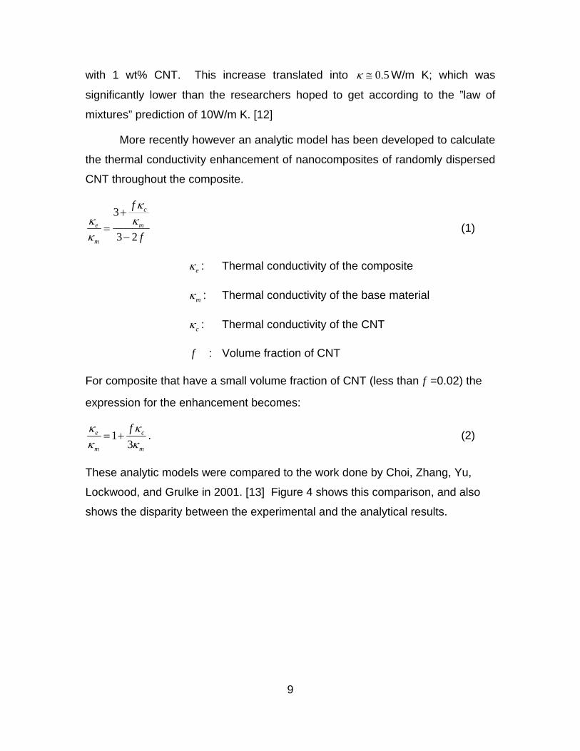
More recently however an analytic model has been developed to calculate

the thermal conductivity enhancement of nanocomposites of randomly dispersed

CNT throughout the composite.

3

3 2

c

e m

m

f

f

κκ κκ

+=

− (1)

eκ : Thermal conductivity of the composite

mκ : Thermal conductivity of the base material

cκ : Thermal conductivity of the CNT

f : Volume fraction of CNT

For composite that have a small volume fraction of CNT (less than f =0.02) the

expression for the enhancement becomes:

13

e c

m m

fκ κκ κ

= + . (2)

These analytic models were compared to the work done by Choi, Zhang, Yu,

Lockwood, and Grulke in 2001. [13] Figure 4 shows this comparison, and also

shows the disparity between the experimental and the analytical results.

10

Figure 4. Solid Lines represent the thermal conduction enhancement using

equation (2) compared to the experimental results (the solid dots) from reference. [14]

B. THE CONTINUUM METHOD (FINITE ELEMENT METHOD)

The Finite Element Method (FEM) is a numerical technique used to

calculate and solve problems that do not have an analytical solution or that the

system of interest is so complex that the analytic solution is too unwieldy to be

used as a practical tool in solving the problem. An analytic solution provides the

solution at an infinite number of points within the system; however, the FEM

produces a solution at only a finite number of locations. Increasing number of

location, referred to as nodes, in the system creates results that more closely

match the analytic solution. The cost of this accuracy is the computing time

associated with the calculations at each node.

The basis of the technique is to break the system up into a finite number

of elements and then implement the boundary conditions and material properties

for the system. The individual elements are modeled as homogeneous

members. Therefore the solution across the well defined element is relatively

easy to calculate.

The continuum computational process has been used in recent studies of

carbon nanotube based composites. [15] Most of the work using the continuum

11

method and carbon nanotube based composites has been focused on the

mechanical properties of the composites. It can, however, be assumed that

these same techniques can be implemented to study the thermal properties of

these emerging materials.

C. MOLECULAR DYNAMICS

The molecular dynamics approach is a simple one to grasp. It is, however,

very challenging to implement. The premise is that the location of every body in

a system is known at an initial time and the force on every body is also known.

Then every future location, velocity, acceleration force and energy can be

determined. The key is motion. The motion of molecules, regardless of whether

they are solid, liquid, or gas molecules, is the important critical characteristic to

determine all of the other values. The challenge of implementation is

determining the exact initial conditions. The bodies in the system at the

molecular level are enormous (there 6.022 x 1023 atoms per mole) and the time

step size is incredibly small (the order of 10-15 seconds) to accurately calculate

the atomic motion. These two parameters combine for an astronomical amount

of computing power and time.

1. Classical Molecular Dynamics Method

The classical MD method is to calculate the position and velocities of all of

the atoms as a function of time. The MD processor and solver are not concerned

with the physical state (solid, liquid, gas) of the particular atom. The atoms are

assigned an energy value, and it is this energy value that is the basis for the

motion of the particle. At the atomic level, the atoms vibrate and move

regardless of whether they are solid or fluid in nature. They will move more or

less depending on the energy state of the atom. That being the case, it is a

useful tool for modeling and simulating systems that containing multi-state and

multi material systems. There are no issues or difficulties with modeling and

analyzing of the interfaces between different states or materials, because the

analysis is done at the atomic level. Using the atoms energy, Newton’s second

12

law, Hamiltonian equation, and a potential energy function; the position and

velocities of the atoms are calculated for a time step. The calculations are

repeated for multiple time steps to calculate the solution.

The Quantum Molecular Dynamics model is another approach to the MD

solution process. It is a model which is considered beneficial if the simulation

and analysis is aimed at electron interaction between the atoms. The quantum

MD model and simulation tend to be much more complex and more time

consuming than that of the classical method, and as this work is not concerned

with the electron interaction among the atoms the Classical MD approach was

determined to be the correct choice. [16]

2. Newton-Hamiltonian Dynamics for the Classical Molecular Dynamics Simulation

When using the Newton-Hamiltonian Dynamics for MD simulation; the

motion of the atom (i) is caused by force (Fi) exerted by an intermolecular

potential energy (U). The motion of the atoms and applied forces are related

through Newton’s second law.

i iF mr= && (3)

Here m is the mass of the atom, independent of time and position.

Acceleration ( ir&&) is represented by the equation:

2

2i

id rrdt

=&& (4)

where ri is the vector that gives the atom’s position with respect to the coordinate

system’s origin. For a given N-atom system, Newton’s second law represents 3N

second order ordinary differential equation.

A conserved quantity in isolated systems is the total energy (E). It is

possible to identify the total energy as the Hamiltonian (H). H takes the form of

Equation (5); where p is the momentum of an atom and the potential energy U

results from the interaction between atoms.

13

21( , ) ( )2

N N Ni

iH r P p U r E

m= + =∑ (5)

Taking the derivative of Equation (5) with respect to the distance r, the explicit

relationship between the Hamiltonian and the potential energy is

i i

H Ur r

∂ ∂=

∂ ∂. (6)

The resultant Hamilton’s equations of motion are

ii

i

pH rp m∂

= =∂

& (7)

i ii

H p mrr

∂= − = −

∂&& . (8)

Using Equation (6) in the Equation (8) and comparing to Newton’s Law (3)

produces the equation.

ii i

H UFr r

∂ ∂= − = −

∂ ∂. (9)

Any conservative force can be written as the negative gradient of some potential

energy function U, and the forces from all of the other atoms determine the

acceleration of each atom in the given system. [17]

3. Molecular Dynamics Soft Sphere (MDSS)

The most important aspects of a classical MD code are the applied

potential energy functions and the finite difference method that is used. There

are two main categories for the pair potential energy functions as they relate to

the classic MD codes. They are the soft sphere potential and the hard sphere;

the soft sphere potential represents the continuous energy function with respect

to the inter-atomic distance, while the hard sphere potential represent a

discontinuous energy function. The soft sphere approach is used for this thesis.

MDSS simulations codes tend to use a Verlet type algorithm or Predictor-

corrector algorithm as the finite difference method to numerically solve the

14

differential equations of motion. These algorithms are usually chosen over the

Euler or the Euler-Cromer based algorithms, because the Euler and Euler-

Cromer tend to have numerical errors that are too big to tolerate at the small

scales that MD operates at. [16]

The MDSS code used for this thesis was originally developed by J.M.

Haile. [17] His code incorporates the Lennard Jones Potential (Equation (10)),

as the potential energy function, and uses Gear’s Predictor-Corrector Algorithm

to calculate the motion of the atoms.

12 6( ) 4 [( ) ( ) ]u rr rσ σε= − (10)

Gear’s Predictor-Corrector Algorithm:

Prediction: A fifth order Taylor series to describe the atoms position at t t+ Δ

based on the position and the derivatives at time t.

2 3 4 5( ) ( ) ( ) ( )( ) ( ) ( ) ( ) ( ) ( )2! 3! 4! 5!

iv vi i i i i i i

t t t tr t t r t r t r t r t r t r tΔ Δ Δ Δ+ Δ = + Δ + + + +& && &&& (11)

2 3 4( ) ( ) ( )( ) ( ) ( ) ( ) ( )2! 3! 4!

iv vi i i i i

t t tr t t r t r t r t r t r tΔ Δ Δ+ Δ = + Δ + + +& & && &&& (12)

2 3( ) ( )( ) ( ) ( ) ( )2! 3!

iv vi i i i i i

t tr t t r t r t r t r tΔ Δ+ Δ = + Δ + +&& && &&& (13)

2( )( ) ( ) ( )2!

iv vi i i i i

tr t t r t r t r t Δ+ Δ = + Δ +&&& &&& (14)

( ) ( )iv iv vi i ir t t r t r t+ Δ = + Δ (15)

( ) ( )v vi ir t t r t+ Δ = (16)

Evaluation: Intermolecular Force on each atom is calculated at t t+ Δ .

^( )iji ij

j i ij

u rF r

r≠

∂= −

∂∑ (17)

15

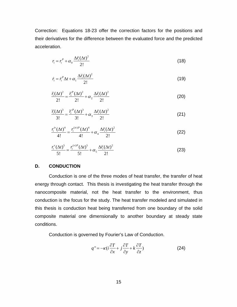
Correction: Equations 18-23 offer the correction factors for the positions and

their derivatives for the difference between the evaluated force and the predicted

acceleration.

2

0( )2!

P ii i

r tr r α Δ Δ= +

&& (18)

2

1( )2!

P ii i

r tr r t α Δ Δ= Δ +

&&& & (19)

2 2 2

2( ) ( ) ( )2! 2! 2!

Pi i ir t r t r tαΔ Δ Δ Δ

= +&& && &&

(20)

3 3 2

3( ) ( ) ( )3! 3! 2!

Pi i ir t r t r tαΔ Δ Δ Δ

= +&&& &&& &&

(21)

4 ( ) 4 2

4( ) ( ) ( )4! 4! 2!

iv iv Pi i ir t r t r tαΔ Δ Δ Δ

= +&&

(22)

5 ( ) 5 2

5( ) ( ) ( )5! 5! 2!

v v Pi i ir t r t r tαΔ Δ Δ Δ

= +&&

(23)

D. CONDUCTION

Conduction is one of the three modes of heat transfer, the transfer of heat

energy through contact. This thesis is investigating the heat transfer through the

nanocomposite material, not the heat transfer to the environment, thus

conduction is the focus for the study. The heat transfer modeled and simulated in

this thesis is conduction heat being transferred from one boundary of the solid

composite material one dimensionally to another boundary at steady state

conditions.

Conduction is governed by Fourier’s Law of Conduction.

" ( )T T Tq i j kx y z

κ ∂ ∂ ∂= − + +

∂ ∂ ∂ (24)

16

Heat flux (q”) is a directional quantity. When the heat flow is restricted to

one direction, as are the continuum models of this thesis dealt, call it the x

direction; equation (24) is simplified to

" * Tqx

κ Δ= −

Δ. (25)

Rewritten, to solve for the conduction coefficient, as

"*q xT

κ Δ− =

Δ. (26)

xΔ : Length of the direction of the heat flow

TΔ : Temperature difference on the boundaries

q”: Heat flux

κ : Thermal Conductivity Coefficient

It is interesting to note that Fourier’s law was not developed from first

principles; rather it was developed by Fourier from observed phenomena.

Therefore the law is considered phenomenological, and a generalization based

on immense amounts of experimental data. [18] The thermal conductivities of

most engineering materials have been well documented and tabulated; κ values

are historically based on the experimental data. Objects or components that are

made of more than one tabulated material or composites that do not have a well

documented thermal conductivity may be described by a modified, or hybrid, κ

value known as the effective thermal conductivity ( effκ ). Substituting effκ into

equation (26)

"*eff

q LT

κ− =Δ

. (27)

This effκ term will be the primary result that the numerical models will be

calculating.

The thermal conductivity coefficient, also known as the transport property,

is a property of the material that varies with the state and the temperature of the

17

material. In solids it is an additive function of two phenomena of atomic

interaction, the electron interaction and secondly the lattice vibrations, known as

phonons. Solids tend to have a higher transport property than fluids, because

the atoms are more closely packed and the electron and phonon activity more

easily moves between atoms. The thermal conductivity coefficient in solids is

described as

e lκ κ κ= + (28)

l p p ppC v lκ =∑ . (29)

eκ is the electron interaction component and lκ is the lattice component. lκ is a

function of C, v, and l (the heat capacity, phonon group velocity, and the mean

free path of the phonon of mode p). [19] In metals and materials of low electrical

resistance the eκ term is usually much larger and tends to dominate equation

(28). [18] Although, it has been shown that in CNT this is not the case as seen in

references [7, 8] that the phonon-phonon interaction, or lκ , within CNT is the

significant term in Equation (28). This phonon-phonon interaction validates the

decision to use the Classical MD simulation opposed to the Quantum MD

simulation, which is more useful when describing the electron movement

between atoms.

18


19

III. MODELING

The nanocomposite will be modeled in two distinct manners. First using

the continuum method, this is a large scale view of the nanocomposite material

and how it will transfer heat under simulated load situations. The continuum

method uses the Finite Element Method (FEM) to calculate the heat flux across

the nanocomposite. Since the heat flux is a function of the dimensions of the

material, effκ for the material is calculated value that will be used for comparison

of composite materials.

Molecular Dynamics is the second modeling technique that will be used in

this study. The Molecular Dynamics (MD) approach calculates the average

thermal conductivity of the atoms by using the data of the interaction between

atoms at the atomic level.

A. CONTINUUM METHOD

The continuum models were created and run using the ANSYS 10.0

University Advanced software package for pre and post processing. The

composite material was modeled as a two dimensional rectangular plate, and the

nanoparticles were represented as areas within the plate boundaries. During the

process of testing and analysis the shape of the nanoparticles were varied as

rectangles, circles, and as hexagons to determine the effect on the effκ . The

results from these different shapes will be discussed during the results chapter

later in this paper.

1. Pre-processing

a. Settings and Boundary Conditions in ANSYS

The Thermal Preference in ANSYS was selected which activates

the capability to solve thermal dynamic scenarios, create thermal boundaries,

and enables the user to select elements designed to process thermal

calculations. The element type used for all of the models, in the continuum

20

simulations, is Thermal Mass, Solid, Quad 4node 55. Each plate was modeled

with a constant temperature on the left and right boundaries, 100 and 0

respectively. The top and bottom boundaries were modeled with a boundary

condition of zero heat flux to indicate insulated boundaries. These boundary

conditions were imposed to limit the heat flow to the x, or horizontal, direction.

b. Meshing

The circular shaped particles were meshed using the Smart Size

function level 5. When the particles were modeled as the other shapes

(rectangles and hexagon), they were meshed by dictating the element size on

each line of the particle. This was typically an element length of 0.01 units.

However, on the long boundaries of the rectangular particles, an element length

of 0.1 was used.

The primary concern for the meshing of the remainder of the plate

was to have specified element length on the temperature boundaries. This

requirement was so that the distance between the nodes was known and the

nodal heat flux could be numerically integrated. The decision on the size of the

element length required a balance of accuracy, computational time, and data

processing capability. The initial intent was to have all the same element length

for every element on the boundary. This was not always practical. It was

desirable to have a very fine mesh in the sections of the boundary that were

influenced by the heat flux of the nanoparticle. The boundary sections of the

plates that were not influenced by the higher thermal conductive particles did not

require a fine mesh. As the mesh size got smaller, the computational time was

longer as was the post-processing time, without any increase in accuracy for the

results. The plate boundary mesh became a hybrid of element sizes. Sections

of the boundary, influenced by the higher conductive particles, had a finer mesh;

the other sections had larger element sizes. The small element length was

modeled as 0.01 units and the larger element lengths 0.1.

21

2. Processing and Post-processing

The following ANSYS settings were used for the solution processing of the

steady state response to the thermal boundary conditions. Steady State was

chosen as the Analysis Type. ANSYS version 10.0 allows the user to choose

from 1-5 for the computational speed under the menu; Fast Solution Options one

being the fastest calculation speed and five being the slowest but most accurate

speed. The simulations’ results for this thesis were calculated using the slowest

most accurate computational speed setting. Accuracy was more desirable than

time efficiency for this study.

The post processing and data analysis was a three step process. The

nodal heat flux data (q”nodal) from the ANSYS output file was exported to an Excel

spreadsheet. The q”nodal was extracted for the nodes identified on the right hand

boundary. The conservation of heat dictates that the heat flux through any x

location on the plate should be equal to every other x location. With that

information the post processing time can be reduced by only evaluating the

nodes along a vertical boundary. This data was numerically integrated using the

trapezoidal rule to calculate the total heat flux for the plate at the boundary. The

average heat flux per unit length and effκ for the plates are derived from the total

heat flux. The effective thermal conductivity was normalized ( *effκ ) with effκ of an

isotropic plate of the same dimensions. The value of *effκ is used to compare the

composite plates to determine the most effective heat transfer material.

B. MOLECULAR DYNAMICS

The Classical MD simulation process was used in this thesis to calculate

the effκ of the nanocomposite material. The MATLAB software package was

used to model and process the molecular dynamics model. The code mdss_gp

[20] and its associated subroutines were originally written in FORTRAN and

created by J.M. Haile [17] as mdss (Molecular Dynamics Soft Sphere). This

code was developed originally to simulate Argon atoms using the Lennard-Jones

potential as a soft sphere. The mdss code, and the subroutine codes, were

22

reformatted and modified into MATLAB code by Young Kwon into mdss_gp to

calculate thermal conductivity in carbon nanotubes as well as polymers and

metallic materials; then modified further for this thesis to calculate the thermal

conductivity of a Face Centered Cubic (FCC) solid. The mdss_gp obtains the

atomic positions of the FCC atomic positions. These atomic locations were

produced by a subroutine code create_fcc. The create_fcc code produced a text

file input1.txt that the mdss_gp file accessed to begin the calculations

The nanocomposite material was again modeled to determine the thermal

conduction coefficient, this time modeling using the molecular dynamics method.

The material was modeled as a Face Centered Cubic (FCC) molecular

distribution of atomic positions, using create_fcc MATLAB code. [21]

The initial step was to calculate the heat conduction of an isotropic

material at various energy (epsilon) and sigma values. Sigma represents the

distance to Zero in the Lennard-Jones Potential, and Epsilon is the depth of

minimum in the Lennard-Jones Potential. The actual values of epsilon, sigma,

mass, and other properties within the MD code were arbitrary and used to model

different materials to facilitate the simulation. The heat conduction values of the

isotropic materials were compared to determine which primary and secondary

materials could be used to create suitable κ ratios within a composite material.

The desired κ ratios were to be similar to those in the continuum models. After

the epsilon and sigma values for the primary and secondary materials were

determined the composite material was modeled with in the MD code.

The isotropic FCC structure was converted to a composite material by

changing the epsilon or sigma values of selected atomic positions within the

cubic structure to the corresponding values of a material with a higher κ value

(secondary material). The remainder of the atomic positions retained the values

for the material with a lower κ value (primary material). This created particle

locations within the FCC structure that had higher thermal conductivity than the

23

rest of the solid. The nanocomposite now modeled, effκ for the entire composite

FCC structure could be calculated using the MATLAB mdss_gp code. The

following geometries were tested:

• MD Model 1 Two groups of nine atoms. The two groups are separated in the x-direction, but fall in the same range of Y and Z values. The volume fraction of the more conductive atoms to the lower is 7.03%. Figure(5)

• MD Model 2 Two groups of 18 atoms. The two groups are separated in the x-direction, but fall in the same range of Y and Z values. The volume fraction of the more conductive atoms to the lower is 14.06%.

• MD Model 3 One section of 16 atoms that run the x-length of the cube. The volume fraction is 6.25%. (Figure 6)

• MD Model 4 One section of 32 atoms that run the x-length of the cube. The volume fraction is 12.5%.

Figure 5. FCC structure of the primary material with two groups of atoms of a

secondary material imbedded in the solid. The secondary material atoms are the red asterisk.

24

Figure 6. FCC structure of the primary material with a continuous section of

secondary material the entire x-dimension of the structure. The atoms of the secondary material are indicated by the red asterisk.

Many combinations of epsilon and sigma were tested to determine a high

and low value for sigma, which would produce a desired κ ratio for the

nanocomposite ratios while epsilon was kept constant. These test combinations

produced isotropic materials that would be used as the primary and secondary

materials in the models. The heat conductivity of the isotropic FCC materials is

listed in Table 1. The material with the lower value of sigma corresponds to the

lower heat conductivity. The κ ratio of the primary and secondary material is

approximately 5x104 for the constant epsilon materials. The materials with the

higher κ are used as the secondary materials in the MD models.

Table 1. The Heat Conductivity of the primary and secondary materials used in

the MD models and the associated Sigma values.

epsilon sigma heat conductivity Primary Material 1 2.4 9.67E-01 Secondary Material 1 4 4.91E+04

25

IV. RESULTS AND DISCUSSION

A. CONTINUUM METHOD

Equation (27) becomes Equation (30) by replacing effκ with a normalized

value of effκ ( *effκ ), and TΔ =100. The L term varies with the plate dimensions;

and q” is calculated with ANSYS 5.1.

* "*100eff

q Lκ− = (30)

1. Low Volume Fraction Models

The first plates to be modeled and tested were five by five plates with

imbedded secondary particles. The models had very low secondary material

volume fraction, and the particles were spaced as evenly as possible throughout

the primary plate. The volume fractions ranged between 0.06-1.01% with

spacing of 10 to 20 times the diameter of the particles. Even at a κ ratio of

10,000 there was very little change (less than 0.5%) in the thermal conductivity of

the composite plate. These results indicated that a larger volume fraction was

needed to see any significant results. The plate was modeled with the secondary

material 10% of the volume of the plate. The step from 1% to 10% volume

fraction is a large step and was done to ensure that that there would be a

noticeable effect on effκ , after which the volume fraction could be adjusted to

more realistic amounts.

2. Ten Percent Volume Fraction

a. Eight Particles

The increase to 10% had the desired effect. Incorporating eight

particles into the 5x5 plate caused a sizable increase in effκ for the plate. In the

initial distribution of eight particles the particles were spaced evenly throughout

the plate shown in Figure 7.

26

The finite element plot from this simulation showed that the nodes

on the y-boundaries that were inline with the particles from the top and bottom

rows (three particles in a horizontal line) had a greater heat flux than those

associated with the particles that were farther apart. Figure 8 is a line graph of

the nodal heat flux values superimposed onto the FEM contour plot to illustrate

this point. This result led to the question of whether the boundary heat flux was

influenced more by the percentage of the boundary that was affected by the

higher heat flux through the more conductive particles, or was the intensity of the

heat flux at the boundary a greater influence. That is, is it better to align the

same number of particles in fewer rows, or is better to spread the particles

across the plate in the y direction.

A new geometry was modeled to determine if the intensity was the

greater influence. Using the same eight particles in two horizontal lines (Figures

9 and 10). The continuity of the higher thermal conductivity did translate to a

greater overall heat flux and effκ for the entire plate, Figure 11 shows this

comparison. It is difficult to quantitatively compare the amount of boundary area

affected by the higher thermal conductive particles; all of the nodes register some

increase of heat flux over the nodes of an isotropic plate. Comparing the nodal

heat flux of the top and bottom corners of the Figure 7 geometry to the

corresponding nodes in the two row geometry a simple comparison is made.

The nodal heat flux at the upper and lower corners of the three row plate’s

boundary are noticeably higher than the corresponding nodes in the two row

geometry. This shows that the heat flux is spread out over more of the boundary

area in the three row geometry. The thermal conductive enhancement from

Figure 7 to Figure 10 is not very large (around 2-3% increase); however it shows

a trend that needed to be further investigated.

27

Figure 7. Eight particles (evenly spaced) diameter 0.6308, a 10% volume

fraction. Dimensions of the plate are 5 in the x-direction 5 in the y-direction.

Figure 8. Heat Flux in the x-direction. Plate with eight particles evenly spaced,

diameter 0.6308 a 10% volume fraction. The superimposed graph shows the nodal values of the heat flux as it varies on the boundary.

28

Figure 9. Heat Flux in the x-direction. Plate with eight particles (two rows of

four), diameter 0.6308 a 10% volume fraction. The superimposed graph shows the nodal values of the heat flux as it varies on the boundary.

Figure 10. Eight particles (2 rows of 4) diameter 0.6308, a 10% volume fraction.

Dimensions of the plate are 5 in the x-direction 5 in the y-direction.

29

K*(eff) of composite plate with particles in various arrangements

0.95

1

1.05

1.1

1.15

1.2

1.25

1.3

Figure 10 Figure 7

Particle Arrangements

Nor

mal

ized

K(e

ff) K ratio=2

K ratio=5

K ratio=10

K ratio=10000

Figure 11. The *

effκ of a plate with 10% volume fraction of a secondary material incorporating Eight particles of diameter 0.6308.

b. Rectangular Strips

The next set of simulations show that a larger number of particle

lines of the secondary material, translates into a larger overall effκ for the plate.

Three geometries were compared. Using the 10% volume fraction, the 5x5 plate

had horizontal rectangular strips of secondary material running the full width of

the plate. The three plates' geometries are:

• A single strip, 0.5 high;

• Five strips, 0.1 high;

• Ten strips, 0.05 high. Figures 12 and 13 show the results of the three geometries. The

data from the κ ratio=10,000 is broken out into a separate graph so that the

values in Figure 12 would be discernible with each other. Table 2 list the data for

Figures 12 and 13.

30

Figure 12. The *effκ of a plate with a constant 10% volume fraction, in all three

cases, of a secondary material in rectangular strips.

Figure 13. The *

effκ of a plate with a constant 10% volume fraction, in all three cases, of a secondary material in rectangular strips κ ratio=10,000.

31

K*(eff) values (10%) strips

number of strips K ratio =1

K ratio =2

K ratio =5

K ratio =10

K ratio =10000

1 1 1.102 1.408 1.918 1020.898 5 1 1.11 1.44 1.99 1100.89

10 1 1.12 1.48 2.08 1200.88

Table 2. The *effκ of a plate with a constant 10% volume fraction, in all three

cases, of a secondary material in rectangular strips.

c. Ten Percent Discussion

The results of these early models indicate that effκ is related to the

number of horizontal rows of secondary material. More rows of a higher

conductive material in the plate created a greater overall heat flux and *effκ . The

size of the particles needs to be reduced to maintain a constant volume fraction

and to produce rows of continuity of the secondary material.

3. The 4.7 Percent Volume Fraction Models

Two questions arise from the rectangular strip results. The first is whether

the reduction of the particle size truly increases the thermal conductivity of the

composite. The other question is, ‘what is the importance of the continuity of the

secondary material?’. The rectangular geometry for the particles appears to be

the ideal case; there is uniform cross section and no breaks in the continuity of

the higher thermal conductive material. What is the result when continuity is

broken? With these questions the research branched off in two directions. A set

of testing to determine what the effects of discontinuity are in the nanocomposite.

More specifically how much space between particles can exist and still have a

significant increase in *effκ of the plate. The other separate test looks to verify

that smaller particles of a constant volume fraction do actually mean a higher *effκ

for the nanocomposite.

32

To maintain the constant volume fraction of 4.7% in these models, the

dimensions of the composite plate were varied to compensate for the change of

the particle size and the addition of spacing between particles.

a. Particle Size Comparisons

This set of comparisons varied the size of the particles and kept the

volume fraction and the spacing between particles constant (4.7% and 0.0

respectively), which had the effect of increasing the number of horizontal rows in

the composite plate. This tested the idea that the smaller the size of the particle,

the greater the effective thermal conductivity of the plate would be. The models

for this comparison went through three main evolutions.

(1) Circular Particles Touching Each Boundary with a Single

Point. The first evolution modeled the particles as circles, as had been done

earlier in the study, and the full circles would be connected in horizontal rows

connecting one temperature boundary to the other. (Figure 14) The following

geometries were used to compare the effect of the particle size on the thermal

conductivity of the plate.

• One row of 5 particles at a normalized diameter of 1

• One row of 7 particles at a normalized diameter of 0.6

• Two rows of 14 particles at a normalized diameter of 0.4

• Three rows of 25 particles at a normalized diameter of 0.2

• Three rows of 50 particles at a normalized diameter of 0.1 The comparison results of these models were inconsistent

with the results of the rectangular strip models. The results shown graphically in

Figure (15) revealed that there was an upper limit to the enhancement of *effκ .

The limit to the enhancement, even at κ ratios of 10,000, was no more than

50%,. Comparing this to the rectangular models where the thermal conductivity

continued to increase at the κ ratio increased, to the order of 100,000%. There

appeared to be a problem with this representation of the nanocomposite.

33

(2) Identifying the Error at the Boundary. The low results

were believed to be caused by the particles’ single point on the boundaries. The

issue was that the plate boundaries contained a point of singularity where the

particle intersected the boundary. The point where the higher thermal

conductivity of the particle met the boundary that was everywhere else the lower

conductivity of the plate, meant that the mesh size on the boundary was

insufficient to properly account for this vast change in the nodal heat flux.

The first model to test this theory used the 7 particle

geometry from the size testing. One of the particles was split in half, so that a

semicircle with the diameter face was on the left and right plate boundaries

(Figure 16). The effective thermal conductivity of this geometry had an increase

of approximately 200 times that of an isotropic plate at the 10,000 κ ratio,

compared to the 50% increase from the previous geometry. This result

supported the idea that the comparison results were influenced by the point of

singularity.

The next step in identifying the problem, with the circular

particles with a point at the boundary, was to develop a hybrid geometry. This

model was designed to test the methodology of the work that had been

accomplished so far. A plate with six and a half particles where the left boundary

had a particle touching at a point and the opposite boundary had the semicircle

diameter. The volume fraction for the plate was maintained at 4.7%. The heat

flux for both boundaries was calculated showing a significant difference at the

two boundaries. At the test κ ratio of 100; the boundary with the half particle

had an approximately 125% larger heat flux than did the other temperature

boundary. This showed that there was no conservation of heat flux in this

geometry, indicating that the model was totally unacceptable for modeling.

Similar test, where the geometry was identical on both boundaries (either a

single point or a semicircle diameter), did show a conservation of heat flux. The

hybrid geometry also showed that the boundaries that included points of

singularity were not adequate representations of the nanocomposite.

34

The conservation of heat flux on symmetric boundaries, and

the results from the model with the diameters on the boundaries provided

evidence that the circular particle and the testing methodology were valid for the

study. Another validation on the process was done, before further testing was

accomplished. A plate with a single particle, touching each boundary at a single

point was modeled. All of the nodes were identified at the boundaries and 19

interior x values. This was done to calculate the heat flux throughout the interior

of the plate, and ensure that there was conservation of heat flux throughout the

interior of the plate. The results showed that heat flux throughout the interior x-

values were consistent and at the boundaries the heat flux decreased

significantly. This indicated that the process was valid; and continued to validate

that the singularity on the boundary was a critical issue.

Figure 14. 150 connected circular particles.

35

Figure 15. The *effκ of a plate with 4.7% volume fraction of a secondary material;

particles of varying number and diameter; circular particles with points of singularity at the boundaries. Shows that there is an upper limit to the *

effκ which is inconsistent with the earlier models using the rectangular strips.

(3) Circular Particles Touching Each Boundary with a

Diameter. The second evolution of the size comparison test used the circular

particles of the same size and number that were used for the first evolution, but

modified so that a diameter of a circle was on each temperature boundary.

Figure (16) is an example of these composite geometries. This modification

maintained the particles as circles while eliminating the point of singularity at the

boundary. Simulations using this geometry revealed that it also was inconsistent

with the results from the ideal case of the rectangular strips. There was not an

upper limit to the *effκ for these geometries, but there was also not any noticeable

difference in the *effκ as the particle size changed (Figure (17)).

36

The singularity point was also believed to be the issue in this

geometry, not at the plate boundaries, but at the point where a particle was in

contact with other particles. The mesh near the inter-particle contact point was

not able to represent the heat flux in those areas, and thus did not represent the

total heat flux of the composite plate. The limitation of the mesh effectiveness

was most likely caused by the confined space between the particles and the

large difference in the thermal conductivity at the single contact point and the

lower heat conductivity of the surrounding material.

Figure 16. 7 connected circular particles with half particles at the boundaries.

37

Figure 17. The *effκ of a plate with 4.7% volume fraction of the secondary

material; particles of varying number and size; circle diameter on the boundaries. Does not show any noticeable variation with the change of the particle size. Inconsistent with the rectangular strip models.

(4) Hexagon Shaped Particles. The difference between the

geometries of the particles and the rectangular strips is that the strips have a

constant cross section of material at every point of the “particle” row. The rows

of circular particles only have a singular line of points that are uninterrupted

through the length of the plate. To address this issue of single point continuity

the shape of the particles were changed to allow more continuity, and more

contact area between neighboring particles. The shape picked for the final

evolution of the size comparison test was the hexagon. It maintains a significant

contact area with the neighboring particles and also has breaks in continuity

which represent it more as a particle than the rectangular strips. One face of

each particle was in contact with a neighboring particle’s face and the opposite

face was in contact with a second particle or the plate boundary as illustrated in

Figure 18.

38

The size of the hexagon particles was varied for comparison

similarly to the way the circular particles sizes were varied. The *effκ of the

hexagon imbedded plates increased as the κ ratio increased, also similar to the

rectangular strips the *effκ increased as the particle size got smaller translating

into more rows of continuity of the secondary material. The comparison between

the hexagon particles and rectangular strips is shown in Figure 19, which plots *effκ of the plate with respect to the normalized particle size. The particle size is

normalized with regards to the largest particle of that shape in the study. It

shows that *effκ of the rectangular strips is the most conductive. This was the

previous assumption, because of the rectangle had no discontinuity of the

secondary material. The rectangular strips geometries do have 0.3% more

secondary material, but this alone will not account for the dramatic increase

in *effκ . The hexagon shaped particles follow the same trend as the rectangular

strip models, which is the smaller the particle the greater *effκ of the plate.

Figure 18. Six Connected hexagonal particles.

39

K*(eff) Comparison of different shaped particles in a composite plate

350

400

450

500

550

600

650

0 0.2 0.4 0.6 0.8 1 1.2

Normalized particle size

Nor

mal

ized

K(e

ff)

Hexagon particles4.7%Rectangular strips 5%

Figure 19. Comparison between particle shapes: rectangle, hexagon and both

geometries are at an approximate volume fraction of 4.7%. κ ratio=10,000.

b. Particle Spacing Comparison

(1) Modeling and Setup. The second direction of modeling

and simulation was to determine the critical spacing of the secondary particles in

regards to the effect on *effκ of the plate. Staying with the 4.7% volume fraction of

the secondary material the initial plate of zero spacing was modeled as a five by

five plate with three rows of 50 circular particles, with a diameter of 0.05 units.

The dimensions of the plate were altered to maintain the volume fraction as

space between the particles increased. The length was function of the particle

size and spacing; and the height a function of the length and the volume fraction.

The values of the particle spacing were normalized with regard to the radius of

the particles: 0.2; 0.4; 1; 1.5; 2; 4; and 8; the κ ratios: 10, 100, 1,000, and

10,000 were used in the simulations.

(2) Shape Error Check. The erroneous results associated

with the circular particles were not realized at the time the spacing models were

created and tested. Had those results been known the particles would likely

40

have been shaped as hexagons. As it turns out the only geometry, in the

spacing comparison, where the circular particles seem to cause inaccuracies is

the geometries of ‘zero’ spacing.

The original particle shape and arrangement for the zero

spacing geometry produced inaccurate results as determined in the spacing

comparisons as seen in the size comparison using the circular particles.

Therefore the results from the hexagon shaped particles (3 rows of 50) were

used in place of the erroneous circular geometry for zero spacing. The next

question to address was; ‘Do all of the other circular spacing geometries have

critical flaws in the calculations?’. The assumption was that circular particles that

were spaced apart did not produce bad results, because there were no points of

singularity at either the boundaries or between the particles. A check was

required, however, before the results could be trusted.

Two geometries of spaced hexagon particles were created;

each with three rows of 50 hexagonal particles. They were spaced at the

normalized distances of 0.5 and 2; and run at the κ ratio of 100. The κ ratio

was picked because in the spacing models higher ratios did not noticeably

increase *effκ of the plate, but there was a large difference from the lower ratios to

a ratio of 100. The effective thermal conductivity of the plates with the spaced

hexagonal particles was almost identical to that of the circular particles of the

same normalized spacing and κ ratio. The hexagon particles actually produced

a *effκ slightly less (although almost negligible) than that of circular particles. This

can be explained because circles have a much larger perimeter to area ratio than

do hexagons. This means that a larger area is facing each particle for the circle

than the hexagon, allowing more continuity for the heat to transfer. These results

gave validity that the previously spacing comparison models with circular

particles were acceptable and gave accurate results.

41

(3) Spacing Results and Discussions. Figure 20 indicates

the *effκ values as a function of the normalized spacing value, the associated data

in Table 3. The greatest thermal conductivity for the plate occurred when the

particles were touching or percolated. The normalized thermal conductivity of the

composite became less as the spacing between particles increased. Figure 21

shows a different analysis of the data; what percentage *effκ of a plate, with

secondary particles, is greater than that of an isotropic plate as the spacing

between particles increases. This graph is useful, showing what percentage of

thermal conductivity enhancement may be expected using the various plate

geometries. For example if certain percent increase is needed, Figure 21 can be

used to determine the thermal coefficient of the secondary particle and the

tolerance of the particle spacing needed to obtain the desired effect.

Figure 20. The *

effκ of a plate as the spacing between particles is increased.

42

Figure 21. Percentage that *

effκ of a plate with secondary material particles is greater than an isotropic plate as particles are spaced apart.

Normalized K(eff) and Normalized Spacing values (4.7%) Spacing (D(spacing)/r(radius)) K=1 k=10 k=100 k=1000 k=10000

0 1 1.395 5.277 44.093 432.254 0.2 1 1.174 1.291 1.309 1.311 0.4 1 1.140 1.149 1.215 1.216 1 1 1.111 1.145 1.150 1.150

1.5 1 1.098 1.125 1.128 1.128 2 1 1.094 1.094 1.118 1.122 4 1 1.084 1.103 1.105 1.105 8 1 1.077 1.093 1.095 1.095

Table 3. The Normalized effκ as the distance between particles is increased.

The particles are circular with the exception of the zero distance those particles are hexagons.

B. MOLECULAR DYNAMICS RESULTS

Each of the four MD models, described as MD Models 1-4 in Chapter II.B,

were run with the primary and secondary materials having a constant epsilon

value.

The effective x-direction heat conductivity for the constant Epsilon

calculations is listed in Table 4. Comparing these results to the isotropic

43

materials, in Figure 22, shows that the addition of the secondary material

increases the effκ of the composite material and that the effκ of the composite is

bound by the κ values of the primary and secondary materials. This gives

evidence to the validity of the process.

Geometry Normalized Effective Thermal Conductivity in the x-direction

Isotropic primary material 1.00 MD Model 3 Continuous section of secondary material(6.02% volume fraction) 27.35 MD Model 4 Continuous section of secondary material (12.04% volume fraction) 35.25 MD Model 1 2 separate sections of secondary material(7.03% volume fraction) 51.79 MD Model 2 2 separate sections of secondary material(14.06% volume fraction) 63.82 Isotropic secondary material 50800.08

Table 4. Heat conductivity of the MD Models with the Constant Epsilon Value=1.

Normalized Effective Heat Conduction of the MD Models w/ Constant Epsilon

1

10

100

1000

10000

100000

Nor

mal

ized

Ef

fect

ive

Hea

t Con

duct

ivity

Isotropic primary material

MD Model 3 Continuoussection of secondarymaterial (6.02% volumefraction) MD Model 4 Continuoussection of secondarymaterial (12.04% volumefraction) MD Model 1 2 separatesections of secondarymaterial (7.03% volumefraction) MD Model 2 2 separatesections of secondarymaterial (14.06% volumefraction) Isotropic secondary material

Figure 22. The effκ of the MD Models with the Constant Epsilon Materials.

44

The results form the composite materials only are broken out in Figure 23

for an easier comparison. Figure 23 shows that the models with two separate

sections of secondary materials have a higher effκ than do the models with the

continuous section of secondary material running the length of the solid. Figure

23 also illustrates that when the respective sections of secondary material are

increased and the volume fraction is increased, the effκ of the composite material

also increases which is expected. The unexpected result is that Models 3 and 4

with the continuous section of secondary material have a lower heat conductivity

than do Model 1 and 2 with the separated sections; even though the volume

fraction of Model 4 is greater than that of Model 1.

Normalized Effective Heat Conductivity of the Composite MD Models

with Constant Epsilon

0.0E+00

1.0E+01

2.0E+01

3.0E+01

4.0E+01

5.0E+01

6.0E+01

7.0E+01

Nor

mal

ized

Hea

t Con

duct

ivity

MD Model 3 Continuous section ofsecondary material (6.02% volumefraction) MD Model 4 Continuous section ofsecondary material (12.04% volumefraction) MD Model 1 2 separate sections ofsecondary material (7.03% volumefraction) MD Model 2 2 separate sections ofsecondary material (14.06% volumefraction)

Figure 23. Normalized effκ of the Nanocomposite MD Models which have

Constant Epsilon Valued Materials as the Primary and Secondary Material.

45

V. CONCLUSIONS

A. CONTINUUM MODEL

The continuum model of the nanocomposite plate showed that the

effective thermal conductivity of a material can be significantly improved by the

addition of more conductive nanoparticles. This property of the nanocomposite

material may be used to assist in the thermal management of any variety of

power dense systems (computers, radar, C4I), allowing heat to be removed from

critical areas of the system to increase the reliability and life of the system.

The models also showed that the advantages to using high thermal

conductive nanoparticles embedded into a lower thermal conductive material had

the intuitive effect of increasing the value of effκ for the composite material.

Another intuitive result is that a larger volume fraction of higher thermally

conductive material results in a greater effκ for the composite.

The more interesting results are associated with the size of the secondary

particles and the spacing between them. The results showed that the continuity

of the more conductive material, the secondary particles, was the most important

factor to increase the effκ of the composite material. The less discontinuity

between particles and the more rows of continuity both equated to higher thermal

conductivity of the composite plate. The importance of the continuity was shown

by the spacing comparison. The effκ of the plate decreased significantly as the

spacing between particle increased. The particle size comparison illustrated that

the more rows of continuity translated into the higher thermal conductivity for the

material. To achieve more rows with the same volume fraction the particles’ size

needed to be smaller. Which can be assumed that the smaller particles

imbedded into the material will produce a greater effective thermal conductivity

for the material.

46

This conclusion is important for the future design work in the nano-

composites. It shows that if the alignment and orientation of the nanoparticles

can be more accurately placed within the composite matrix, the volume fraction

may be decreased which will decrease the costs associated with manufacturing

the nanoparticles.

The spacing results supplied information about the need for continuity in

the secondary material to facilitate a higher effκ . The greater continuity, or rather

the less discontinuity, of the secondary material results in a greater effective

thermal conductivity for the composite. The other side of the spacing results is

that although the effκ drops off almost immediately with a slight spacing between

particles, there is still significant thermal benefit with the addition of the particles

within the composite. This information may also be useful to material designers.

A cost analysis can be accomplished using this data to determine how detailed

the alignment of particles needs to be in order to meet the thermal requirements

of a material. The less stringent the spacing requirement is for the particles, it

can be assumed that the cost of manufacturing would decrease.

The other important analysis and results that came from the size

comparisons were the modeling limitations using FEM software. The circular

shapes of the particles initially were thought to be good representations of the

nanoparticles. It appears that the circular particles were better heat conductors

than the hexagonal particles. However, the critical flaw in the analysis of the

circular particles was the point of singularity.

These results may also help to explain the difficulties associated with

experimentally testing the thermal conductivity of nanocomposites. These

simulations indicate that continuity of the particles is very important for the

thermal conductivity of the nanocomposites. Because of their small size, studies

have indicated that the alignment of the CNT and nanoparticles is difficult. If the

particles are not aligned or there is discontinuity between the particles it would

significantly impact the results of the experimental study.

47

B FUTURE WORK WITH THE CONTINUUM MODEL

This thesis illustrated that the continuum model is a valid tool for the

determination of thermal conduction through nano-composites. Further study

may include more accurate representation of the CNT structure. This study

looked to represent the CNT as circular and hexagonal particles. Modeling the

particles as cylinders or capsule shaped particles may be more informative to the

true thermal potential of the CNT-based nanocomposite. The capsule shape has

a relatively long axial direction. However, with the addition of the fullerenes at

the ends of the tube there is the potential for discontinuities between the CNT,

even if they were touching and aligned in the same direction. This capsule

shape would be a hybrid of the rectangular strips and circular particles.

With the particles modeled more accurately, the orientation of the particles

may be varied to determine if how the thermal conductivity of the composite may

be affected by heat flux through the axial direction of the CNT opposed to the

radial direction. This may be beneficial in determining the optimal orientation and

placement of the CNT throughout the composite material to promote thermal

conductivity.

A material designer could use the information: optimized orientation and

placement of CNT and values of κ for the CNT and the base materials, to

determine the value of effκ for the composite material. The calculated effκ can be

used to reevaluate the design with regards to the requirements for the material.

C. MOLECULAR DYNAMICS CONCLUSION

The results of the Molecular Dynamics models were consistent with the

idea that increasing the volume fraction of the secondary material caused an

increase in the effective thermal conductivity for similar geometry composite

material. The MD calculations also showed that the thermal conductivity of all of

the composite materials fell with in the bounds of the homogenous primary and

homogenous secondary materials. Both of these coincide with the results of the

Continuum Method.

48

The results of the Molecular Dynamics calculations, however, do not

correspond with all of the conclusions of the continuum calculations. The

Continuum Method results show the importance of the continuity of the

secondary material through the composite; the MD results actually show that the

opposite is true the composites where there is discontinuity had the higher

thermal conductivity. It is believed however that the continuum method offers

results that are more realistic and that the results from the MD calculations are

caused by limitations in the input models. Possible modifications to the model

that may improve the MD results are discussed in the next section.

D. MOLECULAR DYNAMICS FUTURE WORK

The initial follow-on study would be to determine the if modifications to the

MD model would create results that would confirm the Continuum method

results. An area to look at for improvement would be in the number of atoms

used for the calculations. The total number of atoms in the materials that were

modeled and simulated was relatively small (256). Increasing the number of

atoms would provide a larger amount of data for correlation and calculation.

Other areas of potential improvement in the model would be to decrease

the y-dimension while increasing the x and z dimensions. This would have the

effect of creating a thin plate, instead of the cube that was modeled in this study.

The dimensional modification would provide more flexibility in the position of the

secondary atoms. The thin plate model would also be a closer comparison to the

continuum model plate.

The MD models may, in the further studies, better represent the

nanoparticles with in the FCC structure Similar to the Continuum Model, the MD

work may be improved by incorporating more accurate representations of the

Carbon Nanotubes within the nanocomposite. The molecular dynamics model of

a SWNT has previously been developed and the FCC structure was used in this

thesis. The challenge would be to incorporate the SWNT model with into the

FCC model. Testing and research would be needed to determine the acceptable

lattice distances of the FCC structure adjacent to the SWNT and at locations far

49

from it, and the associated Sigma and Epsilon values for the SWNT, the FCC

structure, and the atomic positions of interaction between the FCC and the

SWNT.

The difficulty is in the computational time required for these calculations.

It is non-linear relationships between the number of atomic positions and the

computational time required for MD calculations. More atoms and a greater the

degree of complexity in the system equate to a much greater need for computing

power.

50


51

LIST OF REFERENCES

1. Qian, D., Dickey, E.C., Andrews, R., Rantell, T. (2000). Load transfer and

deformation mechanisms in carbon nanotube-polystryene composites. Applied Physics Letters, 76, 2868-2870.

2. Iimiji, S. (1991). Helical microtubes of graphitic carbon. Nature, 354, 56-58.

3. Hone, J., Whitney, M., Zettl, A. (1999).Thermal conductivity of single-walled carbon nanotubes. Synthetic Metals, 103, 2498-2499.

4. Hanson, T. (September 13, 2004). Laboratory grows world record length carbon nanotube. Retrieved May 10, 2007 from http://www.lanl.gov/news/index.php/fuseaction/home.story/story_id/2195.

5. Kaye, G.W.C, Laby, T.H., Tables of Physical and Chemical Constants, 13th ed., 1966.

6. Thorstenson, E.T., Zhifeng, R., Chou T. W. (2001) Advances in the science and technology of carbon nanotubes and their composites: a review. Composites Science and Technology, 61, 1899-1912.

7. Hone, J., Whitney, M., Zettl, A. (1999).Thermal conductivity of single-walled carbon nanotubes. Synthetic Metals, 103, 2498-2499.

8. Hone, J., Whitney, M., Piskoti, C., Zettl, A. (1999).Thermal conductivity of single-walled carbon nanotubes. Physical Review B, 59, 2514.

9. Che, J., Cagin, T., Goddart, W. A. III, (9 September 1999). “Thermal conductivity of carbon nanotubes.” Nanotechnology, Seventh Foresight Conference on Molecular Nanotechnology. Retrieved May 14, 2007 http://www.wag.caltech.edu/foresight/papers/Che99/.

10. Berber, S., Kwon, Y-K., Tomanek, D., (2000). Unusually High Thermal Conductivity of Carbon Nanotubes, Physical Review Letters 84, 4613-4616.

11. Choi, S.U.S., Zhang, Z.G., Yu, W., Lockwood, F.E., Grulke, E.A. (2001). Anomalous thermal conductivity enhancement in nanotube suspensions. Applied Physics Letters, 79, 2252-2254.

12. Biercuk, M.J., Llaguno, M.C., Radosavljevic, M., Hyun, J.K., Johnson, A.T., Fischer J.E. (2002). Carbon nanotube composites for thermal management. Applied Physics Letters, 80, 2767-2769.

52

13. Nan, C.-W., Shi, Z., Lin, Y. (2003). A simple model for thermal

conductivity of carbon nanotube-based composites. Chemical Physics Letters, 375, 666-669.

14. Nan, C.-W., Shi, Z., Lin Y. (2003). A simple model for thermal conductivity of carbon nanotube-based composites. Chemical Physics Letters, 375, 668.

15. Liu, Y.J., Chen, X.L. (2003). Continuum Models of Carbon Nanotube- Based Composites Using the Boundary Element Method. Electronic Journal of Boundary Elements, 1, 316-335.

16. Oh, J.J, Determination of Young’s Modulus of the Carbon Nanotube using MD Simulations, Master’s Thesis, Naval Postgraduate School, Monterey, California, December 2003.

17. Haile, J.M., Molecular Dynamics Simulation Elementary Methods. New York, NY: John Wiley and Sons, Inc. 1997.

18. Incropera, F. P., David P. DeWitt. Introduction to Heat Transfer. New York, NY: John Wiley and Sons, Inc. 2002.

19. Kim, P., Shi, L., Majumdar, A., McEuen, P.L. (2001). Thermal Transport Measurements of Individual Multiwalled Nanotubes. Physical Review Letters, 87, 215502.

20. Kwon, Y. (2006) MATLAB code modified to solve the thermal conduction problem. Based on FORTRAN mdss by Haile, J.M. (1992).

21. Kwon, Y. (2006) MATLAB code modified to solve the thermal conduction problem. Based on FORTRAN ssfcc by Haile, J.M. (1992).

53

INITIAL DISTRIBUTION LIST

1. Defense Technical Information Center Ft. Belvoir, Virginia

2. Dudley Knox Library Naval Postgraduate School Monterey, California

3. Young Kwon Naval Postgraduate School Monterey, California 4. Daniel Kidd Naval Postgraduate School Monterey, California

Documents

NAVAL POSTGRADUATE SCHOOL · 12b. DISTRIBUTION CODE 13. ABSTRACT (maximum 200 words) This study incorporated two approaches to determine the thermal conductivity of nanocomposite