NAVAL POSTGRADUATE · PDF fileNAVAL POSTGRADUATE SCHOOL Monterey, ... ( C Y IroRos fce"uuto ng fe wer@* &$do if flAeeeos ... memtal results with the previous work of others suc" as

NAVAL POSTGRADUATE SCHOOLMonterey, California

\

let THESISEVALUATION OF

GEOMAGNETIC ACTIVITY IN THE MADFREQUENCY BAND (.04 to 0.6 HL)

b v

Jeff.ey Mark Schweiqer

Oc-ober i1e:

•.esisAd-visor: . eiz-

0 --. " ,-- . .... ..for, a:: ' ,_! • -. • . .'r k , :. :" m t d

LU.

REPRODUCED FROMBEST AVAILABLE COPY

S. \ z

Unclassified'Sscufmv~ CQ.&RUPICATION op ,NIS 0&49 (ftema Duwe.E _______________-Is___

"tEvaluation of Geomagnetic Activity in the Master s ThesisMAD Frequency Band (.014 to 0.6 Hz)"1 October 1982

C. PERFORMING ONO. 141POPIT NU1MU90

Jeffrey Mark Schweiger

111610011611" ORGA1612ATION MA" ANO ADDRESS O0. POGRAW LANNY., P"0j CT. TASICAREA xx WEUIT NUMBIRS

Naval Postgraduate SchoolMonterey, California 939140

1. CONNOLLINO OFFICE NAME AND ADDRESS 12. REP-OAT OATIK

Nava Potgrduat ScoolOctober 1982NavalPostraduae ScoolU1. Uag OF PAGESMonterey, California 9394011

-f4. mONIjTONING A49MCY 14ANI A AOORESS1(if differnt fro coll.uoleaj Offie) Il. SECURITY CLASS, .(ofhi ren

IS&. 09CLASMIPICA TION/ DOWN GRAOINGSCw SOULS

16. OIS1'INIUTION STATEMENT (ofOf A""")e~Approved for public release; distribution unlimited

17. OISTRIGUTION ST ATEMENT (otel IA. eACI*tactd )RIf StoElck 20. It dlftl'AI 0000 )to..tj

16. SUPPLEMENTARY NOTES

toI( C Y IroRos fce"uuto ng fe wer@* &$do if flAeeeos W~ 6.4 Iim for 614 CiCCA NbW)

Ma-,net-ic Anomaly Detection Geomagrnetic Indices MAD NoiseMýA.D GeomagneticsGeo~magnetic Fluctuations Geomagnetic ActivityGeomagnetic Noise Low frequency gecmagnetic measure-Georna,=etýic Index ment

20. AssTRACT (CoatiIAo 4" rvwas *ilk it nocamodry md IdA1jr br block musbef)

Aferdeinina 7eomagnetic noise as -t applies to M4AD,t:he Zeomagneti:_ indi-eS currentlv used by the fleet -:0

oredct AD gec~magnetic noise are reviewed to e-termineth,2ir ac-tual a-)olicaiitv Tjhe curren- _'ind`ics are

-.~' ' o be ins'ifrfiient , methods~ are -ýoos~ forh za new MAD inde:<, and a developmenta L 1,

DOJN 11473 coia-orovI o.sV 46 IS 0SOLI?!

SECURITY CLASIFIAICATIQM OF THIS1 0404 (*%on Dote ffM1#eedJ

Unclassified'-Asu"9 L.&WOOGAtYIO 00 TOe& 6i6tutol A0e1 gmE,

Item 20 (Continued)

index system was tested. Geomagnetic fluctuations in the .04to 2.0 Hz frequency band was recorded at Monterey, California,and used for a preliminary test of the proposed MAD index.

Accession Tor

NTIS GRA&IDTIC TAB

cunannounced 0justification-

Distribution/AvailabilityCodes

00 ForYD 1473 2 Unclassified

51.4 0j2•0204-Wo1 SWC * T,,. C.,.ICA,1OM. oF TWS P..o-- "-: ..... I

Approved for public release, distribution unlimited'I

Evaluation of Geomagnetic Activity in the MAD Frequency Band

(.04 to 0.6 HzI

by

Jeffrey Mark Schweiger

Lieutenant, United States NavyS. B.0 Massachusetts Institute of Technology, 1975

"*' Submitted in partial fulfillment of the

"roquirements for the degree of

8ASTE• OF SCIENCE IN SYSTEMS TECHNOLO3Y

from theNAVAL POSTGRADE.TE SCHOOL

October 1982

Aut ho r -- -- --

Approved by- - - - -----

T.hesls Advisor

con Reader

C, Ch a ir,,a ASW Academic GrOUP

Academic Dean

3

ABSTR&CT

After defining geomagnetic noise as it applies to MAD,the geomagnetic indices currently used by the fleet topredict MAD geomagnetic noise are reviewed to determinetheir actual applicability. The current indices ari deter-mined to be insufficient, methods are proposed for estab-lishing a new MAD index, ind a dewelopmental HAD indexsystem was tested. Geomagnetic fluctuations in the .04 to

2.0 Ez freguency band wers recorded at Monterey, California,and used for a preliminary test of the proposed MAD index.

I,

• .I.-'h• • . • ," • • : : , : • , . • _ " ' "'• . '' • • : , . ,

TABLE OF CONTENrS

• I. GEOMAGNETICS RIVIEWP . . . • . . . . . . . . . . . 11A. HISTORY OF GEOM&GNITICS . . . . . . II.B EARTH'S MAGNETIC FIELD.. " * * **1

1. Constituents of the Geomagnetic Field 12

2. models of the Main Field . . ° * . ° . . . 13

3. Sources of the Geomagnetic Field . 16

4. Magnetosphere - . . . . . .... . * . 19

5. Time Variations of the Geomagnetic Field . 20a. Quiet Variation Fields a • . ° . . . 21

b. Disturbed Variation Fields . ° . . . 25

6. Elemetts of the Magnetic Field Vector -. 27

II. INTRODUCTION TO MAGNETIC ANOMALY DETECTION (MAD) . 29

A. DEFINITION OF A MAGNETIC ANOMALY ° . . . . . 29

B. HISTORICAL DEVELOPMENT OF THE MAGNETIC

DETECTION OF SUBMARINES . ° • .• • • . ° • 29

1 . Early Dete•t•on Systems • . . . ° • . • ° 29

2. Early Operational Usage . • . • . ° • . . 32

3. Current Systems • . . . . . . . . . • • . 33

4. Puture DeveIlopments • • . ..... ° • • 35C. MAD SIGNAL AND BANDPASS 3 6 . . . • • . . • • 36

1. Source of the Signal .. ..... .... 36

2. Anderson Functions . . . . . . . . . . . 38

3. Thq MAD Filter Bandpass . . . . . . . . . 45

III. SOURCES O? MAD NOISE . . . . . . . . . . . . . . . 48A. INTRODUCTION .. .. . .. . . . .. . . . .. 48B. SENSOR, FLATFORM AND MANUEVER NOISE ..... 48

C. GRADIENT NOISE o . .• • • • . . . . . . ... 49D. ENVIRONMENTAL U3ISE . • • • . ° ... .... 50

E. GEOMAGNETIC NOISE . . . . . . . . . . . . . . 52

1. Geomagnetic Micropulsat•ons ....... 52

5

IV. METHODS OF EVALUATING GEOMAGNETIC ACTIVIrY .... .6

A. INTRODUCTION .... . . . . . . . . .. 55

1. X, a, and A Indices . . . . . . . . . . . 56

1N. C. GEOMAGNETIC INDICES IN FLEBT US . . . . . .. 58

1. Current Usage . . . . .• .• • • . . . 58

2. Theoretical Applicability of A and K

Indices to 4AD . . . . ...... • • • • 58

3. Experimental Correlation of ] and K

Indices with MAD Baal Noise • . • . • . . 59

a. ASQ-10A Study .. . . . . . . . . . . 59b. ASQ-81 Study •-•. . . . 0

c. Power Spectral Density Evaluation . . 63

d. Correlation Conclusions . . . . . . . 65

D. PROPOSED GEOMAGNETIC INDICES FOR MAD . . . . * 66

1. Time Series Analysis ........ - • . 66K 2. Frequency Domain Index . . . . . . .... 6613. Predictions of Geomagnetic Activity . . . 68

V. DEVELOPMENTAL MAD INDEX SYSTEM AT NTPS . • . • • • 69

A. EQUIPMENT CONFIGURATION . • . - . . . . - • . 69

1. Data Collection System . . . . . . . . . . 69

a. Coil Antenna Sensors . . • . • . . 71

b. P6eampl0ifir ......... 0 0 71C. Signal Conditioners .. .. .. . .. 73d. Pulse Code Modulation (PCM) System . 7,e. Transmission and Rqcordilng .. . 74

2. Data Analysis Equipment .. . . . 74B . DATA ANALYSIS S3FTWARE ... ... ... 74

I . Data Input a . . . 752. Fourier Analysis a . . .. . 753. Appli ca-1.1on cf Transf.ar Functi.on and Total

Field PLoJztin.. . . . . . 754. Data Averaging 7. . .r.. . .. 7

*Ai

5. HAD Index calculation .......... 76

6. Plotting of Power Spectral Density . . . . 77

C. INITIAL SYSTEM OPERATION . . . . . . . . . . . 77

VI. CONCLUSION AND RZCOKMZNDATI3NS . . . . . . . . . . 84

1 . CONCLUSION 84 . . . . ......... . . * 84B__. RECO121ENDATION oo . 84.. . o .. 84

"APPENDIX A: MAD INDEX DATA ANALYSIS SOFTWARE . . . . * 85

LIST OF 11?RENC•S . . . * . . . . . , . . . , . . . .. 110

BIBLIOGRAPHY • • a • • • a • .......... • • a114

INITIAL DISTRIBUTION LIST . .• . . . . . .• . . . • 115

I7

LIST OF TABLES

I. Quiet Day Variation in La Mesa Village, February,

26f 1979 24I1. Geomagnetic Sicropulsation Clisses . . . . . . . . 53

Ill. Conversion from Range to K for Predericksburg, Va. 57

IV. Equivalent Range ak for Given K . . . . . . . . . 57

V. Observed AUTEC Data and Indicas, April 11-18,1976* * * a * a * is a w * 9 a e * a do a a a * • a 1

VI. Observed AUTEC Data and Indices, April 19-24,

1976o.e.a. se e * o *e 9e oe * oe w 9 a 62

VIII. Cs Vapor RMS Noise Data and ladices, Jul-Oct, 1980 63 "

IX. MAD Noise 2037-2206Z, 25 ýUL 82, Monterey, CA 78

X. MAD Noise 0921-1050Z, 18 AUG 82, Monterey, CA . . 80

XI. MAD Noise 1307-1I36Z, 18 AUG 82, Monterey, CA * a 82

b

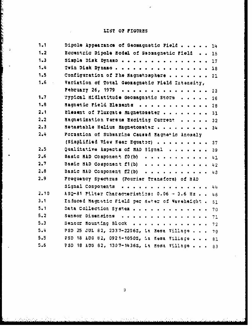
LIST O FIGURES

1.1 Dipole Appearance of Geomagnetic Field . . . * . 141.2 Eccentric Dipole Model of 3eomagnetic Field . . 151.3 Simple Disk Dynamo . . . . . . . . . . . . . . . 171.4 Twin Disk Dynamo. ....... . . . , . . . . 181.5 Configuration of The Magnetosphere . . . e . a . 211.6 Variation of Total Geomagnetic Field Iatensity,

February 26, 1979 . a a s v a * a e s a e a e a 23

1.7 Typical Midlatitude Geomagn3tic Storm . • • * ° 261.8 Magnetic Field Elements s . . . • . . e s e . . 282.1 Element of Fluxgate Magnetometer . . . . . . . . 312.2 Magnetization Versus ExCiti.g Current . • . * • 322.3 Metastable Helium Magnetomettr . . .s ° . . . 342.4 Formation of Submarine Caused Magnetic Anomaly

(Simplified View Rear Equator) a a s a a . e e . 37

2.5 Qualitative Aspects of MAD Signal * . . 392.6 Basic MAD Component fO(b) a . . .... • . • • 41

2.7 Basic M&D Component fl(b) • . • • . • .• • • 422.8 Basic MAD Component f2(b) . . . . . . . . . . . 432.9 Frequency Spectrum (Fourier Transform) of MAD

Signal Components . . . . . . . . . . .a .s Lj42.10 ASQ-81 Filter Chacac.eristi-s: 0.06 - 2.6 Hz . . 463.1 In.luced Magnt.tic Field per dwter of Waveheight . 515.1 Data Collection System . .. .. ... .. 705.2 Sensor Dimensions * * . ... . . 715.3 Sensor Mounting Block . . . • . • • . . a • . a 725.4 PSD 25 JUL 82, 2337-2206Z, La Mesa Village . . . 795.5 PSD 18 AOG 82, 0921-1050Z, La Mesa Village . . . 815.5 PSD 18 AUG 82, 1307-1436Z, L% Mesa Vi1lage . . * 83

ACKNO WLIDGEMESrS

Although many people contributed directly and indirectly

to this thesis, I owe a special gratitude to my ad-isors,

Dr. Otto Heinz and Dr. Andrev R. Ochadlick, Jr. for theirguidance, cooperation and assistance. I am also deeplyindebted to Mr. David F. Norman of the W. R. Church ComputerCenter, and other center personnel for assistance in the

"debugging of my computer software. Thanks is also due to

Dr. Paul H. Moose anI Dr. Michael Thomas for generalguidance, to CPT Edward Pogue, USA, for assistance in data

collect-ion, and to LCDR Arnold Gritzke, USN, and LT RobertJohnson, USN for their assembly of and assistance in docu-menting the PCM system.

10

A. HISTORY OF GEOZAGN-ETICS

The beginnings of the study of geomagnetism lie back inprehistory when magnetic attraction between iroa and certainminerals was first observed. Exactly when this phenomenonwas first noticed is not known, but the properties of magne-tite, then called lodestone, appeared in Greek literaturearound 600 B. C. (Brennan and Davis). [Ref. 1]

Chapman [Ref. 2] indicates that the directional propertyof magnets was known and ulsed in Europe prior to 1200 A. D.and possibly in China before then. E. N. Parker [Ref. 3]noted "It is an interesting fact that the ancient walls ofPeking were lined up with magnetic .aorth rather 1hangeographic north, a difference at that time of about 10. Wemay presume that the su-veyor found it easier to work withhis compass needle by day than to sight on the pole star bynight." This property allows the use of the Earth's geomag-netic field for navigatio4al purposes.

Dy the mid-fifteenth cant.ury .t was determined in Europethat the magnetic compass does not point to true north. Theangle between true north and the direction indicated by thecompass is now known as magretic declination by the geophy-sicist and as variation by the navigator.

The magnetic field dip, or magnetic inclination is theangle, in a vertical plane, between the horizontal and thedirection of the earth's magnetic field vector. It wasobserved in 1544 by an instrument maker in Nuremberg namedHartmann, and again by Robert Norman in London in 1581.

These discoveries or observations gave rise to "he studyof geomagnetics as a specialty which gainqi its cornerstone

Il

.......................

with Villiam Gilbert in 1600. After comparing his experi-

memtal results with the previous work of others suc" as

Niorman, Gilbert, in his book, 022 mJILSA B," concluded t.hat

"main mam a Ut q SkW jjn natij (the earth globe"itself is a great magnet)" [Ref. 2]. It is this concept,thet the earth is itself a magnet,, that is the basis of thescience of geomagnetics.

Gilbert felt that the Earth's magnetism must remainconstant except for geological changes, but it was soon

determined that this %as not the case. A 'secula. varia-tion' of the Earth's was found to exist.

Shorter term changes in the qeomagnetic field wereobserved and it was eventually realized that geomagnetism isdynamic. In 1722 George Lraham discovered that daily, ordiurnal, variations exist [Refo. 2] During the earlyNineteenth century magnetic observatories began to be estab-lished to record the chan;eg in the geomagnetic field in asystematic fashion (Knecht) [Ref. 14].

B. EARTH'S MAGNETIC FIELD

There are various ways of breaking down the consti-

tuting parts of the geomagne-tic fiell. One way is to divide

the field in terms of distance from the center of the earth.Doing this yields these three parts: internal, crustal, andexternal (AFGL) (Ref. 5]. The int~cnal field orlginat~s in

the core region and is the more stable field, containinqonly extremely low fraqu ncy temporal variations. Thecru_-.al (or anomalous) field arises from mod.ifications madeon the internal field by materials and structuras In theEarth's crust. These variations arg no spa tillly constant

and give rise to zome of what is known as geological

12

variations. The external field is the most dynamic andarises from many sources including the interaction betweenthe solar wind and the terrestrial magnetic field.

Another way of describing the components of thegeomagnetic field is by time variation. This division isaccomplished by considering that part of the field whichvaries with periodicities greater than about on% year as the"t jj..• ,,..214 and what is left as the n i(Knecht) . [aef. 4]

The st3ady field consists of the above namedinternal field, also referred to as the m . Slowvariations in the main field with periods of years or longer

are referred to as a

Various models of the main geomagnstic field makeuse of a geocentric dipole. Gauss, in 1839, demons:ratedthat, as a fairly good first approximation to the geomag-"netic field, the field of a uniformly magnetized sphere (forpoints outside the sphere) is q.uivilent to the field of amagnetic dipole located at the center of the sphere(Jacobs). [Ref. 6]

The simplest of the present approximations of thegeomagnetic field is that of a short bar magnet. or dipolelocated at the center of the earth with an axis inclinedapproximately 11.50 from the Earth's axis of rotation. Thesense of the field lines is from 3outh to north (Figure1.1) .

The axis of this dipole intersects the earth at thegeomagnetic north pole, 78. 50N, 291.0oE in geographic ccor-dinates, and at the geoaagnetic south polo., 78.5OS, 110.OOE.The moment of the geomagnetic dipols is 9.1 z 1022 amp-m 2 .it is these poles that are used to define the geomagnr.tic

13

wN

Figure 1. 1 Dipole kppearance of Gomatguetic Pield

coordinate system (Knecht) [Ref. 4]. The geomagnetic coor-dinats system is a spherical polar system similar to the

geographic coordinate system with a geomagnetic equator

defined 90 degrees away from either geomagnetic pole inlatitude, This tilý-ed geocentric dipole model describes th-s

maiin geomagnetic field to an accuracy of about 10%.

In 1940 Chapman aad Bartels defined -in off-cenrter

dipole in the earth's interior, called the eccentric dipcla.

This dipole is displaced 0.0685 earth radii (436 km) in

magnItude from the center a.nd in the lirection of th? point15.6ON, 150.90E (geographic coordina'es) (Vestine) [Ref. 7].

14~

[+

The intersections of the occent:ic dipole axis at the

earth's surface are 81.OOIV# 84&.70V and 75.OOS, 120.461

(Figure 1.2) (Haymes) (We. 8]. This approximation is accu-

rate to within a fey percent*

-0*

0, /oo ,W

Figure 1.2 Eccentric Dipole model of Geomagnetic Field

The field has additionally been modeled I.-o an accu-racy o abou 1% by determi.nining '"aassian coafficients by it

least-squares fit of experimental measurements of the

geomagnetic field. These coefficients are used in a spher-ical harmonic series representing the scalar potential ofthe field. This accuracy implies that the intsrtal contri-bution to the total main field is at least on the order of

-The International 3eomagnetic Reference Field (IGRF)yields values which differ by only parts per thousand from"measured values.

There are various elements that contribute to thegeomagnetic field, some external to the earth's surface andsome internal. As previously meationned, the external

contributions make up only a small fraction of the steadyfield, playing a more important role in the yjr!j!tjn.

These external sources include current systems inthe earth's upper atmosphere affected by solar electromag-netic radiation and gravitation, solir corpuscular radiationor the interaction of solar plasma with the main field, ani.the effect of the solar interplanqtary field. [Ref. 41

4 Various magnetic surveys of the world, includingthose con~ducted at grounl level, by airborne instruments,and by satellitehave pointid to the fact that the largestsource of the earth's magnetic field is intsrnal to it.While there exists resilual permanent magnetism in the

earth's crust, this cannot be ths p-'incipal internal sourceof the geomagnetic field due to temperaturs -nd material

properties known Xo 4xist in thG earth's int.rio: (NeaataadOzima). (Ref. 9]

and Permanent magnetism is generatid by microscopicelectric currents, siDce a changing e91,ctric fiel1 willgenerate a magnstic fiel,3. Another way to generate amagnetic field is by the motion of electric charges in a

[.6

:a

macroscopic current. Convective motion of the electrically

conducting fluid core of the earth, resulting in a macro-

scopic current system, is considered to be the principal

source of the main field.

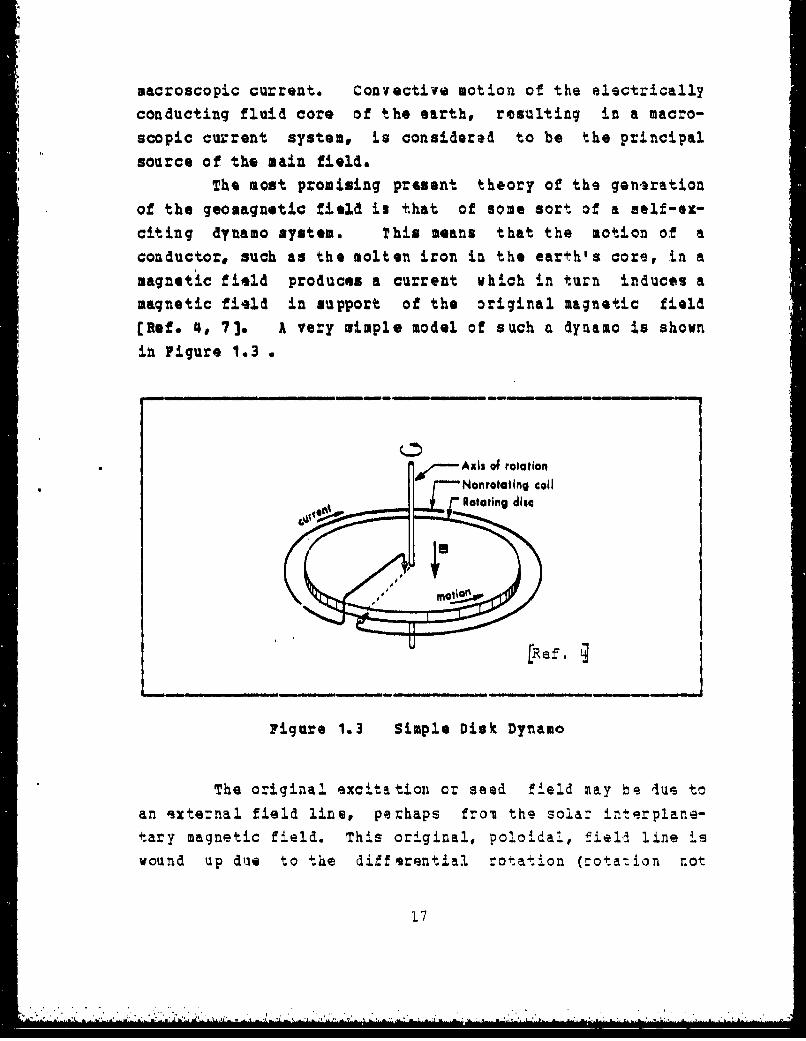
The most promising present theory of the geniration

of the geomagnetic field is that of some sort of a self-ex-

citing dynamo system. This means that the motion of a

conductor, such as the molten iron in the earth's core, in a

magnetic field produces a current which in turn induces a

magnetic field in support of the original magnetic field

[Ref. 4j, 7], a very simple model of such a dynamo is shown

in Figure 1.3

*,,,--Axis of rotation

Nonrotating coll

• II 1 /- m ot aio n g is

Figure 1.3 Simple Disk Dynamo

The original excitation or seed field may be 4ur toan external field line, perhaps from the solar interplane-tary magnetic field. This original, poloida!, field line is

wound up die to the differential rotation (rotation not

17

.. N -. .

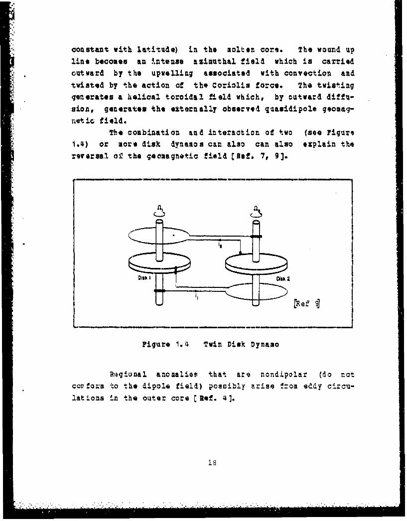
constant with latitude) Ln the Molten cor-. The wound up

line becomes an intense azimuthal field vhich is carried

outvard by the upwolling associated with convection and

twisted by the action of the Coriolis force. The twisting

generates a helical toroidal field which, by outward diffu-sioAn, generates the elternally observeod quasidipole geomag-netic field.

The combination &md interaction of two (see ?igurs1.4) or more disk dynamos can also can also explain theevwersal oS the geomagnotic field [Ram. 7, 9].

isk IDisk 2

[R ef 93

Pigure 1.4 Twin Disk Dynamo

a.gional anomalies that are nondipolar (do notcoriform to the dipole field) possibly arise t-om eddy circu-

lations in the outer core [Ref. 41.

I /

The aBMt•a• hs can be defined to be that region

(see ligure 1.5) occupied by the geomagnetic field above the

ionosphere, a region where the field stongly influences the

dynamics of ionized gas and charged particles (Kern)clef. 101.

If the space surrounding the earth were a perfect

vacuum, the 2arth's magnetosphere and magnetic field mightbe more or less symmetric and extend outward until it metqed

with, and its strength became insignificant compared to thesolar and other planetary magnetic fields. This turns outnot to be the case.

Zustead of being an island in a perfect vacuum, the

earth encounters a continuous flow of hot, highly conductiveionized cas, or plasma, streaming outward from the sun.This continous stream of charqed particles 1p called the

sglU 1ina. The density of this 'wind' near earth is on theorder of 10 particles per c=i, and has a velocity averaging300-500 km per second (Jacobs). [Ref. 61

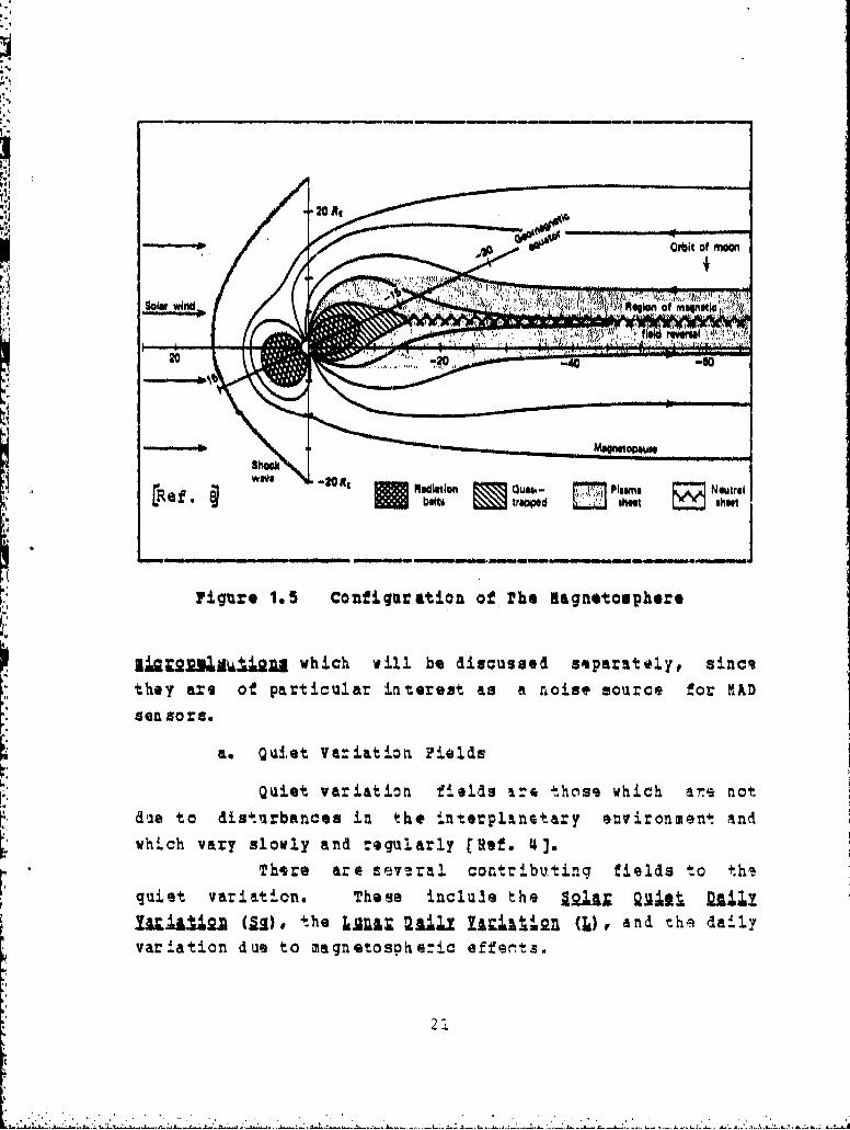
Both the solar wind and the geomagnetic field ixertpressure. The hot plasma of the solar wind pashes againstthe geomagnoftic field deforming the field. At distancesgreater than about 13 or 14 earth ralii, the pressure of thssolar wind greatly exceeds that of the geomagnetic field andthe geomagnetic field will be swept. along with the wind.From 8 to 10 earth radii inward, the geomagnetic fieldpressure will predominate, excluding the sola: windi, thisbeing the region of the 1•.U112EZ.

In the intermediate region, the magnitude of thesolar wind and geomagnetic field pressures are comparableand the solar wind is compressed and flows around thegeomagnetic field. This occurs when the magnetic energydinsity ahead of the plasma equals the kinetic energy

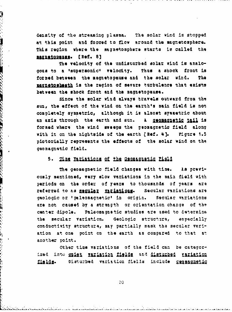
dens.l.ty of the streaming plasma. The solar wind is stoppedat this point and forced to flow around the magnetosphere.This region where the magnetosphere starts is called the

AUa loaa. [Hof. 83The velocity of the undisturbed solar wind is analo-

gous to a ,supersonic' velocity. Thus a shock front isformed between the magne•topause and the solar wind. ThejM.2n±%2obheah is the region of severe turbulence that existsbetween the shock front and the magnetopause.

Since the solar wind always travels outward from thesun, the effect of the wind on the earth's main field is not

completely symmetric, although it is almost symmetric aboutan axis through the earth and sun. A 22il9aiuj I isformed where the wind sweeps the ,geomagnetic field alongwith it on the nightside of the earth [ef. 4]. rigure 1.5pictorially represents the effects of the solar wind on thegeomagnetic field.

The geomagnetic field changes with time. An previ-

ously mentioned, very slow variations in the main field vith

periods on the order of years to thousands of years arereferred to as 6-4 la g 1 Ia±J Secular variations are

geologic or 'paleomagnetiac' in origin. Secular variationsare not caused by a strength or orientation change of th?center dipole. Paleomagnetic studies are used to dstermine

the secular variation. Geologic st:ucture•, especially

conductivity structure, may partially mask the secular vari-ation at one point on the earth as compared to that at

another point.Other time variations of the field can be categor-

4-zed into g~gj.j !UjjLt2.L 11gl1 and !" gkjYuL12=2• Ills. Disturbed variation fields include qq2MAqetjq

20

'I

I Nq~simn of mqntl

[RefUV -2CR At sdlation Quasi- Pama Nowtral

Figure 1.5 Contigaration of rho Magnetouphere

I±2~~g~.guwhich will] be discussed saparatelyr SinCI

the ataof particular interest as a noise source for MAD

a. Quiet Va:iation Fiel.ds

Quiet va~riation fields %: those which are notdi~e t o disturbances in tho interplanetary environment andwhich vary slowly and regularly rRef. 4].

There are several. contr ibuting fields to t hequiet variation. These include the 121gi

!AZU:U±2I (1g). , he Isnar U11 lzlt,2 (1), and the dailyvariation due to magnstospheric effernts.

22.

The Solar Quiet (Sq) variation is the name given

to the pattern of diurnal field variation with respect to

solar local time which is caused by currents flowing in the

ionosphere (Hatsushita) (Ref. 11]. ohe major portion (about

two-thirds) of the Sq field is due to what is referred as an

n•£AaahltMl 4ZA&I. . High speed tidal winds are generated by

solar heating causing con."ction of the upper atmosphere

[Ref. 41. These winds produce a stationary current system

by moving the conducting particles of the upper atmosphere

across the geomagnetic fikld lines. The daily variation is

caused by the earth rotating under the current system. The

remaining third of the Sq variation is caused by currents in

the earth induced by the primary curcents in the ionosphere.

"The sq field cin be shown to be latitude depan-

dent reachLng a maximum at the magnetic equator where a

concentration of current, the equatorial electrojet, exists

Ref. o4]. The maximum horizontal component intensit.y isabout 100 nT at the aquator with 25 to 50 nT more likely athigher latitudes.

Lor.gitudinal, seasonal, and solar cycle depen-dencies also occur for the Sq field.

an example of the gulet-day variation atMonterey, California 1:3 shown in Figure 1.6 and is summa-

tized in Table T. This lata was taken using a Cesium Vapor

total field magnetommte: in February, 1979.The Lunar Daily Variation, L, is approximately

one-tenth the magnitude o! the Sq field and exhibits t

sami-diurnal behavior in lunar timno [Ref. 4]. Thq majordifference is that the winds arv causad by lunar-eola-

gravitational tides. The L field 13s dependent on seasonal

influences, lunar phase, t'hq solar cycle, and latitude.

-TIM&

,1:

glg4 a'

I(

roll.,

Figure 1.6 Variation of Total Geomagnetic Field Intensity,February 26, 1979

a.

.1 . . , ; , ' ..

I MLE I

QUiet Day Variation in La Roum Villager Pobruarys, 26f 1979

POSITION 366361mN, 121*'S1'W (LA MESA VILLAGE)

CALCULATED VALUES USING TWO 197S U.S. CHART MODEL CWO*LD DATACENTER As BOULDER, COLORADO) FOR FEBRUARY 1971:

D I N(NT) ZcNT) F(14?)2VALUE (FEB1. 1979): 15.960 60.740* 21.,60 441,007 50,41.1

MARLY CHANG1 : 2.5 1 - .$ I a.3 -52.1 -30.1

HIMASURED VALUES OP TOTAL FIELD INTENSITY FOR FEB. 15p 1979

*DAIS TINS PcNI)

3/15/79 00eat($ 50,1.05.21.91:1.0 50.1405.79

@1:52 50,31.59.S

13:21 50,3308..31 4 - O05:00 50.1.00.1910,:06 50JI80.156

00:12 0,399.9109:10 0,301.85

20:20 50,505.1011:207 $0,400.540 O

2/6 012:2 50,3306.51 MI.A

AVE:AG 50,350.1.0 2.3C

11L MES $.53 N0,3R .10

251. 4S309

A diurnal effect due to the dayside-nightside

difference in compression by the solar wind of the geomag-

netic field causes a small variation of the oerda of 3 nT

[Ref. 41.

b. Disturbed Variation Fiells

21atiibaa d y EiLka9a •lili.j are geomagnetic field

variations that appear to be the result of iaterplanetary

environmental changes and do not possess a simple period-icity. These variations include 122§29hXI U IUI.• nAI,the aBIgIAu, .oaraLO s, and gainugiU

An Eb*2 r M&%;g&1 is a daparturs fromthe normal behavior of the ionosphere.

SQU ITL. j ttgit. (Itll are magnetic distur-

bances produced by X-rays emitted from the solar flare.

SFE's usually have a rapid onset, typically a few minutes in

duration, followed by a slower return to normal. The entire

event lasts on the order of an hour (Reird). [Ref. 12]

Ir~a§ are c aused by +!he precipitation ofcharged particles down magnetic field lines into the atmos-

phere and can be one of the brightest visual phenomena intha sky. The more intense and active auroras occur withgeomagnetic disturbances and greatly increase cnizaticn as

well as creating the spectactular visual displays. [Ref. 4]

2qo|gstS j•ras are due to a change in thedynamic pressure of the solar win4. A typical storm begins

with a compression of the magnetic field by an increase insolar wind dynamic pressure called a jgA •a.J.gI... .

(S), .high Increases the magnetiý field (Tas so-called"gradual storm" begins with a gralual increase in fielistrength). The increase in field strength is on the order

of several tons of nanoTeslas (nT) and takes about one to

25

six minutes to rise. If a disturban-e ntarts with an SC butlacks the succeeding stages of a storm it is referred to as

a RU4= In"l&i (1I). Following the SC, the field remainscompressed for two to eight hours in the initLl v ofthe storm. The a"& 2kag follows the ij.itial phase. Overa period of hours to a day a westward ring current is set upat a distance of several earth radii whose magnetic fieldleads to a decrease in field stren;th on the order of 100"nT. This decrease overshoots the aqiilibrium field, atrengthand leads into the rL.suqrX ALn of a day or longer vwhtrethe field returns towards its prestorm strength as the ring

currents gradually dissipate [Ref. 14), (Matsushita).• riefo 131, a magnitude-.time graph of a typical gesomagnetic

storm is shown in Figure I.%.

AH

phaw

Main pheas• , Rucovery phiw a-+... w= Time

Sudden commuicemon"t,

S.C..

*--20c £Ref.

Pigure 1.7 Typical didlatitude Geomagnetic Storm

.. .

MUMA9 L22 912ni are rapid fluctua-tions in the surface magnetic field with periods of about

0.2 seconds to 10 minutes (frequencies about 0.0016 to 5.0

Hz. These are observed as a type of geomagnetic distur-

ban ce by ground based magnetometers E Relf. ].

Micropulsations will be discussed in depth later.

The geomagnetic field vector is measirsd or charac-

terized at any point by its direction and magnitude. This

can be done in terms of some set of three independent param-

eters such as two direction angles and the magnitude, or

three perpendicalar components. [Ref. 4]

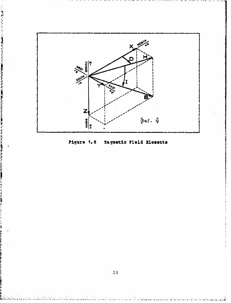
The system of coordinates commonly employed for

describing the geomagnetic field on the surface of the earth

is shown in Figure 1.8. The field is measured in terms o!local (geodetic) coordinatos with raspect to True North.

The various coordinaates are referred to as jascne+•

2j_9,.. t,,. and are defined as eollows:A: Total Field Intensity (the symbol Z is

also used)J: Horizontal Component

X: Northward, or North-South Component

1: Eastward, or East-Wast ComponentZ: Downward, or Vertical Componqnt" 2: Declination or magnetic variation."This is the angle betwee.s j and • and is

measured positive eastward.J: Inclination or dip angle. This is the

angle between a and • and is aeasuredpositive downward.

17.27

1±gure 1.8 !1aguetic Field Elements

u%28

A. DEFINITION OF k MAGNETIC ANOMALY

A magnetic anomaly is defined as any spatial variationor disturbance in the geomagnetic field which is due tolocal causes. Anomalies can be caused by waves, oredepositas, sea mounts, and magnetized objects such as surface

ships and submarines (Anderson) aest. 14]. For the purposesof this research, magnetic anomalies due to a simple dipole

field, such as those generated by submarines, will beregarded as signals, while other anomalies will be regardedas noise and will be discussed later.

B. H73TORICAl DEVELOPMENT OF THE MAGNETIC DETECTION OFSUBMARINES

Attempts at finding submerged submarines by sensingdisturbances in the geomagnetic field date back as least asfar as World gar I. In 1918, Earnest lerritt, at the NavalExperimental Station, New London studied the use of a fixedcoil type of detector for 4se in moving boats and airplanes(Slichter). [Ref. 15]

MAD, originally known as Magnetic Airborne Detector,and now called Magnetic Anomaly Detection, hal its begin-nings as an airborne ASW sensor in late 1940 and early 194,1.

Anomalies in the geomagnetic field caused by thepresence of submarines, are )n the order of one to a few nT(gammas) in magnitude. This is quite small compared to themagnitude of the field itself (30000 - 60001 nT). rwomethods are generally gmployed to measure this small

29

disturbance. One is to use a gra1oti. which measures the

spatial rate of change of the magnetic field or its

a/4dijn•. The second method, and the one presently used byU.S. Navy aircraft is to use a |.e +.qotL to directlymeasure changes in the magnitude of the magnetic field.

The British investigated the use of a gradiometerfor submarine detection, &nd by early 1941, had developed atwo-coil gradiometer system which could detect a submarineat a range of 200 feet under favorable conditions. Thisrange was considered to be too small to be of operationalvalue and work on such a system was terminated when a magne-tometer system showed promise (Coleman). [Ref. 16]

By late 1940, Victor V. Vacquier of the GulfResearch and Development Company had developed a sensitivegqt_ l jgjog magnetome ter intended for geophysical(mineral) prospecting. The Vacquier mr gnstometer became th4basis for further MAD development. The Airborne InstrumentLalboratory of Columbia University continued the investiga-tion of means of localizing submerged submarines by MAD.

The simplest saturable core or fluxgate magnetometerconsists of a saturable or ferromagnetic core around which acoil of wire is wrapped (see Pigure 2.1). This coil ca.riesa sinusoidal current, I(t), which is large enough to satu-rate the core during part of each cycle. The inductance ofthe coil will change as a function of the magnetization ofthe core. The core magnetization, i turn, dapends on theinstantaneous cuzrent, in the coil, and, if present, the

exteonrl magnetic field.

In the absence of an extgrnally applied magneticfield, magnetization as a function of exciting current issymmetric around 1=0 (Vgtire 2.2). An external magneticfield parallel o the core' s axis will chanqe the magneqtza-tion of the core and shift -he magnstization curve. This

-I

Primary

N Excioti. n

a, Secondary

Itm,

q"cI

N1 I I j N Ambii Field

Figure 2.1 Element of Fluxgate Eagnetometer*4

chauqg will cause an asymmetry which can be sensed by

analyzing the harmonic content of the signal. The coil can

be combined with a stabilizer system# which keeps thq

detector olement (coil) aligned with the geomagnetic field.

This was the basis of the MAD magnstometers used inWorld War 1I such as the AN/&SQ-1, ISQ-1A, and ASQ-2

[Rof. 16].The fluxgate magnetometer measures only the ccmpo-

nent of the external field parallel to the axis of the

ferromagn.tic core. In ocder to measure the total field inthis fashion it is necessary to align the firromagnetic cors

4 along 4:h4 earth's maqnet ic f ield or by using mu-vually

-31

SI'-• . . . . . . . . .4 14 4 * * 4 - *** * ' * . I **,

figure 2.2 Ragnetization Versus Exciting Cairent

I.h

per pendicular (orthoqonall cores. precision requir:ement$

made this type of ~system difficult to realize duaring WorldWar 11 but it his since found many years of operational

usage and has found widespread use In geophysical explora-ti.on work and satellite mapping of the geomagnetic field.

During World War 11 MAD proviled a passive mnethod of

detection and tracking of submerged submarines. Within its

range (then on the order of 500 feat) MAD gave a measure of

surprise to the attacking aircrew. U~ntil. the first attack

was delivered the crew of t.he submerged suibmarine ml-ght not

even be avars of the aircraft hunting it.

operational deployment of MAD began on a limited

basts in December,, 19(41 with the installation of the early

Mark I MAD in a blimp at Naval Air Station Lakehur-str New

Jersey [Ref. 16].

3

q3

-4•r

. .

By the end of 1942, MAD was Dpe-ational on board PBY

Catalina aircraft, nicknamed "Hadcats." Even though HAD wasoperational at this time, it was not until February# 1944

that an initial contact by MAD led to the sinking of asubmarine.

Durinq February, 1944, the Madcats of PatrolSquadron 63 were assigned to fly a HAD barrier patrol of the

straits of Gibraltar. On 24 February 1944, a Madcat ofVP-63 detected U-761 by use of MAD and commenced tracking to

confirm the contact as a moving target. In attack was

conducted in conjunction with another Catalina, two

destroyers, and eventually two other aircraft# and U-761 wassunk. U-392 was sunk after a similar HAD contact on 16March, and on 5 May, the third successful attack on a U-boatresulting from an initial HAD contact took place when U-731was sunk (OEG No. 51, Price). [Ref. 17, 18]

The attacks at the Straits of Gibraltar demonstrated

that though MAD ý±s a limited search rat-, there artscenarios where it can be employed effectively as a searchsensor, such as providing a blockade across a restricted

area without the presence of surface craft (33G No. 54)[Ref. 193.

The magnetometer system in current operational use

is the optically pumped magnetometer. The optically pumpedmagnetometer measures the external nagnetic field by makinguse of the fact that when an atom is immersed in a magneticfield, its energy levels are split. This is known as theZeeman effa.. For the fields of interest, the amount ofsplitting of the levels is proportiinal to the intensity ofthe magnetic field. By measuring the separation between thslevels the magnitude of -he magne-ic field can be

det-?rmined.

33

This type of magnetometa:- usually makes use ofcesiu, or Rubidium, vapors, or Helium gas. The current oper-ational HAD system, the AN/ASQ-81,, is a Helium gas Opticallypumped magnstometer.

1~w in an optically pumped magtotometer (soe Figure2.3),, the sample vapor or gas (such as Helium) is collectedinto an absorption cell. Circularly polarized light ispassed through the cell giving up some of its energy inexciting or pumping the electrons of the sample gas tohigher energy levels. These 4lectrons then fluoresce tolover, metastable energy states. T!his is 'optical pumping.'A detector monitors the degree of optical pumping by meas-

uring the transparency of the gas usll.

IILigh I I Al

.bbeepe Imetal

/ I

Figure 2.3 Metastable Helium Magnetometer

The actual separation of thse ~aergy levels is mieas-

tired by applying a weak R. P. field which redistributes ths

34.1

electrons among the ground state sublevels. These tran-sitions will only occur when the R. P. field has a partic-

-, zular frequency (callel the Larmor frequency) which isproportional to the separation between the levels and there-

fore to the external magnetic field [Ret. 203. Thus meas-urement of this frequency yields a direct value of the

magnetic field.14.

Optically pumped magnetometars are the most setsi-

tire Mensor for fleet usage today. Increasing oapability to

_ make use of the phenomenon of super.onductivity will yieldmore sensitive HIAD sensors. Sape'conducting ' quantum

Interference Devices (S500IDS) which make use of theJosephson effect have a theoretical sensitivity of 10-7 nT

as opposed to the theoretical value of 0.001 nT and theopez~aticnally realized value of 0.01 nT in current flset

systems (Chilton) [Ref. 203. Field changes on the order of

10-5 nT have actually been measured. This SQUIDS are usedin both superconducting magnetometers, and superconductinq

gra diometers.

A Josephson junction consists of a thin layer of

insulator between two superconductors. This Junction hasthe property that a current can flow across it without"developing a voltage up to some maxisum current. A voltageis developed for all current values greater than the maximum

Current.

in a superconducting magnetometer a superconductingring containing a pair of Josephson junctions is used tomeasure the amount of magnetic flux p9netrating the loop.This system is a vector magnitomister which meaeurrds varia-

tions in only one field component.

:4

4,, 35

*1

By using more than one superconducting loop, it ispossible -to measure magnetic field gradients, ind construct

a superconducting gradiometer. This is also a -omponent, orvector, sensor.

These instruments have been used extensively in the

laboratory and to some extent in geophysical work, butconsiderable engineering probleas remain to be solved before

operational Navy use can be contemplated.

C. BAD SIGNAL AND BANDPASS

The MAD signal results from moving a magnetometerthrough the magnetic field of a submarine, which can beapproximated Ly the field of a magnetic dipole. ?Lgure 2.4depicts the formation of a submarine caused anomaly.

The magnetic moment of an object in the earth'smagnetic tield can be due to parmanent magnetization,magnetization induced by the earth's magnetic field, or a

N combination of both. In the case of a submarine hull both

causes are present with a small amount of permanentmagnetization produced by hull stress in metal componentsduring construction and stress caused by submarine divingand surfacing. This, however, is a minor contribution. Themost important constituent of the submarine magnetic momentis due to magnetization induced in the hull by the presenceof the geomagnetic field. (Ref. 21J

The induced field of a submarine depends on theeffectiv- permeability along the vertical, athwartships, andlongitudinal axes of the snbmar4 .ne. This information ,

taken togelher with the strength and dip anqle of "•hageomaqn.tic field, yiells a fairly preciso cai t.u ion ofthe magnetic anomaly produced by the submarine. 'Depermiung

36

%I,

V3 CD

•1:311

Figure 2.4 Poimationeof,,ubmarine Cansed Magnetic Anomaly

(S mplifi d sQw Near Eqat.or)

37

• .• .,- ,- -•. ..... , .. . , ,.,. • . ." .. .... ..:.. .. ., .' .. .,•. ' r,. .... ... -. .. .• .f . ..'. .. . .. . . ,)"

of the submarine hull cancels out the permanent hull

magtetization leaving the induced magnetization as +...eprincipal signal source. CRef. 21]

The HAD signal is approximated as the projection ofthe submarine dipole field onto the qeomagnetic fieldvector. This approximation is good because the magnitude ofthe dipole field is very much smaller than the maqnitude of

the geomagnetic field (a few nanorsslas as opposed toapproximately 50000 nT). Therefore, whenever the dipolefield is perpendicular to the earth's field a region of zerosignal will result. The signal recorded by the AN/ASQ-81 orother HAD equipment is a mapping along the aircraft's flightpath of this signal. Figure 2.5 qualitatively describessome aspects of the MAD signal.

2. 41a9so Msg1212

The submarine anomaly signal shape is a function ofthe dip angle of the geomagnetic field, the magnetic headingof the aircraft, magnetic heading Df the submarine dipole,and the lateral range between the aircraft and the subma-rine. These factors detwermine the 'A' coefficients for thheAnderson functions below.

In 1949# J. E. Anderson of the Naval Air DevelopmentCenter determined that the MAD signal, obtained along anycourse, consisted cf a linear combination of three basiccomponents. Different shaped signals could by changing theproportionsl contribution of these basic componnats. Thamathematical representation of these components are now

referred to as the Anderson functions. using the dimqnsion-less parameter IbI (4efined as the li~sance traveled alongthe aircraft track divided by the slant range at clos.s-point of approach (CPA), b=O at -PA) the anomaly can berepresented by

38

,'loft S;Sp*&

Fiur 2s. 5 Ultt~ Set tMDSga

I

---

Figure 2.5 Qualitative Aspects of MAD Signal

39

S A2 b 2 + Al b +.0Ba -e .....- -- ------------ (2- 1 a)

Z3 (bg +1) 5/2

or: Is Z [1O fU (b) + A1 fI(b) + &2 f 2(b) (2-1b)

vheze • W magnetic moment of target dipoleZ - lateral range between target and plane &t CPA

f0 (b) "-------------- .....

(b2 +1)5/2

bf I (b) -e e

5/2(b2 b 1)

f2 (b) a . . . . . . .5/7.jb2 + 1)

The strength of the detected siqnal is seen to falloff as the cube of the distance between the a&!.rcraft and thetarget.

B7 analyzing tha functions and their coefficients,it can be shown that the optimum orientation for maximum

anomaly signal detection is when the aircraft, ta-getdipole, and geomagnetic field are lined up togather asclosely as possinle. Specifically, this occurs when thesubmarine moment and the aircraft s track ire oriented

North-South. [Ref. 14,. 21]

The Fourier transform of the component functionswere taken to determine the frequency distribution of snergy!.n the MAD signal. The anomaly signal components are showni. Figures 2.6 through 2.6 (Anderson) (Rif. 14]. TheFourier transforms of th•. signal components with a platformvetoc ity of 150 knots are shown In Figure 2.9.

"40

I

* Es.

I

.4 1

I.4,

* g

N *

44* I I

1AA

I, �NN'4

'-4

I � --

Figure 2�6 3asi� lAD Component fO(b)

LIj

I

4

* k"b 1 - * 'I - - *

.@ .'.�

qm

4.

C)J.

'.4

4

-� q44

��4'-I

4-

I

A �'iqure 2.7 Basic Mu) Cou�ponent fl(b)

42

4

- 4 . - , 4 4 4 4 - . . . . - . 4 4

L1L

-43

N

IOU 0400

Figure 2.9 Floqena Spetru (F oure rasom)o II gnlCopnet44 IIA' P 2b

The HAD signal, being a transient, is essentially a

broadband (as opposed to a discrete frequency) signal. The

frequency spectra of energy content showh how the signal is

contained in a certain frequency riange. Tn order to screen

out unwanted noise, bandpass filtering is used in processing

magnetic anomaly detections.

The major factors influencing the determination of

an optimum MAD filter ftequency are aircraft speed and the

slant range from the aircraft to the target at CPA. Factors

exerting a minor influence include dip angle, aircraft

heading, and target dipole orisnzati~n.

The range in frequency variation is about an octave,

with the higher values occuring when the passes are made

parallel to the axic of the dipole and the lower when thepass is perpendicular to the dipole. Anderson qmpirically

determined that the center frequency of the filter is given

by

0.4 'f ., . . . . . . (2 - 2 )

where f f frequency in Hertzv * aircraift vel city in ft/secand Z U greatq t au+ ncipated CPA

range in feet

The ASQ-81 Bandpass Filter has highpass settings of

0.04, 0.06, 0.08, and 0.1 Hz, and Lwpass settings of 0.2,

0.41, 0.6, and 2.0 Hz (Orion Servica Digest 26) CRef. 22].

There are no recommended settings for normal operation sincq

background noise varies. the filter characteristics for the.

0.06 to 0.6 Hz settings are shown in Figure 2.10 (OrIon

Service Digest 28) (Ref. 23 3.

45

The figure is a representation of tbh adjustable band pass

C filter of the ASQ-81 by itself. Other patts ol the &SQ-81

system add in an additional high pass fil'ter which addsanother 12 dB/octave roll off to the low frequency end in

Figure 2.10. Thus Figure 2.10 would represent the charac-

teristics of the entire ASQ-81 system it +.he roll oft cuf 36

"'iBoctave is changed to 48 dB/octave. CRef. 241

14 Ref2

36 dO PER

RELAflVE OCTAVE'•"'+,,,, ILA'rVI .REJECTION

24do PER

OCTAVER -REJECTION

0,0? 0.1. 1i4 PREUINCY IN Ha

Figure 2.10 ASQ-81 Filter Characteristics: 0.06- 0.6 Hz

Using equation 2-2, the center frequency for a MAD

signal with a CPA slant range of 300 feet and a.rcraftvelocity of 220 knots is 0.49 Hz. Using a lowpass filter

setting above 0.6 Hz would not be very useful.Onr reason the ASQ-81 filter extends up to 2.0 Hz

instead of just 0.6 Hz is the following. The early ServicsTest Engineering Model (STEM) ASQ-81 that preceed'3d the

146

current ASQ-81 production model had two bandpass filters,

one adjustable from .04 to .6 Oz,, and the other fixed at .75

to 10 Hz. During tesat, the .75 to 10 Rz channel proved to

be helpfal in monitoring the STEM ASQ-81 "system" noiselevel. During design reviews for" the production ASQ-81, it

was decided that it might be uaeefal to retain the ability to

monitor "system" noise. rn or.eý- to do this easily, the .75to 10 Hz band was dropped and a 2 Hz position was added tothe adjustable filter. (Ref. 24]

The center frequency at 1200 feet. and 160 knots is

.09 Hz. Consequently, the highpass filter settings could

aff.ect slower, longer range R&D detections.ThQ choice of the highpass (lover end of bandpass)

sattings have to be made after considering ths noise presentat time of system operation.

47-. ,,,

&A. I1TODUCTION

"On a practical level MAD noise ts defined as magnetic

disturbances falling within ths K&D passban&. (0.04 to 2.0Sz, or aLnce 0.6 Hz is the normal upper limit, 0.04 to 0.6Hz) and having an amplitude greater than 0.01 nFnAOTeulas(the system sensitivity of the AN/&SQ-i1 HID system).

'e MAD noise sources can be diviled into the followingCategories:

-squipment Noisei-Aircraft Platform Noise-Aircraft danuever Noise-Gradient 4oise Due to Aircraft Notion Through the

-Geologic N01 .se-Noise from Wind Waves &nd Swells-Geomagnetic Noise

B. SEINSOR, PLAT?ORM AND MANUIVTR NOrSS

Sensor noise is the self-noise generated by the opqra-

tion of the equipment itself. This can be partially due tothe fact that the det-ctor elqJ•tt is mistliqned withrespect to the geomagnetic field vector. Changes in lampintensity, photodetector noise and noise in the electroniccircuits can also contribute to sensor noise [Ref. 21). The

self-noise limitation of the ASO-81 is 0.01 nT.

Platform noisa is qenerated by Components fixed to the

aircraft in the vicinity of h•t sensor (Ref. 23].Per.manent., induced and iddy-currant magnetic fields ari

48

associated with the airframe. Permanent magnitic fields are

due to aircraft structure or equipment having ferromagnetia"parts. This field changes its orientation with respect tot the geomagnetic field vector as the aircraft manuevers,causing field fluctuations near the magnetoaeter.

Platform noise is also induced in aircraft f6r=omagneticstructures by he geomagnst-c field. Similarly, eddy-cur-

ren 1s- are Induced in aircraft skin, ribap and frames,, andthese currents . in turn, cause additional magnetic fields.Thas, rapid aircraf-t , manuevers will induce changes in themagnetic field sensed by the magnetometer.

Platform noise in aircraft Mounted sensors is counteredby applying equal and opposite magnetic fields to the sensorin a process called compensation. Towed MAD systems are

weentially fre from this type of noise.

C. GRADIENT NO1SZ

Gradient noise can be divided into turn noise and noisedue to changes in altitude.

Turn nolse is a probleim when 'SAD trapping' or 11sing HAD

for tracking a target. The earth's magnetic field has ahorizontal gradiont (in this case the magnitude varying withlatitude). As t.he aircraft moves in the direction of thq

gradient the fi.eld strength changes. The roise due to a 8ADtzapping or hunting circla is centered in trequency at thereciprocal of the time taken to complete one revolution. In

the case of a two-winut-w circle, the nois woald be cenrtered

at 0.00333 Hz, well below the tilto~r used in the kSQG-81.

The Lorizontal gradient noise due to f.lying a cloverleafpattern, for the most part, also falls below 'th NOAD

possbard. (Ref, 21]VertIcal gradient noi-e is dae to changes in sensor

Salt 1ýtude. In altitude gradiant of 'ip to 0.005 to 0.01 tT

II. III9

per foot exists in the earth's main field. In areas ofgeological anomalies this gradient is even larger. Pastaltitude or aircraft pitch changes can cause a magnetic

K. field fluctuation of sufficient amplitude to be of concern.

To avoid vertical gradient noise, altitude compensation"II equipment is used. (Ref. 23]

D. ENVIRONNINTAL NOISI

magnetic noise from sources %xisting in the natural

environment include geologic noise, temaporal variation inthe earth's magnetic field, and noise due to ocean waves and

swells.Geologic noise has its source in naturally occuring

magnetic anomalies caused by magnetic material p.esent inthe earth's crust. When thb sensor passes over gqologicalanomalies, the relative motion causes a MAD-liks signal tobe recorded. Geologic noise is usually move pronounced inshallow water as the sensor is much closer to the source of

the noise. Geological magnetic anomalies ar. often associ-

ated with such oceanographic features as seamounts and oceanridqgs.

SPa wak-r is a conducting mediunm which is transported by

the phyiical motioTi of water wav-ze kan ýh.h presencs of thegeomagrietic fiqld. This m:tion inductas currents in the sea.These currents give Zise to secondary magnstic fields, whichadd vectorially to the quasistat ic, geomagnetic field(Weaver) CRef 25]. Thrse fields can be detected at signif-

icant distances above the sea surface anl fall off axponen-tially with altitude. ig'i=e 3.1 is a plot for several

sur'face wave pe:iods of the induced magnetic field per meter

amplitude of th., surface wvve.. These induced fiqldiý cdn bea problem at the low altitudes where 4AD is usod.

.50

'9 ,. 9

'IT

1 11i* H I 1 4 W.

W4+ 441A Sam Sari- *l t

Figure~~ ~ ~ ~ 3. indce Maqeti Field pe mee f0aaii

E. GEONAGNSTIC NOISE

Temporal variations in t.he earth's magnetic field with

frequencies in the MAD bandpass and amplitudes greater than0.01 nT have become known as gQItLga.%a1 nogIlz in the KID

literature.Quiet daily variations, such as the Sq and L variations,

have periods sufficiently long to fall far below the HAD

passband.Goomaqnetic storms have been discussed previously.

Rapid fluctuations with high amplitude and falling withinthe MAD passband occur in connection with geomagneticstorms.

S~ comprise the laest categoryof geomagnetic noise to be discussed.

Geomagnetic micropulsations are rapid fluctuationsof the earth's magnetic field with periods from 0.2 secondsto 10 minutes and amplitudes from about 0.1 nT to as high asa few tins of nT's. These fluctuations are caused by elec-

tromagnetic perturbations propagating in the magnetosphereas hydromagnet.c waves (Nishida). [Ref. 26)

Micropulsations ace classifiad by morphology, thatis, by examining periods, ampliltudes, times of occurence and

other observed characteristics. nicropulsations have beenplaced into two broad categories: I uL and 22.1a2222.The irregular pulsations are represented by the symbol Pi,and the continuous pulsations by Pc. Table II shows thebreakdown by period of the various micropuasat!nn classes.

It can be seen that for MAD geomagnetic noise the

lower frequency Pcl, Pc2, Pc3, and Pil pulsations are of

interest.

52

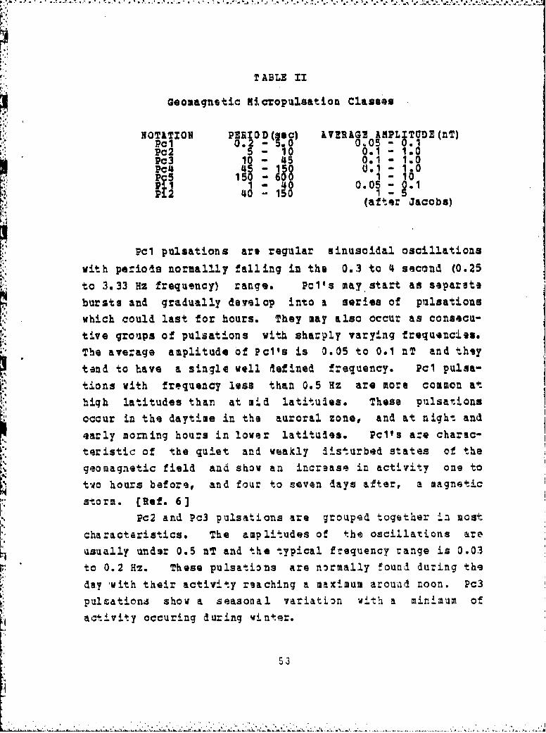
T ABLE II

Geomagnetic Nicropulsation Classes

NOTATION PERIOD( e & VERAGE ALIPLJTD (nT)Pc 0.2 0 o.o5 o 1

Soiii0 1.0

P 2 40 1501(after Jacobs)

Pcl pulsations are regular sinusoidal oscillations

with periods normalily falling in the 0.3 to 4 second (0.25to 3.33 Hz frequency) range. Pell$ may'start as separate

bursts and gradually develop into & series of pulsationswhich could last for hours. They may also occur as consecu-

tive groups of pulsations with sharply varying frequencies.The average amplitude of Pct's is 0.05 to 0.1 nT and they

tand to have a single well Aefined frequency. Pc, pulsa-

tions with frequency less than 0.5 Hz are more common athigh latitudes than at mid latitudes. These pulsations

occur in the daytime in the auroral zone, and at night and

early morning hours in lower latitudes. PcI~s a&. charac-teristic of the quiet and weakly disturbed states of thegeomagnetic field and show an increase in activity one to

two hours before, and four to seven days after, a magneticstorm. [Ref. 6]

Pc2 and Pc3 pulsations are grouped together il most

characteristics. The amplitudes ol the oscillations are

usually under 0.5 nT and the typical frequency range is 0.03to 0.2 H%. These pulsations are normally found during the

day with their activity reaching a miximum arouar noon. Pc3

pulsations show a seasonal variation with a minimum of

activity occuring during winter.

Li•

k"

Pc4 and Pc5 are large amplitude fluctuations, butfall below the frequency band of interest for HAD.

P.4 pulsations 4%ve an ir-egular form with anaverage amplitude of 0.01 to 0.1 nT and a frequency mainlyin the 0.10 to 0.17 Hz range. Speztral analysis of thesepulsatione show a braod band of freqaencies. Pil amplitudes

have maximum values in the auroral zones, with the intensityof the puIsations decreasing with decreasing latitude.Pil's are normally observed in the late night and earlymorning hours, and show an increase in activity withincreased geomagnetic field disturbance. CH-!,. 6]

Geomagnetic micropulsations can be observed anywhere:n 'lhe globe, at various 1imes of day and year, and in bothquiet and disturbed geomagnetic field conditions.

Iý

k. INTRODUCTION

Previous chapters hive defined geomi:.t'netic activity as

it applies to Hagnetic Anomaly Detection. In this chapter,

methods of evaluating that activity vill be examined,

including m'thods currently in use by the f'.eet.

B. GROIAGNETIC INDICES

A geomagnetic index is simply a measure used to quantify

and describe time variations of the earth's magnetic fieldresulting from solar-trerrestrial relationships. These

indices are commonly used to expresr the intensity anddepict the character of goxmagn4tic activity throughout the

day.For the most part, geomagneti. indices developed as

range indices, measurtng the difference between the high andlow values for different field components measured duringthe day by magnetic observatories (Lincoln) [Ref. 271. Most

cvtrent indices are of the range type, but other indices

have been developed which are more subjective o: qualitativein nature.

Geumaonetic indices are designated by a letter code suchas: C, Ci, Cp, C9, Q, R, W measura, Dex, K, Ns, Kp, ak, Akv

ap, and Ap. There are additonal indices in use.

The C, Ci, Cp, and C9 indices are daily magnetic fieldcharacter figures. The C index is the daily characterfigure for a single observatory. la this scale, C=O indi-

cates a quiet day, C=I a moderately 11sturbed day, and C=2 a

heavily disturbed day. The daily international character

55

fia'ire, Ci, is tho arithmetic mean of the C indices raportedby participating bseervatories around the worldi. Cp# -the

daily planetary character figure, is simila: to Ci, exceptthat it is derived from the valuos of Kp and ap. C9 is acontracted scale for Ci an Cp vith single diyit valuesronaing from 0 to 9 (Bartels). [Mf. 26]..

The Q and R indices are quarter-hoirly and hourly.rangeindl.cts ro3ayectively, taken at high latitude stations only.

The V measurm is an index of the equatorial electrojeo.,Dot is a measure of ring current effect. They a4..e bothamplitude indices. (Ref. 27]

The K, Ks, Xp, ah, Ak, ap, and Ap indices comprise a

group of related 3-1.our range indics., The K index is asingle statIon code using a quasi-logarithmic scale '.rom 0to 9 to measure geomagnetic activity. The value of K is

determined by first determlning the difference between thelowest and highest deviations from the regular daily varia-tion (Sq) during a 3-hour period. This range (in sT) isconverted to the K scale based on hhe historical activityranqes at the particular observatory involved [Ref. 27].The conversion for the Fredericksburg, Virginia observatoryia given in Table III. This conversion can also be appliedPo the USA?/NOAA observatory in aoulder, Colorado (Ref. 29].

The Ks index is a standardized K irdex which isfraed from local variations and is then uised to det.ermire

the planetary 3-hour index, Kp.The equivalent three-hour-range, ak, is a conversion

of the K index as shown .n Table 17. in order to d•emine

the units of ak for a particular observatory, divide thelower range limit of K=9 by 250. Thus for Fredericksburg

and 3ouider, ak is in 2-nT units.

"ovesnfoTABLE III

Conversion from Range to K for Predericksburg, Va.

K~R& nge IT)0 A

12 1 •: 013 -20:4O

•. . ,. (after Lincoln)

TABLE I1

Equivalent. Range ak for Given K

K 0 1 2 3 4 5 6 7 8 9alc 0 3 7 15 27 L48- 80 140 J400 400

(after LLncoln)

Ak i1 the equivilent laily amplttd•d and is th'.

average of the eight daily ak values at a particular obsev-

atory. This index is promulgated using the name of theobservat.ory, the Ik index fc'r ?redericksburg is known Rs t.hs

A-Fredericksburg or A-Fred index.The equivalent planetary amplitude,, ap, is det.•r-

mined f om the Kp index in a fashion similar to that o.

determining ak from the K indices. The eight ap valuas for

a given day can then be averaged into the daily equivalent

planetary amplituie Ap. These two Jniices arv given in 2-nTunits.

57

<: 2 ii5

C. GEONIGNETIC INDICES IN ?LEST USE

Geonagnetic indices of interest in connection withKID operatioAS are the Ko. Ak# and Ap indices.

Pleet operators atilize, the Nalpha Index' forperdictitng geomagnetic ictivity ,over the enti:9 world(Ref. 30). This indrox is promulagated by the PleatNumerical Ocenaographic Ceanterg Monterey,, California, in the

4nv1.ronmental briefings received by &ircrqv personnol. Thisindex is the kp index as sent out from the Space2nvironzentetl Services Canterl Boulder,, Colorado in theJoint USAF/W(OAA Report of Solar &ad Geophysical Activity

(Re. 3~The Boulder K index is available to interested

'1parties by telephofte recording and in the WRV and IW7HR radiobroadcasts and is thorefore available to fleet users

The Ak index for the ýWidaricksbuzgp VJirgitDiaObL49rvatory haui been 11ged in atudiles of g0*1enagnetic activityas applied to Magnetic Anomaly Detection ERef. 331.

2. ~~ ~

With the~ widest useful fJlter: settings,, the HAD

bandpass. ranges from 0.044 to 0.6 Rz (1.7 to 25 seconds iaperiod). As such, in order for a geomagnatic index to bedirectly applicable for MIAD use, it should be sensitiv% tothat EreqqUincy raftge.

Tha K indices,, and the K-derived & indices, arfe notespecially sensitive to the HAD ra~nge. May.aud [Ref. 34])

* indicates that these indices are mainly sersitive to fluictu-ations whose psqziods aris much longer. thanr the lower ran of

*the frequenacy -ge andlyzed, that iso a f:aquency corre-

spending to a pe. .)d of 445 minutes (0.0004 Hz).

One reason for this lack of sensitivity for miD

bandpass qeosagnetic noise is that the amplitude of geomag-

netic fluctuations varies inversely with frequency, so that

the amplitude of the fluctuation increases as the as the

frequency decreases. It can therefore be seen that the

fluctuations with periods of an hour or greater largely

determine the variation range used to calculate the K index.

The activity driving the K and A indices, will, because of

band pass filtering, not even be observed by the MID syateu,

and the activity of intersot to MAD might not influence the

, or A indices at all. It can be concluded that there is nodirect physical link between •fAD geomagnetic noise and

either the K or A indices. [Ref. 35]

3. 2A124ULIBIA =211A1121i 21 1 A&A 1 12. YA'th

-ha. SQ-1OA Study

Brennan and Smits [Ref. 33] found that geomag-

netic micropulsation activity was recorded at their ASQ-10A

MAD maqnetometer site in Maryland, when the A-Fredericksburgindex was greater than 25. This occured everytime they were

recording data vith A-Fred greater than 25. It is importantto note that they observed additional activity during some

"periods when A-Pred was less than 25.

The Brennan and Saits study tends to validate

the use of the A indices as at least qualitative indicationsof geomagnetic noise in the HAD bandpass. Their study,

"however, was specific to the ASQ-1OA magnetometer system

which has a sensitivity of 0.1 nT as opposed to the 0.01 nT

sensitivity of the ASQ-81 system. The effect of the ASQ-10

sensitivity is to filter out most PcI pulsations. ks .cI

pulsations do not correlate well with the A and K indices,

tha filtering ont of these pulsations would tend to increase

39

the reliability of the A-Fred or Ap indices as measures ofMAD geomagnetic noise. Mason [Ref. 36] stated that the

"occurence of Pcl is well known to be associated vith low Npvalues." it should be noted that an operational drawback ofthe filtering out of PaI pulsations by the ASQ-1OA is thatthe system also filters out valid 6ignals of lss than 0.1nT amplitude.

While information has been presented thatsuggests the the A-Fred index can be umse*ful for MAD geomag-netic noise evaluation for the kN/ASQ-IOA system, sufficientdata was not presented to draw conclusions for index usage

with the •N/ASQ-81 system.

* b. &SQ-81 Study

For two weeks in April 1976, Naval Air

Development Center personnel operated a geomagnetic observa-tory at the Atlantic Undersea Test ai.d Evaluation Center inthe Bahamas. The primary magnetometer used for this observ-atory was the ASQ-81 magnetometer. One purpose of thisobservatory was to compare the K index (as determined by theSan Juan Observatory) with geomagnetic activity in the AADband pass. The conclusion of this study was that the K-SanJuan index did not correlate with geomagnetic noise in theHAD band pass. [Ref. 371

We have undartaken a correlation analysis usingthe 7isher Z transformation [Ref. 38] of ths NADC datafurnished to us by Ochadlick. The data used is listed inTables V ani VT.

B U

TABLE V

Observed LUTEC Data and Ini~ces, 1pri1 !1118. 1976.

71 -

Date TiU K-Sal Jana A Amplitu~io(nT)1 ...

1 5 99 0.44

15 0 13 0.19

ii8 1 o:8414 0 1 5 0.1314 2l H

is 00 0 0 0.16

15 0o o 4 :

144j86:'88 '4

'4

31 0I8 0 116108 8:19

14 ON 8 0.1117 63 00 3 50.14

1 0 010190 0 5 0.04

17 1200 0 5 0.0817 1500 1 5017 1 8Q01

* 18s 0000218 0900 0 2 0.18is1 1200 0 2 0.1018i 1500 0 2018 2100 0 2 01

(after Ochadlck)

62.

4j,' T ABLE V1

observed kUTIC Data and Indices# Lpril 19-24, 1976.

4i Tlau & A k tiT (nT)

19 51 0.0

_1r21

001

4'-

-,:il~~ 0:e bco lick

H ~8: 14'"" 3anerh u1; Iia

800 21190

23 1023 011 8 0.17

(aferOchadlick)

The l.arg3t. peak-to-peak fluctuaations observed

on the ASQ-81 magnetomets: in a three hour period wasco,,pared to the K-San Jain index for that period. Dat6apoints with fluctuations greater than 1.0 nT were deleted as

"he observatory did not record that information. The sample

coefficient of linear correlation was 0.34 with the .95confidence interval for thi actual correlation coefficient

††††††††††††††††††††††††††††††††††††††††

being from 0.14 to to 0.52. Sample size was 86. This indi-cates that there is at post a weak correlation between theobserved data and the K-San Juan index. A much qreater

,, correlatiou would be required for the K index to be of anysignificant value for HAD operational use.

The coefficiont of corcilation has values from-1.0 to 1.0. 1 value of -1,0 or 1.0 indicates perfectnegative or positive carrelat.ion, respectively. A value of

~ zero Signifies nocorrelation at all.a similar correlation analyais against the AP

index waw conducted. The sample correlation coefficient was0.51 with the .95 confidence interval for the actual coeffi-

,', cient of c.ror:.1.Ion b.±ng from 0.32 to 0.65. Again, th .nsignified that only a weak correlation was observed.

The weak correlation between observed geomag-

notic activity and the K-San Juan index saqqests that this1" .index would not be" very useful in descriLinq MAD geomagneatic

noise, as this K indox reflected activity similar to that inthe band of interest only about one-third of the time. Thestonge*r correlation of the Ap index indicates that itreflected activity aii.lar to MAD goomagnetic noise aboutone-half of the tiie. This is still not a very good indica-tion of what is going on in the HAD band pass.

"c. Pcoer Spectral Density Evaluation

As part of ongoinq resqarch at the NavalPo.t.g adua-l School, qeonmagnstic activity data in the vangeof tha MAD band pass has been collete4d and analyzed in theforme of power spectral dinsity (PSD) cu'ves.

"k measure of HAD band activity has been dnvel-oped by integrating urder the PSD cu:ve and us..ing comprcmissband pass limits of 0.05 and 1.0 Hz. This type o! indc-x is

'4 discussed in depth later.

63

Two sets of data wer. analyzed. One set was

taken using an induction coil to measure the fluctuations in

one direction during lays 1980 leef. 393 and August to

October, 1981 [Eef. 40]. The other data set was eollocted

using a Cesium vapor toatal field aagnetometer dozing the

July to October# 1980 period Rfo. 41].3.Correlation analysis of the Single-ooil system

data yielded a sample correlation coefficient ýf 0.40t1 fr

tho K-Fredericksburl index, 0.180 for the A-Fredericksbur•index and 0.155 for the Ap index. Sample size 4as 94 The

.95 confidence intervals for the correlation coefficient for'

K-Fred, A-Fred, and &p were -. 36 to .$5, -. 55 to .76, and

-. 56 to .75, respectively. 'The lata foi tis test i.

presented in Tabla VZI.

TABLE VII

Singlo Coil RMS Voise Data and Indices

R• S Noise 'So(Z Amplitude(nZ)K

tI1 7. Q. P -,4NM 00 1 1Oc 7 15 Oct 1 13 0.82 0 7 7

The Cesium vapo- magnetometer data yielded

saaple coefficients of correlation of 0.552, 0.374, and0.444 for the K-Fred, A-Fred, and Ap indicts, :ospec-tively.The sample size was 14. The .95 confiderce !iLtervals werefor K-Fred from .03 to .84, A-Fred from -. 20 to .76, and for

Ap from -. 12 to .19. The Cs vapor magnetometer data is

presented in Table VIII.

64I

TABLZ VlZZ

CSI Vapor RIS Noise Data and Indicts, Jul-Oct,1980

"1 i- ASj1etiuh I I

31qut 1 2016 Aug 2.3 02

Oct•

18 ct 4. 1

00*' '4

k•thq)agh th', $aeple ,a0p.4S used verae too smell todraw any meanigful, conclasiots, there is lit4-l ovidenco tosugqes* that any of the K-Fred, &-ted, or Ap indicoa Is I

very accurate measure of geomagnetic noise in tshe ASQ-81 MAD

band pass.

"a5. Correlation conclusions

Althouagh some weak correlation does qXistbetween t he K indices, the A-Fred index, the hp index andgoomagne-tc noise in the MAD band pass, this correlation isincidental and indirect, being thu result of a correlationbetweon the activity in the MAD band and in the loverfrequenriy activity that influences the K and I indicqs.These indices aie not directly influoncid by activity in theHAD band. The correlation that does %xist doon not appear to

be suff•!u.ntly high to enable theso indices to yield accu-rat* indications of the actual MAD bend activity. The us4oý these indices Cor anything except the roughest qualite.-tive estimation of ac+.i.va in the MAD band pass 1w not:*commended.

65

1- - ..A. 1

D. PROPOSAD GEOAGNETIC INDZCES FOR HAD

Overall geomagnetic atitivity is analyzed in both the

time and frequency domains. Goomagneotic noise indices for

the HAD band pass could be developed in either of these

domains.The spatial coherence of HAD geomagnetic noise has not

yet been adequately determined. rhis information would be

necessary in order to deteruine the number and location of

minic-bservatorie for an operational AD, noise index.

One way to develop an index of MAD jeomagnetic

activity would be to establish mini-observatories near basesfrom Which SID operations are conducted. These observato-ries would too ISQ-81 malnetometors or different magnetome-

term with ISQ-81 filter networks, and could in real tim"record the geomagnetic noise in the MLD band. measuresuch as the maximum peak-to-peak (or possibly the averagipeak-to-peak) noise in a given time period could thin be

disseminated to flight crews operating in the area coveredby that indsx. Obviously, the spatiil coherence of HAD bandactivity is important in making such a system work. Thistype of mini-observatory has been suggested by Referendes 31and 35.

2. ZrLU.21121P•esent fleet procedures ex.aine MAD noise such as

system and manuever noise in terms of the amplitude of thefluctuation [Ref. 30]. An index of jeomagqntic noise in t.h*MAD band pass vould thsreforo be of greatest usefulness tothe fleet operator if it were in units of the amplitude ofthe signal as soen by the HAD equipmant.

66

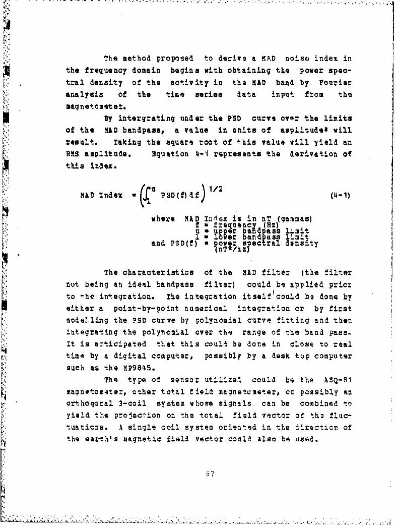
The method proposed to derive a MAD noise index inthe frequency domain begins with obtaining the power spec-

tral density of the activity in the MAD band by Fourier

analysis of the time series lata input from themagnetometer.

By intergrating under the PSO curve ovpr the limitsof the MAD bandpass, a value in units of amplitud,' willresult. Taking the square root of this value will yield anRMS amplitude. Equation 4-1 represents the derivation otthis index.

MAD Index P J SD(f)dff (4-1)

where MAD Ixnrbex is in nT (gammas)"f frzequsncy (Hz)n a upper bandpass .mit

1alower band dass -mand PSD(E)- power s0 eral density

The characteristics of the MAD filter (the filternot being an ideal bandpass filter) could be applied prior"to the integration. The integration itself could ba done byeither a point-by-point numerical integ-ation or by firstmodelling the ?SD curve by polynomial curve fitting and thenintegrating the polynomial over the range of the band pass.It is anticipated that this coul4 bG done in close to realtimo. by a digital computer, possibly by a desk top computer

such as the HP9845.Thq type of sensor ut•ilizea could be the ASQ-81

magnetometer, other total Eield magnetumete:6, or possibly anorthogonal 3-coil system whose signals can be combined toyield the projec-ion on the total field vr.ctor of the flac-tuaticns. A single coil system oriented in the direction of

the ear-th's magnetic field vector could also be used.

67

"& thrve coil system which is used to yield an RMS

ampl.itude is cu.rently in research use at the NavalPostgradnate School,

3. U.mgin 219IR2•UcLtXI

The proposed indices discussed above are intended to

be real time measures of the geomagnetic noise in the HADbandpass. Whether or not such activity can be predic.tedahead of time needs to be looked into.

while there is no model for the background comporoentof geomagnetic noise, worl. has bean done on estimating the

future act.ivi6ty of micropulsations, notably by Fraser-Smithin the case of Pcl pulsetions [Ref. 42, 43]. By extendingthe predict5.on technique for Pcl pulsations to the Pc2, Pc3,and Pui pulsations, the occurrence of geomagnetic amcrop,.,-sition activity in the MAD band might be prelicted.

Combining this prediction with real-tiae solar flare infor-mat ion should give the capability to disseminate real-timaand estimated future HAD indozx values to f.eet users.

:2.

-,4

- . .- 8- , . .

Previous studies have led to the conclusion that thecurrently used geomagnetic indices ace not accurate measuresof geomagnetic noise in the MAD band pass. Experimentalequipment has been utilized, and computer se~ftvare writtenin order to confirm this conclusion, and to develop areplacement means of evaluating MAD geomagnetic noise.

1. EQUIPMENT CONPIGURATI0O

uxperimental equipment, acquired as part of the NavalPostgraduate School geomagnetics reasiarch program, has been

utilized in the effort to develop a usable MAD index. This

equipment is in use in other projects of the geomagneticsresearch group. The sensors and associated equipmnt are setup for remote site operation with system monitoring and dataa. analysis located at the Naval Postrgraduate School.Descriptions of the data collection system and data analysizsystem follow below.

The data acquisition system illustrated in Figure

5.1 r-veals The following major componenats:-coil antenna sensozs (3)

-preamplifi -rs (3)-signal conditioners (amplifiers) (3)

-pulse code modulation system (1)-radio transmitter (1)-radio receiver (1)-insatrumentaticn tape recorder (1)

69

944P1

.1%.

44E-

hnrnrwvi r~c

Figuare 5. 1 Data collection System

70

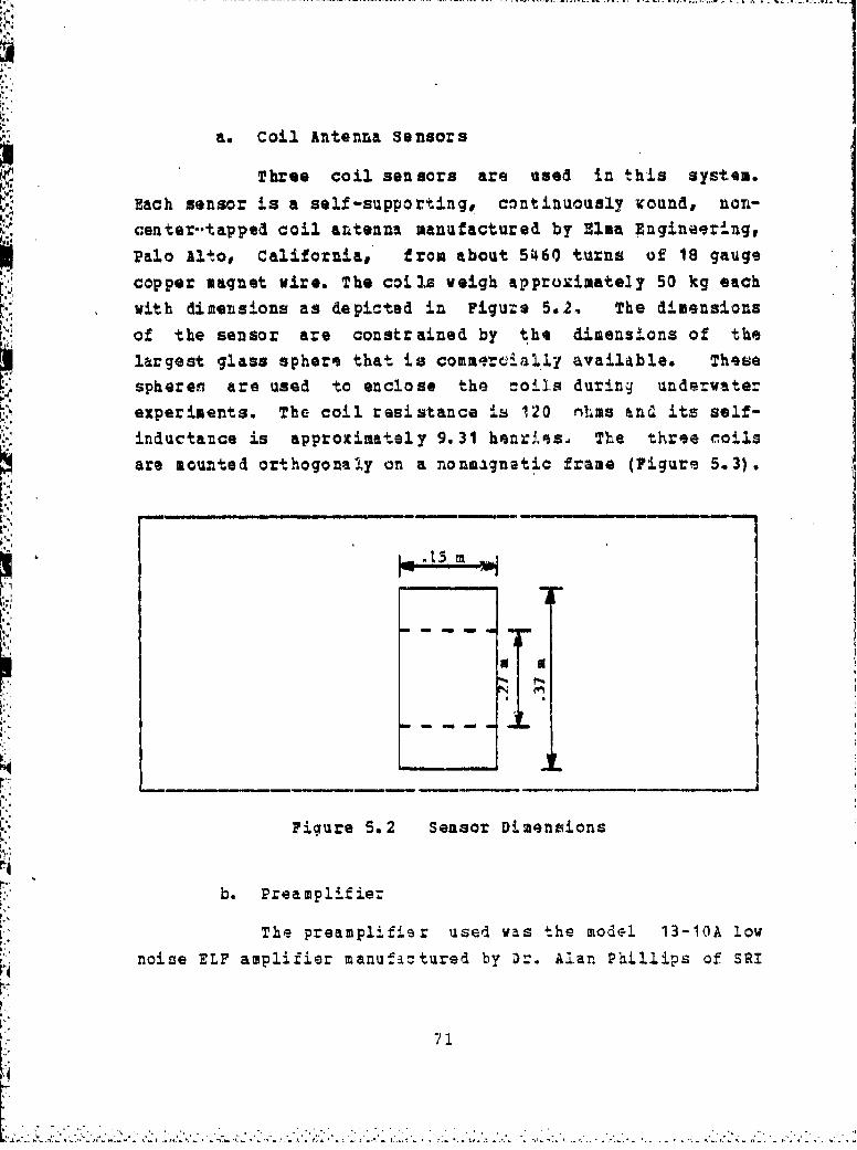
a. Coil Antenra sensors

Three coil sensors are used in this systom.

Each sensor is a self-supporting, continuously wound, non-

center-.tapped coil antenna manufactured by Elsa Engineering,Palo Alto# California# from about 5460 t urns of 18 gauge

copper magnet wire. The coils weigh approximately 50 kg eachwith dimensions as depicted in Figuze 5.2., The dimensions

of the sensor are constrained by the dimensions of thelargest glass sphero that is comm.rc.ialiy available. Thesespheren are used to enclose the coils during underwater

experiments. The coil resistance is 120 nhms tna its self-

inductance is approximately 9.31 henrl.ss. The three coils

are mouated orthogonaly on a nonsignatic frame (Figure 5.3).

- -

L_ .15 M

Figure 5.2 Sensor Dizenvions

b. Preamplifie:

The preamplifier used was the model 13-1OA low

noise ELF amplifier manufactured by Dr. Alan, Phillips of SRI

""I

iIwi

-r U iiiii - H - -

rj

-id

_" _... . .. u-" -... ..

Figure 5.3 Sensor Mounting Block

Inl.erna+ional. The final stage of ths amplifiar contairs an,ative low-pass filter which proviles a sharp cutoff for

frequencies tbove 20 Hz. The overall preamplifier gain for

inputs of less than 2.5 millivolts is 60 dB.

7 2

c. Signal Conditioners

The signal conditioners receive the analog

signals from the coil preamplifiers, amplify them on the

order of 30 4B, and limits signals with peak amplitudes of7.5 volts from entering the pulse cole modulation system.

d. Pulse Code Modulation (PCM) System

The pulse coda modulation system chosen for use

is one designed and manufactured by Dr. Robert Lowe,Lowecom, Inc. The system features 15 channel analog inputcapability and offers selectable sampling rages of 2, 4, 8,16, 32, 64#, and 128 samples per second. By appropriatelyjumpering the analog inpat pins, the sampling rate may beincreased by a factor of 5.

The PCH system incorporates a crystal oscil-lator, and associated CMOS integrated circuitry to develop

the clocking pulses, and a 16 chaanal CMOS analog multi-plexer, a 16 channel, 12 bit CMOS analog to digitalconverter and associated circuitry to provide the pulse

coding. The crystal clock oscillator operating at afrequency of 24.576 kHz produces a square wave output with aloss rate of 1 bit in 106. The clock pulses gate the analogmultiplexer, analog to digital converter and associatedfollow on circuitry that form the pulse code words. The

basic output is a Si-phased pulse coded signal.The data is organized in frames. Each frame is

ehaded by a sync code word which is followod sequentially bythe pulse coded samples from PCM chaanels 1 through 15. Thesync code word i.s a pulse coded digital word with a decimalvalue between 0 and 4095. This word is presslected andhardwired on the circuit board. This ccde wcrd is ess-,ntialto the decoding process.

;i

::7,

-4: :: : : ; 2 ; .• .. , ,: , .S > - .

In the initial operation of this system, a

sampling rate of 32 samples per second was utilized. Onlyone sample per coil per frame was analyzed, making use ofPCH channels 2, 3, and 4 only.

e. Transmission and Recording

After the data has been PCM encoded, it is

transmitted by a VHF radio link back to a receiver located7 at the Naval Postgraduate School, where it is currently

recorded on an instrumentation tape recorder for later* .analysis.

2. 2At aZj

Currently, the recorded PCM data is played back into

a PCH decoder and associated equipment which generates anine-track 800 BPI computer tape containing the decodedsensor data. This computer tape is thban input into the

Naval Postgraduate School IBM 3033 computer for analysis. Itis in the computer software that the sensor system transferfunction is applied, spectral analysis p•rformed, and theMAD index generated.

"B. DATA ANALYSIS SOFTWARE

As was noted earlier, a mainframe computor was utilizedto perform the spectral anilysis. ipply the transfer func-

tion, convert to power spectral density, plot the PSD and

gen-arate the RMS noise amplitude 4AD index (using equation4-1). This program is written in FORTEAN IV and isdiscussed in brief below. A copy of the program can befound in Appendix A.

The main program is divided into sections which performthe following functions:

_ -Data input-Fourier analysis of time series data

7.4

-&pplication of system transfer function-Projection of field components onto total field vector-Data averaging

-Curve fitting aud calculation of MAD index-Calculation and plotting of power spectral density

Data input is accomplished with the aid of a subrou-tine package supplied by Dr. Tim Stanton of the NavalPottgraduate School Department of Oceanography. His subrou-tine (called 'SUBROUTINE RD') serves as a FORTRAN $READ'statement, taking the PCH data off the computer tape andconverting it into integer format with a value between 0 and4095. The data input section of ths main program takes thisinteger value and converts it to a *RAL' number and normal-izes it to represent a voltage value between -5.0 and +5.0volts. This section also sorts the input data matching thePCM channel to the data array representing the appropriatecoil.

The time series data is next converted to the

frequency domain by utilizing a subroutine (called 'FOURT')which performs a Fast Fcurier Transform (FFT). The subrou-

tina. is one available to users at the Naval PostgraduateSchool and utilizes the Cooley-Tukey FIT algorithm. Furtherinformation about this subroutina can be found in theprogram listing in Appendix L.

The next section of code applies the systsm transfer

functions for the three coils to the frequency domain data.

75

The transfer functions are given as straight line segments

which were found by least-squares approximation:. The dataenters this section in amplitude units of volts, and isconverted into nanoTeslas by the transfer function.

Following the application of the systes transferfunction to the coil data, the program next calculates theprojection of this data onto the earth's magnetic fieldvector (total field projection). This is done by firstapplying the local magneti: variation (declination) to theNorth-South (1) and East-West (Y) coil information to deter-mine the horizontal field component. The local magnetic dip(inclination) angle is then used to project the vertical(Z-coil) and horizontal field fluctuations onto the totalfield fluctuation.

The previous program. sections exist inside of ado-loop which enables the analysis oE a long period of datawithout a prohibitive need for storage space. This loopincludes accumulator arrays for each field component and thetotal field projection. The fluctuation data is convertedinto power prior to storage. This is done by taking themagnitude of the fluctuation component, dividing by thenumber of sample points, and then squaring the value. Afterthe program passes through the averaging loop for the lasttime, the arithmetic average is taken for sach frequencypoint cn the arrays. at his stage the power spect.um ismultiplied by the sample period to determine power spectraldensity.

5. ZAfl JIdI Qý Iton

The next section ccmputes the EMS MAD nois- indexpreviously discussed. A polynomial curve fit is porfo'rmed on

76

the total field PCD using an available subroutine (,CHBFT')..

The resulting polynomial is then integrated over the limitsof the various AS2-81 band pass sqttings.

Plots of the power spectral density of each of the

field coaponents and the total fiell projaction ar geneor-

ated in the last section of the program. This is done by

converting the fluctuation power spectral density to deci-bels (dB)-referenced to 1 nanoreml•AR per Hertz. A Versatec

plotting subroutine ('P.LOP') I.s then called to actuallygenerate the plots.

C. INITIAL SYSTEM OPERATION

The NPS MAD index systam was initially placed into oper-

ation with ths coil sensors located in the La Mesa Villagehousing area near the Naval Postgraduate School, Monterey,California. System checkout was accomplish9d in June, 1982.

The fall system was placed into operation on 25 July 19S2and 18 August 1982 in conjunction with similar measurementstaken on the floor of Monterey Bay.

The HAD index output 'and power spectral density plots ofthe ot.al field fluctuation for 25 July 1982, 1237-1406local (2037-2206Z), and 18 August 1982, 0121-0250 local(0921-105OZ) and 0507-0636 local (1307-1I36Z) are shown inTables IX, K, XI, an, Figurs 5.4, 5.5, and 5.6

respectively.

77

- . . ! . ......... ...... . . . . . . . . ..... ........... .. .. Ili/1

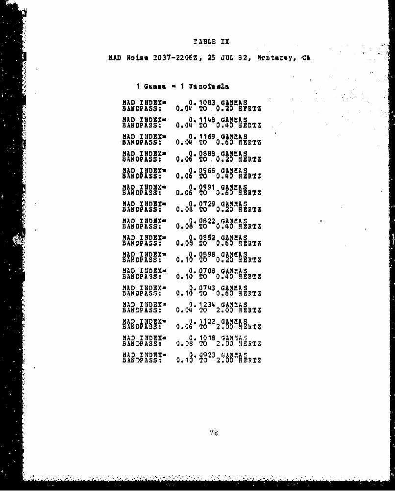
I ABLE IX

MAD Noise 2037-2206Z, 25 JUL 82, Mon'tery, CA

1 Gamma 1 NanoTesla

MAD INDEXu 0. 1083 GAnMuSBANDPASS: 0.04. TO 0.20 HflTZHAD INDEX 0. 1148 GAMP 4 SAN DP ASS:. 0004 TO 0.4U RERTZ

"MAD TVDff, 0. 1169 GAHMM SBANDPASS: 0.41 TO 0.60 hERTZ

MAD INDEX" 0 0888 GARMAS"BANDPASS: 0.02 TO, 0.20 HERTZ

MAD INDIX" 0966 GAMMASBANDPASS: 0.09' TO 0.40 HERTZ

MAD INDEX= . 0.09 GAMMAS-ANDPASS: 0.06 TO 0.60 HMERTZMAD INDEX . .S_0729 GIMM&5BANDPASS: TO 0HET

MAD INDEXw 0. 0822 GAMMA -BANDPASS: 0.08 TO OO HERTZ

HAD INDOX- 0. 0852 GAMMASBANDPASS: 0.08 TO 0.60 HERTZ

*:' MAD INDEXu . 0598 GMMAS"BAFDPASS: 0.19. T;O90? HERTZ

"MAD INDEX- 0. 0708 GAMMASBANDPASS: 0.10 TO 0.40 HERTZ

"MAD INDEX= 1073BANDPASS: 0. TO 0060 , ERTZ

MAD INDEX= 1. 1234 GA5MASBANDPASS: 0.0 TO 2.00 HERTZMAD INDEX Q. 1122 GAMMAS"BANDPASS: 0.06 TO 2.o00AEVTZ

MAD INDEX= 0. 1018 (" AMMA,`'"BANDPASS: 0.08 TO 2.00 'IERTZ

MAD INDEXt 1 0923 %PTBAN TV ASS: O.1 TO 26.6781

•, 78

'"0

r-4

P4

9,r

p.9

Fiur 5.4 P 5JL3v23-20Z aMs ilg,,,, L. . .. . .

9.i

ihA,

"•./"

-. "- ... _ .. . .__. . , :'• ,_ . . __ ' .':_" _ _ - _ _ __'_"_"... " "

TABLE X

HAD Noise 0921-1050Z, 18 AUG 82, donterey, CA

L

, Gamma a I VanoTesla

HAD INDEX= 0.3644 GARK&SBANDP&SS: 0.04 TO 0420 HERTZ

MAD IND3X- 05ANDPLSS:. 0. O j0.0'ui•RTZ

MAD INDEX= 0. 4004 GAN11SBANDPASS: 0.04 TO 0. HERTZ

TANDPASS: 0.0~T 2 .l~T

MAD INDEX 0R.3401 Gt8KASBANDPISS: 0.0 TO 0.40 HERTZ

MAD INDEXo .3453 G&aKASBANDPASS: 0.06TO0,60 HERTZMID TNDEXu 0.2528 0 G201&SB' MDAD S0 .0 O0 ET

MAD I0. 0DEX? 966 GAMA

MAD INDEX, 0. 3025 GAM&SBANDPISS: 0.08 TO 0.60 HIRTZ

HAD INDE•X 02112 G2A1 8BANDPASS: 0.1 TO 0.20 18, TZ

B DNPASS: O. I 0,4 HETZMAD INDEX= 0. 0691 GAMMASSANDPASS: 0.10 T 0.60 HERTZ

MAD INDEXm 0.4047 GARMASBANDPASS: 0.04 TO 2.00 HERTZ

MAD INDEX= 0. 3679 GAgMASBANDPASS: 0.06 TO 2.00 HERTZ

MAD INDEX= 0.3 3339 G?•4MSBANDPASS: 0.08 TO 2. 0 H..RTZ

MAD INDEX= 0.183026 G85MAS3ANDPASS: TO 2. HERTZ

30

- .� 9II

.. J,

I0

'a

=

r

.4 0

U.

U,

6',

�oaOi-4

p.0�

I.

I.0

U,'I

I-'

0

I

o o 0 C 0 0-.0 C�J CN to

� �LtJ �r �) �13uIoaa'

Figure 5.5 PSD 18 AUG L�2, 0921-1050Z, La fl�sa Vi2.lage

82.

T ABLE XI

MAD) Noise 1307-1436Z, 18 AUG 82, Monterey, CA

I Gamma - 1 ManoTesla

MAD INDEls 0. 3188 GAMMASBANIDP&SS: 0.04 TO 0.20 HERTZ

MAD INDEX= 0. 3246 G8MILSBANDPASS: 0.04 TO 0.20 HERTZ

MAD INDEX* 0. 3267 GAMMASBANDPASS: 0.04 TO 0.60 RBRTZ

MAD INDEXu 0. 2297 GAMMASBaNDPASS: 0.06 TO 0.20 HERTZ

MAD INDEX= 0. 2376 GAMMAS,.ANDPASS: 0.06 TO 0.40 HERTZ

MAD INDEX= 0. 2405 GAMMASBANDPASS: 0.06 T2O 0.0 HMERTZ

MAD INDEX= 0. 1585 GAMMASBANDPkES: 0.08 TO 0.20 HERTZ

MAD INDEX= Q.t985 MASBANDPASS: 0.09 18o 94 RTZ

.MAD TNDEX= 0. 1738 GAMMASBANDPASS: 0.08 TO 0.60 ,IERTZ

H'AD IIDEXz 0. 1031 GAMMASBAND)PASS: 0.10 TO 0.20 HERTZ

MAD INDEX= Q. 1199 GAMMASBANDPASS: 0 TO HERTZ

MAD INDEX= 0. 1254 GAMMASBANDPASS: 0.10 TO 0.60 HEIRTZ

MAD INDEX= 0. 3504 GAMMAS3ANDPASS: 0.04 TO 2.00 HERTZ

MAD 1l7DEX- 3. 3137 GAMMAS-"NDPASS: 0.06 TO 2.00 HERTZ

'MAD INDEX- 0. 2801 GAMMAS"--A�ANDPASS: 0.0 TO 2.03 HErZ

MXD INDEX= 0. 2495 GAl,',%SBANDPASS" 0.10 TO 2.00 9?RTZ

32

its+

=E-4 m<

W C6

+C W r4I

C% L

-,

Figur 5.6 PSD 18 kUG 82v 1307-1436Z, La Mesa Village

"83

SVI. r2o_! ANDIXo§AZIDATIOU

A. CONCLUSION

Analysis of available information regarding current

geomagnetic indices and the actual level of geomagneticnoise in the H&D bandpass indicates that the currently usedindices, the K and Ap indices, are not valid for MAD opera-tions. It is therefore desirable to derive a new indexwhich more accurately represents thq geomagnetic noise atfrequencies of interest in HAD operations.

B. RICOBSENDATIONS

A tentative index was developed,, teshed,, and sample dataobtained. The data analysis for the preliminary system wasaccomplished using a mal.nframe computer. It is recommendedthat further work include improving the index and thesetting up of a system to on-line decode the incoming data,and utilizing a desk top computer such as the HP9845 toenable real time dete minat- on of the MAD noise index.

The spatial coherence of MAD geomagnetic noise shouldalso be investigated, with pozsible application to noisecancella.ion. Additionally, the fsasibility of the priorestimation of geomagnetic noise should bg evaluatsd,possibly by using the prediction methos proposed byFriser-Smith [Ref. 42, 43].

84

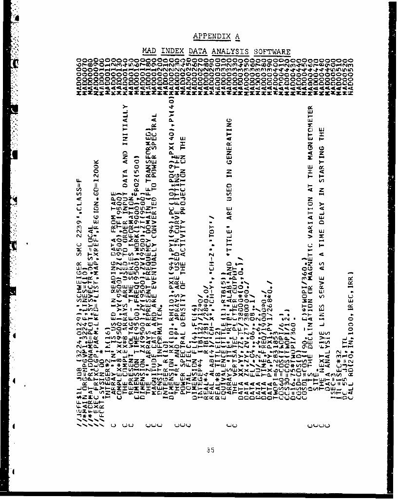
APPENDIX A

MAD INDEX DATA ANALYSIS SOFTWARE

0000000000000000000000000000000oo0000

0000000000000000000o000o0o000C) U.

< 01. -.L

0 1 . zf - -L% a.MQ

11 11 0 a M

V) 0 L0- .wu0 Q W-1 Zu-L o-

_j z Cru .-Q -. uoLLLC, " 1- cr.bLL 16 J C6 I -

0 ý 010-< 01-> z0A awwmsý4W -Ze.) "

U.N.0 1-'-'n4 0fDC1 L-.1

Ll~ 1 0 -CCU>- 0.oqo2: 11 CL Q0%C M~2_ CL L)

V1 x * l ý.( 0-w- 0 0-i* -$-0Oj--4cc 0.W . I

oc LUj( Or~~a'-> -o)L-n < Zr4..NW- LI%.00)*.0 0'- Lo LU<U

LU LL ý 4%0~~ -0 > Ix L- t-0. %%3 11 wJLL I-C -'LCY016-J) M-.-C -C1-0b4: xb=01I.1.1 MMW u..j 0. . Of I%- 0 -. L)aV) 2p_ V L -C.4fl0.n. 0>1- No m< r)O* o- 4m

oJ) WO. Z Zv)W -4 CC - a *2O (VL U- -ZU 0 W -waOý. C-z r4- f-U C *0C-V z

as LL. t:k W-iWWO-U 6 -q LL 16~ r4 -

OMc~ 11 x i A0%W u..W >- .440UJ 4 .-. '4.4 wt 0 .. 0r'ZuNCCL. LU _-t *LJqt LL0LUr-4- 0.40X00 b- OU> 0-c4(0 t- .

-0O ON MCZI . 0 XZ -iLO14 -t('~ - .4" o -> $LL.CLNt/ ý- (A *i Z *W1CLM' Z~m*Z.,C-) -ý C- V) %)C Atf-LI Q 0' w(' e. w ~ rC'f- 4 Un

4 N. 0 If WX U>UL)J(At 4Z 0c..10 I 111)C11- 1N1'.1 *-. .<(no-m*n l IQCL v0..4)% WOZ > c 2 -00 .Z W<Z*--- . P" cc) -10 "'.0'% LJ > ~- du

N,4*ZXU0. - U. W r b. CZ m"=x Mu Q0 Q *L0.4 Q' 'J) .UNb- (.*'-. - L'1N - ~ -- W - ' L. -- C- J(.

OCO..00ZZ 0 L .<ZtU4Z -- a*0N .. (ZWXt0z-CL * 2 U 0.UC fLL* 4-UL ,C(A1 ~

Z U a ( N '' -. - ~ U~

C000o0000000000000 a OOeOGOOC) (ooca Coooo00000040000%ti %O-O I#~ nklnQrm ov4~- n.r QaOO ~~%O Ca P t~u o-OO P0 c 0a c0c oQc ooa08

444 444< 1Ldw4 4 444C94 C 441444 444

2: C) <= 0. IL

detOL WQ soa >-OCO-.. cU' 1C.0

0.4 w l . .C

I- 'U. cc >~ I )I WL

Z" I. UW.%lU.I 4 IU

LUO ~ ~ 4 -a, xý

0000000000000000000000000000 000 00000

000000 0NNNNNZero~

IAý 4:LCr~Z2Z Z~ Zr1ZzI

z ~~~ -j )u

Ul. i-. z .

z~iQ I- I

ZO

0z- =4ý -

w~~~ C) I-L ' ~ p4Q U ~

- UJ ** )'-C.)0 4z %t0~ %a~gI

- , aczwýI V) LL CO 4 (z aa. 01 ~ 0 C 0O a r0 a

@"I '~ II Lif-(Mt1U. C. ONýD C* *u LL *** .a* * .-4* LL LLW UA . 4~U I", I-IUlCMN I-O -NN%r Jpt.4\J~ 1-JP"N* *a. ~ . ~ -- o~u!.-4t Oi %0 C,- OMN0 '00"'4Q *IP-MO r

CeMCZ2!4 LL. ( * CD a (r P- 0, 0 * c

V) LL)).0 ;> ZN 4c ON u".~" .

11 11 LLLL4 (0MX 4%2 Ok-0.jx( .J(>IN JW, ..J)')N .j x >-NJ ~JX-N X"I-z = OCIi~% W01L *XOD OXP*O $X)INC *X>-400' *X:O-NCO .*-NCOXt'-

L0ZW* WM-L I- .. -lj -ill ZL Zj .. -J-U -. 1-4 -J.- LI-..

37

LU z K~~dgZ Z2 Z Z ZZ Z Z

CL Z

> U 1-4 0W

1-00ZZ39U,00 "04 L)Ll.N00. LU.IJ

mo--I 04o00z >Wl

02

~ z~U~w I- U.1PI1.403 -0 "Col. 0JLL

t uj~J U'C.I" ,-0LL+ t.NW CLLL> )j

o =-j cl,- L-c w-a

'r II IxI OUJ = W

- >o- II-uJ *** >0/ I4-W Wt Zz I- U.u. J V)-40' 1- ýd wv (3 U.L.L o C-

- ZWWCU. r-.r4.-4w4 e acW14 N

".--CI-c -- w 4^

Z< LLW >-NU.L. .4O)z LLU

+ 0.0N X t/LO~~) C4W 94 W-.J(

0 -j Lu Cz~ 0~ I= -I-

+ + 1 1- *** III j.j-It

XI

x ZQ 0 11X)>Il- ..j>- *II)O->l-- I-.W MU4~~.N P'.qL.4.i41 I.Iu(U4 ZWZO 1w1j, . w 11 IIg 0g -. co 111- U.,L If .J II 0

Wso-~ it it 11 11 =Zi "I-" it 1 If 11 =)W;zo-~--:) - -0 ' "C0-04 2ZIIZZ=fI- C= NNZU W -~ Z j'Z ~I-4,- 1 UZ- 49~O > ~ f I I - U.1.4 4 '~

ONNW C. --144 QMWTLQM4QXX

I9V,' C' C'h

WU(JWUa

40

W..

xx

o..

I! _L

Q. C,1%%LLbQ

I- O CF-9. . 64-

m 111 L. P-- P4 .ý

0V&Cmr.w .-JIL 0'CMV

.* V-4(N U%%r r- U. 0 Q. m0.

0.. 81.3 -

Coc0c 0 cc00cc00 cc00 00000000000 00a00a0000cc

(Y 1.1.1

W~. 41 < wc

uJW CD>2

L.I.1~ W9

0 1-m = .s

qe. Iz 4W; C I

*ýL i w2C 0 W 0~

U611X>->- Ia ay -i a

ýýe~I u- 41. 1t~~% c + zuý--ut ~ - I-. A

Ba 000 "= , jF

O~u'W I- I- - I-ICWZ44 0 W(.D -I.. MC-m -m- MI

x a aaa ~ ~ qQ

+A*O* (L It 11I it 11 Z )4I--~ .i i UUJCaý If it CL'.41%(dNN M4 fqlý4m4 .4~

OC-X I- 000 -J4 -

xc x xm- OP4g.4u'l U. Ill ZZ C -' -U-U- %QZ.JV u f(LC .~-~.a

X)( .J 0~0 I 4 W-4LL..0Zp~a~ C~wNWC)U.I ~ 0~0~04

000000000000000000000O0000000

ocN '4.

I- -

U. L9

w o wu

"=w 9 W

cz i' W 11

fA >- _j 4.0OJq )V) W*4W

U4 ~0LJ LLW

CZi -- c M.Coo w -l 000

mw, Q;"-w,5 *- a.I *4 ftw-w ~WO LII. Az ýcW a

4 * 11 c ..J .1W'4Ud Uf 0 -0 o-o

4 V-005W4WW -;> R-*-0 o N 11 a0w 04 0100 W- w

in -.- No W404f 04L-@

zz 0 L WS.4=0 ...J'J ý 0" v ~ +' 0 '+

CC.W LL =WOOD ww 4.4WLU J= wg- z 1 be .....c ".. -D- N ý U-L... W)ocr~., M 0U S" r so-J O4/)2 0-4s-o o+% Vl-CJ-" 42. 0 - l U 30 Wo.- +. II~ X<~ I-'ý-e = I4,

X.Uj 41 Q 11 0~/ -0 -4- if o-L. I-xw wo~-m u < ) 1V)U 0y 00-4 *12 ".')-.o 11 4

-o 56 Y. U e w Ma A l x4 1ýZ.1z -6- 64 0~Cc~ -4 0-kLCLLj06A w1Ii=X = = C VUWA

Pw l* - - IM /)4.SL# .. U tdý-4ULU ,-.*-

OLLJ- ~N W4- 0 * -- ' A

0 ~ NI-A~ ~ cJ- rV -- c~-'0~~Zr f*n4.1. C&. U.~% 0e 4 . U% &A414 % 0e'40 0 * *

I-g o 4 1146 O g "ct ,tý c

OOOOOOOCOOOOOOOm ro0mm mO oOOioO0OoiooeOcoOO riO

"4:

UU

U.

-w *

ca %- U.L

W N LL

P4 t- < 4* X (T-4m- -j c

cxý6LUM LL~j In 0. C a3L Ity 00U>. QzZ "0

14U " 4n a,0 WW,~ ~ ~ uju z04W=CL

(A 0 >- UA fyLt-. -0 - 0(-0 I.- - W

.0o LU 0 -. N 0 oz c IO"4PAmix0. ...JL.NP N 0L c L)Vý W. U 1 00 "

-J 0.4 _j ow~zZ emI -62 MLw .0 ) + LUC LU. ~ LU 4, Z - Lb4 "I- aL' LL VI P

j Oa % fo 0 ' )M c a.. u)L II( =t&' W-. WO.-4 4.4 u-aixf. z -I --Z mCa.--4 ý-VO - j w

U.U

LUýV%0 *- (/ ~ -

00c 00000000 0088000 0

>6 LU ce.Lo -j

Atixc 4c .. 0 4C117W 2I.U= CCý-C).. ce Lu LL. lo Q w

>ZO COCO~ 4 U.L 2 ZII- (Az ZCI. Z11D 4 W ~ U

VU.W W40cV) WU lCC zI

0 z mml- CD1L)cr LIM 021P4 LL I-)

W < V - 4oW~OW J -a. L o- Z 40 XU.LWh Z

C)ZWi 4 OIC ~-Zo II- = a- 0Z~~~O II (f) / >4 ýU.II- z

Old~ C4 a ce - C*Wujw u~4 .- z .

a C- 3c W4 x 0W- Z LLW I-i-d= (Y cc-C W Ctzz LI.4a.wC..j UJLj WI-. 44)( OX X4 C.)u.0 C= OCL WWZ99=66 =m CL cW tI- U. 5.UI-.W W WU

otCbV W9~ )- -jI-ZWICLLO2 "4 * LI. 04 1-0 (D qC4z49-4C

L2)III% 'm ZMI4 Z zw W. j4~Z)-Q.-.- 0 =Z * 0. - -~/g''Z~

CL4.' o.3EC z ZI( LL tI- k-ZU.UJ 3 D 4

1-h2UJIC,4 WUZ(A z COW Z =~ CCUh-.0 0. WozoI.f2-4Z A) LU CCI- VZ 39 4401-- LU Z 0 #0

uikW *z0I- Z02 * 41) "CzczW 0 0) >. teCWZ=4 I.-0 V)C)(44L~C Wu. >-"- 0 cl I- Q. "4 ZLO94- 4WL4%v-I--

mm 1-1-420 0.W-O) ' Z I 0"' ow) 42LL.=U. z U l-~ WV WWCC 0 WU -. 4 )ICIh-* C.=0.CC Z X I-C)ZLI. 4c W C 0 4u. W

44.. -.JW4 ce X. (..LLOCC 41.. X> =1)

OW41C011N4 z W xW4 -OC-a C= 20.- W.4)MZ CJc4

m LL2Xx -I-Cz z i-U. * (nu. 02 W oz wIap~1- Oct 11 20 ;0 O -0 WU 41 I xz Z cc 0- cc~zz Lu 22C

U. U.)p- U.-O pi UU)V41J M 0) ~ LWA." ui 6 LU Q(LU 0 -40011 C-Z-4 C7 -w~ X Je<C * LULn (JOC)O-6-40 Z...Jcu.

Lu LLA<4ý- P Lui W I- u 0.0-IZ UJ4 19 Cl- Wil-4AiflUi JLL~.2 ZII-4 .'- w :0 &fl XC- Cc 4 11-1- x2 Z II- C.-iI-"b. =W0C.~~-.W :D I~cuiO Z-1 =W ZVI (m 2m U.

c a CUWi-ZMWI 11 >V -0z

Zrv C. W k" W4..J1 -j I

4d

+ +

(.40.4 >-- uj ujc 901 u- ZC.ZI ZOO.%*ZZM..J .41 SLL I ~ F-. w Wý- 1 * C

c.Z Gee 1% 1 0ý *Zc0- Z40.0~ 400i I.-At O

PUACW X.F-* 4b-46 z-I 44F-to1Z3M-4- 4CLUBIF- U..ýZ N . ,* id Zoomi

'* - ..J OIL 4CgotZ J01E Z*wmlK ZO(j C.7 7b-' P4M4LJZL2 ..J 0-iN"-LLO' 06*coxL

Q U.ZZ CM I~ tW LW-n 0 4 LU V) Txu4-0- X X= 11I 01 zr O l-JJ O

se Ae ix *) in ec44CO.=ý- 4t ZLU.rNZ*UMO 4rm(Y ~ O M 2mce o -ZU. : i Z F-C; .ZM(AfLLE

coq31-W Wjo ") ý-)o m 0 ZXI-'4)" 4 =0. Z)P01W 4W C

3 O N S 0 0 4" C.JWUJZLW4IdILL. -- V wV + C Q C LLUJ 4M

ce V) - 0.i4m P4a 0 - .o.= LIJZ cO- 6 o~u:z4.. E

U. 0. V) CX -. 0 0 % I JII- UWZI-Q 4LIj j. 6-z~vz co oW. - W 0 W.UZ N * x4U. -Jo 4QWLtF-= ~Q.U* 0, 0~ ý-2-

*040uwW 0.4.44o. n ý*zj C.F-c zcgZu ZZXO Ig-U.-"N,( Z OXO W..JZZL)*M4 MU.1 "C oun4ov4-+Z .EtU.J)O* LIN04.J.W) CA :L C. uca0 ji.-O

.7 CL J,%o.'' I W3J- -t .~ * Lg I- II UJ X.J.QJ )'- wi *m. * U W .. ~~in o4..) - It0 .'B

<-4 ~ -F =w Wj*.o.* 4AZ P'-4 AW01/iW C. LU ý- 4* U.J Ot *'Aow

crWLJ4 4. * 1.o Z-*'A oz WU. uý of* LL.jQC*U F-Moc OX4'

(9U--4W,-'Q*X J* U~Ar2ZQU L.Z I- QN3I--tA M3Z- 01--- *-tAXM -4LEI 44Z44OO-U) 3Z wO~e 2 2 CF- Z11

01 C .. .404 zII 4U -i* I a-~~ .- 'W Q OZ 6* UJU'4* 0

.(e. r. zL. 04 *0 4 00 Z4ZLJOZ Q4;In e t .I -U.1

.1cc 0- g m4 6.4 Z W'(~ X>4WL'- C~ I- - 0eC-KO X =-h/)L0 ie .jY On WLU-'7 .W Z-AU Z OIA' ý') +1 IoilC40 -I4% X F-L OLuI 44z*4(.ccQ ZJZI1 I-.. 'w4- I-- L ZLV)-

_j ,4 = I 400-' >* '-=4> Zc..jc zI-ZN Ji 1 "4* >.o *

zA 4=~-W e ~ I 3c ~ 4~ RV1AC 3ZU~F '-012 dt00 --L > LUj c. M IdA

Z= v.4V) 0 00 .JF-"Or 0 1 -V) v)..i -Q0 0 ..I-I W O z-447 4UIw Z0ý1 W *4jj Q(v-0Q . .4 ' .4- V)wFO I..44U'

4RC 1. 4-Z.'I/) a IA gt.- Z ~W iC.*~ Mv-U.I/) ý- L% WOA47 UJ*O-Z% :W 4t~r--c v P- (X 4fw 21*Fbm-ozz 0W.4 LLJXI.U cvl-c ~ uw vl 6-4 X

VE 1 44 40(N 3J 4* '0 Z .j" I-C ..- <LZF-400 I-J~ n d,'LZ ~ ~ ~ 4 4- §..b-fl3W~ Lwo &" 1-j q.-'m ) L 114 F -F .)(d I- N i '.4-oXI mo 4. Z ~0 40"~2Z6gwO 21-=4 40U*UC OIz*

"IJ IV W WX m.ILL.LL I m" W.~ CWLUZL ~ Z4-*Q.0F ZWOQ.3 " i zm- .- C 0. U..IJ COO F-4IJ>-...-' w--F 'MI L..) -l<

I II"m wo-0U..1tma >X> L=U-40iz-m -r

w aqcou VM -Z -IL co--C Q.-dv -. ýO -4 '

O000000000NNNN 888No OQ

LU~~~~ L)U1 l zI o w4

4 wtl W4 .0 x al bLL -*4

z L 2 OUIbm Li 4 OW 4 Of l'- <V) Zt LU. 0*10 m wzU.0 .. MCA TIP- 2-Z I .. I-Lf1owO

I-. MIWh 4U' O(Z. d4C 11~- CL Q I-Zixo-4J..j#A V) V)LLI.W0@j s Q. Gu vtuWu0 C6 j. L1 P-q z< a) U.

z z =0 - IflI 0 ti-- 1'. == WO W-.4 ýJJ- o w 2

I-.4 mC"~I um I0..J. *"4ZL O ~ u.* .W0AC 1-AZI-tzo. 4 ZA0I-=oz.to ' 4 w~0 4 g

OC19LUr . ZI CaJ to~ UIW .W (-4 .Z)f -> Ial -. L)4L ~ *( ZZWW*MI.40 -= ozL4 I-&WJ

2 '.I0..40 04 40AW4 >6- .Jw Z w oLU~~~~i =0 a) .- LU 4 wI-6r 00 0.

w L w2oi -Iwl0 (n j~2 I00041616 U.1 cU 4c0_c d J *

Z w zLUzw I-a. ct m. mci- 4u-dw- 0-4 m = -10 *I-- = oco1m cm: =CZ XWWMWX 2-OxLJ42 -x z

f,- MAJ%.00.U.. mI" Ot0C*WWUM.Wo ri-i I F- a U~isIA -W4-u.zo MQ L.) ...J u.zw).- I 0"=s w =N.-

lUI C 9L ~.0.0 LUZ >I WOL0W=T "2*L& OP o 0S2 Ill t/*W 0 Uu...jmz4 00O W~ 2 A "wý-X c 4 U..>Lfl

q., ~ ~ 4 =W NxWW aU. *4 1043Ce (Ye >-A 14 O D

-- i~soO C-Wg~ or cf.' 4AO. C LU 3

0 4 I-oJI- (.lu4 S40 I0-20 491--4 <. jW, z LAW-IA 41- 0>= -9tIA1fl

A =U.j 0.4 'C"D .. /4 U0-'0 ~ C - 0 A Z

z ZWO-..4 ý- ~LU 0 4w - zL-J2-="W't~9o~ - ~.I-I-A 2 L0..)Z~V2'-2 1Q.LItfl.~I- 1- qiGW. SLtt~4~ '-,Luc: wL)ax.J-4 0/ W4 4 . Q IW Wju

LL)C 2 oo- C"- IWI~~-ul0 U4 41 WXN -jLU 0w. 0 Q 0.1/ w I ý -4!9 - I - IAI-= No Wv I m e

w~~~I-- ZUiz- 2QA X)U W -0ý wz -Z 040 ot 's LL W 4U 4

LU~~~~ ~ ~ ~ ~ .- I uJI.J4 . lW- 9 U. L Oi Cw C uw Z=LM) an m~o,..-Z a= M W CDL .03X I- I

0 w < 2U.., zr. a. -U.4xw)-0Zx WJJ== i--W I cLCl- lbNltm~nLi. u-~0i 4UJLUWM Z- Wx" (lu. 10 .11 aNmN,4t4

0- I C'l-W-iz-Q <m 61 ZU4mW2-00 0 -ý-26=)Lu "z1 114 ZXOC7Mwc= 44 LJV<Qo& =Z -W=0004 W44 Jwv~wIAUny-'

44 U.o 0IZ W .00 0-0 2. Il 4-t . Zm<u.t*)4AI- Wo =*X3z L U4/.x3.-U.-

= 4 0 4 * iX.Z 0L-U'4LlWuxoa 0 .wl- 4CLý.., ww x~~4 lc1-0.- 4 N 0) Q'J. U. 3~1/1.3lU.U. - L WWL#- OCQ 0

MM00 .0.00000 0000, con c c c l;O c

a V

.j X4V) 0.4 x <z

U.i-

Li. ~V"

V) (7% 3r I-

Zj 0. at

I-. 4- M -0.w 4 X0.

= 0 m

ý4 2: LL -. z

- zC) ZLL 0<-. 7--

0 ZTL-o. U.c 0 LI ZLi *,Z z

,,4 -- 4 0LW z-r ZL..1-U-4 Zl- 0ZO~~Q

0) WZ ZP-4 wI m<~ Nr "4 cu VZLe..W Z0- .

*Z ml, U-i-.% 4-.QO. ON C- 6-" ILt N CL~- --4 Z -. J ui t -4 rn - X - 4 C -0C

IM LUC- -d4~ X(1< X- ý 00 WJ z 0 LL)..)C~

c-~.< - I- cl4- 04 0\ ON'-. V 0">Li .u4< WJ do .LUW)-L W.~O .9ý (j Z Wi 11 Lý m

4 * 411 11 1' cc >-0 Z - Wj 4- - 11 X* J.4 C.) . Q "(X N~.?Z L& J O W"0< ZZO..."4 X'-4. a. C2ZZN Z ne J-

C Lu O11 t0 0 V. 7- t-Z t-'.3T 0-1,- 0 0- 0. XI~'p.Iu.- .. iZI)'-'4NU. 4 < -04U. W -- N.w -j ap0"M4 4 Z Nil =LIZ +

0.. ý- Z w zC Z all 21i l\J4zi 11 It -i1CYCAIt -- LL=-j =DO(\l<44.j 0 C3.O= tww<ZI-NIZi- z IQlz 2_.j <Zx C-i-... 0 xeý-ý-c -0 ý-4 .-I =N- M11

LiW-JC0Q0L Q. 06f%0~0 0Q~-ZO*Z X Z0CZ- 6-

p.4 (J l 14 l-

LJj~

coo co000006=100001=700000eco0000 C oo000o00cuo00e0C

I I 0<> .0U .0 o

Uz~i 0 X A<

LL z 0 WIC )

X e- ZN39 0I-M LULLJ ". 0LL

-- Z Z Z~xx. 0 O) C) >..-

U.. CL- = *Z'I.LI uJ

CIA 1- 0 l' 'j

wX 1`N a v-4 P-4<WJC.)

w Lt-- wl'-LL We-

0 0. XWZU.

trl c j -L al -.) -- Z~. C-

< Qý 0 V)4~ - I-T LonX V > L-n" W -*Ii rZW+ - 0 IIU.JZZ-Z W~ 0 o- I~itI M (M U

U >Z0I2.U UU.. IA *~s..Z.-Q Uw LL.LU -4(l)...U...Ll-Iý- >C "p- N-- -Z 1 Ccz v-ý 1,- - --V -f- - -dh

0-0 1-'(J 00 % 0 0 r- F-4 .Z

0 LL%ý0-4- U. ~ ~ 0) o- .L) I ULL QLU Uj a U a U Cl U:CL1 Cý-42 1 ~x*0f-4mnmp-4rs-f-" C 7 :.x Z : rnZ 0-t

m)11isZ LU +C 1 .1z i 1 1 WC 1 1 1 1 371

00000000 0 c MC acon00 cc a co C0000000000c00000

-JLU LU

u~z z

#-4

N 3 LU

0- LL 1 N- *\

IAL it I0~ - -

W. 0 N -1- - 4 0 )- NII ~-4

t= .4 7.I" -CS- I 0~-4 +N 4

' ~ ~ V 6.~ ~ .. IIZI . I4~J4' 4 -0 II N -jI 4~~~.011 lii4 11, It. CZ 44-++ r. - Ul4 -I.NI- 'CLU ZZ N" 0rFNcLL 0. mN O n N

cm ZP- 1J4 -L ft cM4<=LL LA ft z . ~ -.0Nt1- ll-"C4- 0-4 0-4- -r i - iP- -4 0 - -4 -cLq<

I L I .4 z Q.%% IIN IfL It 0 Il r~n 11 ..C21 UA

(i- 0 0 ,- (N N -+ - N4m.P i 4 U-ý C m ~ ("1 1W- -d if 0 0.1 <- -+ r-4 4 -W1Fim 1-N

Nl- I,- w c I- 4 Cr i 4 0 L- L () )to .+ C

CLz I LU 391 s-i LU) 1 1 z-J 11 0 :3CO404 -37

Z 11 0 -IN - tO I- . 01 1 N IXC L % -- CU- CD-.- 1 LL

4 O-N -MQf- P4 M4LO- O-N -U C' %O-N t

%0%0OO%0%QOOOQOO%0O%0O%0 %0O0OzOOOQ %0OQQOOOOOO

U. t-

LU

~~U. ZN~ ~~ ~~ U. 1 '-- '.4

I.-. *

i-I3LI" 1

0. L

U. L LJ .199

OCOOOOOOOOOOOOOcc C cc ccOOOOOocOOOOOOCaOOL)

r-0

X -0 A-"

mm+ x

X 0 0-C :: 2,. . + -+ ý4+ + 4.)

1 + -4. 26 ) -.- r_ M N1 - 4,_ r-(4 I-t r4 1f

**c -4 1 1r4. -o Q4 0.-4.'.?a 4

t.Lx 0C - b- -- -I * 4+ 1.*.-4*

10'4.q NT %r v, -i U

00000~~~~0 ~0 000 m00 aso 00~ coo000200

Li)

,U.

4 0.P-4

-lu. N

wiz

0. -e't0 0 %0

0 0*-4 U..I-

0- 'ALIJ- -up*-4U)O %0 LL 00.-0 - O0.-N

W - -. Mttn .J - I*jL Q. LL. O.U.-Q*tN Ij*4+ 0.4. omm T.i~r LLU%6

ýCý=L%=~~~~ -0 t.- L 4 LXo- -4%)0 -- L. M,\iIt -4 PC u-jr U--jCL - u> *11 I J 4 -oz

1 .4 M - . 3* 0 wu ".4N-X U V. 2 JUi - " Lul")4.. 0.c.N

-~< -Q'W Q6+ "*W( 11 -+ uuo -r- 1 -1 -4LUh0 x- "W0 c0 0.)4M0 0.0 z. W Z .4w- 1 r~m3z o/Z ++N

N * =< (-D .4 1 l ýr ILJW X~-)IJM o w) -Zzux" 1(.I0 l.0.

4 .w ZF 3

0 0'. 0n 0 u~ COU'icN ill 00 r- -W

u% ~ ~~ ~ ~ '.J 1)% L1 Ul A

P4

C Ia -. U- LLIN U. I 0.4" ýU

I N- - t+.I t -t- 4Mt I N. Z. P-4 U. 0- 4. .

00.4z -. 0.4 OW L t t-, + -4 z I' -4 1, -5 " 11 0 XZ * m- 4 I..1 % X CL %% 0. L'U4 S-Z IN p . :D

I.4I "O I4.~. m~4-(N ,~~ "lr -'f P-00+ -*1- ev4c )C14 0 1-*a. wI--4 Z ý,- M 0'. X.4 'f "I ý) +-0- -4C ) .03V)-t ý

11CI i " 1 2 1 -411It111 U IUJ, ý 11 0 110 1 O-'ln-Z' I ~ I- if XaM - 1i L1 -11-N.~I 9 It It "0.~ S 11 11 -- a" 11' 11C.daIt"1

~ I -wo0-4 ton-J= - -J 1

2wwmm WWOM O

OucucoOOoocOOOOOOoOOOOOOOOoOOOOOOaOccOOccOO

p..

z

CLC

00 wo "I- p (Ar- I LW+ u.I % "V ft dr C-4 dr, "

aO lom t+W+ CN V -" art ." % ~

I- 9-. 3Z 00LIVm .- 0+l O..IC WL U11 N 0. 04.1

00 ZOu cl- 4- a. r--j%. Wt o aI'p ~ ov U I.. "f Q ~ U - ~r

4iIVI vwr 1,Z CO I- CD 0- M'-trN *IL J C\A*UI W 3 0 Q M3 .* N( * -U.. 0 - I. 0vC 9L 411- (

r)-tacr4o.,r~ z i z1 W.I t&% 9- 00.4m iC- U. 3 MrrCJ .

00 a 0 LA i 0 2%nNO u W4 10 Cc C-'-4

0 000 a C~OUQOOcoo Im co 0 0 cc 0 QQ cc aOOO0=OO

K.0 -4.

z

zNILL

0 (4

O N I- N LL-. Q- -.0 1)

Z zu )Q=, - ,uJL QQ I=)Q. C.4 %Sr4 .0.. .-4 F- I +- <U

V)14 . 0c"LL n-0 UN

MCL'Z' lz a -4 Z -.04 0- ... U %

4f- dN ~V 4 Z. t- t'J X Ln - XCI-t-0 z. rz e- V I= )

It ~ ~ ~ ~ ~ ~ I 11 11 C4".OZ1 105w ým z1 4 1 -0-NN I -wI -Nc'4 I-I -.jm

XX 1II 04-4 1 1 I.L < - 11 1 I n oja C

t~ ~j 0 LfQ W~~J(~W~rfl'.T '4- In C o- ?

1," 4

a o0a 00 00 0000000C000000000 0000000 coo0000000 0000000

c Q0 00 0o Coc 00000 a00 CZ000C

LU LU

ccc~

.4xz .ui cz'qq~4f .- ~eLUirol6.3 -

UJ0 U Co . a c

WU* C)uL.

LL*)-' - W(.'- 0-

WM-~ .Z0L) -

0d cr. LU(Lfl0-I lCOL'LU 0-W*VACi @LLO" > C4 *Go

a~.u. f-mp- W V

z 4C+CDQ.0.4 6..j2=w 3: WV)o ~LUQ~ -0 - WV)LV'..2W)

S0 < 4 ~ ý; X'0% <QNZ ) N --- - (I~4 ..) C 0 * -

OD 0 .d b.. LU-=1-4 1-Tr 0ý >S A~ +4 A 4. tj IM X Za.cx U. U..

dc n4 .4 0) .4 =-647 o -orxn- ~0 7f - 2: LU Wc- cý, XQ

,.Z I .(.ON-4 ONOJ Z--< 2;:! < c x ~ r.< of - *c) U.. P'--4 S(NjI'h I Q.0L2.Ul 0.4.qd '-4c; 4"~W~/ I"WX4 (1] I-.Qv

z 11isI11-10.4+'-0'-+ 4II 04411 u ~ w :o- i..JW I CC U "Iln N z 110110 JIM LM Z Z Z *u.JW:C=

f.D-Ml4+ + -;.41 - 11 P4 11ll- -I .j- .,w->4- -- » WUjt ..j 0Z b- NN*14Z,* -+ ý.0 a-dN I.-L 42 J . L)0ý 10-N 0A j4 XO"-Qeo. LL 0.0.11 Z t O2.=w,-QLU * 4-4 WJ

II,~ if ifif N if 0 N C.s15 L.J 22m-xL~

.OILUWX LLX -If 0<< 1 11 Ql4t11 Z U- 0.ML Z;

LDL ~ ] J 5z r

L u V

t -4 -4

LW 4Z WLLU43 W

NNN wU wln" U.+++ XL7.-W--U. -

u .~ -J = Wtl I-

0. -a Ix'C *e -LL.ZI- I.-""

uL 4.V) -'L Q ) Z~ .JZw 0*-*<-JZ- CLw LL*X -ar..i.j Vl"wr 0ý (- >d

C- <- *..JLJ)LLJ L) QLLr\W.-U4 W-4U.

... JL<tX cZUj> zwL

QW~..)V~L.'W"L *WWWJLL

F ~ "14WLUZ ýWýV)c, LL. Lu

I' - .A L.LZ Q. X<zLz -~Z WWWX3W44 -X tu _ I- ZJ.. W- U.JQ z W LU

Xý0wcO0w WWLAJ z (A LW60-4*I-O.wt www LULL w..J *Q - I.-

-(P .4c<00 4 Z:C x 0

wd I--e 004C (Aw A (I) LU<.J Lwww -w)~i. W

zm ýMX 4 w XI)IC4L. L.AL4 .

"X. <04-0 0-u.0 . -

...sd>IQa m cr =ý-L LL.- )uo C o~' ~ ~ ..- - LOt

UL.,um j Q.." YV -.w.aP- U.= Lxc * u zU

LU. t#)L 4Ltu 0m/ OOTCd X)-J) LU)-LLJW LL. C( x L

<,=qLJu z ýeu am-I-mw - Imo Cc P>'4 -l Z ~ t/ 0.0

<Z40Ia II 0- I- I .~~~W ~ . W( -ejQ. Z CiJ "

mW=OZ"4qQQ =W- UicZ ++ OW Z - 0 + ~. - x-4 UjIuj-*+- cc -Z czE= OZ N'% mIr.4 X-.4 -m~

O Z~m.u.XU.cw LUI I- Ll~l 1 10ý- I/)0 1+ 1 -X-..~)(Z V u=WWCi- .- ZX Cd) =4W P-4 1 X, ri~ "X 01-0-4411) II-

I') =)H

CIt(4%O1ZO rN~~ O-O0=%O-(~MtUr 0 0-NM ,A-tc '

0000 a oooOooo COOOoo0 0000 000 o~o 00oo(:ooOoOO

OoOOOOOOQOCCO 000000000000 IMUOCOCOQC8OOOO"4,-Or4,.

LU -

LU (

LL

- ~0 I1--

LU -4 z- U.LU LU V

(a 4c

I-- Z- x

U.1 LI..-4 D ..-. LL N- t- ZCi

u uJ L L.) z1 T <ýLU

-: Lw. C.. LLC4~~U - - L*-iL-4 LL** On LL) CD 14 <+~ X-LJ L/L-4 MZ w- V) I-W II i . ~ w Q. j -j ?- u40 W~.J

o" -~ LA ý *) * 0-1 27U .1 bZ4=

2. ,4 -cc *ý .+ ý4 m4 z LI. 4I x

/4~4> '4- - ~JU'%1 ViI v- IU W ~44 X~ LUC(JZ< -

LLL I- 7N.7a Iý II...;*U1- *II4.4- L <.-Z<c = E-+u4- I - ... IIU X~ +I~ . IJ .4( 0 &-'Il U. M 1 b4 e

L.LAt 4 if -- I Z LjI'-A t4 U0CIXP4

CL 11. P- 1 Z x.Jo.

-:,tIf-4o-W 4 1 1 "- QýL y. q~ZJU 107oo

O0000000000000O0~)00O0000000 00000

NN (% N C~m.* ~z~

LI-

L6

LiZ

-- W.O(-<cuv.

V) CMz . t--n4 W

r-4 u I-oz

1- 4 UiI- ~ x

Ci IL<WO. 0LL -4 C-

x CN ~ Z~r-4 X 0.. x<N -X V) @,t-- 4

2-- -XC - .. J - 4J ** 0 -

-) 4/) < X a.~J- -~( 4- *ZWJ. - CJ WU 1; Iý:t + 4 4) 4* X <-ZWJ1N....J 1 N* IN -1 -4 -4- X

11 v .. _ -w" cm k 0 a LUX'-40 *o11 *UJNZ"..) W4) - -44W 6 ) 44

-e X -O- 11 (A 11 wII 4 nII Cj *.-4''I- I 2-_ 1 -4bI <I MT C I .J~~~~~~~4 I ">X4 i- + i--z .r-' .4) I

Ln mN 4c 0 4 U)"r4 4 o-4 -4 - r-4-4 N 1-

P-4 r'l

LU

U)

-U.4

oil

N 11N4 1

%c'I- NN Z)N V

0 o 0 C) U- I I V) -fo~o~o*u-i u~

U.. W LL) IC 4Z-c(14 cr. N ix N.4 0 .-

m W CO Cc ~o .u-

.4W LI L~s4 .J jNIIN Co Co *Z-JaL'

x

4AV)L.UL )L LLU..4 f.1J

N (.D *( x ( x LUxNu m c z

_ J-..j jh M._j _j CLO 0

LIST OF REFERENCES

1. Naval Oceanograph; office, Washington, D. C.Technical Report T -2118, He jif1 *L.e of they."ron_1,_ yie-s r-. 1re nnan a

2. Chapmnan, 4ydney, "Parsp. *.iveil" pp 3-28 in PhysicsGe &2Laetc K4majM sasSh ta S.F and-CmfWelF.

el o l Press, Ne~w York, 1967.

3. Parker, S. N.#q11l fliii Ficelds: 0

4. Air Force Cambridge Research Laboratories, L. G.Hanscom Field, Bedford, Massachusetts, ReportAFCEL-72-0570, gemL d, by David J.Knecht, 1972.

5. Air Porce Geophysics Labor atory, L. G. Hanscom FieldeBedford iassachusetts Report AFGL- 9-0192#

r. f ~f .8hifYE V- S. 7-uss enhoven.p.47179

6. Jacobs, i A Gzeojajnet+iC M`g

7. Vest6 4ne, E. H. ,"Main Geomagavetic Field," pp181-23L4and Mati shitar S~s

and Ca 41 77e.m P-,'idA2rip ade mic Prqss, Neý_W1York, 1 67.

8. Hiaymes, Robert C, rtntroducti-oa, to Sja,. a2'rce ohW.iley and sons, inc., IMN7T.----------,

9. Nagata Takesi, and Ozima, Minoru, I"Daleomagne-tism,"9P 105-180 rl.. Physics Of jsoganei P h enome na,;.tsushita, S a~l "Umbelli ~H7-1,e7T VErs7X'M;;4T!c

Pt.ess, New Yoi( , 19617.

10. Kern, John We, M~agn eto sphere and Radiation 3et," 1 p: p41037-1109 in Ph- ics1 of seomaanptic Prienamena,

P~ess, New York 1967.

11. Matsushita, S. "'Sola-r Quiet and Lunar Da'l V r-a,-4or-Fields,." pp 301-42 4 In Physics of Geo rajnetiqPhenomena Mat sushi.ta, SV af-a

4 e1!Fors, 1cadem_4c Press, New York, 1967.

12 eid Gegrge C. "Ionospheric Disturbances." pp

14 627-1~62 :1n F.h sl I of :;o~g~tig Piinome nA,

Press, New Yorf¼ 1967.

13. Mat stshita S "l~eoaagnatic Distuirbances and Storms,"p 793-815 I.n Zhza cs of Glmctei phno~a.sushita, S.j anZI :! mbe r, W-.7., 7-eU3-rs# -cm cPress,, New yoA 1967.

14. Naval Air Development Center Waru~uster,Penns lvania, Report N ADC -EL-L47-5O0, Aagqnetj2 jiboaDetaiM yT,~~y Ae- by J-. -E. An~erson,

15. U. S. National Defense Research Commit-tee, Washington,D. C., Summary Technical Repoct of Division 6,, Volume1, ~ y A j4P a bs~fc w~~~gi j rjd Wa

A~~i rtEI eiora' 3n hM~gnet. aDe ection of Siabma ties from moving ShIPS orAirplanes",, by L. S. Slichterr 1940.

16. U. S. National Defense Research Committeef Washing~ton,D. C.0 Summaly Technical Report of Divis-on 6, Volume5, Ugn Det q; eted 6yJ. S.

Coleman, 94&

17. Operations Evaluation Group, Navy De partment,Washington# D. C.O O EG Regort No. 51, Antjis~jbaripeW1raei ol Wjrj, i gy Charles M. sty a 1-110

18. Price Alfred, J.icaj Versus Submarine Navalinstit-ute Press, 17-

K19. Operations E v aIuata 1on Group, Navy Departmant,Washington, D. C., OEG ýepor-, No. 54 methods oý0perations Resrejch, by ?h-111p 4. nc,=se and-;-ý- 'E7

20. Chilton, F.,, Wood, L. , and Bunt'zqn, P., "Electric andM agnetic Senin Systems: Applicaigns, chap-ter 10of 4.P1icatio2ns :3 Reot~zS 3ýnSIT to Ocean..9urvelij~nce# TUR D- SITu~ 87 70F-XIFEIHIc -Tfeaty Org anization, Alvisory Group for

r4Aerospace Research and Developmeqnt, London, 19 77.

21. Texas Instruments Incorporatrzd, Dallas, Tsxas, 9PQrNo C6102, MD S 4 ?la ?Ocessin., St V.

.422. Lockhced-California Company, Burbank, cal-- orni a,Lockheed Orion Se:vice Di-.gest, isque 26, naanet4

2`11C 4 1911 2IZ. . ...........22 21 lM

23. Lockheed-California. Comeqnyl. Burbatk, California,Anomgn1 Detectipo = jhSed~,a e in RlaHn-e

--IfiRee,1-177 3

24. Personal communication between the author~ and Dr. A.Ochadlick., Na7al Air Development Center, Warminster,Pennsylvania# and Naval Postgraduatqe School,, Monterey,,California.

25. Weaver, 3. T. "M3agnetic Variations Associated witthOcean Waves and Swell". lra of. Geq §

~~ v. 70, No. 8, pp 192 7,979, lpr i T1:

26. Nishida, A., 2222eafnetic Diagnosjs of ttla.11togl Springer-V erla, NeV Yor!K 7'978-7

27. Lincoln J. Virginia,, "Geomagnetic Indices," pp6-100in ~-s of G__ etac Phenomenao Hatsushia .an dam ý117 -7. . edITUsF cde9iYork9 196.Pes e

28. Bartels~, 3.,, "The geomagnetic measures for the time-variati.on* of solar corpusca a" ýradiation* describedfor use in correlati.on stud9is in -other geophysicalf iplds," pp 227 - 236, in the Aflnu U 1 R th2

7erqamolf 7Tefs ~x-r-- T9577' lm 7 Pi±!

29. Alir Force Global Wpather Centr-al,, Offutt A,* For cieBase,, Nebraska, Report Number AFGWC/TN-8O/002,

Gem cjdex 2lqalai - ------- Agaj, by

Y). Commander, Air- Test and Evaluation Squadron ore,,Patuxent RIve~r, Maryland Report VXl TG 2'1-4i-78,Pat~lixent Ri!ver tiarylanat ascomcnend'id P3-C MAD

(Magneto Manaa in 'm n

31. Personal communicatio n between the autho: and LCDR F.Shapley, F eet *Numerical oceanoczaphic Center,Mon'tere y, Ca1litCrrnla.

32. J o In -c USA?-NOAA, Spacea Environ~ment services Csn-ar,Boulder, Colorado P -t-Irlna~Rpr n ores of

ScaGeoý.q~Sical Dafsiý h 15 I-a'T9F77------

33. lava" oceanography officq, Washinglon, D. Cl,ecncL R~ot~ -250, The- Effect of Geomaa-atic,

Micropulsatio ns cr AD SysteFq~, byJmsX.,1!n~~anXi 3i'd T97-----------

1.1

34.~~~D Mayud Po N !1O.

35. Fraser-Smith, A. C., and Heinz,, Otto, sd DLvi~z Abstrac* for rs7'e'rna -nio - Uym po~ Um of ~he Society of r~admen,,1982.

36. Air Force Cambriaq's Research Laboratories Bedford,,Massachuasetts# Report No. AFCRL-71-0144L S~d ol ttg

A37. Naval Air Development Center, Warminstqr,Ppnns lvania, Tschnical Hemoraridum ?NADC-202219*ARO,

Ln'2 4 ndtZ w± m SntiC aoise ir.tN1 Fn' p~sBy nffrew- lI-,7-r. , 'V 6.

38. Miller Irvin, and ?,:ound, John E., projiltj~orl*21c.,Zq Emne-ast SecoET- - T~IMEo,

Pren'Ec~-fln. nIvo Cliffst New Jersey,

39. M1cDevitt Gerald R and flotuaa, S. Bert,, Lo F .ua

ey,1980.

40. Berd Vichael W. Pce gpc~ of Go

41. Mic~inley# Gary h . and Santost Robert M.Ch2 f ectra~ o. Lj

aa 17 18.

ý 442. Fraser-Snmith A. C. Short-tarm prediction and a nsw

method o f" ca s ;i f Cc±. a .i c n of ?c 1 oulsation occur-rances," P.aat jp6. Sc~r lume 28, 739-747, 1980.

43. Fraser-Smi~th, A. C. ,Lonq-terui pre diction ot, PC 1Sr,,.c 9- VoLfume 29, 715-719, 19831.

BIBLIOGRAPHY

Ames, Morgan P., Jr. and Vehslagog Louis M. k~v zreuellG! n (,. to 20 ýz)t onU~ 'gf

Regan,, Robert D., andPCain,, Joseph C.#, i SS2

o~ r "' a' -r Gr een beit,,Maryland,, 1974.

YannuzziEdward, 16 A~o~DtcjlE~t A!jJ=jRpo o aI r 7eIT men

entr r ses eu4vna

INITIAL DISTRIBUTION LIST

No. Copies1. Defense Technical Information Center 2

Cameron Stationllexandr a, Virginia 22314

"2. Library, Code 0142 2Naval Postgraduate SchoolMonterey, California 93940

3. Chair man SW Academic Group, Code 71 1Naval Post raduate Schoo0Monterey, alifornia 93940

4. Dr. Otto ffeinz. Code 6lHz 2Deparment of PhysicsNaval Postqraduate SchoolMonterey, California 93940

-- 5. Dr. Andrew i, Ochadlick, Jr., Code 610c 2Deparm n1 or ahysNaval Post ra +ua.e SchoolMonterey, Cali fornia 93940

,6. DrCode 62e 1•, pe~apautentof.•lef ecdtriCal.EnginearingNaval Post raduate SchoolMontrey, CaKiforuia 93940

7. Dr. Michael 'Thomas, Code 61To 1Deparment of PhysicsNaval Postgraduate SchoolMonterey, California 93940

8. LT Jeff M Schjeiger, USN 344 Roundabout RoacSmithtown, New York 11787

9. LT Wade D. Dulf, USN 1• ~~~Commaner liotrSWWn e"P.O. Box 92 tNaval Ai StationJacksonviill, FL 32212

10. LCDR Kqn Peters, USpICommandv r, Atol WIngs, Atlantlrc• ~Naval Mi Stai: o• "Brunswick, ME 04011

11. Commandet Pato l Wings 1SU.S. Paq fr: Fle -tNaval Air Stat ionMIoffett Field, CA 94035

1"'. Dr A C, Fraser-Smith 1aaio Sce.6-ce Laborator•

Stanford Electronics La ortorit~sStanford UniversityStanfcrd, CA 94305

115

13. Dr. David M. BubenikAssistant DirectorElectromagnetic Sciences LaboratoryRI International333Ravenswood Avenue

Menlo Eark, CA 94025

TheJohns Hopkins Un 'Applied P hysicfs LaboratoryJohns HoPkins RoadLaurel, KD 20801

15. Commander Anti-Submarine Warfara Wing,a.. Pac fiA P etNaval Air Station, North IslandSan Diego, CA 92135

16. Mr. Robert D. Smith (AIE-5490)Naval %ir Systems CommandWashington, D.C. 20361

17. Commander, Sea Based ASW Wings, AtlanticNaval Air StationBox 102"Jacksonville, FL 32212

18. mr. Johi ShannonNava4 Air Davelo ment Center (Code 3012)Warmi nster, PA 18974

19. Mr. dward YannuzziNa a Atr Deveo 10pýt Center (Code 30)Warmtnster, PA 1894

20. Chief of Naval esearchDartment o h avy88 .oth Qu nc12 StratArlinqton, VA 2217

Code 0OCi 1Code 460 1Code 4614Code 480 1

21. Mr Gracen JoinerChief of .taval Ressarch (Code (414)Departmenit of the Rav800 North Quincy Strea.,tArling-on, VA 12217

22. Mr. Wil4am AndahazyNaval Ship Research -' Developmen* Cen'rAnnapoals LaboratoryAnnapolis, MD 21402

.1.1. .

Documents

NAVAL POSTGRADUATE · PDF fileNAVAL POSTGRADUATE SCHOOL Monterey, ... ( C Y IroRos fce"uuto ng fe wer@* &$do if flAeeeos ... memtal results with the previous work of others suc" as