NAVAL POSTGRADUATE SCHOOL · Southern California Offshore Range (SCORE) on a Naval Postgraduate School recording system. ... Locations of HARP and SCORE hydrophones A, B and C with

NAVAL

POSTGRADUATE

SCHOOL

MONTEREY, CALIFORNIA

THESIS

Approved for public release; distribution is unlimited

DETECTION AND IDENTIFICATION OF MARINE MAMMALS IN PASSIVE ACOUSTIC RECORDINGS FROM

SCORE USING A VISUAL PROCESSING APPROACH ESTABLISHED FOR HARP DATA

By

Elizabeth A. Harris

June 2012

Thesis Co-Advisors: Tetyana Margolina John Joseph

THIS PAGE INTENTIONALLY LEFT BLANK

i

REPORT DOCUMENTATION PAGE Form Approved OMB No. 0704-0188Public reporting burden for this collection of information is estimated to average 1 hour per response, including the time for reviewing instruction, searching existing data sources, gathering and maintaining the data needed, and completing and reviewing the collection of information. Send comments regarding this burden estimate or any other aspect of this collection of information, including suggestions for reducing this burden, to Washington headquarters Services, Directorate for Information Operations and Reports, 1215 Jefferson Davis Highway, Suite 1204, Arlington, VA 22202-4302, and to the Office of Management and Budget, Paperwork Reduction Project (0704-0188) Washington DC 20503.

1. AGENCY USE ONLY (Leave blank)

2. REPORT DATE June 2012

3. REPORT TYPE AND DATES COVERED Master’s Thesis

4. TITLE AND SUBTITLE Detection and Identification of Marine Mammals in Passive Acoustic Recordings from SCORE using a Visual Processing Approach Established for HARP Data

5. FUNDING NUMBERS

6. AUTHOR(S) Elizabeth A Harris

7. PERFORMING ORGANIZATION NAME(S) AND ADDRESS(ES) Naval Postgraduate School Monterey, CA 93943-5000

8. PERFORMING ORGANIZATION REPORT NUMBER

9. SPONSORING /MONITORING AGENCY NAME(S) AND ADDRESS(ES) CNO/N45

10. SPONSORING/MONITORING AGENCY REPORT NUMBER

11. SUPPLEMENTARY NOTES The views expressed in this thesis are those of the author and do not reflect the official policy or position of the Department of Defense or the U.S. Government. IRB Protocol number ______N/A______.

12a. DISTRIBUTION / AVAILABILITY STATEMENT Approved for public release; distribution is unlimited

12b. DISTRIBUTION CODE

13. ABSTRACT (maximum 200 words) A visual processing approach developed for analyzing passive acoustic recordings of marine mammal vocalizations collected on a High-frequency Acoustic Recording Package (HARP) is applied to acoustic data collected through three hydrophones at the Southern California Offshore Range (SCORE) on a Naval Postgraduate School recording system. Temporally overlapping datasets collected in proximity to one another are examined with the expectation that vocalizations from species that normally inhabit this region (resident or transient) were recorded on both systems. The analysis process relies on determination of invariant and distinctive features of marine mammal vocal elements to classify mammal sources. Vocalization features used to identify specific sources in the HARP data appear modified in the SCORE data. We examine how the technical components and recording parameters of the SCORE recording system affect the received acoustic signatures of odontocetes to determine how the visual processing protocols applied to HARP data can be adapted for application to SCORE data.

14. SUBJECT TERMS Oceanography, marine mammal acoustics, SCORE, HARP, passive acoustic monitoring of marine mammals, echolocation click, species identification, visual processing, odontocete

15. NUMBER OF PAGES

97

16. PRICE CODE

17. SECURITY CLASSIFICATION OF REPORT

Unclassified

18. SECURITY CLASSIFICATION OF THIS PAGE

Unclassified

19. SECURITY CLASSIFICATION OF ABSTRACT

Unclassified

20. LIMITATION OF ABSTRACT

UU

NSN 7540-01-280-5500 Standard Form 298 (Rev. 2-89) Prescribed by ANSI Std. 239-18

ii


iii

Approved for public release; distribution is unlimited

DETECTION AND IDENTIFICATION OF MARINE MAMMALS IN PASSIVE ACOUSTIC RECORDINGS FROM SCORE USING A VISUAL PROCESSING

APPROACH ESTABLISHED FOR HARP DATA

Elizabeth A. Harris Lieutenant, United States Navy

B.S., The Citadel, Military College of South Carolina, 2004

Submitted in partial fulfillment of the requirements for the degree of

MASTER OF SCIENCE IN PHYSICAL OCEANOGRAPHY

from the

NAVAL POSTGRADUATE SCHOOL

June 2012

Author: Elizabeth A. Harris

Approved by: Tetyana Margolina Thesis Co-Advisor

John E. Joseph Thesis Co-Advisor

Jeffrey Paduan Chair, Department of Oceanography

iv


v

ABSTRACT

A visual processing approach developed for analyzing passive acoustic recordings of

marine mammal vocalizations collected on a High-frequency Acoustic Recording

Package (HARP) is applied to acoustic data collected through three hydrophones at the

Southern California Offshore Range (SCORE) on a Naval Postgraduate School recording

system. Temporally overlapping datasets collected in proximity to one another are

examined with the expectation that vocalizations from species that normally inhabit this

region (resident or transient) were recorded on both systems. The analysis process relies

on determination of invariant and distinctive features of marine mammal vocal elements

to classify mammal sources. Vocalization features used to identify specific sources in the

HARP data appear modified in the SCORE data. We examine how the technical

components and recording parameters of the SCORE recording system affect the

received acoustic signatures of odontocetes to determine how the visual processing

protocols applied to HARP data can be adapted for application to SCORE data.

vi


vii

TABLE OF CONTENTS

I. INTRODUCTION........................................................................................................1

II. BACKGROUND ..........................................................................................................5 A. CUVIER’S BEAKED WHALES (ZIPHIUS CAVIROSTRIS) .....................6 B. DOLPHIN .........................................................................................................7

1. Risso’s Dolphin (Grampus griseus) .....................................................7 2. Pacific White-Sided Dolphin (Lagenorhynchus obliquidens) ...........8

C. SPERM WHALE (PHYSETER MACROCEPHALUS) ................................8

III. DATA DESCRIPTION .............................................................................................11 A. HARP DATA ..................................................................................................11 B. SCORE DATA ...............................................................................................13 C. DATA COMPARISON .................................................................................14

1. Similarities ..........................................................................................15 2. Differences ..........................................................................................17

IV. METHODOLOGY ....................................................................................................19 A. TRITON ..........................................................................................................19 B. LONG-TERM SPECTRAL AVERAGES ...................................................20 C. SCANNING ....................................................................................................22 D. LOGGING ......................................................................................................24 E. SPECIES-LEVEL IDENTIFICATION OF ACOUSTIC EVENTS .........25

1. Cuvier’s Beaked Whale .....................................................................26 a. Description of Characteristics ................................................26 b. Differences in Characteristics ................................................28

2. Dolphins ..............................................................................................29 a. Description of Characteristics ................................................29 b. Differences in Characteristics ................................................32

3. Sperm Whale ......................................................................................33 a. Description of Characteristics ................................................33 b. Differences in Characteristics ................................................33

V. RESULTS ...................................................................................................................35 A. BEAKED WHALES ......................................................................................37

1. Seasonal Differences ..........................................................................37 2. Spatial Differences .............................................................................38

B. DOLPHINS .....................................................................................................38 1. Seasonal differences ...........................................................................39 2. Spatial Differences .............................................................................40

C. SPERM WHALES .........................................................................................40 1. Seasonal differences ...........................................................................40 2. Spatial differences ..............................................................................41

D. ANTHROPOGENIC .....................................................................................41 E. UNIDENTIFIED SOUNDS ...........................................................................41

viii

VI. DISCUSSION .............................................................................................................45 A. WHAT WE ANTICIPATED ........................................................................45 B. WHAT WE DID NOT EXPECT ..................................................................46 C. WHAT WE LEARNED .................................................................................47

1. Individual Instrument Characteristics and their Effects ...............48 a. HARP .......................................................................................48 b. SCORE A .................................................................................51 c. SCORE B .................................................................................52 d. SCORE C .................................................................................56

2. Characteristics of Marine Mammals’ Vocalizations Recorded by SCORE Instruments .....................................................................58 a. Beaked Whale ..........................................................................59 b. Pacific White-Sided Dolphin ..................................................66

D. CONCLUSION ..............................................................................................70

LIST OF REFERENCES ......................................................................................................73

INITIAL DISTRIBUTION LIST .........................................................................................75

ix

LIST OF FIGURES

Figure 1. High-frequency Acoustic Recording Package (HARP) seafloor package. The HARP device is composed of three main components: a data acquisition system, a hydrophone sensor and instrument packaging. (From Wiggins and Hildebrand 2007). ............................................................12

Figure 2. SCORE Range Hydrophone diagram (From Science Applications International Corporation MariProOperations 1991). ......................................14

Figure 3. Locations of HARP and SCORE hydrophones A, B and C with bathymetry .......................................................................................................16

Figure 4. Triton’s plot window. Allows users to search for any acoustically significant events. The botton left corner lists the day and time of the file being viewed. The bottom right coner list the plot details of the LTSA. .......21

Figure 5. Triton control window. Allows users to adjust LTSA plot settings, brightness, contrast, plot length, FFT length, overlap and navigation. FFT parameters used for different plot length are shown in the corresponding black box. .........................................................................................................22

Figure 6. An example of beaked whale detection. An acoustic event of interest was found in the LTSAs (top panel) and once it was clicked on a zoomed in spectrogram (bottom panel) of that event was generated. Notice that the time scale of the LTSA plot is two hours and the spectrogram is one second length panel. .........................................................................................23

Figure 7. Excel log file. The log file is a diary of the scanning process. This allows the user to quickly revisit any acoustic event of interest. ................................25

Figure 8. Beaked whale clicks detected in HARP data: (A) representation of the event in 1-hour long LTSA; (B) spectrogram of a 1-sec data with two echolocation clicks; (C) spectrogram of a 250 µs long echolocation click; (D) 1 ms timeseries plot of a single click. .......................................................27

Figure 9. Beaked whale clicks in SCORE B dataset: (A) representation of the event in 1-hour long LTSA; (B) spectrogram of a 1-sec data with three echolocation clicks; (C) spectrogram of a 200 µs long echolocation click; (D) 2 ms timeseries plot of a single click. .......................................................29

Figure 10. Unidentified dolphin vocalizations in HARP: (A) representation of the event in 1-hour long LTSA; (B) spectrogram of a 1-sec data with no clear ICI and buzzing; (C) about a 100 µs spectrogram of individual click; (D) 1-ms timeseries plot of a single click ...............................................................30

Figure 11. Unidentified dolphin vocalizations in SCORE: (A) representation of the event in 1-hour long LTSA; (B) spectrogram of a 1-sec data with no clear ICI, buzzing and whistles; (C) about a 100 µs spectrogram of individual click; (D) 1-ms timeseries plot of a single click ..............................................31

Figure 12. Sperm whale vocalizations in SCORE: (A) 1-hour long LTSA; (B) spectrogram of 1-s long data; (C) about a 200 µs spectrogram of a single click; (D) 1 ms waveform of a single click. .....................................................34

x

Figure 13. Occurrence diagram of beaked whale detections in June and November 2008 data. Green is for HARP detections and blue for SCORE A, B and C hydrophone detections..................................................................................42

Figure 14. Occurrence diagram of dolphin detections in June and November 2008 data. Green is for HARP detections and blue for S CORE A, B and C hydrophone detections. ....................................................................................42

Figure 15. Occurrence diagram of sperm whale detections in June and November 2008 data. Green is for HARP detections and blue for SCORE A, B and C hydrophone detections..................................................................................43

Figure 16. Occurrence diagram of ship detections in June and November 2008 data. Green is for HARP detections and blue for SCORE A, B and C hydrophone detections. ....................................................................................43

Figure 17. Occurrence diagram of echosounder detections in June and November 2008 data. Green is for HARP detections and blue for SCORE A, B and C hydrophone detections..................................................................................44

Figure 18. Occurrence diagram of unidentified sound detections in June and November 2008 data. Green is for HARP detections and blue for SCORE A, B and C hydrophone detections. .................................................................44

Figure 19. HARP LTSA for June 2008. The LTSA parameters are shown by the legend located in the right lower corner of the spectrogram. ..........................49

Figure 20. HARP LTSA for November 2008. The LTSA parameters are shown by the legend located in the right lower corner of the spectrogram. .....................50

Figure 21. SCORE A LTSA for November 2008. The LTSA parameters are shown by the legend located in the right lower corner of the spectrogram. ................52

Figure 22. SCORE B LTSA for June 2008. The LTSA parameters are shown by the legend located in the right lower corner of the spectrogram. ..........................54

Figure 23. SCORE B LTSA for November 2008. The LTSA parameters are shown by the legend located in the right lower corner of the spectrogram. ................55

Figure 24. SCORE C LTSA for 23-27 November 2008. The LTSA parameters are shown by the legend located on the right side of the spectrogram. .................57

Figure 25. Mean spectral content by instrument and season. The power spectra curves were calculated by averaging corresponding LTSAs over individual datasets. ...........................................................................................58

Figure 26. Beaked whale inter click interval box plot. Each box plot represents approximately 100 clicks randomly acquired from each dataset. The red horizontal line depicts the sample median. The red +s represent outliers. The top and bottom of the boxes are plotted at 25% and 75% quantiles. Whiskers are the lowest and highest values of ICIs in the datasets. Datasets from which the samples were drawn are shown along the x-axis. ....63

Figure 27. Spectral content and time series of a beaked whale echolocation click as recorded by SCORE B instrument on June 14, 2008. The top panel is the spectrogram calculated using Hanning window for FFT of 32 samples and overlap of 31 samples, and shown in liner scale. The bottom left panel shows the time series. The bottom right panel shows the Welsh power spectral density estimate. .................................................................................64

xi

Figure 28. Spectral content and time series of a beaked whale echolocation click as recorded by SCORE B instrument on November 25, 2008. The top panel is the spectrogram calculated using Hanning window for FFT of 32 samples and overlap of 31 samples, and shown in linear scale. The bottom left panel shows the time series. The bottom right panel shows the Welsh power spectral density estimate. ......................................................................65

Figure 29. LTSAs of the four PWSD vocalization events in different datasets: (a) SCORE B on June 4, 2008 starting at 10:33am; (b) SCORE B on June 15, 2008 starting at 04:54 am; (c) HARP on November 25, 2008 starting at 12:19 pm; (d) SCORE C on November 27, 2008 starting at 03:02 am. The magnitude of the spectral content is represented by color. Red color represents the greatest concentration of energy whereas dark blue represents no or very little energy. Two consistent spectral peaks are evident in each LTSA. .....................................................................................68

Figure 30. Normalized spectral content of PWSD echolocation clicks averaged over event duration for (a) SCORE B on June 4, 2008; (b) SCORE B on June 15, 2008; (c) HARP on November 25, 2008; (d) SCORE C on November 27, 2008. The gray shaded area is the standard deviation for each plot. Normalized mean spectral curve (averaged over each dataset duration) from Figure 25 has been superimposed onto each PWSD event’s plot and is represented with a dotted line. ......................................................................69

xii


xiii

LIST OF TABLES

Table 1. Dates and total duration of HARP and SCORE data. Total recorded hours of all data available for this research were 456 hours. .....................................16

Table 2. Marine mammal detections in HARP and SCORE datasets. Percentages are given relative to total duration of an individual dataset. ............................35

Table 3. Means of local peak and notch frequencies in kHz of PWSD echolocation clicks. Row one contains Soldevilla et al. 2008 means and standard deviations (in parenthesis) of peaks and notches for PWSD echolocation clicks Types A and B. Rows two through five contain the means for the four PWSD events we found in our datasets. These means were acquired from corresponding LTSAs over time. ............................................................70

xiv


xv

LIST OF ACRONYMS AND ABBREVIATIONS

ARP Acoustic Recording Package

ASW Anti-submarine Warfare FFT Fast-Fourier Transform GUI Graphical User Interface HARP High-frequency Acoustic Recording Package ICI Interclick Interval LTSA Long-Term Spectral Averages NPS-DAS Naval Postgraduate School Data Acquisition System PAM Passive Acoustic Monitoring PWSD Pacific White-sided Dolphin ROC Range Operation Center SCORE Southern California Offshore Range SIO Scripps Institution of Oceanography SOAR Southern California Anti-Submarine Warfare Range

xvi


xvii

ACKNOWLEDGMENTS

I would like to thank the many people without whose help accomplishing this

thesis would not have been possible. To Tetyana Margolina, if I had one person to

contribute the success of this project, it would have to be to you. Thank you for all the

time and energy you spent making my thesis more colorful, for making sure all my

numbers meant something, and most of all for never losing patience as I asked you the

same questions over and over. To John Joseph … or JJ … thank you for allowing me to

work on a project that was not only incredibly interesting but also required no complex

math equations.

Thank you to Scripps Institution of Oceanography, for the use of their HARP

data, and to Chris Miller for processing the HARP data into the correct format.

Most of all I would like to thank my husband, Francois. You had the hardest job

of all, taking care of our Angry Baby so I could focus on this project. I promise one day I

will get you that hut on the beach in Thailand, or whatever country you finally decide on.

xviii


1

I. INTRODUCTION

For many years, marine biologists have had to face the challenges of studying

marine mammals in their natural environments, from battling bad weather to dealing with

the limitations of visual-based methods to detect and identify marine mammals. These

visual-based methods can also be manpower intensive and are as effective as the weather

and normal activities of the marine mammals allow.

Due to the advances in technology, there is an increasing interest in the biology

community about the usefulness of passive acoustic monitoring (PAM) to study marine

mammals in their natural environments (Zimmer 2011) without having to worry about

bad weather, low visibility or impeding their natural behaviors. The use of PAM not only

complements visual-based detection but may be a more effective method in the long-

term.

The U.S. Navy conducts environmental assessments to help minimize negative

impacts to the environment from naval activities while maintaining fleet readiness.

These environmental assessments are made in part to determine the potential impacts to

marine mammals from naval operations. One of the obstacles the Navy must overcome in

preparing for these assessments is the lack of information on marine mammals and their

behaviors (Hildebrand 2005).

A particular concern in the recent years is trying to understand the effects of

acoustic energy from sonar on marine mammals, especially on beaked whales. Until

recently, marine mammal assessments have relied on visual surveys from surface and air.

The difficulty and cost of these visual surveys and the low numbers of sightings make

them impractical (Hildebrand 2005).

The technology of passive acoustics has recently been advanced to allow these

methods. The High-frequency Acoustic Recording Package (HARP) developed by

Scripps Institution of Oceanography (SIO) is an example currently in use in many areas

of the world. The U.S. Navy also has several instrumented training ranges that have

potential to be used for PAM purposes. At the Southern California Offshore Range

2

(SCORE), the Naval Postgraduate School (NPS) has installed a digital recording system

that receives data through multiple range hydrophones. PAM systems tend to generate

very large raw data sets due to the wide frequency bandwidth of interest, length of

recording and number of hydrophone involved. As a consequence, efficient methods are

required to analyze the data in a timely manner.

SIO has developed a visual processing approach for use with HARP data sets.

NPS has successfully applied this technique to analyze PAM data sets collected on

HARPs deployed off Point Sur, California. We feel the methodology has potential to be

applied to the NPS data sets collected at SCORE (hereafter referred to as “SCORE

data”), however, because of differences in recording system characteristics, it is

anticipated that modifications to the methodology will be needed.

This thesis uses HARP and SCORE passive acoustic recordings collected

simultaneously and in close proximity to one another in the San Nicolas Basin to examine

the feasibility of applying the protocols used for HARP data analysis to SCORE data. By

using data from the same locale and timeframe, it is expected that vocalizations from the

same groups of animals will be encountered on both systems allowing a direct

comparison of how their identifying features are represented in the visual processing to

the analyst.

There are several differences to consider at the outset of this research. First,

SCORE data were recorded through multiple hydrophones that were not designed for

marine mammal monitoring. Second, HARP and SCORE instruments collect data over

different frequency bandwidths. Third, the data were recorded using different sampling

frequencies. HARP used 200 kHz for both June and November 2008 whereas SCORE

used 96 kHz for June and 80 kHz for November. Lastly, the quality of the information

that can be potentially obtained is dependent on the amount and type of animals that were

in the area during the recording period.

The scope of this thesis is limited to identifying acoustic features of the data

collected on the HARP and three nearby SCORE hydrophones obtained in June and

3

November 2008 and compiling a list of comparable features that can potentially be used

to identify marine mammals and their behaviors based on vocalization.

Even though HARPs can record vocalizations of mysticetes and odontocetes, i.e.,

both low- and high-frequency vocalizations, we limited our study to vocalizations of

odontocetes species due to the limited frequency response of the SCORE hydrophones

which have a bandwidth of approximately 8 to 40 kHz.

4


5

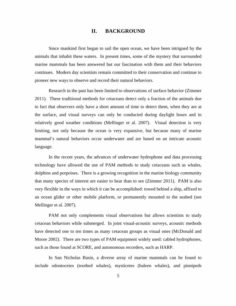
II. BACKGROUND

Since mankind first began to sail the open ocean, we have been intrigued by the

animals that inhabit these waters. In present times, some of the mystery that surrounded

marine mammals has been answered but our fascination with them and their behaviors

continues. Modern day scientists remain committed to their conservation and continue to

pioneer new ways to observe and record their natural behaviors.

Research in the past has been limited to observations of surface behavior (Zimmer

2011). These traditional methods for cetaceans detect only a fraction of the animals due

to fact that observers only have a short amount of time to detect them, when they are at

the surface, and visual surveys can only be conducted during daylight hours and in

relatively good weather conditions (Mellinger et al. 2007). Visual detection is very

limiting, not only because the ocean is very expansive, but because many of marine

mammal’s natural behaviors occur underwater and are based on an intricate acoustic

language.

In the recent years, the advances of underwater hydrophone and data processing

technology have allowed the use of PAM methods to study cetaceans such as whales,

dolphins and porpoises. There is a growing recognition in the marine biology community

that many species of interest are easier to hear than to see (Zimmer 2011). PAM is also

very flexible in the ways in which it can be accomplished: towed behind a ship, affixed to

an ocean glider or other mobile platform, or permanently mounted to the seabed (see

Mellinger et al. 2007).

PAM not only complements visual observations but allows scientists to study

cetacean behaviors while submerged. In joint visual-acoustic surveys, acoustic methods

have detected one to ten times as many cetacean groups as visual ones (McDonald and

Moore 2002). There are two types of PAM equipment widely used: cabled hydrophones,

such as those found at SCORE, and autonomous recorders, such as HARP.

In San Nicholas Basin, a diverse array of marine mammals can be found to

include odontocetes (toothed whales), mysticetes (baleen whales), and pinnipeds

6

(walruses and seals) (Hildebrand et al. 2011). We anticipated detections of odontocetes

that vocalize in the high-frequency range: 8 to 100 kHz. Odontocetes typically found in

San Nicolas Basin include Cuvier’s beaked whales (Ziphius cavirostris), sperm whales

(Physeter macrocephalus), and different delphinid species, including killer whales

(Orcinus orca), Risso’s dolphins (Grampus griseus), and Pacific-white sided dolphins

(Lagenorhynchus obliquidens) (Hildebrand et al. 2011). Below, we discuss the

population, ecology, behavior and vocalization characteristics of some toothed whales,

which are year round or seasonal residents of the Southern California Bight.

A. CUVIER’S BEAKED WHALES (ZIPHIUS CAVIROSTRIS)

Cuvier’s beaked whale is the most common species of beaked whale found in the

Southern California area (Hildebrand et al. 2011). It is estimated that there are

approximately 1,200 Cuvier’s beaked whales along the west coast of the continental

United States (Carretta et al. 2007).

Cuvier’s beaked whales normally inhabit the waters over the continental slope

and deep oceanic water, usually being sighted in waters that are deeper than 200 m

(Jefferson et al. 2008) and are routinely recorded in depths of 1000 m or more (DON

2008).

Cuvier’s beaked whales are long, deep divers and have been recorded conducting

dives that last for almost 1.5 hours and at depths of almost 2 km (Rommel et al. 2006). It

was once thought that Cuvier’s beaked whales only feed at the ocean bottom, but recent

studies have found that they may also feed at mid water levels (DON 2008).

Cuvier’s beaked whales are found in small groups of two to seven, but it is not

uncommon to see them alone or with a group of dolphins (Jefferson et al. 2007). There is

no known calving season. Although not seen every month, beaked whales are found

randomly throughout the year in this area (Dohl 1980).

Cuvier’s beaked whales produce broadband echolocation clicks that are very

distinct from those of any other species and last about 200 µs. Their clicks span over a

frequency range of 20 to 60+ kHz, with the dominant frequency near 40 kHz. Beaked

7

whale clicks have a very distinct upsweep in frequency. This upsweep occurs over a 0.15

ms interval. Their clicks also have a very specific inter-click interval (ICI) of 0.3-0.4 s

(Zimmer 2011).

B. DOLPHIN

The group of delphinids found in the Southern California Bight include short-

beaked common (Delphinus delphis), long-beaked (D. capensis), bottlenose (Tursiops

truncates) dolphins Pacific white-sided (Lagenorhynchus obliquidens), Risso’s (Grampus

griseu) dolphins and others.

Dolphins produce echolocation clicks, buzzes, whistles or combinations of two or

more. Their echolocation clicks are broadband impulses with a frequency range between

20 and 60 kHz (Hildebrand et al. 2011). They typical have no identifiable ICI. Buzzing

is comprised of rapidly repeated clicks. Dolphin whistles are tonal calls that are found

mainly between 5 and 20 kHz.

Only Pacific white-sided dolphins and Risso’s dolphins produce clicks that

contain spectral properties that allow identification down to the species level (Soldevilla

et al. 2008).

1. Risso’s Dolphin (Grampus griseus)

The Risso’s dolphins are widely distributed, inhabiting primarily near shore, deep

waters of the continental slope and outer shelf (DON 2008). There is a minimum

population estimate of 10,000 individuals in the southern California area (Carretta et al.

2007).

Risso’s dolphins have been found to dive down to 600 m (DON 2008) and remain

submerged up to 30 minutes while foraging. They appear to feed mainly at night

(Jefferson et al. 2007).

They are very social animals that are normally found in groups of 30 to several

hundred. Calving seasons differ with populations. The Southern California population

has its calving season in the fall/winter time period.

8

2. Pacific White-Sided Dolphin (Lagenorhynchus obliquidens)

There are two recognized groups of the Pacific white-sided dolphins (PWSD), the

southern and northern groups although these two groups are not visually distinguishable

in the field (DON 2008). It is estimated that a population of over 20,000 of both groups

exist off the western coast of the continental United States (Carretta et al. 2007). These

animals tend to inhabit temperate waters over the outer continental shelf and slope (DON

2008).

PWSD do not appear to be a deep-diving species. Based on feeding habits, it is

estimated that their dives are at least 120 m deep and the majority of foraging dives last

less than 15 to 25 s (DON 2008).

They can be found in groups ranging from tens to thousands, often mixing with

other species such as Risso’s dolphins and northern right whale dolphins (DON 2008).

Calving season occurs during the summer months (Jefferson et al. 2007).

C. SPERM WHALE (PHYSETER MACROCEPHALUS)

The sperm whale is the largest toothed whales species (Jefferson et al. 2007).

There is a minimum population estimate of 1,700 sperm whales along the west coast of

the continental United States (DON 2008). Sperm whales tend to inhabit the continental

slope and waters deeper than 1000 m (Jefferson et al. 2007).

Sperm whales are extremely deep and long divers and have been recorded

reaching depths of 3 km or more and for well over an hour. However, it is more common

for their foraging dives to be about 400 m deep and last 30–45 min (Jefferson et al.

2007).

Most often they are found in medium to large groups of 20-30 whales, with one

bull per breeding group. The females are much more social than the males, traveling in

nursery groups (Whitehead 2003). Most births occur in the summer and fall (Jefferson el

al. 2007). Sperm whales are seasonal migrants through the Southern California Bight

(Dohl 1980).

9

Sperm whales produce clicks, codas and buzzes. Clicks contain energy from 2 to

20 kHz, with the dominant frequency being around 9 kHz. They typically have an ICI of

0.5–2 s (Zimmer 2011). Codas are sequences of clicks but less intense and lower peak

frequencies than regular clicks. Buzzing is comprised of closely spaced clicks

(Hildebrand et al. 2011). Sperm whale clicks are too short to support any frequency

variations. Their clicks are composed of short pulses separated by 3.7 ms. A single pulse

of a sperm whale contains about four oscillations and last about 1 ms (Zimmer 2011).

For this research, we acquired overlapping time periods (June and November

2008) of data from two different recording systems located in close proximity to one

another in the San Nicholas basin. The characteristics of each recording system are

discussed in the data description section.

10


11

III. DATA DESCRIPTION

We used two sets of passive acoustic recordings collected simultaneously and in

close proximity to one another in the San Nicholas Basin via two different recording

systems: a bottom-moored HARP and the NPS recording system at SCORE that receives

data through near-bottom mounted hydrophones. We will refer to these datasets as

“HARP data” and “SCORE data.” The goal was to examine the feasibility of applying

the protocols commonly used for HARP data analysis to SCORE data. We chose to use

the files from data catalogs available to us at the start of this research project that

contained the longest continuously-overlapped periods: June 11–13, 2008 and November

23–27, 2008.

The HARP dataset was gathered by SIO from two separate HARP deployments at

the same location. The other dataset was collected by NPS through one (in June 2008)

and three (in November 2008) hydrophones located within the SCORE network. The

characteristics of each system are discussed below.

A. HARP DATA

HARP is a passive acoustic monitoring system that is capable of recording long-

term, high-bandwidth acoustic data. Currently, these packages are deployed worldwide

in support of long-term behavioral and ecological studies of marine mammals (Wiggins

and Hildebrand 2007).

The HARP device is composed of three main components: a data acquisition

system, a hydrophone sensor and instrument packaging. The data acquisition system is a

low power structure capable of collecting and storing up to 2 TB1 of information per

instrument deployment. It has a sampling frequency of 2 to 200 kHz at 16-bits/sample.

The hydrophone sensor is a broadband (10 Hz–100 kHz) device that can be used to

record acoustic events from low frequency baleen whales vocalizations to high frequency

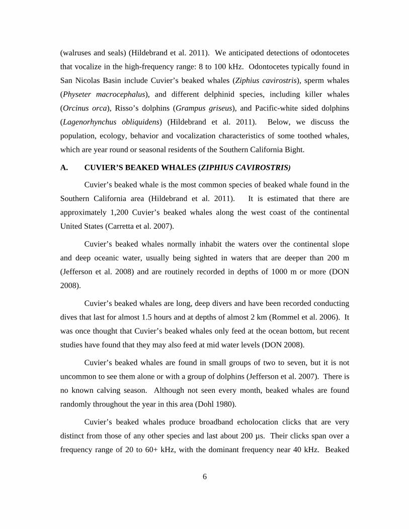
odontocetes echolocation clicks. The instrument packaging (Figure 1) is so designed that

it is compact and easy to deploy and recover (Scripps Whale Acoustic Lab 2007).

1 Hereafter, HARP specifications are given as of 2008 when the data used here were collected.

12

The HARP devices used in this research are owned and operated by SIO in La

Jolla, CA. The data files used were from two separate deployments, both located near the

same site in San Nicolas Basin. The first HARP was deployed from June 4 to August 3,

2008 and located at a depth of 1,012 m. The second one was deployed from October 20

to December 16, 2008 and located at a depth of 1,015 m.

HARP data were continuously recorded for the duration of each deployment at a

sampling frequency of 200 kHz. During the data uploading process, the files were copied

from a specialized file system to a standard system so that the files could be read by a

desktop computer (for more information, see Wiggins and Hildebrand 2007). The files

were then converted into XWAV files with a length of approximately five minutes and

114 MB in size. XWAV files are simply WAV files that have a more robust header that

include information such as latitude and longitude, depth, start and stop times, etc. The

total length of data used in this research from first and second deployments was roughly

52 hours and 81 hours, respectively.

Figure 1. High-frequency Acoustic Recording Package (HARP) seafloor package. The HARP device is composed of three main components: a data acquisition

system, a hydrophone sensor and instrument packaging. (From Wiggins and Hildebrand 2007).

13

B. SCORE DATA

The Southern California Offshore Range complex is located within adjacent

waters to San Clemente Island, CA. San Clemente Island has been owned and operated

by the United States Navy since 1934. SCORE is state-of-the-art, multi-warfare,

integrated training facility that caters to the largest concentration of U.S Navy ships in the

world. The bulk of SCORE operations are designed to support training and readiness

requirements for Third Fleet, it also facilitates the testing, evaluation, and development of

weapon systems and tactics. Within SCORE, lies the instrumented Southern California

Anti-Submarine Warfare Range (SOAR) an anti-submarine warfare (ASW) training

range. The SOAR hydrophone configuration allows for roughly 670 square miles of

underwater tracking area (www.score.com).

SOAR is operated by the Range Operations Center (ROC) personnel at Naval Air

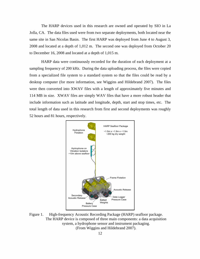
Station North Island, CA (www.score.com). The range hydrophones (Figure 2) are

permanently mounted and acoustic data are streamed back through undersea cables to

San Clemente Island. In cooperation with SCORE Operations, NPS has installed a PAM

recording system that receives data through the SCORE hydrophone network. The NPS

system can digitize a maximum of 32 channels of hydrophones and is controlled remotely

by watch-standers at the ROC. Recording is done on a not-to-interfere with operations

basis.

Due to the hydrophone design, the NPS recording system can simultaneously

record acoustic events between approximately 8 and 40 kHz and at a sampling frequency

of up to 200 kHz. Each channel is patched to a specific hydrophone. One of the

32 channels is always committed to recording a precision timing signal (IRIG-B).

The data used in this research were collected through three range hydrophones

hereafter referred to as SCORE A, SCORE B and SCORE C. All three instruments were

located within a few kilometers of each other and the SIO HARP (Figure 3). SCORE A,

the most northerly, was located at a depth of 1,380 m. SCORE B, which provided data

for both June and November, was located at a depth of 1,498 m. SCORE C, the most

southerly hydrophone, was located at a depth of 1,148 m.

14

In June, the only SCORE data in the vicinity to the HARP that were being

recorded were through hydrophone SCORE B. The data were continuously recorded at a

sampling rate of 96 kHz and written to a hard disk. In November, data from all three

hydrophones were available for our use. SCORE A, B and C data were recorded

continuously at a sampling rate of 80 kHz. The binary format data were converted to

WAV format for visual scanning. The WAV files for June were written in 10 minute

long increments each containing 219 MB of data. November’s files were converted to

WAV files that were 6 minute long and contained 128 MB of data per file. The total

hours available for examination for June and November were approximately 59 and

264 hours, respectively.

Figure 2. SCORE Range Hydrophone diagram (From Science Applications International Corporation MariProOperations 1991).

C. DATA COMPARISON

An important objective of this research was to find, analyze and identify similar

odontocete acoustic events found in both HARP and SCORE datasets that could be used

for identifying the presence of different species through the visual scanning process.

Because the two recording systems had several primary similarities and differences

15

which stem from technical specifications of the instruments and the recording parameters

applied, it was anticipated that the visual cues analysts rely on to identify key

vocalization characteristics of a particular species would be displayed differently in the

HARP and SCORE datasets.

1. Similarities

HARP and NPS recording systems are similar in the fact that they both serve as

passive acoustic monitors. The HARP was specifically built as a passive acoustic

monitoring system. The wide range of species that would likely be encountered was

considered in the design parameters of the system. On the other hand, the primary

function of SCORE is range tracking in support of naval exercises and the passive

acoustic monitoring application is a convenient byproduct. Secondly, both systems

record in the frequency band of interest, though the useful bandwidth for HARP is much

broader than SCORE. For the purpose of passive acoustic monitoring, high frequency is

defined as frequencies at or above 10 kHz. It is in this frequency band that we expect to

find odontocete vocalizations.

HARP and SCORE A, B and C hydrophones were located within close proximity

to one another. Over the period covered in this research, it was anticipated that

vocalizations from the same types of odontocetes would be captured by each system.

HARP is located off range to the west of SOAR. The HARP was 7, 8, and 9 km from

SCORE A, B, and C hydrophones, respectively (Figure 3).

Another similarity between these systems is the fact that we were able to find two

sets of overlapping data: 11 to 13 June 2008 and 23 to 27 November 2008 (Table 1).

Lastly, in this experiment the data were converted into XWAV/WAV files so that

they could be analyzed using a near-identical processing method. XWAV and WAV files

are similar file formats, but the XWAV files have a more robust heading to include

latitude and longitude, depth and start/stop times etc. (Wiggins and Hildebrand 2007).

16

Figure 3. Locations of HARP and SCORE hydrophones A, B and C with bathymetry

Table 1. Dates and total duration of HARP and SCORE data. Total recorded hours of all data available for this research were 456 hours.

JUNE 2008 November 2008 Dates Hours Dates Hours

HARP 13-15 52 23-27 81 SCORE A 23-27 88 SCORE B 13-15 59 23-27 88 SCORE C 23-27 88 Total Hours 111 345

17

2. Differences

The main source of the differences between the HARP and SCORE systems are

what they were designed to do. As noted earlier, HARP was specifically designed for the

passive acoustic recording of marine mammal vocalizations. The capabilities of the

HARP hydrophone are due to the advancements in a low-power, high-data-capacity

computer technology. This package was made to record high frequency mammal

vocalizations on a continuous long-term basis in remote location and independent of the

presence of daylight or weather conditions. The HARP is capable of recording data at a

sampling rate of up to 200 kHz. The 1.92 TB data storage capacity allows the

hydrophone to be deployed for approximately 55 days, when recording continuously at

200 kHz (Wiggins and Hildebrand 2007).

In comparison, the primary purpose of the SCORE hydrophone network is for

range tracking during ASW exercises. The ability to record odontocete vocalizations on

this system is a very beneficial byproduct; however design considerations built in for

operational use are anticipated to affect the system performance as a marine mammal

passive acoustic recording system.

A second difference of these systems is the bandwidth window in which they are

able to record data. HARP records in the 10 Hz to 100 kHz band, whereas SCORE

hydrophones, by design, have more limited bandwidth of approximately 8–40 kHz. This

bandwidth limitation is due to the broadband filter, that suppresses frequencies below

10 kHz and above 40 kHz, that each SCORE hydrophone is outfitted with.

Another important difference between the two systems was the sampling

frequency at which the data were recorded. As mentioned previously, HARP data were

recorded at 200 kHz sampling frequency and SCORE at 96 kHz (June data) and 80 kHz

(November data). This gives Nyquist frequencies at 100 kHz for HARP, 48 kHz (June

data) and 40 kHz (November data) for SCORE.

18

Lastly, SCORE hydrophones are outfitted with an automatic gain control (AGC)

feature. Each hydrophone has an individual AGC adjustment which lowers the

hydrophone response automatically in the presence of strong signals giving them a

broader dynamic range. HARP does not have a similar AGC feature. We do not have

any calibration information on SCORE instruments, unlike HARP which is calibrated

prior to each deployment.

19

IV. METHODOLOGY

An approach applied earlier to other HARP (see Oleson et al. 2007) will be used

to examine HARP and SCORE datasets independently following the below steps.

1. Create long-term spectral averages (LTSAs) for each dataset for 50 Hz

frequency bins and 5 s steps for time averaging.

2. Scan the LTSA to detect marine mammal vocalizations and other sound

sources.

3. Log each detected acoustic event, i.e., document its start and end time,

characteristic frequencies, type of call (whistle, click, buzzing etc.).

4. When possible, classify each acoustic event according to its source, and

identify the vocalizing animal to species.

A. TRITON

Triton is Mathwork’s Matlab based software that was designed to evaluate

acoustics data recorded by Acoustic Recording Packages (ARPs) and HARPs. The data

sets are typically long duration, single channel, continuous or scheduled duty–cycles.

Triton allows users to quickly review these large data sets via a graphical user interface

(GUI). The data sets are transformed into the spectral domain for evaluation as LTSAs

(Triton User Guide 2007).

Triton takes WAV or XWAV files and generates the LTSA files by averaging

spectra over a period of time and arranging these spectra as frequency-time spectrogram

plots. This allows a quick and easy link back to the finer-scale data of the WAV or

XWAV files by clicking on the event of interest in the LTSA plot. It also has a log

feature that allows the users to make a record of an acoustic event and create JPEGs,

WAV and XWAV files (Triton User Guide 2007).

20

B. LONG-TERM SPECTRAL AVERAGES

In order to analyze this data in a practical and timely manner, the Triton program

was used to compress the XWAV and WAV files into LTSAs (Figure 4). LTSAs offer a

way to plot large amounts of data in a compressed format while providing a quick link to

acoustic events in the original XWAV/WAV data. This mitigates the labor intensive and

frankly the unrealistic task of searching through short duration spectrograms for

individual calls.

The LTSA is a three-dimensional time-frequency energy plot where each

frequency spectrum plotted along time is averaged over a longer period than one

windowed frame of a Fast-Fourier Transform (FFT). The averaged spectra are then

plotted sequentially and color coded (Triton User Guide 2007).

In order to create the LTSAs, long-term spectrogram parameters must be set

based on the data sampling rate and target vocalizations. In this research, five seconds

was the length of time chosen to average each time bin and 50 Hz was the frequency bin

size. We chose to make individual LTSAs for each separate day for easy of scanning and

to lessen computation effort it took to create the LTSAs.

Once the LTSAs were created they were displayed in the plot window of Triton

(Figure 4). On the bottom right corner of this window, the LTSA plot details are listed.

Here the sampling rate (Fs), the time average used to create the LTSA (Tave), FFT size

(NFFT), brightness (B) and contrast (C) used to generate the plot are found.

21

Figure 4. Triton’s plot window. Allows users to search for any acoustically significant events. The botton left corner lists the day and time of the file being viewed. The bottom right coner list the plot details of the LTSA.

The control window (Figure 5) contains the controls used to select plot and time

step lengths, to adjust the brightness and contrast, and the buttons used to navigate

through the LTSA and individual XWAV files.

22

Figure 5. Triton control window. Allows users to adjust LTSA plot settings, brightness, contrast, plot length, FFT length, overlap and navigation.

FFT parameters used for different plot length are shown in the corresponding black box.

C. SCANNING

Once an acoustic event of interest was identified in the LTSA, the Triton user

could click anywhere in that event and generated the spectrogram from the original

XWAV/WAV files that correspond to that particular time chosen (Figure 6).

23

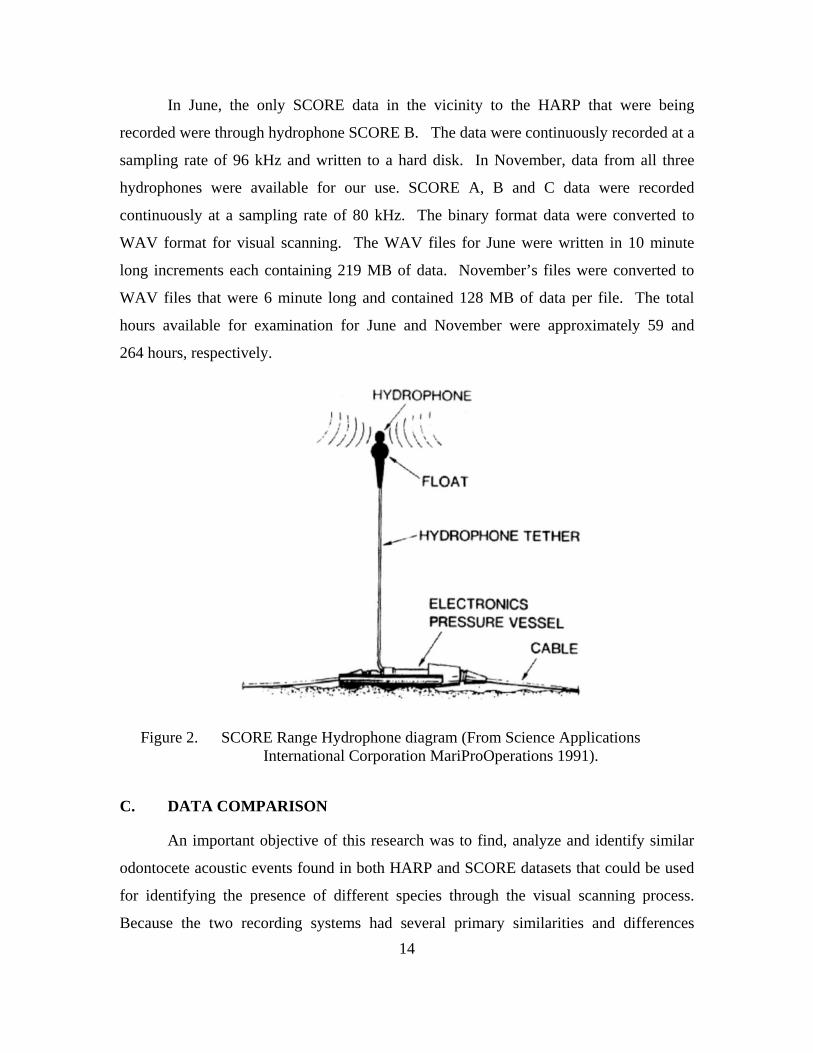
Figure 6. An example of beaked whale detection. An acoustic event of interest was found in the LTSAs (top panel) and once it was clicked on a zoomed in spectrogram (bottom panel) of that event was generated. Notice that the

time scale of the LTSA plot is two hours and the spectrogram is one second length panel.

Once the spectrogram was opened, the control window was updated with the

spectrograms control window. In this research, the FFT settings used were an 85%

overlap, a Hanning window and FFT length of 1000 points. By having the spectrogram

window length at one second, inter-click intervals and peak frequency could be

determined. From here individual clicks were enlarged to determine click length, shape

or if an upsweep was present. This was accomplished by making the window size and

FFT lengths shorter, for example, if window length was 0.1 seconds, we made the FFT

length 256 or if the window length was 0.01 s we made the FFT length 128.

24

Lastly, a time series window and control window were opened by clicking on the

Timeseries radio button at the top of the control window (Figure 5). The time series

window provides a direct plot of the sound pressure measurements. This presentation is a

very useful way to describe signals that express large amplitude variations, such as all

cetacean clicks (Zimmer 2011).

Every HARP and SCORE dataset was scanned independently to ensure marine

mammal detections in each were independently determined without influence form the

other data sets.

D. LOGGING

As we scanned through the data, all acoustic events of interest were logged in an

Excel sheet using Triton’s logger feature. The information on these events of interest

was divided up into categories to include: detections species, call types, start and end

times, frequencies of interest, and comments, and was filed (Figure 7). This function

allowed us to create a record of acoustic events and provided a roadmap to where the

JPEGs and XWAV files were stored. We were also able to sort our log files by species,

call type, start/end times, etc. This allowed us to create simple statistics of the

breakdown of detections by species.

The Excel files were very easy to use with Matlab software. We were able to

create Matlab codes that retrieved the data from the log files and used the data to create

occurrence diagrams, averaged clicks figures and compute statistical analysis on our

information.

25

Figure 7. Excel log file. The log file is a diary of the scanning process. This allows the user to quickly revisit any acoustic event of interest.

E. SPECIES-LEVEL IDENTIFICATION OF ACOUSTIC EVENTS

Identification of detected sounds was based on previously established distinctive

features of specific species vocalizations in HARP data. Beaked whales, dolphins and

sperm whales were the three marine mammals we identified in our scanning. When

scanning SCORE data, we used the HARP based characteristics as a starting point, but

found several differences in feature presentation that are discussed below.

26

1. Cuvier’s Beaked Whale

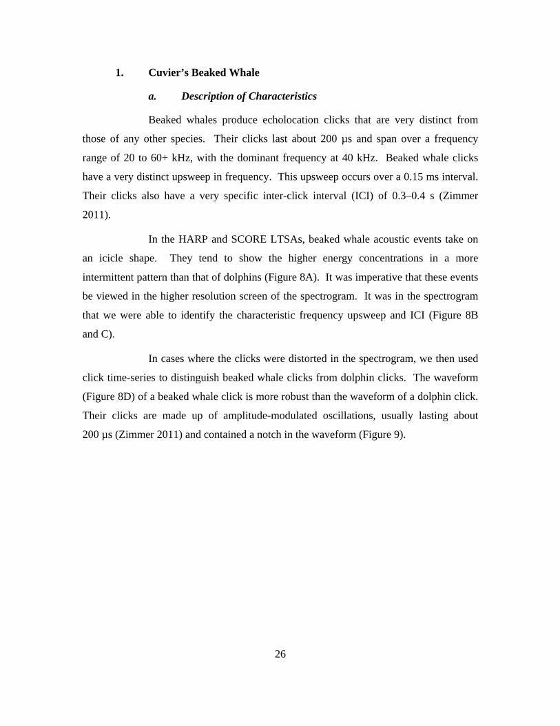
a. Description of Characteristics

Beaked whales produce echolocation clicks that are very distinct from

those of any other species. Their clicks last about 200 µs and span over a frequency

range of 20 to 60+ kHz, with the dominant frequency at 40 kHz. Beaked whale clicks

have a very distinct upsweep in frequency. This upsweep occurs over a 0.15 ms interval.

Their clicks also have a very specific inter-click interval (ICI) of 0.3–0.4 s (Zimmer

2011).

In the HARP and SCORE LTSAs, beaked whale acoustic events take on

an icicle shape. They tend to show the higher energy concentrations in a more

intermittent pattern than that of dolphins (Figure 8A). It was imperative that these events

be viewed in the higher resolution screen of the spectrogram. It was in the spectrogram

that we were able to identify the characteristic frequency upsweep and ICI (Figure 8B

and C).

In cases where the clicks were distorted in the spectrogram, we then used

click time-series to distinguish beaked whale clicks from dolphin clicks. The waveform

(Figure 8D) of a beaked whale click is more robust than the waveform of a dolphin click.

Their clicks are made up of amplitude-modulated oscillations, usually lasting about

200 µs (Zimmer 2011) and contained a notch in the waveform (Figure 9).

27

Figure 8. Beaked whale clicks detected in HARP data: (A) representation of the event in 1-hour long LTSA;

(B) spectrogram of a 1-sec data with two echolocation clicks; (C) spectrogram of a 250 µs long echolocation click;

(D) 1 ms timeseries plot of a single click.

28

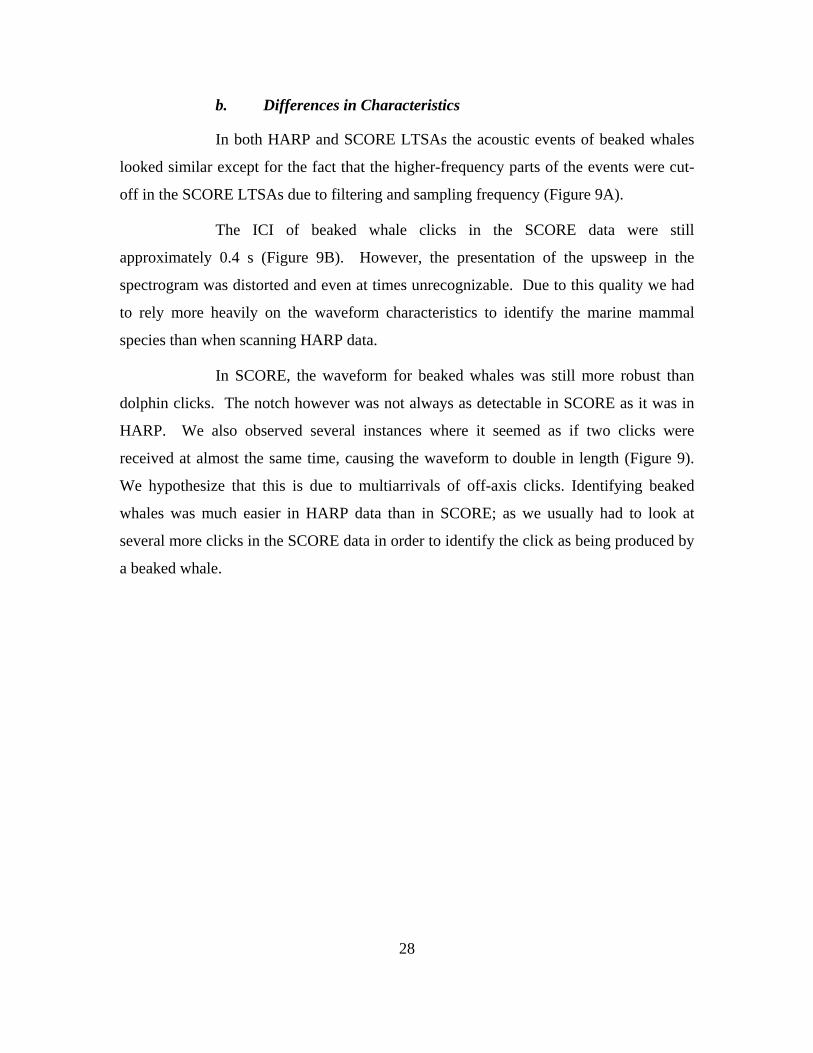
b. Differences in Characteristics

In both HARP and SCORE LTSAs the acoustic events of beaked whales

looked similar except for the fact that the higher-frequency parts of the events were cut-

off in the SCORE LTSAs due to filtering and sampling frequency (Figure 9A).

The ICI of beaked whale clicks in the SCORE data were still

approximately 0.4 s (Figure 9B). However, the presentation of the upsweep in the

spectrogram was distorted and even at times unrecognizable. Due to this quality we had

to rely more heavily on the waveform characteristics to identify the marine mammal

species than when scanning HARP data.

In SCORE, the waveform for beaked whales was still more robust than

dolphin clicks. The notch however was not always as detectable in SCORE as it was in

HARP. We also observed several instances where it seemed as if two clicks were

received at almost the same time, causing the waveform to double in length (Figure 9).

We hypothesize that this is due to multiarrivals of off-axis clicks. Identifying beaked

whales was much easier in HARP data than in SCORE; as we usually had to look at

several more clicks in the SCORE data in order to identify the click as being produced by

a beaked whale.

29

Figure 9. Beaked whale clicks in SCORE B dataset: (A) representation of the event in 1-hour long LTSA; (B) spectrogram of a 1-sec data with three

echolocation clicks; (C) spectrogram of a 200 µs long echolocation click; (D) 2 ms timeseries plot of a single click.

2. Dolphins


Dolphins produce echolocation clicks, buzzes, whistles or a combination

of two or more. Their echolocation clicks are broadband impulses with a frequency

range between 20 and 60 kHz (Hildebrand et al. 2011). They typical have no identifiable

ICI. Buzzing is comprised of rapidly repeated clicks and was sometimes apparent in the

30

LTSA. Dolphin whistles are tonal calls that are found mainly between 5 and 20 kHz.

They vary in frequency modulation and duration (Hildebrand et al. 2011) and were very

visible in the LTSAs (Figures 10 and 11).

Figure 10. Unidentified dolphin vocalizations in HARP: (A) representation of the event in 1-hour long LTSA; (B) spectrogram of a 1-sec data with no clear ICI and buzzing; (C) about a 100 µs spectrogram of individual click; (D) 1-ms timeseries plot of a

single click

31

Figure 11. Unidentified dolphin vocalizations in SCORE: (A) representation of the event in 1-hour long LTSA; (B) spectrogram of a 1-sec data with no clear ICI, buzzing

and whistles; (C) about a 100 µs spectrogram of individual click; (D) 1-ms timeseries plot of a single click

The waveform of the dolphin click is very short, usually only lasting 30 µs

(Zimmer 2011) and made up of less oscillations compared to the beaked whale

waveform. We identified dolphin clicks by not having the characteristics of those of the

beaked whale clicks. The absence of an upsweep in frequency or any identifiable inter-

32

click interval would allow us to categorize the vocalization as belonging to a dolphin. On

several occasions dolphin clicks were accompanied by whistles and/or buzzing, which

provided a good idea that they were dolphins from first glance at the LTSA (Figure 11).

This was then continued by checking the ICI and click duration of the event.

Pacific white-sided dolphins can be identified to species by the distinctive

banding patterns in the LTSA. Their echolocation clicks have energy peaks at 22.2, 26.6,

33.7 and 37.3 kHz (Soldevilla et al. 2008).

Risso’s dolphins can also be identified to species by the distinctive

banding patterns in the LTSAs. Their echolocation clicks have energy peaks at 22.4,

25.5, 30.5, and 38.8 kHz (Soldevilla et al. 2008).


In the LTSAs the acoustic events of dolphins were very similar in both

data sets. How bright the vocalizations appeared in the HARP and SCORE LTSAs were

equal to one another, Figures 10 and 11, respectively. The only difference was the

SCORE device’s auto gain feature sometimes would cut out some of the energy when the

dolphins’ received signal was really strong, which could mean that they were close to the

instrument or that there were numerous animals present. HARP devices do not have this

function.

The lack of a clear ICI in both HARP and SCORE spectrogram was a

clear indicator that dolphins were present. The presence of buzzing and whistles was

always the clearest indicator in both data sets (Figure 11).

In both HARP and SCORE, the waveform of the dolphin echolocation

click appeared shorter and simpler than that of the beaked whale click. We found the

identification process of dolphins in HARP and SCORE to be similar.

33

3. Sperm Whale


Sperm whales produce clicks, codas and buzzes. Clicks contain energy

from 2 to 20 kHz, with the dominant frequency of approximately 9 kHz. They typically

have an ICI of 0.5-2 s (Zimmer 2011). Codas are sequences of clicks but less intense and

of lower peak frequencies than regular clicks. Buzzing is comprised of closely spaced

clicks (Hildebrand et al. 2011). Sperm whale clicks are too short to support any

frequency variations. Their clicks are composed of short pulses separated by about 3.7

ms. A single pulse of a sperm whale contains about four oscillations and last about 1 ms

(Zimmer 2011).

In the LTSAs, we found it quite easy to confuse sperm whales clicks with

anthropogenic (ship) acoustic events. Once the spectrogram was produced, we could

distinguish the continuous, steady sperm whales clicks from the erratic impulses of

mechanical noise and propeller cavitation of a ship. Another way we distinguished sperm

whale clicks from ship noise was to listen to the file. Sperm whale pulses sound like a

metronome, very methodical, whereas ship noise in these frequencies sounds erratic.


In SCORE LTSAs, the acoustic events of sperm whales were distorted due

to the filter roll-off below 10 kHz. This caused the lower-frequency content of the

acoustic events to be cut off, which in several instances made the identification between

sperm whale and anthropogenic (ship) to be very difficult (Figure 12).

The presentations of the sperm whale clicks in HARP and SCORE

spectrograms were comparable. In SCORE data, the lower frequency parts of the clicks

were cut off due to filter roll-off. We also have several instances in SCORE data where

the clicks would span the entire frequency band (up to 40 kHz). In both data sets, the

acoustic event could always be identified as sperm whale by listening to the file. In both

HARP and SCORE sperm whale clicks sound like a metronome.

34

We did not use the waveform as a way of identifying a sperm whale in

either HARP or SCORE. However, the waveforms appear similar. We found more

sperm whales present on SCORE data than HARP. However, the filter roll-off of

SCORE made it more difficult to identify

Figure 12. Sperm whale vocalizations in SCORE: (A) 1-hour long LTSA; (B) spectrogram of 1-s long data; (C) about a 200 µs spectrogram of a single click; (D) 1 ms

waveform of a single click.

35

V. RESULTS

We analyzed six datasets of passive acoustic recordings independently for the

presence of odontocetes. The total data length was approximately 456 hours, about

30% from HARP recordings and the other 70% from SCORE data. The total duration of

detected marine mammal vocalizations in all datasets was about 140 hours with

approximately 20% and 80% of the detections made in HARP and SCORE recordings,

respectively.

Breakdown of the total detection time between individual datasets by identified

species and vocal elements is shown in Table 2.

Table 2. Marine mammal detections in HARP and SCORE datasets. Percentages are given relative to total duration of an individual dataset.

13–15 JUNE 2008 23–27 NOVEMBER 2008

HARP SCORE (B) HARP SCORE (A) SCORE (B) SCORE (C)hrs % hrs % hrs % hrs % hrs % hrs %

Beaked Whale

1.93 3.7 11 18.6 1 1.2 1.8 2.1 4.6 5.3 4.4 5.2

Dolphin 1.2 2.4 3.4 5.6 15.5 18.6 25 29 25.5 29.7 19.1 22.2

Mixed 1.2 2.4 1.5 2.5 9.3 11.4 14.1 16.4 21 24.3 16.7 19.5

Clicks 0 0 1.4 2.3 5.7 7 4.5 5.2 3.9 4.5 1.8 2.1

Whistle 0 0 0.5 .8 0.1 0.1 6.4 7.4 0.7 0.8 0.6 2.1

Sperm Whale

0 0 0 0 4 4.9 3.1 3.5 7 8.2 9.3 10.9

Dataset duration

52 100 59 100 81 100 88 100 88 100 88 100

It is very important for us to define nomenclature as used in this research:

1. Source will refer to a marine mammal species (group of species) or manmade

mechanism, to which a vocalization or sound can be attributed. In this research marine

mammal sources were categorized as beaked whale, dolphin, or sperm whale.

36

Anthropogenic sounds were classified as ship or echosounder. When possible, dolphin

vocalizations were further classified as Pacific white-sided dolphin or Risso’s dolphin.

Those not identifiable to species were logged as “unidentified dolphin.” Sources that we

were unable to classify with high certainty were logged as “unidentified sounds.” In this

research, a conservative approach was applied to species-level identification of detected

sounds. This was done in order to keep the number of false positive identifications low.

We acknowledge that this practice has most likely under-estimated the presence of

certain species.

2. Vocal elements refer to individual distinct sounds or call types to include click,

buzzing (or burst pulse), and whistle that comprise a marine mammal vocalization.

3. Detection/acoustic detection is a presence of a vocalization or anthropogenic

sound in a five second time bin. During the scanning process all attempts were made to

find the very first and last vocal elements of a detected acoustic event (defined below).

Nevertheless, it is likely that event duration was underestimated because vocalizations are

usually weakest (and thus harder to detect) in the beginning and end of an acoustic event.

To account for the possible underestimation, we grouped detections into five second bins

for visualization purposes and statistical estimates.

4. Event/acoustic event is defined as a continuous series of detections that

presumably comes from the same source. In this research, we define continuous to mean

that the maximum separation of neighboring detections do not exceed 30 minutes.

Figures 13–18 show occurrence diagrams categorized by species, time and

recording systems. As can be seen in the diagrams below, there were instances where

events aligned, especially for those of longer duration. This means that conspecific

animals were concurrently detected in different datasets. We are not implying that these

vocalizations are produced by the same individual animal or even the same group of

animals. However, existence of such “concurrent” detections confirms that these species

were present in our area of interest and were successfully detected and identified by us in

different datasets.

37

Below, we analyze species composition of marine mammal detections as well as

the distribution of detections in space (between different instruments) and time (for two

analyzed time periods). This allows us to investigate two questions: which species were

present in our area of interest during the analyzed period and secondly, how coherent the

spatio-temporal variability picture for odontocetes is based on the detections we made in

HARP and SCORE data. The first question is important because the identification

process relies on distinctive features for each species, often with known regional

variations, such as two separate types of Pacific white-sided dolphin echolocations clicks.

The second could be used as a measure of the detection quality. For example,

sperm whales were concurrently detected on 3 of the 4 hydrophones in the November

data set. SCORE C, which located just 4 km from SCORE B, did not have sperm whale

detections. This was an unexpected result because sperm whale echolocation clicks can

be detected at ranges over 10 km. After further analysis of detection results, this

inconsistency was explained. We suspect that sperm whales clicks were registered by

SCORE C hydrophone, but were categorized as unidentified sounds due to the

conservative approach we used to avoid false positive identification.

A. BEAKED WHALES

Although beaked whales tend to travel in smaller groups than dolphins and their

echolocation clicks are very directional, we found numerous vocalizations in both HARP

and SCORE data that were identified as those produced by beaked whales. All beaked

whale detections were categorized as clicks.

Based on known specific features of echolocation clicks, we concluded that most

of the beaked whale vocalizations can be attributed to Cuvier’s beaked whale (Ziphius

cavirostris). As will be discussed below, SCORE recordings of beaked whale clicks

contained enough information to make the same conclusion for the SCORE detections.

1. Seasonal Differences

During the June time period, beaked whale vocalizations made up more than half

of all marine mammal detections, 61% and 77% for HARP and SCORE B data sets,

respectively. The percentages of beaked whale vocalizations for the November time

38

period were much lower in all datasets. Only 5% of all marine mammal detections in the

November HARP dataset were identified as beaked whale clicks. This rate was equal to

6, 12 and 14% for SCORE A, B, and C datasets, respectively.

Since durations of beaked whale detections were comparable for individual June

and November datasets (Table 2), the difference in the presence rate of beaked whales

between these two time periods can be explained by a higher presence rate of dolphins

and sperm whales in November rather than seasonal patterns in beaked whale migration.

This is supported by the fact that Cuvier’s beaked whales are known to be present

throughout the year in the Southern California Bight (Dohl 1980).

2. Spatial Differences

In the June 2008 data, HARP and SCORE B instruments recorded 5 and 23

beaked whale events, respectively. In one instance, beaked whales were detected

concurrently in both datasets. In the November 2008 data, HARP, SCORE A, B, and C

instruments recorded 3, 8, 9 and 10 beaked whale events, respectively. In five instances

beaked whale vocalizations were recorded concurrently in SCORE B and SCORE C

datasets, which are separated by the least distance of all instruments in this research.

Concurrent detections of conspecific animals were made once in all four datasets. The

longest vocalization event lasted 70 minutes and was detected in the SCORE B dataset.

We can attribute the above differences in the detection rate to high directionality of

beaked whale echolocation clicks, distance between hydrophones, and hydrophone depth.

SCORE B hydrophone was located at the deepest depth of approximately 1500 m.

B. DOLPHINS

Dolphins usually travel in large groups and are very social animals, making their

vocalizations very loud. They are also very numerous in the area surrounding the San

Nicholas Basin. Thus as expected, multiple vocalizations in all datasets were identified

as those produced by dolphins. We were able to identify four acoustic events as Pacific

white-sided dolphin (Lagenorhynchus obliquidens). Two of the events were found in

June HARP data, one event in November HARP data and one event in November

SCORE C data. Three of these PWSD vocalizations contained clicks only, the other

39

found in June HARP events contained mixed vocalizations. We did not find any acoustic

events that we were able to identify as Risso’s dolphin.

Vocal elements comprising detected dolphin vocalizations were more diverse than

those of beaked whales. In all datasets, most dolphin detections were identified as mixed.

Mixed vocalizations simultaneously contained clicks and whistles, clicks and buzzing or

a combination of all three. In the June HARP dataset all vocalizations were classified as

mixed. The dolphin vocalizations in June SCORE B data were comprised of 45% mixed,

41% clicks and 14% whistles.

In the November datasets, vocal elements of detected dolphin vocalizations was

distributed as follows: 61% mixed, 38.5% clicks and 0.5% whistles in HARP data;

57% mixed, 18% clicks and 25% whistles in SCORE A data; 82% mixed, 15% clicks and

3% whistles in SCORE B data; 82% mixed, 9% clicks and 9% whistles in SCORE C

data. Vocal activity of dolphins exhibited clear diel variability, with the majority of

vocalizations occurring during the night.

1. Seasonal differences

In the June time period dolphin vocalization detections made up 39% and 23% of

all marine mammal detections for HARP and SCORE B datasets, respectively. These

rates were even higher for November time period: 76, 84, 69 and 58% for HARP,

SCORE A, SCORE B, and SCORE C datasets, respectively.

It is difficult to relate the observed seasonal difference in dolphin detections in

this research to the established patterns of dolphin presence in the Southern California

Bight for three reasons: First, there were only four events that we identified specifically

as Pacific white-sided dolphin, and different delphinid species can exhibit different

seasonal patterns. Secondly, the dolphin distribution in the Southern California Bight

changes from season to season depending on ocean conditions and prey availability, with

a more homogenous distribution during summer/fall (Hildebrand 2009). Lastly, the

analyzed November data covered five days compared to the two days in June, thus

increasing the chances of dolphin presence/detection in this area in November.

40

2. Spatial Differences

In the June 2008 data, we detected three acoustic events in each of the HARP and

SCORE B datasets. Most HARP detections were comprised of mixed vocalizations,

whereas SCORE B detections consisted of either clicks or whistles only. All detected

events were short, not exceeding 42 min. There were no instances in which two

hydrophones recorded conspecifics at the same time.

In the November 2008 data, HARP and SCORE A, B, C recorded 11, 14, 11, and

8 dolphin vocalizations, respectively. In six instances, conspecific animals were detected

on at least two instruments concurrently. SCORE hydrophones detected the longest

dolphin events (500 min by SCORE B and 322 min by SCORE C). Most mixed

vocalizations and all whistles were detected in SCORE data with HARP detections being

comprised of either mixed or clicks only. There was no significant difference in spatial

distribution of detections between datasets from different SCORE hydrophones.

C. SPERM WHALES

We did not find any sperm whale vocalizations for the 13–15 June time period in

either HARP or SCORE B datasets. In November data, most detected sperm whale

vocalizations were categorized as clicks, although a single case of buzzing was detected

in SCORE B.

SCORE C hydrophones did not have any sperm whale detections in November.

However, there were unidentified sound detections in SCORE C at the same time period

when concurrent detections were made on other hydrophones. We hypothesize, due to

our conservative approach in marine mammal identifying; it would be consistent that

these unidentified sounds could be sperm whale vocalizations.

1. Seasonal differences

In the November time period, about 19% of all marine mammal detections in

HARP data were identified as sperm whale vocalizations. These rates were equal to 10,

19, and 28% for SCORE A, SCORE B, and SCORE C datasets, respectively.

41

We attribute the temporal variability to the difference in length between June and

November datasets and to the fact that sperm whales are seasonal migrants through the

Southern California Bight (Dohl 1980).

2. Spatial differences

In the November 2008 data, no sperm whale detections were made in SCORE C

data. HARP, SCORE A and B recorded 2, 3 and 5 sperm whale events, respectively. In

two instances, all three instruments recorded vocalizations of conspecific animals. This

high rate of concurrent detections of conspecific whales can be explained by high source

level of sperm whale sounds, which can be detected at distances of several tens of

kilometers (Barlow and Taylor, 2005; Mellinger at al., 2007).

D. ANTHROPOGENIC

A single detection of ship noise was made in each of the HARP and SCORE B

datasets. These two events were close to one another. Seven ship detections were made

in November. Three of those detections were concurrent.

There was one echosounder detection in June and six in November. All

echosounder detections were concurrent.

E. UNIDENTIFIED SOUNDS

In June 2008 unidentified sounds were detected only in SCORE B data. There

were ten unidentified sound events found in SCORE B data.

In November 2008 dataset, approximately 2% and 4% of total detections

remained unidentified in HARP and SCORE data, respectively. There were four

instances where unidentified sounds were detected in HARP in SCORE datasets

concurrently.

42

Figure 13. Occurrence diagram of beaked whale detections in June and November 2008 data. Green is for HARP detections and blue for

SCORE A, B and C hydrophone detections.

Figure 14. Occurrence diagram of dolphin detections in June and November 2008 data. Green is for HARP detections and blue for S

CORE A, B and C hydrophone detections.

43

Figure 15. Occurrence diagram of sperm whale detections in June and November 2008 data. Green is for HARP detections and blue for


Figure 16. Occurrence diagram of ship detections in June and November 2008 data. Green is for HARP detections and blue for


44

Figure 17. Occurrence diagram of echosounder detections in June and November 2008 data. Green is for HARP detections and blue for


Figure 18. Occurrence diagram of unidentified sound detections in June and November 2008 data. Green is for HARP detections and blue for


45

VI. DISCUSSION

We visually scanned 456 hours of data from two HARP deployments and three

SCORE hydrophones collected from two different seasons over a period of eight days.

As we summarize this research, we can categorize all of the information processed into

three groups: what we anticipated, what we did not anticipate and what we learned.

A. WHAT WE ANTICIPATED

We detected and identified those odontocetes that vocalize in the frequency bands

of interest and are known to be either transient or resident in the Southern California

Bight area. We detected beaked whales, dolphins, and sperm whales. Four of the

detected dolphin events were identified to species as Pacific white-sided dolphins. We

did not find any unexpected marine mammals.

Dolphins are very talkative and boisterous animals that tend to travel in large

numbers, sometimes in the thousands. Beaked whales tend to travel in small groups,

from two to seven members, and produce echolocation clicks that are very directional.

Due to these characteristics, we expected that we would find more dolphin than beaked

whale detections. In this research, we found almost four times the amount of hours of

dolphin detections as beaked whale detections.

Dolphins tend to feed at night and thus we expected to find the majority of

dolphin echolocation clicks and buzzing to occur during this time. Dolphin detections

found in this research exhibited a very pronounce diel variability.

The longer the event duration the more likely it would be recorded on more than

one instrument concurrently. Comparing HARP and SCORE event occurrence between

November (5 days) and June (2 days) (see Figure 14 for an example), we can see that the

November data contained longer events and almost three times the amount of detections,

which were attributed to conspecific animals.

We expected that the SCORE hydrophones that were closer in distance would

have more concurrent detections of conspecific animals than those further apart. In this

data, we saw that such detections from SCORE A/B and SCORE B/C, which were 10 and

46

4 km apart, respectively. There was only one event captured concurrently by SCORE

A/C, which are 13 km apart. There were however, six events captured by all three

SCORE hydrophones.

B. WHAT WE DID NOT EXPECT

SCORE hydrophones had a higher percentage of detections over the recording

period than HARP (Table 2): in June, beaked whale detection rate was 18.6% and 3.7%

in SCORE and HARP data, respectively; in November, these numbers were 4.2% vs.

1.2%. Possible reasons SCORE hydrophones captured more beaked whale detections

than expected was due to the AGC feature these hydrophones are outfitted with, as well

as location and the deeper depth of SCORE hydrophones. Further investigation is

warranted.

November datasets had much more activity than June. As we went through the

datasets, scanning and identification skills improved. We wanted to ensure that the reason

June lacked detections was not due to human error, so we scanned June datasets twice:

once in the beginning and for a second time after we had completed November’s datasets.

However, our second scanning of June data also indicated a sparse amount of marine

mammal vocalizations present.

We also had three times the hours of November data than we had of June for this

research. Although we understand that the shorter the data duration, the less

representative of marine mammal behaviors it is, we were still surprised by the difference

in the number of detections. We hypothesize that these differences are combined effect

of seasonality in odontocete presence, patchiness of their distribution due to difference in

environmental conditions (including prey availability) as well as limited duration of

analyzed data sets.

We did not find any sperm whale detections in June but found 23 hours of sperm

whale vocalizations in November. We attribute the temporal variability in the sperm

whale detections to known randomness of year-around sperm whale presence in the

Southern California Bight (Dohl 1980), and difference in length of June and November

datasets.

47

We did not find any Risso’s dolphin vocalizations in any of our datasets. Risso’s

dolphins are one of the two dolphin species that can be identified to species by the

spectral content of their clicks. We surmise the reason we did not detect them was not

because of the recording system’s limitations but because they just were not physically

present in close proximity to our instruments during the analyzed time periods.

SCORE had a higher percentage of unidentified sound detections per total

detections in each dataset, 11 and 4% in June and November, respectively. We suspect

that most of these unidentified sounds are marine mammal vocalizations and even think

that they may have been distorted beaked whale clicks. However, because we chose a

conservative approach to limit false positives in this research, we chose to “err on the side

of caution” and leave these detections as unidentified.

C. WHAT WE LEARNED

Although we expected there would be performance differences between SCORE

and HARP instruments, we also learned that each of the three SCORE hydrophones

responded differently. SCORE A and B had sensitivity bands at different frequencies,

whereas SCORE C had a flatter response than SCORE A or B. These differences

produce slightly different characteristics of the displayed signal.

We were also able to list the features of beaked whale and Pacific white-sided

dolphin echolocation clicks as presented in SCORE data. Received beaked whale clicks

were affected in two major ways. There was a flattening of the characteristic upsweep

due both to hydrophone filtering and using a Nyquist frequency near the peak frequency.

The second way is that the click spectra were also altered by narrowing the spectral peak

bandwidth and shifting the peak frequency. However, ICI and click duration maintained

the same characteristics as published results.

The Pacific white-sided dolphin presented the signature alternating high and low

amplitude bands in the spectrograms at the frequencies associated with PWSD.

However, the first spectral peak of the two PWSD acoustic events recorded by SCORE A

and B detections were elevated by receiver sensitivity bands that are present in these

hydrophones. This is discussed in more details below.

48

1. Individual Instrument Characteristics and their Effects

This section summarizes each instrument’s dataset by plotting the whole record

on a single LTSA, and discusses the apparent peculiarities of instruments and how results

of marine mammal detection/identification were affected by these characteristics.

Figures 19-24 show LTSAs for individual datasets. In order to provide a figure in which

acoustic events were easily distinguished we adjusted contrast and brightness of each

figure as it is typically done in Triton. Figure 25 shows mean spectral content of each

datasets, which was calculated by averaging corresponding LTSAs over the total length

of each dataset.

a. HARP

The HARP LTSA for June is shown in Figure 19. There was unidentified

noise present throughout the dataset in 24 to 31 kHz frequency band with several

pronounced harmonics at approximately 27 and 28 kHz. The noise is represented by the

bright yellow bands on the LTSA. This noise made it difficult to visually detect acoustic

events at these frequencies because the intensities of the noise masked the most important

feature of marine mammal vocalizations. The power spectra curve (Figure 25) for June

shows a combined effect of the noise and marine mammal vocalization in 25-35 kHz

frequency band.

HARP LTSA for November is show in Figure 20. The LTSA shows the

data lacked both distracting background noise and marine mammal vocalizations. The

corresponding power spectra curve (Figure 25) is relatively flat and does not display

pronounced maximums or minimums.

49

Figure 19. HARP LTSA for June 2008. The LTSA parameters are shown by the legend located in the right lower corner of the spectrogram.

50

Figure 20. HARP LTSA for November 2008. The LTSA parameters are shown by the legend located in the right lower corner of the spectrogram.

51

b. SCORE A

SCORE A LTSA for November, 2008 has a band of elevated intensity that

spans from approximately 22 kHz to 29 kHz. We hypothesized that this band is a

combined result of two effects: enhanced sensitivity of the hydrophone and odontocete

clicks present in this frequency band. In turn, this may affect results of data scanning.

This sensitivity band, seen as a light blue band around 25 kHz, could make it easier to

visually detect marine mammal vocalizations in the LTSAs. However, it could make

identification of marine mammal vocalizations more difficult by shifting how peak

intensity values are displayed. The effects of this sensitivity band are discussed in more

detail when we discuss beaked whale and PWSD click features below.

The power spectra curve (Figure 25) for SCORE A has three peaks. The

first peak occurs at 10 kHz. We speculate that this peak happens because of the acoustic

events that occur in the bins between 10 and 15 kHz. The second peak occurs at

approximately 23 kHz. We hypothesize the reason for this peak is the instrument’s

sensitivity band amplifying the marine mammal vocalizations present. The third peak

occurs at 38 kHz. We suspect this peak is formed due to the filter that suppresses

frequencies above 40 kHz.

52

Figure 21. SCORE A LTSA for November 2008. The LTSA parameters are shown by the legend located in the right lower corner of the spectrogram.

c. SCORE B

SCORE B instrument appears to have a sensitivity band that spans from

approximately 22 kHz to 24 kHz (Figures 22 and 23). As with SCORE A, this sensitivity

band, seen as a light blue band between 20 and 25 kHz, could make it easier to detect

53

marine mammal vocalizations near this frequency (in LTSAs). However, it could make

identification of marine mammal vocalizations more difficult by shifting the displayed

peak frequency value. This sensitivity band appears in the same place in both June and

November LTSAs.

The power spectra curve (Figure 25) for November SCORE B datasets

also has three peaks. The first peak occurs at 10 kHz. We suspect this peak occurs due

to high intensity acoustic events that occurred on the 24 and 26 of November (seen as the

dark red forms on Figure 23) and because of the broadband filter that suppresses

frequencies below 10 kHz. The second peak occurs at approximately 22 kHz. We

suspect the reason for this peak is the instrument’s sensitivity band amplifying the marine

mammal vocalizations present. The third peak occurs at 38 kHz. We suspect this peak

occurs due to the broadband filter that suppresses frequencies above 40 kHz.

June SCORE B power spectra curve has relatively the same shape, but the

overall intensity values are much lower due to less events overall and the sampling

frequency. The three peaks occur at the same frequencies as November SCORE B’s. We

speculate that the first and third peaks of the spectra are caused by the broadband filter

for frequencies below 10 kHz and above 40 kHz. The second peak also occurs at

approximately 22 kHz. We suspect the reason for this peak is the instrument’s sensitivity

band amplifying the marine mammal vocalizations present.

54

Figure 22. SCORE B LTSA for June 2008. The LTSA parameters are shown by the legend located in the right lower corner of the spectrogram.

55

Figure 23. SCORE B LTSA for November 2008. The LTSA parameters are shown by the legend located in the right lower corner of the spectrogram.

56

d. SCORE C

SCORE C was the only hydrophone that did not have a sensitivity band

(Figure 24). No vocalizations were intensified due to sensitivity issues as discussed

above in SCORE A and B.

The power spectra curve for SCORE C had only two peaks (Figure 25),

which are less pronounced than those for two other hydrophones. The first peak occurs at

approximately 8 kHz. We speculate that reason for this first peak is the acoustic event

that occurred on 26 November (Figure 24). The second peak occurs at 38 kHz. We

suspect this peak occurs due to the filter that suppresses frequencies above 40 kHz.

57

Figure 24. SCORE C LTSA for 23-27 November 2008. The LTSA parameters are shown by the legend located on the right side of the spectrogram.

58

Figure 25. Mean spectral content by instrument and season. The power spectra curves were calculated by averaging corresponding LTSAs over individual datasets.

2. Characteristics of Marine Mammals’ Vocalizations Recorded by SCORE Instruments

In order to species-level identify marine mammal vocalization acoustically, it is

important to establish invariant and distinctive features of their vocal elements.

Vocalization features already established for certain marine mammals on one recording

system may appear modified due to specific operating characteristics of another system.

This section describes beaked whale and Pacific white-sided dolphin click characteristics

as presented in SCORE data.

Cuvier’s beaked whales and PWSD dolphins are the two odontocetes found in our

datasets that have published click features. Beaked whale clicks are identified by an

inter-click interval of ~0.4 s, an upsweep in frequency from 20 to 60 kHz with the peak

frequency at 40 kHz, click duration of at least 200 µs and a deep notch at approximately

59

26 kHz in the spectra (Zimmer 2011). PWSDs are identifiable to species by the presence

of four characteristic spectral peaks at 22.2, 26.6, 33.7 and 37.3 kHz and three

characteristic spectral notches at 19, 24.5 and 29.7 kHz (Soldevilla et al. 2008) in their

clicks.

The examples discussed in this section are not meant to be representative of the

species as a whole or even a specific population. Due to the limited amount of data used

in this research, click samples taken from an individual dataset for a certain species, are

most likely produced by several animals (or a group of animals) at most. Thus the

examples in this section certainly may contain characteristics of individual animals.

However, this approach allows us to answer two important questions. How are

distinctive features presented in SCORE data and do the features still allow us to identify

specific species? How are these vocalization features distorted by the SCORE recoding

system?

a. Beaked Whale

1. Interclick interval To estimate the interclick interval from

SCORE dataset, we drew approximately 100 clicks from each dataset and calculated a

sample median and its interquartile range. As seen from the box plot for different dataset

(Figure 26), ICI values for both HARP and SCORE data fit primary within the 0.3-0.6 s

range, which is a known robust feature of Cuvier’s beaked whale (Zimmer et al. 2005).

HARP June data had higher variance in ICI length whereas HARP

November had the least variance. SCORE A’s sample median was the closest to the

0.4 s. SCORE B June had most outliers, which were ICI lengths calculated to be 1.5

times the interquartile range away from the top or bottom of the box. SCORE B

November and SCORE C November had closest ICI interquartile values of all the data

sets.

Note that most outliers lie above the top of the box but none are

lower than 0.25 s. It is known that beaked whale sometimes cease their click sequences

for longer than 1 s, and thus higher ICI values are possible when averaged over the click

60

train (Zimmer et al. 2005), while ICI less than 0.2 s would raise suspicion that the

vocalization was not produced by a beaked whale.

Caution should be taken however when interpreting the above

statistics as they can be highly biased by representing individual characteristics of several

individual whales in each dataset but not the species/population as a whole. Nevertheless,

we can conclude that the mean interclick interval value of 0.43±0.092s (Zimmer et al.

2005) is still a highly robust feature of Cuvier’s beaked whale clicks as recorded by

SCORE instruments, and can be used to distinguish these animals from other odontocete

species.

2. Duration and spectral content of an echolocation click

Beaked whale clicks are very directional, so clicks that are not

received by the hydrophone on-axis can become distorted and suffer transmission loss

(Zimmer et al. 2005). The criteria for choosing a click was it had to be somewhat in the

middle of the click train and have a strong signal. We selected one click from both

SCORE B and SCORE C data to see how sampling frequency and an existence of

sensitivity bands would affect clicks. SCORE B data were recorded at a sampling

frequency of 96 kHz and has a sensitively band along the 22 to 24 kHz frequency range.

SCORE C data was recorded at a sampling frequency of 80 kHz and lacked a sensitivity

band. Note both hydrophones are equipped with a filter that suppresses signal above

40 kHz.

Spectrograms, time series and power spectral density estimates of a

beaked whale clicks found in SCORE B and SCORE C datasets were plotted to analyze

how click length, upsweep and spectral content of beaked whale clicks were affected by

the individual hydrophone characteristics (Figures 27 and 28).

Spectrograms of individual clicks were calculated from recording

clips of 0.1 s length using a Hanning window and FFT with 32 samples and 31 samples

of overlap, and plotted in upper panels of Figures 27 and 28 for June SCORE B and

November SCORE C datasets, respectively. Two features were examined using these

spectrograms: the shape and bandwidth of the clicks upsweep feature and the value of the

peak frequency.

61

The SCORE B spectrogram has a distinctive upsweep in frequency

that is typical of a beaked whale echolocation click, which goes from 20 to 60+ kHz over

a 0.15 µs interval (Zimmer 2011). We hypothesize that the upsweep feature has been

slightly flattened by the SCORE hydrophone filter that suppresses signals above of

40 kHz reducing the signal received from the higher-frequency part of the beaked whale

click (i.e., from 40 to about 60 kHz).

The beaked whale click from SCORE C (Figure 28) also presents

the upsweep feature but has been flattened even more so than the click from SCORE B

(Figure 27). We hypothesize the reason behind the flattening of the spectrogram form is

twofold. First the broadband filter applied to all SCORE hydrophones for frequencies

above 40 kHz changed the shape as in SCORE B data. Secondly, SCORE C was set to

record acoustic events at a sampling rate of 80 kHz in November. Since the Nyquist

frequency was about the same as the filter some of the high-frequency portion of the

beaked whale click was folded due to aliasing.

Beaked whale clicks are known to have duration of around 200 µs,

whereas most dolphin clicks last between 20 and 100 µs (Zimmer et al. 2005). The time

series of beaked whale clicks are shown in the bottom left panel of Figures 27 and 28 for

June SCORE B and November SCORE C datasets, respectively.

The duration of beaked whale click found in SCORE was

approximately 240 µs. In SCORE C the beaked whale click had duration of

approximately 300 µs. In both cases the click duration parameter for beaked whale

identification holds true, and can be used as a distinctive feature for identification of

beaked whale echolocation clicks.

In order to be classified as a beaked whale echolocation click, a

click should have a spectral bandwidth from 20 to 60 kHz with a peak at 40 kHz (Zimmer

et al. 2005) and a pronounced (about 20 dB) spectral notch at about 26 kHz. Estimated

Welch power spectral densities are shown in lower right panels of Figures 27 and 28 for

June SCORE B and November SCORE C data, respectively.

The beaked whale click from SCORE B has spectral bandwidth

from about 31 to 38 kHz and a spectral peak around 35 kHz (Figure 27). The spectral

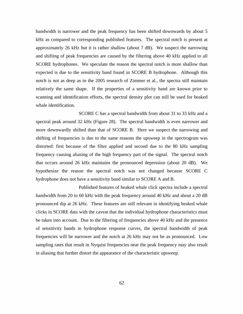
62

bandwidth is narrower and the peak frequency has been shifted downwards by about 5

kHz as compared to corresponding published features. The spectral notch is present at

approximately 26 kHz but it is rather shallow (about 7 dB). We suspect the narrowing

and shifting of peak frequencies are caused by the filtering above 40 kHz applied to all

SCORE hydrophones. We speculate the reason the spectral notch is more shallow than

expected is due to the sensitivity band found in SCORE B hydrophone. Although this

notch is not as deep as in the 2005 research of Zimmer et al., the spectra still maintain

relatively the same shape. If the properties of a sensitivity band are known prior to

scanning and identification efforts, the spectral density plot can still be used for beaked

whale identification.

SCORE C has a spectral bandwidth from about 31 to 33 kHz and a

spectral peak around 32 kHz (Figure 28). The spectral bandwidth is even narrower and

more downwardly shifted than that of SCORE B. Here we suspect the narrowing and

shifting of frequencies is due to the same reasons the upsweep in the spectrogram was

distorted: first because of the filter applied and second due to the 80 kHz sampling

frequency causing aliasing of the high frequency part of the signal. The spectral notch

that occurs around 26 kHz maintains the pronounced depression (about 20 dB). We

hypothesize the reason the spectral notch was not changed because SCORE C

hydrophone does not have a sensitivity band similar to SCORE A and B.

Published features of beaked whale click spectra include a spectral

bandwidth from 20 to 60 kHz with the peak frequency around 40 kHz and about a 20 dB

pronounced dip at 26 kHz. These features are still relevant in identifying beaked whale

clicks in SCORE data with the caveat that the individual hydrophone characteristics must

be taken into account. Due to the filtering of frequencies above 40 kHz and the presence

of sensitivity bands in hydrophone response curves, the spectral bandwidth of peak

frequencies will be narrower and the notch at 26 kHz may not be as pronounced. Low

sampling rates that result in Nyquist frequencies near the peak frequency may also result

in aliasing that further distort the appearance of the characteristic upsweep.

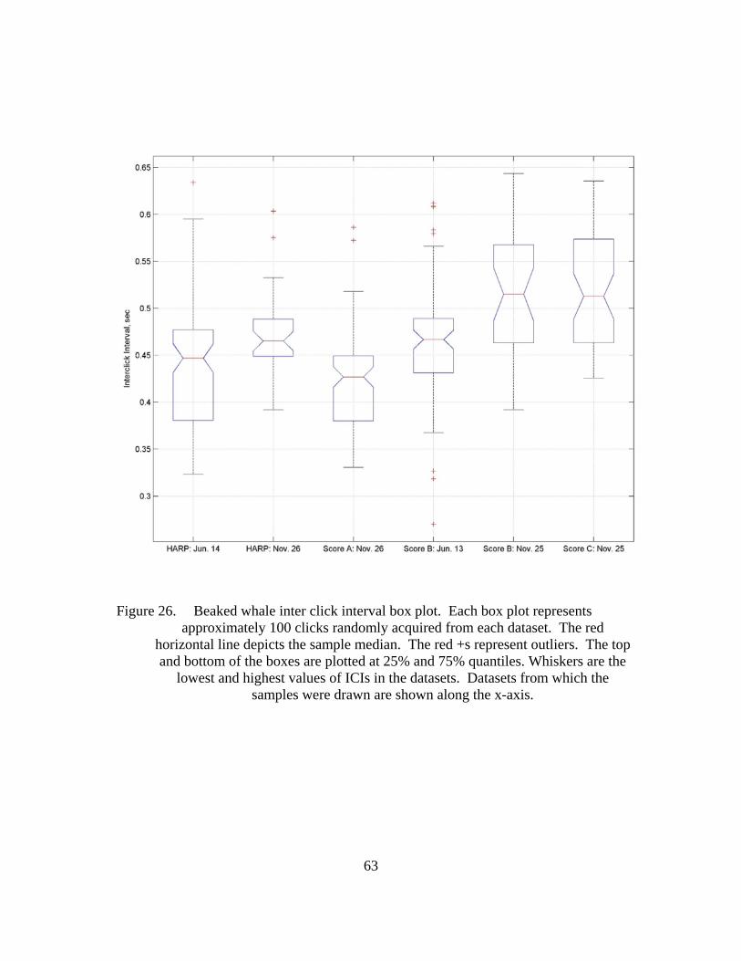
63

Figure 26. Beaked whale inter click interval box plot. Each box plot represents approximately 100 clicks randomly acquired from each dataset. The red

horizontal line depicts the sample median. The red +s represent outliers. The top and bottom of the boxes are plotted at 25% and 75% quantiles. Whiskers are the

lowest and highest values of ICIs in the datasets. Datasets from which the samples were drawn are shown along the x-axis.

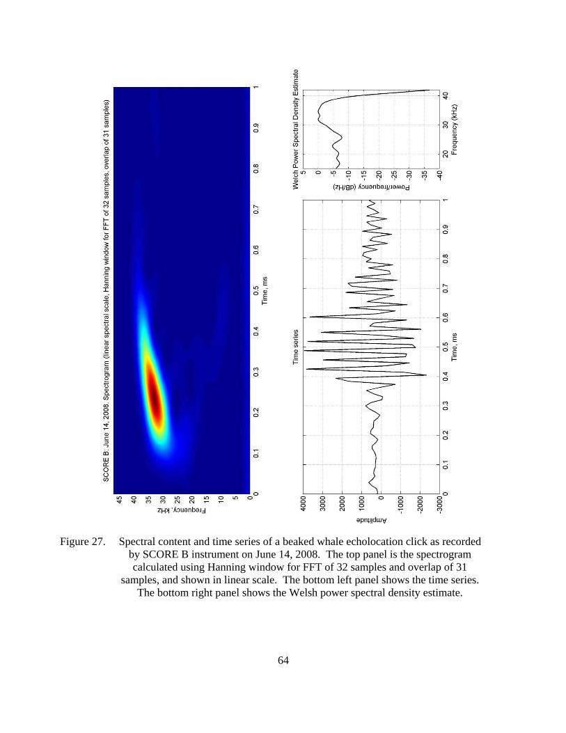
64

Figure 27. Spectral content and time series of a beaked whale echolocation click as recorded by SCORE B instrument on June 14, 2008. The top panel is the spectrogram calculated using Hanning window for FFT of 32 samples and overlap of 31

samples, and shown in linear scale. The bottom left panel shows the time series. The bottom right panel shows the Welsh power spectral density estimate.

65

Figure 28. Spectral content and time series of a beaked whale echolocation click as recorded by SCORE B instrument on November 25, 2008. The top panel is the

spectrogram calculated using Hanning window for FFT of 32 samples and overlap of 31 samples, and shown in linear scale. The bottom left panel shows the time

series. The bottom right panel shows the Welsh power spectral density estimate.

66

b. Pacific White-Sided Dolphin

Pacific white-sided and Risso’s dolphins are the only two delphinid

species which are presently known to produce echolocation clicks with robust spectral

peaks and notches that can be used for their identification on species-level. Values of the

peak and notch frequencies have been established for free-ranging Pacific white-sided

dolphins typical for Southern California region (Soldevilla et al. 2008). We found a total

of four PWSD events in our datasets. Two events were recorded on SCORE B on 14 and

15 June, one event on HARP on 25 November and one event on SCORE C on

27 November (Figure 29). Each PWSD event had a different duration, with the event

recorded by SCORE C lasting the longest.

The click patterns in these spectrograms show the alternating high and low

amplitude bands that are evident at the frequencies associated with PWSD (Soldevilla et

al. 2008). We compared only the first three peaks and the first two notch values because

the filtering of the SCORE data above 40 kHz suppressed the other peaks and notches.

The patterns are consistent for all four events, although intensity levels differ, on each of

the different instruments.

Figure 30 shows the mean spectral plots averaged over the duration of

each event and normalized for comparison purposes. From these data, mean values of

peak and notch frequencies within 10–40 kHz frequency band were estimated for each

event. Corresponding mean spectral curves (see Figure 25) were also normalized and

superimposed onto each plot in Figure 30 to analyze how different hydrophone responses

affected the peaks and notches of PWSD echolocation clicks.

The 14 June PWSD event on SCORE B had peak frequency values at

21.4, 27.4 and 32.2 kHz and notch frequency values of 19.3 and 26.3 (Table 3). We

surmise that SCORE B’s enhanced sensitivity in the frequencies between 22 and 24 kHz

elevated the first spectral peak of the PWSD vocalization (Figure 30).

The 15 June event on SCORE B had peak frequency values of 21.5,

27.4 and 26.3 kHz and notch frequency values of 16.7 and 26.3 kHz (Table 3). As in the

67

case of the 14 June PWSD event, we attribute the elevation of the first spectral peak to

the enhanced sensitivity of the SCORE B hydrophone.

The PWSD event recorded by HARP on 25 November had peak frequency

values at 21.5, 27.5 and 31.5 kHz and a second notch frequency value of 25.4 kHz (Table

3). The fact that the first two peaks frequency values are close in amplitude follows the

results of Soldevilla et al. (2008). This is due to the flat response of the HARP in the

frequency band (Figure 30).

SCORE C’s 27 November event had peak frequency values at 21.4, 27.5

and 32.1 kHz and a notch frequency value of 25.6 kHz (Table 3). These results also

follow the results from Soldevilla et al. (2008) research and are due to the flat response of

the SCORE C in the frequency band.

Table 3 summarizes the above peak and notch frequencies resolved in the

10 to 40 kHz frequency band in comparison with published results. The values for peaks

two and three of PWSD events found in our data are consistant with the results of the the

second and third peaks in Soldevilla et al. (2008) research, and imply that detected

vocalizations were of Type B.

68

Figure 29. LTSAs of the four PWSD vocalization events in different datasets: (a) SCORE B on June 4, 2008 starting at 10:33am; (b) SCORE B on June 15,

2008 starting at 04:54 am; (c) HARP on November 25, 2008 starting at 12:19 pm; (d) SCORE C on November 27, 2008 starting at 03:02 am. The magnitude of the

spectral content is represented by color. Red color represents the greatest concentration of energy whereas dark blue represents no or very little energy.

Two consistent spectral peaks are evident in each LTSA.

(a) (b) (c) (d)

69

Figure 30. Normalized spectral content of PWSD echolocation clicks averaged over event duration for (a) SCORE B on June 4, 2008; (b) SCORE B on June 15, 2008; (c) HARP on November 25, 2008; (d) SCORE C on November 27, 2008. The gray shaded area is the standard deviation for each plot. Normalized mean spectral curve (averaged over each dataset duration) from Figure 25 has been

superimposed onto each PWSD event’s plot and is represented with a dotted line.

(a)

(b)

(c)

(d)

70

Table 3. Means of local peak and notch frequencies in kHz of PWSD echolocation clicks. Row one contains Soldevilla et al. 2008 means and standard

deviations (in parenthesis) of peaks and notches for PWSD echolocation clicks Types A and B. Rows two through five contain the means for the four PWSD events we found in our datasets. These means were acquired

from corresponding LTSAs over time.

Peak 1 Peak 2 Peak 3 Notch 1 Notch 2 Soldevilla 2008:

Type B Type A

22.2 (0.6)

22.2

26.6 (0.9)

27.4

33.7 (1.4)

33.7

19.0 (1.1)

19.0

24.5 (0.9)

24.5

SCORE B June 14 21.4 27.4 32.2 19.3 26.3 SCORE B June 15 21.5 27.4 33.2 16.7 26.3 HARP Nov 15 21.5 27.5 31.5 25.4

SCORE C Nov 27 21.4 27.5 32.1 14.7 25.6

D. CONCLUSION

This research effort describes how a PAM system not designed to track marine

mammals, such as SCORE hydrophones, performed as compared to a system designed

detect marine mammal vocalizations.

Based on the results discussed in the above sections, we conclude that SCORE

system can be used for passive acoustic monitoring of some odontocetes. In order to

mitigate the effects that individual SCORE hydrophone characteristics may have on

acoustic events, it is imperative that SCORE scanning protocols must be adjusted for

hydrophone performance. Protocols must account for the way the broadband filter and

lower sampling frequencies affect the upsweep and peak frequency of beaked whale

clicks. Sensitivity bands for individual hydrophones must be identified and described in

order to anticipate how spectra will be affected.

The next suggested step in this process is to automate the scanning and detection

process. This will allow for large amounts of data to be more quickly analyzed. As it is

now, scanning these large amounts of PAM data required intensive man hours.

A suggested way forward for automating this process is to construct a set of

specific and invariant rules that replicate the human processing method. These rules

71

would allow a pattern recognition approach to be used to identify and extract species

specific vocalization information from these very large datasets in a timely and efficient

manner.

This information is valuable to the U.S. Navy for determining temporal and

spatial distribution of marine mammals in and near naval training ranges. Understanding

population distribution and its variability can improve understanding of marine mammals

response to sounds generated from naval operations and exercises. This information can

also lead to improved migration procedures that minimize the negative effects on marine

mammals while maintaining fleet readiness.

72


73

LIST OF REFERENCES

Barlow, J., and B. L. Taylor, 2005: Estimates of sperm whale abundance in the northeastern temperate Pacific from a combined acoustic and visual survey. Mar. Mamm. Sci. 21(3), 429–445.

Carretta, J.V., Forney, K.A. Forney, M.S. Lowry, J. Barlow, J. Baker, B. Hanson, and M.M. Muto, 2007: Final U.S. Pacific marine mammal stock assessments: 2007. NOAA Technical Memorandum NMFSSWFSC-414, 316pp.

DON (Department of the Navy), 2008: Marine Resource Assessment for the Southern California and Point Mugu Operation Areas. Pacific Division, Naval Facilities Engineering Command, Pearl Harbor, Hawaii. Contract # N62470-02-D-9997, CTO 120. Prepared by Geo-Marine, INC., Plano, Texas.

Dohl, T.P., K.K. Norris, R.C. Guess, J.D Bryant, and M.W. Hoing, 1980: Summary of marine mammals and seabird surveys of the Southern California Bight area, 1975-1978. Part II. Cetacea of the Southern California Bight. Final Report to the Bureau of Land Management, NTIS Rep. No. PB81248189, 414pp.

Hildebrand, J.A., 2005: Final Report SERDP Project 1189: Acoustic and Visual Monitoring for Marine Mammals at the Southern California Off-Shore Range (SCORE). MPL TECHNICAL MEMORANDUM #500, Marine Physical Laboratory of the Scripps Institution of Oceanography, 2005, 164pp.

Hildebrand, J.A., 2009: Marine Mammal Acoustic Monitoring and Habitat Investigation,

Southern California Offshore Range. Report NPS-OC-09-006 Naval Postgraduate School, Monterey, CA.

Hildebrand, J.A., S. Baumann-Pickering, A. Sirvic, H. Basset, A. Cummins, S. Kerosky, L. Roche, A. Simonis, and S.M. Wiggins, 2011: Passive Acoustic Monitoring for Marine Mammals in the SOCAL Naval Training Area 2010-2011. MPL TECHNICAL MEMORANDUM # 531, Marine Physical Laboratory of the Scripps Institution of Oceanography, 2007, 67pp.

Jefferson, T.A, M.A. Webber, and R.L. Pitman, 2008: Marine Mammals of the World: A Comprehensive Guide to Their Identification. Academic Press, 573pp.

McDonald, M.A., and S.E.Moore, 2002: Calls recorded from North Pacific right whales (Eubalaena japonica) in the eastern Bering Sea. Journal of Cetacean Research and Management 4, 261–266.

Mellinger, D.K, K.M. Stafford, S.E. Moore, R.P. Dziak, and H. Matsumoto, 2007: An Overview of Fixed Passive Acoustic Observations Methods for Cetaceans. Oceanography 20, 36–45.

74

Oleson E.M., J.A. Hildebrand, J. Calambokidis, G. Schorr, and E. Falcone, 2007: 2006 Progress report on acoustic and visual monitoring for Cetaceans along the outer Washington coast. Report NPS-OC-07-003 Naval Postgraduate School, Monterey, CA.

Rommel, S.A., A.M. Costidis, A. Fernandez, P.D. Jepson, D.A Pabst, W.A. McLellan, D.S. Houser, T.W. Cranford, A.L. van Helden, D.M. Allen, and N.B. Barros, 2006: Elements of beaked whale anatomy and diving physiology and some hypothetical causes of sonar-related stranding. Journal of Cetacean Research and Management 7(3), 189–209.

Science Applications International Corporation MariProOperations. 1991: Multiplexed range sensor array (MRSA) production training manual. Prepared for Naval Underwater Systems Center.

Scripps Whale Acoustic Lab, cited 2007: Autonomous Recorders—HARPs and ARPs. [Available online at http://cetus.ucsd.edu/technologies_AutonomousRecorders.html.]

Soldevilla, M.S., E.E. Henderson, G.S. Campbell, S.M Wiggins, and J.A. Hildebrand, 2008: Classification of Risso’s and Pacific white-sided dolphins using spectral properties of echolocation clicks. J. Acoust. Soc. Am., 124(1), 609–624.

Triton User Guide [Scripps Whale Acoustic Lab], cited 2007: Triton User Guide. [Available at Manualftp://cetus.ucsd.edu/public/Software/Triton1.64.20070724/TritonHelp.pdf]

Whitehead, H., 2003: Sperm whales: Social evolution in the ocean. University of Chicago Press, 417pp.

Wiggins, S. M. and J.A. Hildebrand, 2007: High frequency Acoustic Recording Package (HARP) for broadband, long-term marine mammal monitoring, Symposium on Underwater Technology and Workshop on Scientific Use of Submarine Cables and Related Technologies, 2007. 10pp.

Zimmer, W.M.X, 2011: Passive Acoustic monitoring of Cetaceans. Cambridge University Press, 355pp.

Zimmer, W.M.X., M.P. Johnson, P.T Madsen, and P.L. Tyack, 2005: Echolocation clicks of free-ranging Cuvier’s beaked whales (Ziphius cavirostris). J. Acoust. Soc. Am., 117 (6), 3913–3927.

75

INITIAL DISTRIBUTION LIST

1. Defense Technical Information Center Ft. Belvoir, VA 2. Dudley Knox Library, Code 013

Naval Postgraduate School Monterey, CA

3. Erin Oleson

National Marine Fisheries Service Pacific Islands Fisheries Science Center Honolulu, HI

4. John Hildebrand

Scripps Institution of Oceanography University of California La Jolla, CA

5. Ching-Sang Chiu


6. Curtis A. Collins


7. Tetyana Margolina


8. Chris Miller


9. John Joseph


10. Katherine Whitaker

Pacific Grove, CA

76

11 Frank Stone CNO(N45) Washington, D.C.

12 Heidi Nevitt NAS North Island San Diego, CA

13 Rebecca Stone


14 Sean M. Wiggins


15 E. Elizabeth Henderson


16 Julie Rivers

COMPACFLT Pearl Harbor, HI

17 Chip Johnson

PACFLT San Diego, CA

18 Jene J. Nissen

U. S. Fleet Forces Command Norfolk, VA

19 Melissa Soldevilla

Duke University Durham, NC

20 Brandon L. Southall

Southall Environmental Associates, Inc. Santa Cruz, CA

21 David Moretti

NUWC Newport, RI

77

22 Michael Weise Office of Naval Research, Code 32 Arlington, VA

23. Jim Eckman Office of Naval Research Arlington, VA

Documents

NAVAL POSTGRADUATE SCHOOL · Southern California Offshore Range (SCORE) on a Naval Postgraduate School recording system. ... Locations of HARP and SCORE hydrophones A, B and C with