Nature versus Nurture in Longevity

Saul LachThe Hebrew University and CEPR

Avi SimhonThe Hebrew University

January 24, 2010

Abstract

This paper estimates the contribution of nature and nurture to the variance of longevityin a cross section of individuals. Our approach di¤ers from that used in the genetics andbiological literature in that we develop a simple model of longevity determination anduse it to bound the contribution of nature to longevity. Using estimates of the key modelparameters available in the demographic and genetics literature as well as our own esti-mate of the genetic transmission parameter (based on a new longevity dataset), we �ndthat genetic factors (nature) cannot explain more than 32 percent of the cross-sectionalvariance in longevity. Our estimates also imply a weak intergenerational transmission ofenvironmental factors. As a consequence, most of the variance in longevity is due to thevariance of non-inherited environmental factors.

1 Introduction

Scientists have long been interested in the transmission of characteristics across gen-

erations. Re�ecting this general interest, economists have focused on the transmission

of economic status and other socio-economic characteristics. For example, Solon (1999,

2008) analyzes the extent to which income is transmitted across generations, while Plug

and Vijverberg (2003) and Black, Devereux and Salvanes (2005, 2008) analyze the trans-

mission of schooling and IQ from parents to children. Case, Lubotsky and Paxson (2002)

study the impact of household income on children�s health. In this type of work, the

perennial question is the relative importance of �nature versus nurture�in determining

an individual�s socio-economic status and behavior (see Plomin, DeFries, and Fulker,

1988 and, more recently, Sacerdote, 2002, 2007 and Currie and Moretti, 2007).1

The present paper contributes to this literature by presenting a simple model of

longevity transmission across generations and using the model to bound the contribu-

tion of genetics (�nature�) to the variance in longevity in a cross section of individuals.

The model, presented in Section 2, links longevity to human capital, environmental and

genetic factors and suggests a way of using the longevity of parents to proxy for unob-

served genetic factors of their o¤spring. Under reasonable assumptions on parameters,

the model provides an upper bound to the contribution of genetics to the variance of

longevity.

In Section 3, we compute this upper bound using estimates of the key parameters

available in the demographic and genetics literature as well as our own estimate of the

genetic transmission parameter based on a new longevity dataset assembled in Israel.

Using these estimates we �nd that genetic factors (nature) cannot explain more than

32 percent of the cross-sectional variance in longevity. Our estimates also imply a weak

intergenerational transmission of environmental factors. As a consequence, most of the

variance in longevity is due to the variance of non-inherited environmental factors.2

Behavioral geneticists, physicians and statisticians have addressed the �nature ver-

1See also Goldberger and Manski (1995) for a critical review of the book �The Bell Curve: Intelligenceand Class Structure in American Life�(Herrnstein and Murray, 1994).

2Although there is a strong correlation between socio-economic status and longevity (e.g., Cutler,Deaton and Lleras-Muney, 2006), Smith (1999) shows that most of the variation in individual health iswithin socioeconomic groups, not between them.

1

sus nurture�question using various approaches. One approach uses data on Nordic twins

born after 1870. The data include their date of birth and death and whether they were

monozygotic or dizygotic twins (Herskind et. al., 1996). Exploiting the di¤erence in

the genetic variance between pairs of monozygotic and dizygotic twins they �nd that

between 20 and 30 percent of adult longevity is due to genetic factors.3

A second approach studies to what extent major causes of death are caused by

hereditary and prenatal environment factors, and by characteristics of the environment

in which children grow up. In a pioneering study, Sorensen et. al. (1988) analyze data on

960 Danish adoptees born in the mid 1920s. These data include information on the cause

of death of the adoptees as well as on the cause of death of their biological and adopting

parents. The study �nds that premature death of a biologic parent (before the age of

50) from natural causes (i.e., excluding accidents, suicides, etc.) increases signi�cantly

the risk of premature death of the o¤spring from natural causes. In particular, death of

a biological parent from infections, cardiovascular and cerebrovascular causes increases

signi�cantly the risk of the o¤spring to die from the same causes. Death of an adoptive

parent signi�cantly increases the risk of premature death of the adoptee only if the

adoptive parent died from cancer. Using an expanded version of the Danish adoptees

data, Osler et. al. (2006) �nd that the socio-economic status of the adopting parents

has no e¤ect on the hazard of dying before the age of 70. The socio-economic status of

the biological parents had a marginal e¤ect and this only when the cause of death was

related to respiratory causes. Marenberg et. al. (1994) use Swedish twin data and �nd

that death from coronary heart disease of one twin signi�cantly increases the risk of the

other twin to die from the same cause. Importantly, the risk of dying from the same

cause for monozygotic twins is between 2-4 times higher than the risk for dizygotic twins.

These studies are interesting and helpful in tracking the sources of the causes of death

but do not allow to quantify the relative role of hereditary and environmental factors in

determining longevity.

3Christensen, Johnson and Vaupel (2006) and Hjelmborg et. al. (2006) are recent surveys of the�ndings in the �twins literature�. Goldberger (2005) o¤ers a critical survey of this literature focusingon statistical issues.

2

2 A model of longevity transmission

In this Section we present a simple model of longevity transmission across generations

that will form the basis for estimating the contribution of nature and nurture to longevity.

We start by assuming that longevity Ti of individual i depends on genetics (Gi) and on

other factors which are divided into environment (E) and human capital (Hi),

Ti = E�Ei H

�Hi G

�Gi �E; �H ; �G � 0 (1)

This functional speci�cation allows for complementarities between the environ-

ment, genes and human capital in determining longevity. The genetic index Gi depends

on i father�s and mother�s genetics, Gp(i) and Gm(i) respectively, and on an unobserved

positive random variable i capturing random changes in genes (mutations),

Gi = iGgpp(i)G

gmm(i) 0 � gp; gm < 1 (2)

The environmental index Ei also depends on the father�s and mother�s environ-

ment, Ep(i) and Em(i) respectively, and on an unobserved factor �i,

Ei = �iEepp(i)E

emm(i) 0 � ep; em < 1 (3)

The positive random variable �i captures random events that are not part of the

inherited environment (e.g., accidents).4 �i can also capture the general improvement in

public health and health technologies over time. We assume that there is persistence

in the environment but we do not necessarily assume that the environment improves

from generation to generation, i.e., �i can be less than one even though, on average, it

may be the case that it is larger than one, i.e., E(�i) > 1: Note also that the parental

environment does not have an independent e¤ect on longevity besides its e¤ect on the

child�s environment.

We assume that both genetics and the environment are determined at the time the

individual is born. Human capital, on the other hand, is acquired by the individual with

the objective of maximizing his or her lifetime utility. The details of this optimization

problem are not important for our purposes except to note that the optimal amount

4In behavioral genetics � is known as �non-shared environment�.

3

of acquired human capital will depend on both genetics and the environment. Thus, H

depends only on E and G and we assume it is given by,

Hi = h(Ei; Gi) = Eh1i G

h2i

We do not restrict the sign of h1 and h2 to be positive because we want to allow for

the possibility that individuals (or their parents) invest in human capital to compensate

for �bad� draws of the environment and/or of genes.5 This type of behavior would

depend on the objective function individuals are maximizing and on the constraints they

face which, as mentioned above, are left unspeci�ed.6 The reduced form equation for

longevity expresses T as a function of the exogenous driving forces is,

Ti = E�1i G

�2i where �1 = �E + h1�H and �2 = �G + h2�H : (4)

The coe¢ cients �1 and �2 represent the total e¤ect of the environment and genetics

on longevity, respectively, including the induced changes in human capital. We use

this model to evaluate the relative contribution of the environment and genetics to the

variance in longevity, as done in the behavioral genetics literature.7 For this purpose, we

make the following assumption,

Assumption 1 The processes f ig and f�ig are independent and serially uncorrelatedover generations i.

This assumption means that the 0is and �0is are treated as unpredictable and un-

correlated shocks to the genetic and environmental factors. It implies, as often assumed

in most of this literature, that E and G are independent. Assumption 1 is essentially an

assumption about the interpretation of G and E and it deserves some explanation. It is

reasonable to think that a particular draw of can a¤ect the distribution of � and change

the environment where the individual will grow up (the other direction is less likely). For

5Some studies have shown that negative health shocks during childhood have adverse e¤ects on futureeducational attainment and health (e.g., Case, Fertig and Paxson, 2005).

6In the paper we treat � as real number, but we can think of it as re�ecting the e¤ect of realizationsof shocks over individual i0s lifetime, ~�i1; ~�i2; ~�i3 : : :, so that � = �(~�1; ~�2; ~�3:::): This allows for, say, anaccident at the age of 10 to have a di¤erent e¤ect on H than a similar accident at the age of 30.

7See Sacerdote (2007) for a recent use of the behavioral genetics framework in his study of KoreanAmerican adoptees, and Goldberger (2005) for an in-depth description of this approach.

4

example, a �bad�mutation in the genes during conception may have an adverse e¤ect

on the newborn�s home environment.8 For this reason, behavioral geneticists regard G

as representing both the direct and the indirect e¤ects of genetics on longevity. In other

words, what we call E is that part of the environment which is independent of G; while

G captures both direct and indirect e¤ects.9 This has important implications for the

interpretation of our �ndings and we return to this issue in our concluding remarks.

It follows from (4) that

V (lnTi) = �21V (lnEi) + �

22V (lnGi): (5)

Dividing by V (lnTi) yields the relative contributions of E and G to the log variance of

longevity,

1 = ri + si (6)

where

ri =�21V (lnEi)

V (lnTi)and si =

�22V (lnGi)

V (lnTi)(7)

2.1 Problems with the estimation of r and s

Note that both r and s depend on the unknown parameters �1 and �2 as well as on the

unknown variances of lnE and lnG: The most direct way of estimating these parameters

would be to estimate equation (4). The problem, of course, is that even if E could

be perfectly measured, G is intrinsically unobserved, which precludes estimation of this

equation. We therefore present an indirect way of estimating r and s:

The intergenerational genetic link between fathers and their children, equation (2),

and the relationship between longevity and genes in (4), suggests that parental longevity

could serve as a proxy for Gi: Indeed, equation (4) can be inverted to represent genes as

an increasing function of longevity (and decreasing function of the environment). This

holds not only for individual i but also for his or her parents,

G�2p(i) = E��1p(i) Tp(i)

G�2m(i) = E��1m(i)Tm(i)

8Parents may get divorced due to the additional pressures of raising a handicapped child. Or theymay decide not to have additional children.

9Let e� and e be the original environmental and genetic shocks. We can always write e� = E(e�je ) + �where � is (mean) independent of e and = e + E(e�je ):

5

and, by assumption (2),

�2 lnGi = �2 ln i + gp lnTp(i) + gm lnTm(i) � �1�gp lnEp(i) + gm lnEm(i)

�:

This relationship forms the basis for the intergenerational relationship in longevity:

given parental environment, parental longevity can serve as proxies for i0s genes. Taking

logs of (4) and substituting we get,

lnTi = gp lnTp(i) + gm lnTm(i) + �1 lnEi � �1gp lnEp(i) � �1gm lnEm(i) + �2 ln i (8)

This simple model predicts that the strength of the intergenerational relationship

in longevity re�ects the strength of the genetic transmission, gp and gm: The model also

predicts a positive impact of the environment on longevity and a negative (partial) e¤ect

of parental environment. The latter may seem odd at �rst glance but it is a result of

conditioning on parental longevity: given Tp(i) and Tm(i) better parental environment

means lower parental genes (�2 lnGj = lnTj � �1 lnEj; j = p(i);m(i)), and this impliesa lower genetic index for i:

Given information on individual and parental longevity and environment we could

estimate the parameters in (8) consistently by OLS if we treat �2 ln i as an error term

uncorrelated with the regressors (as implied by Assumption 1). We can then use the

estimated �1 and the variance of lnE to estimate ri:

The problem with this approach lies in the measurement of the environment. There

are at least two issues here. First, besides the conceptual issue of what the relevant en-

vironment is, it is conceivable that E will not be measured by a single variable. Thus,

there would not be a single estimate of �1 nor of the variance of lnE.10 Second, because

of lack of data we are likely to omit relevant aspects of the environment from the re-

gression. This is particularly true for parental environment. These omissions will bias

the OLS parameter estimates because the excluded environment factors are likely to be

correlated with parental longevity (equation (4) applied to the parents�generation). In

this situation, it would be very di¢ cult to come up with viable instruments for Tp(i) and

Tm(i) since these would have to be based on factors that a¤ect longevity but are uncor-

10In our empirical application in Section 3, we proxy the enviroment by the country of birth, thecohort of birth and the cohort of immigration into Israel.

6

related with the environment. In other words, the natural candidates would be genetic

factors which are, of course, unobserved.11

3 An upper bound on the contribution of genetics

Given these di¢ culties, our approach to estimate s and r is to relate them to the under-

lying parameters of the model and then use estimates of these parameters to solve for

s and r: We start by relating the genetic and environmental transmission parameters to

the correlation between the longevity of parents and their children.

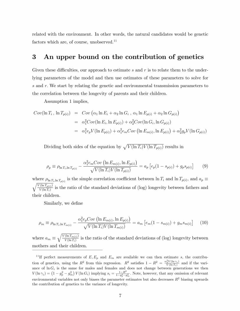
Assumption 1 implies,

Cov(lnTi ; lnTp(i)) = Cov��1 lnEi + �2 lnGi ; �1 lnEp(i) + �2 lnGp(i)

�= �21Cov(lnEi; lnEp(i)) + �

22Cov(lnGi; lnGp(i))

= �21epV (lnEp(i)) + �21emCov

�lnEm(i); lnEp(i)

�+ �22gpV (lnGp(i))

Dividing both sides of the equation bypV (lnTi)V (lnTp(i)) results in

�p � �lnTi;lnTp(i) ��21emCov

�lnEm(i); lnEp(i)

�pV (lnTi)V (lnTp(i))

= ap�ep(1� sp(i)) + gpsp(i)

�(9)

where �lnTi;lnTp(i) is the simple correlation coe¢ cient between lnTi and lnTp(i); and ap �qV (lnTp(i))

V (lnTi)is the ratio of the standard deviations of (log) longevity between fathers and

their children.

Similarly, we de�ne

�m � �lnTi;lnTm(i) ��21epCov

�lnEm(i); lnEp(i)

�pV (lnTi)V (lnTm(i))

= am�em(1� sm(i)) + gmsm(i)

�(10)

where am �q

V (lnTm(i))

V (lnTi)is the ratio of the standard deviations of (log) longevity between

mothers and their children.

11If perfect measurements of E;Ep and Em are available we can then estimate s; the contribu-

tion of genetics, using the R2 from this regression. R2 satis�es 1 � R2 = �22V (ln i)V (lnTi)

and if the vari-ance of lnGi is the same for males and females and does not change between generations we thenV (ln i) =

�1� g2p � g2m

�V (lnGi) implying si = 1�R2

1�g2p�g2m: Note, however, that any omission of relevant

environmental variables not only biases the parameter estimates but also decreases R2 biasing upwardsthe contribution of genetics to the variance of longevity.

7

Equations (9) and (10) indicate that the correlation coe¢ cient between the (log)

longevity of children and that of their parents re�ects the intergenerational transmission

coe¢ cients e and g: More precisely, assuming Cov�Em(i); lnEp(i)

�= 0; �lnTi;lnTm(i) and

�lnTi;lnTp(i) are proportional to a weighted average of the corresponding coe¢ cients e and

g with weights given by the contribution of the environment and genetics, respectively,

in the parents�generation.

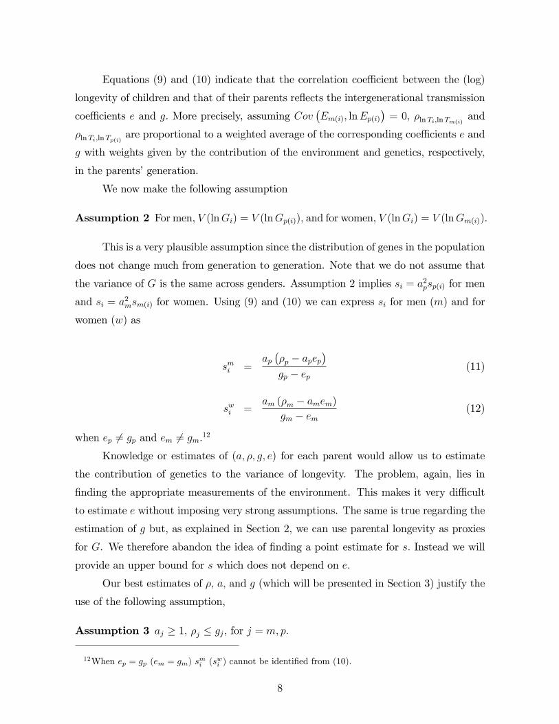
We now make the following assumption

Assumption 2 For men, V (lnGi) = V (lnGp(i)); and for women, V (lnGi) = V (lnGm(i)).

This is a very plausible assumption since the distribution of genes in the population

does not change much from generation to generation. Note that we do not assume that

the variance of G is the same across genders. Assumption 2 implies si = a2psp(i) for men

and si = a2msm(i) for women. Using (9) and (10) we can express si for men (m) and for

women (w) as

smi =ap��p � apep

�gp � ep

(11)

swi =am (�m � amem)

gm � em(12)

when ep 6= gp and em 6= gm:12

Knowledge or estimates of (a; �; g; e) for each parent would allow us to estimate

the contribution of genetics to the variance of longevity. The problem, again, lies in

�nding the appropriate measurements of the environment. This makes it very di¢ cult

to estimate e without imposing very strong assumptions. The same is true regarding the

estimation of g but, as explained in Section 2, we can use parental longevity as proxies

for G. We therefore abandon the idea of �nding a point estimate for s: Instead we will

provide an upper bound for s which does not depend on e:

Our best estimates of �; a; and g (which will be presented in Section 3) justify the

use of the following assumption,

Assumption 3 aj � 1; �j � gj; for j = m; p:

12When ep = gp (em = gm) smi (swi ) cannot be identi�ed from (10).

8

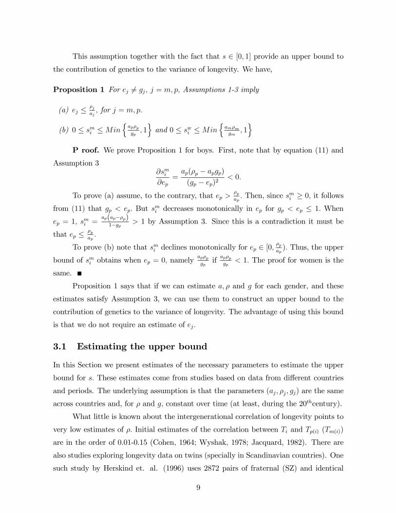
This assumption together with the fact that s 2 [0; 1] provide an upper bound tothe contribution of genetics to the variance of longevity. We have,

Proposition 1 For ej 6= gj; j = m; p; Assumptions 1-3 imply

(a) ej ��jaj; for j = m; p:

(b) 0 � smi �Minnap�pgp; 1oand 0 � swi �Min

nam�mgm

; 1o

P roof. We prove Proposition 1 for boys. First, note that by equation (11) and

Assumption 3@smi@ep

=ap(�p � apgp)(gp � ep)2

< 0:

To prove (a) assume, to the contrary, that ep >�pap: Then, since smi � 0; it follows

from (11) that gp < ep: But smi decreases monotonically in ep for gp < ep � 1: When

ep = 1; smi =ap(ap��p)1�gp > 1 by Assumption 3. Since this is a contradiction it must be

that ep ��pap:

To prove (b) note that smi declines monotonically for ep 2 [0;�pap): Thus, the upper

bound of smi obtains when ep = 0; namelyap�pgp

ifap�pgp

< 1: The proof for women is the

same.

Proposition 1 says that if we can estimate a; � and g for each gender, and these

estimates satisfy Assumption 3, we can use them to construct an upper bound to the

contribution of genetics to the variance of longevity. The advantage of using this bound

is that we do not require an estimate of ej:

3.1 Estimating the upper bound

In this Section we present estimates of the necessary parameters to estimate the upper

bound for s: These estimates come from studies based on data from di¤erent countries

and periods. The underlying assumption is that the parameters (aj; �j; gj) are the same

across countries and, for � and g; constant over time (at least, during the 20thcentury).

What little is known about the intergenerational correlation of longevity points to

very low estimates of �: Initial estimates of the correlation between Ti and Tp(i) (Tm(i))

are in the order of 0.01-0.15 (Cohen, 1964; Wyshak, 1978; Jacquard, 1982). There are

also studies exploring longevity data on twins (specially in Scandinavian countries). One

such study by Herskind et. al. (1996) uses 2872 pairs of fraternal (SZ) and identical

9

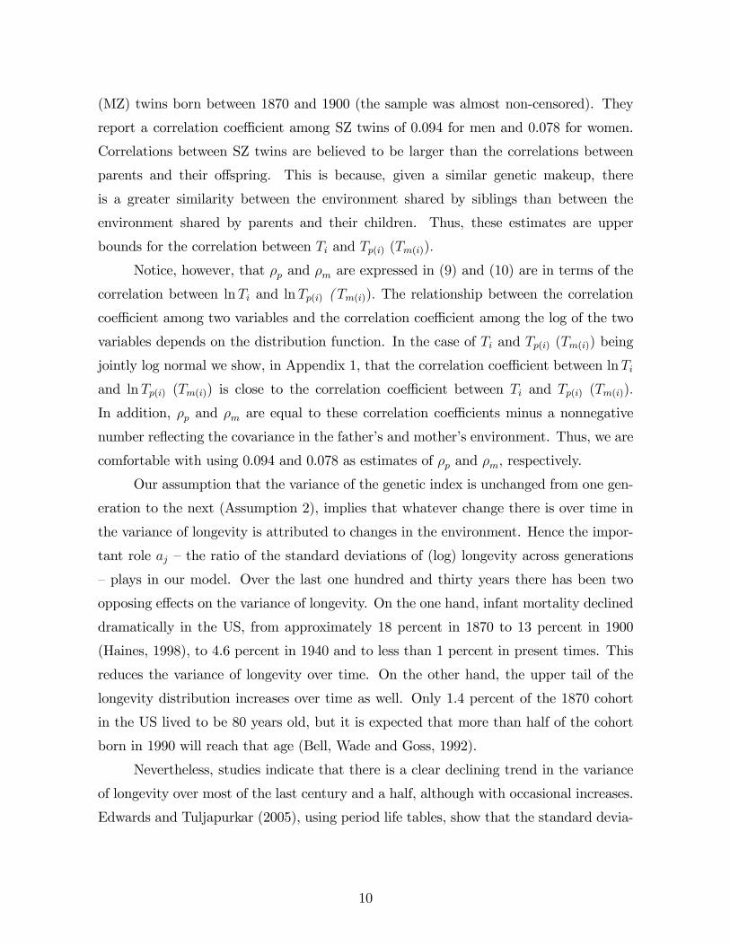
(MZ) twins born between 1870 and 1900 (the sample was almost non-censored). They

report a correlation coe¢ cient among SZ twins of 0.094 for men and 0.078 for women.

Correlations between SZ twins are believed to be larger than the correlations between

parents and their o¤spring. This is because, given a similar genetic makeup, there

is a greater similarity between the environment shared by siblings than between the

environment shared by parents and their children. Thus, these estimates are upper

bounds for the correlation between Ti and Tp(i) (Tm(i)):

Notice, however, that �p and �m are expressed in (9) and (10) are in terms of the

correlation between lnTi and lnTp(i) (Tm(i)): The relationship between the correlation

coe¢ cient among two variables and the correlation coe¢ cient among the log of the two

variables depends on the distribution function. In the case of Ti and Tp(i) (Tm(i)) being

jointly log normal we show, in Appendix 1, that the correlation coe¢ cient between lnTi

and lnTp(i) (Tm(i)) is close to the correlation coe¢ cient between Ti and Tp(i) (Tm(i)):

In addition, �p and �m are equal to these correlation coe¢ cients minus a nonnegative

number re�ecting the covariance in the father�s and mother�s environment. Thus, we are

comfortable with using 0.094 and 0.078 as estimates of �p and �m; respectively.

Our assumption that the variance of the genetic index is unchanged from one gen-

eration to the next (Assumption 2), implies that whatever change there is over time in

the variance of longevity is attributed to changes in the environment. Hence the impor-

tant role aj �the ratio of the standard deviations of (log) longevity across generations

�plays in our model. Over the last one hundred and thirty years there has been two

opposing e¤ects on the variance of longevity. On the one hand, infant mortality declined

dramatically in the US, from approximately 18 percent in 1870 to 13 percent in 1900

(Haines, 1998), to 4.6 percent in 1940 and to less than 1 percent in present times. This

reduces the variance of longevity over time. On the other hand, the upper tail of the

longevity distribution increases over time as well. Only 1.4 percent of the 1870 cohort

in the US lived to be 80 years old, but it is expected that more than half of the cohort

born in 1990 will reach that age (Bell, Wade and Goss, 1992).

Nevertheless, studies indicate that there is a clear declining trend in the variance

of longevity over most of the last century and a half, although with occasional increases.

Edwards and Tuljapurkar (2005), using period life tables, show that the standard devia-

10

tion in life span have declined across industrialized countries since 1960.13 This implies

aj � 1 but perhaps not much larger than 1:We estimated the variance of (log) longevityfor four cohorts of individuals born in the U.S. in 1870, 1880, 1900 and 1910. We use

data on age-speci�c hazards given by Haines (1998) to back up the probability density

function of T and use it to estimate the variance of lnT by gender and year of birth.

Assuming that parents and children are born 30 years apart we use the estimated vari-

ances to estimate a for the 1900 and 1910 generations (details are in Appendix 2). Table

1 shows the results. Notice that after 1880 the variance is declining for both men and

women. For each gender, we averaged the standard deviations in 1870 and 1880 and

divided them by the 1990-1910 average standard deviation of all children. This gives our

estimate of ap and am which is 1.16 for fathers and mothers.

The remaining parameters needed to estimate the bound are gp and gm: These

are much more di¢ cult parameters to estimate since they relate to the interrelationship

between the unobservable genetic factors, Gi; Gp(i) and Gm(i): This is where data on

parental longevity become useful since, as argued in Section 2, parental longevity can

serve as a proxy for genetic factors.

We therefore proceed to estimate g using a newly assembled longevity data set

for Israel which matches individuals born during 1901-1909 to their parents (born in

the 19th century). The data are based on records from the o¢ cial Population Registry

of the State of Israel. A record in the Registry has the individual�s name and identity

number as well his or her parents�names and, in some cases, their identity numbers.

When available, the parents�identity number is used to access the parents�records at

the Registry. The Registry provides information on the date of birth and on the date

of death if the person died before October 31, 2008, the last update of the Registry. It

follows that the way the Registry is organized allows us, in principle, to match children

to parents and obtain the children�s and parents�dates of birth and death.

In Appendix 3 we explain the details of the matching algorithm. We matched

individuals to their fathers; the matching to mothers was problematic and is therefore

not used in this paper. We can then only estimate gp: We focus on individuals born in

the �rst decade of the 20th century to avoid, as much as possible, censoring of Ti: Indeed,

131960 is the inital date in their study. The countries are Canada, Britain, Denmark, France, Japan,Sweden, and the United States.

11

only 0.7 percent of the individuals in this sample are censored.14 The sample consists of

640 males and 179 females born between 1901-1909 who were successfully matched to

their father.15

We estimate equation (8) by OLS for men and women separately using country

of birth, year of birth, cohort of immigration, and country of father�s birth as proxies

for Ei and Ep(i); but omitting lnTm(i) from the regressions. Results appear in Table 2.

The estimates of gp hover around 0.33 for males and around 0.26 for females and are

statistically signi�cant for men but not that signi�cant for women because of the smaller

number of observations. The inclusion of the environmental covariates does not a¤ect

much the estimate of g except, perhaps, for father�s county of birth whose inclusion

increases the estimated gp from about 0.18 to 0.26 in the women�s regressions.

Our estimates of g are in the order of magnitude of what one would expect. In the

�twin studies� literature the usual correlation between the genetic factors of fraternal

(SZ) twins is between 1/4 to 1/2 of the correlation among identical (MZ) twins (see a

critical survey by Goldberger, 2005). Since the genetic correlation between MZ twins

is close to unity and the correlation between the genetic factors of parents and their

children, denoted by �Gp ; is largely the same as the correlation between SZ twins, we

would expect the correlation between parents and children to be also between 1=4 and

1=2. The link between gp and �Gp is given by using equation (2) and Assumption 2 to

express the correlation between fathers and children�s genes as a function of gp (and gm);

gp = �Gp � gm

Cov(lnGp; lnGm)

V (lnGp):

Since Cov(lnGp; lnGm) is probably positive but small we expect gp to be at the

lower end of the interval between 1/4 and 1/2. In fact, assume that gp = gm = g; which is

not far from our estimates, and that V (lnGp) = V (lnGm): Then, g =�Gp

1+�Gpm, where �Gpm

is the correlation between the genetic factors of father and mother. Since �Gpm is smaller

than �Gp we have that g is between�Gp1+�Gp

(when �Gpm = �Gp ) and �Gp (when �

Gpm = 0): If

�Gp = 3=8 �the midpoint between 1/4 and 1/2 �then g 2 [0:273; 0:375]:

14As opposed to 10.3 percent among those born between 1910 and 1919, and 38.3 percent amongthose born in 1920-1929. Including the 6 censored individuals in the regressions �essentially assumingthat they died at the end of the sample period�does not change the results.

15We do not include the year 1900 because there is an abnormal number of individuals born in thatyear suggesting that people reported �1900�as their date of birth when the true date was, presumably,unknown.

12

Our main econometric concern is that the OLS estimate of gp may be biased

upward since this will make the upper boundMinnap�pgp; 1osmaller than what it actually

is. There are certainly reasons for concern because several variables are omitted when

estimating (8): Note, however, that because lnTm(i) = �1 lnEm(i) + �2 lnGm(i); equation

(8) can be rewritten as

lnTi = gp lnTp(i) + �1 lnEi � �1gp lnEp(i) + �2gm lnGm(i) + �2 ln i (13)

and we use this formulation to examine the bias in the OLS estimator of gp:

First, note that Assumption 1 implies that ln i is not correlated with father�s

longevity. Moreover, if the mother�s genes are not correlated with those of the father,

then lnTp(i) is uncorrelated with the omitted term �2gm lnGm(i): However, if there is

assortative mating and more genetically similar individuals get married, then we would

expectGm(i) andGp(i) to be positively correlated . This would imply a positive correlation

between Tp(i) and Gm(i) and an upward biased estimator of gp:

Second, we mentioned above that it is intrinsically impossible to de�ne and to

measure Ei and Ep(i): We use a set of proxies for them but it is likely that we omit

other determinants of lnEi and lnEp(i) that could be correlated with lnTp: Suppose that

we omit lnEp(i) from the regression. Since Ep(i) is positively correlated with lnTp �see

equation (4) �its omission biases the estimation of gp downwards (because of the negative

coe¢ cient on lnEp(i)). This can be seen very clearly in the women�s panel where adding

father�s country of birth increases the estimated gp:

Finally, we analyze the e¤ect of having insu¢ cient proxies for the environment.

Linearly projecting lnE on a set of proxy variables z = (z1; z2) we can write lnE =

z1�1+z2�2+r with Cov(z; r) = 0:We assume Cov(lnTp; r) = 0 so that, given z; father�s

longevity is not correlated with the (residual) environment. When z2 is omitted from

the regression and is correlated with lnTp; the OLS estimator of gp will be biased. The

direction of the bias depends on the sign of the correlation between lnTp and each element

in z2 and on the sign of �2:When the omitted factors have a positive e¤ect on lnE, �2 > 0;

they are also likely to be positively correlated with lnTp and therefore Cov(lnTp; z2�2) >

0: Thus, the omission of environmental variables is likely to overestimate gp:16 This

upward bias is apparently small since the estimated gp is not much a¤ected by the

16When the omitted factors, e.g., pollution, have a negative e¤ect on lnE, �2 < 0; they are also likelyto be negatively correlated with lnTp and therefore Cov(lnTp; z2�2) > 0 as well.

13

inclusion or omission of the various environmental controls. In fact, we would not expect

a large bias from omitting environmental factors common to parents and their children

because, as we will show below, the coe¢ cients ep and em are very small. The remaining

part of lnE; ln �; is uncorrelated with lnTp(i):

In sum, although we omit several regressors when estimating (13), we have shown

that the bias in the estimator of gp can go in di¤erent directions. Because our estimates

of gp are in the order of magnitude suggested by the �twin studies�literature, the various

sources of bias appear to be cancelling each other.

Lastly, our sample is truncated (from below) because it only includes individuals

that were alive by January 1, 1949. That is, the age at death in our sample of individuals

is above 41 years of age (= 1949�1909). Assuming that the error term in (13) is normallydistributed we can account for this truncation by estimating the parameters by maximum

likelihood.17 Results appear in Table 3. Of course, the normality assumption may not

be appropriate but it is nevertheless comforting to observe that the estimates of gp are

almost identical to the OLS estimates that ignore the truncation.18

In Table 4 we combine these estimates to calculate the upper bound for the genetic

contribution to the variance of (log) longevity. Using the estimated g0ps from the most

inclusive speci�cation (column (4)) and the other estimates reported above, we �nd that

s is bounded by 0.32 for both men and women (assuming gp = gm). This means that

the contribution of the environment is at least 68 percent.

Part a of Proposition 1 has another important implication. It states that the

transmission parameters of the environment, ep and em; are bounded by�a: Given the

estimated parameters, ep and em are very small: less than 0.07-0.08. Thus, most of

the variance of lnE is due to the variance of ln �: In other words, most of the variance

17Each individual is truncated from below by ci where ci equals the di¤erence (in days) betweenJanuary 1, 1949 and the date of the individual�s birth if he or she was born in Israel or immigratedbefore 1.1.1949, and the date of immigration if he or she immigrated after 1.1.1949.

18The age at death of the fathers is truncated from below at an even higher value. In our sample,the observations include only fathers that died after reaching 60 years of age (fathers born around 1890and dying in 1949-50). Truncation on the explanatory variable is not a problem since our estimatesare conditional on the observed data. Our extrapolation of the estimated g0ps to the whole populationis based on the implicit assumption that gp does not depend on the age of father�s age. This type ofassumption is prevalent in most empirical work.The truncation of T and Tp means that we cannot use the sample variances and covariances to

estimate � and a since these are very much a¤ected by the truncation. Adjusting for truncation requiresdistributional form assumptions which are, at best, educated guesses.

14

in longevity is due to non-inherited environmental factors. Note that this is a direct

implication of Proposition 1 and of the estimates of a and � and is not related to the

measurement of the environment.19 Put di¤erently, although longevity is a¤ected by

genetics and parental environment, most of the observed variation in longevity cannot

be explained by either.20

4 Conclusions

In the past 150 years, the average life span has nearly doubled. Initially, the main reason

for this dramatic increase was the reduction in infant mortality (in the US, from around

18 percent in the 1870s to about less than 1 percent today). Since the 1940s, with

the discovery and dissemination of antibiotics to treat infectious diseases, improvements

in medicine have been responsible for the prolongation of life. In recent decades, new

procedures for treating heart diseases contributed to the continuing decline in mortality

rates at older ages (in the US, only 10 percent of the population lived to be 80 years in

the mid 19th century while today more than 53 percent reach this age).

As argued by Christensen et. al. (2006), this large change on such a short time

on an evolutionary timescale, indicates the dominant role of non-genetic factors in de-

termining longevity. This is consistent with our �nding that environment is responsible

for at least two thirds of the variance of (log) longevity. Moreover, we interpret genetics

in a broad sense (G captures the indirect e¤ect, via the environment, on longevity) and

therefore the contribution of the �pure�genetic component is likely to be much smaller

than one third.

Perhaps more surprising is our �nding that parental socio-economic status is less

important in determining longevity than the non-inherited component of environment.

This is seen in the small values of the transmission parameters ep and em which are a

direct result of the low correlation in the longevity of parents and their children reported

in the literature. Thus, most of the variance in (log) longevity is not inherited from

parents. This has important implications for public policy to the extent that policy can

19This �nding also accords well with Smith�s (1999) observation that �the vast majority of variationin individual health is within socioeconomic groups, not between them�.

20One quali�cation to this statement is that it we use data from developed countries and thereforeour empirical analysis applies to such countries.

15

a¤ect the environment.

Finally, the paper presents a structural interpretation of the variance decomposition

used in much of the behavioral genetic literature. It is this structure, and knowledge

of its parameters, that allows us to infer the contribution of genetics and the role of

inherited and non-inherited factors to longevity.

16

References

[1] Bell Felicitie, Alice H. Wade and Stephen C. Goss, �Life Tables for the United States

Social Security Area 1900-2080,�U. S. Department of Health and Human Services,

1992 Pub. No. 11-11536.

[2] Black, Sandra, Paul Devereux and Kjell Salvanes, �Like father, like son? A note on

the intergenerational transmission of IQ scores�, NBER WP 14274, August 2008,

http://papers.nber.org/papers/W14274.

[3] Case Anne, Angela Fertig and Christina Paxson. �The Lasting Impact of Childhood

Health and Circumstance�, Journal of Health Economics 2005 24(1) pp. 365-389.

[4] Case Anne, Darren Lubotsky and Christina Paxson. �Economic Status and Health

in Childhood: The Origins of the Gradient�, The American Economic Review 2002,

92(5): pp. 1308-1334.

[5] Christensen, K., T.E. Johnson and J.W. Vaupel, �The quest for genetic determi-

nants of human longevity: challenges and insights�, Nature Review Genetics, 7,

June 2006, 436-448.

[6] Cohen, H.B., �Family patterns of mortality and life span�, The Quarterly Review

of Biology, 39, 1964, 130�181.

[7] Currie Janet and Enrico Moretti. �Biology as Destiny? Short- and Long-Run De-

terminants of Intergenerational Transmission of Birth Weight�, Journal of Labor

Economics, 2007, 25(2): pp. 231-264.

[8] Cutler, Deaton and Lleras-Muney, 2006 �The Determinants of Mortality�, The Jour-

nal of Economic Perspectives, 20(3), pp. 97-120.

[9] Goldberger A. S., and C. F. Manski, �The Bell Curve: Intelligence and Class Struc-

ture in American Life. by Richard J. Herrnstein and Charles Murray,�Journal of

Economic Literature, 1995, 33(2), 762-776.

[10] Goldberger A. S., �Structural Equation Models in Human Behavior Genetics�, chap-

ter 2 in Identi�cation and Inference for Econometric Models: Essays in Honor of

17

Thomas Rothenberg, edited by Donald W. K. Andrews, James H. Stock, Cambridge,

UK: Cambridge University Press, 2005.

[11] Haines, Michael. R. (1998): �Estimated Life Table for the United States, 1850�

1910,�Historical Methods, 31, 149�167.

[12] Herrnstein R. J. and C. Murray, The Bell Curve: Intelligence and Class Structure

in American Life. New-York, Free press,1994.

[13] Herskind A. M., M. McGue, N. V. Holm, T. I. A. Sorensen, B. Harvald, J.W. Vaupel,

�The heritability of human longevity: a population-based study of 2872 Danish twin

pairs born 1870-1900�, Human Genetics, 97, 1996, 319-323.

[14] Hjelmborg Jacob vB. , Ivan Iachine, Axel Skytthe, James W. Vaupel, Matt McGue,

Markku Koskenvuo, Jaakko Kaprio, Nancy L. Pedersen and Kaare Christensen

(2006), �Genetic in�uence on human lifespan and longevity�, Human Genetics 119,

312�321.

[15] Jacquard, �Heretability and Human Longevity,� pages 303-313 in Biological and

Social Aspects of Mortality and the Length of Life edited by S. H. Preston, Ordina,

Liege, Belgium, 1982.

[16] Marenberg Marjorie E., Neil Risch, Lisa F. Berkman, Birgitta Floderus, and Ulf de

Faire (1994), �Genetic Susceptibility to Death from Coronary Heart Disease in a

Study of Twins�, New England Journal of Medicine, 330(15), 1041-1046.

[17] Osler, M., Petersen, L., Prescott, E., Teasdale, T. W, Sorensen, T. I A (2006),

�Genetic and environmental in�uences on the relation between parental social class

and mortality�, International Journal of Epidemiology 35, 1272-1277.

[18] Plomin, Robert, John C. DeFries, and David W. Fulker, Nature And Nurture During

Infancy And Early Childhood, (Cambridge, MA: Cambridge University Press, 1988).

[19] Plug, Erik, and Wim Vijverberg, �Schooling, Family Background and Adoption: Is

it Nature or is it Nurture?,�Journal of Political Economy, CXI, 2003, 611�641.

18

[20] Sacerdote B., �How large are the e¤ects from changes in family environment?

A study from the Korean American Adoptees,�Quarterly Journal of Economics,

CXXII, 2007, 119-157.

[21] Sacerdote B., �The Nature and Nurture of Economic Outcomes,�American Eco-

nomic Review, 2002, 92(2), 344�348.

[22] Smith, J. P., �Healthy bodies and thick wallets: the dual relation between health

and economic status�, Journal of Economic Perspectives, 13, 1999, 145�166.

[23] Solon, Gary, �Intergenerational Mobility in the Labor Market,�in Orley C. Ashen-

felter and David Card, eds., Handbook of labor economics, Vol. 3A. Amsterdam:

North-Holland, 1999, 1761-1800.

[24] Solon, Gary, �Intergenerational Income Mobility,�in Steven Durlauf and Lawrence

Blume (eds.), The New Palgrave Dictionary of Economics, 2nd edition, London:

Macmillan, 2008.

[25] Sorensen TI , GG Nielsen, PK Andersen, and TWTeasdale (1988), �Genetic and en-

vironmental in�uences on premature death in adult adoptees�, New England Journal

of Medicine, Volume 318:727-732, March 24, Number 12.

[26] Wyshak Grace, �Fertility and Longevity in Twins, sibs, and Parents of Twins,�

Social Biology, 25: 315-330.

19

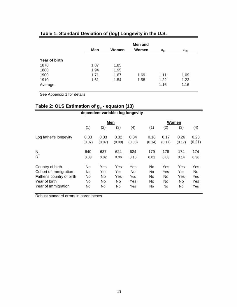
Table 1: Standard Deviation of (log) Longevity in the U.S.

Men andMen Women Women ap am

Year of birth1870 1.87 1.851880 1.94 1.951900 1.71 1.67 1.69 1.11 1.091910 1.61 1.54 1.58 1.22 1.23Average 1.16 1.16

See Appendix 1 for details

Table 2: OLS Estimation of gp ­ equaton (13)

(1) (2) (3) (4) (1) (2) (3) (4)

Log father's longevity 0.33 0.33 0.32 0.34 0.18 0.17 0.26 0.28(0.07) (0.07) (0.08) (0.08) (0.14) (0.17) (0.17) (0.21)

N 640 637 624 624 179 178 174 174R2 0.03 0.02 0.06 0.16 0.01 0.08 0.14 0.36

Country of birth No Yes Yes Yes No Yes Yes YesCohort of Immigration No Yes Yes No No Yes Yes NoFather's country of birth No No Yes Yes No No Yes YesYear of birth No No No Yes No No No YesYear of Immigration No No No Yes No No No Yes

Robust standard errors in parentheses

dependent variable: log longevity

Men Women

20

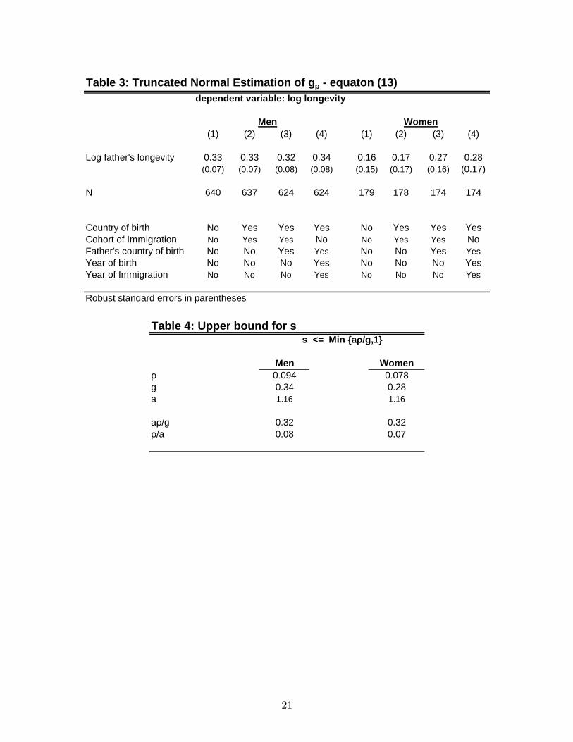
Table 3: Truncated Normal Estimation of gp ­ equaton (13)

(1) (2) (3) (4) (1) (2) (3) (4)

Log father's longevity 0.33 0.33 0.32 0.34 0.16 0.17 0.27 0.28(0.07) (0.07) (0.08) (0.08) (0.15) (0.17) (0.16) (0.17)

N 640 637 624 624 179 178 174 174

Country of birth No Yes Yes Yes No Yes Yes YesCohort of Immigration No Yes Yes No No Yes Yes NoFather's country of birth No No Yes Yes No No Yes YesYear of birth No No No Yes No No No YesYear of Immigration No No No Yes No No No Yes

Robust standard errors in parentheses

dependent variable: log longevity

Men Women

Table 4: Upper bound for s

Men Womenρ 0.094 0.078g 0.34 0.28a 1.16 1.16

aρ/g 0.32 0.32ρ/a 0.08 0.07

s  <=  Min {aρ/g,1}

21

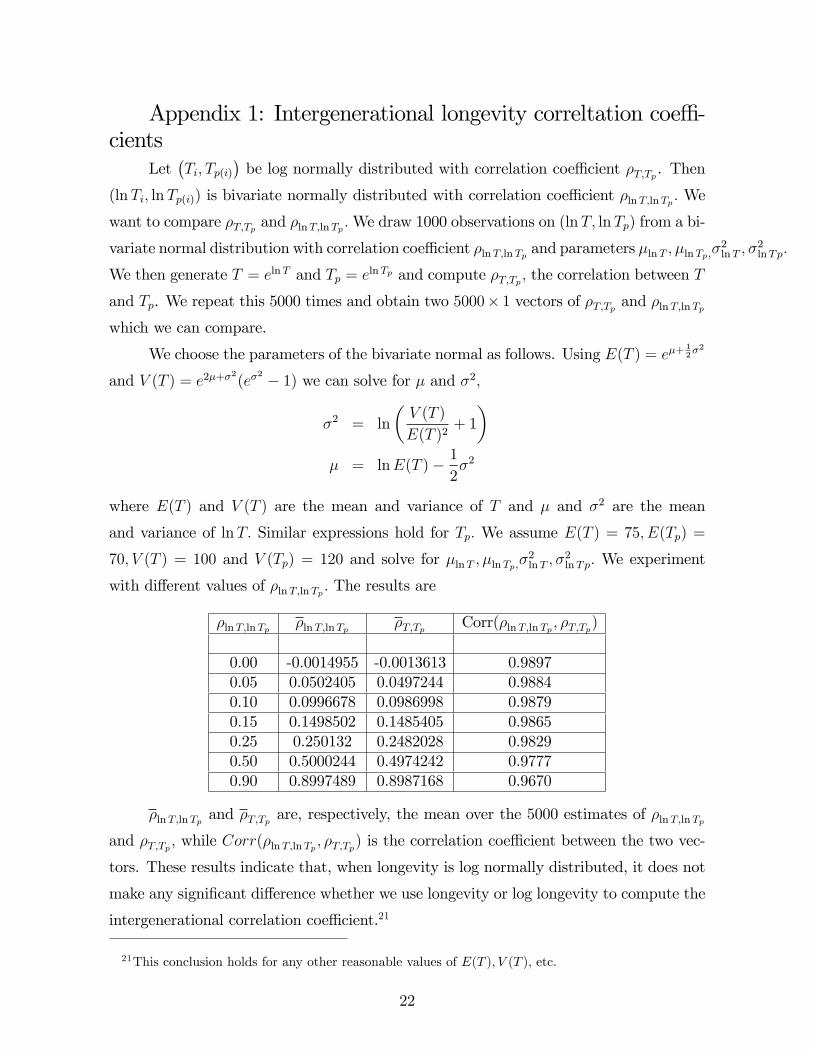
Appendix 1: Intergenerational longevity correltation coe¢ -cients

Let�Ti; Tp(i)

�be log normally distributed with correlation coe¢ cient �T;Tp . Then

(lnTi; lnTp(i)) is bivariate normally distributed with correlation coe¢ cient �lnT;lnTp : We

want to compare �T;Tp and �lnT;lnTp :We draw 1000 observations on (lnT; lnTp) from a bi-

variate normal distribution with correlation coe¢ cient �lnT;lnTp and parameters �lnT ; �lnTp;�2lnT ; �

2lnTp:

We then generate T = elnT and Tp = elnTp and compute �T;Tp ; the correlation between T

and Tp. We repeat this 5000 times and obtain two 5000� 1 vectors of �T;Tp and �lnT;lnTpwhich we can compare.

We choose the parameters of the bivariate normal as follows. Using E(T ) = e�+12�2

and V (T ) = e2�+�2(e�

2 � 1) we can solve for � and �2;

�2 = ln

�V (T )

E(T )2+ 1

�� = lnE(T )� 1

2�2

where E(T ) and V (T ) are the mean and variance of T and � and �2 are the mean

and variance of lnT: Similar expressions hold for Tp: We assume E(T ) = 75; E(Tp) =

70; V (T ) = 100 and V (Tp) = 120 and solve for �lnT ; �lnTp;�2lnT ; �

2lnTp: We experiment

with di¤erent values of �lnT;lnTp : The results are

�lnT;lnTp �lnT;lnTp �T;Tp Corr(�lnT;lnTp ; �T;Tp)

0.00 -0.0014955 -0.0013613 0.98970.05 0.0502405 0.0497244 0.98840.10 0.0996678 0.0986998 0.98790.15 0.1498502 0.1485405 0.98650.25 0.250132 0.2482028 0.98290.50 0.5000244 0.4974242 0.97770.90 0.8997489 0.8987168 0.9670

�lnT;lnTp and �T;Tp are, respectively, the mean over the 5000 estimates of �lnT;lnTpand �T;Tp ; while Corr(�lnT;lnTp ; �T;Tp) is the correlation coe¢ cient between the two vec-

tors. These results indicate that, when longevity is log normally distributed, it does not

make any signi�cant di¤erence whether we use longevity or log longevity to compute the

intergenerational correlation coe¢ cient.21

21This conclusion holds for any other reasonable values of E(T ); V (T ); etc.

22

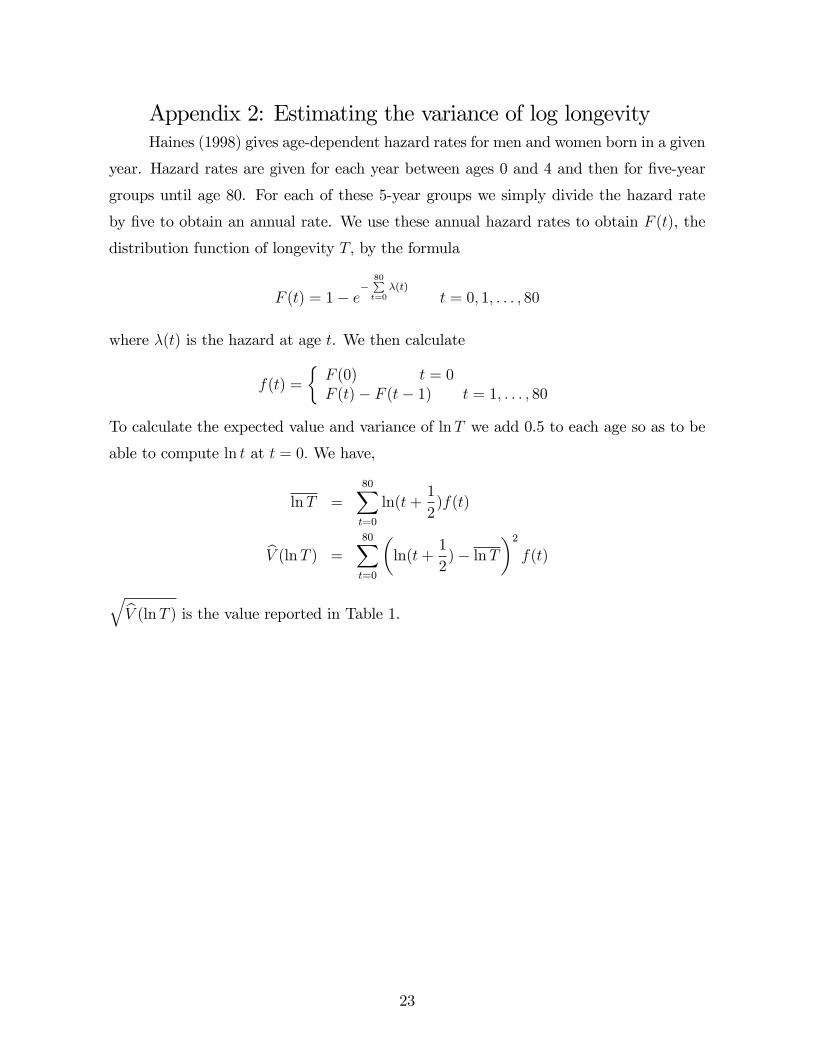
Appendix 2: Estimating the variance of log longevityHaines (1998) gives age-dependent hazard rates for men and women born in a given

year. Hazard rates are given for each year between ages 0 and 4 and then for �ve-year

groups until age 80. For each of these 5-year groups we simply divide the hazard rate

by �ve to obtain an annual rate. We use these annual hazard rates to obtain F (t), the

distribution function of longevity T; by the formula

F (t) = 1� e�

80Pt=0

�(t)t = 0; 1; : : : ; 80

where �(t) is the hazard at age t. We then calculate

f(t) =

�F (0) t = 0F (t)� F (t� 1) t = 1; : : : ; 80

To calculate the expected value and variance of lnT we add 0.5 to each age so as to be

able to compute ln t at t = 0: We have,

lnT =80Xt=0

ln(t+1

2)f(t)

bV (lnT ) =80Xt=0

�ln(t+

1

2)� lnT

�2f(t)

qbV (lnT ) is the value reported in Table 1.

23

Appendix 3: Construction of the longevity dataOur data are based on records from the o¢ cial Population Registry of the State of

Israel. A record in the Registry has the individual�s name and identity number as well

his or her parents�names and, in some cases, their identity numbers. When available,

the parents�identity number is used to access the parents�records at the Registry. The

Registry provides information on the date of birth and on the date of death if the person

died before October 31, 2008, the last update of the Registry. The Registry does not

record the cause of death. It follows that the way the Registry is organized allows us, in

principle, to match children to parents and obtain the children�s and parents�dates of

birth and death.

Using the available identity numbers we matched the 228,808 individuals born in

1901-1909 to their fathers. The number of matches is very low �only 21!� and it is

due to the fact that records of the older cohorts are incomplete. Fortunately, the Israeli

Population Registry has a unique feature that allows us to generate many more matches

than those available directly from the Registry.

The Registry was established in 1948 with the creation of the State of Israel.

Surveyors went house by house and recorded demographic data of each person in the

household (children and adults). In particular, for each individual they recorded the

names (�rst and last) of their parents and assigned consecutive identity numbers to

all household members. Furthermore, families who immigrated to Israel following its

establishment in 1948 were also assigned consecutive identity numbers. Thus, the identity

numbers of most of the Jewish population in Israel, who were born in Israel before 1948 or

immigrated to Israel after 1948, are bundled together by families. We exploit this feature

to generate additional matches between children and their parents. The algorithm that

generates these matches (to fathers) works as follows:

1. Sort the Population Registry by ascending id number.

2. For each record i in the Registry, select the 10 records preceding and the 10 records

following record i:

3. Among these 20 records, select those that are males.

4. Among these records, select those with a �rst and last name equal to the father�s

name in record i:

24

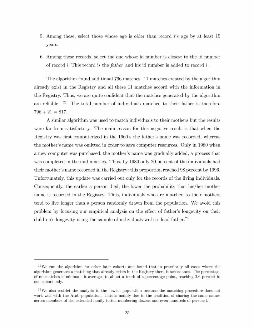
5. Among these, select those whose age is older than record i0s age by at least 15

years.

6. Among these records, select the one whose id number is closest to the id number

of record i: This record is the father and his id number is added to record i:

The algorithm found additional 796 matches. 11 matches created by the algorithm

already exist in the Registry and all these 11 matches accord with the information in

the Registry. Thus, we are quite con�dent that the matches generated by the algorithm

are reliable. 22 The total number of individuals matched to their father is therefore

796 + 21 = 817:

A similar algorithm was used to match individuals to their mothers but the results

were far from satisfactory. The main reason for this negative result is that when the

Registry was �rst computerized in the 1960�s the father�s name was recorded, whereas

the mother�s name was omitted in order to save computer resources. Only in 1980 when

a new computer was purchased, the mother�s name was gradually added, a process that

was completed in the mid nineties. Thus, by 1980 only 20 percent of the individuals had

their mother�s name recorded in the Registry; this proportion reached 98 percent by 1996.

Unfortunately, this update was carried out only for the records of the living individuals.

Consequently, the earlier a person died, the lower the probability that his/her mother

name is recorded in the Registry. Thus, individuals who are matched to their mothers

tend to live longer than a person randomly drawn from the population. We avoid this

problem by focusing our empirical analysis on the e¤ect of father�s longevity on their

children�s longevity using the sample of individuals with a dead father.23

22We run the algorithm for other later cohorts and found that in practically all cases where thealgorithm generates a matching that already exists in the Registry there is accordance. The percentageof mismatches is minimal: it averages to about a tenth of a percentage point, reaching 2.6 percent inone cohort only.

23We also restrict the analysis to the Jewish population because the matching procedure does notwork well with the Arab population. This is mainly due to the tradition of sharing the same namesacross members of the extended family (often numbering dozens and even hundreds of persons).

25