Embed Size (px)
Citation preview

1
Natural Gas Supply
Francis O’Sullivan, Ph.D.
May 25th, 2011
EPRI Global Climate Change Research Seminar

2
A review of 2009 U.S. primary energy consumption by source and sector reveals the broad systemic importance of natural gas
Source: EIA
Supply Sources
7.7Renewables
Nuclear8.3
35.3Petroleum
19.7Coal
Electric Power
Industrial
10.6
38.3
18.8
27.0
94.6 Quads
Residential &Commercial
Transport
23.4Natural Gas
Demand Sectors
72%
22%
5%1%
3%32%
35%30%
7%<1%
93%
12%26%
9%
53%
100%
48%1%
18%
11%
22%
17%76%
1%7%
41%
7%11%
40%
94%
3%3%
2

3
The global natural gas resource

Working D
raft -Last Modified 5/4/2010 6:23:07 PM
Printed
4
Middle East
Russia
United States
Central Asia
Africa
Latin America
W. Europe
Canada
Dynamic Asia
Brazil
Rest of E. Asia
Oceania
China
Mexico
India
6,0000 1,000 2,000 3,000 4,000 5,000
There is a lot of gas in the world, ~16,000 Tcf – but these resources are highly concentrated
Breakdown of the total global remaining recoverable gas resources by EPPA region Tcf of Gas
Proved ReservesReserve GrowthUnconventional Resources**Yet-to-Find Resource (Mean)P90YTF
P10 YTFGlobal gas
consumption in 2009 was ~107
Tcf
Source: MIT Gas Supply Team analysis

55
0.00
2.00
4.00
6.00
8.00
10.00
12.00
14.00
16.00
18.00
20.00
0 4,000 8,000 12,000 16,000 20,000
Example LNG value chain costs incurred during gas delivery$/MMBtu**
Liquefaction $2.15
Shipping $1.25
Regasification $0.70
Total $4.10
Volumetric uncertainty around mean of 16,200 Tcf
P9012,500
P1020,600
Global breakeven gas price$/MMBtu*
* Cost curves based on 2007 cost bases. North America cost represent wellhead breakeven costs. All curves for regions outside North America represent breakeven costs at export point. Cost curves calculated using 10% real discount rate
** Assumes two 4MMT LNG trains with ~6,000 mile one-way delivery run Source: MIT Gas Supply Team analysis, ICF Hydrocarbon Supply Model, Jensen and Associates
Much of this resource can be developed at low cost – but long distance transportation costs will significantly increase its delivered cost
P90MeanP10

6Source:“An assessment of world hydrocarbon resources”, H-H Rogner, Annu. Rev. Energy Environ., 1997
Breakdown of global unconventional GIIP by region and typeTcf of gas
Sub-Saharan
Africa
Middle East and
North Africa
Former Soviet Union
Central and
Eastern Europe
South Asia
Latin America
Western Europe
Other Asia
Pacific
Pacific (OECD)
Central Asia and
China
North America
6
Early analysis suggested that there may be very extensive global unconventional resources
9,000
8,000
7,000
6,000
5,000
4,000
3,000
2,000
1,000
TightShaleCBM

7Source: World Shale Gas Resources: An Initial Assessment of 14 Regions Outside the United States, ARI 2011 7
A recent global assessment of shale gas suggests at least 6,000 Tcf of recoverable resources, with over 1,200 Tcf located in China
Argentina 774 TcfBrazil 226 Tcf
Poland 187 TcfFrance 180 Tcf
South Africa 485 TcfLibya 290 Tcf
China 1,275 TcfIndia 63 Tcf
396
1404
1042
624
1225
0
300
600
900
1200
1500
Australia Asia Africa Europe South America
Breakdown of global recoverable shale gas resources by region Tcf of gas
Top two shale gas resource holders by region
Study only assessed 31 countries – Future work expected to increase the
resource estimate substantially

8
Gas dynamics in the United States

The past 5 years have seen a dramatic increase in both proved reserves and more importantly in the technically recoverable resource – All due to shale
9
0
500
1000
1500
2000
2500
3000
3500
4000+80%Resources
Proved Reserves
Cumulative production
Illustration of US gas production, reserve and resource dynamics from ’90 to ‘10Tcf of gas
184 204 245 273
1218 1290 1219 1219
616827
0
500
1000
1500
2000
2500
NPC 2003 PGC 2006 PGC 2008 EIA 2010
Shale Resources
Non-Shale Resources
Proved Reserves
Illustration of the change in recoverable resource assessment by gas type over the past decade1
Tcf of gas
1. EIA 2010 assessment based on 2008 PGC assessment with updated estimates of technically recoverable shale gas volumesSource: NPC data, PGC data, EIA data

The emergence of shale gas as a recoverable resource is illustrated in the production dynamics – Shale gas is driving U.S. production growth
10
0
5
10
15
20
25
2000 2002 2004 2006 2008 2010
55%41%
16%
11%
22%
25%
14%
7% 8%
2000 2009
Breakdown of US gas production by type1
Tcf of gasComparison of production by type – ’00 vs. ‘091
Percent of total production
20.5 Tcf 22.1 Tcf
Coal Bed Methane
Shale
Tight
Associated
Conventional
• In 2000, 14.6 Tcf of conventional gas was produced, representing 71% of total US marketable production
• By 2009, conventional production fell to 11.6 Tcf, or just over 50% of total production
• In the same period shale gas output grew from almost nothing to over 3.5 Tcf, and is now the only production segment that is growing
1. United States production figures represent marketable production, and so exclude gas produced in Alaska, which is subsequently reinjected Source: HPDI commercial production database
11
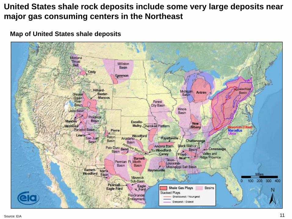
United States shale rock deposits include some very large deposits near major gas consuming centers in the Northeast
Map of United States shale deposits
Source: EIA

12
NPC ’03
EIA ’07
ICF ’08
PGC ’09
ICF ’09
2002 2003 2004 2005 2006 2007 2008 2009 2010
Year
The focus on shale gas has led to large increases in mean resource estimates; however, these mean estimates are accompanied by wide error bars
* Mean volumes represent the “most likely” estimates reported by the PGC and can be aggregated by arithmetic addition to yield an aggregated mean estimate of shale gas resources in the United States. The per basin min and max numbers reported here assume perfect statistical correlation within basins
** US min and max totals are for illustrative purposes only, and are calculated by direct addition of volumes, not statistical aggregation Source: Various commercial and institutional resource assessments
Total Mean Estimate:
Min
616
Mean Max
Fort Worth Basin:Barnett Shale 25 59 100
Arkoma Basin:Fayetteville/Woodford 70 110 146
E. TX & LA Basin:Haynesville Shale 60 112 182
Appalachian Basin:Marcellus/Ohio/Utica Shale 92 227 549
Anadarko/Permian Basins:Barnett/Woodford Shales 3 6 16
Other Basins: 51 100 224
Comparison of mean estimates of shale gas resources in the United States Tcf of Gas
Recent focus on assessing the shale gas potential in the U.S. has resulted in dramatic increases in resource estimates
Breakdown of the PGC 2009 shale gas resource estimates by major U.S. shale play*Tcf of Gas
301** 1217**

1313
0.00
5.00
10.00
15.00
20.00
25.00
30.00
35.00
40.00
0 500 1,000 1,500 2,000 2,500 3,000
0.00
5.00
10.00
15.00
20.00
25.00
30.00
35.00
40.00
0 200 400 600 800 1,000
The US gas supply curves reveal large volumes of relatively cheap gas –Remarkably, shale gas is the most important source of low cost resource
United States breakeven gas price$/MMBtu*
Breakdown of United States breakeven gas price by resource type$/MMBtu*
* Cost curves calculated using 2007 cost bases. U.S. costs represent wellhead breakeven costs. Cost curves calculated assuming 10% real discount rate Source: MIT Gas Supply Team analysis, ICF Hydrocarbon Supply Model, Data strictly for illustrative purposes only
P90MeanP10
ConventionalShaleTightCBM

IP rate variability is a major issue with shales – In the Barnett, IP rates vary by 3X between P20 and P80 performance, while other shales display even greater variability
14
Pro
babi
lity
dens
ity
Cum
ulat
ive
prob
abilit
y
Initial production rate Mcf/day Initial production rate Mcf/day
< P20
P20-P50
P50-P80
> P80
3,030 Mcf/day
1,020 Mcf/day
2010 Probability distribution of initial production rates for Barnett wellsMcf per day (30 day average)
2010 Cumulative probability distribution of initial production rates for Barnett wellsMcf per day (30 day average)
Source: MIT Gas Supply Team analysis, HPDI commercial production database

15
Shale gas – technological and environmental considerations

16
Shale is extremely “tight”, and so to produce gas from it economically, it is necessary to create as much “reservoir contact” as possible –horizontal wells help to achieve this
• Shales tend to be thin, on the order of 100’s of feet in depth, but they are areally extensive, often extending over1000’s of acres
• Consider a shale 7,500 feet underground: A vertical well will only provide ~100’ of contact, while a horizontal well could provide 5000’ or more of reservoir contact
• Horizontal wells also enable “pad drilling” where multiple horizontal well bores are drilled from one surface location – Much more attractive economics and much less surface disturbance
Source: MIT Gas Supply Team

Hydraulic fracturing has evolved rapidly in recent years – A move to Open Hole Multi Stage fracking has enabled more frac stages in less time
17
Typical frac site – Pumpers, water, sand and additive tankers along with control vehicles
Wellhead rigged for fracing – This is the “goat head”
• Horse power – 8-10 2,500 HP pumpers required for typical frac job
• Pumpers must be pressure rated to 15,000 psi
• Each pumper is typically rated to 15 bblPM at operating pressures
• 5 M gallons of water required for a typical 10 stage frac job
• 2000 MT of sand required for a typical 10 stage frac job
Elements required to carry out hydraulic fracturing
Cemented liner, plug and perforate multistage fracturing – The original approach
Open hole multistage hydraulic fracturing – The state-of-the-art
• Original approach to multistage fracturing in shale plays
• Time consuming when number of stages increases as it requires multiple wireline trips
• Perforations can damage formation and inhibit well productivity
• State-of-the-art fracturing techniques for gas shales
• Very fast – No need to “open” well for entire duration of multistage job
• No formation damage – Maximizes well productivity
Source: MIT Gas Supply Team
18Source: MIT Gas Supply Team
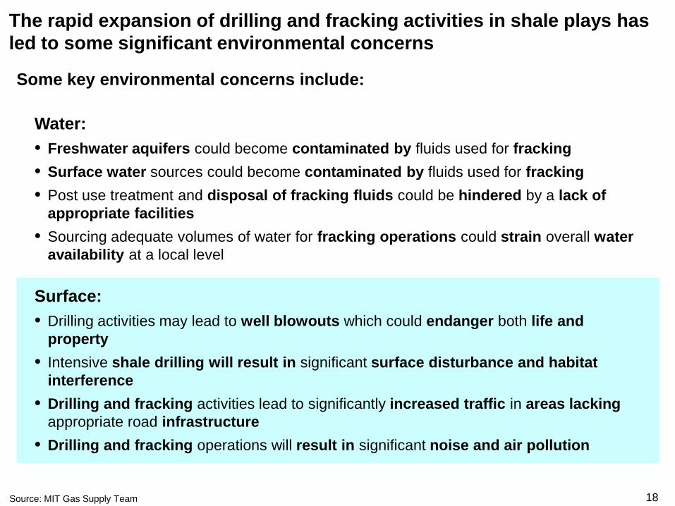
The rapid expansion of drilling and fracking activities in shale plays has led to some significant environmental concerns
Some key environmental concerns include:
Water:• Freshwater aquifers could become contaminated by fluids used for fracking• Surface water sources could become contaminated by fluids used for fracking• Post use treatment and disposal of fracking fluids could be hindered by a lack of
appropriate facilities• Sourcing adequate volumes of water for fracking operations could strain overall water
availability at a local level
Surface:• Drilling activities may lead to well blowouts which could endanger both life and
property • Intensive shale drilling will result in significant surface disturbance and habitat
interference• Drilling and fracking activities lead to significantly increased traffic in areas lacking
appropriate road infrastructure• Drilling and fracking operations will result in significant noise and air pollution

19
Shale gas production is facing a wide range of surface issues relating to water sourcing, transport and disposal
Illustration of shale well site and fluid containment pond
• Shale well drilling and completion can requires 5 million of more gallons of water
• Large volumes of injected frac water return to the surface – 20-70% flowbackdepending on situation
• Flowback water can be heavily polluted and needs to be treated
• Recovered water needs to be completely contained on site and properly disposed of to avoid pollution
• Permitted water treatment facilities not capable of handling frac fluid and drilling waste
• Underground injection capacity not adequate in some plays – PA in particular
• High transportation costs to haul frac water to treatment facilities
Some Challenges:
• On-site water treatment facilities and closed loop water reuse systems are being developed
• More efficient frac procedures are being deployed to reduce fluid injection volumes
• Operators are making more use of centralized production operations (pad well development) to reduce the need for water hauling
There is a strong economic incentive for operators to find solutions:
Source: MIT Gas Supply Team

The growth in shale gas production and the size of frac jobs has meant that annual shale gas related water demand is now at 20 billion gallons per year
20
0
500
1000
1500
2000
2500
3000
3500
4000
4500
5000
2005 2006 2007 2008 2009 2010
Marcellus
Woodford
Haynesville
Fayetteville
Barnett
Annual well additions in each of the major U.S. shale plays from 2005 – 2010 # of wells
0
2000
4000
6000
8000
10000
12000
14000
16000
18000
20000
2005 2006 2007 2008 2009 2010
Marcellus
Woodford
Haynesville
Fayetteville
Barnett
Annual water requirements for drilling and frackingin the major U.S. shale plays from 2005 – 2010 Millions of gallons of water
Source: MIT Gas Supply Team, HPDI commercial production database

However, it appears that water consumption for shale gas activities still represents a small portion of the total water usage in the major shale plays
21
0%
10%
20%
30%
40%
50%
60%
70%
80%
90%
100%
Barnett Fayetteville Haynesville Marcellus
Shale gas
Livestock
Irrigation
Industrial/Mining
Public supply
* “Modern Shale Gas: A Primer,” United States Department of Energy, April 2009Source: MIT Gas Supply Team
466 1,340 88 3,570
2008 water use by type in the major shale gas plays* Percent of total, Billions of gallons per year

22
Comments & Questions?

23
Supplemental materials

24
Along with intra-play variation, there is huge inter-play variation among the big shale plays – The Haynesville is very different to the Barnett
0
2,000
4,000
6,000
8,000
10,000
0 24 48 72 96 120
Difference between a typical Haynesville and Branett decline curve over the first 10 yearsMcf/day
• Haynesville wells have 30-day average IP of ~10,000 Mcf/day, compared to ~1,800 in the Barnett
• Haynesville wells experience 80-85% first year decline
• Haynesville wells produce up to 25% of EUR in year 1
0
1
2
3
4
5
6
2010 2020 2030 2040 2050 2060
0
2
4
6
8
10
12
2010 2020 2030 2040 2050 2060
10 Bcf/day5 Bcf/day
Decline in output upon cessation of drilling in the Haynesville shaleBcf/day
Decline onset sensitivity to output in Haynesville assuming EUR of 112 TcfBcf/day
Source: MIT Gas Supply Team analysis, HPDI commercial production database
Haynesville output is very sensitive to drilling activity

25
Cumulative probability of peak production rates of Fayetteville wells drilled in 2009Mcf/day (30-day average)
0 1,000 2,000 3,000 4,000 5,000 6,000
1
0.8
0.6
0.4
0.2
Cum
ulat
ive
Pro
babi
lity
P80
P50
P20
Source: MIT Gas Supply analysis HPDI production database
0 2,000 4,000 6,000 8,000 10,000 12,000
1
0.8
0.6
0.4
0.2
Cumulative probability of peak production rates of Woodford wells drilled in 2009Mcf/day (30-day average)
Cum
ulat
ive
Pro
babi
lity
P80
P50
P20
P20 P50 P80
Overall
Core
$3.74 $5.37 $8.77
$3.41 $4.65 $6.47
Variation in breakeven gas price for the ‘09 Fayetteville shale well population $/MMBtu
P20 P50 P80
Overall
Core
$4.71 $8.04 $20.12
$3.18 $3.73 $6.60
Variation in breakeven gas price for the ‘09 Woodford shale well population $/MMBtu
OverallCore
OverallCore
The analysis of well performance across shale plays is illustrating the variation in per-well economics that exists between and within the plays

26
Concern exists about direct contamination of fresh water aquifers due to fluid migration from a frac zone – analysis would suggest this is unlikely once wells were correctly completed
1000’s ft to shale layer
100’s ft to bottom of aquifer
BasinDepth to aquifer (ft)
Depth to shale (ft)
Barnett
Fayetteville
Marcellus
Woodford
Haynesville
6,500 –8,500
1,200
1450 –6,700
500
4,000 –8,500
850
6,000 –11,000
400
10,500 –13,500
400
Illustration of the scale of separation between freshwater aquifers and shale deposits
Depths to freshwater aquifers and producing layers in major shale plays*
Shale gas resources are separated from freshwater aquifers by 1,000s of feet of alternating layers of siltstones, shales, sandstones
* “Modern Shale Gas: A Primer,” United States Department of Energy, April 2009Source: MIT Gas Supply Team

27
There is a strong operational incentive to eliminate any fluid leakage since containment of the fluids in the shale is critical to the success of the “frac job”
* Michie & Associates. 1988. Oil and Gas Water Injection Well Corrosion. Prepared for the American Petroleum Institute.1988Source: MIT gas supply team
Illustration of multiple well casing used to isolate produced fluids from the aquifer in a gas well
Extensive regulation exists at State level regarding the protection of groundwater during oil and gas operations
• Current well design requirements demand extensive hydraulic isolation
• At depths coincident with the aquifer, groundwater will be separated from produced gas and fluids by at lease three layers of steel and three layers of cement
• The integrity of the isolation measures is tested
Probabilistic analysis for injection wells suggests the likelihood of a well leaking given properly installed casing is less than 1 in 1 million*
• Injection wells are consistently operated at high pressure, while production well pressure declines, further reducing the probability of leakage

28
Although frac fluids are almost entirely comprised of water and sand, a range of other chemicals are also present
Illustration of the composition of a typical fracing fluid*% by volume
99.51%Water & Sand
0.49%Chemical Additives
KCl
Gelling Agent
Scale Inhibitor
PH Adjustment
Breaker
Crosslinker
Iron Control
Acid
Friction Reducer
Corrosion Inhibitor
0.6%
0.1%
0.5%
0.3%
0.2%
0
0.4%
• Frac fluid composition varies from play to play due to the underlying geology; however, the vast majority of fluids are >98% sand and water
• Legitimate concerns have been raised about what additives are used in frac fluids, which the operators need to address in a more transparent manner
Biocide
* “Modern Shale Gas: A Primer,” United States Department of Energy, April 2009Source: MIT gas supply team