Embed Size (px)
Citation preview

arX
iv:1
607.
0558
3v2
[ph
ysic
s.ge
n-ph
] 1
1 O
ct 2
017
A New f(R) Model in the Light of Local Gravity Test and Late-time
Cosmology
Akhilesh Nautiyal∗a,b, Sukanta Panda†b, and Avani Patel‡b
aDepartment of Physics, Malaviya National Institute of Technology Jaipur, Jaipur 302 017,India
bDepartment of Physics, Indian Institute of Science Education and Research Bhopal, Bhopal462 066, India
Abstract
We propose a new model of f(R) gravity containing Arctan function in the lagrangian. Weshow here that this model satisfies fifth force constraint unlike a similar model in Kruglov 2013.In addition to this, we carry out the fixed point analysis as well as comment on the existence ofcurvature singularity in this model. The cosmological evolution for this f(R) gravity model is alsoanalyzed in the Freidmann Robertson Walker(FRW) background. To understand observationalsignificance of the model, cosmological parameters are obtained numerically and compared withthose of Lambda cold dark matter (ΛCDM) model. We also scrutinize the model with supernovadata. We apply Om diagnostic given by Sahni et al. 2008 to the model. Using this diagnostic, wedetect the distinction between cosmic evolution caused by the f(R) model and ΛCDM. We findbest-fit parameter values of the model using Baryon Acoustic Oscillations data.
1 Introduction
Recent progress in the precise measurements of cosmic microwave background anisotropies and ob-servations of type Ia supernovae and large scale structure strongly indicate that our universe, atpresent, is expanding acceleratingly [1]. An extra unknown component called dark energy is requiredto dominate over all other matter in recent times to make General Relativity (GR) enable to explainsuch accelerating expansion. These observations also suggest that the equation of state parameterof the unknown source should be negative. The simplest model which accommodates these featuresand is consistent with most of the observations is ΛCDM model, where Λ cosmological constant.The required value of the cosmological constant to fit with observations is many orders of magnitudesmaller than the value encountered from standard field theoretical calculations of vacuum energy [2].This large discrepancy forces us to look for alternative explanations for dark energy. One of suchalternatives is to replace the Ricci scalar, R, in Einstein-Hilbert action, by f(R), a general function ofR, which is known as f(R) theories of gravity [3,4]. If f(R) theory can mimick ΛCDM at high redshiftwithout using cosmological constant explicitly then the above discripancy can be circumvented. Thef(R) model studied here gives rise to effective cosmological constant in a sufficiently curved spacetime.This behaviour is a purely curvature induced effect and not related to vacuum energy.
Since observations favor cosmological constant as a best fit dark energy candidate, natural possi-bility for f(R) model is to construct one that can mimic as an effective cosmological constant todayand at the same time it should be distinguishable from ΛCDM model at recent times. With this clue,
∗[email protected]†[email protected]‡[email protected]
1

many f(R) models were proposed [5–16] which reduces to the ΛCDM model in large curvature limiti.e. f(R) → R− 2Λ for R >> Λ and tends to zero as R→ 0. The dynamical system analysis of f(R)theories are done in Ref. [17] wherein these theories are classified according to their fixed points. Anew approach for dynamical system analysis of f(R) models is established in [18] and applied to fewviable models in [18,19]. Any modified gravity theory should be put to the test to inquire that it doesnot spoil the successes of GR at local scales like the solar system. In general, all f(R) theories areeffective scalar-tensor theories with a potential term. If the mass of the scalar field is order of presentHubble parameter then it is difficult to satisfy the local gravity constraints due to the long-rangefifth force with a large coupling strength [20–22]. There must exist some screening mechanism whichscreens the fifth force in high-density region.
Many f(R) models are also plagued by fatal curvature singularities of various types. The cos-mological evolution happens at the minimum of the scalar field potential around which scalar fieldoscillates. The point of diverging curvature exists near the minimum at a finite potential in manyf(R) models [23–26]. The finite-time singularity in modified gravity is described in [27–32]. It isalso realized that the curvature singularities can be eliminated by adding an R2 term to the La-grangian [8, 24]. The curvature singularity can also be seen in an astrophysical object [23,26,33–35].The extensive investigations of singularities in relativistic stars are done in [36–38].
Though many modified gravity theories are becoming quite successful in explaining late-timeacceleration, they suffer from the problem that their physical implications cannot be distinguishedfrom each other. Many modified gravity models are also indistinguishable from ΛCDM. To solvethis, we need an observation based, a model-independent test which can distinguish above modelsphysically. A two-point diagnostic namely Om diagnostic to distinguish evolving dark energy modelsand ΛCDM model is given in [39]. The Om diagnostic is originally proposed in [40] as a null testof Dark Energy being a cosmological constant Λ. The brief discription of Om diagnostic is givenin Sec. 7. This two-point diagnostic is slightly modified in [41] by multiplying by h2 which wecall Omh2 diagnostic. An important property of the Omh2 diagnostic is that it uses expansionhistory H(z), whose value can be reconstructed from observations of luminosity distance DL viaa single differentiation. This Omh2 diagnostic can also provide a way to check the viabilities ofmodified gravity models and to distinguish them from each other as well as from ΛCDM. It is appliedto Starobinsky model [5] and Hu-Sawicki [6] model of f(R) gravity in [42]. In recent paper [43],observational constraints on f(R) models are obtained from cosmological chronometer, supernovaand baryon acoustic oscillations data.
In [23], a detailed study of local gravity tests and fixed-point analysis is done for an Arctan modelproposed in [16]. It turns out that this simple Arctan model is ruled out by fifth-force constraint.In this work, we propose a new Arctan model of f(R) gravity extending the model in [16]. Wecheck the viability of the model through local gravity test. In addition to this, we also carry outdynamical system analysis and find the fixed points for this model, following the line of [17]. Throughthe fixed point analysis, we show that our model and Hu-Sawicki model [6] belong to two differentclass of models. Cosmological evolution using this model is also presented by solving FRW equationsnumerically as described in [44]. The distance modulus calculated in this model is fitted with thesupernova data given by [45] for certain parameters. We investigate distinguishability of new f(R)model from ΛCDM model using Omh2(zi, zj) diagnostic. We also find the best parameter values forthe model by carrying out the χ2 test of Omh2 using Baryon Acoustic Oscillations data.
This paper progresses as follows. In the next section, we give a general idea of the modified Arctanmodel. The de Sitter points are obtained in Sec. 2.1 and Sec. 2.2 discusses the fixed points of themodel and their stability. The fifth-force test and its result are explained in Sec. 3. The investigationof curvature singularity is carried out in Sec. 4. Sec. 5 presents cosmological evolution and behaviorof density parameters and equation of state with the given modified Arctan model. The luminositydistance and distance modulus in this model along with the Union 2 compilation of supernova data isgiven in Sec. 6. The Omh2 Diagnostic of the f(R) model is carried out in Sec. 7. Finally, conclusionsare discussed in Sec. 8.
2

1
1.2
1.4
1.6
1.8
2
2.2
2.4
0 5 10 15 20 25 30 35 40 45 50 55
-βF(
R)
βR
arctann=1.75,b=1.021n=2.5,b=1.021n=1.75,b=1.3
Figure 1: −βF (R) Vs. βR. In ”arctan” curve n = 1 and b = 1.021 are taken.
2 A New f(R) Model
In f(R) theory, Hilbert-Einstein action is replaced by a more general action
S =
∫
d4x√−g
[
1
2κ2f(R) + Lm
]
, (1)
where f(R) is an arbitrary function of Ricci scalar R and Lm is usual matter Lagrangian. It is moreconvenient to write the function f(R) as f(R) = R + F (R), where F (R) is an arbitrary functionof R. It can be easily seen that one can retain GR and ΛCDM for F (R) = 0 and F (R) = −2Λrespectively. Another benefit of writing f(R) in this way is that effects of modification to Einsteingravity is more evident and its study becomes simpler. Here, we propose a new model of f(R) theory,slightly modifying Arctan model given in [16],
F (R) = − b
βArctan(βR)n. (2)
Here, b, β and n are positive constants. β has the inverse dimension of Ricci scalar R and it is of theorder of inverse of presently observed effective cosmological constant. Note that our model reducesto the Arctan model proposed in [16] for n = 1. Whenever we write ”Arctan model” throughoutthis paper we mean the model in [16]. In Fig. 1, the function −βF (R) is plotted w.r.t. βR fordifferent values of n. One can see from the Fig. 1 that the variations in βF (R) occurs only betweenβR ∼ 1−5. Beyond βR ∼ 5, the value of βF (R) becomes nearly constant. This behaviour tells us thatour model given in Eq. (2) mimics as ΛCDM at high curvature i.e. at R >> 1/β and f(R) becomeszero at R = 0. Also, notice that the function F (R) increases and becomes constant more rapidly asn increases, which suggests that the value of parameter n should be small enough so that the modelcan explain correct cosmic history. While keeping n constant, the shape of the curve remains same,but its magnitude increases with increasing b.
2.1 Constant Curvature Solution
By varying the action written in Eq. (1) w.r.t. gµν we obtain the field equation given as,
f,RRab −1
2fgab − (∇a∇b − gab) f,R = κ2Tab. (3)
Here κ2 = 8πG and is the covariant D’Alambertian. Any quantity with , R in the subscript denotesderivative w.r.t R. Eq. (3) can also be written in the following form by using the expression for
3

Einstein tensor Gab
f,RGab − f,RR∇a∇bR− f,RRR (∇aR) (∇bR) + gab
[
1
2(Rf,R − f) + f,RRR+
f,RRR (∇R)2]
= κ2Tab, (4)
where (∇R)2 = gab (∇aR) (∇bR). The trace of the above field equation is given by
3f,RR(R)R− 2f(R) +Rf,R + 3f,RRR (∇R)2 = κ2T (5)
which can be rewritten as
R =1
3f,RR
[
κ2T − 3f,RRR (∇R)2 + 2f −Rf,R
]
(6)
The constant curvature solution of Eq. (6) in vacuum describes the de Sitter universe. It correspondsto the condition
2f(Rd)−Rdf,R(Rd) = 0, (7)
having de Sitter point denoted as Rd. A few de Sitter points for different values of n and b are listedin Table 1. A de Sitter point Rd is a stable point describing primordial and present vacuum energydominated epoch if it satisfies the condition F,R(Rd)/F,RR(Rd) > Rd. All the de Sitter points givenin Table 1 are stable de Sitter points. The quantity f,R is identified with scalar field φ in f(R) theory.We will discuss more about it in Sec. 4. The conditions for graviton to be of non-ghost nature andscalar field φ to be non techyonic are f,R > 0 and f,RR > 0 respectively. They are investigated forthe model in Eq. (2) and it is found that both the conditions are satisfied by all parameter valuesmentioned in Table 1 for Rd < R < ∞. In the following sections, we will find that parameter valueswith n ≥ 1.75 and b ≥ 1.021 are constrained by local gravity tests and n = 1.75 and b = 3.0 is thebest choice according to Omh2 diagnostic.Using Eq. (6) and (7) we can define a potential
V (R) = −Rf(R)3
+
∫ R
f(R⋆)dR⋆, (8)
such that dV (R)dR
=2f(R)−Rf,R
3 = 0 for the minimum at the de Sitter point. The potential for some ofthe choices of parameters shown in Table 1 is shown in Fig. 2.
n b βRd1.75 1.021 2.40921.75 1.1 2.77771.75 1.5 4.27081.75 2.0 5.95301.75 3.0 9.19301.0 2.0 5.13970.98 5.0 14.6369
Table 1: de Sitter points for different values of b and n
2.2 Fixed Point Analysis
It is necessary to carry out fixed point analysis in order to check whether given model can give rise todark energy dominated era preceded by matter dominated era or not. In this section, we find the fixedpoints for the model (2) and also for Hu-Sawicki model proposed in [6]. Through this analysis, we show
4

Figure 2: V (R)/H40 vs βR for the model (2) and the potential V (R) is defined by Eq. (8)
that our model belongs to different class than the Hu-Sawicki model does and therefore both modelsare phenomenologically distinguishable from each other. Here, we follow the procedure followed bymany authors and originally proposed in [17]. Assuming background spacetime as a spatially flat FRWspacetime, field equations can be written as evolution equations in terms of R, R, Hubble constantH and matter density ρm. These evolution equations can be further written as a set of dynamicalsystem equations by defining dimensionless variables y1 ≡ − ˙f,R/Hf,R, y2 ≡ −f/6f,RH2, y3 ≡ R/6H2
and y4 ≡ κ2ρr/3f,RH2 together with the density parameters Ωm ≡ 1 − y1 − y2 − y3 − y4, Ωr ≡ y4
and ΩDE ≡ y1 + y2 + y3. Solving the set of dynamical system equations, in the absence of radiation(y4 = 0), one can obtain several fixed points namely P1, P2, P3, P4, P5 and P6. As described in [17],among these fixed points, either P1 or P6 can give rise to late-time aceleration. The point P1 is deSitter point for which condition (7) is satisfied. Basically, this dynamical system can be characterizedby two quantities
m ≡ Rf,RRf,R
, (9)
r ≡ −Rf,Rf
=y3y2. (10)
The m and r for our model given in (2) can be written in terms of x = βR as follows
m =2bn2x3n−1 − bn(n− 1)xn−1(1 + x2n)
(1 + x2n)(1 + x2n − bnxn−1), (11)
r =−x− x2n+1 + bnxn
(1 + x2n)(x− bArcTan(xn)). (12)
The function f(R) for Hu-Sawicki model [6] and m and r are given by
f(R) = R− c1β(βR)n (1 + c2(βR)
n)−1 (13)
m =(1 + c2x
n)−3(
−(2n − 1)nc1c2x2n−1 + nc1c2x
3n−1)
1− nc1c2x2n−1(1 + c2xn)−2, (14)
r = −−x− nc1c2x2n(1 + c2x
n)−2
x− c1xn(1 + c2xn)−1. (15)
In Figures 3 and 4, m(r) curve is plotted on (r,m) plane for the function given in Eq. (2) and Eq.(13) respectively. The points P5 and P6 exist on m = −r − 1 line. The saddle matter era is realizedby fixed point P5. The condition for the existence of saddle point P5 is m(r) = +0, dm/dr > −1,
5

P6
P1
P5
- 3.0 - 2.5 - 2.0 -1.5 -1.0 - 0.50.0
0.5
1.0
1.5
2.0
r
m
m Vs . r for b =1.021 and n =1.75
Figure 3: m Vs. r. Red and yellow lines are m = −r − 1 and r = −2 line respectively.
-0.4
-0.3
-0.2
-0.1
0
0.1
0.2
0.3
0.4
0.5
0.6
0.7
-1.6 -1.5 -1.4 -1.3 -1.2 -1.1 -1
m(r
)
r
P6
P5
m(r)-r-1
Figure 4: m Vs. r for Hu-Sawicki model for n = 4. c1 and c2 are fixed using condition |F,R0= 0.01|.
Green line is m = −r − 1 line.
at r = −1. If we take limit βR → ∞ in expressions of r in Eq. (12) and Eq. (15), we can obtainr → −1. Calculating dm/dr from (dm/dR)/(dr/dR) and taking R → ∞ limit in it, one can end upwith dm/dr(r = −1) ≥ −1. This says that P5 is a saddle point showing existence of saddle matterera in our model and also in Hu-Sawicki model at very large curvature. The stability condition forthe point P6 is m = −r − 1, (
√3 − 1)/2 < m < 1 which is satisfied in Hu-Sawicki model but not in
our model as evident from the Figures 3 and 4. Lastly, the de Sitter point P1 for the model (2), aswe have already obtained in Sec. 2.1, is a stable point. This can be also proved from its stabilitycondition (r = −2, 0 < m ≤ 1) which is clearly satisfied by our model. Therefore, we can concludethat the model given in Eq. (2) gives the evolution of our universe from saddle matter era (pointP5) to a de Sitter state (point P1) through blue curve shown in Fig. 3 while m = 0 line shows theΛCDM evolution. The universe given by Hu-Sawicki model evolves from saddle matter era (pointP5) to a late-time accelerating phase (point P6) through red curve shown in Fig. 4. In the language
6

of [17], any satisfacory f(R) model belongs to either class II: the matter epoch is followed by a deSitter acceleration (connecting P5 to P1) or class IV: the matter epoch is followed by a nonphantomaccelerated attractor (connecting P5 to P6). From this analysis, we can say that our model given in(2) belongs to class II and Hu-Sawicki model given in (13) belongs to class IV.
3 Fifth Force Constraint
It is well-known that the f(R) theory has an extra scalar degree of freedom in addition to usualgraviton. Since the scalar field is a dynamical degree of freedom, it gives rise to a propagating fifth-force which is the cause of the late-time acceleration. But, it must be suppressed at the local gravityscales in order to evade experimental results of solar system tests and EP(Equivalence Principle)violation tests. The condition for the suppression of fifth force on local gravity scales is given bym2φL
2s >> 1, where mφ is the mass of the scalar field and Ls is the typical length scale involved in
experiment [20,21]. One can calculate the value of m2φ for our model given in (2), which comes out to
be of the order of 10−51m−2. Considering Ls = 1m, the above condition can be seen to be completelyviolated.In the Einstein frame, the scalar field of an f(R) theory is a chameleon-like field which exhibitschameleon mechanism given by [46]. The name owes to the fact that the ”chameleon” field blendswith the environment in the highly dense background and becomes invisible to any experimentalsearches for fifth-force. This is because the mass of the field depends on the background density. Itcan be shown as following. The action in Eq. (1) can be written, via a conformal transformation, inEinstein frame as
S =
∫
d4x√
−g[
R
2κ2− (∇ψ)2
2− VE(ψ) + Lm(gµνe
−
2√
6κψ
)
]
. (16)
Here, all quantities having tilde are defined in Einstein frame. The Einstein frame scalar field ψ isrelated to function f(R) by the relation κψ =
√
3/2 ln f,R. Let us consider the spherically symmetricbody with radius rc. Varying action in (16) w.r.t. ψ we obtain the field equation for ψ as
d2ψ
dr2+
2
r
dψ
dr− dVeff
dψ= 0. (17)
The effective potential Veff is given by
Veff (ψ) = VE(ψ) + e− 2√
6κψρ∗. (18)
Because of the interplay of two terms self-interaction potential VE and conformal coupling to thematter, the effective potential possesses the global minimum. By solving the dynamical equation(17), one can find that the scalar field ψ is frozen at the potential minimum with a very smallmagnitude and its mass is very high. Thus, its contribution to the field outside is negligible exceptfor a thin shell regime near the surface of the object. The thin-shell condition is given by
δrcrc
= −ψout − ψin√6Φc
. (19)
Where, Φc is the gravitational potential on the surface of the test body (Sun/Earth) and δrc is thethickness of the thin shell. Here, ψout and ψin are value of the field at the minima of Veff outsideand inside the body respectively. If ψin << ψout the the thin-shell condition written in Eq.(19) canbe reduced to
|ψout| ≃√6Φc
δrcrc. (20)
The experimental results of the solar system tests and the EP violation [22,47] tests put the constraints
7

20 40 60 80 100
2
4
6
8
10
Β Rd
n
Ψout < 3.43 ´ 10- 15
Figure 5: Shaded region is the allowed region for different values of parameter n and βRd.
on the r.h.s. of the Eq. (20):
.
5.97 × 10⁻¹¹ (Solar system test),3.43 × 10−15 (EP test).
(21)
For the model given in (2), ψout can be written as
ψout ≈√6
2F,R|R=ρout
=
√6
2
[
(−nb)(βρout)n−1
1 + (βρout)2n
]
. (22)
Here, we have considered the approximation that R >> 1/β. Let us put βρout = βRdρoutRd
. Since
ρout ≃ 10−24g/cm3 and Rd ≃ ρc ∼ 10−29g/cm3 one can write βρout ≃ βRd × 105 in Eq. (22).
ψout ≈√6
2
[
−nb (βRd × 105)n−1
1 + (βRd × 105)2n
]
(23)
From the de Sitter condition in Eq. (7), parameter b can be written in terms of n and βRd as
b =−βRd
−2Arctan(βRd)n +n(βRd)n
1+(βRd)2n
. (24)
Plugging Eq. (24) into Eq. (23), one ends up with the expression
|ψout| ≈
∣
∣
∣
∣
∣
∣
−n√6
2
−βRd−2Arctan(βRd)n +
n(βRd)n
1+(βRd)2n
× (βRd × 105)n−1
1 + (βRd × 105)2n
∣
∣
∣
∣
∣
∣
(25)
With the help of Eq. (25) and Eq. (21) we can put the constraint on our model parameters to evadethe fifth-force constraint. Fig. 5 exhibits allowed regions for different values of parameter n and βRd.From the Fig. 5, one can conclude that b ≥ 1.021 and n ≥ 1.75 to evade the local gravity test. Thecorresponding de Sitter point βRd has to be ≥ 2.4.
8
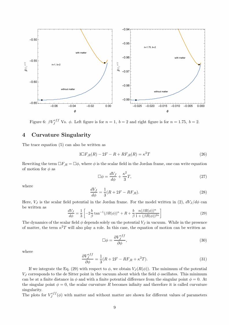
Figure 6: βV effJ Vs. φ. Left figure is for n = 1, b = 2 and right figure is for n = 1.75, b = 2.
4 Curvature Singularity
The trace equation (5) can also be written as
3F,R(R)− 2F −R+RF,R(R) = κ2T (26)
Rewriting the term F,R = φ, where φ is the scalar field in the Jordan frame, one can write equationof motion for φ as
φ =dVJdφ
+κ2
3T, (27)
wheredVJdφ
=1
3(R + 2F −RF,R). (28)
Here, VJ is the scalar field potential in the Jordan frame. For the model written in (2), dVJ/dφ canbe written as
dVJdφ
=1
3
[
−2b
βtan−1(βR(φ))n +R+
b
β
n(βR(φ))n
1 + (βR(φ))2n
]
(29)
The dynamics of the scalar field φ depends solely on the potential VJ in vacuum. While in the presenceof matter, the term κ2T will also play a role. In this case, the equation of motion can be written as
φ =∂V eff
J
∂φ, (30)
where∂V eff
J
∂φ=
1
3(R+ 2F −RF,R + κ2T ). (31)
If we integrate the Eq. (29) with respect to φ, we obtain VJ(R(φ)). The minimum of the potentialVJ corresponds to the de Sitter point in the vacuum about which the field φ oscillates. This minimumcan be at a finite distance in φ and with a finite potential difference from the singular point φ = 0. Atthe singular point φ = 0, the scalar curvature R becomes infinity and therefore it is called curvaturesingularity.The plots for V eff
J (φ) with matter and without matter are shown for different values of parameters
9

n and b in Fig. 6. The black dots are minima of the potential V effJ . It can be easily seen that the
minimum moves closer to the singularity in the presence of matter thus making the scalar field morevulnerable to meet the singularity. The minimum is at a closer distance for larger values of n asevident from the Fig. 6. Therefore the Arctan model is safer than our model in (2) but not free fromfatal curvature singularity at all. But, the curvature singularity can be cured by adding R2 term tothe Lagrangian since it can increase the potential VJ to the infinity as φ approaches the singularityfor fine-tuned parameter values as suggested in [8].
5 Cosmological Evolution
In this section, we discuss cosmological implications of the model given in Eq. (2). We considerhomogeneous and isotropic FRW universe described by the metric
ds2 = −dt2 + a2(t)
[
dr2
1−Kr2+ r2
(
dθ2 + sin2 θdφ2)
]
(32)
Using Eq. (6) with above spacetime we get
R = −3HR− 1
3f,RR
[
3f,RRRR2 + 2f − f,RR + κ2T
]
(33)
The cosmological evolution can be obtained by solving field equation (4) with FRW metric anddiagonal energy-momentum tensor. The equations governing the scale factor and Hubble constant Hfor flat FRW universe are given as
H2 +1
f,R
[
f,RRHR− 1
6(f,RR− f)
]
= −κ2T tt3f,R
, (34)
H = −H2 +1
f,R
(
f,RRHR+f
6+κ2T tt3
)
, (35)
where H = aa. The expression for the Ricci scalar in terms of Hubble constant directly obtained from
the metric is given by
R = 6
(
H + 2H2 +K
a2
)
(36)
The energy-momentum tensor considered for cosmological evolution has three contributions i.e.baryon, radiation, and dark matter. The conservation equation ∇aT
ab = 0, satisfied by each compo-nent separately, leads to the following equation,
ρT + 3H (ρT + pT ) = 0. (37)
Here the total energy density is ρT = ρbar + ρDM + ρrad. The above equation can be integrated byusing pbar, pDM = 0 and prad = ρrad/3 and the energy density can be expressed in terms of scalefactor as
ρT =ρ0bar + ρ0DM(a/a0)
3 +ρ0rad
(a/a0)4 , (38)
where the knotted quantities indicate their values today. The time-time component of the energy-momentum tensor and its trace appearing in equations (33), (34) and (35) can be written in terms ofenergy density and pressure as T tt = −ρT and T = − (ρbar + ρDM ).
Now to obtain the equation of state of f(R) gravity one can define the energy density ρX suchthat the Friedmann equation (34) looks like
H2 =κ2
3(ρ+ ρX) . (39)
10

0
20
40
60
80
100
120
140
160
180
200
220
-1 0 1 2 3 4 5
R
z
n = 1.75, b = 1.021, βRd = 2.4032
6.13
6.135
6.14
6.145
6.15
6.155
-1 -0.98 -0.96 -0.94 -0.92 -0.9 -0.88 -0.86
0
1
2
3
4
5
6
7
8
9
-1 0 1 2 3 4 5
H
z
n = 1.75, b = 1.021, βRd = 2.4032ΛCDM
0.715
0.7155
0.716
0.7165
0.717
0.7175
0.718
-1 -0.98 -0.96 -0.94 -0.92 -0.9 -0.88 -0.86
Figure 7: Left figure is R Vs. z and right figure is H Vs. Z
0
50
100
150
200
250
300
350
400
450
500
-1 0 1 2 3 4 5 6 7
R
z
n = 1.75, b = 1.5, βRd = 4.2708
7.645 7.6455 7.646
7.6465 7.647
7.6475 7.648
7.6485 7.649
7.6495
-1 -0.98 -0.96 -0.94 -0.92 -0.9 -0.88 -0.86
0
2
4
6
8
10
12
14
-1 0 1 2 3 4 5 6 7
H
z
n = 1.75, b = 1.5, βRd = 4.2708
0.7982
0.7983
0.7984
0.7985
0.7986
0.7987
0.7988
-1 -0.98 -0.96 -0.94 -0.92 -0.9 -0.88 -0.86
Figure 8: Left figure is R Vs. z and right figure is H Vs. Z
0
50
100
150
200
250
300
350
400
450
500
-1 0 1 2 3 4 5 6 7
R
z
n = 1.75, b = 2.0, βRd = 5.9530
8.0355
8.036
8.0365
8.037
8.0375
8.038
8.0385
-1 -0.98 -0.96 -0.94 -0.92 -0.9 -0.88 -0.86
0
2
4
6
8
10
12
14
-1 0 1 2 3 4 5 6 7
H
z
n = 1.75, b = 2.0, βRd = 5.9530
0.8183
0.8184
0.8185
0.8186
0.8187
0.8188
0.8189
0.819
-1 -0.98 -0.96 -0.94 -0.92 -0.9 -0.88 -0.86
Figure 9: Left figure is R Vs. z and right figure is H Vs. Z
11

0
50
100
150
200
250
300
350
400
450
500
-1 0 1 2 3 4 5 6 7
R
z
n = 1.75, b = 3.0, βRd = 9.1931
8.248 8.2485 8.249
8.2495 8.25
8.2505 8.251
8.2515
-1 -0.98 -0.96 -0.94 -0.92 -0.9 -0.88 -0.86
0
2
4
6
8
10
12
14
-1 0 1 2 3 4 5 6 7H
z
n = 1.75, b = 3.0, βRd = 9.1931
0.829
0.8291
0.8292
0.8293
0.8294
0.8295
0.8296
-1 -0.98 -0.96 -0.94 -0.92 -0.9 -0.88 -0.86
Figure 10: Left figure is R Vs. z and right figure is H Vs. Z
0
1
2
3
4
5
6
7
8
9
-1 0 1 2 3 4 5
H
z
ΛCDM
0.8366 0.83665
0.8367 0.83675
0.8368 0.83685
0.8369 0.83695
0.837 0.83705
0.8371 0.83715
-1 -0.98 -0.96 -0.94 -0.92 -0.9 -0.88 -0.86
Figure 11: H Vs. z for ΛCDM.
12

Similarly the pressure pX can also be defined in a way so that the Eq. (35) will become
H +H2 = −κ2
6(ρ+ ρX + 3(prad + pX)) . (40)
Now using the above two equations along with Eq. (34) and Eq. (35) the energy density and pressurefor f(R) fluid can be written as
ρX =1
κ2f,R
[
1
2(f,RR− f)− 3f,RRHR+ κ2ρ (1− f,R)
]
, (41)
pX = − 1
3κ2f,R
[
(f,RR + f)
2+ 3f,RRHR− κ2 (ρ− 3pradf,R)
]
. (42)
With these expressions of energy density and pressure, we can write the equation of state for f(R) as
wX =pXρX
. (43)
The equation of state wX can also be written in the following form by using Eqns. (39), (40), and(36) as
wX =3H2 − 3κ2prad −R
3 (3H2 − κ2ρ). (44)
To obtain the behavior of R andH w.r.t redshift z, we solve Eqns.(33), (34), (35), and (36) numericallyusing the method described in [44]. To integrate these differential equations we choose
α = ln(a/a0) (45)
as an independent variable instead of t since α → −∞ as a → 0 is well kept far from the regime ofintegration. Also, it is easy to get the quantities R and H in terms of redshift z = e−α−1. Eqns. (33),(34), (35) and (36) can be expressed in terms of α as
R′′ = −R′
(
1 +R
6H2
)
− 1
3f,RRH2
[
3f,RRRH2R′2 + 2f − f,RR+ κ2T
]
, (46)
H ′ = −2H +R
6H, (47)
H2 +1
f,R
[
f,RRH2R′ − 1
6(f,RR− f)
]
= −κ2T tt3fR
, (48)
H ′ = −H +1
f,RH
(
f,RRH2R′ +
f
6+κ2T tt3
)
, (49)
where ’ denotes the derivative w.r.t. α.To numerically integrate the above differential equations we can use either Eq. (47) or (49) for H.
To check the consistency of the code we have used both. Eq. (48) is modified Hamiltonian constraintand can be used to determine the accuracy of the code. The initial conditions for R and H are takenas described in [44].
The behavior of Ricci scalar R and Hubble constant H is depicted in Figs. 7 to 10 for the choiceof the parameters given in Table 1. As ahown in the inset figures which is a zoomed, The Ricciscalar oscillates around its value at the de Sitter point today, which can be seen by applying linearperturbations (see Fig. 2) around the de Sitter minimum. The Hubble constant today also oscillates.From Fig. 10 we see that the oscillations are not significant for larger value of b with n = 1.75. InFig. 7, evolution of H(z) in ΛCDM is also shown for the comparision.
13

The dimensionless densities for different species can be expressed as
Ω := Ωrad +Ωbar +ΩDM +ΩX = 1, (50)
where Ωi =κρi3H2 . The density for the f(R) model is given by (41). The variation of matter density
ΩM and the density of f(R) model (2) ΩX w.r.t z is shown in Figs. 12 and 13 for the values of n andb given in Table 1. We have also plotted the same densities for the ΛCDM model for reference. Thevarious density parameters Ωi for the ΛCDM model can be expressed in terms of their values todayas
ΩΛCDMi =
Ω0ΛCDMi aI
[(
Ω0ΛCDMbar +Ω0 ΛCDM
DM
)
a−3 +Ω0 ΛCDMrad a−4 +Ω0
Λ
] . (51)
Here i represents baryon, dark matter, radiation and Λ and I = −3, −3, −4, 0 for these speciesrespectively. It is clear from the Figs. 12 and 13 that the variation of Ωi w.r.t z is not much differentfor all the choices of the parameters n and b. It is also clear from the Figs. 12 and 13 that thef(R) model (2) presented in this work exhibit sufficiently long matter dominated era as predicted byfixed point analysis presented in Sec. 2.2. For larger redshift ΩX behaves in a similar way as ΩΛ sowe expect a radiation era in the early universe similar to ΛCDM model so that the predictions ofNucleosynthesis are not spoiled.
0
0.2
0.4
0.6
0.8
1
-1 0 1 2 3 4 5 6 7
Ωi
z
ΩX ΩM
n = 1.75, b = 1.021, βRd = 2.4032n = 1.75, b =1.1, βRd = 2.7733n = 1.75, b = 1.5, βRd = 4.2708n = 1.75, b =2.0, βRd = 5.9530n = 1.75, b = 3.0, βRd = 9.1931n = 0.98, b =5.0, βRd = 14.6369
Figure 12: Ωi vs z
0
0.2
0.4
0.6
0.8
1
-1 0 1 2 3 4
Ωi
z
ΩX ΩM
n = 1.75, b = 1.021, βRd = 2.4032n = 1.75, b = 3.0, βRd = 9.1931n = 0.98, b =5.0, βRd = 14.6369
ΛCDMArcTan
Figure 13: Ωi vs z
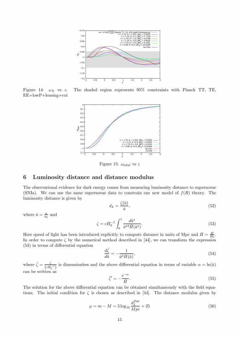
Figs. 14 and 15 show the behavior of equation of state of the f(R) component of the fluid given by(2) and the equation of state of the total fluid. In Fig. 14, one can note that the values of equation ofstate for parameters with values n = 1.75 and b = 2, 3 lie in the shaded region which shows the 95%constraints with Planck TT, TE, EE+lowP+lensing+ext. From Fig. [14] we see that the equationof state for the f(R) model (2) exhibits oscillation around phantom divide ω = −1 for all choice ofparameters. The existence of matter era for higher redshifts can also be seen from the behavior ofωtotal as depicted in Fig. 15.
14
−1.2
−1.15
−1.1
−1.05
−1
−0.95
−0.9
−0.85
−0.8
−0.75
−1 −0.5 0 0.5 1 1.5 2 2.5 3ω X
z
w=−1.019+0.075−0.080 Planck TT, TE, EE+lowP+lensing+ext
n = 1.75, b = 1.021, βRd = 2.4032n = 1.75, b =1.1, βRd = 2.7733
n = 1.75, b = 1.5, βRd = 4.2708n = 1.75, b =2.0, βRd = 5.9530
n = 1.75, b = 3.0, βRd = 9.1931n = 0.98, b =5.0, βRd = 14.6369
ArcTan
Figure 14: ωX vs z. The shaded region represents 95% constraints with Planck TT, TE,EE+lowP+lensing+ext
-1.1
-1
-0.9
-0.8
-0.7
-0.6
-0.5
-0.4
-0.3
-0.2
-0.1
0
-1 -0.5 0 0.5 1 1.5 2 2.5 3
ω tot
al
z
n = 1.75, b = 1.021, βRd = 2.4032n = 1.75, b =2.0, βRd = 5.9530n = 1.75, b = 3.0, βRd = 9.1931n = 0.98, b =5.0, βRd = 14.6369
ArcTanΛCDM
Figure 15: ωtotal vs z
6 Luminosity distance and distance modulus
The observational evidence for dark energy comes from measuring luminosity distance to supernovae(SNIa). We can use the same supernovae data to constrain our new model of f(R) theory. Theluminosity distance is given by
dL =ζ(a)
a, (52)
where a = aa0
and
ζ = cH−10
∫ 1
a
da⋆
a⋆2H(a⋆). (53)
Here speed of light has been introduced explicitly to compute distance in units of Mpc and H = HH0
.In order to compute ζ by the numerical method described in [44], we can transform the expression(53) in terms of differential equation
dζ
da= − 1
a2H(a), (54)
where ζ = ζ
(cH−1
0 )is dimensionless and the above differential equation in terms of variable α = ln(a)
can be written as
ζ ′ = −e−α
H. (55)
The solution for the above differential equation can be obtained simultaneously with the field equa-tions. The initial condition for ζ is chosen as described in [44]. The distance modulus given by
µ = m−M = 5 log10dflatL
Mpc+ 25 (56)
15

is the quantity reported by supernovae data. Figs. 16 and 17 show variation of luminosity distance and
0
5000
10000
15000
20000
25000
30000
35000
40000
45000
50000
0 1 2 3 4 5
d L (M
pc)
z
n = 1.75, b = 1.021, βRd = 2.4032n = 1.75, b =2.0, βRd = 5.9530n = 1.75, b = 3.0, βRd = 9.1931n = 0.98, b =5.0, βRd = 14.6369
ArcTanΛCDM
Figure 16: Luminosity distance vs z
32
34
36
38
40
42
44
46
-2 -1.5 -1 -0.5 0
m-M
log z
n = 1.75, b = 1.021, βRd = 2.4032n = 1.75, b =2.0, βRd = 5.9530n = 1.75, b = 3.0, βRd = 9.1931n = 0.98, b =5.0, βRd = 14.6369
ArcTanΛCDM
Figure 17: Distance modulus vs z
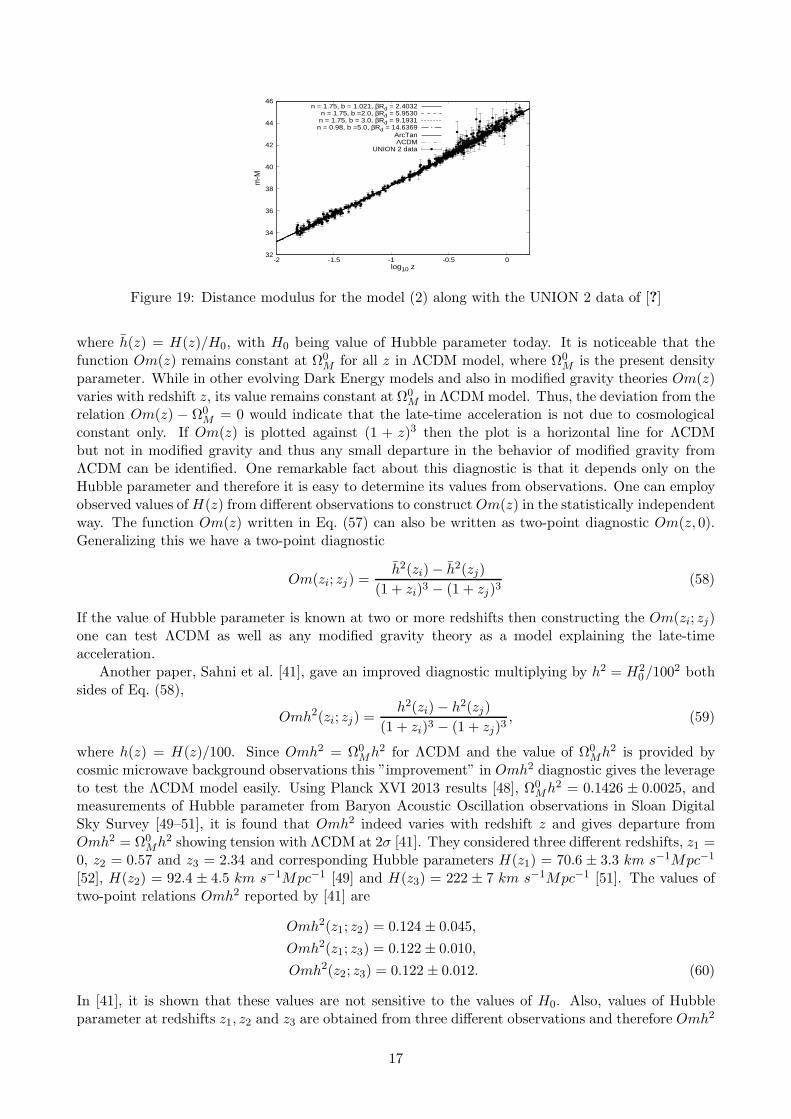
distance modulus w.r.t z for the f(R) model (2) along with the ΛCDM. The luminosity distance anddistance modulus for the model are not much different from the ΛCDM for all choice of parameters.Distance modulus is also plotted along with the supernovae data of UNION 2 [45] in Figs. 18 and 19.In the next section, we apply Omh2 diagnostic to test f(R) model written in Eq. (2).
26
28
30
32
34
36
38
40
42
44
46
0 0.5 1 1.5 2
m-M
z
n = 1.75, b = 1.021, βRd = 2.4032n = 1.75, b =2.0, βRd = 5.9530n = 1.75, b = 3.0, βRd = 9.1931n = 0.98, b =5.0, βRd = 14.6369
ArcTanΛCDM
UNION 2 data
Figure 18: Distance modulus for the model (2) along with the UNION 2 data of [?]
7 Omh2 Diagnostic
Starting with the Hubble parameter, Sahni et al. [40] proposed a new diagnostic namely Om diag-nostic:
Om(z) =h2(z)− 1
(1 + z)3 − 1, (57)
16
32
34
36
38
40
42
44
46
-2 -1.5 -1 -0.5 0m
-Mlog10 z
n = 1.75, b = 1.021, βRd = 2.4032n = 1.75, b =2.0, βRd = 5.9530n = 1.75, b = 3.0, βRd = 9.1931n = 0.98, b =5.0, βRd = 14.6369
ArcTanΛCDM
UNION 2 data
Figure 19: Distance modulus for the model (2) along with the UNION 2 data of [?]
where h(z) = H(z)/H0, with H0 being value of Hubble parameter today. It is noticeable that thefunction Om(z) remains constant at Ω0
M for all z in ΛCDM model, where Ω0M is the present density
parameter. While in other evolving Dark Energy models and also in modified gravity theories Om(z)varies with redshift z, its value remains constant at Ω0
M in ΛCDM model. Thus, the deviation from therelation Om(z) − Ω0
M = 0 would indicate that the late-time acceleration is not due to cosmologicalconstant only. If Om(z) is plotted against (1 + z)3 then the plot is a horizontal line for ΛCDMbut not in modified gravity and thus any small departure in the behavior of modified gravity fromΛCDM can be identified. One remarkable fact about this diagnostic is that it depends only on theHubble parameter and therefore it is easy to determine its values from observations. One can employobserved values ofH(z) from different observations to construct Om(z) in the statistically independentway. The function Om(z) written in Eq. (57) can also be written as two-point diagnostic Om(z, 0).Generalizing this we have a two-point diagnostic
Om(zi; zj) =h2(zi)− h2(zj)
(1 + zi)3 − (1 + zj)3(58)
If the value of Hubble parameter is known at two or more redshifts then constructing the Om(zi; zj)one can test ΛCDM as well as any modified gravity theory as a model explaining the late-timeacceleration.
Another paper, Sahni et al. [41], gave an improved diagnostic multiplying by h2 = H20/100
2 bothsides of Eq. (58),
Omh2(zi; zj) =h2(zi)− h2(zj)
(1 + zi)3 − (1 + zj)3, (59)
where h(z) = H(z)/100. Since Omh2 = Ω0Mh
2 for ΛCDM and the value of Ω0Mh
2 is provided bycosmic microwave background observations this ”improvement” in Omh2 diagnostic gives the leverageto test the ΛCDM model easily. Using Planck XVI 2013 results [48], Ω0
Mh2 = 0.1426 ± 0.0025, and
measurements of Hubble parameter from Baryon Acoustic Oscillation observations in Sloan DigitalSky Survey [49–51], it is found that Omh2 indeed varies with redshift z and gives departure fromOmh2 = Ω0
Mh2 showing tension with ΛCDM at 2σ [41]. They considered three different redshifts, z1 =
0, z2 = 0.57 and z3 = 2.34 and corresponding Hubble parameters H(z1) = 70.6 ± 3.3 km s−1Mpc−1
[52], H(z2) = 92.4 ± 4.5 km s−1Mpc−1 [49] and H(z3) = 222 ± 7 km s−1Mpc−1 [51]. The values oftwo-point relations Omh2 reported by [41] are
Omh2(z1; z2) = 0.124 ± 0.045,
Omh2(z1; z3) = 0.122 ± 0.010,
Omh2(z2; z3) = 0.122 ± 0.012. (60)
In [41], it is shown that these values are not sensitive to the values of H0. Also, values of Hubbleparameter at redshifts z1, z2 and z3 are obtained from three different observations and therefore Omh2
17

0.24
0.26
0.28
0.3
0.32
0.34
0.36
0.38
0.4
0 0.5 1 1.5 2 2.5 3
Om
(z)
z
ΩM0=0.26
ΩM0=0.28
ΩM0=0.30
ΩM0=0.32
0.24
0.26
0.28
0.3
0.32
0.34
0.36
0.38
0.4
0 0.5 1 1.5 2 2.5 3
Om
(z)
z
ΩM0=0.26
ΩM0=0.28
ΩM0=0.30
ΩM0=0.32
Figure 20: Om(z) vs z for b = 1.021 and n = 1.75 in left and b = 1.5 and n = 1.75 in right.
0.24
0.26
0.28
0.3
0.32
0.34
0.36
0.38
0.4
0 0.5 1 1.5 2 2.5 3
Om
(z)
z
ΩM0=0.26
ΩM0=0.28
ΩM0=0.30
ΩM0=0.32
0.24
0.26
0.28
0.3
0.32
0.34
0.36
0.38
0.4
0 0.5 1 1.5 2 2.5 3
Om
(z)
z
ΩM0 = 0.26
ΩM0 = 0.28
ΩM0 = 0.30
ΩM0 = 0.32
HS,ΩM0 = 0.32
Figure 21: Om(z) vs z for b = 2.0 and n = 1.75 in left and b = 3.0 and n = 1.75 in right. The curvelabeled by ’HS’ is Hu-Sawicki model
given in Eq. (60) are model independent. We apply this model-independent diagnostic to test ourmodel in next section.
7.1 Diagnostic of f(R) Model
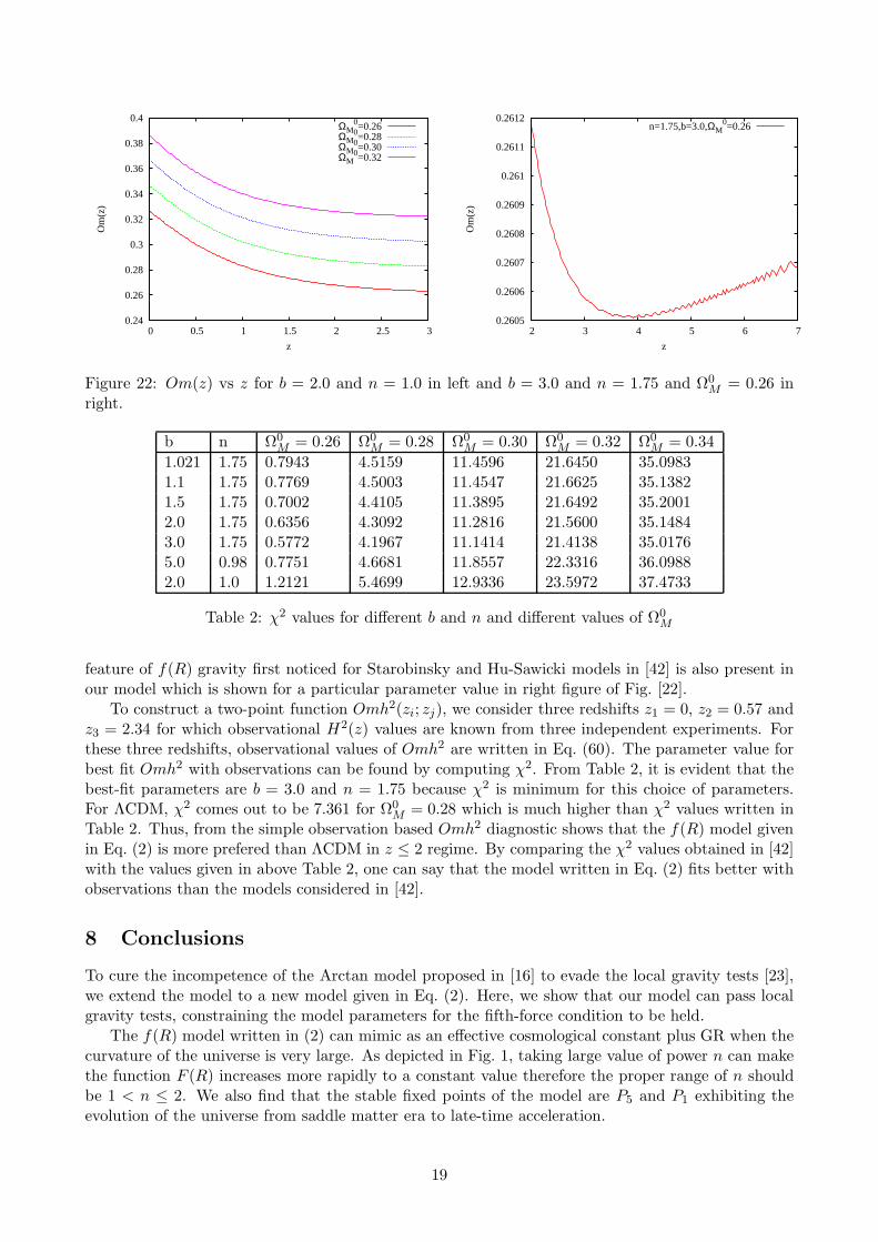
Through this Om diagnostic, we can detect the distinguishability of f(R) model from ΛCDM. Inaddition to this, we can pull the best choice of parameter values which fit well with the observationsby calculating χ2 values of two-point relations Omh2. To acquire the theoretical Omh2(zi; zj), oneneeds to solve the cosmological evolution equations and fetch the values of H at different z for agiven model. We establish the cosmological evolution equations (46), (47), (48) and (49) and solvethem in the preceding section. Plugging the calculated values of H(z) in Eq. (57), we obtain thetheoretical values of Om(z). Here, we are interested in comparing Om(z) profile for different Ω0
M andtherefore we use different values of Ω0
M to solve the cosmological equations. In Figs. [20], [21], andleft of Fig. [22], Om(z) functions are plotted w.r.t. redshift z for different Ω0
M values for differentparameters listed in Table 1. It can be easily seen that value of Om(z) remains constant aroundz = 3 but at lower redshifts z < 2 the Om(z) increases as z decreases. This clearly indicates thedeviation from ΛCDM and implies that the universe explained by the model given in Eq. (2) behavesas ΛCDM for higher redshifts but deviates for z < 2 i.e. in late time epoch. The deviation growsmore for lower n and b being maximum for n = 1.75 and b = 1.021. We can also see that the typical
18
0.24
0.26
0.28
0.3
0.32
0.34
0.36
0.38
0.4
0 0.5 1 1.5 2 2.5 3
Om
(z)
z
ΩM0=0.26
ΩM0=0.28
ΩM0=0.30
ΩM0=0.32
0.2605
0.2606
0.2607
0.2608
0.2609
0.261
0.2611
0.2612
2 3 4 5 6 7
Om
(z)
z
n=1.75,b=3.0,ΩM0=0.26
Figure 22: Om(z) vs z for b = 2.0 and n = 1.0 in left and b = 3.0 and n = 1.75 and Ω0M = 0.26 in
right.
b n Ω0M = 0.26 Ω0
M = 0.28 Ω0M = 0.30 Ω0
M = 0.32 Ω0M = 0.34
1.021 1.75 0.7943 4.5159 11.4596 21.6450 35.09831.1 1.75 0.7769 4.5003 11.4547 21.6625 35.13821.5 1.75 0.7002 4.4105 11.3895 21.6492 35.20012.0 1.75 0.6356 4.3092 11.2816 21.5600 35.14843.0 1.75 0.5772 4.1967 11.1414 21.4138 35.01765.0 0.98 0.7751 4.6681 11.8557 22.3316 36.09882.0 1.0 1.2121 5.4699 12.9336 23.5972 37.4733
Table 2: χ2 values for different b and n and different values of Ω0M
feature of f(R) gravity first noticed for Starobinsky and Hu-Sawicki models in [42] is also present inour model which is shown for a particular parameter value in right figure of Fig. [22].
To construct a two-point function Omh2(zi; zj), we consider three redshifts z1 = 0, z2 = 0.57 andz3 = 2.34 for which observational H2(z) values are known from three independent experiments. Forthese three redshifts, observational values of Omh2 are written in Eq. (60). The parameter value forbest fit Omh2 with observations can be found by computing χ2. From Table 2, it is evident that thebest-fit parameters are b = 3.0 and n = 1.75 because χ2 is minimum for this choice of parameters.For ΛCDM, χ2 comes out to be 7.361 for Ω0
M = 0.28 which is much higher than χ2 values written inTable 2. Thus, from the simple observation based Omh2 diagnostic shows that the f(R) model givenin Eq. (2) is more prefered than ΛCDM in z ≤ 2 regime. By comparing the χ2 values obtained in [42]with the values given in above Table 2, one can say that the model written in Eq. (2) fits better withobservations than the models considered in [42].
8 Conclusions
To cure the incompetence of the Arctan model proposed in [16] to evade the local gravity tests [23],we extend the model to a new model given in Eq. (2). Here, we show that our model can pass localgravity tests, constraining the model parameters for the fifth-force condition to be held.
The f(R) model written in (2) can mimic as an effective cosmological constant plus GR when thecurvature of the universe is very large. As depicted in Fig. 1, taking large value of power n can makethe function F (R) increases more rapidly to a constant value therefore the proper range of n shouldbe 1 < n ≤ 2. We also find that the stable fixed points of the model are P5 and P1 exhibiting theevolution of the universe from saddle matter era to late-time acceleration.
19
We put the model in (2) under scrutiny to investigate the fifth-force constraints for the modelthrough chameleon mechanism. We find that the model can evade local gravity test for the parametervalues n ≥ 1.75 and b ≥ 1.021. These constraints on the parameter values give rise to constraint onthe value of corresponding de Sitter point which is βRd ≥ 2.4.
The existence of curvature singularity in the model in Eq. (2) is also investigated. We find thatthere may be finite probability for scalar field to hit the singularity due to the finite potential VJ atthe singular point during its evolution. As described in [8], the curvature singularity can be cured byadding R2 term to the Lagrangian.
We also derive the cosmological evolution equations for this model considering an FRW backgrounduniverse and solve them numerically. We obtain the oscillatory behavior of Ricci scalar R and Hubbleparameter H which becomes less pronounced with higher values of b. It is found that the model (2)provides sufficiently long matter dominated era and radiation era at larger redshifts similar to ΛCDMmodel. These results are reconciled with the predictions of fixed point analysis and nucleosynthesis.The equation of state of the f(R) component of the fluid wx for our model oscillates around phantomdivide w = −1. We also find that the luminosity distance and distance modulus obtained in ourmodel are not much different from ΛCDM model and also fit with the supernova data. On the otherhand, through Om diagnostic we find that the model given in Eq. (2) is distinguishable from ΛCDMat redshifts z < 2. In Om diagnostic analysis, our model emerges as a better fit with baryon acousticoscillation data than ΛCDM. Performing χ2 test, we obtain n = 1.75 and b = 3.0 as a best-fit choiceof parameters.
The distinguishability from ΛCDM and also the viability of any f(R) model can be better testedwith large-scale structure data. The recent redshift space distortion(RSD) data can put tighterconstraints on the model, but yet an available number of data points is very less to test viability ofany model in a definite manner. Thus, we conclude that the model given in Eq. (2) gives rise to thedark energy dominated era while having correct cosmic history to coincide with other cosmologicalobservations and also evade local gravity tests.
References
[1] A. G. Riess et al. [Supernova Search Team Collaboration], Astron. J. 116, 1009 (1998)[astro-ph/9805201]. S. Perlmutter et al. [Supernova Cosmology Project Collaboration], Nature 391,51 (1998) [astro-ph/9712212]. B. P. Schmidt et al. [Supernova Search Team Collaboration], Astro-phys. J. 507, 46 (1998) [astro-ph/9805200]. S. Perlmutter et al. [Supernova Cosmology ProjectCollaboration], Astrophys. J. 517, 565 (1999) [astro-ph/9812133]. A. G. Riess et al. [SupernovaSearch Team Collaboration], Astrophys. J. 607, 665 (2004) [astro-ph/0402512].
[2] A. Padilla, arXiv:1502.05296 [hep-th].
[3] A.D.Felice and S.Tsujikawa, Living Rev. Relativity, 13, (2010), 3.
[4] T. P. Sotiriou and V. Faraoni, Rev. Mod. Phys. 82, 451 (2010) [arXiv:0805.1726 [gr-qc]].
[5] A. Starobinsky, JETP Lett. 86, 157 (2007) [0706.2041]
[6] W. Hu and I. Sawicki, Phys. Rev. D 76, 064004 (2007) [arXiv:0705.1158 [astro-ph]].
[7] S. A. Appleby and R. A. Battye, Phys. Lett. B 654, 7 (2007) [arXiv:0705.3199 [astro-ph]].
[8] S. Appleby, R. Battye and A. Starobinsky JCAP 1006, 005 (2010) [astro-ph/0909.1737]
[9] S. Tsujikawa, Phys. Rev. D 77, 023507 (2008) [arXiv:0709.1391 [astro-ph]].
[10] P. Zhang, Phys. Rev. D 73, 123504 (2006) [astro-ph/0511218].
20

[11] G. Cognola, E. Elizalde, S. Nojiri, S. D. Odintsov, L. Sebastiani and S. Zerbini, Phys. Rev. D77, 046009 (2008) [arXiv:0712.4017 [hep-th]].
[12] V. Miranda, S. E. Joras, I. Waga and M. Quartin, Phys. Rev. Lett. 102, 221101 (2009)[arXiv:0905.1941 [astro-ph.CO]].
[13] E. V. Linder, Phys. Rev. D 80, 123528 (2009) [arXiv:0905.2962 [astro-ph.CO]].
[14] K. Bamba, C. Q. Geng and C. C. Lee, JCAP 1008, 021 (2010) [arXiv:1005.4574 [astro-ph.CO]].
[15] K. Bamba, C. Q. Geng and C. C. Lee, Int. J. Mod. Phys. D 20, 1339 (2011) [arXiv:1108.2557[gr-qc]].
[16] S. I. Kruglov, Phys. Rev. D 89, no. 6, 064004 (2014) [arXiv:1310.6915 [gr-qc]].
[17] L. Amendola, R. Gannouji, D. Polarski and S. Tsujikawa, Phys. Rev. D 75, 083504 (2007)[gr-qc/0612180].
[18] S. Carloni, JCAP 1509, no. 09, 013 (2015) [arXiv:1505.06015 [gr-qc]].
[19] S. Kandhai and P. K. S. Dunsby, arXiv:1511.00101 [gr-qc].
[20] G. J. Olmo, Phys. Rev. D 72, 083505 (2005) [gr-qc/0505135].
[21] G. J. Olmo, Phys. Rev. Lett. 95, 261102 (2005) [gr-qc/0505101].
[22] C. M. Will, Living Rev. Rel. 17, 4 (2014) [arXiv:1403.7377 [gr-qc]].
[23] K. Dutta, S. Panda and A. Patel, arXiv:1601.07928 [gr-qc] (accepted for publication in PRD).
[24] S. A. Appleby and R. A. Battye, JCAP 0805, 019 (2008) [arXiv:0803.1081 [astro-ph]].
[25] A. Frolov, Phys. Rev. Lett. 101, 061103 (2008) [astro-ph/0803.2500]
[26] K. Dutta, S. Panda and A. Patel, Phys. Rev. D 92, no. 6, 063503 (2015) [arXiv:1504.05790[gr-qc]].
[27] S. Nojiri and S. D. Odintsov, Phys. Rev. D 78, 046006 (2008) [arXiv:0804.3519 [hep-th]].
[28] K. Bamba, S. Nojiri and S. D. Odintsov, JCAP 0810, 045 (2008) [arXiv:0807.2575 [hep-th]].
[29] A. Dev, D. Jain, S. Jhingan, S. Nojiri, M. Sami and I. Thongkool, Phys. Rev. D 78, 083515(2008) [hep-th/0807.3445].
[30] I. Thongkool, M. Sami, R. Gannouji and S. Jhingan, Phys. Rev. D 80, 043523 (2009)[arXiv:0906.2460 [hep-th]].
[31] S. Capozziello, M. De Laurentis, S. Nojiri and S. D. Odintsov, Phys. Rev. D 79, 124007 (2009)[arXiv:0903.2753 [hep-th]].
[32] A. de la Cruz-Dombriz, P. K. S. Dunsby, S. Kandhai and D. Saez-Gomez, Phys. Rev. D 93, no.8, 084016 (2016) [arXiv:1511.00102 [gr-qc]].
[33] E. Arbuzova, S. Dolgov, Phys. Lett. B 700, 289 (2011) [astro-ph/1012.1963]
[34] C. Lee, C. Geng and L. Yang, Prog. Theor. Phys. 128, 415 (2012) [astro-ph/1201.4546].
[35] L. Reverberi, Phys. Rev. D 87, 084005 (2013) [gr-qc/1212.2870]
[36] T. Kobayashi and K. i. Maeda, Phys. Rev. D 78, 064019 (2008) [arXiv:0807.2503 [astro-ph]].
21

[37] A. Upadhye and W. Hu, Phys. Rev. D 80, 064002 (2009) [arXiv:0905.4055 [astro-ph.CO]].
[38] E. Babichev and D. Langlois, Phys. Rev. D 81, 124051 (2010) [arXiv:0911.1297 [gr-qc]].
[39] A. Shafieloo, V. Sahni and A. A. Starobinsky, Phys. Rev. D 86, 103527 (2012) [arXiv:1205.2870[astro-ph.CO]].
[40] V. Sahni, A. Shafieloo and A. A. Starobinsky, Phys. Rev. D 78, 103502 (2008) [arXiv:0807.3548[astro-ph]].
[41] V. Sahni, A. Shafieloo and A. A. Starobinsky, Astrophys. J. 793, no. 2, L40 (2014)[arXiv:1406.2209 [astro-ph.CO]].
[42] L. G. Jaime, Phys. Rev. D 91, no. 12, 124070 (2015) [arXiv:1506.03618 [gr-qc]].
[43] R. C. Nunes, S. Pan, E. N. Saridakis and E. M. C. Abreu, arXiv:1610.07518 [astro-ph.CO].
[44] L. G. Jaime, L. Patino and M. Salgado, arXiv:1206.1642 [gr-qc].
[45] R. Amanullah, et al. (Supernova Cosmology Project), Astrophys. J. 716, 712 (2010)
[46] J. Khoury and A. Weltman, Phys. Rev. Lett. 93, 171104 (2004) [astro-ph/0309300]; J. Khouryand A. Weltman, Phys. Rev. D 69, 044026 (2004) [astro-ph/0309411].
[47] S. Capozziello, S. Tsujikawa, Phys. Rev. D 77, 107501 (2008) [gr-qc/0712.2268]
[48] P. A. R. Ade et al. [Planck Collaboration], Astron. Astrophys. 571, A16 (2014) [arXiv:1303.5076[astro-ph.CO]].
[49] L. Samushia et al., Mon. Not. Roy. Astron. Soc. 429, 1514 (2013) [arXiv:1206.5309 [astro-ph.CO]].
[50] L. Anderson et al., Mon. Not. Roy. Astron. Soc. 441, 24 (2014)
[51] T. Delubac et al. [BOSS Collaboration], Astron. Astrophys. 574, A59 (2015) [arXiv:1404.1801[astro-ph.CO]].
[52] G. Efstathiou et al., Mon. Not. Roy. Astron. Soc. 440, 1138 (2014)
22