NBER WORKING PAPER SERIES

YESTERDAY'S HEROES:COMPENSATION AND CREATIVE RISK-TAKING

Ing-Haw ChengHarrison Hong

Jose A. Scheinkman

Working Paper 16176http://www.nber.org/papers/w16176

NATIONAL BUREAU OF ECONOMIC RESEARCH1050 Massachusetts Avenue

Cambridge, MA 02138July 2010

We thank Jeremy Stein, Rene Stulz, Luigi Zingales, Steven Kaplan, Tobias Adrian, Sule Alan, AugustinLandier,Terry Walter, Bob DeYoung, Ira Kay, Yaniv Grinstein, Patrick Bolton, Marco Becht andparticipantsat the Princeton-Cambridge Conference, SIFR Conference,HEC, NBER, University of Michigan,Universityof Technology at Sydney, Chinese University of Hong Kong, CEMFI, LSE, Universityof Kansas SouthwindConference, Federal Reserve Bank of New York, Columbia University,ECGI-CEPR-IESE MadridConference, University of Florida, 2011 AFA Meetings, Federal Reserve Bank of Chicago 47 AnnualConference on Banking, and the NBER Conference on Market Institutionsand Financial Market Riskfor helpful comments.The views expressed herein are those of the authorsand do not necessarily reflectthe views of theNational Bureau of Economic Research.

NBER working papers are circulated for discussion and comment purposes. They have not been peer-reviewed or been subject to the review by the NBER Board of Directors that accompanies officialNBER publications.

© 2010 by Ing-Haw Cheng, Harrison Hong, and Jose A. Scheinkman. All rights reserved. Short sectionsof text, not to exceed two paragraphs, may be quoted without explicit permission provided that fullcredit, including © notice, is given to the source.

Yesterday's Heroes: Compensation and Creative Risk-TakingIng-Haw Cheng, Harrison Hong, and Jose A. ScheinkmanNBER Working Paper No. 16176July 2010, Revised June 2011JEL No. G01,G21,G22,G24,G32

ABSTRACT

We study the relationship between compensation and risk-taking among finance firms using a neglected insight from principal-agent contracting with hidden action and risk-averse agents.If the sensitivity of pay to stock price or slope does not vary with stock price volatility, then total compensation has to increase with firm risk to satisfy as agent's individual rationality constraint. Consistent with this hypothesis, we find a correlation between total executive compensation, controlling for firm size, and risk measures such as firm beta, return volatility, and exposure to theABX sub-prime index. There is no relationship between insider ownership, a proxy for slope, andthese measures. Compensation and firm risk are not related to governance variables. They increasewith institutional investor ownership, which suggests that heterogeneous investors incentivize firms to take varying levels of risks. Our results hold for non-finance firms and point to newprincipal-agent contracting empirics.

Ing-Haw ChengRoss School of BusinessUniversity of Michigan701 Tappan StAnn Arbor, MI 48109ingcheng@umich.edu

Harrison HongDepartment of EconomicsPrinceton University26 Prospect AvenuePrinceton, NJ 08540and NBERhhong@princeton.edu

Jose A. ScheinkmanDepartment of EconomicsPrinceton UniversityPrinceton, NJ 08544-1021and NBERjoses@princeton.edu

1

I. Introduction

Many blame Wall Street compensation for the most significant economic crisis since the Great

Depression. In his testimony (June 6, 2009) in front of Congress on the Treasury budget, Secretary

Geithner argues, “I think that although many things caused this crisis, what happened to compensation

and the incentives in creative risk taking did contribute in some institutions to the vulnerability that we

saw in this financial crisis” (emphasis added). To address this issue, the US has promoted reforms to tie

pay to long-term performance and increase the say of shareholders in approving compensation and

electing directors on compensation committees.1 Implicit in this view is that finance firms’ short-termist

incentives reflect mis-governance or entrenchment and a misalignment with shareholder interest.

In this paper, we consider an alternative perspective---namely, investors of some firms very

much wanted and compensated their managers to take creative risks. In his interview with the Financial

Times back in July 2007, Chuck Prince, then CEO of Citigroup, in referring to his company not backing

away from risks at the beginning of the subprime crisis, remarked: “When the music stops, in terms of

liquidity, things will be complicated. But as long as the music is playing, you've got to get up and

dance. We're still dancing.” This quote is often attributed as market pressure (presumably being fired

by impatient shareholders) forcing Citi’s managers to take on such risks, whether or not they fully

understood them. In other words, the short-termism emanated not so much from mis-governance or

entrenchment as from demand on the part of investors themselves.2

As such, we examine the relationship between compensation and risk taking through the lens of a

classical optimal contracting framework between a principal and a risk-averse agent. The principal in

our context is the shareholders and the agent is the CEO or other top managers. The well-analyzed

prediction of this model is that firms with more volatile stock prices should optimally give risk-averse

managers less exposure (or slope) to stock returns in the incentive scheme, typically measured by insider

ownership stakes. It is well known that there is a weak relationship between slope and stock price

volatility among a panel of firms from different industries; if anything, the relationship is positive.

There are many reasons for why this could be true in the principal-agent setting (see Prendergast, 1999 1 The view that short-termism contributed to the crisis is shared by other governments, particularly in the UK, where a parliamentary committee investigating the crisis “found that bonus-driven remuneration structures encouraged reckless and excessive risk-taking and that the design of bonus schemes was not aligned with the interests of shareholders and the long-term sustainability of the banks.” (UK House of Commons, 2009) 2 This more nuanced perspective of a short-term stock market forcing management to be excessively myopic also has basis in theory (see Stein, 1989 and Stein, 2003 for a review of this large literature on the contrasting perspectives of the source of short-termism in markets).

2

and Prendergast, 2000 for reviews). Notably, managers’ hidden actions may be more important in high

volatility firms, and hence insider ownership stakes need not decrease with firm risk, and may actually

increase.

In contrast, we study the relationship between compensation and risk-taking among finance

firms using a neglected insight from principal-agent contracting with hidden actions and risk-averse

agents. If the sensitivity of pay to stock price (the incentive slope) does not vary with stock price

volatility for whatever reason, then total compensation has to increase with firm risk to satisfy an agent’s

individual rationality constraint. That is, when the optimal incentive slope does not vary with the stock

price volatility, a riskier firm must pay more than a less risky firm to attract the same managerial talent.

This is shown below in the linear contract set-up of Holmstrom and Milgrom (1987), but the

point is a robust one simply emanating from the risk aversion of agents and their participation constraint.

Indeed, recent models of managerial incentives also emphasize the individual rationality constraint and

deliver a similar prediction that high risk firms pay higher wages for various reasons, including disutility

of effort, efficiency wages or rent seeking.3 Our contribution is to point out that empirical work has

ignored the individual rationality constraint in favor the incentive compatibility constraint and to show

that important information can be obtained from considering the two simultaneously.

Using data on executive compensation for finance firms from 1990-2008, we find strong support

for models of managerial incentives which predict a strong relationship between total pay and firm price

volatility and a weak relationship between incentive slopes and total pay.

We then go on to develop further corroborating evidence by showing that high compensation and

risk-taking are correlated with higher institutional ownership. In contrast, compensation and risk-taking

are not related to governance variables. Contrary to the prevailing wisdom that managerial

entrenchment or a failure of governance led finance firms to take excessive risk, we argue instead that

these findings suggest that investors with heterogeneous risk preferences incentivize firms to take

different levels of risk.

3 In the equilibrium model in Edmans and Gabaix (2011), the strength of incentives given to managers depends only on the disutility of effort and is independent of firm’s risk or the agent’s risk aversion. As a result, expected total pay to a risk-averse manager increases with the riskiness of the firm. In their model, better managers are assigned to larger firms, so total pay of a manager also depends on firm size. See also Peng and Roell (2009) for a model that can generate similar predictions. Axelson and Bond (2010) gives a similar prediction using an efficiency wage or rent mechanism in which higher risk firms pay more, which they argue better match the empirical findings regarding the career of investment bankers as captured in Oyer (2008). These equilibrium considerations magnify risk aversion effects even if the risk aversion effects might not be large to begin with (Kaplan and Stromberg, 2004).

3

Because of our focus on the individual participation or rationality constraint (IR) rather than the

individual incentive compatibility constraint (IC), we develop different measures of compensation than

the literature. The literature’s focus on the IC has led to careful study of inside ownership stakes. But

insider ownership stakes reflect not just the compensation practice of a firm but also the portfolio choice

of the manager. If overconfident managers are more likely to work for very volatile firms and these

managers are more likely to keep sub-optimally undiversified or large stakes, then this might bias

finding the predicted IC relationship that insider stakes should be lower in more volatile firms.4 Rather,

we use the total flow pay granted each year to the top insiders. These payouts better reflect the

compensation practice of the firm. More specifically, we look at total executive compensation adjusting

for a firm’s market capitalization or size, since better managers work for more valuable firms (see, for

instance, the matching theory of Gabaix and Landier, 2008). We want to purge out quality differences

in managers and firms with a careful firm size control throughout our analysis.

We establish the following findings. First, there is substantial cross-sectional heterogeneity in

residual total executive compensation, which is defined as the total pay of managers controlling for firm

size and finance sub-industry. The residual compensation measure obtained from this regression is

highly persistent and is a firm-specific characteristic. Firms with persistently high residual compensation

include Bear Stearns, Lehman, Citicorp, Countrywide, and AIG. Low or moderate residual

compensation firms include Wells Fargo and Berkshire Hathaway. Firm risk measures, including market

beta, stock price volatility and firm exposure to the ABX sub-prime index, are also highly persistent.

We use an assortment of risk measures to capture the heterogeneous ability or inclination of

finance firms to engage in creative risk taking. For instance, a firm’s propensity to effectively sell out of

the money puts or insurance on the stock market (i.e., to engage in tail risk) may not be entirely captured

by stock price volatility. Ex post market betas in this instance may better capture a firm engaging in tail

risk since the firm is fine when the market does well and goes bust when the market does poorly. A

firm’s stock price exposure to the ABX directly captures its exposure to the subprime housing market.

In this sense, we go beyond the exercise of relating compensation to return volatility in order to better

capture finance firms’ creative risk-taking. Additionally, for finance firms, price risk measures far

outperform book measures since they often engage in off-balance sheet transactions in creating their

creative and systematic risk profiles.

4 Indeed, Malmendier and Tate (2005) and Malmendier and Tate (2008) provide evidence that managerial overconfidence as measured by their portfolio holdings and external press portrayals influence investment and acquisition choices.

4

Second, we find that, although insider ownership stakes are not correlated with firm riskiness,5

our residual compensation measure is strongly correlated with these price-based measures of risk,

consistent with our hypothesis regarding the individual rationality constraint. Firms with high executive

compensation have a higher market beta, higher return volatility, and ABX exposure. For instance, a

one-standard deviation increase in stock price exposure to price movements in the ABX net of size and

finance sub-industry is associated with a 0.33-standard deviation increase in residual compensation. A

price-based risk score, defined as the average of the normalized z-scores of market beta, return volatility

and ABX exposure, is even more strongly related to residual compensation than any of the measures

individually.

Not surprisingly, firms with high residual compensation, since they have higher beta and are

more volatile, are more likely to be in the tails of performance, with extremely good performance when

the market did well and extremely poor performance when the market did poorly. For example, a one-

standard deviation increase in residual compensation in 1998-2000 is associated with 21% lower returns

over the market in the 2001-2008 period. These results stand in contrast to more traditional book-based

measures of risk-taking, which do less well. This is perhaps not surprising since many of the finance

firms’ exposures during the recent crisis were off balance sheet.

These findings suggest that there is substantial heterogeneity among financial firms in which

high-compensation and high risk-taking go hand in hand. As a result, the aggressive firms that were

yesterday’s heroes when the stock market did well can easily be today’s outcasts when fortunes reverse,

very much to the point of what we have experienced in the last twenty or so years. The important thing

to note here is that our price risk score measure is robust and statistically significant across all sub-

industries of finance including broker dealers, banks and insurance companies. Our findings are also

robust to a series of other checks.

We then relate residual total compensation and firm riskiness to governance or entrenchment

measures. We find that standard governance measures such as the Gompers, Ishii and Metrick (2003)

and Bebchuk, Cohen and Ferrell (2009) measures of entrenchment, as well as board independence, are

not correlated with our results. So it appears that there is little evidence of mis-governance using these

5 Fahlenbrach and Stulz (2010) find that finance firms with higher insider ownership stakes had poorer performance during the crisis, suggesting little relationship between insider ownership and firm risk. Keys, Mukherjee, Seru and Vig (2009) also find little evidence that CEO incentives affected loan quality. Mehran and Rosenberg (2008) show stock option grants lead CEOs to take less borrowing and higher capital ratios but to undertake riskier investments. Laeven and Levine (2009) find that bank risk is higher among banks that have large owners with substantial stakes.

5

standard metrics for mis-alignment of interest between shareholders and management, at least in the

cross-section.

In contrast, we find that residual compensation and risk-taking are positively correlated with

institutional ownership. The presumption, given that institutional investors are sophisticated, is that the

incentives provided were consistent with optimal contracts and shareholder preferences. The

institutional ownership finding suggests that there is heterogeneity in investor preferences with

institutional investors wanting certain firms to take more risks and hence having to give them incentives

to do so (Froot, Perold and Stein, 1992; Bolton, Scheinkman and Xiong, 2006). Indeed, both anecdotal

and empirical evidence suggests that institutional investors are the ones with the power to pressure

management (Graham, Harvey and Rajgopal, 2005; Parrino, Sias and Starks, 2003). Of course, one has

to be careful in interpretations here. If institutional investors are too short-termist and always flip the

shares of the company, then they will not have any influence over management. But in practice, there is

plentiful evidence that institutional investors care greatly about companies making quarterly earnings

targets, presumably because the accompanying growth in share prices helps the institutional investors’

portfolio performance. Our analysis here builds on the Hartzell and Starks (2003) analysis of the key

role of institutional investors in providing incentives.

We stress that we do not view this hypothesis as incompatible with the hypothesis that

entrenchment is a significant problem that led to the crisis. But in light of the non-correlation between

shareholder rights and both risk-taking and price performance, our results at a minimum suggest that

further research should explore investor preferences as an alternative hypothesis to failures of

governance.

We focus on finance firms since we are better able to address unobserved heterogeneity by

conditioning our analysis within sub-industries of finance. However, our insights apply more broadly to

other firms. To this end, we extend our analysis to non-financial firms. We find similar results, though

we are less confident in the interpretation since there is much more heterogeneity in this sample.

Nonetheless, it appears that our insight regarding the relationship between total pay and stock price

volatility holds generally. Hence, our paper points to a need to refocus empirical strategies in the

principal-agent contracting literature.6

6 Oyer (2004) also shows the way on the importance of looking at IR constraints. He shows that, if an agent’s outside option is positively correlated with the market, then it might make sense to incentivize the manager with systematic risk.

6

Our paper is organized as follows. We present a simple model in Section II to motivate our

empirical analysis and the data in Section III. We present the results in Section IV and conclude with

some thoughts on future research in Section V.

II. Model

Our simple model highlights the prediction of the classical principal-agent model that

equilibrium total compensation must increase with firm risk to satisfy an agent’s participation constraint

when the sensitivity of pay to stock price (the incentive slope) does not vary with stock price risk.7

While we focus on the classical set-up for expositional reasons, one can obtain similar conclusions using

more recent dynamic and equilibrium managerial incentive models highlighted in the introduction.

Consider a firm whose output is a linear function of an agent’s effort, a, and Gaussian noise, ̃~N(0, ): = ℎ + ̃ The parameter h reflects the agent’s marginal productivity of effort, which may be a function of the risk

of the firm, , as well as other sources of heterogeneity. The agent cares about their total pay less a

positive, increasing, convex cost of supplying effort, ( ), with (0) = 0, and has exponential utility

with constant absolute risk aversion . Effort is unobserved to the principal, but all other parameters are

common knowledge. If we let ( ) = + denote a linear sharing rule between the principal and

the agent, this implies that the agent maximizes

+ ℎ − ( ) − 2

Optimal effort is governed by the incentive compatibility constraint, which requires ( ) = ℎ

Participation requires that the expected utility equals the agent’s reservation utility :

≡ ( ) = + ℎ = + ( ) + 2

7 The reasons why the incentive slope may not move with volatility are varied. For example, Prendergast (2000) notes that whether the slope increases or decreases depends on the nature of the uncertainty and whether inputs may be easily monitored.

7

The principal maximizes output net of payments to the agent subject to these two constraints,

which leads to the familiar equilibrium piece rate,

∗ = 11 + ′′( ∗)/ℎ

Our insight is that, if the equilibrium piece rate is insensitive to changes in the risk, then the expected

total compensation must increase with the risk; that is, if ∗/ = 0, then ∗/ > 0. This

situation arises in our model when the marginal productivity of the agent is positively correlated with the

risk of the firm. For example, one may conjecture that for risky firms like Bear Stearns, traders have a

higher marginal impact on outcomes.

For concreteness, consider the classic case where the cost of effort is quadratic, ( ) = /2. A

necessary and sufficient condition for ∗/ = 0 is then ℎ/ℎ/ = 12

If the elasticity of the marginal productivity of effort with respect to output variance is one-half, then we

expect equilibrium incentive slopes not to vary with observed risk. High risk firms are also high

productivity firms, and although it is optimal to incentivize the manager to work hard at these firms

through a higher slope , the higher risk tempers this in equilibrium.

More generally, whenever ∗/ = 0, then, for a wide range of effort disutility functions c,

total dollar compensation must rise with , for two reasons. First, from the participation constraint,

the principal must compensate the risk-averse agent more from a classical insurance motive. (If ∗/ < 0, this may not hold in equilibrium since the equilibrium slope may fall as firm risk rises.)

Second, the principal needs to compensate the agent to work harder at the high marginal productivity

firm. Formally, we have the following proposition:

Proposition. Suppose the disutility of effort satisfies > 0, > 0, and < 2 for a > 0. If = 0, then > 0 and > 0.

Proof: See the Appendix. Note that the condition on the cost function c is satisfied by every =

for > 1, > 0 and also every exponential function of the form = exp( ) with > 0. ■

8

Our simple model highlights the fact that any test of the principal-agent theory must be a joint

test of both the incentive constraint and the participation constraint. The often-neglected participation

constraint can offer additional empirical insight when the incentive slope appears insensitive to the risk

of the firm. (The proposition generalizes to the case where ∗/ ≥ 0, with the additional

assumption that ( ) ≥ 0.) This is the empirical implication that we examine in this paper.

Our strategy is to relate size and industry-adjusted measures of total compensation T and slope to

ex post realizations of risk. Adjusting for size and industry is important since the prediction of the

model only holds for firms of equal scale or capital. We proxy for the scale of a firm using the market

capitalization of its equity. We would also like to obtain a measure of T, the total dollar compensation

paid to the manager. We focus on the total level of flow compensation to the manager. Intuitively,

measuring the flow pay to the manager best captures compensation practices of the principal, which is

the spirit of the IR constraint. While another potential measure could be the dollar value of the

manager’s accumulated stake in the firm, this is potentially contaminated by the manager’s individual

portfolio decisions and hence could be subject to managerial behavioral biases (Malmendier and Tate,

2005). Alternatively, one can think of the flow compensation as a proxy for the total pay received in

annuity over the tenure of the manager.

We also verify in our data that slope is insensitive to risk. We use the effective percentage

ownership as a measure of slope incentives as this is the closest proxy for in our model. Jensen and

Murphy (1990) use effective inside ownership as a measure of incentives. One concern is that different

measures of incentives may be appropriate under alternative assumptions. Baker and Hall (2004) and

Hall and Liebman (1998) suggest using the market value of insider equity as a measure of incentives.

We verify in our data that alternative measures of incentives also have a non-negative relationship with

risk.

In order to capture the complex risk profiles of financial firms, we go beyond the practice of

relating compensation to return volatility and relate compensation to not only volatility, but also a firm’s

market beta and stock price exposure to movements in the ABX subprime index. The idea is that these

other measures may capture additional risks that managers face. For example, a high tail-risk strategy

such as selling out of the money puts on the stock market is inherently a high beta strategy. At financial

firms, these risk profiles may also be influenced by managerial hidden actions, and thus managers would

need to be compensated for these risks. For example, in our model, one can interpret the managerial

9

action a as selling these out of the money puts.8 As we will show, compensation is strongly related to

individual measures of risk as well as our price risk score.

III. Empirical Methodology

A. Classifying Financial Firms

Our sample consists of financial firms in the intersection of ExecuComp and the CRSP-

COMPUSTAT Annual file, 1992-2008. We identify three groups of financial firms. We first construct

a group of primary dealers by hand-matching a historical list from the Federal Reserve Bank of New

York with PERMCOs from our CRSP file. When a primary dealer is a subsidiary of a larger bank

holding company in CRSP, we group the bank holding company with the primary dealers.

We then use SIC codes to classify firms into a second group of banks, lenders, and bank-holding

companies which do not have primary dealer subsidiaries. According to the US Department of Labor

OSHA SIC Manual, this group comprises firms from SIC 60 commercial banks, SIC 61 non-deposit

lenders, and SIC 6712 bank holding companies. Our third and last group of financial firms are insurers

from SIC 6331 (fire, marine and casualty insurance) and SIC 6351 (surety insurance). This group of

insurers contains firms such as AIG and monoline insurers such as MBIA.

Our data on SIC codes comes from both CRSP and COMPUSTAT. We include a firm as a

financial firm if either its CRSP or COMPUSTAT SIC code indicates it is a financial firm. However, a

number of the SIC codes obtained from CRSP and COMPUSTAT do not exactly match the SIC

classification in the SIC Manual, particularly for bank holding companies. For example, Countrywide

(PERMCO 796) and AMBAC Financial (PERMCO 29052) have SIC 6711 and 6719 in CRSP,

respectively. We worry that we might have misclassified some financial firms. We supplement this list

by hand collecting additional financial firms from the more expansive three-digit SIC codes of 670 and

671 and then looking at company description via 10-K statements on EDGAR. We conduct a similar

check for three-digit SIC codes 633 and 635. Finally, we hand check all the firms on our list to make

sure we have not included any non-financials. We also exclude Fannie Mae, Freddie Mac, and Sallie

Mae from our analysis since they are effectively government enterprises. Our baseline sample of

financial firms has to have data from all three of these databases.

8 Strictly speaking, in our simple model, the parameter is exogenous. However, Edmans and Gabaix (2011) show that if the manager may control risk itself, incentives may be increasing in risk. Thus a similar insight applies: total compensation must increase with risk. Additionally, Oyer (2004) shows that if managers’ outside options are correlated with market movements, then tying compensation to systematic risk may be optimal.

10

B. Cross-Sections and Variable Definition

Our goal is to relate heterogeneity in compensation practices at finance firms to heterogeneity in

their ex post realizations of risk within the cross-section. To this end, we split our sample into two

periods—an early period defined as 1992 (when we start having reasonable executive compensation

data) up to 2000, which marks the end of the dot-com era and a late period from 2001-2008 which marks

the beginning and end of the housing boom. We then take 1992-1994 (1998-2000) to create a ranking of

executive compensation among firms at the end of 1994 (2000). As we will show, compensation

practices are highly persistent across time, which makes our approach very conservative compared to a

pooled panel analysis. Additionally, this persistence implies that the variation in compensation practices

we are exploiting is essentially a firm fixed-effect, making a “within-firm” analysis inappropriate. Our

choice of sample split is simply designed to give us a long period over which the market rose and

another long period over which the market fell. In fact, the relationship between compensation practices

and risk is even stronger in a pooled panel analysis, which we show in the robustness section.

We measure total flow compensation by averaging the total direct compensation (TDC1 in

ExecuComp) across the top five executives at each firm, and we label this variable Executive

Compensation.9 Total direct compensation includes bonus, salary, equity and option grants, and other

forms of annual compensation. We exclude pay in years associated with IPOs since pay during those

periods often involve one-time startup stock grants that are less relevant for persistent compensation

practices. We measure Inside Ownership as the total effective number of shares owned by the top five

executives, where we include delta-weighted options using the method described in Core and Guay

(1999), divided by the total number of shares outstanding.

We compute Market Capitalization in a year as shares outstanding (SHROUT) times price (PRC)

as of the fiscal year-end month (summed up over all classes of stock) from CRSP. The market-to-book

ratio is Market Capitalization divided by book equity (stockholders equity plus deferred taxes and

investment tax credits, less the book value of preferred stock, from COMPUSTAT). We measure

leverage as Total Book Assets (AT) divided by Stockholders Equity (SEQ), following Adrian and Shin

(2009). We think of these variables as sources of heterogeneity in compensation practices, and each of

these variables is accordingly averaged over the ranking period.

9 Firms occasionally report the compensation of more than five people, in which case we take the top five highly paid executives. Occasionally, firms report compensation of fewer than five people as well. Because firms who report less than five executives may not be strictly comparable to firms who report compensation of the top five (the vast majority of the sample), we also re-do our analysis using top 5 compensation only when five executives report compensation. Results are very similar.

11

We compute three measures of ex post realizations of risk: 1) the beta of the firm’s stock (Beta),

2) the firm’s stock return volatility (Return Volatility), 3) the correlation of a firm’s daily stock returns

with returns to the ABX AAA index (Exposure to ABX). We compute a firm’s Market Beta and Return

Volatility for a given period (1995-2000 in the early period or 2001-2008 in the late period) using the

CRSP Daily Returns File, and take our market return to be the CRSP Value-Weighted Index return

(including dividends). Our data on the risk-free return comes from Ken French’s website. In computing

betas and volatility, we require at least one year’s worth of observations (252 trading days) in that

period. We report volatility in annualized terms, and we follow Shumway (1997) in our treatment of

delisting returns. For firms with dual-class stock such as Berkshire Hathaway, we compute our

measures of risk using a value-weighted set of returns.

We use the on-the-run ABX daily price index obtained from Barclays Capital Live to compute a

firm’s ABX exposure.10 Following Longstaff (2010), we compute the ABX return as the log of the

time-t price divided by the time t-1 price, where we ignore the coupon rates of each tranche (i.e.,

following Longstaff, 2010, we are assuming a coupon yield of zero). We compute a firm’s exposure to

the AAA tranche by regressing returns obtained from the CRSP Daily Returns File on returns to the

ABX AAA and returns to the market for each firm from when the ABX was created in 2006 through the

end of 2008. We take the coefficient on ABX returns as the firm’s Exposure to ABX.

We compute a price-based risk score measure that is an equal-weighted average of the

standardized z-scores of a firm’s Beta, Return Volatility and, in the late period, Exposure to ABX. As

previously discussed, a composite score can better capture many dimensions of firm risk important for

financial firms. Additionally, individual risk measures are noisy and hence averaging them provides a

cleaner measure of firm risk. This price-based risk score is our primary measure of ex post realizations

of risk.11 We measure firm outcomes by looking at a firm’s Cumulative Excess Return, defined as the

total buy-and-hold return of a firm’s stock over each period less the total buy-and-hold return of the

market.

We also relate these measures of compensation, risk and stock price performance to measures of

governance. We obtain from RiskMetrics data on corporate governance including the G index

(Gompers, Ishii and Metrick, 2003) and the percentage of directors that are outsiders (classified as

10 Barclays Capital Live, formerly known as Lehman Live, is available at http://live.barcap.com/ . The ABX indices are compiled and maintained by MarkIt, at http://www.markit.com/ . Longstaff (2010) provides a discussion of the index. 11 Our price-based risk score is also motivated by a principal components analysis of Market Beta, Return Volatility and Exposure to ABX. The first principal component explains over 70% of the variation in the three measures and has loadings very close to an equal-weighted average.

12

“Independent” by RiskMetrics). Since the RiskMetrics data on directors goes back to 1997, we have

data on independence only for our late period. We obtain data on the Entrenchment Index (Bebchuk,

Cohen and Ferrell, 2009) from Lucian Bebchuk’s website.

We obtain data on institutional ownership from the Thomson Reuters S34 database, which

captures 13F filings by financial institutions electronically. We match 8-digit CUSIPs in Thomson to

PERMNOs in CRSP, noting that the CUSIPs in Thomson are provided for the filing date (not the

reporting date). For each PERMNO, we divide the shares held by each financial institution (SHARES)

by the shares outstanding (as reported by Thomson in SHROUT1 before 1999 and SHROUT2 after

1999) and sum up over each stock. We take care to ensure that holdings and shares outstanding both

reflect stock splits when necessary.12 We censor the percentage of shares held by institutions at 1 for a

few observations.

C. Adjusting for Size and Industry

Within each cross section that we work with, we adjust total compensation for firm size and

finance sub-industry, since the theory speaks to compensation practices netted out of these factors. We

adjust for firm size since it is well known that the best personnel work for the biggest firms (Gabaix and

Landier, 2008; Murphy, 1999), and we adjust for finance sub-industries since each sub-industry may

have different compensation practices.13

Ideally, we would like to control for heterogeneity by allowing both slopes and intercepts to vary

across sub-industries. Unfortunately, the limited number of primary dealers per year does not allow us

to form reliable estimates of the slope and intercept within that group.14 Instead, we take the log of

average executive compensation in 1992-1994 (1998-2000 in the late period) and regress it on the log of

firms’ average market capitalization during the same period, allowing intercepts to vary by sub-industry

and allowing the insurers group to have a slope distinct from banks and primary dealers. This

12 We always divide shares held by the Thomson-provided value of shares outstanding rather than the CRSP value of shares outstanding to avoid mis-computing institutional ownership due to misalignments between when Thomson and CRSP report splits. When Thomson reports multiple filings, we always take the first filing, which corrects for the fact that shares outstanding may have changed by a later filing. There is one instance where Thomson’s value of shares outstanding (SHROUT2) does not make any sense, for Independence Community Bank (PERMNO 85876) in 1998Q3. Here we replace that value with the CRSP value of shares outstanding. 13 Murphy (1999) documents that there is substantial heterogeneity in how pay scales with size across non-financial industries. We view our three groups as a rough split among firms that engage in investment banking and intensive trading activity, other banks that operate more as commercial banks and lenders, and, finally, financial insurers. 14 In particular, the estimate of the slope of compensation and market capitalization fluctuates depending on the year in which the regression is run due to changes in the composition of the primary dealer group. Consistent with this, running a regression that allows for slopes and intercepts to vary across all sub-industries yields a large standard error on the slope for primary dealers.

13

specification allows for heterogeneity in the levels of pay across sub-industries and for an insurer-

specific slope (where we have enough observations to form a reliable estimate).

Our measure of compensation practices is the residual of each one of these regressions, which we

term Residual Compensation, and which captures firm compensation practices net of firm size and

industry factors. Our approach necessarily emphasizes the cross-sectional distribution of such practices,

and we relate these measures to ex post realizations of risk described above. We emphasize ex post

realizations of risk since in principle the compensation that principals pay should align with the risk of

future outcomes expected ex ante. Our analysis thus implicitly assumes rational expectations on the part

of the principal.

Specifically, we regress residual compensation from 1992-1994 on risk measures computed

using data from 1995-2000. We perform a similar exercise using residual compensation from 1998-

2000 and risk measures from 2001-2008. During the late period, our price risk score includes the

sensitivity of a firm’s stock price to the ABX subprime index. To the extent that high residual

compensation firms are high risk firms, we expect these firms to have done the best when the market

was up (the early period) and done the worst when the market was down (the late period). To this end,

we also look at the correlation between residual compensation and cumulative return performance.

We adjust all variables in our analysis, including inside ownership, risk measures, and

governance measures, symmetrically. In other words, variables in our regressions are residuals, which

we winsorize at the 1 and 99% levels. Econometrically, our regression results are nearly equivalent to

regressing unadjusted compensation variables on unadjusted risk variables while including a set of size

and industry controls described above. However, given that sample compositions vary when we look at

different measures of risk and governance, our approach has the advantage of maintaining a constant

residual compensation ranking relative to the case where size controls are included separately in each

regression. For example, we only have data on the G Index for a subset of our firms. If sample

compositions did not vary, the two approaches would be exactly equivalent. We also believe residual

compensation has a natural economic intuition of pay netted out for industry and size, which most

appropriately matches the prediction we are trying to test from the theory. In order to econometrically

account for our adjustment, we include a degree-of-freedom correction in all of our results; our results

are nearly identical when using raw levels and including size and industry controls in each regression

instead of using residuals.

IV. Results

14

Our final data set comprises two cross-sections: the first containing data on pay of 144 firms (14

primary dealers, 99 banks, 31 insurers) in 1992-1994 and their risk in 1995-2000, and the second

containing data on pay of 141 firms (10 primary dealers, 96 banks, 35 insurers) in 1998-2000 and their

risk-taking in 2001-2008, with 74 firms reporting in both periods.

Table 1 reports summary statistics for compensation, firm characteristics and risk for our two

periods. Since compensation and market capitalization do not scale linearly, we find it convenient to

work with log compensation and log market capitalization. For convenience, we report here the raw

compensation figures. The mean (median) executive compensation in 1992-1994 was $1.43M ($800K)

with a standard deviation of $1.87M. In the 1998-2000 sample, the mean (median) executive

compensation was $3.81M ($1.57M) with a standard deviation of $6.52M. Mean (median) firm market

capitalization was $2.94B ($1.36B) with a standard deviation of $4.01B in 1994, and was $11.5B

($2.67B) with a standard deviation of $25.3B in 2000. Our sample encompasses a broad cross-section

of finance. It includes the top investment banks, commercial banks, and insurers in both the early and

late periods (Bear Stearns, Citigroup/Travelers, AIG, etc.), and smaller firms.

A. Heterogeneity in Compensation Practices

We first document that there is substantial cross-sectional heterogeneity in executive

compensation controlling for firm size and finance sub-industry classifications. The formal regression

results are presented in Panel A of Table 2. The first column shows the results for the early period and

the second shows the results for the late period. Notice in the early period that the coefficient in front of

Log Market Capitalization is positive (0.49) and very statistically significant. The coefficient in front of

the insurer specific slope is -0.31 and also significant, indicating that insurer pay increases less quickly

with firm size than for primary dealers and banks. The relationship is economically significant with an

R-square above 0.6. The results for the late period in the second column are qualitatively similar.15

Figure 1 plots the observations along with the fitted values from the regressions in Panel A of

Table 2. Each panel plots the log of average total compensation among executives in each ranking

period against log market capitalization, and highlights the relationship for our three groups. For

example, Panel A plots, for the early period, the log of executive compensation against the log of market

capitalization during 1992-1994, with three lines representing the linear fit of size to compensation for

15 In all specifications reported in this paper, heteroskedasticity is an a priori major concern since we suspect substantial heterogeneity among banks, insurers, and primary dealers. We use HC3 standard errors, which are robust to heteroskedasticity but have much better small-sample properties than the usual Huber-White sandwich estimator, as documented in MacKinnon and White (1985) and Long and Ervin (2000).

15

our three sub-industries. A quick eyeball of the figure suggests that there is indeed a strong linear

relationship between log total compensation and log market capitalization, with primary dealers having a

higher-than-average level of pay relative to banks and insurers and insurers having a lower pay-size

slope compared to primary dealers and banks. Panel B of Figure 2 plots the results for the late period.

Notice that the two figures are fairly similar. This is not a coincidence as the residual pays from these

two periods are quite correlated, as we show below.

Panel B of Table 2 gives summary statistics for log compensation and log market capitalization

by sub-industry and period. Together with the regression results from Panel A of Table 2, we can

calculate the economic significance of the findings. For example, a one-standard deviation increase in

log market capitalization is associated with a 0.79-standard deviation increase in total compensation in

the early period among banks and bank holding companies. (A one-standard deviation increase in log

market capitalization in the early period for banks is associated with a 1.1112 [1 SD] x 0.4942 [slope] =

0.5492 increase in log pay, which is 0.5492 / 0.696 = 0.79-standard deviations of log pay for banks.)

Given our small sample size and the fact that we have statistical significance, it is not surprising that the

implied economic significance from our regression in Panel A of Table 2 is quite large. More

interestingly, the residual compensation measures obtained from this regression are highly correlated

across the two sub-samples, as shown in Panel C. The correlation between residual compensation in the

two periods is 0.75 with a p-value of zero when testing against the null hypothesis of no-correlation.

Table 3 lists quintile rankings of residual executive compensation (ranked within each sub-

industry) for firms prominent in the financial crisis. High residual compensation firms include Bear

Stearns, Citigroup, Countrywide, and AIG, and they tend to be high residual compensation firms even as

far back as the 1992-1994 ranking period. We emphasize this point because we believe this suggests our

residual compensation measure is a good proxy for firm-specific compensation practices.

To analyze this point further, we examine whether CEO turnover and stock price performance

drive changes in the residual compensation measures. The idea is that if these variables do not drive

changes in residual compensation then it is suggestive of something more fundamental about the culture

or technology of the firm. Panel A of Table 4 presents the results of an exercise where we regress

quintile rankings of residual compensation in the late period on quintile rankings of residual

compensation in the early period, cumulative returns in between the two periods (1995-1997), and

whether there was any CEO turnover in between the two periods. The first column shows that the 1992-

1994 quintile ranking is significant at the 1% level and explains 33.7% of the variance of 1998-2000

16

quintile rankings. The second column shows that introducing returns and CEO turnover between the

two periods leads to an R-squared of 34.97%. Both coefficients are statistically insignificant. Good past

price performance leads a firm to have slightly higher residual compensation in the late period and CEO

turnover leads to lower residual compensation, but the bulk of explanatory power for what a firm’s

residual compensation ranking is in the late period is provided by the ranking in the early period. Since

the theoretical directional effect of CEO turnover on rankings is unclear, in the third column, we regress

the absolute value of changes in rankings on an indicator for whether there was any CEO turnover in

1995-1997, and find a statistically insignificant coefficient.

Panel B repeats this exercise for raw residual compensation (not quintile rankings) and finds that

the coefficient on early period compensation is 0.82; returns and CEO turnover are both statistically

insignificant and provide little additional R-squared. We conclude that CEO turnover and stock price

performance have weak explanatory power for changes in rankings and that the bulk of explanatory

power is provided by past rankings. The economic significance of stock price performance and CEO

turnover in the interim are negligible. We note finally that a Breusch-Godfrey test of serial correlation

in the residual compensation between the two periods rejects the null hypothesis of no serial correlation

with a p-value of zero.16 As such, we interpret our residual compensation measure as being largely a

firm fixed-effect and that there is substantial cross-sectional variation in this residual compensation

measure.

Finally, because we are concerned that sample attrition between our early and late ranking

periods may be driving our results, we examine whether there are systematic differences between the 70

firms who are not present in both 1992-1994 and 1998-2000 samples and the 74 that are present in both.

First, we examine whether persistence among firms that are present in 1992-1994 and 1995-1997 but not

in 1998-2000 (there are 41 such firms) is different than persistence for firms that survive through 2000.17

We regress 1995-1997 residual compensation as the dependent variable on 1992-1994 residual

compensation and include an interaction with an indicator for whether a firm subsequently drops out.

We find no statistical evidence that persistence for dropouts is different than persistence for survivors: in

fact, the point estimate on 1992-1994 residual compensation is even higher for the 41 firms who

subsequently drop out than for those that survive, although the difference is not statistically significant.

Second, we look at CRSP delisting codes for those firms that do not survive and find that mergers

16 This holds regardless of whether standard-errors are clustered at the firm level or if standard errors robust to small-sample bias such as the HC3 standard error are used. 17 The remaining 29 firms in the 1998-2000 sample first appear in ExecuComp after 1994.

17

account for many of the firms that drop out. Since targets are typically smaller firms, we examine

whether there is a size bias in our results by dropping the bottom 25% of firms by market capitalization

in both the 1992-1994 and 1998-2000 samples and repeating our analysis. We find that our estimates of

persistence are if anything higher and our results on risk below are virtually unchanged. We conclude

that attrition between the two samples is not driving our persistence results.

B. Compensation and Risk

We now analyze the relationship between residual compensation, inside ownership, and ex post

realizations of risk. We treat our two cross-sections separately: using data from 1995-2000, we regress

residual compensation and inside ownership (from 1992-1994) on risk measures (from 1995-2000), and

repeat this exercise where we regress residual compensation and inside ownership constructed from

1998-2000 on risk measures constructed over 2001-2008.

Our main results are that, consistent with the literature, there is little relationship between inside

ownership and risk, yet a positive relationship exists between residual compensation and risk. This

holds in both of our subsamples. Furthermore, high residual compensation firms in the early period did

very well when the market rose from 1995-2000, were likely to be high residual compensation firms in

1998-2000, and yet did very poorly from 2001-2008. These results are consistent with our model and

suggest that the relationship between pay and risk are related to features of the optimal contract and

investor demands.

Table 5 documents that residual compensation is highly correlated with Beta, Return Volatility,

and Exposure to ABX, and yet inside ownership has little relationship to these same risk measures. The

first two columns correlate residual compensation in 1992-1994 to risk from 1995-2000 and residual

compensation in 1998-2000 to risk from 2001-2008, respectively. All correlations are positive and

highly economically significant. For example, a one-standard deviation increase in beta in the early

period cross-section is associated with a 0.51-standard deviation increase in residual pay, yet virtually

zero increase in inside ownership. Similarly, return volatility is increasing with total compensation yet

has little relationship to ownership. In results not reported, we verify that, if anything, ownership is

increasing, not decreasing, in idiosyncratic volatility. The non-negative relationship between ownership

and volatility is consistent with studies cited in Prendergast (2000). In the late period cross-section, a

one-standard deviation increase in exposure to ABX is associated with a 0.33-standard deviation

increase in residual pay.

18

Our price risk score aggregates risk information across Beta, Return Volatility, and Exposure to

ABX, and a one-standard deviation increase in the price risk score is associated with a 0.54-standard

deviation and a 0.37-standard deviation increase in residual compensation in the early and late periods,

respectively, with again near zero relationship for inside ownership. Notice that the t-statistics are

higher in each case and the economic significances are at least as high as when we consider the risk

measures separately. This suggests that our individual risk measures, even though they are individually

significant, are nonetheless noisy and that this combined measure is a cleaner way to measure firm risk.

Our results hold for each individual risk measure. For brevity, we focus on this measure for the

remainder of this paper.

We next consider how the cumulative returns of these firms are related to their compensation

practices. The idea is that high residual compensation firms are more likely to be in the tails of

performance, with extreme good performance pre-crisis when the market did well and extreme poor

performance during the crisis period when the market did poorly. In fact, firms with one-standard

deviation higher returns had 0.29-standard deviation higher residual compensation in the early period; in

the late period, high residual compensation firms did very poorly, corroborating this hypothesis.

Figure 2 demonstrates these results graphically for the price risk score, exposure to ABX, and

returns. It is worth re-emphasizing that, by construction, all measures, including risk and inside

ownership measures, are pre-adjusted for size and industry in the same manner that residual

compensation is adjusted for size and industry. For example, Panels A and B reveal that residual

compensation is significantly and positively related to the price risk score.18 Firms such as Bear Stearns,

AIG and Lehman are high compensation, high price risk firms, even relative to their industry-size

benchmark.

Since a portion of financial firms’ exposure to the subprime market operated through off-balance

sheet vehicles, we next consider our ABX measure, which should more sharply capture the large risks

that banks took than balance-sheet measures. Off-loading risky assets into structured investment

vehicles (SIVs), which finance the purchase of these assets using short-term paper, did not off-load the

risk from the sponsoring firms themselves. Sponsoring firms often retained risk by granting “liquidity

backstops” or credit lines to these vehicles, to be drawn in case these SIV’s could not continue to

finance themselves in the market. This is exactly what happened, bringing enormous losses to the

18 In particular, our results are not being driven by only the ABX, which is only available in 2006-2008. If we use a price-based risk-score based on only beta and return volatility we find even stronger results.

19

sponsoring firms. Panel C graphically demonstrates the relationship between residual compensation and

the Exposure to ABX.

In economic terms, we estimate that a one standard deviation increase in Exposure to ABX is

associated with a 0.33-standard deviation increase in residual compensation, and a much smaller

increase in inside ownership. The figure also reveals that firms prominent in the crisis and those most

exposed to subprime, such as Bear Stearns (BSC), Lehman Brothers (LEH) and AIG (AIG), were high

residual compensation firms in 1998-2000. Other firms who had significant exposure to the crisis were

also high residual compensation firms – Hartford Financial (HIG), an insurer who received $3.4 billion

in TARP money, is a high residual compensation firm, as are Countrywide (CCR) and Fremont General

(FMT).19

Given the persistence of residual compensation, the results show that aggressive firms that were

yesterday’s heroes when the stock market did well can easily be today’s outcasts when fortunes reverse.

Panels D and E illustrate these results by plotting the relationship between residual compensation and

cumulative excess returns. Bear Stearns (BSC), Citigroup/Travelers (C/TRV), and AIG (AIG) are prime

examples. In other words, there is substantial heterogeneity in financial firms in which high

compensation, high risk-taking and tail performance go hand in hand. In particular, it is important to

note that this link between compensation and risk-taking (as measured by beta, volatility, ABX exposure

and returns) persists in both periods, even before the crisis. This suggests that the persistent effect

picked up by our residual compensation measure is consistently linked to risk over time.

In Table 6, we repeat our analysis relating residual compensation in 1992-1994 (1998-2000) to

risk in 1995-2000 (2001-2008), where we successively drop different groups of financial firms in our

analysis to see how our results vary across different sub-industries. We focus on the price risk measure

since this is our least noisy measure of risk taking. First, we exclude the primary dealers from our

analysis and find consistent results across all our measures of risk-taking. Second, because we are also

concerned that the results may be driven by the insurance companies, we repeat the analysis dropping

insurers. Again, the results are similar. Finally, we run our results using only banks and bank holding

companies, excluding both insurers and the primary dealers. Although statistical significance is a bit

more limited for individual risk-taking measures (not surprising given that we are losing 25-30% of our

sample), our findings are still economically and statistically significant. Notably, the point estimates are

19 Fremont General was a relatively small California bank that nevertheless managed to originate a significant volume of subprime mortgages nationally and did not stop doing so until faced with a likely cease and desist order from the FDIC in 2007. Afterwards, Fremont General became embroiled in lawsuits alleging predatory lending.

20

remarkably stable across these different samples, and are also consistent with the point estimates from

the full sample in Table 5. So our results are not just due to primary dealers, though the results are

stronger when primary dealers are included. This is not surprising, since these firms have more

discretion to take risks (e.g., Bear Stearns and Citigroup). Additionally, the results are not simply due to

insurance companies. Moreover, in results not reported, the correlation between risk taking measures

and residual compensation is primarily a compositional effect in that changes in the risk-taking measures

are uncorrelated with changes in the residual compensation measure. This drives home again the point

that we are dealing with permanent cross-firm differences.

C. Robustness Checks

In Table 7, we perform a series of additional robustness checks of the above findings. First, we

redo our analysis by calculating residual compensation using book asset values rather than market values

on the idea that book asset values will reflect both debt plus equity. This is reported in the first row. We

report only the coefficient in front of residual compensation both for the early and late period for each of

the risk-taking measures, which are given by the columns. The results are very similar to the ones

before.

One may worry that the relationship between residual compensation and risk is simply leverage.

However, adding book leverage as a control does not significantly affect our results. To further examine

this hypothesis, in results not reported, we also include leverage on the right-hand side when computing

residual compensation in the first-stage and find that including leverage only marginally improves the fit

between compensation and size and does not affect our correlations with risk.

Third, we exclude the CEO’s pay when computing our residual compensation measure and find

nearly identical results. Even after excluding the CEO, a one-standard deviation increase in the price risk

score in the late period is associated with a 0.35-standard deviation increase in residual compensation

when using non-CEO compensation. While ideally we would have data on compensation of other

employees at financial firms (e.g., traders), whether our result would flip if we had such data on non-

executive employees depends on whether the relative ranking order of average pay would change

substantially if we measured pay of employees lower down rather than executives. It seems a

reasonable conjecture that Bear Stearns, for example, would be in the highest quintile of payers relative

to its peers even when measuring non-executive pay. Either way, the persistence in residual

compensation and the positive association between non-CEO executive compensation and risk-taking

suggest that residual compensation is more indicative of an overall firm effect.

21

Fourth, we do the same exercises for non-financial industries as an out-of-sample check since the

principal-agent theory relating compensation and risk should apply to non-financial industries as well.

We find similar results relating our price risk score to residual compensation, although very little effect

in cumulative excess returns. The latter is not surprising since non-financial industries comprise a large

portion of the market as a whole, and the cumulative excess return is computed over the market.

Although we are wary of the interpretation of our results since there is so much heterogeneity among

non-financial firms, it appears that our insight regarding the relationship between total pay and firm risk

holds generally. Hence, our paper points to a need to refocus empirical strategies in the principal-agent

literature.

Fifth, we run a pooled regression version of our analysis. More specifically, rather than just

running two cross-sectional regressions, an early period and a late period, we regress residual

compensation on beta, return volatility, and price risk scores in a pooled regression spanning 1992-2008.

Our risk measures are computed on a contemporaneous annual basis, and the price risk score includes

beta and return volatility for each year 1992-2005 until the ABX begins, after which it also includes the

Exposure to ABX. We do not examine results on returns because our one year is an insufficiently long

horizon to assess tail performance. Our results relating the price risk score to residual compensation are

positively and highly statistically significant, while there is again virtually zero relationship for inside

ownership (not reported). If we use the following year’s realizations of risk, results are virtually

identical. The bulk of the analysis tells us that our results are not an artifact of how we cut the sub-

periods in our analysis.

D. Mis-Governance or Investor Preferences?

Having established that total pay increases with risk in accordance to the model, we now dig

deeper and ask whether these pay levels are the outcome of optimal contracting. We test the alternative

hypothesis that pay levels are associated with managerial rent expropriation. Under this alternative,

firms with high residual compensation and high risk-taking should also be firms with weak shareholder

rights. We thus relate residual compensation to measures of governance and managerial entrenchment

on the right-hand side.

We first examine measures of shareholder rights using the Gompers, Ishii and Metrick (2003) G

Index and the Bebchuk, Cohen and Ferrell (2009) E Index. Table 8 demonstrates our results. We

consistently find that neither of these measures is associated with high residual compensation.

22

Furthermore, none of these measures are associated with high ex post realizations of risk, or poor

cumulative excess returns.

Thus, weaker shareholder rights are not associated with high residual compensation or

subsequent risk-taking in either the early or late periods. Our results on board composition reinforce this

non-correlation result. The economic effect is also not significant: a one-standard deviation increase in

the percentage of outsiders on a board, net of size and industry factors, is only associated with a 0.04-

standard deviation increase in residual compensation. If anything, firms with more independent boards

were actually higher risk firms. Overall, we consistently find that the percentage of outsiders on the

board does not predict risk, or even returns, during the late period when the crisis occurs.20

We next explore the idea that residual compensation and risk are related to investor preferences

by examining whether residual compensation and risk are related to institutional ownership. Intuitively,

institutional investors are more sophisticated and provide a monitoring service, so a finding of a positive

relationship between institutional ownership and residual compensation suggests a story related to

investor demands and optimal contracting rather than a story of misalignment with shareholder interests.

For example, Hartzell and Starks (2003) find that institutional investors have important influence in

setting compensation practices.

Table 8 demonstrates that higher residual compensation is strongly associated with higher

institutional ownership. A one-standard deviation increase in institutional ownership in the late-period

cross-section is associated with a 0.36-standard deviation increase in residual compensation during that

period; in the early period, this number is 0.41-standard deviations. This association also feeds through

to risk in that a high price risk score is also associated with high levels of institutional ownership. This

finding suggests that there is heterogeneity in investor preferences with institutional investors wanting

certain firms to take more risks and hence having to give them incentives to do so.

Broadly, the evidence supports a story where investors incentivize management to take large bets

on risky propositions. This alternative does not necessarily imply that managers were fully aware of

these risks or that they knew which risks to take ex ante. If shareholders in certain firms want their

managers to take risks they will offer appropriate contracts. Managers will also select themselves into

these firms. Ceteris paribus, these firms will end up with managers that have more tolerance for risks or

20 We do, however, acknowledge that there is endogeneity in board composition (Hermalin and Weisbach, 1998), and that factors other than board independence such as financial expertise may be important.

23

that do not fully perceive risks. As an example, one might think that Joseph Casano (of AIG FP) or

Stanley O’Neal were ideal managers for stockholders that wanted their firms to take a lot of risk.

V. Conclusion

We use the oft-neglected participation constraint to shed new light on the relationship between

compensation and risk. In light of the finding that there is little relationship between incentives and risk,

the participation constraint predicts that total pay levels must be increasing in the level of risk precisely

because agents must be appropriately incentivized to join high-risk firms. By jointly considering both

the implications of the incentive compatibility and participation constraints, we help reconcile the view

among academics that there is little relationship between incentives and risk and the broader view that

there is indeed a relationship between pay and risk.

In particular, our analysis highlights that there is important heterogeneity across firms in risk-

taking (i.e., Bear Stearns, Lehman and Citigroup have been previously skating on the edge and have

come close to failing before the most recent events) and that this is correlated with persistent

compensation practices. Furthermore, our analysis points to the role of heterogeneous shareholder

preferences for risk as an important determinant in the behavior of firms. Our findings indicate that

heterogeneity of firm compensation and risk-taking behavior are not related to entrenchment per se, but

either reflect a sorting of investors with like preferences into these firms, or the outcome of optimal

contracting.

Indeed, the following quote by Michael Lewis (2004) nicely sums up the viewpoint derived from

these findings:

”The investor cares about short-term gains in stock prices a lot more than he does about

the long-term viability of the company. Indeed, he does not seem to notice that the two

goals often conflict. … The investor, of course, likes to think of himself as a force for

honesty and transparency, but he has proved, in recent years, that he prefers a lucrative

lie to an expensive truth. And he’s very good at letting corporate management know it.”

Our results indicate any effort for regulation of pay should begin with an analysis of the wedge

between the interests of the firm (either management or shareholders themselves) and the taxpayer, who

may end up bearing losses from too-big-to-fail firms, instead of a wedge between shareholders and

management.

24

Our paper also suggests broadening the scope of research on pay and risk beyond the pay-for-

performance dimension into how contracts as a whole are related to risk in accordance with principal-

agent theory. Intuitively, the optimal contract reflects both the incentive and participation constraint.

Further work along these lines is likely to yield considerable insights.

25

References

Adrian, T., and H. S. Shin (2009): “Liquidity and Leverage,” Federal Reserve Bank of New York Staff Reports, January 2009. Axelson, U. and P. Bond (2009): “Investment Banking (and Other High Profile) Careers,” Working Paper, October 23 2009. Baker, G. P., and B. J. Hall (2004): “CEO Incentives and Firm Size,” Journal of Labor Economics, 22(4), 767-798. Bebchuk, L., A. Cohen, and A. Ferrell (2009): “What Matters in Corporate Governance?,” Review of Financial Studies, 22(2), 783-827. Bolton, P., J. Scheinkman, and W. Xiong (2006): “Executive Compensation and Short-Termist Behaviour in Speculative Markets,” Review of Economic Studies, 73(3), 577-610. Core, J., and W. Guay (1999): “The Use of Equity Grants to Manage Optimal Equity Incentive Levels,” Journal of Accounting and Economics, 28(2), 151-184. Edmans, A., and X. Gabaix (2011): “The Effect of Risk on the CEO Market,” Review of Financial Studies, forthcoming. Fahlenbrach, R., and R. Stulz (2010): “Bank CEO Incentives and the Credit Crisis,” Journal of Financial Economics, 99, 11-26. Froot, K., A. Perold and J. Stein (1992): “Shareholder Trading Practices and Corporate Investment Horizons,” Journal of Applied Corporate Finance, 5, 42-58. Gabaix, X., and A. Landier (2008): “Why Has CEO Pay Increased So Much?,” Quarterly Journal of Economics, 123(1), 49-100. Gompers, P., J. Ishii, and A. Metrick (2003): “Corporate Governance and Equity Prices,” Quarterly Journal of Economics, 116(1), 107-155. Graham, J. R., C. R. Harvey, and S. Rajgopal (2005): “The Economic Implications of Corporate Financial Reporting,” Journal of Accounting and Economics, 40(1), 3-73. Hall, B. J., and J. B. Liebman (1998): “Are CEOs Really Paid Like Bureaucrats?,” Quarterly Journal of Economics, 63(3), 653-691. Hartzell, J. and L. Starks (2003): “Institutional Investors and Executive Compensation,” Journal of Finance, 58(6), 2351-2374. Hermalin, B., and M. Weisbach (1998): “Endogenously Chosen Boards of Directors and Their Monitoring of the CEO,” American Economic Review, 88(1), 96-118. Holmstrom, B. and P. Milgrom (1987): “Aggregation and Linearity in the Provision of Intertemporal Incentives,” Econometrica, 55(2), 303-328.

26

Jensen, M. C., and K. J. Murphy (1990): “Performance Pay and Top-Management Incentives,” Journal of Political Economy, 98(2), 225-264. Kaplan, S. and P. Stromberg (2004): “Characteristics, Contracts, and Actions: Evidence from Venture Capitalist Analyses,” Journal of Finance, 59(5), 2177-2210. Keys, B. J., T. Mukherjee, A. Seru, and V. Vig (2009): “Financial Regulation and Securitization: Evidence from Subprime Loans,” Journal of Monetary Economics, 56(5), 700-720. Laeven, L., and R. Levine (2009): “Corporate Governance, Regulation, and Bank Risk Taking,” Journal of Financial Economics, 93, 259-275. Lewis, Michael (2004): “The Irresponsible Investor,” New York Times Magazine, June 6 2004, Online at http://www.nytimes.com/2004/06/06/magazine/the-irresponsible-investor.html. Long, J. S., and L. H. Ervin (2000): “Using Heteroskedasticity-Consistent Standard Errors in the Linear Regression Model,” The American Statistician, 54(3), 217-224. Longstaff, F. A. (2010): “The Subprime Credit Crisis and Contagion in Financial Markets,” Journal of Financial Economics, 97(3), 436-450. MacKinnon, J. G., and H. White (1985): “Some Heteroskedasticity-Consistent Covariance Matrix Estimators with Improved Finite Sample Properties,” Journal of Econometrics, 29(3), 305-325. Malmendier and Tate (2005): “CEO Overconfidence and Corporate Investment,” Journal of Finance, 60(6), 2661-2700. Malmendier and Tate (2008): “Who Makes Acquisitions? CEO Overconfidence and the Market’s Reaction,” Journal of Financial Economics, 89(1), 20-43. Mehran, H. and J. Rosenberg (2007): “The Effect of CEO Stock Options on Bank Investment Choice, Borrowing, and Capital,” Working paper, Federal Reserve Bank of New York. Murphy, K. J. (1999): “Executive Compensation,” in Handbook of Labor Economics, vol. 3, pp. 2485-2563. Elsevier. Oyer, P. (2004): “Why Do Firms Use Incentives That Have No Incentive Effects?,” Journal of Finance, 59(4), 1619-1650. Oyer, P. (2008): “The Making of an Investment Banker: Stock Market Shocks, Career Choice, and Lifetime Income,” Journal of Finance, 63(6), 2601-2628. Parrino, R., R. W. Sias, and L. T. Starks (2003): “Voting With Their Feet: Institutional Ownership Changes Around Forced CEO Turnover,” Journal of Financial Economics, 68(1), 3-46. Peng, L., and A. Roell (2009): "Managerial Incentives and Stock Price Manipulation," SSRN Working Paper #1362599.

27

Prendergast, C. (1999): “The Provision of Incentives in Firms,” Journal of Economic Literature, 37(1), 7-63. Prendergast, C. (2000): “The Tenuous Trade-Off between Risk and Incentives,” Journal of Political Economy, 110(5), 1071-1102. Shumway, T. (1997): “The Delisting Bias in CRSP Data,” Journal of Finance, 52(1), 327-340. Stein, Jeremy C. (1989): “Efficient Capital Markets, Inefficient Firms: A Model of Myopic Corporate Behavior,” Quarterly Journal of Economics, 104, 655-669. Stein, Jeremy C. (2003): “Agency, Information and Corporate Investment,” in Handbook of the Economics of Finance, edited by George Constantinides, Milt Harris and René Stulz, pp. 111-165. Elsevier. UK House of Commons, Treasury Committee (2009): “Banking Crisis: Reforming Corporate Governance and Pay in the City.” Ninth report of the session 2008-2009. http://www.publications.parliament.uk/pa/cm200809/cmselect/cmtreasy/519/519.pdf

28

Table 1: Summary Statistics

We report summary statistics for our measures of executive compensation, residual compensation, insider ownership, market capitalization, and risk-taking measures in two cross-sections, the “early” and “late” periods. Panel A reports summary statistics for average executive compensation in 1992-1994 as well as summary statistics of measures of subsequent risk-taking for those firms. Panel B reports summary statistics for the late period, where we compute residual compensation in 1998-2000 and risk-taking in 2001-2008. To obtain residual executive compensation, we take residuals from a regression of log executive compensation on log market capitalization in the two periods, as described in Table 2. Note that winsorization at the 1% and 99% implies that the mean residual is not zero.

Period Variable Mean SD Skew Min. Max. Median IQR N Panel A: Early Period 1992-1994 Log Executive Compensation 6.859 0.816 0.789 5.343 9.528 6.684 1.182 144 1992-1994 Residual Compensation 0.001 0.465 0.563 -1.296 1.369 -0.041 0.552 144 1992-1994 Total Insider Ownership 0.037 0.053 2.753 0.001 0.309 0.016 0.037 144 1992-1994 Log Market Capitalization 7.251 1.243 0.170 4.870 10.233 7.217 2.107 144 1992-1994 Market/Book 1.418 0.514 1.684 0.624 3.569 1.332 0.469 144 1992-1994 Leverage 11.889 5.547 0.705 1.858 33.093 12.417 6.251 144 1995-2000 Beta 0.865 0.337 0.444 0.247 1.705 0.834 0.454 144 1995-2000 Return Volatility 0.305 0.061 0.422 0.175 0.469 0.300 0.084 144 1995-2000 Price-Based Risk Measure 0.030 0.722 0.358 -1.460 2.004 -0.005 0.960 144 1995-2000 Cumulative Excess Return 0.972 1.948 1.353 -2.202 7.302 0.489 1.971 144

Panel B: Late Period 1998-2000 Log Executive Compensation 7.533 1.096 0.687 5.507 10.916 7.360 1.421 141 1998-2000 Residual Compensation 0.006 0.557 0.073 -1.687 1.378 -0.064 0.680 141 1998-2000 Total Insider Ownership 0.052 0.073 3.009 0.002 0.442 0.024 0.040 141 1998-2000 Log Market Capitalization 8.089 1.546 0.435 5.118 12.082 7.889 2.231 141 1998-2000 Market/Book 2.270 1.103 1.267 0.796 5.537 2.032 1.206 141 1998-2000 Leverage 11.490 5.790 0.779 1.653 32.442 11.786 6.749 141 2001-2008 Beta 1.126 0.336 0.544 0.407 2.029 1.078 0.439 141 2001-2008 Return Volatility 0.453 0.254 2.432 0.213 1.520 0.372 0.170 141 2001-2008 Exposure to ABX 0.054 0.245 1.160 -0.695 1.075 0.019 0.205 111 2001-2008 Price-Based Risk Measure 0.044 0.635 1.143 -0.826 2.195 -0.147 0.720 111 2001-2008 Cumulative Excess Return 0.210 0.884 0.970 -1.252 3.120 0.072 1.101 141

29

Table 1: Summary Statistics (Continued)

We report summary statistics for our measures of governance and institutional ownership in our two cross-sections, the “early” and “late” periods. Panel A reports summary statistics for the early cross-section (1992-1994). Panel B reports summary statistics for the late cross-section, where governance and institutional ownership are computed in 1998-2000.

Period Variable Mean SD Skew Min. Max. Median IQR N Panel A: Early Period 1992-1994 G Index 9.874 2.690 -0.175 3.000 16.000 10.000 4.000 111 1992-1994 E Index 2.471 1.393 -0.219 0.000 5.000 2.167 2.333 80 1992-1994 Institutional Ownership 0.484 0.167 -0.123 0.122 0.829 0.494 0.248 144

Panel B: Late Period 1998-2000 G Index 9.494 2.947 -0.143 2.000 15.667 9.833 4.333 114 1998-2000 E Index 2.631 1.532 0.098 0.000 6.000 2.667 2.333 103 1998-2000 % Independent Directors 0.647 0.155 -0.432 0.269 0.923 0.667 0.237 115 1998-2000 Institutional Ownership 0.512 0.201 0.224 0.162 0.958 0.514 0.306 141

30

Table 2: Residual Compensation

Panel A reports OLS estimates of a regression where log executive compensation is the dependent variable and log market capitalization is the independent variable. We run these regressions in two periods, the “early period” (1992-1994) and “late period” (1998-2000), where we allow for primary dealer, banks/lenders/BHC, and insurer fixed effects, and for an insurer-specific slope. We compute executive compensation by averaging the total compensation of the top five executives for each firm-year and then averaging this over the three years within each window. We measure market capitalization as of each fiscal year reporting date for years when executive compensation is reported. Panel B reports means and standard deviations for executive compensation by each sub-industry. Panel C reports the correlation between residual executive compensation between the two periods. T-statistics computed using HC3-robust standard errors are reported below each coefficient. * denotes significant at 10%, ** denotes significant at 5%, and *** denotes significant at 1% level.

Panel A: Executive Compensation and Firm Size

Log Executive Compensation Early Period Late Period

1992-1994 1998-2000

Log Market Capitalization 0.4942 0.5624

[10.9489]*** [13.4620]***

Log Market Capitalization -0.3131 -0.268

(Insurers) [-2.5737]** [-1.7420]*

Primary Dealers 0.6715 0.9129

[2.3921]** [2.7548]***

Insurers 2.1045 2.0367

[2.5733]** [1.7675]*

Constant 3.2514 2.9515

[10.3460]*** [8.6802]***

Observations 144 141

R-squared 0.6445 0.7055

Panel B: Means and Standard Deviations by Industry

Early Period, 1992-1994 Late Period, 1998-2000

Log Executive Compensation

Log Market Capitalization.

Log Executive Compensation

Log Market Capitalization.

Primary Dealers

Mean 8.171 8.595 9.686 10.353

SD 0.947 0.991 1.030 1.198

N 14 14 10 10

Banks, Lenders and BHCS

Mean 6.729 7.036 7.369 7.855

SD 0.696 1.112 0.958 1.384

N 99 99 96 96

Insurers

Mean 6.683 7.329 7.368 8.084

SD 0.554 1.378 0.798 1.564

N 31 31 35 35

Panel C: Correlation of Residual Executive Compensation

Residual Executive Compensation

1992-1994

1998-2000 0.7548***

N=74

31

Table 3: Firms Ranked by Residual Compensation

We track the within-industry quintile ranking (5=highest, 1=lowest) of residual executive compensation of firms who played prominent roles in the financial crisis. We find firms in the “late period” (1998-2000) and track what their ranking was in the early period (1992-1994). Names and tickers correspond to names and tickers that applied in the late period (1998-2000); we note changes in names and tickers when applicable. Residual compensation is computed by regressing executive compensation on market capitalization in each period (results reported in Table 2) and taking the residual.

Panel A: Primary Dealers

Late Period Early Period Company 1998-2000 1992-1994

Bank of America (BAC) 2

NB: 2

-Previously Nations Bank (NB) BAC: 1

Bear Stearns (BSC) 5 5

Chase Manhattan (CMB) / JP Morgan (JPM)

3

CMB: 2

-JP Morgan in Early Period JPM: 3

-Previously Chemical Banking (CHL) CHL: 2

Citigroup, Inc. (C) 4 5

-Previously Travelers, Inc. (TRV)

Goldman Sachs Group, Inc. (GS) 4 .

Lehman Brothers (LEH) 5 .

Merrill Lynch & Co. (MER) 3 4

Morgan Stanley Dean Witter & Co. (MWD)

2 4 -Previously Morgan Stanley Group (MS)

-Subsequently changes ticker back to MS

Total # of Firms 10 14

Panel B: Banks, Lenders, and Bank Holding Companies

Late Period Early Period Company 1998-2000 1992-1994

Countrywide Credit (CCR) 5 5

-Later Countrywide Financial Corp. (CFC)

Wells Fargo & Co. (WFC) 2

NOB: 4

-Previously Norwest Corp. (NOB) WFC: 4

Washington Mutual, Inc. (WM) 2 3

Total # of Firms 96 99

Panel C: Insurers

Late Period Early Period Company 1998-2000 1992-1994

American International Group, Inc. 5 5

AMBAC Financial, Inc. 3 .

Berkshire Hathaway, Inc. 1 1

MBIA, Inc. 5 4

Total # of Firms 35 31

32

Table 4: Residual Compensation, CEO Turnover, and Past Returns The first two columns of Panel A report results from an OLS regression where the dependent variable is a firm’s within-industry quintile ranking of residual compensation in 1998-2000 and the independent variables are the firm’s ranking in 1992-1994, returns in 1995-1997 and an indicator for CEO turnover in 1995-1997. The third column reports results from a regression where the dependent variable is the absolute changes in the rankings between the early and late periods, and where the independent variables are the ranking in 1992-1994 and an indicator for CEO turnover during 1995-1997. Panel B repeats the exercise in Panel A using raw residual compensation as the dependent variable. T-statistics computed using HC3 robust standard errors are reported in brackets below each coefficient. For all standard errors and hypothesis tests, we apply a degree-of-freedom adjustment to account for our size and industry adjustment. * denotes significant at 10%, ** denotes significant at 5%, and *** denotes significant at 1% level.

Panel A: Within-Industry Quintile Rankings (N=74)

Ranking Ranking Abs(Diff.)

(1998-2000) (1998-2000) (Late-Early)

Ranking 0.5353 0.5226 0.0832

(1992-1994) [5.8356]*** [4.7275]*** [0.9572]

Returns 0.0768

(1995-1997) [0.3375]

CEO Turnover -0.3517 0.1657

(1995-1997) [-0.7759] [0.5000]

Constant 1.2787 1.2693 0.6831

[4.4585]*** [4.2884]*** [2.5023]**

R-Squared 0.3371 0.3497 0.0233

Panel B: Raw Residual Executive Compensation (N=74)

Resid. Comp.

Resid. Comp. Abs(Diff.)

(1998-2000) (1998-2000) (Late-Early)

Residual Comp. 0.8283 0.8456 0.1043

(1992-1994) [7.5952]*** [7.3983]*** [1.6582]

Returns -0.0541

(1995-1997) [-0.7754]

CEO Turnover -0.0285 -0.058

(1995-1997) [-0.2459] [-0.8527]

Constant -0.0532 0.0054 0.3139

[-1.2138] [0.0643] [11.9704]***

R-Squared 0.5697 0.582 0.08

33

Table 5: Residual Compensation, Inside Ownership, and Risk

We report results from OLS regressions where the dependent variables are residual compensation and inside ownership, and where the independent variables are ex post realizations of risk. The first two columns report results for residual compensation and the third and fourth column report results for inside ownership for the early and late periods, respectively. Each cell represents a distinct regression. In the early cross-section, residual compensation and inside ownership are computed in 1992-1994 and risk measures are computed in 1995-2000. For the late cross-section, residual compensation and inside ownership are computed in 1998-2000 and risk measures are computed in 2001-2008, with the exception of Exposure to ABX, which is computed from 19Jan06-31Dec08. Each risk measure has industry and size factors removed, where we allow for primary dealer, banks/lenders/BHC, and insurer fixed effects, and for an insurer-specific slope in the same way we computed residual compensation. Beta is the beta of firm returns with returns to the CRSP value-weighted market return (including dividends), computed from daily data. Return volatility is the volatility of daily returns over the risk-free rate annualized to one trading year (252 days). Exposure to ABX is the coefficient from a regression of returns over the risk-free rate on returns to the ABX AAA tranche, controlling for the excess market return, computed using daily return data. The price risk score is an equal-weighted average of the z-scores of the above three measures. Cumulative excess returns are the buy-and-hold returns in excess of the market over each period. T-statistics computed using HC3 robust standard errors are reported in brackets and R-squareds are reported in parentheses. For all standard errors and hypothesis tests, we apply a degree-of-freedom adjustment to account for our size and industry adjustment. * denotes significant at 10%, ** denotes significant at 5%, and *** denotes significant at 1% level.

LHS: Residual Compensation Insider Ownership

RHS: Early Period Late Period Early Period Late Period

Beta

1.1443 0.6693 -0.0009 -0.0238

[6.4612]*** [3.7726]*** [-0.0378] [-0.9309]

N=144 N=141 N=144 N=141

(0.2592) (0.1375) (0.0000) (0.0109)

Return Volatility

3.606 0.6401 0.1372 -0.0086

[4.8991]*** [2.6299]*** [1.7858]* [-0.4012]

N=144 N=141 N=144 N=141

(0.1869) (0.0864) (0.0234) (0.001)

Exposure to ABX

0.8271 0.0524

[2.7597]*** [1.8925]*

N=111 N=111

(0.1074) (0.0287)

Price Risk Score

0.4654 0.3283 0.0089 -0.0061

[6.7511]*** [2.9599]*** [1.0425] [-0.4582]

N=144 N=111 N=144 N=111

(0.2914) (0.1358) (0.0091) (0.0031)

Cumulative Excess Returns

0.0746 -0.1647 0.003 0.018

[2.9088]*** [-2.9093]*** [1.4767] [1.4594]

N=144 N=141 N=144 N=141

(0.0841) (0.0629) (0.0121) (0.0472)

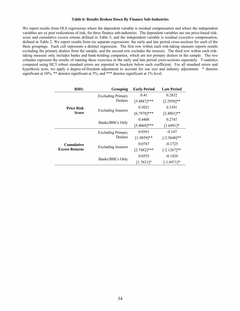
34

Table 6: Results Broken Down By Finance Sub-Industries

We report results from OLS regressions where the dependent variable is residual compensation and where the independent variables are ex post realizations of risk, for three finance sub-industries. The dependent variables are our price-based risk-score and cumulative excess returns defined in Table 5, and the independent variable is residual executive compensation, defined in Table 2. We report results from six separate regressions: the early and late period cross-sections for each of the three groupings. Each cell represents a distinct regression. The first row within each risk-taking measure reports results excluding the primary dealers from the sample, and the second row excludes the insurers. The third row within each risk-taking measure only includes banks and bank-holding companies, which are not primary dealers in the sample. The two columns represent the results of running these exercises in the early and late period cross-sections separately. T-statistics computed using HC3 robust standard errors are reported in brackets below each coefficient. For all standard errors and hypothesis tests, we apply a degree-of-freedom adjustment to account for our size and industry adjustment. * denotes significant at 10%, ** denotes significant at 5%, and *** denotes significant at 1% level.

RHS: Grouping Early Period Late Period

Price Risk Score

Excluding Primary Dealers

0.41 0.2832

[5.4887]*** [2.2958]**

Excluding Insurers 0.5021 0.3391

[6.7978]*** [2.4801]**

Banks/BHCs Only 0.4408 0.2747

[5.4069]*** [1.6991]*

Cumulative Excess Returns

Excluding Primary Dealers

0.0561 -0.147

[1.9859]** [-2.5648]**

Excluding Insurers 0.0767 -0.1725

[2.7482]*** [-2.1267]**

Banks/BHCs Only 0.0555 -0.1429

[1.7621]* [-1.6971]*

35

Table 7: Robustness Checks Each row is a different exercise and each column reports the results from an OLS regression with a different risk-taking measure as the independent variable and residual compensation as the dependent variable. Each cell represents a distinct regression. In the first row, we use residual compensation computed from book asset values instead of market capitalization as the independent variable. The second row adds a control for leverage, de-scaled by size and industry. The third row uses residual non-CEO executive compensation as the independent variable The fourth row repeats our exercise by using a sample of non-financial ExecuComp firms where we compute residual compensation along two-digit SIC codes. In the fifth row, we check whether our results are sensitive to the cutoff period by running our analysis using a pooled regression, where residual compensation is computed within each year and each measure of risk is measured using contemporaneous data on returns during that year. We then run a pooled regression of each year’s residual compensation on risk. T-statistics computed using HC3 robust standard errors are reported in brackets under each coefficient except for the last row, where we cluster standard errors by firm. For all standard errors and hypothesis tests, we apply a degree-of-freedom adjustment to account for our size and industry adjustment. * denotes significant at 10%, ** denotes significant at 5%, and *** denotes significant at 1% level.

Robustness Exercise RHS: Price Risk

Score Cumulative

Excess Return

Using book asset values when computing residual compensation

Early Period 0.45 0.0727

[4.7078]*** [2.4891]**

Late Period 0.2971 -0.2017

[2.2746]** [-3.0895]***

Controlling for book leverage and size in risk-taking regressions

Early Period 0.4511 0.07

[5.8400]*** [2.5601]**

Late Period 0.2866 -0.1548

[2.3762]** [-2.6631]***

Using only non-CEO executive compensation

Early Period 0.4365 0.0746

[6.6029]*** [2.9088]***

Late Period 0.3177 -0.1647

[2.6399]*** [-2.9093]***

Analysis on non-financial industries

Early Period 0.1532 0.0108

[6.4005]*** [1.5837]

Late Period 0.2922 -0.0026

[8.1640]*** [-0.2468]

Pooled Regression

0.4287

(1992-2008) [9.1836]***

36

Table 8: Residual Compensation, Governance, and Investors

We report results from separate OLS regressions where the dependent variables are residual compensation and our price risk score, and where the independent variables are the G Index, E Index, Percentage of Independent Directors, and Institutional Ownership, computed over 1992-1994 for the early period and 1998-2000 for the late period. Each cell represents a distinct regression. G-Index is the Gompers-Ishii-Metrick (2003) measure of managerial entrenchment. E-Index is the Bebchuk, Cohen and Ferrell (2008) measure of entrenchment. Percentage of Independent Directors is the percentage of outside directors who have no significant connection with the firm (classified as “Independent” by RiskMetrics). Institutional Ownership is defined as the total shares held by institutions reporting in 13F statements divided by the number of shares outstanding, averaged over the 12 quarters in 1992-1994 for the early period and 1998-2000 for the late period. T-statistics computed using HC3-robust standard errors are reported in brackets below each coefficient. For all standard errors and hypothesis tests, we apply a degree-of-freedom adjustment to account for our size and industry adjustment. * denotes significant at 10%, ** denotes significant at 5%, and *** denotes significant at 1% level.

LHS: Residual Compensation Price Risk Score

Early Late Early Late

RHS: Period Period Period Period

G Index 0.0053 0.0053 0.0164 0.0215

[0.3000] [0.2592] [0.7162] [0.9766]

E Index -0.0374 -0.0073 -0.0309 0.0281

[-0.6640] [-0.1575] [-0.5902] [0.5650]

% Independent Directors

0.1677 0.607

[0.3932] [1.2495]

Institutional Ownership

1.3753 1.1744 0.9983 1.0238

[4.7509]*** [4.2020]*** [2.6687]*** [3.2783]***

37

Figure 1: Log Average Executive Compensation and Market Capitalization

Panel A

Panel B

The figure plots the log of average executive compensation on the vertical axis against log market capitalization on the horizontal axis, and overlays a linear fit. Panel A plots this relationship for the early period (1992-1994) and Panel B plots this relationship for the late period (1998-2000). Slopes and intercepts are calculated using a model where all three groups (primary dealers, banks, insurers) have their own intercepts and insurers have a distinct slope from banks and primary dealers. Tickers significant to the crisis are labeled.

BACNB

BSC

CMB

CCI

TRV

MERJPMMS

CCR NOBWFC

WB

AIG

BRK

MBI

56

78

910

Log

Avg

Com

pens

atio

n, 1

992−

1994

4 6 8 101992−1994 Log Avg Market Capitalization

Primary DealersBanksInsurers

BACBSC

CMB

C

MERMWD

LEHGS

CCR WM

WFC AIG

BRK

MBI

ABK

56

78

910

11L

og A

vg C

ompe

nsat

ion,

199

8−20

00

5 7 9 11 131998−2000 Log Avg Market Capitalization

Primary DealersBanksInsurers

38

Figure 2: Residual Executive Compensation and Risk-Taking

We plot residual compensation on the vertical axis against ex post realizations of risk and outcomes on the horizontal axis for both the early and late cross-sections. Panels A and B plot the relationship of residual compensation with a firm’s price risk score. Panel C plots the relationship for Exposure to ABX, and Panels D and E plot the relationship for Cumulative Excess Returns. Each variable is adjusted for size and industry. A linear fit is overlaid and we report the slopes, t-statistics, and p-values associated with each fit. The t-statistics are calculated using HC3-robust standard errors with a degrees-of-freedom adjustment to account for our size and industry adjustment. Tickers significant to the crisis are labeled.

BACNB

BSC

CMBCCI

TRV

MERJPM

MS

CCR

NOBWFC

WB

AIG

BRK

MBI

Slope: .465t: 6.75p: 0

−2

−1

01

2R

esid

ual C

ompe

nsat

ion,

199

2−19

94

−1 −.5 0 .5 1 1.5Price Risk Score Residual, 1995−2000

Panel A

BAC

BSC

CMBC

MERMWD

LEH

GSCCR

WMWFC

AIG

BRK

MBI

ABK

Slope: .328t: 2.96p: .004

−2

−1

01

2R

esid

ual C

ompe

nsat

ion,

199

8−20

00

−1 0 1 2Price Risk Score Residual, 2001−2008

Panel B

BAC

BSC

CMBC

MERMWD

LEH

GS

CCR

WMWFC

AIG

BRK

MBI

ABK

Slope: .827t: 2.76p: .007

−2

−1

01

2R

esid

ual C

ompe

nsat

ion,

199

8−20

00

−1 −.5 0 .5 1Exposure to ABX Residual, 2006−2008

Panel C

BACNB

BSC

CMBCCI

TRV

MERJPM

MS

CCR

NOBWFC

WB

AIG

BRK

MBI

Slope: .074t: 2.90p: .004

−2

−1

01

2R

esid

ual C

ompe

nsat

ion,

199

2−19

94

−4 −2 0 2 4 6Excess Return Residual, 1995−2000

Panel D

BAC

BSC

CMBC

MERMWD

LEH

GSCCR

WM WFC

AIG

BRK

MBI

ABK

Slope: −.16t: −2.9p: .004

−2

−1

01

2R

esid

ual C

ompe

nsat

ion,

199

8−20

00

−2 −1 0 1 2 3Excess Return Residual, 2001−2008

Panel E

39

Appendix: Proofs

Proposition. Suppose the disutility of effort satisfies > 0, > 0, and < 2 for a > 0. If = 0, then > 0 and > 0.

Proof. If = 0 then direct computation shows that

ℎ = ℎ ′′2 − ′

By supposition, , > 0, so the sign of is determined by the sign of 2 − . For cost

functions such that < 2 , we have that > 0 is then a necessary condition for = 0. From

the equilibrium condition ( ) = ℎ, direct computation shows that

= 1′′ ℎ + ℎ = ℎ > 0

Direct computation also shows that = ( ) + > 0. Note that the condition on the cost

function c is satisfied by every = for > 1, > 0 and also every exponential function of the

form = exp( ) with > 0. Notice that a > 0 in equilibrium so we do not have to worry about the

denominator going to zero.

More generally, we have

ℎ = −1 1 + ℎ − ℎ ′′ ℎ − ′′ℎ− ℎ 2 − ′

If ≥ 0, with the additional assumption that > 0, then > 0. Since = +ℎ > 0 and

= ( ) + + 2 > 0

the conclusion follows. ■