NBER WORKING PAPER SERIES

MATERNAL HEALTH AND THE BABY BOOM

Stefania AlbanesiClaudia Olivetti

Working Paper 16146http://www.nber.org/papers/w16146

NATIONAL BUREAU OF ECONOMIC RESEARCH1050 Massachusetts Avenue

Cambridge, MA 02138July 2010

We thank Jerome Adda, Joshua Aizenman, Andy Atkeson, Hoyt Bleakley, Miriam Bruhn, FranciscoBuera, Jesus Fernandez-Villaverde, Claudia Goldin, Jeremy Greenwood, Michael Haines, ChristianHellwig, Sok Chul Hong, Andrea Ichino, Nir Jaimovich, Larry Katz, Dirk Krueger, Adriana Lleras-Muney,David Lyle, Lee Ohanian, Nicola Pavoni, Valerie Ramey, Garey Ramey, Fabiano Schivardi, RobertTamura, Michele Tertilt, Guillaume Vanderbroucke, and seminar participants at UCLA, UCSC, UCSD,Stanford, the NBER Macroeconomics Across Time and Space and Development of the AmericanEconomy Groups, the NY-Philadelphia Quantitative Macroeconomics Workshop, Columbia University,Georgetown University, UCL, Universita' Federico II, the Bank of Italy and the European UniversityInstitute for helpful comments and suggestions. We are grateful to Maria J. Prados for outstandingresearch assistance and Junya Khan-Lang and Vighnesh Subramanyan who contributed to data collection.This work is supported by the National Science Foundation under Grant SES 0820135. Stefania Albanesigratefully acknowledges financial support and hospitality from the Hoover Institution and EIEF whileworking on this project. The views expressed herein are those of the authors and do not necessarilyreflect the views of the National Bureau of Economic Research.

NBER working papers are circulated for discussion and comment purposes. They have not been peer-reviewed or been subject to the review by the NBER Board of Directors that accompanies officialNBER publications.

© 2010 by Stefania Albanesi and Claudia Olivetti. All rights reserved. Short sections of text, not toexceed two paragraphs, may be quoted without explicit permission provided that full credit, including© notice, is given to the source.

Maternal Health and the Baby BoomStefania Albanesi and Claudia OlivettiNBER Working Paper No. 16146July 2010JEL No. J11,J13,J24,N12,N3,N92

ABSTRACT

U.S. fertility rose from a low of 2.27 children for women born in 1908 to a peak of 3.21 children forwomen born in 1932. It dropped to a new low of 1.74 children for women born in 1949, before stabilizingfor subsequent cohorts. We propose a novel explanation for this boom-bust pattern, linking it to thehuge improvements in maternal health that started in the mid 1930s. Our hypothesis is that the improvementsin maternal health contributed to the mid-twentieth century baby boom and generated a rise in women'shuman capital, ultimately leading to a decline in desired fertility for subsequent cohorts. To examinethis link empirically, we exploit the large cross-state variation in the magnitude of the decline in pregnancy-related mortality and the differential exposure by cohort. We find that the decline in maternal mortalityis associated with a rise in fertility for women born between 1921 and 1940, with a rise in collegeand high school graduation rates for women born in 1933-1950, and with a decline in fertility for womenborn in 1941-1950. These findings are consistent with a theory of fertility featuring a trade-off betweenthe quality and quantity of children. The analysis provides new insights on the determinants of fertilityin the U.S. and other countries that experienced similar improvements in maternal health.

Stefania AlbanesiColumbia University1022 International Affairs Building420 West 118th StreetNew York, NY 10027and NBERstefania.albanesi@columbia.edu

Claudia OlivettiNational Bureau of Economic Research1050 Massachusetts AvenueCambridge, MA 02138and NBERolivetti@bu.edu

Contents

1 Introduction 2

2 Maternal Health in the US 52.1 Burden of Maternal Mortality and Morbidity . . . . . . . . . . . . . . . . . . . . . . . . . . . 52.2 Advances in Maternal Health . . . . . . . . . . . . . . . . . . . . . . . . . . . . . . . . . . . . 52.3 Historical Background . . . . . . . . . . . . . . . . . . . . . . . . . . . . . . . . . . . . . . . . 7

3 Theory 10

4 Empirical Analysis 144.1 Fertility . . . . . . . . . . . . . . . . . . . . . . . . . . . . . . . . . . . . . . . . . . . . . . . . 16

4.1.1 Baseline Results . . . . . . . . . . . . . . . . . . . . . . . . . . . . . . . . . . . . . . . 174.1.2 Sensitivity . . . . . . . . . . . . . . . . . . . . . . . . . . . . . . . . . . . . . . . . . . . 204.1.3 Marriage Rates and Childlessness . . . . . . . . . . . . . . . . . . . . . . . . . . . . . . 244.1.4 Fertility by Education . . . . . . . . . . . . . . . . . . . . . . . . . . . . . . . . . . . . 27

4.2 Education . . . . . . . . . . . . . . . . . . . . . . . . . . . . . . . . . . . . . . . . . . . . . . . 294.2.1 Baseline Results . . . . . . . . . . . . . . . . . . . . . . . . . . . . . . . . . . . . . . . 314.2.2 Sensitivity . . . . . . . . . . . . . . . . . . . . . . . . . . . . . . . . . . . . . . . . . . . 31

4.3 Baby Bust . . . . . . . . . . . . . . . . . . . . . . . . . . . . . . . . . . . . . . . . . . . . . . . 35

5 Concluding Remarks 39

A Data Sources and Variable Definitions 44A.1 Fertility and Education Data . . . . . . . . . . . . . . . . . . . . . . . . . . . . . . . . . . . . 44A.2 Mortality Data . . . . . . . . . . . . . . . . . . . . . . . . . . . . . . . . . . . . . . . . . . . . 45A.3 State Level Controls . . . . . . . . . . . . . . . . . . . . . . . . . . . . . . . . . . . . . . . . . 46

B Government Intervention in the Area of Maternal Health 47

C Theory 49C.1 Basic Model . . . . . . . . . . . . . . . . . . . . . . . . . . . . . . . . . . . . . . . . . . . . . . 49

C.1.1 Proofs . . . . . . . . . . . . . . . . . . . . . . . . . . . . . . . . . . . . . . . . . . . . . 49C.1.2 Response to a Temporary Decline in Maternal Mortality . . . . . . . . . . . . . . . . . 50

C.2 Extended Model . . . . . . . . . . . . . . . . . . . . . . . . . . . . . . . . . . . . . . . . . . . 51

D Additional Empirical Results 54

1

1 Introduction

The United States experienced very big swings in fertility between the late 1930s and the early 1970s. Thecohort total fertility rate1 rose from a low of 2.27 children for women born in 1908 to a peak of 3.21 childrenfor women born in 1932. After dropping to a new historical low of 1.74 children for women born in 1949,the rate stabilized at around 2 children per woman in the 1980s. Despite the remarkable magnitude of thesefluctuations in fertility and their clear economic and social relevance, their origins are still poorly understood.Perhaps the best known theory is Easterlin’s (1961) “relative income” hypothesis, based on the notion thatparticularly favorable labor market conditions tend to increase desired fertility. Thus, the recovery fromthe Great Depression and World War II can provide an explanation for the baby boom. This hypothesis,however, runs counter to the very strong negative empirical correlation between income and fertility (Jonesand Tertilt, 2007).

We propose a novel explanation for the boom and bust in U.S. fertility that links these phenomena to thedramatic improvements in maternal health that occurred starting in the mid-1930s. In 1900, one mother diedfor every 118 live births, and pregnancy related causes accounted for over 15% of all deaths of women 15-44between 1900 and 1930, the second largest cause of death after tuberculosis. In 1936, maternal mortalitystarted to fall sharply, reaching modern levels by the late 1950s. Pregnancy related deaths dropped from 1for every 195 live births in 1936 to 1 for every 3,484 live births in 1956. The virtual elimination of maternalmortality risk was accompanied by a similar reduction in the incidence of pregnancy-related conditions, andby a rise in the female-male di!erential in adult life expectancy from 2.5 to 6 years over the same period.

Our hypothesis is that the improvement in maternal health contributed to the mid-twentieth century babyboom and generated a rise in women’s human capital, ultimately leading to a decline in desired fertility forsubsequent cohorts. We formalize this reasoning with a stylized model of fertility choice and costly parentalhuman capital investment, which incorporates pregnancy-related death risk and a quality/quantity trade-o!in the demand for children, as in Becker and Barro (1988). The model predicts that both fertility and parentalinvestments in daughters’ human capital will rise in response to a permanent decline in pregnancy-relatedmortality, as the health cost of childbearing declines and women’s productive life span expands. While therise in women’s human capital is permanent, the increase in fertility is only temporary. Given that womenwho experienced the decline in maternal mortality in their formative years have higher education and higheropportunity cost of children, they will have lower desired fertility than older women who experienced thedecline having completed their education. The resulting boom-bust pattern in fertility qualitatively replicatesthe U.S. experience. Since the e!ects on women’s human capital are permanent, the long run e!ect on fertilitymay well be negative, if the returns to human capital are high enough.

Our empirical strategy exploits the large cross-state variation in the magnitude of the maternal mortalitydecline to estimate the e!ect of the decline on the change in completed fertility and educational attainmentacross cohorts of women who were di!erentially exposed. The year 1936 marks the start of the rapid declinein maternal mortality for the U.S., and we use this date to identify the treated cohorts. Panel estimatessuggest that for every standard deviation reduction in maternal mortality, completed fertility rises by 0.41

1The Cohort Total Fertility Rate (CTFR) is a measure of the total lifetime fertility of the average woman born in a givenyear. Formally, let fa,t be the number of children born to women of age a in period t divided by the number of those women.Then, CTFRt =

Pa=49a=15 fa,t+a. This measure is preferable to the more often used Period Total Fertility Rate (PTFR), defined

as PTFRt =Pa=49

a=15 fa,t, in time periods when total fertility changes across cohorts since it does not mix fertility behavior ofdi!erent cohorts. The CTFR is shifted by 27 years to align its peak to the the PTFR. The CTFR underestimates completedfertility if maternal death risk is high. Both series are plotted in figure 1. See Jones and Tertilt (2007) for a discussion ofalternative fertility measures.

2

!"!!#

$!"!!#

%!"!!#

&!"!!#

'!"!!#

(!"!!#

)!"!!#

*!"!!#

+!"!!#

,!"!!#

$!!"!!#

$"*!#

%"%!#

%"*!#

&"%!#

&"*!#

'"%!#

$,!!#

$,!(#

$,$!#

$,$(#

$,%!#

$,%(#

$,&!#

$,&(#

$,'!#

$,'(#

$,(!#

$,((#

$,)!#

$,)(#

$,*!#

$,*(#

$,+!#

$,+(#

-./012#345#67809.:;# <345=%*# >?9./@?A#>1/9?A09B#/?9.##

6C./#$!D!!!#A0E.#F0/98:;#

Figure 1: Maternal mortality, Period Total Fertility Rate and Cohort Total Fertility Rate (+27) in the U.S. 1900-1990Source: U.S. Cohort Fertility Tables, CTFR 1917-1980, TFR 1900-1988. Produced by the National Institute of Child Health, compiled

in Heuser (1976). U.S. Period Fertility Rate in Haines (2006). Maternal mortality from Vital Statistics of the United States.

children for women born in 1921-1940 relative to a control group of those born in 1913-1920, about 29%of the actual rise. The di!erential decline in maternal mortality accounts for over 45% of the cross-statevariation in the change in fertility between cohorts.

The estimates suggest that the maternal mortality decline also had a very strong e!ect on the growth inwomen’s educational attainment relative to men. For every standard deviation drop in maternal mortality,the female-male di!erential in graduation rates rises by 0.017 for college and by 0.046 for high school forthe 1933-1950 birth cohorts. This accounts for 40% and 56%, respectively, of the actual rise relative to thecontrol group. These findings are robust to the inclusion of economic and demographic controls, includingearly access to oral contraception for the treated cohorts.

Finally, we examine whether the decline in maternal mortality contributed to the decline in fertility thatoccurred between the early 1960s and the mid 1970s. We compare fertility outcomes of cohorts of womenborn in 1941-1950 whose education rose in response to the decline in maternal mortality, to outcomes ofwomen who had completed their education when maternal mortality started to decline and only respondedwith fertility. Our estimates suggest that the the decline in maternal mortality played a significant role in thebaby bust. A standard deviation reduction in maternal mortality is associated with a decline in completedfertility by 0.47 children, or 77% of the actual decline across these groups of cohorts. Our estimates arerobust to the inclusion of controls for early access to oral contraception.

These results suggest that the decline in maternal mortality contributed significantly to the US babyboom and subsequent baby bust, providing a novel, integrated explanation for these important demographicphenomena. Moreover, we show that the decline in pregnancy-related mortality had a sizable impact on therise in the female-male di!erential in college graduation. This trend, which began with individuals born inthe mid 1930s (Goldin, Katz and Kuziemko, 2007), has been explained mainly in terms of the introductionoral contraception (Goldin and Katz, 2002, and Bailey, 2006). We interpret the rapid adoption of oral

3

contraception by young women in the late 1960s as spurred by a desire to reduce and postpone fertility,which originated at least in part from the improvement in maternal health and its e!ect on the returns tohuman capital investment.

This paper’s main contribution is to the macroeconomic literature on the baby boom. Greenwood,Seshadri and Vanderbroucke (2005) propose that the di!usion of home appliances was a key determinantof the baby boom, as it reduced the time cost of children. This explanation is not fully consistent withthe timing of the baby boom, as fertility started to rise prior to World War II, while the di!usion of homeappliances took o! in the 1950s and 1960s2. It also leaves open the possibility that the rise in fertility andthe resulting increase in the number of children per household, a key determinant of the demand for homehours (Ramey, 2008), may have increased the demand for home appliances3.

Doepke, Hazan and Maoz (2007) argue that World War II was an important factor for the baby boom.The rise in labor force participation of married women during the war crowded out younger women after thewar, causing them to opt for marriage and childbearing. This explanation is inconsistent with the fact thatfertility began to rise before the war and with the limited direct impact of wartime female participation onlabor market conditions. According to Goldin (1991), of the 80% of women who were not working in 1941,14% were working in 1944 and only 46% of these were still in the labor force in 1951.4 Moreover, Acemoglu,Autor and Lyle (2004) find that the impact of wartime female participation on wages was largely exhaustedby 1950. Finally, this hypothesis is based on the premise that women who became mothers during the babyboom were not in the workforce, while Albanesi and Olivetti (2009) show that participation of mothers roseduring the baby boom.

The paper also contributes to the literature on the e!ect of disease eradication on human capital. Themost closely related paper in this area is Jayachandran and Lleras-Muney (2009), who study of the impactof maternal mortality decline on female literacy in Sri Lanka.5 Their estimates suggest a strong positivee!ect, which they interpret as consistent with a rise in parental investments in the education of daughters.Our results confirm the strong impact of falling maternal mortality on women’s education for the U.S. Ouranalysis di!ers though, since our main goal is to trace out the joint response of both fertility and women’shuman capital for successive generations of women, not only the short run response in girls’ education.

Finally, we suggest a new mechanism through which mortality reductions can influence fertility. Followingthe pioneering work of Preston (1978), the demographic literature has concentrated on the impact of thereduction in youth mortality on the secular decline in fertility (Preston and Haines, 1991, and Haines, 1997)6.We show that a decline in maternal mortality induces a temporary rise in fertility, which points to medicalprogress as an integrated explanation for both the secular trend and the medium run fluctuations in fertility.

Our findings provide new insights on the determinants of fertility in the United States and other countriesthat experienced similar advances in maternal health, and o!er a new perspective on demographic policies indeveloping countries. Albanesi and Olivetti (2009) show that improved maternal health was critical for therise in labor force participation of married women during the twentieth century, generating a rise in incomeper capita of over 50% via this channel. These results suggest that improving maternal health, typically avery severe problem in developing countries, could improve standards of living substantially even without a

2See Albanesi (2008) for a discussion.3Bailey and Collins (2009) find that di!erences and changes in appliance ownership and electrification in U.S. counties are

negatively correlated with fertility rates from 1940 to 1960.4Table 19, Goldin (1991).5Bleakley (2007) and Bleakley and Lange (2008) study the impact of malaria and hookworm eradication on fertility and

schooling in the American South. They find a negative e!ect on fertility and a sizable positive e!ect on schooling.6Doepke (2005) provides an excellent discussion.

4

decline in fertility.The paper is organized as follows. Section 2 discusses the historical background for the reduction in

maternal mortality in the U.S. Section 3 presents a model of fertility choice with human capital investmentto examine the impact of a decline in maternal mortality. Section 4 discusses the empirical analysis. Section4.1 concentrates on the fertility response of women who had completed their education at the onset of thedecline in maternal mortality. Section 4.2 is devoted to the response of female-male di!erentials in educationalattainment for individuals in their formative years at the time of the decline. Section 4.3 examines the linkbetween the baby bust and the decline in maternal mortality. Finally, Section 5 concludes.

2 Maternal Health in the US

This section documents the incidence of pregnancy related deaths in the early years of the twentieth century,and discusses the main developments leading to the remarkable improvements in maternal health that beganin the mid 1930s.

2.1 Burden of Maternal Mortality and Morbidity

The maternal mortality rate (MMR),7 which can be interpreted as a measure of the average probability ofa maternal death for each live birth, was equal in 1900 to 85 maternal deaths per 10,000 live births, or justunder 1%. Maternal deaths accounted for 3.2% of all female deaths and for 14.9% of all female deaths atage 15-44 in 1900, as shown in Table 1. Maternal mortality declined by only 4.5% between 1900 and 1930,whereas mortality for all causes declined by 37% for females and 32% for males. Mortality for tuberculosisdropped by over 60% in this period. The decline of maternal deaths as a fraction of all female deaths from3.1% to 1.6% between 1900 and 1930 is mostly accounted for by the decline in births in this period.8 In1930, maternal mortality still accounted for 10.6% of female deaths at age 15-44 and was the second biggestcause of death for women in this age group after tuberculosis.9

2.2 Advances in Maternal Health

The systematic decline in maternal mortality did not start until 1936 but was precipitous in the two sub-sequent decades. The maternal mortality rate dropped from 51.16 per 10,000 live births in 1936 to to 2.87in 1956, a 94% drop over a span of just twenty years. This corresponds to a -13.23% average yearly change

7According to the World Health Organization, a maternal death is the death of a woman while pregnant or within 42 daysof termination of pregnancy, irrespective of the duration and the site of the pregnancy, from any cause related to or aggravatedby the pregnancy or from its management, but not from accidental and incidental causes. Maternal deaths are divided into twogroups: Direct obstetric deaths, which result from obstetric complications of the pregnant state, or from omissions, interventions,or incorrect treatment of that state; Indirect obstetric deaths, which result from previous existing diseases that were aggravatedby the pregnancy. This distinction was not made for early maternal mortality data, thus the statistics we use throughout thepaper count both direct and indirect obstetric deaths.

8The pregnancy-related mortality risk depends on age and parity. The maternal death rate has a U-shaped relation withboth age and parity (Berry, 1977). The parity adjustment factors over average maternal mortality risk are 1.14, 0.62, 0.64,0.77, 0.99, 1.12, 1.14, 1.58 for parities 1 to 8, respectively. Dublin (1936) estimates that the parity and age distribution wasparticularly favorable for the 1905-1915 birth cohorts relative to earlier cohorts, due to their low fertility, which can accountfor most of the reduction in maternal mortality between 1900 and 1930. Changes in the age and parity distribution between1936 and the mid 1950s do not influence the pregnancy-related mortality risk.

9Maternal mortality exhibits a large spike during the 1918-1919 influenza epidemic, which also causes a temporary decline inthe male-female mortality rate and the female-male di!erential in life expectancy at age 20 between 1915 and 1920. Noymer andGarenne (2000) show that this drop resulted from the e!ects of the influenza epidemic on female-male mortality di!erentials fortuberculosis. Influenza increased mortality associated with tuberculosis. Though in general tuberculosis mortality rates werehigher for men, they increased for women during the influenza outbreak of 1918, temporarily closing the gender gap.

5

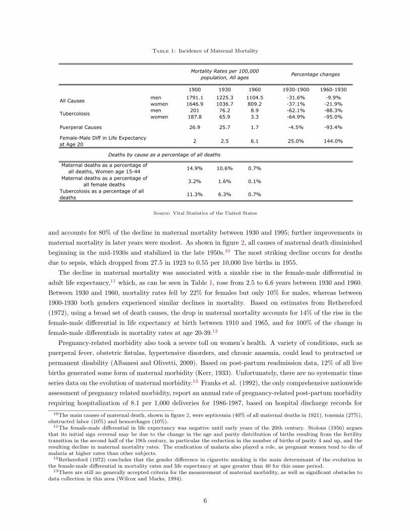
Table 1: Incidence of Maternal Mortality

1900 1930 1960 1930-1900 1960-1930

men 1791.1 1225.3 1104.5 -31.6% -9.9%women 1646.9 1036.7 809.2 -37.1% -21.9%men 201 76.2 8.9 -62.1% -88.3%women 187.8 65.9 3.3 -64.9% -95.0%

Puerperal Causes 26.9 25.7 1.7 -4.5% -93.4%

Female-Male Diff in Life Expectancy at Age 20

2 2.5 6.1 25.0% 144.0%

Maternal deaths as a percentage of all deaths, Women age 15-44

14.9% 10.6% 0.7%

Maternal deaths as a percentage of all female deaths

3.2% 1.6% 0.1%

Tubercolosis as a percentage of all deaths

11.3% 6.3% 0.7%

Deaths by cause as a percentage of all deaths

Incidence of Maternal Mortality

Mortality Rates per 100,000 population, All ages

Percentage changes

All Causes

Tubercolosis

Source: Vital Statistics of the United States

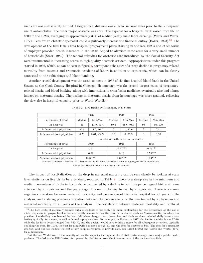
and accounts for 80% of the decline in maternal mortality between 1930 and 1995; further improvements inmaternal mortality in later years were modest. As shown in figure 2, all causes of maternal death diminishedbeginning in the mid-1930s and stabilized in the late 1950s.10 The most striking decline occurs for deathsdue to sepsis, which dropped from 27.5 in 1923 to 0.55 per 10,000 live births in 1955.

The decline in maternal mortality was associated with a sizable rise in the female-male di!erential inadult life expectancy,11 which, as can be seen in Table 1, rose from 2.5 to 6.6 years between 1930 and 1960.Between 1930 and 1960, mortality rates fell by 22% for females but only 10% for males, whereas between1900-1930 both genders experienced similar declines in mortality. Based on estimates from Rethereford(1972), using a broad set of death causes, the drop in maternal mortality accounts for 14% of the rise in thefemale-male di!erential in life expectancy at birth between 1910 and 1965, and for 100% of the change infemale-male di!erentials in mortality rates at age 20-39.12

Pregnancy-related morbidity also took a severe toll on women’s health. A variety of conditions, such aspuerperal fever, obstetric fistulas, hypertensive disorders, and chronic anaemia, could lead to protracted orpermanent disability (Albanesi and Olivetti, 2009). Based on post-partum readmission data, 12% of all livebirths generated some form of maternal morbidity (Kerr, 1933). Unfortunately, there are no systematic timeseries data on the evolution of maternal morbidity.13 Franks et al. (1992), the only comprehensive nationwideassessment of pregnancy related morbidity, report an annual rate of pregnancy-related post-partum morbidityrequiring hospitalization of 8.1 per 1,000 deliveries for 1986-1987, based on hospital discharge records for

10The main causes of maternal death, shown in figure 2, were septicemia (40% of all maternal deaths in 1921), toxemia (27%),obstructed labor (10%) and hemorrhages (10%).

11The female-male di!erential in life expectancy was negative until early years of the 20th century. Stolons (1956) arguesthat its initial sign reversal may be due to the change in the age and parity distribution of births resulting from the fertilitytransition in the second half of the 19th century, in particular the reduction in the number of births of parity 4 and up, and theresulting decline in maternal mortality rates. The eradication of malaria also played a role, as pregnant women tend to die ofmalaria at higher rates than other subjects.

12Rethereford (1972) concludes that the gender di!erence in cigarette smoking is the main determinant of the evolution inthe female-male di!erential in mortality rates and life expectancy at ages greater than 40 for this same period.

13There are still no generally accepted criteria for the measurement of maternal morbidity, as well as significant obstacles todata collection in this area (Wilcox and Marks, 1994).

6

!"#$%&' ()*+)",,-#.&/%", $/ 0"1)*#2%3$." !"#$%$/"

0.0

50.0

100.0

150.0

200.0

250.0

300.0

1921

1924

1927

1930

1933

1936

1939

1942

1945

1948

1951

1954

1957

1960

1963

1966

1969

1972

1975

1978

1981

1984

1987

1990

1993

1996

Year

Rat

es p

er 1

00

,00

0 l

ive

bir

ths

Toxemias

Hemorrhage

Sepsis

Traumatic Accidents of Labor

4$+2)"5 6)"/#, $/ %&2,", *7 8&3")/&' #"&39,Figure 2: Maternal mortality by cause

Source: Vital Statistics of the United States

the United States. The corresponding statistic for the late 1920s reported in Kerr (1933) is 114.4 per1,000 deliveries.14 Thus, post-partum pregnancy-related conditions requiring hospitalization dropped by93% between the late 1920s and the mid 1980s, a magnitude similar to the drop in maternal mortality overthe same period (1930-1987). On this basis, the analysis will maintain the assumption that the decline inmaternal mortality is accompanied by a similar reduction in pregnancy-related morbidity. This assumptionis standard in the literature on the economic impact of disease eradication.15

2.3 Historical Background

Women were keenly conscious of the health risks associated with pregnancy and childbirth, yet it wasn’tuntil the 1920s that maternal mortality started to be considered a major health problem in the U.S. (Leavitt,1986).

Early e!orts to improve maternal health were driven mainly by the goal of reducing infant mortality,which was very high, especially in urban areas (Meckel, 1990). The Children’s Bureau, created by an act ofCongress in 1912, was the first federal agency with the primary responsibility of promoting infant and childhealth16. One of its main activities was to conduct detailed statistical studies of maternal and child healthoutcomes.

In 1917, the Children’s Bureau submitted a report to Congress on “Maternal Mortality from All Con-ditions Connected with Childbirth in the United States and Certain Other Countries” (Meigs, 1917). Themain findings were that maternal mortality was the second largest cause of death for women age 15-44 after

14This statistic is based on 1.0646 deliveries per live birth in 1930, using the infant mortality rate for that year, and thematernal mortality rate in 1930, equal to 60.90 maternal deaths per 10,000 live births.

15Weil (2004) o!ers an excellent discussion of this approach.16For a detailed account of the establishment of the Children’s Bureau, see Schmidt (1973), Parker and Carpenter (1981) and

Skopcol (1992). The Children’s Bureau was modelled on New York City’s Department of Child Hygiene, the first of its kind,founded in 1908. For a full account see: http://www.ssa.gov/history/childb1.html

7

tuberculosis in 1913, and that the United States was the worst for maternal health among advanced nations.Following this report, the Children’s Bureau became the main sponsor and administrator of a series of keyfederal programs, explicitly targeting maternal and infant health, introduced between 1921 and 1943. Themost notable were the Sheppard-Towner Act of 1921-1929, which provided federal funding to the statesfor educational activities for the promotion of maternal and infant health, and the Social Security Act of1935. Title V, Part 1 of this act provided federal funding to the states on a grant-in-aid basis for directsubsidies for obstetric and infant care. Finally, the Emergency Infant and Maternal Care program providedfull coverage for obstetric and infant care for the wives and children of servicemen between 1941 and 1946.A brief description of the these programs, including the criteria for appropriation, is provided in AppendixB.

The Children’s Bureau was also instrumental in raising awareness of the preventability of pregnancy-related mortality in the medical profession. While physicians systematically started to enter the birth roomin 1850, their intervention did not contribute initially to a reduction in maternal mortality.17 Inappropriateand excessive operative procedures were common and increased in the 1920s, leading to high rates of birthinjuries for both newborns and mothers (Loudon, 1992).

The iatrogenic nature of obstetric complications and pregnancy related mortality in the early phasesof the medicalization of childbirth received widespread public attention following the publication of theproceedings from the 1930 White House Conference on Child Health and Protection, sponsored by theChildren’s Bureau.18 More than two-thirds of all maternal deaths were found to be preventable for anationally representative sample, and many physicians were found to lack the most basic obstetric knowledge(CDC, 1999). 19

These reports precipitated e!orts to standardize obstetric practices and train physicians. Alongsidea number of scientific discoveries and advances in general medicine that took place in the 1930s, thesedevelopments led to a fast decline in maternal mortality.

As can be seen from figures 1 and 2, the year 1936 brought a clear break in pregnancy related mortality.In 1936, sulphonamides, the first type of antibiotic, were introduced. These drugs were relatively cheap toproduce and di!used very rapidly, bringing down mortality for several diseases, such as pneumonia, influenza,and scarlet fever, in a span of just a few years (Jayachandran, Lleras-Muney and Smith, 2009). Given thatpuerperal sepsis accounted for approximately 40% of all maternal deaths in 1936, the introduction of sulfadrugs had a very large impact on maternal mortality. Later, the discovery of the antibiotic e!ects of penicillin(1939-1942) also contributed to the decline in maternal mortality due to sepsis.

There was also a widespread improvement in obstetric care in hospitals, following the establishment of theAmerican Board of Obstetrics and Gynecology in 1930 (Dannreuther, 1931). Residency training programswere set up in the 1930s to prevent hospitals from accepting unqualified specialists. Hospital and statematernal mortality review committees also were established in the 1930s and 1940s.

Even as the quality of obstetric care was improving in many hospitals starting in the 1930s, access to17Thomasson and Treber (2008) analyze the consequences of the hospitalization of childbirth on maternal mortality in the

US.18Convened in 1930 by President Herbert Hoover, the White House Conference on Child Health and Protection was called

"to study the present status of the health and well-being of the children of the United States and its possessions, to reportwhat was being done, to recommend what ought to be done and how to do it." The resulting “Child Health Protection, FetalNewborn, and Maternal Mortality and Morbidity Report,” published in 1933, and the committee reports laid the groundworkfor the Fair Labor Standard Act of 1938 and for inclusion in the Social Security Act of 1935 of the federal-state programs foraid to dependent children, crippled children, and maternal and child-health/welfare services.

19Similar findings emerged from a study of 2,041 maternal deaths in childbirth by the New York Academy of Medicine,published in 1933.

8

such care was still severely limited. Geographical distance was a factor in rural areas prior to the widespreaduse of automobiles. The other major obstacle was cost. The expense for a hospital birth varied from $50 to$300 in the 1920s, averaging to approximately 30% of median yearly male labor earnings (Wertz and Wertz,1977). Fees for an obstetric specialist could significantly increase the financial outlay (Baker, 1923).20 Thedevelopment of the first Blue Cross hospital pre-payment plans starting in the late 1920s and other formsof employer provided health insurance in the 1930s helped to alleviate these costs for a very small numberof households (Starr, 1982). The federal subsidies for obstetric care introduced by the Social Security Actwere instrumental in increasing access to high quality obstetric services. Appropriations under this programstarted in 1936, which, as can be seen in figure 2, corresponds the start of a steep decline in pregnancy-relatedmortality from toxemia and traumatic accidents of labor, in addition to septicemia, which can be clearlyconnected to the sulfa drugs and blood banking.

Another crucial development was the establishment in 1937 of the first hospital blood bank in the UnitedStates, at the Cook County Hospital in Chicago. Hemorrhage was the second largest cause of pregnancy-related death, and blood banking, along with innovations in transfusion medicine, eventually also had a largeimpact on maternal deaths. The decline in maternal deaths from hemorrhage was more gradual, reflectingthe slow rise in hospital capacity prior to World War II.21

Table 2: Live Births by Attendant, U.S. States

1940 1946 1954

Percentage of total Median Min,Max Median Min,Max Median Min,Max

In hospital 61 13.9, 91.4 89.6 38.6, 98.9 98 60, 100

At home with physician 36.6 8.6, 76.7 9 1, 42.6 2 0,11

At home without physician 0.71 0.01, 49.29 0.6 0, 36.9 0 0,30

Correlation with maternal mortality

Percentage of total 1940 1946 1954

In hospital -0.31 -0.42*** -0.73***

At home with physician 0.09 0.16 0.59***

At home without physician 0.47*** 0.68*** 0.74***Source: Children’s Bureau. *** Significant at 1% level. Statistics refer to aggregate state population.

Alaska and Hawaii are excluded from the sample.

The impact of hospitalization on the drop in maternal mortality can be seen clearly by looking at statelevel statistics on live births by attendant, reported in Table 2. There is a sharp rise in the minimum andmedian percentage of births in hospitals, accompanied by a decline in both the percentage of births at homeattended by a physician and the percentage of home births unattended by a physician. There is a strongnegative correlation between maternal mortality and percentage of births in hospital for all years in theanalysis, and a strong positive correlation between the percentage of births unattended by a physician andmaternal mortality for all years of the analysis. The correlation between maternal mortality and births at

20The high costs of medically trained birth attendants is probably the main explanation for the persistence of the use ofmidwives, even in geographical areas with easily accessible hospital care or in states, such as Massachusetts, in which thepractice of midwifery was banned by law. Midwives charged much lower fees and their services included daily home visits,lasting typically for a week, as well as housekeeping services. For example, in Detroit in 1917, the fee for a midwife was $7-10,while the fee for a doctor ranged from $20-30, and the patient would have to hire a nurse for all subsequent attention, typicallydoubling the cost. By 1930, the cost for a midwife had risen to $25-30, and the cost for doctors to $65. The cost for a specialistwas $75, and did not include the cost of any supplies required to provide care. See Lito! (1986) and Wertz and Wertz (1977)for a discussion.

21At the end World War II, the scarcity of hospital capacity throughout the United States emerged as a major public healthproblem. This led to the Hill-Burton Act, passed in 1946 to improve the infrastructure of the nation’s hospitals.

9

home attended by a physician is also positive for all years, but it becomes sizable and significant at the 1%level only for 1954.

3 Theory

We now examine a version of Becker and Barro’s (1988) model of fertility choice that explicitly incorporatesmaternal mortality. The model predicts that a decline in maternal mortality is associated to a temporaryrise in fertility and a permanent rise in women’s human capital. These predictions will provide a conceptualframework for the empirical analysis.

We begin to illustrate the e!ect of pregnancy-related mortality risk on fertility choice and human capitalinvestment in a simple model inhabited only by women, that is, all adults are female and all o!spring arefemale. This framework, though clearly not realistic, captures the essential forces shaping fertility decisions,and the incentives to invest in daughters’ human capital. Appendix C.2 analyzes a general version of themodel, which features individuals and o!spring of both genders, delivering the same results.

Women derive utility from consumption and from the quantity and quality of their children. The lattersimply corresponds to the children’s endowment of human capital, which can be raised via a costly maternalinvestment and raises the children’s lifetime utility. Mothers may die in childbirth. Their mortality risk is afunction of the pregnancy-related mortality rate, which they take as given, and of the number of births.

The women’s decision problem is captured by the following Bellman equation:

U(e; !) = maxe!!0,b!0 {"v(b, e") + (1" µb)u(w(1 + "e)) + #$(sb)U(e"; !")} ,

where e # 0 represents mother’s human capital and e" is a mother’s investment in the daughters’ humancapital, b is the number of births.

The function v(·) represents the utility cost of parental investment in children’s human capital, whichdepends on the number of children. The function v(·) is strictly increasing in both arguments and convex.

The parameter µ $ [0, 1] corresponds to the pregnancy-related mortality probability associated with eachbirth, and (1 " µb) is the probability that a woman will survive childbearing. The function u(·) is theutility from mothers’ consumption, which depends on baseline income, w, and their endowment of humancapital e. The parameter " # 0 is the return to human capital investment. Mothers with higher humancapital enjoy higher utility from consumption if they survive childbirth. We assume u(·) is twice continuouslydi!erentiable, with u(·) > 0, u"(·) > 0 and u""(·) % 0.

The parameter s $ (0, 1] denotes the youth survival probability, thus, sb is the number of childrensurviving to adulthood. The function $(·) corresponds to the Barro-Becker dynastic discount factor for theutility from children, with $(·) $ [0, 1) $"(·) > 0 and $""(·) % 0 and limx#0$"(x) = +&. The functions v(·) ,u(·) and $(·), are twice continuously di!erentiable.

The function U(e;µ) is the value function for a cohort’s problem, and can be interpreted to correspond tothe “quality” of a given cohort. We index this value function by the pregnancy-related mortality risk, whichis allowed to vary across cohorts. All other parameters also potentially vary across cohorts, but since ourfocus is on maternal mortality, we omit indexing on other parameters to simplify the notation. We assumethat mothers have perfect foresight on the value of parameters entering their children’s utility function, anddenote the daughters’ utility and health parameters with a prime.

Under the stated assumptions, U "(e;µ) > 0 and U ""(e;µ) % 0. We further restrict u(·) and v(·) to ensure

10

U(e;µ) > 0 for e # 0 and µ $ [0, 1]. In addition, following Alvarez (1999), we will impose the following:

Assumption 1 Let V (b, e") := "v(b, e") + $(sb)U(e";µ") is strictly concave in {b, e"}.

Assumption 1, jointly with the assumptions on v(·), $(·) and the resulting properties of U(·;µ) impliesthat the Hessian of V (b, e") is negative definite. This restriction is crucial for the response of fertility andhuman capital to changes in maternal mortality.

The first order necessary conditions for the mothers’ problem are:

" vb(b, e") + $(sb)U "(e";µ") % 0, (1)

with equality for e > 0, and

" ve!(b, e")" µu((1 + "e)w) + $"(sb)sU(e";µ") = 0, (2)

since Inada condition on the utility from children implies that b > 0 at the optimum. The envelope conditionis:

U "(e;µ) = (1" µb)u"(w(1 + "e))w". (3)

These optimality conditions implicitly define the policy functions for desired fertility, b(e;µ), and invest-ment in the daughters’ human capital, e"(e;µ). Equation (1) clearly implies that parental investment indaughters’ human capital, e", is increasing in youth survival probability, s, and in the daughters’ baselineincome, w", return to human capital investment, "", and decreasing in the daughters’ pregnancy-relatedmortality risk, for given b. Also, if the returns to human capital investment and the baseline wage for thedaughters are low enough and their maternal mortality risk is high enough, the solution is e" = 0.

Equation (2) lays out the trade-o! associated with an additional birth for given e". The first termcorresponds to the marginal increase in the utility cost of human capital investment. The second term is theloss in expected utility due to the fact that the pregnancy related death risk rises with each birth, while thelast term is the expected marginal value of an additional child for the mother. Clearly, a higher maternalmortality risk, µ, reduces the optimal number of births for given e by this equation. A higher value of humancapital, e, the returns to human capital investment, ", or baseline income, w, for the mother also reduces theoptimal number of births, other things equal. Finally, higher child quality, which in the model correspondsto a higher value of U(e";µ’), and higher youth survival probability, s, also increase desired fertility.

We now derive two properties of the model that give rise to predictions for the e!ect of a decline inmaternal mortality on fertility and human capital of women at di!erent stages of the life cycle. The firstis the negative relation between desired fertility and maternal mortality, which in the model correspondsto parameter µ. This property is intuitive, given that higher pregnancy-related mortality increases theloss in the expected utility from consumption associated with a rise in the number of births. The secondproperty is the negative relation between desired fertility and mothers’ endowment of human capital. Thisproperty stems from the fact that, as long as maternal mortality risk is positive, increasing the numberof births reduces the probability of enjoying consumption, and the resulting loss in welfare is greater formothers endowed with higher human capital. Taken together these properties lead to the prediction that apermanent decline in maternal mortality causes a temporary increase in desired fertility and a permanent risein women’s human capital. Fertility rises for the cohorts that experience the decline in childbearing years,after their endowment of human capital has been chosen. Successive cohorts of women, who experience the

11

decline in their formative years, will have higher human capital endowment and greater opportunity cost ofchildren. Their desired fertility will thus be lower than for the initially exposed cohorts.

We present these results in two propositions. Proposition 1 derives the e!ect of a permanent decline inpregnancy-related mortality.

Proposition 1 Assume that pregnancy-related mortality risk is the same for mothers and daughters, so thatµ = µ", and that it changes permanently starting with the mother’s generation. Then, under Assumption 1,the optimal response of births and parental investment in human capital satisfies:

%b

%µ% 0, (4)

%e"

%µ% 0, (5)

if and only if:["vbe!(b, e") + $"(sb)sU "(e";µ")] # 0. (6)

Proof: In Appendix C.1. !Proposition 1 states that fertility and mothers’ investment in daughters’ human capital rise in response

to a reduction in maternal mortality when condition (6) holds. This condition states that the cross-partialderivative of a mother’s lifetime utility with respect to b and e" is non-negative, implying that the increase inwelfare resulting from a marginal rise in investment in daughters’ human capital grows with the number ofbirths. To interpret this condition, note that the marginal benefit of an additional birth is always increasingin daughters’ human capital, that is $"(sb)sU "(e";µ") > 0, under the baseline assumptions. Thus, condition(6) restricts the sign of the term vbe!(b, e"), which is not pinned down by the convexity of v(·). If vbe!(b, e") % 0,condition (6) is automatically verified. However, this assumption is unrealistic, since e" represents the level ofhuman capital of all daughters, and presumably, the costs of attaining that level are increasing in the numberof children. If vbe!(b, e") > 0, there is a trade-o! between quality (that is human capital) and quantity ofchildren, a standard assumption in the class of fertility choice models in the Barro-Becker tradition. Condition(6) restricts the severity of this trade-o!. Given that the dynastic discount factor $(·) is concave and satisfythe Inada conditions, this restriction will be always satisfied if initial fertility is low enough.

To summarize, desired fertility and daughters’ human capital investment rise in response to a perma-nent reduction in pregnancy-related mortality risk, as long as the marginal value of parental investment inchildren’s human capital is not decreasing in the number of children.

We now consider the sensitivity of desired fertility and investment in daughters’ human capital to themothers’ endowment of human capital for given pregnancy-related mortality risk.

Proposition 2 Assumption (1) implies:%b(e;µ)

%e% 0. (7)

If, in addition, condition (6) holds, then:%e"(e;µ)

%e# 0. (8)

Proof: In Appendix C.1. !Proposition 2 establishes that desired fertility falls with a mother’s endowment of human capital, just

by the joint concavity of V (b, e"). The inequality in (7) is strict provided maternal mortality risk is strictly

12

above zero. This property derives from the fact that, for given µ, an increase in the number of births reducesthe probability that the mother will enjoy utility from consumption. The corresponding loss in welfare isincreasing in the mother’s human capital. It is straightforward to show that desired fertility is also decreasingin baseline income, w, and the returns to human capital investment, ". These results imply that the modelreplicates the negative empirical relation between mother’s income and fertility (Jones and Tertilt, 2007).

Investment in daughters’ human capital can grow or fall with a mother’s human capital in general, sincehigher maternal human capital generates an increase in the demand for child quality but produces a negativeincome e!ect on maternal investment in daughters’ education. Condition (6) is necessary and su"cient forinvestment in daughters’ human capital to increase with mothers’ human capital endowment.

Taken together, these results deliver a set of predictions for the response of fertility and women’s humancapital to a permanent decline in maternal mortality under condition (6). By Proposition 1, women whoexperience a permanent decline in pregnancy-related mortality in childbearing years increase their desiredfertility and their investment in children’s human capital. Since successive cohorts benefit from greaterparental investments in human capital, they will have a higher opportunity cost of having children and, byProposition 2, they will choose a lower number of births. This property leads to a boom-bust pattern in theresponse of fertility to a permanent decline in maternal mortality. Since the e!ects on women’s human capitalare permanent, the rise in women’s human capital may well generate a permanent reduction in fertility oncethe advances in maternal health are exhausted, if the returns to human capital are high enough.

Condition (6) is more likely to hold if initial fertility is low, as was the case in the US, where fertilityreached a historical low in the early 1930s. More in general, Propositions 1 and 2 imply that the drop inpregnancy-related mortality will more easily generate a rise in fertility on impact and a rise in women’shuman capital in economies that have experienced a fertility transition, and have low fertility.

Agents have perfect foresight in the model. In practice, there may have been considerable delays in thedi!usion of information on improvements in pregnancy-related outcomes, as well as uncertainty on whetherthese developments were indeed permanent. In Appendix C.1.2, we also derive the response of desired fertilityand human capital investment to a temporary decline in pregnancy-related mortality risk. We show thatdesired fertility and human capital investment rise in response to a decline in pregnancy-related mortalitylimited to either the mothers’ or the daughters’ generation. The second case captures the response of womenwho experience the decline in maternal mortality in their formative years, which allows their parents to adjusttheir investment in human capital. These results suggest that the qualitative predictions of the theory donot hinge on the perfect foresight assumption. The model can also be adapted to allow for delays in thedi!usion of information, without consequence for the qualitative predictions derived above.

The simple model discussed in this section only features mothers and daughters. Appendix C.2 presentsa general version of the model in which households are comprised of mothers and fathers. Couples choosethe number of births and have daughters and sons in equal numbers. The dynastic discount factor isdefined over the total number of children surviving infancy. As in the basic model, mothers enjoy utilityfrom consumption only if they survive childbirth. Parents can choose di!erent levels of human capital fordaughter’s and sons. Thus, the state variable for the household problem is given by the endowment of humancapital of the mother and the father, {ef , em}, and the vector of controls by {b, e"f , e"m}. As for the basicmodel, we show that concavity of the household welfare function in {b, e"f , e"m} and a version of condition (6)guarantee that fertility increases in response to a permanent decline in maternal mortality for the initiallyexposed cohort, and daughter’s human capital rises. Moreover, concavity of household welfare in {b, e"f , e"m}guarantees that desired fertility is lower for households with higher endowment of maternal human capital.

13

These properties imply that a permanent decline in pregnancy-related mortality risk generates a boom-bustresponse in fertility and a permanent rise in women’s human capital.

This framework abstracts from the health burden on pregnancy-related morbidity conditional on survival,which, as discussed in Albanesi and Olivetti (2009), took a very significant toll on women’s ability toparticipate in market work, as well as their quality of life. The model can easily be extended to accommodatethis feature. However, if the utility cost of pregnancy-related maternal morbidity is separable from the utilityfrom consumption, the predictions of the model remain intact22.

Improved maternal health also influences the demand for children via additional channels. For example,the children’s utility may be higher if the mother survives. Extending the model to allow for this featurewould preserve the qualitative predictions discussed above. An additional e!ect of improved maternal healthis to extend the length of the fecund period, which may a!ect the timing of fertility. This e!ect cannot beanalyzed in the current model given that there is only one stage in life.

4 Empirical Analysis

We now proceed to examine the empirical links among the decline in maternal mortality, fertility and women’shuman capital.

Two features of the decline in maternal mortality stand out clearly. First, maternal mortality did notdecline substantially until 1936, when it started to drop sharply, reaching modern levels by the late 1950s.23

This pattern allows us to identify quite precisely the cohorts of women who experienced the improvementsin maternal health at di!erent stages of their life cycle. The second feature is the substantial cross-statevariation in the magnitude of the drop in maternal mortality. As shown in Table 3, the cross-state averagematernal mortality in 1930 was 71 deaths per 10,000 live births, with a minimum of 49 (Utah) and amaximum of 114 (South Carolina). Maternal mortality dropped in all states in subsequent years, yet asignificant cross-state dispersion in maternal mortality continued to prevail due to the variation in the sizeand the timing of its decline. The drop in maternal mortality ranged between 10 and 62 deaths between1940 and 1930, between 17 and 53 deaths between 1950 and 1940, between 5 and 25 deaths between 1960and 1950, and between 1 and 9 deaths between 1970 and 1960.

There is also substantial cross-state dispersion in fertility. As can be seen from Table 3, the cross-stateaverage for the crude birth rate is 19.84 in 1930, with a minimum of 14.1 (Washington) and maximum of28.4 (Colorado). The crude birth rate declined by an average 3.4% between 1930 and 1940, though thecross-state dispersion is sizable. The mean crude birth rate rose by 30.4% between 1940 and 1960, with aminimum change of -2.46% and a maximum of 51.23%. It then started to decline.

22The women’s problem with a pregnancy-related health burden conditional on survival can be represented as follows:

U(e; !) = maxe!"0,b"0

˘!v(be#)! h("b) + (1! !b)u(w(1 + #e)) + $%(sb)U(e#; !#)

¯,

where the parameter " represents the health burden per birth, and h(·) is a strictly increasing and weakly convex function.With this formulation, it is straightforward to show that a permanent decline in the health burden increases desired fertility.

23This time pattern in the evolution of maternal mortality prevails in all states. Specifically, 30 states experience the startof the maternal mortality drop between 1930 and 1935, 4 states experience the start of the maternal mortality drop in or after1936, and the other states experience the start of the drop in 1920 or 1929.

14

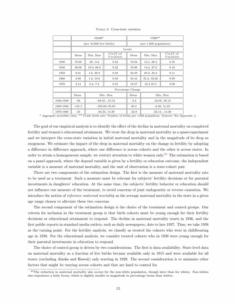
Table 3: Cross-state variation

MMR* CBR**

(per 10,000 live births) (per 1,000 population)

Levels

Mean Min, Max Coeff. ofV ariation

Mean Min, Max Coeff. ofV ariation

1930 70.68 49, 114 0.24 19.84 14.1, 28.4 0.16

1940 38.06 18.3, 68.8 0.32 18.98 14.4, 27.8 0.16

1950 8.81 1.8, 26.9 0.58 24.59 20.2, 32.4 0.11

1960 3.68 1.2, 10.6 0.56 24.44 21.2, 32.26 0.09

1970 2.14 0.4, 7.2 0.55 18.57 16.3 25.3 0.09

Percentage Change

Mean Min, Max Mean Min, Max

1940-1930 -46 -68.45, -15.54 -3.4 -34.05, 30.14

1960-1940 -131.5 -160.08,-56.83 30.4 -2.46, 51.23

1970-1960 -35 -83.33, 14.29 -23.9 -33.14, -14.29* Aggregate mortality rates. ** Crude birth rate: Number of births per 1,000 population. Sources: See Appendix A.

The goal of our empirical analysis is to identify the e!ect of the decline in maternal mortality on completedfertility and women’s educational attainment. We treat the drop in maternal mortality as a quasi-experimentand we interpret the cross-state variation in initial maternal mortality and in the magnitude of its drop asexogenous. We estimate the impact of the drop in maternal mortality on the change in fertility by adoptinga di!erence in di!erence approach, where one di!erence is across cohorts and the other is across states. Inorder to attain a homogeneous sample, we restrict attention to white women only.24 The estimation is basedon a panel approach, where the depend variable is given by a fertility or education outcome, the independentvariable is a measure of maternal mortality, and the unit of observation is a state-cohort pair.

There are two components of the estimation design. The first is the measure of maternal mortality rateto be used as a treatment. Such a measure must be relevant for subjects’ fertility decisions or for parentalinvestments in daughters’ education. At the same time, the subjects’ fertility behavior or education shouldnot influence our measure of the treatment, to avoid concerns of joint endogeneity or reverse causation. Weintroduce the notion of reference maternal mortality as the average maternal mortality in the state in a givenage range chosen to alleviate these two concerns.

The second component of the estimation design is the choice of the treatment and control groups. Ourcriteria for inclusion in the treatment group is that birth cohorts must be young enough for their fertilitydecisions or educational attainment to respond. The decline in maternal mortality starts in 1936, and thefirst public reports in standard media outlets, such as daily newspapers, date to late 1937. Thus, we take 1938as the turning point. For the fertility analysis, we classify as treated the cohorts who were in childbearingage in 1938. For the educational analysis, we consider treated cohorts who in 1938 were young enough fortheir parental investments in education to respond.

The choice of control group is driven by two considerations. The first is data availability. State level dataon maternal mortality as a fraction of live births became available only in 1915 and were available for allstates (excluding Alaska and Hawaii) only starting in 1929. The second consideration is to minimize otherfactors that might be varying across cohorts and that are hard to control for.

24The reduction in maternal mortality also occurs for the non-white population, though later than for whites. Non-whitesalso experience a baby boom, which is slightly smaller in magnitude in percentage terms than whites.

15

The next sections describe the estimation strategy in detail and discuss our main findings.

4.1 Fertility

We adopt a simple panel estimation approach, based on the following baseline regression equation:

Yst = &0 + &1ZZst + µs + 't + #Xst + (st, (9)

where Yst denotes the fertility outcome for birth year t and state s. Only females are included in the analysis.The variable ZZst is the measure of the treatment, the variable Xst denotes a set of controls, while µs and't correspond to state and cohort e!ects.

The baseline specification adopts reference maternal mortality, defined as the average maternal mortalityrate in the state at age 15-20 for each cohort, as a measure of the treatment:

ZZst = MMRrefst , (10)

where MMMrefst is reference maternal mortality for state s and cohort t. The choice of age range for

reference maternal mortality is motivated by the fact that the average age of first birth was well above 20for the cohorts we are interested in25, thus ensuring that the fertility behavior of the women included in theestimation does not a!ect their reference maternal mortality.

The baseline specification assumes women born in 1921-1940 were treated. Thus, the youngest treatedcohort was 17 in 1938. Women born between 1913 and 1921 are included in the control group. Thesensitivity analysis explores alternative definitions of reference maternal mortality and criteria for inclusionin the untreated and treated groups.

All specifications include a control for infant mortality, which has been found to be related importantlyto fertility (Preston, 1978, Haynes and Preston, 1991, Doepke, 2005). Thus, for the baseline specification,Xst = IMRref

st , where we define reference infant mortality as the mean infant mortality rate in the state atage 15-20 for each cohort. Progressively, we include a set of state level controls for possibly cohort specificeconomic, demographic, health, political and cultural indicators, which we describe in Section 4.1.2.

The coe"cient of interest is &1, which captures the cross-state average impact of the change in maternalmortality on the change in fertility in a comparison of treated (t") and untreated (t ) cohorts:

Yst! " Yst = &1 (ZZst! " ZZst) + 't! " 't + # (Xst! "Xst) .

A negative value of &1 implies that the decline in maternal mortality is associated with a rise in fertility.We are interested in the e!ects of the maternal mortality decline on completed fertility. We adopt the

statistic children ever born (CHBORN) at age 35-44 from the US Census 26, as the main fertility outcome, asthe median age of last birth for the cohorts included was 29. We also consider number of children under 13living in the household (NCHILD) at age 35-44 for robustness, though this measure may be biased downwardsdue to grown children having left the household. For some specification, we also consider the number ofchildren under 5 living in the household (NCHLT5) at age 23-32.

We conduct the estimation on three di!erent samples in a given age group: all women (All), married25Specifically, the average age of first birth was 24.6 for women born in 1911-1918, 23.7 for women born in 1921-1928 and

22.7 for women born in 1931-1938.26Fertility and education data are from the US Census. Appendix A provides a detailed description of the data.

16

women (Married), and married women with children (Married with Children). Since extra-marital fertilitywas small for the cohorts we consider, the results for all women can be seen a robustness check for thespecification that includes married women. Separate analysis of the sample of married women with childrenallows to assess the response of fertility on both the extensive and the intensive margins for married women.

Table 4 presents summary statistics for the sample we include in the baseline specification, including themean and standard deviation of the fertility outcomes in the treated and the control groups, the mean andstandard deviation of reference maternal mortality in the treatment and control groups and similar statisticsfor reference infant mortality. CHBORN is the fertility outcome that experiences the largest rise acrosscohorts, from 2.56 in the control group to 4.02 in the treatment group for married women.

Table 4: Fertility_ Baseline Specification

Mean 53.941 MeanSt. Dev. 7.9609 St. Dev.

Fertility Outcome CHBORN CHBORN CHBORN NCHILD NCHILD NCHILD NCHLT5 NCHLT5 NCHLT5Age 35-44 35-44 35-44 35-44 35-44 35-44 23-32 23-32 23-32

Sample Married All

Married with

Children Married All

Married with

Children Married All

Married with

Children

Mean 2.5584 2.4085 2.8232 1.9988 1.8258 2.4517 0.7344 0.5701 1.022St. Dev. 0.2044 0.2469 0.1966 0.2603 0.2562 0.2777 0.2052 0.1681 0.2715

Mean MeanSt. Dev. St. Dev.

Fertility Outcome CHBORN CHBORN CHBORN NCHILD NCHILD NCHILD NCHLT5 NCHLT5 NCHLT5Age 35-44 35-44 35-44 35-44 35-44 35-44 23-32 23-32 23-32

Sample Married All

Married with

Children Married All

Married with

Children Married All

Married with

Children

Mean 4.0172 3.8439 4.0688 2.4144 2.2378 2.736 0.9892 0.8629 1.1903St. Dev. 0.2862 0.352 0.2373 0.2459 0.2778 0.1966 0.1087 0.1009 0.1277

Control Group: Birth Years 1913-1920

Summary Statistics

7.1215

Reference Infant Mortality (Age 15-20)54.92313.1061

Reference Maternal Mortality (Age 15-20)

13.9442.8745

Reference Maternal Mortality (Age 15-20)

Reference Infant Mortality (Age 15-20)32.7648

Treated Group: Birth Years 1921-1940

4.1.1 Baseline Results

Table 5 presents the estimation results for the baseline specification (top panel, heading “Panel”). Thebaseline estimates suggest that the decline in maternal mortality had a strong positive e!ect on the rise infertility of treated cohorts relative to untreated cohorts. For CHBORN at age 35-44 in the specification thatincludes married women, the estimated coe"cient suggests that a decline in maternal mortality equal to

17

one standard deviation of pre-treatment maternal mortality is associated with a rise in CHBORN of 0.41 or16%. The cross-state average change in CHBORN between treated and untreated cohorts was 1.46, or 57%,thus a one standard deviation decline in maternal mortality can account for 28% of the change in fertility.The estimated coe"cient is significant at the 1% level and the specification explains 47% of the cross-statevariation in fertility.

The coe"cient on infant mortality is positive, consistent with a negative relation between the decline ininfant mortality and the change in fertility, and significant at the 1% level. A one standard deviation declinein infant mortality is associated with a change in fertility of "0.22. The inclusion of infant mortality doesnot a!ect the estimated coe"cient for maternal mortality.

The results for the All and Married with children samples are consistent with those for the sampleincluding all women. For all women, the estimated coe"cient, significant at the 1% level, implies thata one standard deviation decline in maternal mortality is associated with a 0.39 rise in fertility or 16%,which accounts for 27% of the actual rise in fertility. For the sample of married women with children, theestimated coe"cient drops in magnitude though it is still highly significant. A one standard deviation declinein maternal mortality is associated with a rise in fertility of 0.23 or 8% and accounts for 18% of the rise infertility between the treatment and control groups.

Results are similar for the other measures of fertility. For NCHILD at age 35-44 for the sample marriedwomen, the estimated coe"cient suggests that one standard deviation decline in maternal mortality isassociated with a 0.20 or 10% rise in the number of children in the household, which accounts for 47% ofthe actual rise in this statistic between treated and untreated cohorts. The coe"cient is significant at the1% level and the specification accounts for 27% of the variation in fertility across cohorts and across states.For NCHLT5 at age 23-32, a one standard deviation decline in maternal mortality is associated with a 0.07or 9% rise for married women, which accounts for 28% of the change in this variable between treated anduntreated cohorts. Similar results obtain for the sample of all women and the sample of married women withchildren.

18

Table 5: Fertility: Baseline Specification

Specification

Fertility Outcome CHBORN CHBORN CHBORN NCHILD NCHILD NCHILD NCHLT5 NCHLT6 NCHLT7

Age 35-44 35-44 35-44 35-44 35-44 35-44 23-32 23-32 23-32

Sample Married All

Married with

children Married All

Married with

children Married All

Married with

children

Constant 40.1315 31.9211 -54.1319 82.0808 84.8013 88.7148 22.5779 25.461 20.3772

t-stat 2.1925 1.8691 -2.0509 8.0239 8.9277 9.2827 3.571 4.667 2.591

MMRref

st (2) -0.0523 -0.049 -0.0291 -0.0257 -0.0254 -0.025 -0.0089 -0.011 -0.0052

t-stat -12.9721 -13.0167 -4.9969 -11.4064 -12.1148 -11.8614 -6.3752 -9.1696 -2.9991

IMRref

st (3) 0.0197 0.017 0.0146 0.0052 0.0038 0.0069 -0.0013 -0.0003 -0.0029

t-stat 3.7436 3.4659 1.9254 1.7851 1.3798 2.523 -0.734 -0.2007 -1.3059

Adj R-squared 0.4682 0.5151 0.252 0.2737 0.3405 0.2215 0.2649 0.3444 0.1857

R-squared 0.488 0.5331 0.2799 0.3007 0.365 0.2505 0.2922 0.3688 0.216

Predicted change in fertility

outcome for one st. dev.

change in pre-treatment

reference maternal mortality

0.41635507 0.3900841 0.23166219 0.20459513 0.20220686 0.1990225 0.07085201 0.0875699 0.04139668

Specification

Fertility Outcome CHBORN CHBORN CHBORN NCHILD NCHILD NCHILD NCHLT5 NCHLT6 NCHLT7

Age 35-44 35-44 35-44 35-44 35-44 35-44 23-32 23-32 23-32

Sample Married All

Married with

children Married All

Married with

children Married All

Married with

children

Constant 50.8226 42.359 -48.4887 97.8496 96.4153 112.5026 49.6386 45.8712 49.9368

t-stat 6.1342 5.4384 -1.814 7.7728 8.3717 10.1103 5.7799 6.132 4.7567

MMRref

st (2) -0.03 -0.029 -0.0007 -0.0256 -0.0237 -0.0299 -0.0172 -0.0159 -0.0155

t-stat -10.73 -11.0503 -0.0732 -6.0418 -6.1169 -7.9615 -5.9514 -6.3102 -4.3697

IMRref

st (3) 0.0118 0.0102 -0.0035 0.0068 0.0049 0.0104 0.001 0.0002 0.0007

t-stat 3.9821 3.6742 -0.364 1.5132 1.1869 2.6245 0.3305 0.0743 0.1771

Adj R-squared 0.5365 0.6623 0.054 0.2534 0.3408 0.2579 0.1269 0.1521 0.0933

R-squared 0.5607 0.6799 0.1033 0.2923 0.3751 0.2966 0.1724 0.1963 0.1405

Specification

Fertility Outcome CHBORN CHBORN CHBORN NCHILD NCHILD NCHILD NCHLT5 NCHLT6 NCHLT7

Age 35-44 35-44 35-44 35-44 35-44 35-44 23-32 23-32 23-32

Sample Married All

Married with

children Married All

Married with

children Married All

Married with

children

Constant -86.7468 -87.2234 -129.3648 23.0772 26.7125 30.0107 1.6488 -0.9456 9.2941

t-stat -5.9081 -6.359 -6.2309 2.8773 3.5876 3.9705 0.3326 -0.2194 1.5155

MMRpre

s*It (4) 0.014 0.013 0.0051 0.0088 0.0087 0.0078 0.0027 0.0031 0.0022

t-stat 9.5399 9.4177 2.4668 10.9151 11.6713 10.2307 5.4834 7.2697 3.6547

IMRref

st (3) -0.0012 -0.0027 0.0005 -0.0032 -0.0045 -0.002 -0.0045 -0.0045 -0.0042

t-stat -0.241 -0.5953 0.0713 -1.2129 -1.8361 -0.813 -2.7634 -3.1693 -2.0697

Adj R-squared 0.4391 0.4873 0.2414 0.2682 0.3357 0.2019 0.2591 0.3295 0.1884

R-squared 0.46 0.5064 0.2696 0.2954 0.3604 0.2315 0.2867 0.3544 0.2186

(1) Baseline specification. All regressions include state and cohort effects. Control group: 1913-1920. Treated group: 1921-1940.

(2) Reference maternal mortality is the average maternal mortality in the state at age 15-20 for each cohort.

(3) Reference infant mortality is the average infant mortality in the state at age 15-20.

(4) The instrument for reference MMR in each state is the average reference MMR for the control cohorts in each state.

Panel

Regression Results (1)

Panel, treated only

IV

19

4.1.2 Sensitivity

To assess the robustness of the baseline findings, we perform a variety of robustness checks.

Alternative Specifications We estimate equation (9) including only cohorts in the treatment group. Inthis specification, only the cross-state variation in maternal mortality is used to identify the impact of itsdecline on fertility for the treated cohorts. The states with lower maternal mortality can be interpreted ashaving experienced a larger treatment.

The results are presented in Table 5 (middle panel, heading “Panel, treated only”) and confirm those forthe baseline specification. For the married sample, the estimates imply that CHBORN at age 35-44 risesby 0.21 for a one standard deviation drop in maternal mortality. The coe"cient is significant at the 1%level, and the adjusted R-squared coe"cient is at 0.53, suggesting that this specification has considerableexplanatory power. The coe"cient on infant mortality is positive and significant, and the coe"cient formaternal mortality is robust to the inclusion of infant mortality in the regression. Results are similar forthe Married and Married with children samples. The estimation results for the other fertility measures alsoconfirm the findings for the baseline specification.

Instrumental Variables As a second robustness check, we estimate an instrumental variable version ofequation (9) where we use the average reference maternal mortality in the control group27, which we denotewith MMRpre

s , as an instrument for the magnitude of the treatment. In this case, ZZst is defined as:

ZZst = MMRpres ' Ipost

t , (11)

where the variable Ipostt indicates whether a birth cohort t belongs to the treatment group28. Given that a

larger initial value of maternal mortality corresponds to a larger decline, a positive value of the coe"cient&1 indicates that the decline in maternal mortality is associated with a rise in fertility between treated anduntreated cohorts.

The estimation results are presented in Table 5 (bottom panel, heading “IV”). The criteria for inclusionin the treatment and control groups are the same as for the baseline specification. The statistic MMRpre

s isa very strong instrument, as the correlation between MMRpre and the average decline in reference maternalmortality, between the treated and control cohorts, is 0.94 with a p-value of 0.00.

The estimates strongly confirm the panel estimates for all fertility outcomes and all samples. The esti-mated coe"cient for the married sample suggests that a one standard deviation decline in the instrumentis associated with an increase in CHBORN between the treated and control cohorts of 1.29 or 50%, whichaccounts for 89% of the actual change.

We also estimate a specification in which we instrument reference maternal mortality for the treatedcohorts with the mortality rates for the diseases that were most a!ected by the introduction of sulfa drugs,that is scarlet fever, pneumonia and influenza (Jayachandran, Lleras-Muney and Smith, 2009). We definethe reference sulfa related mortality rate, SulfaMRref

s , as the equally weighted average of the mortalityrates for scarlet fever, pneumonia and influenza at age 15-20 for each cohort t and state s. We then defineSulfapre

s to be the average of this indicator for all cohorts in the control group and use it as our instrumentin equation (11).

27Formally, MMRpres =

Pt$Control

MMRrefst

#Control , where Control is simply the set of cohorts in the control group.28Bleakley (2007) follows a similar approach to assess the e!ects of malaria eradication on fertility and educational attainment

in the American South.

20

The estimates, reported in Appendix D, Table 15, suggest a strong positive relation between the instru-ment for sulfa related mortalities and the change in fertility across cohorts, which implies that a larger declinein sulfa mortalities is associated with a larger rise in fertility across cohorts. The estimates are significantat the 1% level for all fertility measures and all samples, and explain close to 50% of the cross-state andcross-cohort variation.

Controls We now control progressively for several state level indicators to assess the potential for omittedvariable bias. The details on the definition and data sources for each indicator are reported in Appendix A.

We first consider a set of health indicators, including the male mortality rate (number of male deaths per100,000 population), the tuberculosis mortality rate (number of tuberculosis deaths per 100,000 population),the malaria mortality rate (male deaths per 100,000 population). The male mortality rate is an indicatorof general health conditions in the state29, while tuberculosis was the top cause of death for both men andwomen in the control group. We control for malaria since malaria eradication has been linked to a declinein fertility and educational attainment (Bleakley, 2007). Moreover, pregnant women are more likely to diefrom malaria, so variation in the incidence of malaria may account in part for the cross-state di!erences inmaternal mortality. Finally, we control jointly for mortality rates for diseases a!ected by the introductionof sulfa drugs (Jayachandran, Lleras-Muney and Smith, 2009), specifically scarlet fever, pneumonia andinfluenza (number of deaths per 100,000).

For each mortality rate we consider the reference value for the white population for each cohort, that isthe average in the state at age 15-20, with the age range equated to the one for reference maternal mortality.The results are displayed in Table 6 (left panel). We report estimates only for the sample of married womenfor the baseline specification. For all fertility measures, the e!ect of the decline in maternal mortality onfertility is robust to the inclusion of the health controls, both in terms of the magnitude and significance ofthe estimated coe"cient.

We next consider a set of economic and demographic controls. Group 1 includes state level personaldisposable income per capita and unemployment, interpreted as simple measures of the level of economicactivity. Group 2 includes the share of white population, the share of foreign born and the share of populationliving on a farm. These are basic demographic indicators, intended to capture some of the cross state variationin fertility behavior. Group 3 simply includes the share of employment in the public sector, as an indicator ofthe size of government in a particular state. Group 4 includes the share of employment in the health sector,as a proxie for the availability of medical services. The variable included in the regression is the averagevalue of the control at age 15-20 for each cohort. The results are displayed in Table 6 (middle panel). Theresults for CHBORN at age 35-44, which measures completed fertility, are robust to the inclusion of thesecontrols. The estimates are also robust for NCHILD and NCHLT5 for Groups 2-4, though controlling for theshare of employment in the health sector reduces the significance of the estimates. The estimated coe"cienton maternal mortality switches sign for NCHILD and NCHLT5 when controlling for economic conditions(Group 1). This suggests that economic conditions may a!ect the timing of fertility.

Finally, we control for a set of indicators intended to proxy for state level political and cultural preferences.Group 1 simply includes the literacy rate in 1930. This indicator is potentially linked to the ability to absorbmedical knowledge in the control group. Moreover, literacy is linked to the di!usion of basic schooling, whichwas related strongly to progressive values, including sensitivity regarding maternal health (Skopcol, 1992).

Group 2 includes an indicator of the acceptance of women’s su!rage, which can be linked to maternal29We exclude female deaths from this measure since it would be a!ected by maternal mortality.

21

health and fertility via multiple channels. In the aggregate, early access to voting rights for women mayincrease women’s political participation and heighten legislative intervention in the area of maternal andinfant health. Evidence in favor of this channel can be found in Miller (2008), who finds that child mortalitywas lower, and spending for public health higher, in states that introduced women’s su!rage early. Greaterpolitical representation for women may also improve women’s bargaining position within the household anddirectly influence maternal health outcomes by increasing household expenditures on obstetric care, which,as discussed in Section 2, entailed a significant financial outlay. We control for the variable “AcceptanceYear,” which corresponds to the date at which a state introduced or ratified women’s su!rage. A state withan earlier acceptance year is interpreted as having more openness towards women’s su!rage.

Group 3 includes indicators that capture state level spending on maternal and infant health under theauspices of the Sheppard-Towner Act of 1921-1929 and the Social Security Act of 1935. The Sheppard-Towner Act was a federal grant-in-aid program to incentivize educational activities promoting maternal andinfant health. Part 1, Title V of the Social Security Act provided federal funds, also on a grant-in-aid basis,to directly subsidize obstetric and infant care. The legislation is described in more detail in Appendix B. Weuse newly digitized data on state level appropriations and spending under these two programs to computethe total per capita federal payments received by each state. The data are described in detail in AppendixA.3.

The last indicator we consider, Group 4, is WWII mobilization rates. Mobilization rates could haveinfluenced fertility and education through a variety of channels. Acemoglu, Autor and Lyle (2004) findthat post-war labor market conditions were related significantly to mobilization rates. Specifically, unskilledsalaries were lower in states with high mobilization rates, which they interpret as a consequence of highparticipation of low skill women during the war years. Doepke, Hazan and Maoz (2007) argue that the risein labor force participation of married women during the war crowded out younger women from the labormarket after the war, causing them to opt for marriage and child bearing. Finally, mobilization rates maybe linked to the presence of war veterans eligible for GI Bill Benefits. The educational benefits were themost generous and popular program, and were enjoyed directly only by men (Altshuler and Blumin, 2009)30.Housing benefits were also substantial, and jointly with the education benefits may have a!ected householdincome and the demand for children. For example, higher household income may have discouraged wives’participation, thereby increasing their desired fertility.

We use state level mobilization rates from Acemoglu, Autor and Lyle (2004), interacted with an indicatorvariable, equal to 1 for the 1922-1928 birth cohorts, who were the greatest recipients of GI Bill educationalbenefits (Stanley, 2003, and Burns and Turner, 2002). The results are displayed in Table 6 (right panel).Indicators in Groups 1-3 are cohort invariant, and thus, we drop the state fixed e!ects from the regressionequation. We find that the estimates for all fertility measures are robust to the inclusion of these controls.Interestingly, we find that mobilization rates have a significant positive e!ect on completed fertility of the1921-1928 cohorts. However, the magnitude of this e!ect is small as a rise in mobilization rates of 0.05 raisesCHBORN at age 35-44 by 0.0431. By contrast, a one standard deviation decline in maternal mortality isassociated with a rise in the outcome of 0.24, in the specification that controls for mobilization rates.

Pre-Existing Trends To check for pre-existing trends, we also estimate equation (9) including onlycohorts that were not exposed to the decline in maternal mortality. The results are displayed in Table 16(top panel, heading “Fertility”) in Appendix D. Specifically, we consider women born in 1905"1915 (Control

30See footnote 32 for more details.31Mobilization ranged between 0.41 and 0.54, with a standard deviation of 0.034.

22

Tab

le6:

Fert

ility

_B

asel

ine

Spec

ifica

tion

Dep

en

den

t va

riab

leC

HB

OR

NN

CH

ILD

NC

HLT

5D

ep

en

den

t va

riab

leC

HB

OR

NN

CH

ILD

NC

HLT

5D

ep

en

den

t va

riab

leC

HB

OR

NN

CH

ILD

NC

HLT

5

Ag

e3

5-4

43

5-4

42

3-3

2A

ge

35

-44

35

-44

23

-32

Ag

e3

5-4

43

5-4

42

3-3

2

1:

Male

Mo

rtali

ty 1

: P

ers

on

al

Inco

me,

Un

em

p.

1:

Lite

racy

19

30

MM

Rre

f st (

4)

-0.0

51

3-0

.02

55

-0.0

08

7M

MR

ref st

(4

)-0

.02

49

0.0

11

60.

0024

MM

Rre

f st (

4)

-0.0

43

7-0

.02

6-0

.00

82

t-st

at-1

2.72

38-1

1.28

-6.2

34t-

stat

-5.0

038

4.98

851.

4132

t-st

at-1

2.36

29-1

2.63

01-6

.388

1

Ad

j R

-sq

uare

d0.

4716

0.27

390.

2657

Ad

j R

-sq

uare

d0.

4978

0.51

830.

3262

Ad

j R

-sq

uare

d0.

4309

0.16

040.

1302

2:

Su

lfa R

ela

ted

M

ort

ali

ty2

: W

hit

e,

Fore

ign

Bo

rn,

Farm

2:

Acc

ep

tan

ce o

f W

om

en

's S

uff

rag

e

MM

Rre

f st (

4)

-0.0

48

6-0

.02

59

-0.0

09

1M

MR

ref st

(4

)-0

.04

42

-0.0

10

6-0

.00

71

MM

Rre

f st (

4)

-0.0

45

3-0

.02

75

-0.0

08

2

t-st

at-1

2.13

45-1

1.39

24-6

.435

6t-

stat

-9.8

117

-4.7

059

-4.5

222

t-st

at-1

3.12

3-1

3.70

82-6

.461

8

Ad

j R

-sq

uare

d0.

4857

0.27

340.

2648

Ad

j R

-sq

uare

d0.

501

0.45

390.

3004

Ad

j R

-sq

uare

d0.

4443

0.18

130.

1375

3:

TB

Mo

rtali

ty3

: S

hare

Pu

bli

c3

: S

hep

pard

-To

wn

er

&

So

cial

Secu

rity

Act

MM

Rre

f st (

4)

-0.0

48

5-0

.02

59

-0.0

09

MM

Rre

f st (

4)

-0.0

47

1-0

.02

06

-0.0

07

4M

MR

ref st

(4

)-0

.04

37

-0.0

26

4-0

.00

77

t-st

at-1

2.13

51-1

1.36

23-6

.403

4t-

stat

-11.

507

-9.2

254

-5.1

906

t-st

at-1

2.53

37-1

3.10

43-6

.072

1

Ad

j R

-sq

uare

d0.

4866

0.27

330.

2646

Ad

j R

-sq

uare

d0.

480.

3252

0.27

63A

dj

R-s

qu

are

d0.

431

0.16

780.

1339

4:

Mala

ria

4:

Sh

are

Healt

h4

: M

ob

. R

ate

s a

pp

lied

to

19

22

-19

28

co

ho

rts

MM

Rre

f st (

4)

-0.0

56

3-0

.02

79

-0.0

09

8M

MR

ref st

(4

)-0

.03

37

-0.0

035

-0.0

022

MM

Rre

f st (

4)

-0.0

32

5-0

.02

72

-0.0

08

5

t-st

at-1

3.96

27-1

2.37

33-7

.021

3t-

stat

-7.4

441

-1.5

489

-1.4

165

t-st

at-8

.559

-12.

0909

-6.0

353

Ad

j R

-sq

uare

d0.

4826

0.29

260.

2745

Ad

j R

-sq

uare

d0.

4943

0.43

740.

3037

Mo

b.

Rate

0.8208

-0.0

453

-0.0

498

t-st

at6.

8513

-0.6

396

-1.1

235

Ad

j R

-sq

uare

d0.

4498

0.15

910.

1288

(1)

Bas

elin

e sp

ecifi

cation

. All

regr

essi

ons

incl

ude

stat

e an

d co

hort

eff

ects

. Con

trol

gro

up:

1913

-192

0. T

reat

ed g

roup

: 19

21-1

940.

(2)

Estim

ates

sho

wn

for

Mar

ried

sam

ple.

(3)

All

mor

talit

ies

are

aver

age

in t

he s

tate

at

age

15-2

0.(4

) Ref

eren

ce m

ater

nal m

orta

lity

is t

he a

vera

ge m

ater

nal m

orta

lity

in t

he s

tate

at

age

15-2

0 fo

r ea

ch c

ohor

t.

(5)

Onl

y in

clud

es t

ime

effe

cts.H

ealt

h (

3)

Eco

no

mic

an

d D

em

og

rap

hic

Sta

te C

hara

cteri

stic

s (5

)

Reg

ress

ion

Resu

lts

wit

h C

on

tro

ls

Pan

el S

peci

fica

tio

n (

1),

(2

)

23

Group I) and in 1910" 1915 (Control Group II). These women had mostly completed their fertility by 1938.Due to the fact that the state level maternal mortality data start in 1915 and are available for all the

states in the sample only starting in 1933, we extend the age range for reference maternal mortality. Theminimum age is set at 15 and the maximum age is the age in 1933 of the oldest included cohort (in thebaseline specification, the age range is 15-20). This implies that the included cohorts may be contributingwith their own fertility to reference maternal mortality. Given the systematic relation between parity andmaternal mortality risk, this could bias the estimates. The sign of the bias depends on average fertility,given that maternal mortality risk varies with parity (see footnote 8). Given the low fertility of cohorts inthis sample, an increase in fertility would be associated with a decline in the maternal mortality risk andlead to a negative bias in the coe"cient on maternal mortality in the regressions, potentially pointing to anegative relation between maternal mortality and fertility, even though it is not present. So the bias worksagainst the falsification exercise.

We limit attention to CHBORN at age 35-44 and find that the estimated coe"cient on reference maternalmortality is not significant in either control group. This suggests that there is no relation between maternalmortality and fertility across states for the untreated cohorts. To gauge whether the age range for thecalculation of reference maternal mortality influences this finding, we repeat the estimation for the treatmentgroup, using the same definition of reference maternal mortality as in the falsification exercise (TreatmentGroup in Table 16, top panel). We find that the baseline results are completely confirmed.

Included Cohorts and Reference Maternal Mortality We evaluate the sensitivity of the estimatesto the assumptions on reference maternal mortality and on the control and treated groups. Results forCHBORN at age 35-44 for Married women are presented in Table 7.

Columns 1-4 present estimates of equation (9) for di!erent assumptions on reference maternal mortality.Column 1 simply repeats the baseline estimates, for which reference maternal mortality is the average inthe state at age 15-20. The alternative age ranges we consider are 10-15 (column 2), 10-20 (column 3) and5-15 (column 4). Even if reference maternal mortality is sensitive to the age range, both the magnitudeand the significance of the estimated coe"cients are very robust to the definition of the age range, and theexplanatory power of the regression essentially is unchanged.

Columns 5-8 present estimates for alternative assumptions on the control and treatment groups. Column5 repeats the baseline results. For column 6, the control group is comprised by the 1910-1917 birth cohorts,while the treatment group corresponds to the 1918-1935 cohorts. For column 7, the 1910-1915 cohorts arethe control group, while the 1916-1930 cohorts are in the treatment group. Finally, for column 8, the controlgroup corresponds to the 1920-1929 birth years, and the treatment group to the 1930-1940 birth years. Onceagain, the estimation results confirm our baseline specification. The magnitude of the estimated coe"cient(in absolute value) on maternal mortality is mostly very close to the one for the baseline specification andsignificant at the 1% level.

4.1.3 Marriage Rates and Childlessness

This section examines the impact of the maternal mortality drop on marriage rates and childlessness.For the cohorts included in the analysis, extra-marital fertility was very small, and women who wished to

have children typically married. Therefore, if the decline in maternal mortality made childbearing desirablefor more women, it may have led to a rise in marriage rates. To examine this hypothesis, we estimate equation(9) using the percentage of women that are married (MARRIED) at age 23 as the dependent variable. The

24

Table 7: Included Cohorts and Reference Maternal Mortality

SpecificationFertility Outcome CHBORN CHBORN CHBORN CHBORN CHBORN CHBORN CHBORN CHBORNAge 35-44 35-44 35-44 35-44 35-44 35-44 35-44 35-44Sample Married Married Married Married Married Married Married MarriedColumn 1 2 3 4 5 6 7 8Control Cohorts 1913-1920 1910-1917 1910-1915 1920-1929Treated Cohorts 1921-1940 1921-1940 1921-1940 1921-1940 1921-1940 1918 - 1935 1916-1930 1930-1940Reference MMR Age 15-20 Age 10-15 Age 10-20 Age 5-15 Age 15-20 Age 15-20 Age 15-20 Age 15-20

Cross-state Average for Treated Cohorts 13.944 25.6366 19.8484 32.4996 13.944 22.3488 31.97 15.34

Constant 0.0145 0.0172 0.0186 0.0126 0.0125 -0.0041 -0.0144 0.0118t-stat 4.9044 6.3743 6.0394 3.9457 4.6696 -1.3434 -3.5734 4.4387

MMRrefst (3) 2.6344 2.5373 2.5284 2.6635 2.9486 3.6398 4.1507 2.7017

t-stat 28.4758 27.1616 26.0407 25.7019 28.8387 30.4086 27.6723 30.9591IMRref

st (4) -0.0203 -0.0157 -0.0192 -0.0121 -0.0248 -0.0204 -0.018 -0.0177t-stat -9.002 -9.7359 -9.4732 -6.5817 -15.028 -11.0093 -7.8296 -9.1321

Adj R-squared 0.5208 0.5184 0.5207 0.4913 0.5159 0.5669 0.5458 0.5287R-squared 0.5453 0.543 0.5452 0.5173 0.5335 0.584 0.568 0.5516Model p-value 0 0 0 0 0 0 0 0

(1) Panel estimates, including only treated cohorts. All regressions include state and cohort effects. Treated group: 1921-1940.(2) Baseline specification. All regressions include state and cohort effects. Control group: 1913-1920. Treated group: 1921-1940.(3) Reference maternal mortality is the average maternal mortality in the state at age 15-20 for each cohort. (4) Reference infant mortality is the average infant mortality in the state at age 15-20.

Panel (2)Panel, treated only (1)

results, displayed in Table 8, suggest that the decline in maternal mortality was associated with a significantrise in marriage rates. A one standard deviation decline in pre-treatment maternal mortality is associatedwith a 4% rise in the marriage rate in the baseline specification. The estimates for the IV specification arenot significant.

We also investigate the e!ect of the decline in maternal mortality on childlessness. Childlessness can belinked to maternal health, as the adverse health consequences of pregnancy may discourage childbearing. Wemeasure lifetime childlessness as the percentage by state of women with CHBORN=0 at age 35-44, whichwe denote with CHBORN_0. We perform the estimation on the samples All and Married. The resultsare displayed in Table 8. The panel estimates suggest no significant relation with CHBORN_0 for eithersample, despite the fact that childlessness for married women drops from 10% in the control group to 7% inthe treatment group. The IV estimates confirm these results.

25

Tab

le8:

Mar

riag

ean

dC

hild

less

ness

Sp

eci

fica

tio

nP

an

el

IVP

an

el

IVP

an

el

IVP

an

el

IVP

an

el

IVD

ep

en

den

t V

ari

ab

leM

AR

RIE

DM

AR

RIE

DC

HB

OR

N=

0C

HB

OR

N=

0C

HB

OR

N=

0C

HB

OR

N=

0N

CH

ILD

=0

NC

HIL

D=

0N

CH

ILD

=0

NC

HIL

D=

0A

ge

23

23

35

-44

35

-44

35

-44

35

-44

23

-32

23

-32

23

-32

23

-32

Sam

ple

All

All

All

All

Marr

ied

Marr

ied

All

All

Marr

ied

Marr

ied

Con

stan

t-5

.804

3-1

0.47

91-0

.782

70.

1126

2.58

30.

044

-12.

7715

0.17

8-4

.740

10.

1536

t-st

at-1

.967

1-4

.64

-0.7

041

8.39

322.

6075

3.67

01-1

2.02

7713

.313

6-3

.576

49.

6462

MM

Rre

f st (

2)

-0.0

03

1-0

.000

2-0

.000

40

0.00

02-0

.000

10

.00

18

-0.0

00

40

.00

11

-0.0

00

5t-

stat

-4.7

509

-0.8

125

-1.6

074

-0.1

607

0.74

92-0

.805

57.

7157

-4.3

838

3.72

05-4

.501

2IM

Rre

f st (

3)

0.00

290.

0016

0.00

06-0

.000

30.

0001

0.00

11-0

.000

1-0

.001

8-0

.000

6-0

.001

t-st

at3.

3705

2.17

051.

911

-1.7

026

0.50

227.

229

-0.3

732

-11.

0171

-1.4

618

-5.3

63A

dj

R-s

qu

are

d0.

4617

0.53

640.

3767

0.37

330.

2498

0.24

150.

303

0.23

670.

1654

0.16

83R-s

quar

ed0.

4817

0.55

360.

3999

0.39

620.

2777

0.26

920.

329

0.26

450.

1964

0.19

86P

red

icte

d c

han

ge i

n

fert

ilit

y o

utc

om

e f

or

on

e

st.

dev.

ch

an

ge i

n p

re-

treatm

en

t re

fere

nce

m

ate

rnal

mo

rtali

ty

0.04

0628

910.

0026

2122

0.00

3184

360

-0.0

0159

218

-0.0

0079

609

-0.0

1432

962

-0.0

0318

436

-0.0

0875

699

-0.0

0398

045

Dep

en

den

t V

ari

ab

leM

AR

RIE

DC

HB

OR

N=

0C

HB

OR

N=

0N

CH

ILD

=0

NC

HIL

D=

0S

am

ple

All

All

Marr

ied

All

Marr

ied

Ag

e2

33

5-4

43

5-4

42

3-3

22

3-3

2M

ean

0.93

620.

0999

0.10

70.

0807

0.10

33St.

Dev

.0.

2422

0.02

130.

0491

0.02

660.

0339

Mean

0.97

650.

107

0.07

40.

1014

0.10

27St.

Dev

.0.

093

0.04

910.

0219

0.02

60.

0292

(1)

Bas

elin

e sp

ecifi

cation

. All

regr

essi

ons

incl

ude

stat

e an

d co

hort

effec

ts.

Con

trol

gro

up:

1913

-192

0. T

reat

ed g

roup

: 19

21-1

940.

(2)

Ref

eren

ce m

ater

nal m

orta

lity

is t

he a

vera

ge m

ater

nal m

orta

lity

in t

he s

tate

at

age

15-2

0 fo

r ea

ch c

ohor

t.

(3)

Ref

eren

ce in

fant

mor

talit

y is

the

ave

rage

infa

nt m

orta

lity

in t

he s

tate

at

age

15-2

0. Tre

ate

d G

rou

p:

Bir

th Y

ears

19

21

-19

40

Reg

ress

ion

Resu

lts

(1)

Marr

iag

e R

ate

s

Co

ntr

ol

Gro

up

: B

irth

Years

19

13

-19

20

Su

mm

ary

Sta

tist

ics

Ch

ild

less

ness

26

4.1.4 Fertility by Education

We also estimate the e!ect of the decline in maternal mortality on fertility by education. We considerthe following fertility outcomes: CHBORN, NCHILD, and CHBORN_0 at age 35-44. We run separateregressions for women with college (COLL) and with high school (HS), for marriage status All and Married.

The results are displayed in Table 9. The estimated coe"cients on maternal mortality for the two fertilitymeasures are highly significant and have the same sign as the baseline specification for all education groups.The absolute and percentage rises in CHBORN and NCHILD were greater for college women, and theestimated coe"cient indeed predicts a greater rise in fertility for COLL women, relative to HS women.

For childlessness, as proxied by CHBORN_0 at age 35-44, the estimated coe"cient is close to zeroand insignificant for all samples except for married women with college. For this group it is positive andsignificant, suggesting that a one standard deviation decline in maternal mortality is associated with a 4%decline in childlessness for this group. For married high school women, the percentage who are childless atage 35-44 is smaller in the treated group relative to the control group, but it is not associated with the declinein maternal mortality. (Childlessness is approximately constant across the treated and control groups for thesample of All women.) One interpretation of this finding is that the opportunity cost of the adverse healthconsequences of pregnancy, including death, is greater for college educated women. Then, the reductionin pregnancy-related mortality would generate a greater reduction in childlessness for these women. Forrobustness we run also an IV version of all specifications. The IV estimates completely confirm the baselineresults.

27

Table 9: Fertility by Education

Specification

Fertility Outcome CHBORN NCHILD CHBORN=0 NCHILD=0 CHBORN NCHILD CHBORN=0 NCHILD=0Age 35-44 35-44 35-44 23-32 35-44 35-44 35-44 23-32Sample All All All All Married Married Married MarriedEducation COLL COLL COLL COLL COLL COLL COLL COLLConstant 76.0632 82.7137 -5.5398 20.2722 73.565 95.5935 -4.447 19.4051

t-stat 3.8264 4.639 -1.4437 5.118 3.4857 4.8955 -1.1949 5.2536MMRref

st (2) -0.025 -0.0302 0.0003 0.0029 -0.03 -0.0307 0.003 0.0009t-stat -5.7012 -7.6975 0.3065 3.2776 -6.4583 -7.146 3.7125 1.1511

IMRrefst (3) 0.0005 0.0018 0.0001 -0.0007 0.0033 0.0004 -0.0014 0.0003

t-stat 0.091 0.347 0.0804 -0.6363 0.5429 0.0681 -1.3117 0.267Adj R-squared 0.0988 0.1674 0.0264 0.42 0.1382 0.1537 0.0329 0.3229R-squared 0.1323 0.1983 0.0626 0.4415 0.1703 0.1852 0.0688 0.3481Model p-value 0 0 0.0013 0 0 0 0.0001 0

Predicted change in outcome for one st.

dev. drop in reference maternal mortality 0.1990225 0.24041918 -0.00238827 -0.02308661 0.238827 0.24439963 -0.0238827 -0.00716481

Fertility OutcomeMean 1.7944 1.3982 0.143 0.494 1.8551 1.7267 0.1576 0.3513St. Dev. 0.3343 0.3078 0.0701 0.0887 0.3691 0.3782 0.0777 0.0788

Mean 2.2739 2.038 0.161 0.2737 2.4751 2.3119 0.0972 0.1926St. Dev. 0.2545 0.2558 0.0473 0.0655 0.2732 0.2829 0.0269 0.0449

Specification

Fertility Outcome CHBORN NCHILD CHBORN=0 NCHILD=0 CHBORN NCHILD CHBORN=0 NCHILD=0Age 35-44 35-44 35-44 23-32 35-44 35-44 35-44 23-32Sample All All All All Married Married Married MarriedEducation HS HS HS HS HS HS HS HSConstant 20.0028 93.6221 -1.7209 5.1478 13.9662 94.3862 3.4676 5.6692

t-stat 2.2595 10.3468 -1.3575 1.9333 1.5158 9.5737 3.3163 2.7945MMRref

st (2) -0.0231 -0.0253 -0.0002 0.004 -0.0248 -0.0257 0 0.0025t-stat -11.8395 -12.6754 -0.6898 6.9026 -12.2026 -11.8523 -0.063 5.6061

IMRrefst (3) 0.0078 0.0023 0.0009 -0.0026 0.009 0.0031 0.0003 -0.0019

t-stat 3.0864 0.8826 2.4241 -3.455 3.4048 1.0939 0.9737 -3.2074Adj R-squared 0.5798 0.3986 0.3636 0.4086 0.568 0.3194 0.2718 0.3482R-squared 0.5955 0.4209 0.3873 0.4306 0.5841 0.3447 0.2988 0.3725Model p-value 0 0 0 0 0 0 0 0

Predicted change in outcome for one st.

dev. drop in reference maternal mortality 0.18389679 0.20141077 0.00159218 -0.0318436 0.19743032 0.20459513 0 -0.01990225

Fertility OutcomeMean 2.3074 1.8789 0.1002 0.3876 2.3366 2.0423 0.1008 0.2483St. Dev. 0.2832 0.2477 0.0228 0.0636 0.2821 0.2299 0.0237 0.043

Mean 2.9498 2.2493 0.1014 0.2487 3.0625 2.4105 0.0714 0.1514St. Dev. 0.3673 0.3043 0.0548 0.0714 0.3152 0.2756 0.0249 0.0463

(1) Baseline specification. All regressions include state and cohort effects. Control group: 1913-1920. Treated group: 1921-1940.(2) Reference maternal mortality is the average maternal mortality in the state at age 15-20 for each cohort. (3) Reference infant mortality is the average infant mortality in the state at age 15-20.

Treated Group: Birth Years 1921-1940

Treated Group: Birth Years 1921-1940

Panel

Regression Results (1)

Panel

Summary Statistics

Summary Statistics

Control Group: Birth Years 1913-1920

Control Group: Birth Years 1913-1920

28

4.2 Education

We now examine the impact of the decline in maternal mortality on female education. Educational attain-ment rose sharply throughout the twentieth century for both men and women. As shown in figure 3, collegegraduation rates were similar for men and women born between 1885 and 1910, after which male graduationrates rose at substantially faster rate for about 25 years. As discussed in Goldin, Katz and Kuziemko (2006),the scarcity of job opportunities during the Great Depression may have provided an incentive to attendcollege for men. Moreover, men were the exclusive recipients of the substantial educational benefit programcomprised in the GI Bill (Altshuler and Blumin, 2009)32. More than 10% of veterans born between 1922and 1928 achieved a bachelor’s of arts using GI benefits (Burns and Turner, 2002), and the gender disparityin access probably contributed to the clear widening of the gender di!erential in college graduation rates forthose cohorts.

Starting with the 1935 birth year, both the female/male ratio and the female-male di!erence in collegegraduation rate started rising sharply, inverting the trend prevailing for the 1910-1930 cohorts. Women bornin 1935 would mostly have started their schooling by 1941 and they would have graduated from high schoolby the mid 1950s. Their parents would have been aware of the progress in maternal health, and according tothe theory, they would have responded by increasing their investment in daughter’s education. Our empiricalanalysis seeks to examine the link between the decline in maternal mortality and various measures of women’seducational attainment.

32 Only 2% of the 16 million World War II veterans eligible for GI Bill educational benefits were female. The femalebeneficiaries received lower stipends than the male counterparts as their stipend did not rise with the number of dependents.See Altshuler and Blumin (2009) for more details.

29

-0.12

-0.10

-0.08

-0.06

-0.04

-0.02

0.00

0.00

0.10

0.20

0.30

0.40

0.50

0.60

0.70

0.80

0.90

1.00

1875 1880 1885 1890 1895 1900 1905 1910 1915 1920 1925 1930 1935 1940 1945 1950 1955

Birth Year

Females/Males (left axis)

Females-Males (right axis)

Figure 3: Gender di!erentials in college graduation rates.Source: Goldin (1997). Based on responses of individual aged 45-54 or 55-64. College graduation defined as college attendancefor 4 or more years.

The main measures of education attainment used in the analysis are the fraction of individuals with a highschool degree and the fraction with a college degree in the state. We also consider the fraction with at least 13years of schooling and the fraction with at least 16 years of schooling for robustness. Educational outcomesare measured at age 23-3233 and the estimation is conducted separately for All, Married and Married withchildren individuals. The estimation strategy is similar to the one employed for fertility, except here weinclude males in the analysis. Thus, in addition to the di!erences by state and by cohort, we also use thedi!erence by gender to identify the e!ect of the maternal mortality decline on female education.

We estimate the following equation:

Ysgt = &0 + &1ZZst ' Fg + µst + )gt + 'gs + #Xst + (gdt, (12)

where g = f, m stands for gender, and µst, )gt, 'gs correspond to state-cohort, gender-cohort and gender-stateinteractions34. As for fertility, the baseline specification is a panel regression that includes both treated anduntreated cohorts, with ZZst = MMRref

st , where MMRrefst corresponds to the average maternal mortality

in state, s, for cohort, t. A negative value of the estimated &1 implies a positive e!ect of a decline inpregnancy-related mortality on female educational attainment (relative to males) for the panel specification.

The assumptions on the age range for the calculation of reference maternal mortality and the inclusion33Given the small incidence of post-graduate and continuing education for the cohorts we consider, education was mostly

completed by age 23-32. We also consider educational outcomes at age 23, at age 35 and at age 35-44 as a robustness exercise.The findings are consistent with those for the baseline specification.

34This specification follows Jayachandran and Lleras-Muney (2008).

30

in the treated group di!er from those in the fertility analysis. Consistent with the model, we interpretthe change in educational outcomes as resulting from parental investments. Thus, we set the age range forreference maternal mortality to be 5"10, reflecting the age at which parents typically make choices on behalfof their children that a!ect lifetime educational attainment. The restricted age range for the calculation ofreference maternal mortality ensures that the subjects’ education cannot a!ect reference maternal mortality,thus removing the possibility of reverse causation.

For the baseline specification, individuals age -12 (born in 1950) to 5 (born in 1933) in 1938 are includedin the treated group. Thus, the treated cohorts are age 5 or younger in 1938, the year in which reports onthe decline in maternal mortality become available in the media. At age 5, parental investments in educationat all grade levels can potentially respond. The control group comprises birth years 1919-1932. The choiceof the control group is driven in part by data availability, as for the fertility analysis. We conduct sensitivityanalysis on the definition of treatment and controls groups.

Table 10 provides summary statistics on the control and treatment groups in the baseline specification.For both the treatment and control groups, high school graduation rates were higher for females than formales, while the converse is true for college graduation rates. Reference maternal mortality was 48.6 deathsfor 10,000 live births in the control group and 9.1 for the treatment group.

4.2.1 Baseline Results

The results for the baseline specification are presented in Table 11 (top panel, heading “Panel”). The estimatessuggest that the decline in maternal mortality had a strong positive e!ect on the female-male di!erentialin educational attainment for all educational outcomes and all samples. The estimated coe"cients are allsignificant at the 1% level and imply sizable e!ects. The estimates predict that a one cross-state standarddeviation decline in reference maternal mortality in the control group is associated with a 0.018 rise in thefemale-male college graduation di!erential, a 49% rise from the average cross-state di!erential for the controlgroup, which was -0.0358. The adjusted R-squared suggests that the baseline specification explains 0.39 ofthe cross-state and cross-cohort variation.

The results for high school graduation are similarly strong. A decline in maternal mortality correspondingto a one standard deviation in the control group is associated with a 0.044 (or 81%) rise in the female-maledi!erential in high school graduation rate for the sample of all individuals, with an adjusted R-squared of0.45. The sample of married and married with children individuals delivers similar results.

4.2.2 Sensitivity

To assess the robustness of these findings, we conduct a sensitivity analysis which parallels the one for thefertility estimates.

Alternative Specifications and Instrumental Variables We consider a specification that only in-cludes treated cohorts and an instrumental variable specification, where, as for fertility, we define ZZst =MMRpre

s ' Ipostt , where MMRpre

s is average reference maternal mortality in the control group and thevariable Ipost

t indicates whether a birth cohort t belongs to the treatment group. For the IV specification, apositive estimated value of &1 is consistent with a positive e!ect of the drop in maternal mortality on femaleeducational attainment (relative to males).

The results are displayed in Table 11 and strongly confirm the findings for the baseline specification. Thepanel estimates for the treated cohorts suggest that a one standard deviation decline in maternal mortality

31

Tab

le10

:E

duca

tion

_B

asel

ine

Spec

ifica

tion

Mean

48.5588

St.

Dev.

7.3353

Ed

uca

tio

nal

Att

ain

men

t at

ag

e

23

-32

CO

LLC

OLL

CO

LLH

SH

SH

SH

G1

6H

G1

6H

G1

6H

G1

3H

G1

3H

G1

3

Sam

ple

All

Marr

ied

Marr

ied

w

ith

ch

ild

ren

All

Marr

ied

Marr

ied

w

ith

ch

ild

ren

All

Marr

ied

Marr

ied

w

ith

ch

ild

ren

All

Marr

ied

Marr

ied

w

ith

ch

ild

ren

Mean

Fem

ale

0.0423

0.0359

0.0303

0.2268

0.2287

0.2169

0.0733

0.0605

0.0502

0.1968

0.1777

0.1588

St.

Dev.

Fem

ale

0.0147

0.0119

0.0088

0.0322

0.0329

0.0286

0.0236

0.0188

0.0155

0.0512

0.0452

0.0407

Mean

Male

0.0781

0.0725

0.0643

0.1726

0.1763

0.1648

0.1195

0.111

0.0974

0.2463

0.2238

0.1992

St.

Dev.

Male

0.0218

0.0174

0.015

0.025

0.0258

0.0235

0.0345

0.0311

0.0258

0.0571

0.0524

0.0513

Mean

9.1113

St.

Dev.

2.0244

Ed

uca

tio

nal

Att

ain

men

t at

ag

e

23

-32

CO

LLC

OLL

CO

LLH

SH

SH

SH

G1

6H

G1

6H

G1

6H

G1

3H

G1

3H

G1

3

Sam

ple

All

Marr

ied

Marr

ied

w

ith

ch

ild

ren

All

Marr

ied

Marr

ied

w

ith

ch

ild

ren

All

Marr

ied

Marr

ied

w

ith

ch

ild

ren

All

Marr

ied

Marr

ied

w

ith

ch

ild

ren

Mean

Fem

ale

0.1373

0.1264

0.1033

0.4538

0.4679

0.4745

0.1373

0.1264

0.1033

0.2952

0.2826

0.2533

St.

Dev.

Fem

ale

0.0619

0.0595

0.0355

0.0538

0.0558

0.0493

0.0619

0.0595

0.0355

0.077

0.0773

0.0588

Mean

Male

0.2045

0.196

0.1567

0.3668

0.3815

0.4069

0.2045

0.196

0.1567

0.3811

0.3656

0.3161

St.

Dev.

Male

0.0644

0.0629

0.05

0.0513

0.0531

0.0593

0.0644

0.0629

0.05

0.0758

0.0731

0.0714

Refe

ren

ce M

ate

rnal M

ort

ality

(A

ge 5

-10

)

Refe

ren

ce M

ate

rnal M

ort

ality

(A

ge 5

-10

)

Co

ntr

ol G

rou

p:

Bir

th Y

ears

19

19

-19

32

Tre

ate

d G

rou

p:

Bir

th Y

ears

19

33

-19

50

Su

mm

ary

Sta

tist

ics

32

Tab

le11

:E

duca

tion

_B

asel

ine

Spec

ifica

tion

Sp

eci

fica

tio

n

Ed

uca

tio

nal A

ttain

men

t at

ag

e 2

3-3

2C

OLL

CO

LLC

OLL

HS

HS

HS

HG

16

HG

16

HG

16

HG

13

HG

13

HG

13

Sam

ple

Marr

ied

All

Marr

ied

wit

h

child

ren

Marr

ied

All

Marr

ied

wit

h

child

ren

Marr

ied

All

Marr

ied

wit

h

child

ren

Marr

ied

All

Marr

ied

wit

h

child

ren

Con

stan

t0.

0894

0.09

170.

0819

0.27

240.

2613

0.26

20.

1089

0.11

410.

0991

0.22

870.

2463

0.21

21

t-st

at5.

8598

6.38

515.

3709

12.5

099

12.7

325

10.3

643

7.11

088.

0123

6.32

1810

.523

511

.962

19.

2842

MM

Rre

f st *

F g (

2)

-0.0

02

3-0

.00

24

-0.0

01

9-0

.00

63

-0.0

06

-0.0

06

8-0

.00

17

-0.0

01

6-0

.00

14

-0.0

02

7-0

.00

25

-0.0

02

4

t-st

at-2

3.46

51-2

6.03

24-1

9.37

89-4

4.25

02-4

4.64

59-4

1.18

53-1

6.65

6-1

7.34

1-1

3.27

57-1

8.85

79-1

8.58

46-1

6.40

66

Ad

j R

-sq

uare

d0.

3105

0.35

860.

2047

0.43

620.

4461

0.38

520.

2844

0.32

490.

1739

0.24

990.

2821

0.18

34

R-s

quar

ed0.

332

0.37

870.

2295

0.45

380.

4635

0.40

440.

3068

0.34

60.

1997

0.27

330.

3046

0.20

89

Pre

dic

ted

ch

an

ge in

fem

ale

-m

ale

dif

fere

nti

al fo

r 1

st

.dev.

ch

an

ge in

pre

-tr

eatm

en

t re

fere

nce

MM

R0

.01

68

71

19

0.0

46

21

23

90

.01

24

70

01

0.0

19

80

53

10

.01

76

04

72

0.0

44

01

18

0.0

11

73

64

80

.01

83

38

25

0.0

13

93

70

70

.04

98

80

04

0.0

10

26

94

20

.01

76

04

72

Sp

eci

fica

tio

n

Ed

uca

tio

nal A

ttain

men

t at

ag

e 2

3-3

2C

OLL

CO

LLC

OLL

HS

HS

HS

HG

16

HG

16

HG

16

HG

13

HG

13

HG

13

Sam

ple

Marr

ied

All

Marr

ied

wit

h

child

ren

Marr

ied

All

Marr

ied

wit

h

child

ren

Marr

ied

All

Marr

ied

wit

h

child

ren

Marr

ied

All

Marr

ied

wit

h

child

ren

Con

stan

t0.

143

0.14

580.

1292

0.39

410.

3765

0.4

0.14

30.

1458

0.12

920.

288

0.29

560.

262

t-st

at7.

7984

9.37

816.

0428

24.3

242

26.7

975

18.1

037

7.79

849.

3781

6.04

2812

.111

413

.904

39.

3125

MM

Rre

f st *

F g (

2)

-0.0

05

5-0

.00

57

-0.0

04

4-0

.00

08

-0.0

00

4-0

.00

15

-0.0

05

5-0

.00

57

-0.0

04

4-0

.00

93

-0.0

09

3-0

.00

8

t-st

at-1

4.08

-17.

3514

-9.6

583

-2.3

79-1

.489

4-3

.179

6-1

4.08

-17.

3514

-9.6

583

-18.

3508

-20.

5435

-13.

4722

Ad

j R

-sq

uare

d0.

4641

0.56

110.

2356

0.48

910.

5536

0.29

160.

4641

0.56

110.

2356

0.45

990.

5276

0.29

15

R-s

quar

ed0.

4939

0.58

550.

2781

0.51

750.

5784

0.33

10.

4939

0.58

550.

2781

0.48

990.

5538

0.33

08

Sp

eci

fica

tio

n

Ed

uca

tio

nal A

ttain

men

t at

ag

e 2

3-3

2C

OLL

CO

LLC

OLL

HS

HS

HS

HG

16

HG

16

HG

16

HG

13

HG

13

HG

13

Sam

ple

Marr

ied

All

Marr

ied

wit

h

child

ren

Marr

ied

All

Marr

ied

wit

h

child

ren

Marr

ied

All

Marr

ied

wit

h

child

ren

Marr

ied

All

Marr

ied

wit

h

child

ren

Con

stan

t0.

0837

0.08

580.

077

0.25

70.

2465

0.24

510.

1049

0.11

030.

0959

0.22

20.

240.

206

t-st

at5.

3509

5.79

494.

9571

10.8

468

11.0

196

8.99

296.

7742

7.64

326.

0732

10.0

447

11.4

672

8.90

32M

MR

pre

s*F

g*

I t (

3)

0.0

01

80

.00

19

0.0

01

50

.00

48

0.0

04

60

.00

52

0.0

01

30

.00

12

0.0

01

10

.00

20

.00

19

0.0

01

9

t-st

at19

.341

221

.389

515

.842

34.3

3434

.511

832

.103

614

.068

714

.588

911

.272

115

.524

915

.286

713

.575

6

Ad

j R

-sq

uare

d0.

2748

0.31

820.

1745

0.33

20.

3411

0.28

460.

2668

0.30

670.

1611

0.22

370.

2576

0.16

19

R-s

quar

ed0.

2974

0.33

950.

2003

0.35

290.

3617

0.30

690.

2897

0.32

830.

1873

0.24

790.

2808

0.18

81

(1)

Bas

elin

e sp

ecifi

cation

. All

regr

essi

ons

incl

ude

fully

inte

ract

ed s

tate

, ge

nder

and

coh

ort

effe

cts.

Con

trol

gro

up:

1919

-193

2. T

reat

ed g

roup

: 19

33-1

950.

(2)

Ref

eren

ce m

ater

nal m

orta

lity

is t

he a

vera

ge m

ater

nal m

orta

lity

in t

he s

tate

at

age

5-10

for

eac

h co

hort

. (3

) Th

e in

stru

men

t fo

r re

fere

nce

MM

R in

eac

h st

ate

is t

he a

vera

ge r

efer

ence

MM

R for

the

con

trol

coh

orts

in e

ach

stat

e.

Pan

el

Pan

el,

tre

ate

d o

nly

IV

Reg

ress

ion

Resu

lts

(1)

33

in the treatment group is associated with 0.012 rise in the female-male di!erential in college graduationrates (middle panel, heading “Panel, treated cohorts”). The mean value of this di!erential in the treatmentgroup is -0.069. The estimates are not as big for high school graduation, but are still highly significant withconsiderable explanatory power. The IV estimates (bottom panel, heading “IV”) are consistent with theother specifications.

Pre-Existing Trends To gauge the presence of pre-existing trends, we estimate equation (12) for thecohorts in the control group. The results are displayed in Appendix D, Table 16 (bottom panel, heading“Education”). We limit attention to HS and COLL at age 23-32. We consider two samples of untreatedcohorts, comprising birth years 1910-1917 (Control Group I, age 21 in 1931-1938) and 1918-1925 (ControlGroup II, age 21 in 1939-1946).

As for fertility, we extend the definition of reference maternal mortality, since the state level maternalmortality data start in 1915, and are available for all the states in the sample only starting in 1933. Whilein the baseline specification, the age range for reference maternal mortality is 5-10, here the minimum ageis 5 and the maximum is the age in 1933 for the oldest cohort included in the regression (age 23 for ControlGroup I and age 15 for Control Group II). The change in the reference maternal mortality implies thatthe women included in the analysis potentially contribute to the measure of reference maternal mortalitywith their childbearing behavior. Specifically, if higher female education is associated with lower maternalmortality, this would lead us to find a negative relation between these two variables even in the controlgroup. For consistency, we also repeat the estimation for the treated cohorts in the baseline specificationusing the age range for reference maternal mortality used in the falsification exercise.

We find that the estimated coe"cient on reference maternal mortality is insignificant or of the wrongsign for COLL for both control groups. This suggests that there is no relation between maternal mortalityand COLL across states for the untreated cohorts. For HS we find a negative and significant coe"cient forboth control groups and both samples. This finding may be due to reverse causation, as discussed above.The estimates for the treatment group with reference maternal mortality defined as for Control Group I (age5-23), confirm the results in the main analysis.

Reference Maternal Mortality and Included Cohorts We now investigate the sensitivity of ourfindings to the assumptions on the age range for reference maternal mortality and the treatment and controlgroups, concentrating on college graduation rates. The results are reported in Table 12.

Columns 1-4 explore the sensitivity to the definition of reference maternal mortality. We do so to allowdi!erent time lags between the observation of maternal mortality and the influence of maternal mortality onparental investments in daughters’ education. For the baseline specification, reference maternal mortalityis the average in the state at age 5-14 (column 1). Here, we also consider: age 0 to 15 (column 2), 5to 10 (column 3) and -5 to 5 (column 4). Since the alternative assumptions mainly a!ect the value ofreference maternal mortality for the treated cohorts, we report only estimates for this group. We find thatthe alternative assumptions confirm our baseline results.

Columns 5-9 examine the sensitivity to the definition of control and treatment group. Column 5 reportsthe baseline results. Column 6 maintains the assumption on the control cohorts (born in 1921-1932) andassumes individuals born in 1933-1940 are treated, to explore whether the female-male di!erential in collegegraduation rates rose immediately as maternal mortality declined. We then change both the treatment andthe control groups relative to the baseline specification. Specifically, we assume that the treated cohorts

34

comprise birth years 1940-1950 (column 7), 1945-1955 (column 8), 1950-1960 (column 9) and take theprevious 10 birth years as a control group in each case. The estimation results confirm the findings for thebaseline specification. The absolute value of the estimated coe"cient on reference maternal mortality islargest for the the 1950-1960 cohorts and smallest for the 1933-1950 cohorts.

Controls We use the same set of controls as in the fertility analysis, described in Section 4.1.2.The health indicators are computed as an average of the corresponding mortality rate at age 5-10 for

each cohort, to ensure that the reference age is the same as for maternal mortality. In addition to Groups1-4 included in the fertility analysis, we also control for infant mortality (not interacted with gender), whichcorresponds to Group 535. The results are displayed in Table 13 (first panel) and suggest that the estimatesfor education are robust to the inclusion of these controls. Consistent with the literature (Murphy, Simon andTamura, 2005), we find that a decline in infant mortality is associated with a rise in educational attainment.

We also find that the education results are robust to the inclusion of the economic and demographiccontrols (second panel) and the controls for state level cultural and political preferences (third panel). Forthis analysis, we interact mobilization rates with a female dummy, given that GI Bill education benefits wereavailable only for male veterans (see footnote 32). Interestingly, we find that mobilization rates had a strongnegative e!ect on the female-male di!erential in both high school and college graduation rates. An increasein mobilization rates of 0.05 is associated with a decline of the female-male di!erential in graduate rates by0.02 for high school and 0.01 for college.

Finally, we control for access to oral contraception for unmarried women for the treated cohorts. Asshown by Goldin and Katz (2002), access to contraception for unmarried women had a positive impact ontheir educational attainment, which could have exerted an independent negative e!ect on fertility. We useBailey’s (2006) coding of legal access to oral contraception for unmarried women, interacted with a femaledummy and an indicator equal to 1 for cohorts in the treated group, since only women in these cohortswould have had access. We find that including the control for early legal access to oral contraception doesnot a!ect the estimates on maternal mortality.

4.3 Baby Bust

We also estimate a specification intended to capture the relation between the maternal mortality decline andthe baby bust. As we have shown, the decline in maternal mortality had a positive e!ect on educationalattainment of women (relative to men) for the birth cohorts that were young enough when the decline inmaternal mortality took place. The fertility choice model analyzed in Section 3 predicts a negative relationbetween mothers’ education and desired fertility. This suggests that the maternal mortality decline mayhave contributed in part to the baby bust by increasing educational attainment for these cohorts, relative towomen who had completed their education by the time maternal mortality started to decline.

To investigate this hypothesis, we estimate equation (9) including the cohorts whose fertility or educationresponded to the decline in maternal mortality, based on our previous analysis, that is birth years 1921-1950.Recall that birth years 1921-1940 responded positively with fertility to the decline in maternal mortality(relative to the 1913-1920 cohorts), while birth years 1933-1950 responded positively with education (relativeto the 1919-1932 cohorts). To assess whether the youngest cohorts have lower fertility than the older cohortsin this group, we designate the 1941-1950 cohorts as treated36, and estimate an IV specification, where the

35The baseline specification for fertility already controls for infant mortality.36For robustness, we also repeat the analysis assuming women born in 1933-1950 and 1946-1950 are treated and find similar

35

Tab

le12

:Se

nsitiv

ity:

Tre

ated

and

Con

trol

Gro

ups,

Ref

eren

ceM

ater

nalM

orta

lity

Sp

eci

fica

tio

nEd

uca

tio

n O

utc

om

eC

OLL

CO

LLC

OLL

CO

LLC

OLL

CO

LLC

OLL

CO

LLC

OLL

Sam

ple

All

All

All

All

All

All

All

All

All

Ag

e2

3-3

22

3-3

22

3-3

22

3-3

22

3-3

22

3-3

22

3-3

22

3-3

22

3-3

2C

olu

mn

12

34

56

78

9C

on

tro

l C

oh

ort

s19

19-1

932

1919

-193

21

93

0-1

93

91

93

5-1

94

41

94

0-1

94

9Tre

ate

d C

oh

ort

s19

33-1

950

1933

-195

019

33-1

950

1933

-195

019

33-1

950

19

33

-19

40

19

40

- 1

95

01

94

5-1

95

51

95

0-1

96

0R

efe

ren

ce M

MR

Age

5-1

4A

ge 0

-15

Ag

e 5

-10

Ag

e -

5-5

Age

5-1

4Age

5-1

4Age

5-1

4Age

5-1

4Age

5-1

4C

ross

-sta

te A

vera

ge

for

Co

ntr

ol C

oh

ort

s48

.558

848

.558

834

.943

718

.204

98.

4337

Cro

ss-s

tate

Ave

rag

e

for

Tre

ate

d C

oh

ort

s9.

1113

13.3

392

11.4

7429

.526

39.

1113

9.07

562.

6726

2.21

171.

6517

Con

stan

t0.

1458

0.14

670.

1461

0.14

780.

0917

0.09

510.

1736

0.11

310.

1764

t-st

at9.

3781

9.55

159.

4479

9.78

26.

3851

6.31

492.

4467

2.28

774.

4615

MM

Rre

f st (

2)

-0.0

057

-0.0

045

-0.0

046

-0.0

028

-0.0

024

-0.0

024

-0.0

043

-0.0

077

-0.0

149

t-st

at-1

7.35

14-1

8.67

72-1

7.90

68-2

0.37

82-2

6.03

24-2

3.14

03-7

.028

5-9

.031

7-9

.455

8A

dj

R-s

qu

are

d0.

5611

0.57

150.

5654

0.58

520.

3586

0.32

440.

2764

0.49

30.

6938

R-s

quar

ed0.

5855

0.59

530.

5896

0.60

820.

3787

0.34

560.

6401

0.74

780.

8477

Mod

el p

-val

ue0

00

00

00.

0029

00

Pan

el,

tre

ate

d o

nly

(1

)P

an

el

(1)

36

Tab

le13

:E

duca

tion

_B

asel

ine

Spec

ifica

tion

Ed

uca

tio

nal

Att

ain

men

t at

ag

e 2

3-

32

HS

CO

LL

Ed

uca

tio

nal

Att

ain

men

t at

ag

e

23

-32

HS

CO

LLEd

uca

tio

nal

Att

ain

men

t at

ag

e 2

3-3

2H

SC

OLL

Ed

uca

tio

nal

Att

ain

men

t at

ag

e

23

-32

HS

CO

LLS

am

ple

Marr

ied

Marr

ied

Marr

ied

Marr

ied

Marr

ied

Marr

ied

Marr

ied

Marr

ied

1:

Male

Mo

rtali

ty 1

: P

ers

on

al

Inco

me,

Un

em

p.

1:

Lite

racy

19

30

Earl

y Le

gal

Acc

ess

to

Pil

l M

MR

ref st

*F

g (

2)

-0.0

05

5-0

.00

2M

MR

ref st

*F

g (

2)

-0.0

05

4-0

.00

09

MM

Rre

f st *

Fg

(2

)-0

.00

36

0.00

01M

MR

ref st

*F

g (

2)

-0.0

07

3-0

.00

26

t-st

at-3

6.91

22-1

8.94

52t-

stat

-33.

9725

-9.2

148

t-st

at-2

2.96

531.

2996

t-st

at-2

3.30

19-1

1.59

05A

dj

R-s

qu

are

d0.

4387

0.31

05

Ad

j R

-sq

uare

d0.

465

0.32

26A

dj

R-s

qu

are

d0.

4679

0.48

11A

dj

R-s

qu

are

d0.

5639

0.56

94

2:

Su

lfa r

ela

ted

2:

Wh

ite,

Fore

ign

B

orn

, Fa

rm2

: A

ccep

tan

ce o

f W

om

en

's S

uff

rag

eM

MR

ref st

*F

g (

2)

-0.0

02

10

.00

03

MM

Rre

f st *

Fg

(2

)-0

.00

38

-0.0

00

3M

MR

ref st

*F

g (

2)

-0.0

06

3-0

.00

21

t-st

at-1

3.88

793.

0709

t-st

at-2

5.07

68-3

.010

2t-

stat

-44.

5071

-23.

1226

Su

lfa r

ela

ted

-0.0

05

2-0

.00

33

Ad

j R

-sq

uare

d0.

5833

0.54

47A

dj

R-s

qu

are

d0.

4387

0.42

56t-

stat

-41.

4333

-36.

2608

Ad

j R

-sq

uare

d0.

6397

0.51

87

3:

Mala

ria

3:

Sh

are

Pu

bli

c3

: S

hep

pard

-To

wn

er

&

So

cial

Secu

rity

Act

MM

Rre

f st *

Fg

(2

)-0

.00

58

-0.0

02

1M

MR

_st

*F_

g-0

.00

48

-0.0

00

5M

MR

ref st

*F

g (

2)

-0.0

06

3-0

.00

22

t-st

at-3

9.39

49-2

0.52

94t-

stat

-29.

7395

-5.1

892

t-st

at-4

3.71

95-2

1.98

33A

dj

R-s

qu

are

d0.

4556

0.31

78A

dj

R-s

qu

are

d0.

4881

0.49

61A

dj

R-s

qu

are

d0.

441

0.33

56

4:

TB

4:

Sh

are

Healt

h

4:

Mo

b.

Rate

s a

pp

lied

to

19

22

-19

28

co

ho

rts,

in

tera

cted

wit

h g

en

der

MM

Rre

f st *

Fg

(2

)-0

.00

21

0.0

00

3M

MR

ref st

*F

g (

2)

-0.0

04

7-0

.00

02

MM

Rre

f st *

Fg

(2

)-0

.00

54

-0.0

02

4t-

stat

-14.

0974

3.01

94t-

stat

-28.

5397

-1.5

366

t-st

at-3

0.70

4-1

9.13

84TB

-0.0

02

6-0

.00

17

Ad

j R

-sq

uare

d0.

485

0.54

19M

ob

. R

ate

*F_

g-0

.17

52

0.00

73t-

stat

-40.

9281

-36.

2331

-8.8

041

0.51

82A

dj

R-s

qu

are

d0.

6366

0.51

85A

dj

R-s

qu

are

d0.

4501

0.31

03

5:

Infa

nt

Mo

rtali

ty7

: M

ob

. R

ate

s a

pp

lied

to

19

22

-19

28

co

ho

rts

MM

Rre

f st *

Fg

(2

)-0

.00

45

-0.0

001

MM

Rre

f st *

Fg

(2

)-0

.00

45

-0.0

01

6t-

stat

-27.

1509

-1.1

563

t-st

at-3

3.01

56-1

4.95

18IM

R_

t-0

.00

37

-0.0

04

8M

ob

. R

ate

-0.3

45

3-0

.14

83

t-st

at-1

7.91

78-3

7.62

86t-

stat

-31.

5435

-17.

6226

Ad

j R

-sq

uare

d0.

494

0.53

61A

dj

R-s

qu

are

d0.

5752

0.37

42

(1)

Bas

elin

e sp

ecifi

cation

. I

nclu

des

stat

e/tim

e, f

emal

e/tim

e, f

emal

e/st

ate

inte

ract

ions

. Con

trol

gro

up:

1919

-193

2. T

reat

ed g

roup

: 19

33-1

950.

(2)

Ref

eren

ce m

ater

nal m

orta

lity

is t

he a

vera

ge m

ater

nal m

orta

lity

in t

he s

tate

at

age

5-10

for

eac

h co

hort

. (3

) Es

tim

ates

sho

wn

for

Mar

ried

sam

ple.

(4)

All

mor

talit

ies

are

aver

age

in t

he s

tate

at

age

5-10

.

Reg

ress

ion

Resu

lts

wit

h C

on

tro

ls

Pan

el S

peci

fica

tio

n (

1)

(3)

Healt

h (

4)

Eco

no

mic

an

d D

em

og

rap

hic

Sta

te C

hara

cteri

stic

sC

on

tro

ls f

or

Tre

ate

d C

oh

ort

s

37

instrument is the average reference maternal mortality (at age 15-20) in the state for the birth years 1913-1920 (the untreated cohorts for the main fertility specification). This approach is consistent with the theory,since the instrument proxies for the magnitude of the maternal mortality decline that influenced fertility forthe control cohorts and parental investments in education for the treated cohorts. For robustness, we alsoconsider a specification in which the control group is comprised of the 1921-1945 cohorts and the treatedgroup of the 1946-1950 cohorts, and a specification in which the 1933-1940 cohorts are in the control groupand the 1941-1950 cohorts in the treatment group.

The findings are displayed in Table 14. We focus on CHBORN at age 35-44, and consider the samples ofAll, Married and Married with children women. The bottom panel presents summary statistics for the fertilityoutcome for the control and treated cohorts in each specification. Completed fertility for married women isabout 30% lower for the treated cohorts relative to the control cohorts, in all three specifications. For thisspecification, a negative value of &1 in equation (9) for the IV specification implies that a larger decline inmaternal mortality is associated with a reduction in fertility between the treated and control cohorts for thisspecification. The estimated coe"cient suggests that for all specifications, the drop in maternal mortalityhas a negative and significant e!ect on fertility of the treated group relative to the control cohorts, for allthe samples. The estimated coe"cient for maternal mortality is significant at the 1% level and implies thata one standard deviation decline in the instrument is associated with a decline in CHBORN of -0.47 betweenthe treated (1941-1950) and the control cohorts (1921-1940) for Married women. This corresponds to 77%of the actual decline. Similar results hold for the other specifications.

To gauge the robustness of these results, we include controls for access to oral contraception for unmarriedwomen and to early legal abortion. As shown by Goldin and Katz (2002), access to contraception forunmarried women had a positive impact on their educational attainment, which could have exerted anindependent negative e!ect on fertility. Angrist and Evans (1999) show that access to legal abortion mainlyreduces fertility of teenage girls. Access to oral contraception and legal abortion could also have a!ectedmaternal mortality directly, by reducing illegal abortions, which were associated with high rates of mortalityand complications.

We use Bailey’s (2006) coding of legal access to oral contraception to unmarried women and early legalabortion access37. We still find that for the treated cohorts the decline in maternal mortality is significantlynegatively related to fertility for CHBORN at age 35-44 for the sample of All and Married.

We also repeat the estimation separating college graduates from high school graduates. In the theory, thebaby bust is generated by the rise in women’s education and opportunity cost of children rises in response tothe initial decline in maternal mortality. If the mechanism in the model is correct, the decline in maternalmortality should be associated with a bigger baby bust for all women, than for college and high schoolwomen, since part of the decline in fertility is due to the rise in the number of college women, whose fertilityis lower than for high school women, coeteris paribus.

The estimates confirm this pattern in the data. The estimated value of &1 for college graduates is lessthan half the size of the one for the sample of all women, and it is smaller than the coe"cient for highschool women. These results are preserved when controlling for early access to oral contraception and legalabortion.

These findings provide support for the theoretical prediction that the decline in maternal mortality causes

results.37We treat these controls as invariant state characteristic, even though on the treated cohorts would have been able to benefit

from early legal access. This choice is motivated by the fact that legal early access to oral contraception and abortion is notexogenous. It may depend on unobservable state characteristics that could also drive fertility behavior or on demand for birthcontrol coming from a highly educated female population.

38

an increase in fertility for the cohorts who experienced the decline in childbearing years, and a subsequentreduction in fertility for younger cohorts who experienced it in their formative years. In the model, this declinein fertility for the younger cohorts is due to their higher education generating a rise in the opportunity costof children. The estimates conditional on education provide support for this mechanism. However, given theindirect link between the maternal mortality decline and the baby bust, one should be cautious to embracea causal interpretation of the empirical findings.

5 Concluding Remarks

A permanent decline in pregnancy related mortality reduces the health costs of pregnancy and increases thereturns to investments in women’s human capital. Fertility theory predicts a permanent increase in women’shuman capital and a temporary rise in desired fertility, as the rise in the opportunity cost of children reducesdesired fertility for women who experienced the decline in maternal mortality while still in their formativeyears, relative to women who experienced it after having completed their education. The resulting boom-bust cycle in fertility and rise in female-male di!erential in educational attainment are broadly consistentwith the U.S. experience.

Our empirical analysis suggests that the decline in maternal mortality had a very strong positive e!ecton completed fertility for women born in 1921-1940 relative to earlier cohorts, and a strong negative e!ecton completed fertility of women born in 1941-1950 relative to those born in 1921-1940. We also find that thedecline in maternal mortality had a positive e!ect on the female-male di!erential in college and high schoolgraduation rates for individuals born in 1933-1950 relative to younger cohorts. The empirical estimatessuggest that the decline in maternal mortality can account for well over 50% of the boom and bust incompleted fertility and over 40% of the rise in women’s educational attainment with respect to men.

The link between the decline in pregnancy-related mortality and fertility in the U.S. opens an interestingnew perspective on the cross-country variation in fertility behavior. Many advanced economies experiencedbaby booms similar in timing, but smaller in magnitude, relative to the U.S. in the same historical period.The United States had the highest rates of maternal mortality among the advanced economies in the 1930s, asdocumented in Loudon (1992). It follows that the U.S. experienced the greatest drop in maternal mortalitywhen sulfa drugs, blood banking and other medical innovations generated a sharp reduction in maternalmortality. Albanesi (in progress) explores whether the cross-country variation in the path of maternalmortality can account for the international variation in fertility patterns.

References

[1] Acemoglu, Daron, David Autor and David Lyle. 2004. Women, War and Wages: The E!ect of FemaleLabor Supply on the Wage Structure at Mid century. Journal of Political Economy 112(3): 497-551.

[2] Albanesi, Stefania and Claudia Olivetti. 2009. Gender Roles and Medical Progress. NBER WP 14873.

[3] Albanesi, Stefania. In progress. Maternal Mortality and Fertility in the Twentieth Century: An Inter-national Perspective. Manuscript, Columbia University.

[4] Altshuler, Glenn C. and Sturat M. Blumin. 2009. The G.I. Bill: A New Deal for Veterans. OxfordUniversity Press.

39

Tab

le14

:B

aby

Bus

t

Sp

ecif

icati

on

In

clu

ded

Co

ho

rts

Treate

d C

oh

orts

Ferti

lity

Ou

tco

me

CH

BO

RN

CH

BO

RN

CH

BO

RN

CH

BO

RN

CH

BO

RN

CH

BO

RN

CH

BO

RN

CH

BO

RN

CH

BO

RN

CH

BO

RN

CH

BO

RN

Sam

ple

All

Marrie

d

Marrie

d

wit

h

ch

ild

ren

All

Marrie

d

Marrie

d

wit

h

ch

ild

ren

All

Marrie

d

Marrie

d

wit

h

ch

ild

ren

CO

LL,

All

HS

, A

ll

Ag

e3

5-4

43

5-4

43

5-4

43

5-4

43

5-4

43

5-4

43

5-4

43

5-4

43

5-4

43

5-4

43

5-4

4

Consta

nt

2.9

701

3.1

825

4.6

994

2.5

002

2.6

89

4.2

155

125.6

098

121.3

597

104.5

456

43.4

075

40.5

6

t-sta

t47.2

883

46.7

532

27.4

982

36.9

94

36.7

368

25.4

913

12.9

634

13.7

484

12.4

743

4.5

881

8.7

435

MM

Rp

re_

s*

I_

t-0

.0504

-0.0

515

-0.0

484

-0.0

574

-0.0

571

-0.0

515

-0.0

026

-0.0

03

-0.0

039

-0.0

234

-0.0

356

t-sta

t-3

7.6

121

-35.4

614

-13.2

776

-27.7

06

-25.4

794

-10.1

638

-3.5

652

-4.3

947

-6.1

193

-5.5

877

-17.3

51

IM

R_

st

-0.0

045

-0.0

086

-0.0

182

0.0

055

0.0

019

-0.0

078

-0.0

076

-0.0

081

-0.0

062

-0.0

088

-0.0

175

t-sta

t-4

.4688

-7.9

179

-6.6

559

5.3

584

1.7

046

-3.1

253

-1.8

337

-2.1

565

-1.7

208

-2.5

36

-10.2

935

Sta

te e

ffects

Yes

Yes

Yes

Yes

Yes

Yes

Yes

Yes

Yes

Yes

Yes

Tim

e e

ffects

Yes

Yes

Yes

Yes

Yes

Yes

Yes

Yes

Yes

Yes

Yes

Ad

j R

-sq

uared

0.7

162

0.6

425

0.1

495

0.6

322

0.5

374

0.1

088

0.5

22

0.5

642

0.5

684

0.2

348

0.6

688

R-s

quare

d0.7

259

0.6

547

0.1

785

0.6

448

0.5

531

0.1

391

0.5

237

0.5

657

0.5

699

0.2

614

0.6

803

Model p-v

alu

e0

00

00

00

00

00

Ferti

lity

Ou

tco

me

CH

BO

RN

CH

BO

RN

CH

BO

RN

CH

BO

RN

CH

BO

RN

CH

BO

RN

CH

BO

RN

CH

BO

RN

CH

BO

RN

CH

BO

RN

CH

BO

RN

Sam

ple

All

Marrie

d

Marrie

d

wit

h

ch

ild

ren

All

Marrie

d

Marrie

d

wit

h

ch

ild

ren

All

Marrie

d

Marrie

d

wit

h

ch

ild

ren

CO

LL,

All

HS

, A

ll

Ag

e3

5-4

43

5-4

43

5-4

43

5-4

43

5-4

43

5-4

43

5-4

43

5-4

43

5-4

43

5-4

43

5-4

4

1:

Early

Access t

o O

ral

Co

ntr

acep

tio

n

Year_

Pil

l-0

.0187

-0.0

152

-0.0

163

-0.0

185

-0.0

15

-0.0

161

-0.0

208

-0.0

171

-0.0

177

-0.0

194

-0.0

178

t-sta

t-5

.3822

-4.5

105

-2.4

699

-5.1

776

-4.2

614

-2.3

865

-5.2

284

-4.7

079

-5.1

403

-3.5

121

-4.7

297

MM

Rp

re_

s*

I_

t-0

.0098

-0.0

106

-0.0

125

-0.0

074

-0.0

075

-0.0

082

-0.0

026

-0.0

03

-0.0

039

-0.0

224

-0.0

384

t-sta

t-1

5.3

74

-17.2

385

-10.3

221

-11.6

862

-12.1

633

-6.8

978

-3.6

282

-4.4

562

-6.2

169

-5.1

722

-13.0

168

Ad

j R

-sq

uared

0.3

859

0.3

841

0.1

013

0.3

476

0.3

271

0.0

663

0.5

359

0.5

744

0.5

806

0.1

497

0.2

899

2:

Early

Access t

o

Ab

orti

on

Year_

Ab

orti

on

0.0

803

0.0

719

0.0

611

0.0

804

0.0

722

0.0

618

0.0

682

0.0

537

0.0

489

0.0

784

0.0

753

t-sta

t5.4

481

5.0

499

2.1

793

5.2

925

4.8

525

2.1

618

4.0

074

3.4

557

3.3

111

3.3

517

4.7

277

MM

Rp

re_

s*

I_

t-0

.0097

-0.0

105

-0.0

124

-0.0

073

-0.0

074

-0.0

081

-0.0

027

-0.0

03

-0.0

04

-0.0

221

-0.0

382

t-sta

t-1

5.2

508

-17.1

542

-10.2

637

-11.5

559

-12.0

644

-6.8

382

-3.6

625

-4.4

794

-6.2

087

-5.1

069

-12.9

368

Ad

j R

-sq

uared

0.3

862

0.3

862

0.1

005

0.3

481

0.3

296

0.0

656

0.5

301

0.5

695

0.5

733

0.1

49

0.2

899

Ferti

lity

Ou

tco

me

CH

BO

RN

CH

BO

RN

CH

BO

RN

CH

BO

RN

CH

BO

RN

CH

BO

RN

CH

BO

RN

CH

BO

RN

CH

BO

RN

CH

BO

RN

CH

BO

RN

Sam

ple

All

Marrie

d

Marrie

d

wit

h

ch

ild

ren

All

Marrie

d

Marrie

d

wit

h

ch

ild

ren

All

Marrie

d

Marrie

d

wit

h

ch

ild

ren

CO

LL,

All

HS

, A

ll

Ag

e3

5-4

43

5-4

43

5-4

43

5-4

43

5-4

43

5-4

43

5-4

43

5-4

43

5-4

43

5-4

43

5-4

4

Co

ntr

ol

Gro

up

Mean

2.8

921

3.0

172

4.0

688

2.7

893

2.9

178

3.9

932

2.9

177

3.0

656

4.2

583

2.2

739

2.9

498

St.

Dev.

0.3

368

0.2

862

0.2

373

0.3

323

0.2

797

0.2

278

0.3

436

0.2

78

0.2

645

0.2

545

0.3

673

Treate

d G

ro

up

Mean

2.2

052

2.3

595

3.5

69

2.0

32

2.1

989

3.4

475

2.2

052

2.3

595

3.5

69

1.7

148

2.3

397

St.

Dev.

0.3

038

0.2

792

0.2

494

0.2

802

0.2

893

0.2

857

0.3

038

0.2

792

0.2

494

0.2

886

0.2

587

1 I

nstr

um

ent

is a

vera

ge r

efe

rence m

ate

rnal m

ort

ality

(avera

ge m

ate

rnal m

ort

ality

in s

tate

at

age 1

5-2

0)

for

birth

cohort

s 1

913-1

920.

2 T

he s

pecific

ation is t

he s

am

e a

s for

the m

ain

regre

ssio

n r

esults.

Su

mm

ary S

tati

sti

cs

Reg

ressio

n R

esu

lts w

ith

Sta

te L

evel

Co

ntr

ols

2

19

21

-19

50

19

41

-19

50

IV

Reg

ressio

n R

esu

lts 1

IV

19

21

-19

50

19

41

-19

50

19

21

-19

50

19

46

-19

50

19

33

-19

50

19

41

-19

50

40

[5] Alvarez, Fernando. 1999. Social Mobility: The Barro-Becker children meet the Laitner-Loury dynasties.Review of Economic Dynamics 2 (1): 65-103.

[6] Angrist, Joshua D., and William N. Evans. 1999. Schooling and Labor Market Consequences of the 1970State Abortion Reforms. Research in Labor Economics XVIII: 75–113.

[7] Bailey, Martha. 2006. More Power to the Pill. The Quarterly Journal of Economics.

[8] Bailey, Martha and William J. Collins. 2009. Did Improvements in Household Technology Cause theBaby Boom? Evidence from Electrification, Appliance Di!usion, and the Amish. NBER WP 14641.

[9] Baker, S. Josephine. 1923. Why do our mothers and babies die? Ladies’ Home Journal 40: 212-213.

[10] Becker, Gary S. and Robert J. Barro. 1988. A Reformulation of the Economic Theory of Fertility. TheQuarterly Journal of Economics 103(1): 1-25.

[11] Berry, Linda G. 1977. Age and Parity Influences on Maternal Mortality: United States, 1919-1969.Demography 14(3): 297-310.

[12] Bleakley, Hoyt. 2007. Disease and Development: Evidence from Hookworm Eradication in the AmericanSouth. The Quarterly Journal of Economics 122: 73-117.

[13] Bleakley, Hoyt, and Fabian Lange. 2008. Chronic Disease Burden and the Interaction of Education,Fertility and Growth. Review of Economics and Statistics.

[14] Bromley, Dorothy D. 1929. What Risk Motherhood? Harper’s 159: 20.

[15] Center for Disease Control. 1999. Infant and Maternal Mortality in the United States: 1900-99. Popu-lation and Development Review 125(4): 821-826.

[16] Children’s Bureau. 1931. The Promotion of the Welfare and Hygiene of Maternity and Infancy. Children’sBureau Publication 203, US Dept. of Labor, Washington DC.

[17] Cornwall, Marie, State-level Su!rage Legislation Database (Provo, Utah: Brigham Young University,2003).

[18] Cornwall, Marie, Eric Dahlin, Brayden King, and Kendra Schi!man, “Moving Mountains: An In-stitutionalist Analysis of State-Level Woman Su!rage Legislative Success,” Unpublished manuscriptpresented and distributed at the Social Science History Association annual meeting in Chicago, IL,2004.

[19] Cutler, David, Angus deaton, and Adriana Lleras-Muney. 2006. The Determinants of Mortality. TheJournal of Economic Perspectives 20(3): 97-120.

[20] Dannreuther, Walter T. 1931. The American Board of Obstetrics and Gynecology: Its Organization,Function and Objectives. Journal of the American Medical Association 96: 797-798.

[21] Doepke, Matthias. 2005. Child mortality and the fertility decline: Does the Barro-Becker model fit thefacts? Journal of Population Economics 18: 337-366.

[22] Doepke, Matthias, Moshe Hazan and Yishay Maoz. 2007. The Baby Boom and World War II: A Macroe-conomic Analysis. Manuscript, Northwestern University.

41

[23] Dublin, Mary. 1936. Maternal Mortality and the Decline in the Birth Rate. Annals of the AmericanAcademy of Political and Social Science 188 (The American People: Studies in Population): 107-116.

[24] Fernandez, Raquel. 2009. Manuscript, New York University.

[25] Franks AL, Kendrick, KS, Olson, DR, Atrash HK, Saftlas, AF and Moien M. 1992 Hospitalization forpregnancy complications, United States, 1986 and 1987. Am J Obstet Gyn. 166(5):1339-44.

[26] Geddes, Rick and Dean Lueck. 2002. The Gains from Self-Ownership and the Expansion of Women’sRights. The American Economic Review 92(4): 1079-1092.

[27] Goldin, Claudia. 1991. The Role of World War II in the Rise of Women’s Employment. The AmericanEconomic Review 81(4): 741-756.

[28] Goldin, Claudia. 1997. Career and Family: College Women Look to the Past. In R. Ehrenberg and F.Blau, eds., Gender and Family Issues in the Workplace, New York: Russell Sage Foundation Press:20-58.

[29] Goldin, Claudia, Lawrence F. Katz. 2002. The Power of the Pill: Oral Contraceptives and Women’sCareer and Marriage Decisions. The Journal of Political Economy 110: 730 –770.

[30] Goldin, Claudia, Lawrence F. Katz, and Ilyana Kuziemko. 2006. The Homecoming of American Women:The Reversal of the College Gender Gap. Journal of Economic Perpectives 20(4): 133-156.

[31] Greenwood, Jeremy, Ananth Seshadri, and Guillerme Vanderbroucke. 2005. The Baby Boom and theBaby Bust. American Economic Review 95(1): 183-207.

[32] Haines, Michael R. 1997. The Relationship Between Infant and Child Mortality and Fertility: SomeHistorical and Contemporary Evidence for the United States. In From Death to Birth: Mortality Declineand Reproductive Change, Mark R. Montgomery and Barney Cohen, editors. National Academy Press.

[33] [32] Haines, Michael R. 2006a. Fetal death ratio, neonatal mortality rate, infant mortality rate, andmaternal mortality rate, by race: 1850-1998. Table Ab912-927 in Historical Statistics of the UnitedStates, Earliest Times to the Present: Millennial Edition, edited by Susan B. Carter, Scott SigmundGartner, Michael R. Haines, Alan L. Olmstead, Richard Sutch, and Gavin Wright. New York: CambridgeUniversity Press.

[34] Haines, Michael R. 2006b. Live births, deaths, infant deaths, marriages, and divorces, by race:1909—1998. Table Ab11-30 in Historical Statistics of the United States, Earliest Times to the Present:Millennial Edition, edited by Susan B. Carter, Scott Sigmund Gart- ner, Michael R. Haines, Alan L.Olmstead, Richard Sutch, and Gavin Wright. New York: Cambridge University Press.

[35] Haines, Michael R., and Richard Sutch. 2006. Population, by marital status, sex, and race: 1880—1990.Table Aa614-683 in Historical Statistics of the United States, Earliest Times to the Present: MillennialEdition, edited by Susan B. Carter, Scott Sigmund Gartner, Michael R. Haines, Alan L. Olmstead,Richard Sutch, and Gavin Wright. New York: Cambridge University Press.

[36] Hauser, Robert L. 1976. Fertility Tables for Birth Cohorts by Color: United States 1901-1973. Rockville,MD: National Center for Health Statistics.

42

[37] Preston, Samuel H. and Michael R. Haines. 1991. Fatal Years: Child Mortality in Late Nineteenth-Century America. Princeton, NJ: Princeton University Press.

[38] Jayachandran, Seema and Adriana Lleras-Muney. 2009. Life Expectancy and Human Capital Invest-ments: Evidence from Maternal Mortality Declines. The Quarterly Journal of Economics 124 (1):349-397.

[39] Jayachandran, Seema, Adriana Lleras-Muney and Kimberly V. Smith. 2009. Modern Medicine andthe 20th-Century Decline in Mortality: Evidence on the Impact of Sulfa Drugs. American EconomicJournal: Applied Economics, forthcoming.

[40] Jones, Larry E. and Alice Schoonbroodt. 2007. Complements versus Substitutes and Trends in FertilityChoice in Dynastic Models. NBER WP 13680.

[41] Jones, Larry E. and Michele Tertilt. 2007. An Economic History of Fertility in the U.S.: 1826-1960.Forthcoming in "Frontiers of Family Economics,” edited by Peter Rupert, Elsevier.

[42] Kerr, J.M. Munro. 1933. Maternal Mortality and Morbidity. Edinburgh.

[43] Lesser, Arthur J. 1985. The Origin and Development of Maternal and Child Health Programs in theUnited States. American Journal of Public Health 75(6): 590-598.

[44] Lito!, Judy Barrett. 1986. The American Midwife Debate. NewYork: Greenwood Press.

[45] Lott, John R. Jr, and Lawrence W. Kenney. 1999. Did Women’s Su!rage Change the Size and Scope ofGovernment? The Journal of Political Economy 107(6): 1163-1198.

[46] Meckel, Richard A. 1990. Save the Babies: American Public Health Reform and the Prevention of InfantMortality 1850-1929.

[47] Meigs, Grace H. 1917. Maternal Mortality from all conditions connected with childbirth in the UnitedStates and certain other countries. Children’s Bureau Publication No. 19, Miscellaneous Series 6. USDepartment of Labor, Washington DC.

[48] Miller, Grant. 2008. WOMEN’S SUFFRAGE, POLITICAL RESPONSIVENESS, AND CHILD SUR-VIVAL IN AMERICAN HISTORY. Quarterly Journal of Economics 123(3): 1287-1327.

[49] Moehling, Carolyn and Melissa Thomasson. 2009. The Political Economy of Saving Mothers and Babies:The Politics of State Participation in the Sheppard-Towner Program. Manuscript. Rutgers University.

[50] Mount, Steve. "Ratification of Constitutional Amendments". http://www.usconstitution.net/constamrat.html.Retrieved February 24 2007.

[51] Parker, JK, and EM Carpenter. 1981. Julia Lathtrop and the Children’s Bureau: The emergence of aninstitution. Social Science Review 55: 60-77.

[52] Preston, Samuel H. and Michael Haines. 1991. Fatal Years- Child Mortality in Late Nineteenth CenturyAmerica. Princeton University Press.

[53] Rethereford, Robert D. 1972. Tobacco Smoking and the Sex Mortality Di!erential. Demography 9(2):203-216.

43

[54] Rosen, G. 1958. A history of public health. New York: MD Publications.

[55] Schmidt, W M. 1973. The development of health services for mothers and children in the United States.American Journal of Public Health 63: 419 - 427.

[56] Sinai, Nathan and Odin W. Anderson. 1947. The Emergency Maternal and Infant Care Program 1943-1946. Bureau of Public Health Economics, School of Public Health. University of Michigan, Ann Arbor.

[57] Soares Rodrigo. 2005. Mortality Reductions, Educational Attainment, and Fertility Choice. The Amer-ican Economic Review 95(3): 580-601.

[58] Starr, Paul. 1982. The Social Transformation of American Medicine. Basic Books.

[59] Stolnitz, George J.. 1956. A Century of International Mortality Trends. Population Studies 10(1): 17-42

[60] Thomasson, Melissa A. and Treber, Janet. 2008. From home to hospital: The evolution of childbirth inthe United States, 1928-1940. Explorations in Economic History 45(1): 76-99.

[61] Weil, David N. 2007. Accounting for the E!ects of Health on Economic Growth. The Quar- terly Journalof Economics 122(3): 1265-1306.

[62] Wertz, Richard W. and Dorothy C. Wertz. 1977. Lying-In. A History of Childbirth in America. ExpandedEdition. Yale University Press. New Haven and London.

[63] White House Conference on Child Health and Protection. Fetal, Newborn and Maternal Morbidity andMortality. New York and London: D. Appleton-Century Company, 1933.

[64] Wilcox LS, Marks JS. 1994. From Data to Action: CDC’s Public Health Surveillance for Women, Infants,and Children. CDC maternal and child health monograph. Atlanta, GA: Centers for Disease Controland Prevention. 10.

[65] Wolpin, Kenneth. 1993. Determinants and consequences of the mortality and health of infants andchildren. Handbook of Population and Family Economics, M. R. Rosenzweig & Stark, O. (ed.). Edition1, volume 1, chapter 10, pages 483-557. Elsevier.

[66] Woodbury, Robert Morse. 1925. Causal Factors in Infant Mortality: A Statistical Study Based onInvestigations in Eight Cities. U.S. Children’s Bureau Publication No. 142. Washington: GovernmentPrinting O"ce.

A Data Sources and Variable Definitions

This section describes data definitions and basic data sources. All the data and a more extensive appendixdevoted to data sources and data issues are available here: http://www.columbia.edu/~sa2310/Papers/MaternalHealth/abstract.htm

A.1 Fertility and Education Data

Most of our demographic and economic state-level data are from the Integrated Public Use Micro Sample(IPUMS) of the decennial Census of the United States (from 1930 to 2000). Our sample includes white

44

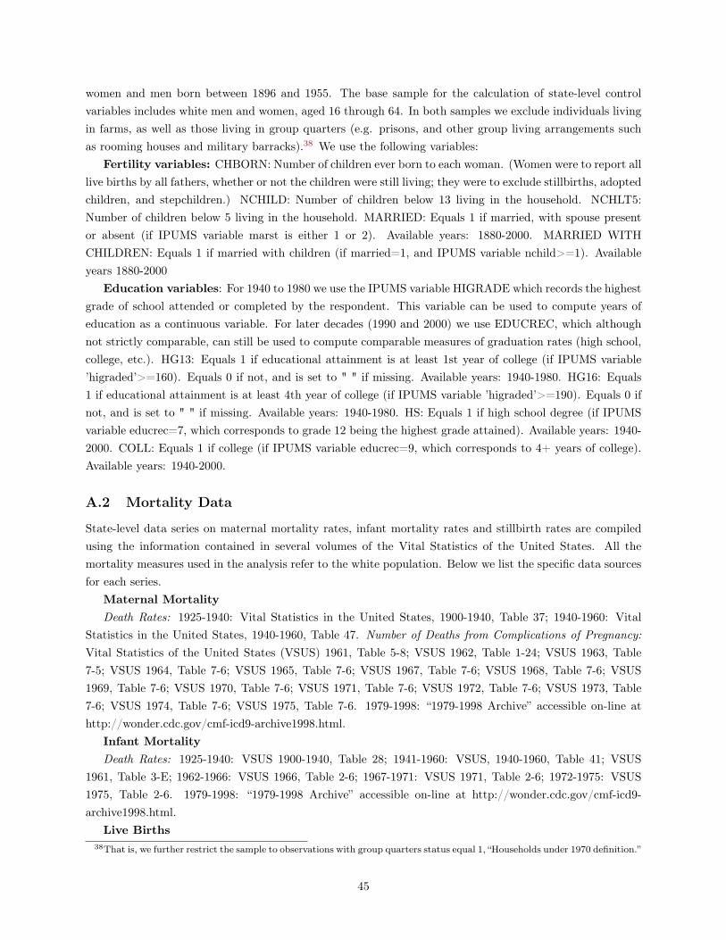
women and men born between 1896 and 1955. The base sample for the calculation of state-level controlvariables includes white men and women, aged 16 through 64. In both samples we exclude individuals livingin farms, as well as those living in group quarters (e.g. prisons, and other group living arrangements suchas rooming houses and military barracks).38 We use the following variables:

Fertility variables: CHBORN: Number of children ever born to each woman. (Women were to report alllive births by all fathers, whether or not the children were still living; they were to exclude stillbirths, adoptedchildren, and stepchildren.) NCHILD: Number of children below 13 living in the household. NCHLT5:Number of children below 5 living in the household. MARRIED: Equals 1 if married, with spouse presentor absent (if IPUMS variable marst is either 1 or 2). Available years: 1880-2000. MARRIED WITHCHILDREN: Equals 1 if married with children (if married=1, and IPUMS variable nchild>=1). Availableyears 1880-2000

Education variables: For 1940 to 1980 we use the IPUMS variable HIGRADE which records the highestgrade of school attended or completed by the respondent. This variable can be used to compute years ofeducation as a continuous variable. For later decades (1990 and 2000) we use EDUCREC, which althoughnot strictly comparable, can still be used to compute comparable measures of graduation rates (high school,college, etc.). HG13: Equals 1 if educational attainment is at least 1st year of college (if IPUMS variable’higraded’>=160). Equals 0 if not, and is set to " " if missing. Available years: 1940-1980. HG16: Equals1 if educational attainment is at least 4th year of college (if IPUMS variable ’higraded’>=190). Equals 0 ifnot, and is set to " " if missing. Available years: 1940-1980. HS: Equals 1 if high school degree (if IPUMSvariable educrec=7, which corresponds to grade 12 being the highest grade attained). Available years: 1940-2000. COLL: Equals 1 if college (if IPUMS variable educrec=9, which corresponds to 4+ years of college).Available years: 1940-2000.

A.2 Mortality Data

State-level data series on maternal mortality rates, infant mortality rates and stillbirth rates are compiledusing the information contained in several volumes of the Vital Statistics of the United States. All themortality measures used in the analysis refer to the white population. Below we list the specific data sourcesfor each series.

Maternal MortalityDeath Rates: 1925-1940: Vital Statistics in the United States, 1900-1940, Table 37; 1940-1960: Vital

Statistics in the United States, 1940-1960, Table 47. Number of Deaths from Complications of Pregnancy:Vital Statistics of the United States (VSUS) 1961, Table 5-8; VSUS 1962, Table 1-24; VSUS 1963, Table7-5; VSUS 1964, Table 7-6; VSUS 1965, Table 7-6; VSUS 1967, Table 7-6; VSUS 1968, Table 7-6; VSUS1969, Table 7-6; VSUS 1970, Table 7-6; VSUS 1971, Table 7-6; VSUS 1972, Table 7-6; VSUS 1973, Table7-6; VSUS 1974, Table 7-6; VSUS 1975, Table 7-6. 1979-1998: “1979-1998 Archive” accessible on-line athttp://wonder.cdc.gov/cmf-icd9-archive1998.html.

Infant MortalityDeath Rates: 1925-1940: VSUS 1900-1940, Table 28; 1941-1960: VSUS, 1940-1960, Table 41; VSUS

1961, Table 3-E; 1962-1966: VSUS 1966, Table 2-6; 1967-1971: VSUS 1971, Table 2-6; 1972-1975: VSUS1975, Table 2-6. 1979-1998: “1979-1998 Archive” accessible on-line at http://wonder.cdc.gov/cmf-icd9-archive1998.html.

Live Births38That is, we further restrict the sample to observations with group quarters status equal 1, “Households under 1970 definition.”

45

Birth, Stillbirth, and Infant Mortality Statistics 1931-36, Table 2; VSUS 1937-38, Table 2; VSUS 1939-41,Table 3; VSUS 1942-43, Table 9; VSUS 1944, Table 5; VSUS 1945, Table 6; VSUS 1946, Table 4; VSUS1947-48, Table 3; VSUS 1949, Table 9; VSUS 1950, Table 17; VSUS 1951-54, Table 21; VSUS 1955, Table30; VSUS 1956, Table 34; VSUS 1957, Table 33; VSUS 1959, Table 31; VSUS 1960-61, Table 2-8; VSUS1962, Table 1-36; VSUS 1963-65, Table 1-41; VSUS 1966, Table 2-1; VSUS 1967-68, Table 1-42; VSUS 1969,Table 1-72; VSUS 1970, Table 1-73; VSUS 1971-75, Table 2-1. 1979-1998: “1979-1998 Archive” accessibleon-line at http://wonder.cdc.gov/cmf-icd9-archive1998.html.

Male, Tuberculosis, Scarlet Fever Pneumonia, Influenza, Malaria Mortality RatesDeath Rates: 1900-1936 Miller (2008), available online at http://www.stanford.edu/~ngmiller/Death Rates: 1937-1940: Vital Statistics in the United States 1937-1958, Various Tables. See online

appendix for details. All data available at http://www.cdc.gov/nchs/products/vsus.htm#historical.Population1915-02 Statistical Abstract of the US Census Bureau: Chart Title Missing; 1916-02 Statistical Abstract

of the US Census Bureau: No. 23 - Population of the United States at each Census: 1790 to 1910, WithEstimates for July 1, 1916; 1917-02 Statistical Abstract of the US Census Bureau: No. 23 - Populationof the United States at each Census: 1790 to 1910, With Estimates for July 1, 1917; 1919-02 StatisticalAbstract of the US Census Bureau: No. 23 - Population of the United States at each Census: 1790 to 1910,With Estimates for July 1, 1918; 1920: 1920-02 Statistical Abstract of the US Census Bureau: No. 21 -Population of the United States at Each Census, 1790 to 1920: By States and Geographic Divisions; 1920(White): 1924-02 Statistical Abstract of the US Census Bureau: No. 10 - Population: Race, By States;VSUS 1925-1929 Mortality Statistics, Table 1 A; 1930-02 Statistical Abstract of the US Census Bureau: No.7 - Population by states: 1930, 1930 (White): 1941-02 Statistical Abstract of the US Census Bureau: No.15 - Population, by Race, by States: 1890 to 1940; 1931 - 1940: VSUS, 1900-1940; 1941 - 1960: VSUS,1940-1960; VSUS 1961, Vol. I, Natality: Table 5-4; VSUS 1962-1963, Vol. I, Natality: Table 4-5; VSUS1964. Volume I, Natality: Table 4-4; VSUS 1965. Volume I, Natality: Table 4-3; VSUS 1966. Volume I,Natality: Table 4-4; VSUS 1967-1969, Volume I, Natality: Table 4-3. 1970 - 1998: CDC Wonder CensusEstimates, 1970-1998 accessible on-line at http://wonder.cdc.gov/cmf-icd9-archive1998.html.

A.3 State Level Controls

Economic and Demographic Controls UNEMPLOYMENT RATE: We use IPUMS variable EMP-STAT to compute state level unemployment rates. SHARE OF FOREIGN BORN RESIDENTS: We useIPUMS variable BPLD that contains information on place of birth. PER-CAPITA PERSONAL INCOME:We use a state-wide measure, i.e., across all races and genders, from the Bureau of Economic Analysis (BEA),Regional Economic Accounts. This series is converted to real values using consumer price series Cc1 fromthe Millennium Statistics of the United States.

Women’s Su!rage For date of introduction of women’s su!rage, see Lott and Kenney (1999). For dateof ratification of XIX Amendment, see Mount (2007).

ACCEPTANCE YEAR: Date at which a state introduced or ratified women’s su!rage, if this precededthe date of introduction of the XIX Amendment, or the date in which the Amendment was ratified for thosestates that had no prior legislation and rejected the Amendment in 1920. There was substantial variationacross the states in the timing of the introduction or ratification of the XIX Amendment, which was approvedby Congress in 1920. Wyoming was the first State to introduce women’s su!rage in 1869, and Mississippi

46

was the last state to ratify it in 1984.

Mobilization Rates We use the state level mobilization rates constructed by Acemoglu, Autor and Lyle(2004), defined as the fraction of the 18 to 44 years old registered males in a state who were drafted forwar,39 based on published tables from the Selective Service System (1956). The average mobilization ratewas .474 with a standard deviation of .035. Mobilization rates varied substantially across states, from lessthan 42% in Georgia, the Dakotas and the Carolinas, to more than 52% in Washington, Pennsylvania, NewHampshire, Oregon, and Massachusetts. The Selective Service’s guidelines for deferments were based onmarital status, fatherhood, essential skills for civilian war production, and temporary medical disabilities,but also left considerable discretion to the local boards. Farm employment, in particular, was a major causeof deferment as maintaining food supply was considered essential to the war e!ort. The mobilization rate isalso higher in states with higher average male education and with a lower percentage of black males.

GI Bill Benefits To control for access to GI Bill educational benefits, we construct an indicator variable,IGt , reflecting whether a cohort t substantially withdrew education benefits from the GI Bill. We then interact

this variable with the percentage mobilization rate base on Acemoglu, Autor and Lyle (2004), inteded toserve as a proxie for the nuber of eligible recipients.

Based on findings in Stanley (2003) and Burns and Turner (2002), suggesting that the 1922-1928 birthcohorts displayed the largest take up of WWII GI benefits. Specifically, based on in Table 2 in Bound andTurner (2002), more than 10% of veterans achieved a bachelor’s of arts using GI benefits for these cohorts.Thus, we set IG

t = 1 for t = 1922, ...1928. We also run a specification where IGt corresponds to the percentage

of individuals who used GI benefits, in the same year, to allow for variation in intensity across cohorts.

Federal Programs for the Promotion of Maternal and Infant Health 1921-1929 Maternity andInfancy Care (Sheppard-Towner) Act: Appropriations, Payments to the States, Activities carried outunder the Act by the States, fiscal years 1921-1929: Children’s Bureau Publication N. 203 (1931). 1935Social Security Act, Title V, Part 1: Appropriations, Payments to the States, Activities carried outunder the Act by the States fiscal years 1936-1939: Children’s Bureau Publication N. 259 (1941).

Early Legal Access to Oral Contraception and Abortion Early legal access to oral contraceptionwas an outcome of increased attribution of legal rights to minors, a process which started in the late 1950swith the development of the “mature minor” doctrine. We use Bailey’s (2006) coding, described in Table 1,of “year law e!ective.” Following Bailey, we code the “year of early access to abortion” as Early access toabortion is coded as 1970 for Alaska, California, Hawaii, New York, and Washington, and 1972 for Vermontand New Jersey. All other states permitted early legal access with Roe v. Wade in 1973.

B Government Intervention in the Area of Maternal Health

The United States government enacted several programs for the promotion of maternal and infant healthstarting in the 1920s.

39Since all men in the age bracket 18-44 were registered, their mobilization rate variable represents the fraction of men inthis age range who have served. Mobilization rates for Nevada and Washington D.C. are not available (the former because itsaw large population changes during this time period).

47

1921-1929 Maternity and Infancy Care (Sheppard-Towner) Act The Sheppard-Towner Act wasfirst enacted in 1921 as a five year program. It was extended in 1926 and finally repealed in 1929.40 TheAct provided federal grants-in-aid to the states for the promotion of infant and maternal health. The mainpurpose of the Act was education, though its implementation resulted in the development of full-time unitsfor maternal and child health services, and of the first standardized training programs in this area. Asecondary objective was to expand the birth and death registration area. Although repealed in 1929, the Actset a pattern for state-Federal cooperation that would re-emerge for many other programs.41 The responseof the states to the availability of the federal funding via this legislation varied greatly. Many states didnot accept the benefits of the act for several years, though all but three states eventually accepted the actby 1928 (Skopcol, 1992, and Moehling and Thomasson, 2009). For the accepting states, the nature of theprograms financed under the act and their geographical extension also varied, as discussed in a preliminaryassessment of the submitted plans by Abbott (1922).

Appropriations: Each state was granted outright $10,000 in 1922 and $5,000 for each subsequent year.The remaining yearly apportionment of $1,000,000 was divided between the states based on population, oncondition that the states provided matching funds. A small budget was reserved also for the activities of theChildren’s Bureau, which was responsible for the review and approval of the state plans.

1935 Social Security Act Title V, Part 1, of the Social Security Act, signed into law in August 1935,provided funding for medical care of mothers and infants. The administration of Title V was modelled on theSheppard-Towner Act. The main di!erence, in addition to a doubling of appropriations, was the provisionof medical and hospital services for mothers during labor and delivery (Lesser, 1985). Participating stateswere mandated to make diagnostic services available free of charge without requirement of economic statusor legal residence. Eligibility for medical treatment could take into account family income and size, but alsothe diagnosis and the estimated cost of completed care. Means testing was typically not applied. Serviceswere provided by participating physicians and hospitals, and by public health nurses, social workers, andnutritionists. The Children’s Bureau set caps on reimbursed expenses based on the average costs for ahospital bed. Since the apportionment of funds was based on the states’ financial needs, as well as onthe number of live births, poorer states received more transfers. This system may have contributed to aconvergence in maternal health outcomes across states (Schmidt, 1973).

There were three types of yearly appropriation. A uniform yearly apportionment of $20,000 was grantedoutright to each state, whereas a yearly appropriation of $1,820,000 was divided among the states basedon the percentage of live births. An additional yearly appropriation of $980,000 was reserved for statesexperiencing financial need.

1943-1946 EMIC The Emergency Maternity and Infant Care Program (EMIC), passed into law inMarch 1943, provided funds for maternity and infant care for the wives and infants of servicemen in thefour lower pay grades. Medical, nursing, and hospital services for the prenatal period as well as deliveryand six weeks of postpartum care were provided for these families at no charge, in addition to complete carefor infants. States obtained federal funds based on need, and there was no means testing for participants.Yearly appropriations to the states were made based on the number of projected cases, with the possibility

40Skopcol (1992), Moehling and Thomasson (2009) discuss the political economy of the enactment and repeal of the Sheppard-Towner Act.

41The Sheppard-Towner Act was not the first example of federal grant-in-aid to the States, though it was the first in the areaof public health. See Skopcol (1992).

48

of deficiency appropriations. By the end of the program in 1946, approximately 1.25 million mothers and 230thousand children received care. It was the largest public medical care program undertaken in the UnitedStates up to that time (Schmidt, 1973). The program was widely recognized for the reduction in maternaland infant mortality and for the rise in the number of births attended by trained medical personnel.

1946 Hospital Survey and Construction (Hill-Burton) Act The objective of this legislation wasto attain a ratio of 4.5 beds per 1,000 population. Federal funding was provided on a grant-in-aid basis.Facilities receiving Hill-Burton were not allowed to discriminate based on race, color, national origin, orcreed, and were required to provide a "reasonable" amount of uncompensated care each year for 20 years tolocal residents who could not a!ord to pay. These restrictions limited participation in some states. In 1975,the Act was amended and became Title XVI of the Public Health Service Act.

C Theory

C.1 Basic Model

C.1.1 Proofs

Proof of Proposition 1:Totally di!erentiating the system of first order necessary conditions (1)-(2) with respect to µ for µ = µ",

and simplifying yields:

["ve!e!(b, e") + $(sb)U ""(e";µ)]%e"

%µ+ ["ve!b(b, e") + $"(sb)sU "(e";µ)]

%b

%µ= "$(sb)

%U "(e";µ)%µ

,

["vbe!(b, e") + $"(sb)sU "(e";µ)]%e"

%µ+

!"vbb(b, e") + $""(sb)s2U(e";µ)

" %b

%µ= u((1 + "e)w)" $"(sb)s

%U(e";µ)%µ

.

Solving:

%e"

%µ=" ["ve!b(b, e") + $"(sb)sU "(e";µ)]["ve!e!(b, e") + $(sb)U ""(e";µ)]

%b

%µ"

$(sb)!U !(e!;µ)!µ

["ve!e!(b, e") + $(sb)U ""(e";µ)],

#detHV

["ve!e!(b, e") + $(sb)U ""(e";µ)]

$%b

%µ

=["vbe!(b, e") + $"(sb)sU "(e";µ)]["ve!e!(b, e") + $(sb)U ""(e";µ)]

$(sb)%U "(e";µ)

%µ+ u((1 + "e)w)" $"(sb)s

%U(e";µ)%µ

.

By (3):%U "(e;µ)

%µ= "bu"(w(1 + "e))w"< 0, (13)

%U(e;µ)%µ

= "bu(w(1 + "e)) < 0. (14)

By Assumption 1, detHV > 0 and ["ve!e!(b, e") + $(sb)U ""(e";µ)] < 0. Thus, condition (6) guarantees !b!µ < 0

and !e!

!µ < 0.!Proof of Proposition 2:

49

Totally di!erentiating the system of first order necessary conditions (1)-(2) with respect to e and simpli-fying yields:

["ve!e! + $(sb)U ""(e";µ")]%e"

%e+ ["ve!b + $"(sb)sU "(e";µ")]

%b

%e= 0,

["ve!b + $"(sb)sU "(e";µ")]%e"

%e+

!"vbb + $""(sb)s2U(e";µ)

" %b

%e= µu"(w(1 + "e))"w.

Substituting for !b!e and simplifying the second equation:

%e"

%e= " ["ve!b + $"(sb)sU "(e";µ")]

["ve!e! + $(sb)U ""(e";µ")]%b

%e, (15)

%b

%e=

#detHV

["ve!e! + $(sb)U ""(e";µ")]

$$1

µu"(w(1 + "e))"w, (16)

By Assumption 1, detHV > 0 and ["ve!e!(b, e") + $(sb)U ""(e";µ)] < 0. Thus, !b!e < 0. In addition, condition

(6), equation (15) implies !e!

!e > 0.!

C.1.2 Response to a Temporary Decline in Maternal Mortality

Proposition 3 derives the response of desired fertility and investment in daughters’ human capital to atemporary decline in pregnancy-related mortality rate for the mothers’ generation.

Proposition 3 Assume the pregnancy-related mortality risk changes for the mothers’ generation. Then, byAssumption 1:

%b

%µ% 0. (17)

In addition:%e"

%µ% 0, (18)

if condition (6) holds.

Proof:Di!erentiating the system of first order necessary conditions (1)-(2) with respect to µ for given µ" and

simplifying yields:

["ve!e!(b, e") + $(sb)U ""(e";µ")]%e"

%µ+ ["ve!b(b, e") + $"(sb)sU "(e";µ")]

%b

%µ= 0,

["vbe!(b, e") + $"(sb)sU "(e";µ")]%e"

%µ+

!"vbb(b, e") + $""(sb)s2U(e";µ")

" %b

%µ= u((1 + "e)w).

Solving:

%e"

%µ=" ["ve!b(b, e") + $"(sb)sU "(e";µ")]["ve!e!(b, e") + $(sb)U ""(e";µ")]

%b

%µ,

#detHV

["ve!e!(b, e") + $(sb)U ""(e";µ")]

$%b

%µ= u((1 + "e)w).

50

Thus, by assumption 1, !b!µ < 0. In addition, condition (6) guarantees !e!

!µ < 0.!

Proposition 4 derives the sign of the response to a decline in daughters’ pregnancy-related mortality risk.

Proposition 4 Assume the pregnancy-related mortality risk changes for the daughters’ generation. Then,the optimal response of births and parental investment in human capital satisfies:

%b

%µ"% 0 , (19)

%e"

%µ"% 0, (20)

if and only if condition (6) holds.

Proof:Totally di!erentiating the first order necessary conditions (1)-(2) with respect to µ" for given µ obtains:

["ve!e!(b, e") + $(sb)U ""(e";µ")]%e"

%µ"+ ["ve!b(b, e") + $"(sb)sU "(e";µ")]

%b

%µ"= "$(sb)

%U "(e";µ")%µ"

,

["vbe!(b, e") + $"(sb)sU "(e";µ)]%e"

%µ"+

!"vbb(b, e") + $""(sb)s2U(e";µ)

" %b

%µ"= "$"(sb)s

%U(e";µ")%µ"

.

Solving:

%e"

%µ"=" ["ve!b(b, e") + $"(sb)sU "(e";µ)]["ve!e!(b, e") + $(sb)U ""(e";µ)]

%b

%µ""

$(sb)!U !(e!;µ!)!µ!

["ve!e!(b, e") + $(sb)U ""(e";µ")],

#detHV

["ve!e!(b, e") + $(sb)U ""(e";µ")]

$%b

%µ"=

["vbe!(b, e") + $"(sb)sU "(e";µ")]["ve!e!(b, e") + $(sb)U ""(e";µ")]

$(sb)%U "(e";µ")

%µ"" $"(sb)s

%U(e";µ")%µ"

.

By (13) and (14) and assumption 1, condition (6) guarantees !b!µ! < 0 and !e!

!µ! .!Proposition 4 then implies that both desired fertility and mothers’ investment in daughters’ human capital

rise when pregnancy-related mortality risk falls for daughters when condition (6) holds.

C.2 Extended Model

The model described in Section 3 can easily be extended to allow for daughters and sons. Each cohorthas a representative household, comprised by two adults of di!erent gender, indexed by f (female) and m

(male). The household decides on the number of births b, equally divided between daughters and sons andcan di!erentially select the human capital investment for daughters, e"f , and sons, e"m.

The households’ decision problem is captured by the following Bellman equation:

U(ef , em;µ) = maxe!f!0, e!

m!0, b!0

%"v(e"f , e"m, b) + (1" µb)u(w(1 + "fef )) + u(w(1 + "mem)) + $(sb)U(e"f , e"m;µ")

&.

The household’s lifetime utility depends on the human capital of the husband and the wife, who have separateutility from consumption. Returns to human capital are allowed to di!er across genders. For simplicity there

51

is no adult mortality risk for men, and daughters and sons have the same infant mortality risk.The first order necessary conditions for this choice problem are:

" vb(e"f , e"m, b)" µu(w(1 + "fef )) + $"(sb)sU(e"f , e"m;µ") = 0, (21)

" vej (e"f , e"m, b) + $(sb)Uej (e

"f , e"m;µ") % 0, (22)

with equality for e"j > 0 for j = f, m,

Uef (ef , em;µ) = (1" µb)u"(w(1 + "fef ))w"f ,

Uem(ef , em;µ) = u"(w(1 + "mem))w"m.

The envelope conditions clearly suggest that the optimal human capital investment should be lower for girlsif pregnancy related mortality is di!erent from 0.

As for the basic model, we will impose joint concavity of household welfare in the choice vector {b, e"f , e"m}.we will impose the following assumption:

Assumption 2 Let: V (e"f , e"j , b;µ, µ") := "v(e"f , e"m, b)+$(sb)U(e"f , e"m;µ") is strictly concave in {b, e"f , e"m}.

Assumption 2 implies that the Hessian of V , denoted with HV (e"f , e"j , b;µ, µ"), is negative definite.We now derive the e!ect of a permanent decline in µ from the parents’ cohort.

Proposition 5 Assume that pregnancy-related mortality risk is the same for mothers and daughters, so thatµ = µ", and that it changes permanently starting with the mother’s generation. Then, under Assuption 2,the optimal response of births and parental investment in human capital satisfies:

%b

%µ% 0, (23)

%e"f%µ

% 0, (24)

if and only if: '"vbe!

j(b, e") + $"(sb)sUe!

j(e";µ")

(> 0, (25)

for j = f, m and: '"ve!

me!f(b, e") + $(sb)Ue!

me!f(e";µ")

(# 0. (26)

Proof:Totally di!erentiating the system of first order necessary conditions (21)-(22) with respect to µ for µ = µ"

at an interior solution, and simplifying yields:

)

**+

!b!µ!e!

f

!µ!e!

m!µ

,

--. = H$1V

)

**+

"$"(sb)s!U(e!f ,e!

m;µ)

!µ + u(w(1 + "fef ))

"$(sb)!Ue!

f(e!

f ,e!m;µ)

!µ

0

,

--. .

Assumption 2 implies that HV is negative definite, thus, !b!µ < 0 if:

!"vbe!

m(b, e") + $"(sb)sUe!

m(e";µ")

" '"ve!

me!f(b, e") + $(sb)Ue!

me!f(e";µ")

(>

52

'"vbe!

f(b, e") + $"(sb)sUe!

f(e";µ")

( !"ve!

me!m

(b, e") + $(sb)Ue!me!

m(e";µ")

".

This restriction is satisfied under conditions (25) and (26).Similarly, by assumption 2, !e!

f

!µ < 0 if:

'"ve!

f e!m

(b, e") + $(sb)Ue!f e!

m(e";µ")

( !"vbe!

m(b, e") + $"(sb)sUe!

m(e";µ")

"

>'"vbe!

f(b, e") + $"(sb)sUe!

f(e";µ")

( !"ve!

me!m

(b, e") + $(sb)Ue!me!

m(e";µ")

".

Conditions (25) and (26) guarantee this restriction will hold. !Proposition 6 shows that desired fertility is decreasing in the mother’s endowment of human capital.

Proposition 6 Assumption (2) implies:

%b(ef , em;µ)%ef

% 0. (27)

Proof:Totally di!erentiating the system of first order necessary conditions (21)-(22) with respect toef at an

interior equilibrium obtains:

)

**+

!b!ef

!e!f

!ef

!e!m

!ef

,

--. = H$1V

)

*+µu"(w(1 + "fef ))w"f

00

,

-. .

Thus, by Assumption 2, !b!ef

< 0. !

53

D Additional Empirical Results

Table 15: Fertility_ Sulfa Mortalities as Instrument

Specification

Fertility Outcome CHBORN CHBORN CHBORN NCHILD NCHILD NCHILD NCHLT5 NCHLT5 NCHLT5

Sample Married All

Married with

children Married All

Married with

children Married All

Married with

childrenAge 35-44 35-44 35-44 35-44 35-44 35-44 23-32 23-32 23-32

Constant 3.8114 3.8 4.8701 1.6424 1.5313 1.9599 0.9457 0.8426 1.0647

t-stat 16.6202 17.6988 14.9979 13.2628 13.2984 16.7524 12.3888 12.6972 11.2666SulfaMRpre

s*It (2) (3) 0.0158 0.0147 0.0077 0.0084 0.0082 0.0072 0.0027 0.0032 0.0021

t-stat 10.7525 10.6951 3.6999 10.5764 11.1904 9.6575 5.5588 7.4853 3.4625IMRref

st (3) -0.0259 -0.0275 -0.0361 0.0026 0.0023 0.0056 -0.0044 -0.005 -0.002

t-stat -9.1813 -10.4366 -9.0519 1.7197 1.6463 3.9027 -4.6435 -6.1578 -1.6957

Adj R-squared 0.4234 0.4706 0.2179 0.2648 0.3305 0.1941 0.2597 0.3299 0.1879

R-squared 0.4444 0.4899 0.2465 0.2916 0.3549 0.2235 0.2867 0.3544 0.2175

Model p-value 0 0 0 0 0 0 0 0 0

(1) Baseline specification. All regressions include state and cohort effects. Control group: 1913-1920. Treated group: 1921-1940.

(3) The reference mortality rate for each disease is the average of the mortality rate for that disease in the state at age 15-20. (4) Reference infant mortality is the average infant mortality in the state at age 15-20.

IV

Regression Results (1)

(2) The instrument for reference MMR in each state is the average reference mortality rate for diseases treatable with sulfa drugs for the control cohorts in each state. The diseases tretable with sulfa drugs are pneumonia and influenza and scarlet fever.

54

Tab

le16

:Fa

lsifi

cation

Exe

rcis

e

Incl

ud

ed

Bir

th C

oh

ort

s1

90

5-1

91

51

91

0-1

91

51

92

1-1

94

0R

efe

ren

ce M

MR

Ag

e 1

5-2

8 (

2)

Ag

e 1

5-2

3 (

2)

Ag

e 1

5-2

8 (

3)

Sta

tist

ics

mean

(MM

R)

56.0

2759

.255

29.

1082

std

(MM

R)

8.24

28.

7857

1.94

38

Fert

ilit

y O

utc

om

eC

HB

OR

NC

HB

OR

NC

HB

OR

NC

HB

OR

NC

HB

OR

NC

HB

OR

NC

HB

OR

NC

HB

OR

NC

HB

OR

NA

ge

35

-44

35

-44

35

-44

35

-44

35

-44

35

-44

35

-44

35

-44

35

-44

Sam

ple

All

Marr

ied

Marr

ied

w

ith

ch

ild

ren

All

Marr

ied

Marr

ied

w

ith

ch

ild

ren

All

Marr

ied

Marr

ied

w

ith

ch

ild

ren

Con

stan

t8.

1464

32.9

638

19.5

245

28.7

379

30.4

389

21.3

412

34.9

224

42.9

063

-68.

3318

t-st

at0.

5641

2.17

341.

0751

1.25

061.

2801

0.78

815.

0049

5.76

24-2

.842

5M

MR

ref st

0.

0075

0.00

570.

0079

-0.0

04-0

.000

40.

0053

-0.0

46

-0.0

46

30.

0001

t-st

at1.

7545

1.26

71.

4702

-0.6

972

-0.0

702

0.77

88-1

1.39

03-1

0.72

750.

0071

IMR

ref st

(4

)-0

.006

6-0

.011

8-0

.011

40.

0001

-0.0

041

-0.0

121

0.01

750.

0185

0.00

48t-

stat

-1.3

558

-2.3

295

-1.8

663

0.01

74-0

.600

9-1

.572

4.67

4.60

580.

3679

Ad

j R

-sq

uare

d0.

5676

0.56

160.

4677

0.60

680.

6017

0.53

270.

6649

0.53

710.

054

Incl

ud

ed

Bir

th C

oh

ort

s1

91

0-1

91

71

91

8-1

92

51

93

3-1

95

0R

efe

ren

ce M

MR

Ag

e 5

-23

(2

)A

ge 5

-15

(2

)A

ge 5

-23

(3

)

Sta

tist

ics

mean

(MM

R)

59.5

396

56.7

425

6.18

9st

d(M

MR

)8.

5992

8.33

141.

3483

Ed

uca

tio

nal

Att

ain

men

t at

ag

e 2

3-3

2H

SC

OLL

HS

CO

LLH

SC

OLL

HS

CO

LLH

SC

OLL

HS

CO

LLS

am

ple

All

All

Marr

ied

Marr

ied

All

All

Marr

ied

Marr

ied

All

All

Marr

ied

Marr

ied

Con

stan

t0.

1639

0.04

140.

1391

0.03

150.

0759

0.03

120.

0814

0.02

830.

3765

0.14

570.

3942

0.14

29t-

stat

7.84

393.

4186

5.60

762.

201

5.56

593.

4826

5.64

643.

5521

26.8

056

9.36

0224

.335

27.

7848

MM

Rre

f st *

Fg

(4

)-0

.00

96

0.00

1-0

.00

79

0.0

02

2-0

.00

20

-0.0

01

7-0

.000

1-0

.000

8-0

.00

95

-0.0

01

5-0

.00

91

t-st

at-9

.761

71.

7432

-6.7

639

3.21

4-4

.860

1-0

.136

7-3

.873

5-0

.292

2-1

.627

6-1

7.20

6-2

.539

2-1

3.94

21A

dj

R-s

qu

are

d0.

7242

0.43

870.

6501

0.27

320.

4752

0.21

910.

4401

0.19

270.

5537

0.55

990.

4894

0.46

3

(1)

Bas

elin

e sp

ecifi

cation

. All

regr

essi

ons

incl

ude

stat

e an

d co

hort

effec

ts.

(3)

Rob

ustn

ess

exer

cise

. O

rigi

nal t

reat

ed c

ohor

ts,

refe

renc

e M

MR a

s in

mai

n fa

lsifi

cation

exe

rcis

e.(4

) Ref

eren

ce in

fant

mor

talit

y is

the

ave

rage

infa

nt m

orta

lity

in t

he s

tate

at

age

15-2

0.

(5)

Spe

cific

atio

n in

clud

es ful

ly in

tera

cted

sta

te,

coho

rt a

nd g

ende

r ef

fect

s.

(2)

Ref

eren

ce M

MR is

the

ave

rage

mor

talit

y ra

te in

the

sta

te in

a g

iven

age

ran

ge for

eac

h co

hort

. Sin

ce t

he e

arlie

st y

ear

whe

re M

MR is

ava

ilabl

e fo

r al

l sta

tes

is 1

933,

we

mus

t ex

tend

the

age

for

ref

eren

ce M

MR

rela

tive

to

the

base

line

spec

ifica

tion

, fo

r w

hich

the

age

ran

ge is

15-

20 for

fer

tilit

y an

d 5=

10 for

edu

cation

.

Co

ntr

ol

Gro

up

IC

on

tro

l G

rou

p I

ITre

atm

en

t G

rou

p

Fert

ilit

y (1

)

Ed

uca

tio

n (

5)

Co

ntr

ol

Gro

up

IC

on

tro

l G

rou

p I

ITre

atm

en

t G

rou

p

55