Embed Size (px)
Citation preview

IntroductionSpending-Restricted Outcome
Approximation Algorithm
Nash Welfare, Market Equilibrium,and Stable Polynomials
STOC 2019 tutorial23 June 2019
Nima Anari Stanford UniversityJugal Garg University of Illinois at Urbana ChampaignVasilis Gkatzelis Drexel University
Nima Anari, Jugal Garg, and Vasilis Gkatzelis Nash Welfare, Market Equilibrium, and Stable Polynomials

IntroductionSpending-Restricted Outcome
Approximation Algorithm
Resource AllocationNash Social WelfareApproximation Guarantee
Overview
First Section (9-10am)“Approximating the Nash Social Welfare with Indivisible Items”Vasilis Gkatzelis
Second Section (10-11am)“NSW Beyond Symmetric Agents with Additive Valuations”Jugal Garg
Coffee Break (11-11:20pm)
Third Section (11:20-12:20pm)“Nash Social Welfare and Stable Polynomials”Nima Anari
Nima Anari, Jugal Garg, and Vasilis Gkatzelis Nash Welfare, Market Equilibrium, and Stable Polynomials

IntroductionSpending-Restricted Outcome
Approximation Algorithm
Resource AllocationNash Social WelfareApproximation Guarantee
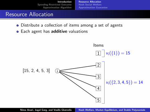
Resource Allocation
Distribute a collection of items among a set of agents
Each agent has additive valuations
i
5
4
3
2
1
[vi1, vi2, vi3, vi4, vi5][15, 2, 4, 5, 3]
vi ({1}) = 15
vi ({2}) = 2
vi ({2, 3}) = 6
vi ({2, 3, 4}) = 11
vi ({2, 3, 4, 5}) = 14
Items
Nima Anari, Jugal Garg, and Vasilis Gkatzelis Nash Welfare, Market Equilibrium, and Stable Polynomials

IntroductionSpending-Restricted Outcome
Approximation Algorithm
Resource AllocationNash Social WelfareApproximation Guarantee
Resource Allocation
Distribute a collection of items among a set of agents
Each agent has additive valuations
i
5
4
3
2
1
[vi1, vi2, vi3, vi4, vi5][15, 2, 4, 5, 3]
vi ({1}) = 15
vi ({2}) = 2
vi ({2, 3}) = 6
vi ({2, 3, 4}) = 11
vi ({2, 3, 4, 5}) = 14
Items
Nima Anari, Jugal Garg, and Vasilis Gkatzelis Nash Welfare, Market Equilibrium, and Stable Polynomials

IntroductionSpending-Restricted Outcome
Approximation Algorithm
Resource AllocationNash Social WelfareApproximation Guarantee
Setting
Set N of n agents and set M of m indivisible items
For each agent i and item j : xij ∈ {0, 1}For each agent i : vi(x) =
∑j∈M xijvij
4
3
2
1
5
4
3
2
1
[3,2,1,1,1]
[15,0,1,1,1]
[15,2,0,0,0]
[1,0,0,0,0]
Agents Items
Nima Anari, Jugal Garg, and Vasilis Gkatzelis Nash Welfare, Market Equilibrium, and Stable Polynomials

IntroductionSpending-Restricted Outcome
Approximation Algorithm
Resource AllocationNash Social WelfareApproximation Guarantee
Utilitarian Social Welfare
Maximize the utilitarian social welfare: maxx
∑i∈N
vi (x)
2
1
8
7
6
5
4
3
2
1
[1,1,1,1,7,7,7,7]
[1,1,1,1,1,1,1,1]
Agents Items
Nima Anari, Jugal Garg, and Vasilis Gkatzelis Nash Welfare, Market Equilibrium, and Stable Polynomials

IntroductionSpending-Restricted Outcome
Approximation Algorithm
Resource AllocationNash Social WelfareApproximation Guarantee
Egalitarian Social Welfare [BS’06,AS’10,F’08,...]
Maximize the egalitarian social welfare: maxx
{mini∈N
vi (x)
}
2
1
8
7
6
5
4
3
2
1
[1,1,1,1,7,7,7,7]
[1,1,1,1,1,1,1,1]
Agents Items
Nima Anari, Jugal Garg, and Vasilis Gkatzelis Nash Welfare, Market Equilibrium, and Stable Polynomials

IntroductionSpending-Restricted Outcome
Approximation Algorithm
Resource AllocationNash Social WelfareApproximation Guarantee
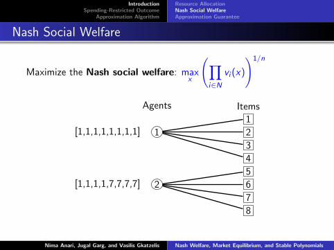
Nash Social Welfare
Maximize the Nash social welfare: maxx
(∏i∈N
vi (x)
)1/n
2
1
8
7
6
5
4
3
2
1
[1,1,1,1,7,7,7,7]
[1,1,1,1,1,1,1,1]
Agents Items
Nima Anari, Jugal Garg, and Vasilis Gkatzelis Nash Welfare, Market Equilibrium, and Stable Polynomials

IntroductionSpending-Restricted Outcome
Approximation Algorithm
Resource AllocationNash Social WelfareApproximation Guarantee
Nash Social Welfare
Maximize the Nash social welfare: maxx
(∏i∈N
vi (x)
)1/n
2
1
8
7
6
5
4
3
2
1
[1,1,1,1,7,7,7,7]
[1,1,1,1,1,1,1,1]
Agents Items
Nima Anari, Jugal Garg, and Vasilis Gkatzelis Nash Welfare, Market Equilibrium, and Stable Polynomials

IntroductionSpending-Restricted Outcome
Approximation Algorithm
Resource AllocationNash Social WelfareApproximation Guarantee
Nash Social Welfare
The Nash SW objective satisfies highly desired properties:
Scale-independenceUsing v ′
ij = αivij for any αi > 0 does not affect the outcomeAvoids interpersonal comparability of individual’s preferences
Strikes a balance between fairness and efficiency
maxx
(1
n
∑i
[vi (x)]p
)1/p
Discovered by different communities:
Nash Bargaining [Nash ’50]
Proportional Fairness [Kelly ’97]
Competitive Equilibrium from Equal Incomes [Varian ’74]
Nima Anari, Jugal Garg, and Vasilis Gkatzelis Nash Welfare, Market Equilibrium, and Stable Polynomials

IntroductionSpending-Restricted Outcome
Approximation Algorithm
Resource AllocationNash Social WelfareApproximation Guarantee
Approximation Guarantee
Let x∗ be the integral allocation maximizing the Nash SW
Goal: Design algorithm computing an integral allocation x :(∏i∈N
vi (x)
)1/n
≥ 1
ρ·
(∏i∈N
vi (x∗)
)1/n
The first known algorithm achieved ρ ∈ Θ(m) [NR’14]
The problem is NP-hard even for two identical agents
In fact, this problem is APX-hard [L’15]
Theorem (CG’15, CDGJMVY’17)
There exists a poly-time algorithm that achieves ρ = 2
Nima Anari, Jugal Garg, and Vasilis Gkatzelis Nash Welfare, Market Equilibrium, and Stable Polynomials

IntroductionSpending-Restricted Outcome
Approximation Algorithm
Program FormulationMarket EquilibriumSpending-Restricted Outcome
Program Formulation
This problem can be expressed as an integer program (IP):
maximize:
(∏i∈N
ui
)1/n
subject to:∑j∈M
xijvij = ui , ∀i ∈ N
∑i∈N
xij ≤ 1, ∀j ∈ M
xij ∈ {0, 1}, ∀i ∈ N, j ∈ M
Observation
The integrality gap of the integer program IP is unbounded!
Nima Anari, Jugal Garg, and Vasilis Gkatzelis Nash Welfare, Market Equilibrium, and Stable Polynomials

IntroductionSpending-Restricted Outcome
Approximation Algorithm
Program FormulationMarket EquilibriumSpending-Restricted Outcome
Program Formulation
This problem can be expressed as an integer program (IP):
maximize:∑i∈N
log ui
subject to:∑j∈M
xijvij = ui , ∀i ∈ N
∑i∈N
xij ≤ 1, ∀j ∈ M
xij ≥ 0, ∀i ∈ N, j ∈ M
Observation
The integrality gap of the integer program IP is unbounded!
Nima Anari, Jugal Garg, and Vasilis Gkatzelis Nash Welfare, Market Equilibrium, and Stable Polynomials

IntroductionSpending-Restricted Outcome
Approximation Algorithm
Program FormulationMarket EquilibriumSpending-Restricted Outcome
Program Formulation
The relaxation of IP is equivalent to the Eisenberg-Gale program:
maximize:∑i∈N
log ui
subject to:∑j∈M
xijvij = ui , ∀i ∈ N
∑i∈N
xij ≤ 1, ∀j ∈ M
xij ≥ 0, ∀i ∈ N, j ∈ M
Observation
The integrality gap of the integer program IP is unbounded!
Nima Anari, Jugal Garg, and Vasilis Gkatzelis Nash Welfare, Market Equilibrium, and Stable Polynomials

IntroductionSpending-Restricted Outcome
Approximation Algorithm
Program FormulationMarket EquilibriumSpending-Restricted Outcome
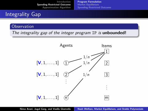
Integrality Gap
Observation
The integrality gap of the integer program IP is unbounded!
n
...
2
1
m
...
3
2
1
[V, 1, . . . , 1]
[V, 1, . . . , 1]
[V, 1, . . . , 1]
Agents Items
1/n
1/n
1/n
Nima Anari, Jugal Garg, and Vasilis Gkatzelis Nash Welfare, Market Equilibrium, and Stable Polynomials

IntroductionSpending-Restricted Outcome
Approximation Algorithm
Program FormulationMarket EquilibriumSpending-Restricted Outcome
Integrality Gap
Observation
The integrality gap of the integer program IP is unbounded!
n
...
2
1
m
...
3
2
1
[V, 1, . . . , 1]
[V, 1, . . . , 1]
[V, 1, . . . , 1]
Agents Items
1/n
1/n
1/n
Nima Anari, Jugal Garg, and Vasilis Gkatzelis Nash Welfare, Market Equilibrium, and Stable Polynomials

IntroductionSpending-Restricted Outcome
Approximation Algorithm
Program FormulationMarket EquilibriumSpending-Restricted Outcome
Integrality Gap
Observation
The integrality gap of the integer program IP is unbounded!
n
...
2
1
m
...
3
2
1
[V, 1, . . . , 1]
[V, 1, . . . , 1]
[V, 1, . . . , 1]
Agents Items
Nima Anari, Jugal Garg, and Vasilis Gkatzelis Nash Welfare, Market Equilibrium, and Stable Polynomials

IntroductionSpending-Restricted Outcome
Approximation Algorithm
Program FormulationMarket EquilibriumSpending-Restricted Outcome
Market Equilibrium Interpretation
Each agent is allocated a budget of $1
4
3
2
1
5
4
3
2
1
[3,2,1,1,1]
[15,0,1,1,1]
[15,2,0,0,0]
[15,0,0,0,0]
$0.2
$0.2
$0.2
$0.4
$3
Agents Items
$1
$1
$1
$0.4
$0.2
$0.2
$0.2
Nima Anari, Jugal Garg, and Vasilis Gkatzelis Nash Welfare, Market Equilibrium, and Stable Polynomials

IntroductionSpending-Restricted Outcome
Approximation Algorithm
Program FormulationMarket EquilibriumSpending-Restricted Outcome
Market Equilibrium Interpretation
Each agent is allocated a budget of $1 and item j has price pj
4
3
2
1
5
4
3
2
1
[3,2,1,1,1]
[15,0,1,1,1]
[15,2,0,0,0]
[15,0,0,0,0]
$0.2
$0.2
$0.2
$0.4
$3
Agents Items
$1
$1
$1
$0.4
$0.2
$0.2
$0.2
Nima Anari, Jugal Garg, and Vasilis Gkatzelis Nash Welfare, Market Equilibrium, and Stable Polynomials

IntroductionSpending-Restricted Outcome
Approximation Algorithm
Program FormulationMarket EquilibriumSpending-Restricted Outcome
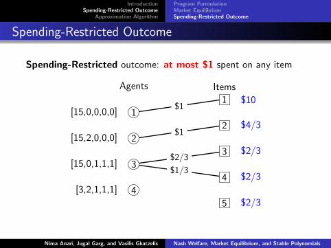
Spending-Restricted Outcome
Spending-Restricted outcome: at most $1 spent on any item
4
3
2
1
5
4
3
2
1
[3,2,1,1,1]
[15,0,1,1,1]
[15,2,0,0,0]
[15,0,0,0,0]
$0.2
$0.2
$0.2
$0.4
$3
Agents Items
$1
$1
$1
$0.4
$0.2
$0.2
$0.2
Nima Anari, Jugal Garg, and Vasilis Gkatzelis Nash Welfare, Market Equilibrium, and Stable Polynomials

IntroductionSpending-Restricted Outcome
Approximation Algorithm
Program FormulationMarket EquilibriumSpending-Restricted Outcome
Spending-Restricted Outcome
Spending-Restricted outcome: at most $1 spent on any item
4
3
2
1
5
4
3
2
1
[3,2,1,1,1]
[15,0,1,1,1]
[15,2,0,0,0]
[15,0,0,0,0]
$2/3
$2/3
$2/3
$4/3
$10
Agents Items
$1
$1
$2/3
$1/3
$2/3
$1/3
Nima Anari, Jugal Garg, and Vasilis Gkatzelis Nash Welfare, Market Equilibrium, and Stable Polynomials

IntroductionSpending-Restricted Outcome
Approximation Algorithm
Computing the SR outcomeUpper BoundSRR Algorithm
Main Technical Contributions
The main technical contributions in the rest of the tutorial are:
1 SR outcome is computable in poly-time
2 SR outcome implies a better upper bound for OPT
3 SR outcome reveals useful information for rounding
Nima Anari, Jugal Garg, and Vasilis Gkatzelis Nash Welfare, Market Equilibrium, and Stable Polynomials

IntroductionSpending-Restricted Outcome
Approximation Algorithm
Computing the SR outcomeUpper BoundSRR Algorithm
1. Computing the SR outcome [CG’15]
Expressing the SR outcome via a convex program is not trivial:
Spending constraint combines primal and dual variables
Computed via complicated primal-dual algorithm in [CG’15]
maximize:∑i∈N
log ui
subject to:∑j∈M
xijvij = ui , ∀i ∈ N
∑i∈N
xij = 1, ∀j ∈ M
xij ≥ 0, ∀i ∈ N, j ∈ M
Nima Anari, Jugal Garg, and Vasilis Gkatzelis Nash Welfare, Market Equilibrium, and Stable Polynomials

IntroductionSpending-Restricted Outcome
Approximation Algorithm
Computing the SR outcomeUpper BoundSRR Algorithm
1. Computing the SR outcome [CG’15]
Expressing the SR outcome via a convex program is not trivial:
Spending constraint combines primal and dual variables
Computed via complicated primal-dual algorithm in [CG’15]
maximize:∑i∈N
log ui
subject to:∑j∈M
xijvij = ui , ∀i ∈ N
∑i∈N
xijpj = min{1,pj} ∀j ∈ M
xij ≥ 0, ∀i ∈ N, j ∈ M
Nima Anari, Jugal Garg, and Vasilis Gkatzelis Nash Welfare, Market Equilibrium, and Stable Polynomials

IntroductionSpending-Restricted Outcome
Approximation Algorithm
Computing the SR outcomeUpper BoundSRR Algorithm
1. Computing the SR outcome [CDGJMVY’17]
An alternative “integer” program for the optimal NSW:
Let bij be the amount that agent i spends on item j
Let qj be the total amount spent on item j across all agents
max (∏
i ui )1/n s.t.
∀i , ui =∑
j xijvij
∀j ,∑
i xij = 1
∀i , j , xij ∈ {0, 1}.
max
(∏i
∏j v
bijij∏
j qqjj
)1/n
s.t.
∀j ,∑
i bij = qj
∀i ,∑
j bij = 1
∀i , j , qj ≤ 1, bij ∈ {0, qj}
Nima Anari, Jugal Garg, and Vasilis Gkatzelis Nash Welfare, Market Equilibrium, and Stable Polynomials

IntroductionSpending-Restricted Outcome
Approximation Algorithm
Computing the SR outcomeUpper BoundSRR Algorithm
1. Computing the SR outcome [CDGJMVY’17]
Solving the relaxation of this program yields the SR outcome!
Let bij be the amount that agent i spends on item j
Let qj be the total amount spent on item j across all agents
max (∏
i ui )1/n s.t.
∀i , ui =∑
j xijvij
∀j ,∑
i xij = 1
∀i , j , xij ∈ {0, 1}.
max
(∏i
∏j v
bijij∏
j qqjj
)1/n
s.t.
∀j ,∑
i bij = qj
∀i ,∑
j bij = 1
∀i , j , qj ≤ 1, bij ∈ [0, qj ]
Nima Anari, Jugal Garg, and Vasilis Gkatzelis Nash Welfare, Market Equilibrium, and Stable Polynomials

IntroductionSpending-Restricted Outcome
Approximation Algorithm
Computing the SR outcomeUpper BoundSRR Algorithm
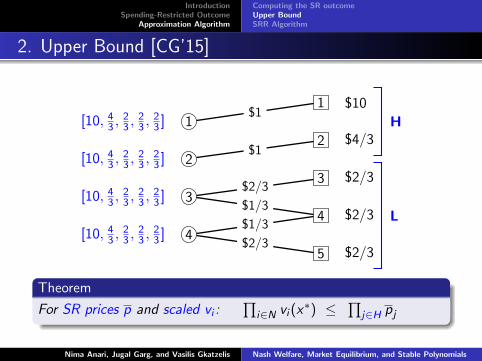
2. Upper Bound [CG’15]
4
3
2
1
5
4
3
2
1
[3,2,1,1,1]
[15,0,1,1,1]
[15,2,0,0,0]
[15,0,0,0,0]
[2, 43 ,23 ,
23 ,
23 ]
[10, 0, 23 ,23 ,
23 ]
[10, 43 , 0, 0, 0]
[10, 0, 0, 0, 0]
$2/3
$2/3
$2/3
$4/3
$10
H
L
$1
$1
$2/3
$1/3
$1/3
$2/3
Theorem
For SR prices p and scaled vi :∏
i∈N vi (x∗) ≤
∏j∈H pj
Nima Anari, Jugal Garg, and Vasilis Gkatzelis Nash Welfare, Market Equilibrium, and Stable Polynomials

IntroductionSpending-Restricted Outcome
Approximation Algorithm
Computing the SR outcomeUpper BoundSRR Algorithm
2. Upper Bound [CG’15]
4
3
2
1
5
4
3
2
1
[3,2,1,1,1]
[15,0,1,1,1]
[15,2,0,0,0]
[15,0,0,0,0]
[2, 43 ,23 ,
23 ,
23 ]
[10, 0, 23 ,23 ,
23 ]
[10, 43 , 0, 0, 0]
[10, 0, 0, 0, 0]
$2/3
$2/3
$2/3
$4/3
$10
H
L
$1
$1
$2/3
$1/3
$1/3
$2/3
Theorem
For SR prices p and scaled vi :∏
i∈N vi (x∗) ≤
∏j∈H pj
Nima Anari, Jugal Garg, and Vasilis Gkatzelis Nash Welfare, Market Equilibrium, and Stable Polynomials
IntroductionSpending-Restricted Outcome
Approximation Algorithm
Computing the SR outcomeUpper BoundSRR Algorithm
2. Upper Bound [CG’15]
4
3
2
1
5
4
3
2
1
[10, 43 ,23 ,
23 ,
23 ]
[10, 43 ,23 ,
23 ,
23 ]
[10, 43 ,23 ,
23 ,
23 ]
[10, 43 ,23 ,
23 ,
23 ]
$2/3
$2/3
$2/3
$4/3
$10
H
L
$1
$1
$2/3
$1/3
$1/3
$2/3
Theorem
For SR prices p and scaled vi :∏
i∈N vi (x∗) ≤
∏j∈H pj
Nima Anari, Jugal Garg, and Vasilis Gkatzelis Nash Welfare, Market Equilibrium, and Stable Polynomials

IntroductionSpending-Restricted Outcome
Approximation Algorithm
Computing the SR outcomeUpper BoundSRR Algorithm
2. Upper Bound [CDGJMVY’17]
New program’s optimal value is equal to previous upper bound!
Normalizing so that vij = pj when bij > 0 gives∏i
∏j v
bijij∏
j qqjj
=
∏j p
∑i bij
j∏j q
qjj
=∏j
(pjqj
)qj
Then, observing that qj = pj if j ∈ L, and qj = 1 if j ∈ H:
∏j
(pjqj
)qj
=∏j∈L
1qj ·∏j∈H
pj =∏j∈H
pj
Nima Anari, Jugal Garg, and Vasilis Gkatzelis Nash Welfare, Market Equilibrium, and Stable Polynomials

IntroductionSpending-Restricted Outcome
Approximation Algorithm
Computing the SR outcomeUpper BoundSRR Algorithm
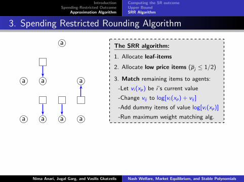
3. Spending Restricted Rounding Algorithm
a
a a a
a a a a
$1.3 $0.3
$1.5 $0.8 $0.9
The SRR algorithm:
1. Allocate leaf-items
2. Allocate low price items (pj ≤ 1/2)
3. Match remaining items to agents:
-Let vi (xp) be i ’s current value
-Change vij to log[vi (xp) + vij ]
-Add dummy items of value log[vi (xp)]
-Run maximum weight matching alg.
Theorem
The allocation x that the SRR algorithm computes satisfies:(∏i∈N
vi (x∗)
)1/n
≤ 2 ·
(∏i∈N
vi (x)
)1/n
Nima Anari, Jugal Garg, and Vasilis Gkatzelis Nash Welfare, Market Equilibrium, and Stable Polynomials

IntroductionSpending-Restricted Outcome
Approximation Algorithm
Computing the SR outcomeUpper BoundSRR Algorithm
3. Spending Restricted Rounding Algorithm
a
a a a
a a a a
$1.3 $0.3
$1.5 $0.8 $0.9
The SRR algorithm:
1. Allocate leaf-items
2. Allocate low price items (pj ≤ 1/2)
3. Match remaining items to agents:
-Let vi (xp) be i ’s current value
-Change vij to log[vi (xp) + vij ]
-Add dummy items of value log[vi (xp)]
-Run maximum weight matching alg.
Theorem
The allocation x that the SRR algorithm computes satisfies:(∏i∈N
vi (x∗)
)1/n
≤ 2 ·
(∏i∈N
vi (x)
)1/n
Nima Anari, Jugal Garg, and Vasilis Gkatzelis Nash Welfare, Market Equilibrium, and Stable Polynomials

IntroductionSpending-Restricted Outcome
Approximation Algorithm
Computing the SR outcomeUpper BoundSRR Algorithm
Overview
First Section (9-10am)“Approximating the Nash Social Welfare with Indivisible Items”Vasilis Gkatzelis
Second Section (10-11am)“NSW Beyond Symmetric Agents with Additive Valuations”Jugal Garg
Coffee Break (11-11:20pm)
Third Section (11:20-12:20pm)“Nash Social Welfare and Stable Polynomials”Nima Anari
Nima Anari, Jugal Garg, and Vasilis Gkatzelis Nash Welfare, Market Equilibrium, and Stable Polynomials

IntroductionSpending-Restricted Outcome
Approximation Algorithm
Computing the SR outcomeUpper BoundSRR Algorithm
Thank you!
THANK YOU!
Nima Anari, Jugal Garg, and Vasilis Gkatzelis Nash Welfare, Market Equilibrium, and Stable Polynomials