NASA WATER VAPOR PROJECT – MEaSUREs

(NVAP-M)

ALGORITHM THEORETICAL BASIS DOCUMENT

Version 2

Thomas Vonder Haar, PI

John Forsythe

Janice Bytheway

Science and Technology Corporation

METSAT Division

10 Basil Sawyer Drive

Hampton, VA 23666-1393

Vonderhaar@stcnet.com

February, 2013

2

Table of Contents

1. Introduction .............................................................................................................................................. 3

1.1 Overview and Background Information ............................................................................................ 3

1.1 Science Applications .......................................................................................................................... 3

1.2 Need for Reanalysis and Extension ................................................................................................... 4

1.3 NVAP-MEaSUREs Design Philosophy ................................................................................................. 6

2. Input Dataset Descriptions........................................................................................................................ 7

2.1 Special Sensor Microwave Imager (SSM/I) ........................................................................................ 7

2.2 High Resolution Infrared Sounder (HIRS) .......................................................................................... 9

2.3 Radiosonde ........................................................................................................................................ 9

2.4 Atmospheric Infrared Sounder (AIRS) ............................................................................................. 11

2.5 Global Positioning System (GPS) ....................................................................................................... 12

2.6 Ancillary Data .................................................................................................................................... 13

2.6.1 Modern Era Retrospective Analysis for Research Applications (MERRA) .................................. 13

2.6.2 AIRS Climatology ........................................................................................................................ 14

2.6.3 Sea Surface Temperature ........................................................................................................... 15

3. Retrieval Algorithms................................................................................................................................ 15

3.1 Microwave Retrieval Algorithm ........................................................................................................ 15

3.2 Infrared Retrieval Algorithm ............................................................................................................. 19

4. Merging of Water Vapor Data into a Single Product .............................................................................. 21

5. References .............................................................................................................................................. 22

Appendix A: Dataset Description ................................................................................................................ 26

A.1 Naming Convention .......................................................................................................................... 26

A.2 Product List ....................................................................................................................................... 26

Appendix B: Acronyms ................................................................................................................................ 27

Appendix C: Discussion of artifacts due to changes in satellite sampling .................................................. 28

Appendix D: Frequently Asked Questions .................................................................................................. 30

3

1. Introduction

1.1 Overview and Background Information

The heritage NASA Water Vapor Dataset (NVAP) is a 14-year (1988-2001) dataset of

gridded total column and layered water vapor available over both land and ocean. It began in the

early 1990s as a NASA Pathfinder project to create a record of the distribution of Earth’s water

vapor on a daily basis using a variety of sensors (Randel et al., 1996). This unique methodology

of blending data from a variety of sensors to create a cohesive dataset included multiple satellite

inputs (infrared and microwave) blended with soundings from radiosondes. The dataset

combined measurements from such satellites as the TIROS Operational Vertical Sounder

(TOVS) and Special Sensor Microwave / Imager (SSM/I), and was designed to be as model-

independent as possible.

The heritage NVAP dataset includes values of total precipitable water vapor (TPW) as

well as average water vapor in broad atmospheric layers (surface-700 hPa, 700-500 hPa, 500-300

hPa, and 300-100 hPa). It is formatted on a 1o x 1

o grid, and areas with no available observations

were filled using spatial and temporal interpolation techniques to achieve global coverage. This

Earth System Data Record (ESDR) provides a basis to measure multi-decadal changes in water

vapor – a key component of global change

From its inception in 1992 through 2003 there were three separate production phases of

NVAP, resulting in the existing 14 year (1988-2001) dataset (Randel, et al., 1996; Vonder Haar,

et al., 2003). While initial versions of NVAP (1988-1999) relied on TOVS, SSM/I, and

radiosondes, the “next generation” dataset, NVAP-NG (2000-2001) added data from the

Advanced Microwave Sounding Unit (AMSU) and Special Sensor Microwave/Temperature-2

(SSM/T2). Additional differences between NVAP and NVAP-NG are shown in table 1. The

NVAP data from 1988-2001 is archived at the NASA Langley Atmospheric Science Data Center

(ASDC).

The new NVAP dataset described in this document was produced under the NASA

Making Earth Science Data Records for Use in Research Environments (MEaSUREs) program

and is named NVAP-M. It supersedes the previous NVAP dataset. NVAP-M continues the

legacy of providing high-quality, model-independent global estimates of total column and

layered water vapor. The use of improved, intercalibrated datasets and algorithms that were not

available for the heritage NVAP dataset results in an improved and extended water vapor dataset

that is stable enough for climate research and of a resolution appropriate for studies on smaller

spatial and temporal scales. The true value of NVAP-M will be seen in outcomes from applied

and research users of the dataset in various fields. Some initial NVAP-M findings are presented

in Vonder Haar et al. (2012).

1.1 Science Applications

Water vapor is a key component to understanding the global hydrological cycle, and the

heritage NVAP dataset has been cited in over 200 scientific papers. The availability of NVAP

data over both ocean and land makes it useful for a wide variety of research projects, from

4

Table 1. Comparison of different phases of processing for the heritage NVAP dataset.

studies of global climate to studies of regional atmospheric features. NVAP data can be used to

illustrate daily to multiyear events such as atmospheric rivers from the Tropics to Mid-latitudes

and El Nino / La Nina episodes.

Heritage NVAP data has been used to create indices to quantify the onset of the Indian

Monsoon (Zeng and Lu, 2004), to study the Madden-Julian Oscillation (Maloney and Esbensen,

2003), and in atmospheric model validation studies (e.g. Kanamitsu et al. 2002). NVAP has

been compared to independent sensors and models and found to possess sufficient relative

accuracy for variability studies (Simpson et al. 2001). The fact that NVAP contains water vapor

information over land and across coastal boundaries makes it more useful in many applications

than an ocean-only moisture dataset derived only from passive microwave data. As a result the

NVAP dataset has been used in numerous scientific studies.

1.2 Need for Reanalysis and Extension

There is a demonstrated need from the science community for a global (land and ocean),

long-term, high spatial and temporal resolution water vapor data set. A high-quality, long-term

water vapor dataset complements other important long-term records such as temperature, clouds,

precipitation, solar radiation, and outgoing longwave radiation. By continuing to expand the

temporal coverage of water vapor measurements from satellites and improving the analysis, we

create a record of variability of Earth’s water vapor on various timescales.

The heritage NVAP dataset contains several time-dependent artifacts which make trend

detection difficult (Trenberth et al. 2005). These artifacts are a major hindrance to full use of

this dataset for studies of decadal patterns in global water vapor. While some improvements to

the processing methodology were made with each processing phase of heritage NVAP, the entire

dataset has never been reanalyzed or reprocessed. This results in several discontinuities in the

data when the processing methodology or input data suddenly changed. The Hövmoller diagram

in Figure 1a illustrates the biases introduced to the monthly zonal water vapor anomalies with

each change of processing methodology and input datasets. The changes that caused these biases

include changes to the SSM/I retrieval algorithm and topography masking in beginning in 1993,

changes to the NOAA operational TOVS algorithm in early 1996 and mid-1998, and the addition

of many sensors to NVAP-NG in 2000. The corresponding plot for NVAP-M is in Fig. 1c.

Description of NVAP By Processing Period

NVAP (1988-1999) NVAP-Next Generation (2000-2001)

Global 1 degree grid

Daily

Total column water vapor

Cloud liquid water

4 layers of water vapor

Inputs from SSM/I, TOVS, rawinsondes

Global, ½ degree grid

Twice daily and daily

Total column water vapor

Cloud liquid water

5 layers of water vapor

Data source and retrieval performance flags

Inputs from three SSM/I’s, ATOVS, AMSU,

SSM/T-2, TMI, and TOVS Pathfinder

5

In addition to the time-dependent artifacts present in the existing dataset, a wealth of new

data has become available since the last NVAP processing in 2003. These include an additional

SSM/I instrument, additional NOAA satellites, the NASA Earth Observing System (EOS)-Aqua

Satellite, which carries the Atmospheric Infrared Sounder (AIRS), as well as water vapor

information from Global Positioning System (GPS) satellites (Wang and Zhang, 2007). A

timeline of availability for sensors used in the NVAP-M dataset through 2009 is shown in Figure

2.

Finally, the climatically short period of record of the heritage dataset is not particularly

useful for long-term trend analysis. This extension and reprocessing effort increases the

dataset’s temporal coverage from 14 to 22 (1988-2009) years, making the dataset more useful

and consistent for investigation of the long-term trends which are hypothesized to occur as Earth

warms

Figure 1. Monthly zonal water vapor anomalies from (a) heritage NVAP, with time-dependent biases

indicated by dotted lines, and (c) NVAP-M. Vertical tickmarks every 30°. The known biases have been

removed from the NVAP-M dataset. (b) The global monthly average TPW for even numbered years for each

dataset. From Vonder Haar et al (2012).

6

1.3 NVAP-MEaSUREs Design Philosophy

The heritage NVAP dataset was designed to be as model-independent as possible, and

NVAP-M carries on this tradition while taking additional measures to ensure a consistent, high

quality dataset that is valuable to a variety of users.

In addition to the long-standing daily, 1-degree gridded TPW and layered PW products,

NVAP-M includes additional products geared towards different scientific needs. Three separate

processing “streams” produced products directed towards specific research goals. These are

NVAP-M Climate, designed to provide the most stable water vapor dataset over time for use in

climate applications, and NVAP-M Weather, designed to provide higher spatial and temporal

resolution products for use in studies on shorter time scales as well as weather case studies.

Additionally, an ocean-only (NVAP-M Ocean) version includes only data from the SSM/I and

intended to mirror other available SSM/I-only water vapor datasets. The three tiers of NVAP-M

products are described in Table 2.

A main component to creating a stable climate-quality dataset is the use of constant data

inputs and algorithms through time. NVAP-M Climate only includes data from stable

instruments that have undergone intercalibration efforts to ensure consistency between data from

the same instrument flying on multiple satellite platforms. This includes intercalibrated

radiances from SSM/I (Sapiano et al., 2012) and quality-controlled, clear-sky radiances from

High Resolution Infrared Sounder (HIRS, Jackson and Bates, 2000). Quality-controlled

radiosonde soundings from the Integrated Global Radiosonde Archive (IGRA, Durre et al., 2006;

Durre and Yin, 2008), available from the National Climatic Data Center (NCDC) are used, and

Figure 2. Timeline of availability of the datasets used in NVAP-M from 1987 - 2009.

7

water vapor retrievals from the AIRS instrument are added beginning in late 2002. Detailed

descriptions of the input datasets are included in Chapter 2.

In addition to consistent input datasets, consistent, peer-reviewed retrieval algorithms are

employed over the entirety of the dataset. Both the microwave and infrared retrieval algorithms

are described in detail in Chapter 3.

Table 2. Dataset characteristics for each of the three tiers of NVAP-M. Additional details can be found in

Appendix A.

2. Input Dataset Descriptions

2.1 Special Sensor Microwave Imager (SSM/I)

SSM/I is a conically scanning passive microwave radiometer flown on the Defense

Meteorological Satellite Program (DMSP) satellites F8, F10, F11, F12, F13, F14, and F15.

While the goal of this mission is primarily to support Department of Defense (DoD) operations,

data from this sensor is also released for use by the scientific community. DMSP satellites are

flown in sun-synchronous near-polar orbit at an altitude of 833 km with an orbit period of 102

minutes, resulting in 14.1 orbits per day (Hollinger et al., 1990).

NVAP-M Climate NVAP-M Weather NVAP-M Ocean Used for studies of climate

change and interannual

variability

Used for weather case studies on

timescales of days to weeks

Used for studies of climate

change, interannual variability,

and independent comparison to

other ocean-only datasets

SSM/I intercalibrated

radiances

HIRS clear sky radiances

Radiosonde

AIRS Level 3

SSM/I intercalibrated

radiances

HIRS clear sky radiances

Radiosonde

GPS

AIRS Level 2

SSM/I intercalibrated

radiances

• Consistent inputs through time.

• Consistent, high quality

retrievals.

• Less emphasis on spatial and

temporal coverage

• Maximizes spatial and

temporal coverage

• Not driven by reduction of

time-dependent biases

Consistent input and retrieval

algorithm

• Daily

• 1-degree resolution

• TPW

• layered precipitable water

• surface to 700 hPa

• 700 to 500 hPa

• 500 to 300 hPa

• > 300 hPa

• 4x daily

• ½ x ½ degree resolution

• TPW

• layered precipitable water

• surface to 700 hPa

• 700 to 500 hPa

• 500 to 300 hPa

• > 300 hPa.

• Daily

• 1-degree resolution

• TPW only

8

Figure 3. Scan Geometry of SSM/I (from Hollinger et al., 1990).

SSM/I measures upwelling microwave radiation at seven channels, receiving both

horizontally and vertically polarized radiation at 19.35, 37.0, and 85.5 GHz, and vertically

polarized radiation only at 22.2 GHz. The largest footprint is found at the 19.35 GHz channel

and is approximately 43 x 69 km, while the highest resolution footprint at 85.5 GHz is

approximately 13 x 15 km. Figure 3 illustrates the scan geometry of the SSM/I instrument.

The SSM/I instrument has been used in all previous NVAP analyses and provides

coverage for the duration of NVAP-M. Starting with the DMSP F16 platform, SSM/I was

replaced with Special Sensor Microwave Imager/Sounder (SSMI/S), which carries the same

three low resolution channels, replaces the 85 GHz channel with 91.665 GHz, and adds higher

resolution channels at 150.0 and 183.31 GHz horizontal polarization. Due to the change in

channels, the lack of available intercalibrated radiances, and known sensor issues, data from

SSMIS is not included in NVAP-M

A recently completed project funded by the National Oceanic and Atmospheric

Administration (NOAA) has resulted in a complete record of intercalibrated SSM/I brightness

temperatures from July 1987- November 2009 (Sapiano et al., 2012). This project has resulted in

9

a fundamental climate data record (FCDR) of SSM/I brightness temperatures that are

independent of platform, equator crossing time, or small differences in the instrument between

platforms. An intercalibration of SSMI/S radiances is currently ongoing and may be used in

future versions of NVAP. SSM/I FCDR data are available at

http://rain.atmos.colostate.edu/FCDR/

2.2 High Resolution Infrared Sounder (HIRS)

The 20-channel HIRS instrument is part of the TOVS instrument package available on

the polar-orbiting NOAA satellites. The first HIRS instrument was launched in 1975 on the

Nimbus 6 satellite and was later modified for the TIROS satellites, starting with TIROS-N

launched in October of 1978 (Goodlum, et al., 2000). HIRS is a cross-track scanning radiometer

with a 2240 km wide swath and field of view of approximately 20km depending on the position

within the scan. For the TIROS-N and NOAA-6 through NOAA-14 platforms, the HIRS

instrument remained unchanged. In order to meet NOAA operational requirements, some HIRS

channels were changed starting with the NOAA-15 satellite launched in May 1998. These

changes affected two of the water vapor sounding channels as shown in Table 3.

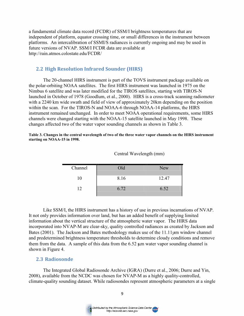
Table 3. Changes in the central wavelength of two of the three water vapor channels on the HIRS instrument

starting on NOAA-15 in 1998.

Central Wavelength (mm)

Channel Old New

10 8.16 12.47

12 6.72 6.52

Like SSM/I, the HIRS instrument has a history of use in previous incarnations of NVAP.

It not only provides information over land, but has an added benefit of supplying limited

information about the vertical structure of the atmospheric water vapor. The HIRS data

incorporated into NVAP-M are clear-sky, quality controlled radiances as created by Jackson and

Bates (2001). The Jackson and Bates methodology makes use of the 11.11 m window channel

and predetermined brightness temperature thresholds to determine cloudy conditions and remove

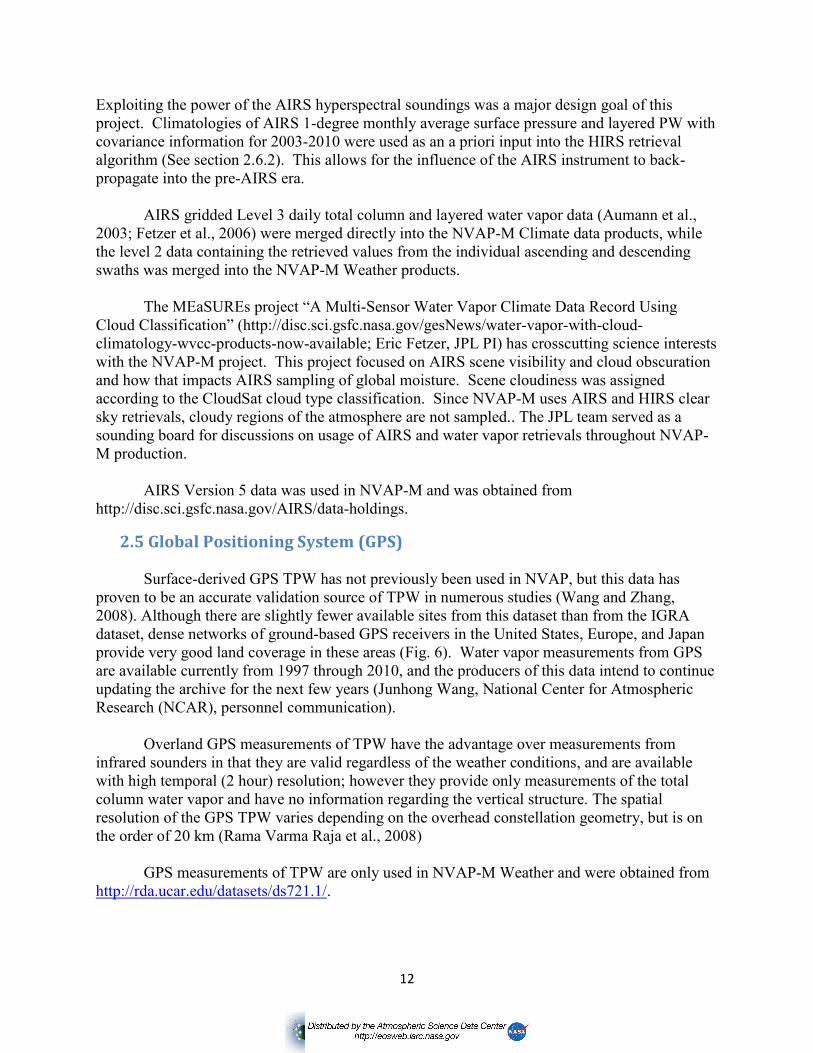
them from the data. A sample of this data from the 6.52 m water vapor sounding channel is

shown in Figure 4.

2.3 Radiosonde

The Integrated Global Radiosonde Archive (IGRA) (Durre et al., 2006; Durre and Yin,

2008), available from the NCDC was chosen for NVAP-M as a highly quality-controlled,

climate-quality sounding dataset. While radiosondes represent atmospheric parameters at a single

10

point, they are a valuable asset to NVAP-M, providing additional observations over land where

HIRS data may not be available or flagged as cloudy. They also provide information about the

vertical structure of the atmosphere, and are available globally (Figure 5) for the duration of the

NVAP-M dataset.

Although the radiosondes have undergone extensive quality control prior to inclusion in

the dataset, some further steps were taken to ensure that only high quality soundings were

considered without unnecessarily excluding a significant number of observations. These

measures were taken specifically to deal with missing layers in the sounding, particularly in the

earliest part of the record. This quality control step requires that 80% of the available sounding

levels below 100 hPa be valid. In general, many missing levels occur at the higher altitudes,

where there is not only very little water vapor in the atmosphere, but also little signal to measure.

The selected threshold of 80% ensures that a majority of the data in the low to mid-troposphere

is available for use, without omitting an excessive number of the available observations. This is

especially important in the early part of the record where less advanced sounding units were used

and missing variables at several levels was a more common occurrence.

Figure 4. Radiances from the 6.52 m water vapor sounding channel of the HIRS/3 instrument on board the

NOAA 16 Satellite for test day September 6, 2002. Grey areas represent missing data due to clouds and orbit

gaps.

11

Figure 5. Distribution of IGRA radiosonde data points for both the standard meteorological and derived

parameter data sets.

2.4 Atmospheric Infrared Sounder (AIRS)

The AIRS instrument is a cross-track scanning infrared spectrometer/radiometer with

2378 channels covering the 3.7 – 15.4 mm spectral range and 4 visible and near-infrared

channels in the 0.4 – 0.94 mm range. AIRS ushered in a new era of hyperspectral sounding of

the atmosphere (Chahine et al., 2006). AIRS was launched on the NASA Aqua spacecraft on

May 4, 2002 into a 705 km sun-synchronous orbit with an expected life-span of 7 years. From

AIRS measurements it is possible to retrieve profiles of atmospheric temperature, relative

humidity and water vapor from the surface to 40 km, as well as surface temperature and

emissivity, surface pressure, rain rate, cloud fraction, and many more variables. Additional

details about the AIRS instrument can be found in Aumann et al. (2003).

AIRS measurements, like all infrared measurements, are susceptible to fields of view that

are obscured by cloud cover, and in the interest of obtaining the maximum amount of

information possible, “cloud cleared” radiances are calculated in these regions. This cloud

clearing methodology attempts to infer clear column radiances in partially cloudy footprints by

using observations from several adjacent fields of view and is described in further detail in

Susskind et al. (2003).

AIRS data products are available in three levels of processing using standard NASA

parlance. Level 1 consists of geolocated radiance and brightness temperatures. Level 2 products

provide instantaneous retrievals of atmospheric parameters with a footprint size of approximately

13.5 km at nadir. Level 3 products provide gridded daily, pentad, 8-day, and monthly values of

level 2 parameters.

AIRS data are used in a variety of ways in NVAP-M, being incorporated as both a source

of ancillary information in retrievals and as a source of water vapor data in the final products.

12

Exploiting the power of the AIRS hyperspectral soundings was a major design goal of this

project. Climatologies of AIRS 1-degree monthly average surface pressure and layered PW with

covariance information for 2003-2010 were used as an a priori input into the HIRS retrieval

algorithm (See section 2.6.2). This allows for the influence of the AIRS instrument to back-

propagate into the pre-AIRS era.

AIRS gridded Level 3 daily total column and layered water vapor data (Aumann et al.,

2003; Fetzer et al., 2006) were merged directly into the NVAP-M Climate data products, while

the level 2 data containing the retrieved values from the individual ascending and descending

swaths was merged into the NVAP-M Weather products.

The MEaSUREs project “A Multi-Sensor Water Vapor Climate Data Record Using

Cloud Classification” (http://disc.sci.gsfc.nasa.gov/gesNews/water-vapor-with-cloud-

climatology-wvcc-products-now-available; Eric Fetzer, JPL PI) has crosscutting science interests

with the NVAP-M project. This project focused on AIRS scene visibility and cloud obscuration

and how that impacts AIRS sampling of global moisture. Scene cloudiness was assigned

according to the CloudSat cloud type classification. Since NVAP-M uses AIRS and HIRS clear

sky retrievals, cloudy regions of the atmosphere are not sampled.. The JPL team served as a

sounding board for discussions on usage of AIRS and water vapor retrievals throughout NVAP-

M production.

AIRS Version 5 data was used in NVAP-M and was obtained from

http://disc.sci.gsfc.nasa.gov/AIRS/data-holdings.

2.5 Global Positioning System (GPS)

Surface-derived GPS TPW has not previously been used in NVAP, but this data has

proven to be an accurate validation source of TPW in numerous studies (Wang and Zhang,

2008). Although there are slightly fewer available sites from this dataset than from the IGRA

dataset, dense networks of ground-based GPS receivers in the United States, Europe, and Japan

provide very good land coverage in these areas (Fig. 6). Water vapor measurements from GPS

are available currently from 1997 through 2010, and the producers of this data intend to continue

updating the archive for the next few years (Junhong Wang, National Center for Atmospheric

Research (NCAR), personnel communication).

Overland GPS measurements of TPW have the advantage over measurements from

infrared sounders in that they are valid regardless of the weather conditions, and are available

with high temporal (2 hour) resolution; however they provide only measurements of the total

column water vapor and have no information regarding the vertical structure. The spatial

resolution of the GPS TPW varies depending on the overhead constellation geometry, but is on

the order of 20 km (Rama Varma Raja et al., 2008)

GPS measurements of TPW are only used in NVAP-M Weather and were obtained from

http://rda.ucar.edu/datasets/ds721.1/.

13

Figure 6. Distribution of GPS data points for which TPW is available from 1997 through 2007. Note that

some stations may come on and off-line and therefore may not be available for the duration of NVAP-M.

2.6 Ancillary Data

2.6.1 Modern Era Retrospective Analysis for Research Applications (MERRA)

The Modern Era Retrospective Analysis for Research and Applications (MERRA) is a

NASA sponsored reanalysis effort designed to use observations from NASA’s EOS satellites

(Aqua, Terra, etc) in a climate context, as well as to improve upon the representation of the

hydrologic cycle from previous reanalyses (Reinecker et al., 2011). The dataset spans most of the

satellite era (1979-present) and was created using the Goddard Earth Observing System (GEOS)

atmospheric model and data assimilation system, incorporating a variety of peer-reviewed

dynamical, physical, and radiative models. It was produced in three processing streams with a

three-year spin-up: two-years at low-resolution followed by 1 year at the final MERRA

resolution.

MERRA represents the only numerical model influence in the NVAP-M product, and it is

a minimal influence at best. An a priori temperature profile is required for use in the infrared

retrieval algorithm. This is obtained from the MERRA “inst3_3d_asm_Cp” product, a 3-hourly

product at 1.25° x 1.25° gridded resolution providing the temperature profile at 42 atmospheric

levels. MERRA products were obtained from http://disc.sci.gsfc.nasa.gov/daac-

bin/FTPSubset.pl.

The HIRS retrieval algorithm determines the appropriate MERRA file based on date, and

extracts the appropriate temperature profile based on the latitude, longitude, and time of the

HIRS footprint. It also determines the lowest valid level of the MERRA profile, failing to

perform the retrieval if the lowest available layer is at or above 100 hPa, or if the lowest

available layer is inconsistent with the a priori surface pressure as determined by AIRS (see

14

section 2.6.2). If the temperature profile is deemed useable, it is averaged into 100 hPa layers for

surface-900 hPa, 900-800 hPa, etc. up to 100 hPa. These 10 layer-mean temperatures act as the a

priori temperature profile in the HIRS retrieval algorithm.

2.6.2 AIRS Climatology

The AIRS instrument is used in NVAP-M not only as a source of total and layered PW,

but also is used in the infrared retrieval algorithm to provide a priori information about the

climatological mean surface pressure and vertical distribution of water vapor in the atmosphere.

AIRS Level 3 1° gridded data for 2003-2010 were used to create monthly climatologies of these

parameters. The Level 3 files include information about a large number of atmospheric and

surface variables, including cloud fraction, which is used in the layered water vapor climatology

calculation.

The AIRS Level 3 water vapor data is available in 12 layers and is given for both

ascending and descending nodes of the satellite orbit. The climatology calculation considers all

available AIRS data files for a given month over the 8 year period. Because the HIRS radiance

data is clear-sky only and no cloud-clearing is attempted, the layered water vapor climatology

was created for those AIRS grid boxes with cloud fraction less than 10% so as not to introduce a

bias in the retrieval.

The ascending and descending swaths for a given day are considered simultaneously. If a

given grid box show less than 10% cloud fraction in both swaths, the water vapor in both swaths

is averaged to represent a daily average value in each layer for that grid box. If the grid box is

less than 10% cloudy in only one swath, then that swath is used to represent the daily average

water vapor for the grid box that day. If both swaths are cloudy, they are not included in the

climatology for that grid box and month. The monthly average layered water vapor is calculated

from these daily average values.

Once the monthly average layered water vapor has been calculated on the 1-degree grid

for all 12 AIRS layers, the layers are then summed to represent the four layers used in NVAP-M

(surface-700 hPa, 700-500 hPa, 500-300 hPa, and 300-100 hPa).

Calculation of the monthly mean surface pressure is performed in a similar manner. The

values obtained in both the ascending and descending nodes are averaged together if they are

both available, or, if only one is available, it is considered to represent the entire day. The daily

average SLP is then used to calculate the monthly average value over the 9-year AIRS period

(2002-2010). Unlike the layered water vapor climatology, the surface pressure climatology has

no dependence on cloud fraction. The mean surface temperature is used in the IR retrieval

algorithm to determine for what layers it should retrieve water vapor (e.g., the surface-700 hPa

layer should not be considered over the Tibetan Plateau). It is also used to determine what layers

of the MERRA temperature profile to include.

15

2.6.3 Sea Surface Temperature

In order to calculate the surface emissivity over the ocean in the passive microwave

retrieval algorithm, a priori information is needed about the sea surface temperature (SST). 1-

degree gridded pentad SST data based on the Reynolds et al. (2002 and 2007) algorithm were

used for this purpose. The data are computed at the NCEP and are available at

http://www.emc.ncep.noaa.gov/research/cmb/sst_analysis/.

The SST product also includes a sea ice mask, which was also employed in the passive

microwave retrieval algorithm to reduce the inclusion of erroneous TPW values in the merged

dataset.

3. Retrieval Algorithms

3.1 Microwave Retrieval Algorithm

In Elsaesser and Kummerow (2008), the authors describe a retrieval algorithm designed

for use over non-raining oceanic scenes to obtain the sea surface wind speed, total precipitable

water, and cloud liquid water (CLW) from passive microwave radiance observations. The

authors also noted a characteristic behavior of the retrieval’s diagnostic outputs when

precipitation was present in the scene. We have chosen to use this algorithm to retrieve TPW

from the SSM/I radiances, and to use these diagnostic outputs to screen for precipitating scenes

rather than to rely on a statistical algorithm such as Grody (1991) or Ferraro (1998) as was done

in the heritage version of NVAP. The Elsaesser and Kummerow algorithm was selected over the

Greenwald et al. (1993) algorithm that was used in the heritage NVAP dataset. This algorithm

provides many advantages, including the more physically-based precipitation screen, sensor

independence, and the use of peer-reviewed radiative transfer models. The algorithm is

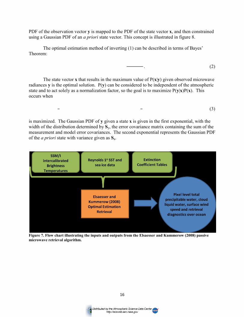
discussed below, and a chart illustrating data flow through the algorithm is shown in Figure 7.

The selected retrieval is an optimal estimation algorithm described by Rodgers (1976,

1990, and 2000) and based on the premise that the relationship between the measured properties

of atmospheric radiation and the atmospheric state can be expressed by

y = f(x,b) + , (1)

where y represents the radiance measurements at each channel, f(x,b) is a forward model

representing atmospheric and radiative processes with x representing the atmospheric parameters

of interest (the “state vector”) and b representing atmospheric parameters that are considered

known or reasonably assumed in the forward model (such as SST). represents a general error

term, accounting for errors in measurements, assumptions and model physics. Given

measurements y and assumptions b, the goal is to invert (1) to solve for x.

The general premise of an optimal estimation retrieval is to describe the value of a given

parameter as a probability distribution function (PDF) with some mean and variance 2. The

16

PDF of the observation vector y is mapped to the PDF of the state vector x, and then constrained

using a Gaussian PDF of an a priori state vector. This concept is illustrated in figure 8.

The optimal estimation method of inverting (1) can be described in terms of Bayes’

Theorem:

. (2)

The state vector x that results in the maximum value of P(x|y) given observed microwave

radiances y is the optimal solution. P(y) can be considered to be independent of the atmospheric

state and to act solely as a normalization factor, so the goal is to maximize P(y|x)P(x). This

occurs when

(3)

is maximized. The Gaussian PDF of y given a state x is given in the first exponential, with the

width of the distribution determined by Sy, the error covariance matrix containing the sum of the

measurement and model error covariances. The second exponential represents the Gaussian PDF

of the a priori state with variance given as Sa.

Figure 7. Flow chart illustrating the inputs and outputs from the Elsaesser and Kummerow (2008) passive

microwave retrieval algorithm.

17

Figure 8. Illustration of the optimal estimation retrieval algorithm process, where the black oval represents

the set of possible atmospheric states, the blue oval the set of states that could be represented by the

observations, and the purple oval the a priori constraint. The optimal solution is found in the intersection of

these three ovals, shown in orange.

The maximum of (3) is found when the cost function is minimized, i.e., where the

probability that x accurately represents the atmospheric state is the greatest. is given by

The forward model is then further linearized about a base state xi (Rodgers, 2000).

Newtonian iteration is then employed to reach the solution by

, (5)

where K is a weighting function matrix that indicates the sensitivity of the linearized forward

model to a change in the state parameter, and xi+1 is the optimal solution that is reached when the

difference between xi+1 and xi is an order of magnitude smaller than the estimated error variance

of the state in the current iteration. The estimated error variance is determined by the number of

retrieved parameters and is discussed in detail in Rodgers (2000).

The forward radiative model (f(x,b)) assumes a non-scattering (i.e., non-precipitating),

plane-parallel atmosphere. Over the oceanic surfaces of interest, the emission and reflection of

microwave radiation is calculated using a specular emissivity model based on Deblonde and

English (2001), which uses the wind speed, SST, and radiometer frequency. A rough sea surface

model based on Kohn (1995) and Wilheit (1979a, b) is also used. Atmospheric absorption by

nitrogen, oxygen and water vapor is calculated with a version of the Rozenkranz (1998) model

with a slight modification to absorption line width and intensity, especially at the 22-GHz water

vapor line. Assuming that cloud liquid water droplets are small enough to use the Rayleigh

approximation, absorption by cloud liquid water is calculated using the model of Liebe et al.

(1991) and Liebe et al. (1993).

A priori estimates of surface wind, TPW and CLW were acquired as the global annual

mean derived from the Advanced Microwave Scanning Radiometer for EOS (AMSR-E) by

18

Remote Sensing Systems (RSS). Ancillary data includes SST obtained from Reynolds et al.

(2002 and 2007) and zonal average temperature lapse rate and water vapor profiles for 1998

derived from European Center for Medium Range Weather Forecasts Reanalysis-40 (ECMWF

ERA-40) at T159 spectral resolution (~1.125°). Although these zonal averages and a priori

values are not globally representative, lack a seasonal cycle, and demonstrate a high degree of

uncertainty, Elsaesser and Kummerow (2008) note a low sensitivity of the retrieval to them.

Output from the optimal estimation retrieval includes several diagnostic variables that

indicate the retrieved parameters’ level of dependence on the observations and a priori and how

well the forward model assumptions and assumed error covariances agree with the observed

scene (Chi-Square value, 2). If 2 is large, the forward model does not accurately represent the

physical state of the observed scene. Since the forward model is designed to work in non-

precipitating scenes, it follows that such scenes would have a large 2 value. This behavior was

noted in Elsaesser and Kummerow (2008), where 2 > 40 was used to accurately screen for

precipitation in oceanic cases. In order to be conservative with respect to including footprints

contaminated by precipitation, this threshold was lowered to 35 for use in NVAP-M.

Results from the optimal estimation retrieval were compared with several independent

datasets, including radiosonde, GPS, and Version 6 retrieved TPW from RSS (Wentz, 1997).

Radiosonde and GPS data points were matched to SSM/I footprints that occurred within 0.5° and

30 minutes of the ground measurement and generally represent coastal or island stations. The

larger available number of GPS comparisons is due to the fact that GPS observations are made

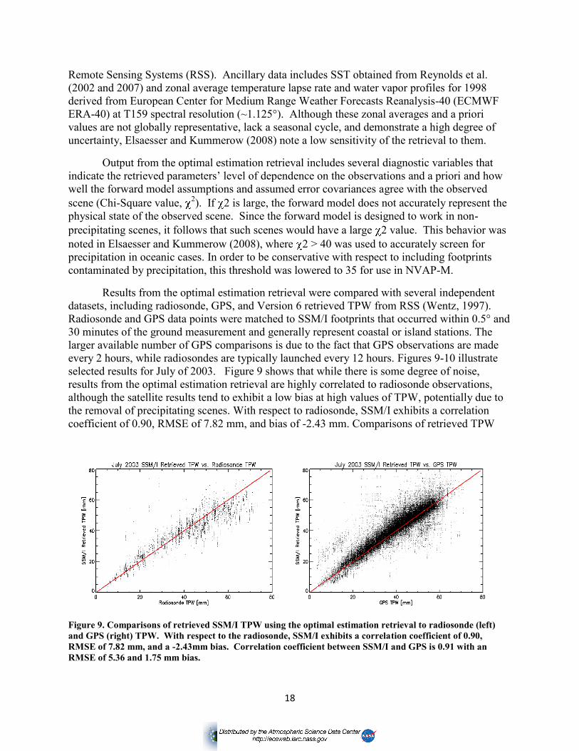
every 2 hours, while radiosondes are typically launched every 12 hours. Figures 9-10 illustrate

selected results for July of 2003. Figure 9 shows that while there is some degree of noise,

results from the optimal estimation retrieval are highly correlated to radiosonde observations,

although the satellite results tend to exhibit a low bias at high values of TPW, potentially due to

the removal of precipitating scenes. With respect to radiosonde, SSM/I exhibits a correlation

coefficient of 0.90, RMSE of 7.82 mm, and bias of -2.43 mm. Comparisons of retrieved TPW

Figure 9. Comparisons of retrieved SSM/I TPW using the optimal estimation retrieval to radiosonde (left)

and GPS (right) TPW. With respect to the radiosonde, SSM/I exhibits a correlation coefficient of 0.90,

RMSE of 7.82 mm, and a -2.43mm bias. Correlation coefficient between SSM/I and GPS is 0.91 with an

RMSE of 5.36 and 1.75 mm bias.

19

with surface-based GPS stations continue to show a high amount of scatter, with a correlation

coefficient of 0.9, RMSE of 5.36 mm and a slight high bias of 1.75 mm over all values of TPW.

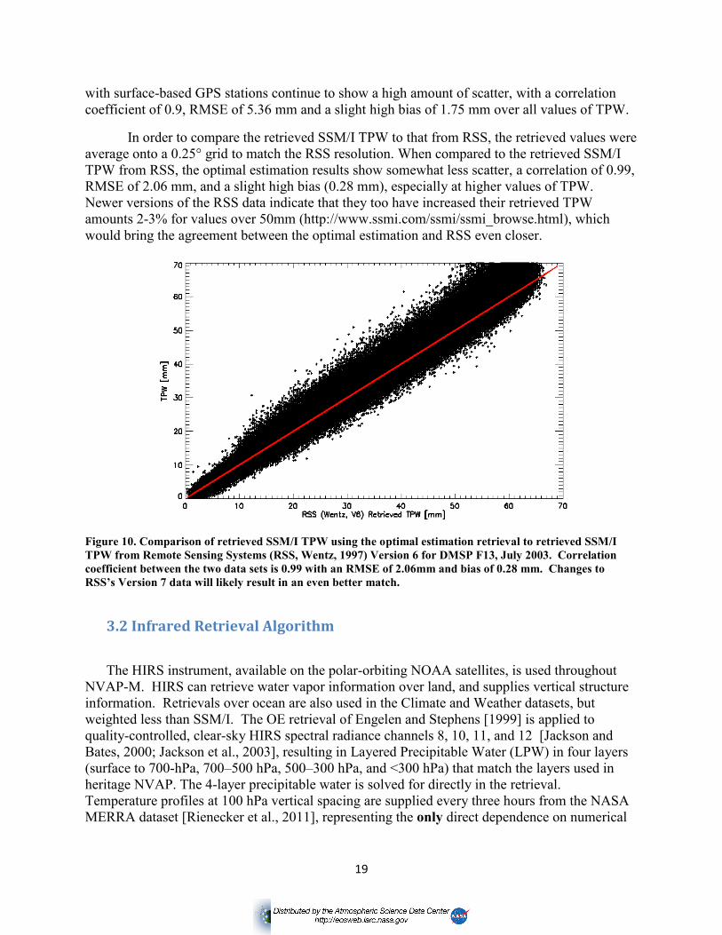
In order to compare the retrieved SSM/I TPW to that from RSS, the retrieved values were

average onto a 0.25° grid to match the RSS resolution. When compared to the retrieved SSM/I

TPW from RSS, the optimal estimation results show somewhat less scatter, a correlation of 0.99,

RMSE of 2.06 mm, and a slight high bias (0.28 mm), especially at higher values of TPW.

Newer versions of the RSS data indicate that they too have increased their retrieved TPW

amounts 2-3% for values over 50mm (http://www.ssmi.com/ssmi/ssmi_browse.html), which

would bring the agreement between the optimal estimation and RSS even closer.

Figure 10. Comparison of retrieved SSM/I TPW using the optimal estimation retrieval to retrieved SSM/I

TPW from Remote Sensing Systems (RSS, Wentz, 1997) Version 6 for DMSP F13, July 2003. Correlation

coefficient between the two data sets is 0.99 with an RMSE of 2.06mm and bias of 0.28 mm. Changes to

RSS’s Version 7 data will likely result in an even better match.

3.2 Infrared Retrieval Algorithm

The HIRS instrument, available on the polar-orbiting NOAA satellites, is used throughout

NVAP-M. HIRS can retrieve water vapor information over land, and supplies vertical structure

information. Retrievals over ocean are also used in the Climate and Weather datasets, but

weighted less than SSM/I. The OE retrieval of Engelen and Stephens [1999] is applied to

quality-controlled, clear-sky HIRS spectral radiance channels 8, 10, 11, and 12 [Jackson and

Bates, 2000; Jackson et al., 2003], resulting in Layered Precipitable Water (LPW) in four layers

(surface to 700-hPa, 700–500 hPa, 500–300 hPa, and <300 hPa) that match the layers used in

heritage NVAP. The 4-layer precipitable water is solved for directly in the retrieval.

Temperature profiles at 100 hPa vertical spacing are supplied every three hours from the NASA

MERRA dataset [Rienecker et al., 2011], representing the only direct dependence on numerical

20

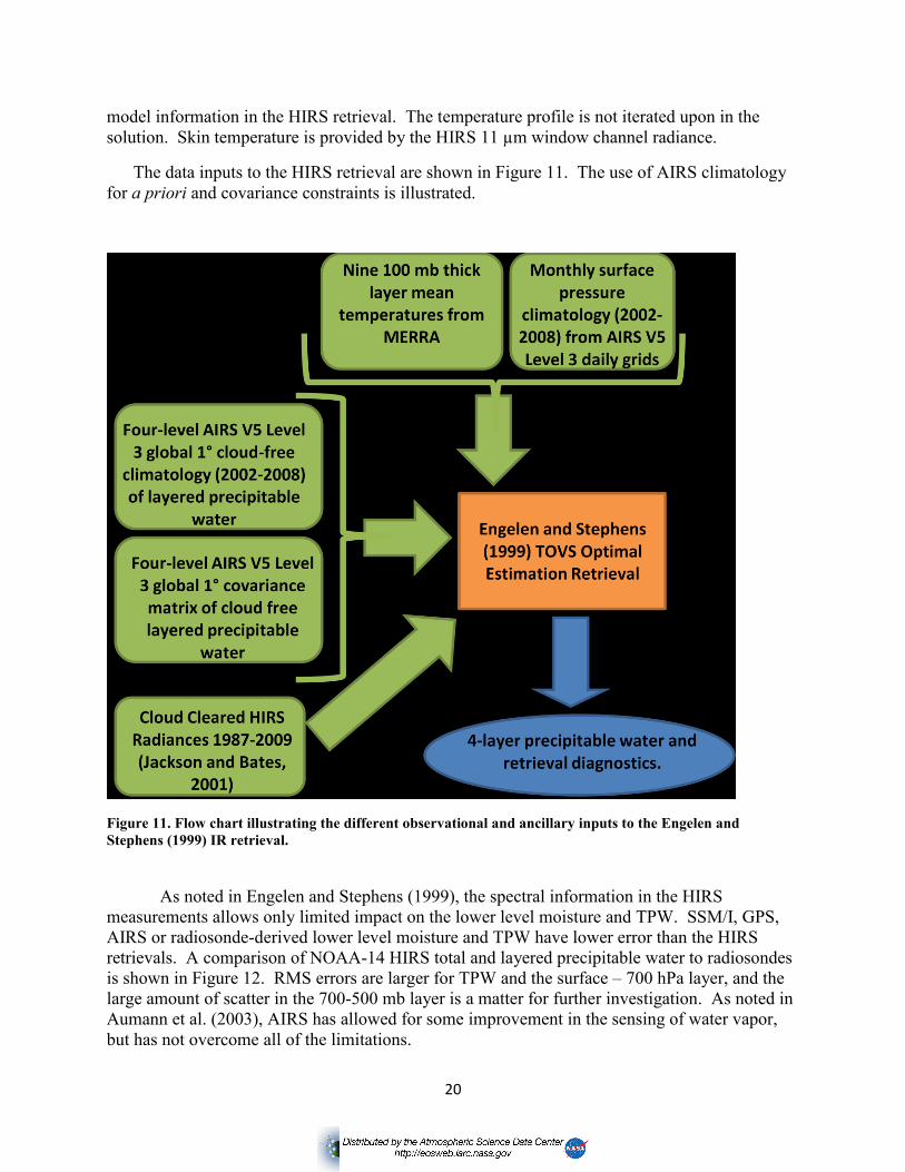
model information in the HIRS retrieval. The temperature profile is not iterated upon in the

solution. Skin temperature is provided by the HIRS 11 µm window channel radiance.

The data inputs to the HIRS retrieval are shown in Figure 11. The use of AIRS climatology

for a priori and covariance constraints is illustrated.

Figure 11. Flow chart illustrating the different observational and ancillary inputs to the Engelen and

Stephens (1999) IR retrieval.

As noted in Engelen and Stephens (1999), the spectral information in the HIRS

measurements allows only limited impact on the lower level moisture and TPW. SSM/I, GPS,

AIRS or radiosonde-derived lower level moisture and TPW have lower error than the HIRS

retrievals. A comparison of NOAA-14 HIRS total and layered precipitable water to radiosondes

is shown in Figure 12. RMS errors are larger for TPW and the surface – 700 hPa layer, and the

large amount of scatter in the 700-500 mb layer is a matter for further investigation. As noted in

Aumann et al. (2003), AIRS has allowed for some improvement in the sensing of water vapor,

but has not overcome all of the limitations.

21

Figure 12: Comparison of HIRS retrieved TPW and LPW for three layers versus adjacent radiosondes

within 2 hours and 100 km. RMS errors are shown, along with the 1:1 line in red.

4. Merging of Water Vapor Data into a Single Product

The merge procedure is the same for all production streams (Climate, Weather, and

Ocean). Only the appropriate input datasets and spatial and temporal resolution are altered.

First, the microwave and infrared retrievals are performed on each field of view. All of the fields

of view from each satellite over the appropriate time period (daily for the Climate and Ocean

products, 6-hourly for the Weather product) are then averaged onto a 1° (Climate, Ocean) or 0.5°

(Weather) grid. This results in gridded TPW and LPW maps for each available SSM/I, HIRS,

and AIRS. A single radiosonde or GPS data point is assumed to represent the grid box it

occupies; or, if multiple data points are available within a given grid box, they are averaged.

Next, gridded TPW and LPW from like sensors are averaged together, resulting in a

single TPW and LPW map for each platform (SSM/I, HIRS, etc.). Next, an error-weighted

averaging technique combines all available TPW/LPW observations for a given day (or 6-hour

period for NVAP-M Weather). A variance has been determined for each sensor based on

comparisons with either other observations or with published values. The variance values for

each sensor are shown in table 4.

The variance is used to determine how much weight a given sensor is given in the merge

process by:

22

where wi is the weight assigned to the observation from instrument i and σ2 is the variance

assigned to that sensor. TPW in a given grid box is then calculated as

Table 4. Assigned variance values for the instruments merged into NVAP-M.

Instrument SSM/I HIRS Radiosonde GPS AIRS

Variance (mm) 3.0 10.0 2.0 1.0 3.0

where vi represents the average water vapor in a given grid box from instrument i and n is the

total number of instruments being merged. This process is performed for both total and layered

water vapor. However, due to the combination of observations from multiple sensors, is it

possible that the sum of the layered PW in a grid box will not equal the TPW value listed in the

same grid box and time. For example, a grid box containing valid observations from SSM/I and

HIRS only would combine TPW estimates from both sensors, but the LPW estimate would

contain values from HIRS only.

5. References

Aumann, H. H., M. T. Chahine, C. Gautier, M. D. Goldberg, E. Kalnay, L. M. McMillin, H.

Revercomb, P. W. Rosenkranz, W. L. Smith, D. H. Stelin, L. L. Strow, and J. Susskind,

2003: AIRS/AMSU/HSB on the Aqua mission: Design, science objectives, data products,

and processing systems. IEEE Trans. Geosci. Remote Sens., 41, 2, 253 – 264.

Chahine, M. T. and coauthors, 2006: AIRS: Improving weather forecasting and providing new

data on greenhouse gases. Bull. Amer. Meteorol. Soc., 87, 911-926.

Deblonde, G., and S. J. English, 2001: Evaluation of the FASTEM-2 fast microwave ocean

surface emissivity model. Tech. Proc. Int. TOVS Study Conf. XI, Budapest, Hungary,

WMO, 67 – 78.

Durre, I, R. S. Vose, and D. V. Wuertz, 2006: Overview of the Integrated Global Radiosonde

Archive. J. Climate, 19, 53-68.

Durre, I., and X. Yin, 2008: Enhanced radiosonde data for studies of vertical structure. Bull.

Amer. Meteor. Soc., 89, 1257-1262.

Elsaesser, G. S. and C. D. Kummerow, 2008: Towards a fully parametric retrieval of the non-

raining parameters over the global ocean. J. Appl. Meteor. & Climatol., 47, 1590 – 1598.

23

Engelen, R. J. and G. L. Stephens, 1999: Characterization of water-vapour retrievals from

TOVS/HIRS and SSM/T2 measurements. Q.J.R. Meteorol. Soc., 125, 331 – 351.

Eskridge, R. E., O. A. Alduchov, I. V. Chernykh, Z. Panmao, A. C. Polansky and S. R.Doty,

1995: A Comprehensive Aerological Reference Data Set (CARDS): Rough and

systematic errors. Bull. Amer. Meteor. Soc., 76, 1759–1775.

Ferraro, R. R., E. A. Smoth, W. Berg, and G. J. Huffman, 1998: A screening methodology for

passive microwave precipitation retrieval algorithms. J. Atmos. Sci., 55, 1583 – 1600.

Fetzer, E. J., B. H. Lambrigtsen, A. Eldering, H. H. Aumann, and M. T.Chahine (2006), Biases

in total precipitable water vapor climatologies from Atmospheric Infrared Sounder and

Advanced Microwave Scanning Radiometer, J. Geophys. Res., 111, D09S16,

doi:10.1029/2005JD006598

Fetzer, E. J. and coauthors, 2012: A multi-sensor water vapor climate data record using cloud

classification. Dataset. Available at http://disc.sci.gsfc.nasa.gov/daac-

bin/DataHoldingsMEASURES.pl?PROGRAM_List=EricFetzer

Goodlum, G., K. B. Kidwell, and W. Winston, Eds., 2000: NOAA KLM Users Guide.

http://www2.ncdc.noaa.gov/docs/klm/index.htm

Greenwald, T. J., G. L. Stephens, T. H. Vonder Haar, and D. L. Jackson, 1993: A physical

retrieval of cloud liquid water over global oceans using Special Sensor Microwave /

Imager (SSM/I) observations. J. Geophys. Res., 98, 18471-18488.

Grody, N. C., 1991: Classification of snow cover and precipitation using the special sensor

microwave imager. J. Geophys. Res., 96, D4, 7423 – 7435.

Hollinger, J. P., J. L. Peirce, and G. E. Poe, 1990: SSM/I Instrument Evaluation. IEEE Trans.

Geosci. Remote Sens., 28, 781 – 790.

Jackson, D.L., and J.J. Bates, 2000: A 20-yr TOVS Pathfinder data set for climate analysis.

Tenth Conference on Satellite Meteorology and Oceanography/, Long Beach, CA,

January 10-14, 2000.

Jackson, D.L., J.J. Bates, and D. Wylie, 2003: The HIRS Pathfinder Radiance data set (1979-

2001). 12th Conference on Satellite Meteorology and Oceanography, Long Beach,

California, February 10-13, 2003.

Kanamitsu, M., W. Ebisuzaki, J. Woollen, S-K. Yang, J.J. Hnilo, M.Fiorinot, and G. L. Potter,

2002: NCEP-DOE AMIP II Reanalysis (R-2). Bull. Amer. Meteorol. Soc., 83, 1631-

1643.

Kidwell, K. B., Ed. 1998: NOAA Polar Orbiter Data User’s Guide. U.S Department of

24

Commerce, National Oceanic and Atmospheric Administration, National Environmental

Satellite, Data and Information Service, National Climatic Data Center. Available online:

http://www.ncdc.noaa.gov/oa/pod-guide/ncdc/docs/podug/cover.htm

Kohn, D. J., 1995: Refinement of a semi-empirical model for the microwave emissivity of the

sea surface as a function of wind speed. M.S. thesis, Dept of Meteorology, Texas A&M

University, 44 pp.

Leibe, H. G., G. A. Hufford, and T. Manabe, 1001: A model for the complex permittivity of

water at frequencies below 1THz. Int. J. Infrared Millimeter Waves, 12, 659 – 675.

_____, _____, and M. G. Cotton, 1993: Propagation modeling of moist air and suspended water

particles at frequencies below 1000 GHz. Advisory Group for Aerospace Research and

Development Conf. Proc: Atmospheric Propagation Effects through Natural and Man-

Made Obscurants for Visible to mm-wave Radiation (AGARD-CP-542), AGARD,

Neuilly sur Seine, France, 3-1 – 3-10.

Maloney, E. D. and S. K. Esbensen, 2003: The Amplification of East Pacific Madden–Julian

Oscillation Convection and Wind Anomalies during June–November J. Climate, 16,

3482–3497.

Rama Varma Raja, M. K., S. I. Gutman, J. G. Yoe, L.M. McMillin, and J. Zhao, 2008: The

validation of AIRS retrievals of integrated precipitable water vapor using measurements

from a network of ground-based GPS receivers over the contiguous United States. J.

Atmos. Oceanic. Tech., 25, 416-428.

Randel, D. L., T. H. Vonder haar, M. A. Ringerud, G. L. Stephens, T. J. Greenwald and C. L.

Combs, 1996: A new global water vsapor dataset. Bull. Amer. Meteor. Soc., 77, 1233 –

1246.

Rienecker, M. M., et al. (2011), MERRA-NASA’s Modern-Era Retrospective

Analysis for Research and Applications, J. Clim., 24, 3624–3648,

doi:10.1175/JCLI-D-11-00015.1.

Reynolds, R. W., N. A. Rayner, T. M. Smith, D. C. Stokes, and W. Wang, 2002: An improved in

situ and satellite SST analysis for climate. J. Climate, 15, 1609 – 1625.

Reynolds, Richard W., Thomas M. Smith, Chunying Liu, Dudley B. Chelton, Kenneth S. Casey,

Michael G. Schlax, 2007: Daily High-Resolution-Blended Analyses for Sea Surface

Temperature. J. Climate, 20, 5473–5496. doi: http://dx.doi.org/10.1175/2007JCLI1824.1

Robel, J., Ed., 2009: NOAA KLM User’s Guide. U.S. Department of Commerce, National

Oceanic and Atmospheric Administration, National Environmental Satellite, Data, and

Information Service. Available online:

http://www.ncdc.noaa.gov/oa/pod-guide/ncdc/docs/klm/cover.htm

25

Rodgers, C. D., 1976: Retrieval of atmospheric temperature and composition from remote

measurements of thermal radiation. Rev. Geophys. Space Phys., 14, 609 – 624.

_____, 1990: Characterization and error analysis of profiles retrieved from remote ounding

measurements. J. Geophys. Res., 95, 5587 – 5595.

_____, 2000: Inverse Methods for Atmospheric Sounding: Theory and Practice. World Scientific

Publishing Co., Singapore, 238pp.

Rozenkranz, P. W., 1998: Water vapor microwave continuum absorption: A comparison of

measurements and models. Radio Sci., 33, 919 – 928.

Sapiano, M. R. P., W. K. Berg, D. S. McKague, and C. D. Kummerow, 2012: Toward an

intercalibrated fundamental climate data record of the SSM/I sensors. IEEE Trans.

Geosci. Remote Sens., in press.

Simpson, J. J., J. S. Berg, C. J. Koblinsky, G. L. Hufford, and B. Beckley, 2001: The NVAP

global water vapor dataset: independent cross-comparison and multiyear variability.

Remote Sens. Environ., 76, 112-129.

Susskind, J., C. D. Barnett, and J. M. Blaisdell, 2003: Retrieval of atmospheric and surface

parameters from AIRS/AMSU/HSB data in the presence of clouds. IEEE Trans. Geosci.

Remote Sens., 41, 2, 390 – 409.

Trenberth, K. E., J. Fasullo, and L. Smith, 2005: Trends and variability in column-integrated

atmospheric water vapor. Climate Dynamics, 24, 741-758.

Vonder Haar, T. H., J.M. Forsythe, D. McKague, D. L. Randel, B. C. Ruston, and S. Woo, 2003:

Continuation of the NVAP Global Water Vapor Data Sets for Pathfinder Science

Analysis. Science and Technology Corp., STC Technical Report 3333, 44 pp.

http://eosweb.larc.nassa.gov/PRODOCS/nvap/sci_tech_report_3333.pdf.

Vonder Haar, T. H., J. L. Bytheway and J. M. Forsythe, 2012: Weather and climate analyses

using improved global water vapor observations. Geophys. Res. Lett., 39, L16802,

doi:10.1029/2012GL052094.

Wang, J., L. Zhang, A. Dai, T. Van Hove, and J. Van Baelen, 2007: A near-global, 2-hourly data

set of atmospheric precipitable water from ground-based GPS measurements. J. Geophys.

Res., 112. doi:10.1029/2006JD007529.

______, and _____, 2008: Systematic errors in global radiosonde precipitable water data from

comparisons with ground-based GPS measurements. J. Climate, 21, 2218-2238.

Wentz, F. J., 1997: A well-calibrated ocean algorithm for special sensor microwave/imager. J.

Geophys. Res., 102 (C4), 8703 - 8718.

26

Wilheit, T. T., 1979a: A model for the microwave emissivity of the ocean’s surface as a function

of wind speed. IEEE Trans. Geosci. Electron., 17, 244–249.

——, 1979b: The effect of wind on the microwave emission from the ocean’s surface at 37 GHz.

J. Geophys. Res., 84, 4921–4926.

Zeng, X. and E. Lu, 2004: Globally Unified Monsoon Onset and Retreat Indexes. J. Climate, 17,

2241–2248.

Appendix A: Dataset Description

A.1 Naming Convention

NVAP-M products are available in NetCDF format. File names are as follows:

YYYY.JJJ.NVAPs.PPP.Txdaily.nc

Where

YYYY = four digit year (1988-2009)

JJJ = three digit Julian day (1-366)

s = one character denoting the processing “tier” (C for Climate, S for Synoptic (Weather), O for

Ocean)

PPP= three character data type (tpw or lyr)

T = one digit number of times daily the data is available (1 or 4)

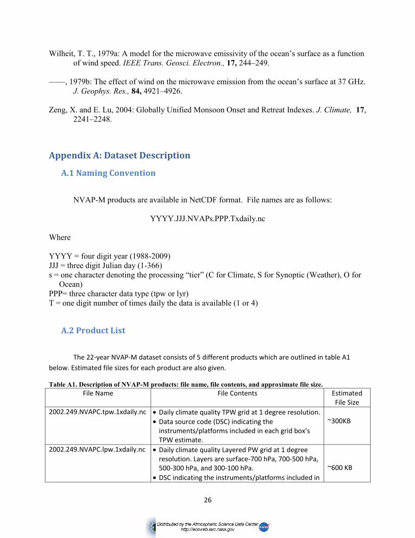
A.2 Product List

The 22-year NVAP-M dataset consists of 5 different products which are outlined in table A1

below. Estimated file sizes for each product are also given.

Table A1. Description of NVAP-M products: file name, file contents, and approximate file size.

File Name File Contents Estimated File Size

2002.249.NVAPC.tpw.1xdaily.nc Daily climate quality TPW grid at 1 degree resolution.

Data source code (DSC) indicating the instruments/platforms included in each grid box’s TPW estimate.

~300KB

2002.249.NVAPC.lpw.1xdaily.nc Daily climate quality Layered PW grid at 1 degree resolution. Layers are surface-700 hPa, 700-500 hPa, 500-300 hPa, and 300-100 hPa.

DSC indicating the instruments/platforms included in

~600 KB

27

the PW estimate for each grid box and layer.

2002.249.NVAPS.tpw.4xdaily.nc 6-hourly NVAP-M Weather TPW grid at 0.5 degree resolution.

DSC indicating which instruments/platforms are included in the TPW estimate in each grid box.

~2.5 MB

2002.249.NVAPS.lpw.4xdaily.nc 6-hourly NVAP-M Weather Layered PW at 0.5 degree resolution. Layers are the same as those for NVAP-M Climate product.

DSC indicating which instruments/platforms are included in the PW estimate for each grid box and layer.

~ 7.0 MB

2002.249.NVAPO.tpw.1xdaily.nc Daily, ocean-only TPW from SSM/I only on a 1 degree grid.

DSC indicating which SSM/I platforms were included in the TPW estimate for each grid box.

~ 150 KB

Appendix B: Acronyms

AIRS: Atmosphere Infrared Sounder

AMSR-E: Advanced Microwave Scanning Radiometer for EOS

AMSU: Advanced Microwave Sounding Unit

ASDC: Atmospheric Science Data Center

ATOVS: Advanced TOVS

CARDS: Comprehensive Aerological Reference Data Set

CLW: Cloud Liquid Water

DMSP: Defense Meteorological Satellite Program

DoD: Department of Defense

DSC: Data Source Code

ECMWF: European Center for Medium-Range Weather Forecasts

EOS: Earth Observing System

ERA-40: ECMWF Reanalysis

ESDR: Earth System Data Record

FCDR: Fundamental Climate Date Record

GEOS: Goddard Earth Observing System

GOES: Geostationary Operational Environmental Satellites

GPS: Global Positioning Satellite

HIRS: High Resolution Infrared Radiation Sounder

IDL: Interactive Data Language

IGRA: Integrated Global Radiosonde Archive

MEaSUREs: Making Earth Science Data Records for Use in Research Environments

MERRA: Modern Era Retrospective-Analysis for Research and Applications

NASA: National Aeronautics and Space Administration

NCAR: National Center for Atmospheric Research

NCDC: National Climatic Data Center

28

NCEP: National Center for Environmental Prediction

NOAA: National Oceanic and Atmospheric Administration

NVAP: NASA Water Vapor Project

NVAP-M: NVAP-MEaSUREs

NVAP-NG: NVAP-Next Generation

PDF: Probability distribution function

PW: precipitable water

RSS: Remote Sensing Systems

SSM/I: Special Sensor Microwave/Imager

SSMI/S Special Sensor Microwave Imager/Sounder

SSM/T-2: Special Sensor Microwave/Temperature Sounder

SST: Sea Surface Temperature

STC-METSAT: Science and Technology Corp., METSAT Division

TIROS: Television Infrared Observation Satellite

TOVS: TIROS Operational Vertical Sounder

TPW: Total Precipitable Water

Appendix C: Discussion of artifacts due to changes in satellite sampling

Despite the use of constant algorithms and intercalibrated input datasets through time,

there are still time-dependent artifacts present in the NVAP-M Climate dataset, including

significant dry anomalies in the tropics during the early period of the dataset (1988-1992) and an

apparent global moistening starting in 1995. These anomalies have been traced to the variations

in satellite sampling with time. Figure 2 in the main text shows the available input sources with

time. The number of platforms carrying SSM/I varies between 1 and 3, while there are up to 4

HIRS instruments available at once.

Figure A1 shows a time series of the monthly average area covered by each instrument,

with the data from infrared instruments broken into total, ocean, and land values. This figure

indicates that, no matter how many instruments are available, the potential area of the globe that

can be observed is asymptotic at about 50%. This is not surprising, since SSM/I can only retrieve

water vapor over the ocean, which represents 70% of the earth, and it cannot retrieve water vapor

in regions of heavy precipitation, over ice, or in the gaps between orbits. HIRS radiances are

clear-sky only, which represents an average of only 30% of the earth, however the presence of

HIRS on multiple satellites passing over a given region at different times allows for more

observations if clouds have moved out of the area.

29

Figure A1. Monthly mean area of total coverage for all instruments used in NVAP-M Climate (solid)

including SSM/I (black), HIRS (red), AIRS (blue) and radiosonde (green). Infrared instruments (HIRS and

AIRS) are broken down into average coverage area for ocean (dotted) and land (dashed) as well. The area covered by AIRS is significantly less than that of the other sensors. This is due

to the way cloudy scenes were removed from the dataset. HIRS retrievals are performed on each

individual field of view (FOV), and then the FOVs are averaged onto a 1 degree grid. If a grid

box contains both clear and cloudy FOVs, the clear FOVs are used to calculate the grid box

average TPW. As such, even grid boxes with 90% cloud could have clear footprints within them

that are assumed to represent the entire box. The AIRS Level 3 data is already in a 1 degree

gridded format, and each grid box has a retrieved cloud fraction. For use in NVAP-M, AIRS grid

boxes with greater than 10% cloud fraction were omitted. In essence, the cloud removal

technique for AIRS is more conservative than that used with HIRS, thus decreasing the overall

global coverage obtained from AIRS.

The time-dependent artifacts seen in figure1 of the main text can be explained in part

using figures A1 and A2. Starting with the unusually try tropics seen in the first 4 years of the

record, we see that the driest periods correspond with slight decreases in coverage by SSM/I, and

in fact the largest dry anomaly extending from the tropics through most of the southern

hemisphere corresponds with a significant drop in SSM/I sampling of the tropical oceans, where

HIRS is unable to compensate due to the persistently cloudy nature of the region. In fact, from

late 1989 through the first half of 1990, there do not appear to be any notable artifacts, during a

period when SSM/I was operating normally.

30

Figure A2. Ratio of the monthly mean area land and ocean area covered by the infrared instruments used in

NVAP-M Climate.

The apparent global moistening that began in 1995 and continued through the late 1990s

can similarly be explained by a decrease in sampling from the HIRS instrument. In 1995, the

HIRS instruments on NOAA-11 and NOAA-12 were experiencing some end-of-life issues. As a

result, while some data is still available from these instruments past that point, it is temporally

spotty and of questionable quality. As a result, the use of data from these two sensors was

discontinued when NOAA-14 became available, quickly reducing the number of available HIRS

instruments from a potential 3 to 1. Because HIRS radiances are a primary source of information

over land and the radiances globally were clear-sky only, it was essentially being used to observe

the driest portions of the dataset. Additionally, as can be seen in Fig. A1, coverage over land was

impacted somewhat more than coverage over ocean. As a result, SSM/I observations dominate

over the ocean, and fewer land observations are available for inclusions in the global average,

leading to an apparent moist anomaly during this period.

The impact of changing sampling through time on trend detection remains to be studied.

Vonder Haar et al. (2012) stated “Therefore, at this time, we can neither prove nor disprove a

robust trend in the global water vapor data”.

Appendix D: Frequently Asked Questions

Below are some of the frequently asked questions regarding the NVAP-M dataset.

1. Where is the NVAP data located?

Heritage NVAP data can be found online at

http://eosweb.larc.nasa.gov/PRODOCS/nvap/table_nvap.html

31

The NVAP-M dataset completely supercedes the heritage dataset, and users

should use NVAP-M.

The new NVAP-M can be found online at the NASA Langley Atmospheric Science

Data Center (ASDC) .

2. What is the data format?

The NVAP dataset is provided in gridded NetCDF files at either one or half-degree

resolution.

3. Which NVAP-M product should I use, weather, climate or ocean?

The weather version of NVAP-M contains higher spatial and temporal resolution than

does the climate version. It combines input from a larger number of sensors than the

climate version, using sensors that are not available over the course of the entire

dataset. That is, it does not use the same consistent inputs through time as the climate

version. There may be areas where data is not available in any six hour grid. You

should use this data if you are planning a case study of a specific meteorological event

or phenomenon, testing a short to mid-range forecast, or if you are only interested in a

very small area.

The climate version of NVAP-M contains a gridded daily average water vapor value at

one degree resolution. The sensors used in creating this dataset have a long stable

record, and there have been no changes in processing methodology over the course of

the dataset. There should be minimal areas of missing data, particularly during periods

with many available satellite platforms. You should use this dataset if you are

interested in global trends or variability over a long period of time.

The ocean only version of NVAP-M contains gridded daily average TPW only over

oceanic scenes using only input data from SSM/I. You should use this product if you

are interested in only oceanic scenes or comparisons with other ocean only, passive

microwave TPW datasets.

4. What is more reliable, TPW or LPW?

TPW is the most reliable geophysical quantity in NVAP-M due to the use of GPS (in

NVAP-M Weather) and passive microwave inputs. The LPW fields improve from 2003

onwards with the use of AIRS. It should be noted though that AIRS and HIRS are subject

to the same biases by rejecting cloudy scenes. See the MEaSUREs project of Fetzer et al.

(2012) for more information on this effect.

5. Why wasn’t more spatial or temporal extrapolation applied?

The goal of NVAP-M was not to create daily or more frequent images with no holes via

smoothing. Heritage NVAP did extrapolate to achieve this; however the limitations of the

32

varied inputs are simply carried forth in NVAP-M. Users interested in greater

extrapolation and smoothing can apply these irreversible processes themselves. The

NVAP-M weather dataset and companion data source code could be used to achieve this

goal.

6. Is there any NVAP-M data beyond 2009?

At the time of this writing (early 2013) no effort to continue the NVAP-M dataset has

been funded.