NASA Contractor Report 198228

ICASE Report No. 95-73

I CASE EFFICIENT IMPLEMENTATION OF WEIGHTED ENO SCHEMES

Guang-Shan Jiang Chi-Wang Shu

NASA Contract No. NAS1-19480 October 1995

Institute for Computer Applications in Science and Engineering NASA Langley Research Center Hampton, VA 23681-0001

Operated by Universities Space Research Association

mMk

National Aeronautics and Space Administration

Langley Research Center Hampton, Virginia 23681-0001 19951205 017

Efficient Implementation of Weighted ENO Schemes

Guang-Shan Jiang2 and Chi-Wang Shu

Division of Applied Mathematics Brown University

Providence, Rhode Island 02912

Abstract

In this paper, we further analyze, test, modify and improve the high order WENO (weighted essentially non-oscillatory) finite difference schemes of Liu, Osher and Chan [9]. It was shown by Liu et al. that WENO schemes constructed from the rth order (in L1 norm) ENO schemes are (r+l)ih order accurate. We propose a new way of measuring the smoothness of a numerical solution, emulating the idea of minimizing the total variation of the approximation, which results in a 5th order WENO scheme for the case r = 3, instead of the 4th order with the original smoothness measurement by Liu et al. This 5th order WENO scheme is as fast as the Ath order WENO scheme of Liu et al. and, both schemes are about twice as fast as the 4th order ENO schemes on vector supercomputers and as fast on serial and parallel computers. For Euler sys- tems of gas dynamics, we suggest to compute the weights from pressure and entropy instead of the characteristic values to simplify the costly characteristic procedure. The resulting WENO schemes are about twice as fast as the WENO schemes using the char- acteristic decompositions to compute weights, and work well for problems which do not contain strong shocks or strong reflected waves. We also prove that, for conservation laws with smooth solutions, all WENO schemes are convergent. Many numerical tests, including the ID steady state nozzle flow problem and 2D shock entropy wave inter- action problem, are presented to demonstrate the remarkable capability of the WENO schemes, especially the WENO scheme using the new smoothness measurement, in re- solving complicated shock and flow structures. We have also applied Yang's artificial compression method to the WENO schemes to sharpen contact discontinuities.

STIC QUALITY INSPECTED 3

Research supported by ARO Grant DAAH04-94-G-0205, NSF Grant ECS-9214488 and DMS-9500814, NASA Langley Grant NAG-1-1145 and Contract NASl-19480 while the second author was in residence at ICASE, NASA Langley Research Center, Hampton, VA 23681-0001, and AFOSR Grant 95-1-0074.

2Current address: Department of Mathematics, UCLA, Los Angeles, CA 90024

1 Introduction

In this paper, we further analyze, test, modify and improve the WENO (weighted essentially non-oscillatory) finite difference schemes of Liu, Osher and Chan [9] for the approximation of hyperbolic conservation laws of the type:

ut + divf(u) = 0 (1.1)

or perhaps with a forcing term g(u, x, t) on the right hand side. Here u = {u\,..., um), f = (fi,...,fd),x= (xi,...,Xd) and t > 0.

WENO schemes are based on ENO (essentially non-oscillatory) schemes, which were first introduced by Harten, Osher, Engquist and Chakravarthy [5] in the form of cell averages. The key idea of ENO schemes is to use the "smoothest" stencil among several candidates to approximate the fluxes at cell boundaries to a high order accuracy and at the same time to avoid spurious oscillations near shocks. The cell-averaged version of ENO schemes involves a procedure of reconstructing point values from cell averages and could become complicated and costly for multi-dimensional problems. Later, Shu and Osher [14, 15] developed the flux version of ENO schemes which does not require such a reconstruction procedure. We will formulate the WENO schemes based on this flux version of ENO schemes. The WENO schemes of Liu et al. [9] are based on the cell averaged version of ENO schemes.

For applications involving shocks, second order schemes are usually adequate if only relatively simple structures are present in the smooth part of the solution (e.g. the shock tube problem). However, if a problem contains rich structures as well as shocks, (e.g. the shock entropy wave interaction problem in Example 4, Section 8.3), high order shock capturing schemes (order of at least three) are more efficient than low order schemes in terms of CPU time and memory requirements.

ENO schemes are uniformly high order accurate right up to the shock and are very robust to use. However, they also have certain drawbacks. One problem is with the freely adaptive stencil, which could change even by a round-off error perturbation near zeroes of the solution and its derivatives. Also, this free adaptation of stencils is not necessary in regions where the solution is smooth. Another problem is that ENO schemes are not cost effective on vector supercomputers such as the CRAY C-90 because the stencil choosing step involves heavy usage of logical statements, which perform poorly on such machines. The first problem could reduce the accuracy of ENO schemes for certain functions [12], however this can be remedied by embedding certain parameters (e.g. threshold and biasing factor) into the stencil choosing step so that the preferred linearly stable stencil is used in regions away from discontinuities. See [1, 3, 13].

WENO scheme of Liu, Osher and Chan [9] is another way to overcome these drawbacks while keeping the robustness and high order accuracy of ENO schemes. The idea is the following: instead of approximating the numerical flux using only one of the candidate stencils, one uses a convex combination of all the candidate stencils. Each of the candidate a *or "^ stencils is assigned a weight which determines the contribution of this stencil to the final ^&I QT approximation of the numerical flux. The weights can be defined in such a way that in D H smooth regions it approaches certain optimal weights to achieve a higher order of accuracy G0(ä d (a rth order ENO scheme leads to a (2r-l)th order WENO scheme in the optimal case), while atlon

in regions near discontinuities, the stencils which contain the discontinuities are assigned a nearly zero weight. Thus, the essentially non-oscillatory property is achieved by emulating" ,-.:„v"""" ENO schemes around discontinuities and a higher order of accuracy is obtained by emulating •——■'■''—''■■—

«. ..-Jilitj Aides

=3?

Mat Avail and/or

IS

upstream central schemes with the optimal weights away from discontinuities. WENO schemes completely remove the logical statements that appear in the ENO stencil choosing step. As a result, the WENO schemes run at least twice as fast as ENO schemes (see Section 7) on vector machines (e.g. CRAY C-90) and are not sensitive to round-off errors that arise in actual computation. Atkins [1] also has a version of ENO schemes using a different weighted average of stencils.

Another advantage of WENO schemes is that its flux is smoother than that of the ENO schemes. This smoothness enables us to prove convergence of WENO schemes for smooth solutions using Strang's technique [18], see Section 6. According to our numerical tests, this smoothness also helps the steady state calculations, see Example 4 in Section 8.2.

In [9], the order of accuracy shown in the error tables (Table 1-5 in [9]) seemed to suggest that the WENO schemes of Liu et al. are more accurate than what the truncation error analysis indicated. In Section 2, we carry out a more detailed error analysis for the WENO schemes and find that this "super-convergence" is indeed superficial: the "higher" order is caused by larger error on the coarser grids instead of smaller error on the finer grids. Our error analysis also suggests that the WENO schemes can be made more accurate than those in [9].

Since the weight on a candidate stencil has to vary according to the relative smoothness of this stencil to the other candidate stencils, the way of evaluating the smoothness of a stencil is crucial in the definition of the weight. In Section 3, we introduce a new way of measuring the smoothness of the numerical solution which is based upon minimizing the L2

norm of the derivatives of the reconstruction polynomials, emulating the idea of minimizing the total variation of the approximations. This new measurement gives the optimal 5th

order accurate WENO scheme when r = 3 (the smoothness measurement in [9] gives a 4th

order accurate WENO scheme for r = 3). Although the WENO schemes are faster than ENO schemes on vector supercomputers,

they are only as fast as ENO schemes on serial computers. In Section 4, we present a simpler way of computing the weights for the approximation of Euler systems of gas dynamics. The simplification is aimed at reducing the floating point operations in the costly but necessary characteristic procedure and is motivated by the following observation: the only nonlinearity of a WENO scheme is in the computation of the weights. We suggest the use of pressure and entropy to compute the weights instead of the local characteristic quantities. In this way one can exploit the linearity of the rest of the scheme. The resulting WENO scheme (r = 3) is about twice as fast as the original WENO scheme which uses local characteristic quantities to compute the weights (see Section 7). The same idea can also be applied to the original ENO schemes. Namely, we can use the undivided differences of pressure and entropy to replace the local characteristic quantities to choose the ENO stencil. This has been tested numerically but the results are not included in this paper since the main topic here is the WENO schemes.

WENO schemes have the same smearing at contact discontinuities as ENO schemes. There are mainly two techniques for sharpening the contact discontinuities for ENO schemes. One is Harten's subcell resolution [4] and the other is Yang's artificial compression (slope modification) [20]. Both were introduced in the cell average context. Later, Shu and Osher [15] translated them into the point value framework. In one dimensional problems, subcell resolution technique works slightly better than the artificial compression method. However, for two or higher dimensional problems, the latter is found to be more effective and easier to use [15]. We will highlight the key procedures of applying the artificial compression

method to the WENO schemes in Section 5. In Section 8, we test the WENO schemes (both the WENO schemes of Liu et al. and

the modified WENO schemes), on several ID and 2D model problems and compare them with ENO schemes to examine their capability in resolving shock and complicated flow structures.

We conclude this paper by a brief summary in Section 9. The time discretization of WENO schemes will be implemented by a class of high order

TVD Runge-Kutta type methods developed by Shu and Osher [14]. To solve the following ordinary differential equation:

du _, . „

where L(u) is a discretization of the spatial operator, the third order TVD Runge-Kutta is simply:

a'1' = un + AtL(un)

u™ = -Aun + ^«W + \ AtL(uW) (1.3)

«»+1 = Ittn + |„(2) + |AtI(tt(2)) O ö ö

Another useful, although not TVD, fourth order Runge-Kutta scheme is:

«W = un + ^AtL(un)

UW = un + ^AtL(u^) Li

u& = un + AtL{v,W) (1.4)

„n+l _ 3

= | (-«" + «<x> + 2«« + «(3)) + IAtL(u&)

This fourth order Runge-Kutta scheme can be made TVD by an increase of operation counts [14]. We will mainly use these two Runge-Kutta schemes in our numerical tests in Section 8. The third order TVD Runge-Kutta scheme will be referred to as "RK-3" while the fourth order (non-TVD) Runge-Kutta scheme will be referred to as "RK-4".

2 The WENO Schemes of Liu, Osher and Chan

In this section, we use the flux version of ENO schemes as our basis to formulate WENO schemes of Liu et al. and analyze their accuracy in a different way from that used in [9]. We use one dimensional scalar conservation laws (i.e. d=m=l in (1.1) ) as an example:

«* + /(«)« = 0 (2.1)

Let us discretize the space into uniform intervals of size Aa; and denote Xj = jAx. Various quantities at Xj will be identified by the subscript j. The spatial operator of the WENO schemes, which approximates -f(u)x at Xj, will take the following conservative form:

where the numerical flux fj+± approximates hj+L = h(xj+±) to a high order with h(x) implicitly defined by [15]

1 rx+Ax/2

««■»-EJL.,,*«« <2-3> We can actually assume f(u) > 0 for all u in the range of our interest. For a general

flux, i.e. f'(u) ^ 0, one can split it into two parts either globally or locally:

f(u) = f+(u) + f-(u) (2.4)

where df<^J > 0 and df(£} < 0. For example, one can define

f±(u) = ^(f(u)± an) (2.5)

where a = max|/'(ti)| and the maximum is taken over the whole relevant range of u. This is the global Lax-Friedrichs (LF) flux splitting. For other flux splittings, especially the Roe flux splitting with entropy fix (RF), see [15] for details. Let ft L and /" 1 be, resp. the

numerical fluxes obtained from the positive and negative parts of f(u), we then have:

Here we will only describe how ff x is computed in [9] on the basis of the flux version

of ENO schemes. For simplicity, we will drop the "+" sign in the superscript. The formulas for the negative part of the split flux are symmetric (with respect to xJ+i) and will not be shown.

As we know, the rth order (in L1 sense) ENO scheme chooses one "smoothest" stencil from T candidate stencils and uses only the chosen stencil to approximate the flux h-,\. Let's denote the r candidate stencils by Sk, k = 0,1,..., r—1 where

Sk = (Xj+k-r+l, Xj+k-r+2i ' ' ' ? Xj+k)

If the stencil Sk happens to be chosen as the ENO interpolation stencil, then the rth order ENO approximation of hj+i is:

2

fj+l - qrk(fj+k-r+i, • • •, /,-+*) (2.7)

where r-l

fk(9o, • • -,5r-i) = Y^ahdi (2.8)

Here arkl, 0 < k, I < r-l are constant coefficients. For later use, we provide these coefficients

for r = 2,3 in Table 1. To just use the one smoothest stencil among the r candidates for the approximation

of hj+i, is very desirable near discontinuities because it prohibits the usage of information on discontinuous stencils. However, it is not so desirable in smooth regions because all the candidate stencils carry equally smooth information and thus can be used together to give a higher order (higher than r, the order of the base ENO scheme) approximation to the flux

Table 1: Coefficients a£j.

T k 1 = 0 1=1 1 = 2

2 0 -1/2 3/2 1 1/2 1/2

3 0 1/3 -7/6 11/6

1 -1/6 5/6 1/3 2 1/3 5/6 -1/6

hj+i. In fact, one could use all the r candidate stencils, which all together contain (2r— 1)

grid values of / to give a (2r—l)th order approximation of h-,i:

fj+h ~ qr-l (fj-r+1 ,•••, fj+r-l) (2.9)

which is just the numerical flux of a (2r—l)th order upstream central scheme. As we know, high order upstream central schemes (in space) combined with high order Runge-Kutta methods (in time), are stable and dissipative under appropriate CFL numbers and thus are convergent, according to Strang's convergence theory [18] when the solution of (1.1) is smooth (see Section 6). The above facts suggest that, one could use the (2r — l)th order upstream central scheme in smooth regions and only use the rth order ENO scheme near discontinuities.

As in (2.7), each of the stencils can render an approximation of h-.i. If the stencil is

smooth, this approximation is rih order accurate, otherwise, it is less accurate or even not accurate at all if the stencil contains a discontinuity. One could assign a weight u\. to each candidate stencil Sk, k = 0,1,...,r — 1 and use these weights to combine the r different approximations to obtain the flnal approximation of h-, i as follows:

fj+\ = ]C "kqlifj+k-r+l, • • •, fj+k) fc=0

(2.10)

where ql(fj+k-r+i,• • -,fj+k) is defined in (2.8). To achieve the essentially non-oscillatory property, one then requires the weights to adapt to the relative smoothness of / on each candidate stencil such that any discontinuous stencil is effectively assigned a zero weight. In smooth regions, one can adjust the weight distribution such that the resulting approximation of the flux /■_!_! is as close as possible to that given in (2.9).

Simple algebra gives the coefficients C£ such that

r-l

9V-1 (/i-r+l > • • •, fj+r-l) = Yl CWkUi+k-r+1 ,•'•, fj+k) (2.11) fc=0

an(i Z)fc=oQ = 1 for all r > 2. For r = 2,3, these coefficients are given in Table 2. Comparing (2.11) with (2.10), we get:

r-l

fj+l = Clr-l1 (fj-r+U--■, fj+r-l)+^2{^k-Crk)qT

k(fj+k.r+1,- k=0

•ifj+k) (2.12)

Table 2: Optimal weights Ck.

ci k=0 k=l k=2 r=2 1/3 2/3 —

r=3 1/10 6/10 3/10

Recalling (2.9), we see that, the first term on the right hand side of the above equation is a (2r-l)th order approximation of hj+i. Since Y?k=o Cr

k = 1, if we require Efeo«* = 1, the last summation term can be written as

r-l

J^(wfc - Cl)(qrk(fj+k-r+i, • • •, fj+k) - fci+i)

jt=0

Each term in the last summation can be made 0(h2r~1) if

u>k = Crk + 0(hr-1)

(2.13)

(2-14)

for k = 0,1,..., r-1. Here, h = Ax. Thus Ck will bear the name of optimal weight. The question now is how to define the weight such that (2.14) is satisfied in smooth

regions while essentially non-oscillatory property is achieved. In [9], the weight uk for stencil Sk is defined by

uk = ak (2J5)

where cr

a0-\ h Qr_j

A; = 0,1,...,r-l. Ö* = (7Ti5^ * = 0,l,...,r-l. (2.16)

Here e is a positive real number which is introduced to avoid the denominator to become zero (in our later tests, we will take e = 10~6 ); the power p will be discussed in a moment; ISk in (2.16) is a smoothness measurement of the flux function on the kth candidate stencil.

It is easy to see that T,l=o ^k = 1- To satisfy (2.14), it suffices to have (through a Taylor expansion analysis):

ISk = D(l + 0(hr-1)) (2.17)

for k = 0,1,..., r—1 where D is some nonzero quantity independent of k. As we know, an ENO scheme chooses the "smoothest" ENO stencil by comparing a

hierarchy of undivided differences. This is because these undivided differences can be used to measure the smoothness of the numerical flux on a stencil. In [9], ISk is defined as

r-lr-l(f[j+k+i-r,l])2

r-l l=i i=i

where /[•, •] is the Ith undivided difference:

/b',o] = fi S[j,l] = /[?'+M-l]-/[j\J-l], * = l,...,r-l.

For example, when r = 2, we have

ISk = (S[j + k-l,l))2 & = 0,1

(2.18)

(2.19)

When r = 3, (2.18) gives

ISk = \ ((f\j + k - 2, l])2 + (f[j + k-l, l])2) + (f[j + k-2,2])2 k = 0,1,2 (2.20)

In smooth regions, Taylor expansion analysis of (2.18) gives

ISk = (f'h)2(l + 0(h)) * = 0,l,...,r-l. (2.21)

where /' = f'(uj). Note the 0(h) term is not 0(hr~l) that we would want to have (see (2.17)). Thus in smooth monotone regions, i.e. /' ^ 0, we have:

ojk = Crk + 0(h) fc = 0,l,...,r-l. (2.22)

Recalling (2.12), we see that the WENO schemes with the smoothness measurement given by (2.18) is (r + l)th order accurate in smooth monotone regions of f(u(x)). This result was proven in [9] using a different approach. For r = 2, this is optimal in the sense that the 3 order upstream central scheme is approximated in most smooth regions. However, this is not optimal for r = 3, for which this measurement can only give 4th order accuracy while the optimal upstream central scheme is 5th order accurate. We will introduce a new measurement in the next section which will result in an optimal order accurate WENO scheme for the r = 3 case.

When r = 3, Taylor expansion of (2.20) gives:

ISo = \ ((A - \f"h2? + (fh - i/'V)2) + (fh2)2 + 0(h5) (2.23)

Ei = \((f'h-\f'hy + (f'h+±f%^+(f"h*)2 + 0(h5) (2.24)

1S2 = \ ((A+\fhy + (fh+i/'V)2) + (fhy + o(h5) (2.25)

We can see that the second order terms are different from stencil to stencil. Thus (2.22) is no longer valid at critical points of f(u(x)) which implies that the WENO scheme of Liu et al. for r = 3 is only 3rd order accurate at these points. In fact, the weights computed from the smoothness measurement (2.18) diverge far away from the optimal weights near critical points (see Figure 1 in the next section) on coarse grids (10 to 80 grid points per wave). But on fine grids, since the smoothness measurements ISk for all k are relatively smaller than the non-zero constant e in (2.16), the weights become close to the optimal weights. Therefore the "super-convergence" phenomena which appeared in Table 1-5 in [9] are caused by large error commitment on coarse grids and less error commitment on finer grids when using the errors of the 5th order central scheme as reference (see Table 3 and 4).

At discontinuities, it is typical that one or more of the r candidate stencils reside in smooth regions of the numerical solution while other stencils contain the discontinuities. The size of the discontinuities is always 0(1) and does not change when the grid is refined. So we have for a smooth stencil Sk,

ISk = 0(h2*) (2.26)

and for a non-smooth stencil Si, ISi = 0(1) (2.27)

From the definition of the weights (2.15), we can see that, for this non-smooth stencil Si, the corresponding weight w/ satisfies

ui = 0(h2p) (2.28)

Therefore for small h and any positive integer power p, the weight assigned to the non- smooth stencil vanishes as h —► 0. Note, if there is more than one smooth stencil in the r candidates, from the definition of the weights in (2.15), we expect each of the smooth stencils will get a weight which is 0(1). In this case, the weights do not exactly resemble the "ENO digital weights". However, if a stencil is smooth, the information that it contains is useful and should be utilized. In fact, in our extensive numerical experiments, we find the WENO schemes in [9] work very well at shocks. We also find that p - 2 is adequate to obtain essentially non-oscillatory approximations at least for r = 2,3, although it is suggested in [9] that p should be taken as r, the order of the base ENO schemes. We will use p = 2 for all our numerical tests.

In summary, WENO schemes of Liu et al. defined by (2.10), (2.15) and (2.18) have the following properties:

1. They involve no logical statements which appear in the base ENO schemes.

2. The WENO scheme based on the rth order ENO scheme is (r + l)th order accurate in smooth monotone regions, although this is still not as good as the optimal order (2r-l)*\

3. They achieve the essentially non-oscillatory property by emulating ENO schemes at discontinuities.

4. They are smooth in the sense that the numerical flux /•, i is a smooth function of all 2

its arguments (For a general flux, this is also true if a smooth flux splitting method is used, e.g. global Lax-Friedrichs flux splitting).

3 A New Smoothness Measurement

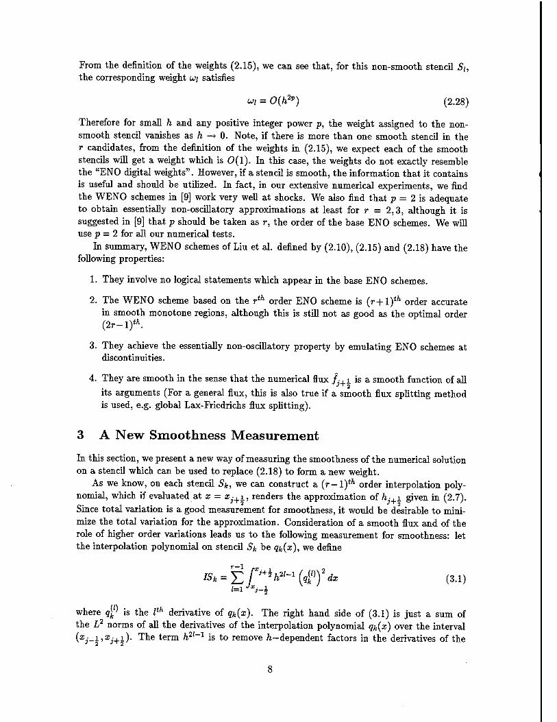
In this section, we present a new way of measuring the smoothness of the numerical solution on a stencil which can be used to replace (2.18) to form a new weight.

As we know, on each stencil Sk, we can construct a (r-l)th order interpolation poly- nomial, which if evaluated at x = Xj+i, renders the approximation of h-.i given in (2.7). Since total variation is a good measurement for smoothness, it would be desirable to mini- mize the total variation for the approximation. Consideration of a smooth flux and of the role of higher order variations leads us to the following measurement for smoothness: let the interpolation polynomial on stencil Sk be qk{x), we define

r_1 ~»h»-*(A*yd* (3.i) /=1 "'i-i

where q^' is the Ith derivative of qk{x). The right hand side of (3.1) is just a sum of the L2 norms of all the derivatives of the interpolation polynomial qk{x) over the interval (Xj_i,xj+i). The term h21'1 is to remove ^-dependent factors in the derivatives of the

J_i Jx

2

8

polynomials. This is similar to but smoother than the total variation measurement based on the Ll norm. It also renders a more accurate WENO scheme for the case r = 3, when used with (2.15) and (2.16).

When r = 2, (3.1) gives the same measurement as (2.18). However, they become different for r > 3. For r = 3, (3.1) gives

/So = ^(/i-2-2/i_1+/i)2 + ^(/j_2-4/j_1+3/i)

2 (3.2)

IS, = -(fj-i-2fj + fj+1f + -(fj_1-fj+lf (3.3)

IS2 = f(/i-2/i+1+/i+2)2 + i(3/i-4/i+1 + /j+2)2 (3.4)

In smooth regions. Taylor expansion of (3.2)-(3.4) gives, resp.

Bo = ^(f"h2)2 + \(2fh - lf'"h3)2 + 0{h&) (3.5)

ISi = ^(f'h2)2 + \{2fh + \f"h*)2 + 0(h6) (3.6)

IS2 = ^(f'h2)2 + \{2fh - |/'"/>3)2 + 0(h«) (3.7)

where /"' = f'"(uj). If /' ^ 0, then

ISk = (A)2(l + 0(h2)) k = 0,1,2 (3.8)

which means the weights (see (2.15)) resulting from this measurement satisfy (2.17) for r = 3, thus we obtain a 5th order (the optimal order for r = 3) accurate WENO scheme.

Moreover, this measurement is also more accurate at critical points of f(u(x)). When /' = 0, we have

ISk = ^(f"h2)2(l + 0(h2)) k = 0,1,2 (3.9)

which implies that the weights resulting from the measurement (3.1) are also 5th order accurate at critical points.

To illustrate the different behavior of the two measurements (i.e. (2.18) and (3.1)) for r = 3 in smooth monotone regions, near critical points or near discontinuities, we compute the weights k>0,u?i and w2 for the following function:

( smlTcxj if 0 < XJ < 0.5, . Jj \l- sin 2VXJ if 0.5 < Xj < 1. l U;

at all half grid points xJ+i where Xj = jAx, x-+i = Xj + Ax/2 and Arc = 1/40. We

display the weights o;o and u>i in Figure 1. (u;2 = 1 — u>0 — u, is omitted in the picture). Note the optimal weight for u>0 is CQ = 0.1 and for wx is Cf = 0.6. We can see that the weights computed with (2.18) (referred to as the original measurement in Figure 1) are far less optimal than those with the new measurement especially around the critical points x = |,|. However, near the discontinuity x = ^, the two measurements behave similarly: the discontinuous stencil always gets an almost zero weight. Moreover, for the grid point immediately to the left of the discontinuity, CJO

a 7 and u>j « |, which means, when only one of the three stencils is non-smooth, the other two stencils get 0(1) weights. Unfortunately,

Original Measurement oo0

Original Measurement OJ,

New Measurement a>0

New Measurement

0.25 0.50

ö^wo-oqloooao-o^i

0.75 1.00

Figure 1: A comparison of the two smoothness measurements.

these weights do not approximate a 4th order scheme at this point. A similar situation happens to the point just to the right of the discontinuity.

For simplicity of notations, we use WENO-X-3 to stand for the 3rd order WENO scheme (i.e. r = 2, for which the original and new smoothness measurement coincide) where X=LF, Roe, RF refers resp. to the global Lax-Friedrichs flux splitting, Roe's flux splitting and Roe's flux splitting with entropy fix; The accuracy of this scheme has been tested in [9]. We will use WENO-X-4 to represent the 4th order WENO scheme of Liu et al. (i.e. r = 3 with the original smoothness measurement of Liu et al.) and WENO-X-5 to stand for the 5th

order WENO scheme resulting from the new smoothness measurement. In later sections, we will also use ENO-X-Y to denote conventional ENO schemes of "Y"th order with "X" flux splitting. We caution the reader that the orders here are in L1 sense. So ENO-RF-4 in our notation refers to the same scheme as ENO-RF-3 in [15].

In the following we test the accuracy of WENO schemes on the linear equation:

ut + ux - 0 -1<£<1

u(x,0) = u0(x) periodic. (3.11)

(3.12)

In Table 3, we show the errors of the two schemes at t = 1 for the initial condition u0(x) = sin(xa;) and compare them with the errors of the bth order upstream central scheme (referred to as CENTRAL-5 in the following tables). We can see that WENO-RF-4 is more accurate than WENO-RF-5 on the coarsest grid (N=10) but becomes less accurate than WENO-RF- 5 on the finer grids. Moreover, WENO-RF-5 gives the expected order of accuracy starting at about 40 grid points. In this example and the one for Table 4, we have adjusted the time step to At ~ (Ax)* so that the 4th order Runge-Kutta in time is effectively 5th order.

In Table 4, we show errors for the initial condition u0(x) = sin4(^x). Again we see that WENO-RF-4 is more accurate than WENO-RF-5 on the coarsest grid (N=20) but becomes less accurate than WENO-RF-5 on finer grids. The order of accuracy for WENO settles

10

Table 3: Accuracy on ut + ux = 0 with UQ{X) = sin(7ra;).

Method N Loo error Loo order L\ error L\ order 10 1.31e-2 - 7.93e-3 - 20 3.00e-3 2.13 1.32e-3 2.59

WENO-RF-4 40 4.27e-4 2.81 1.56e-4 3.08 80 5.176-5 3.05 1.13e-5 3.79 160 4.99e-6 3.37 6.88e-7 4.04 320 3.44e-7 3.86 2.74e-8 4.65 10 2.98e-2 - 1.60e-2 - 20 1.45e-3 4.36 7.41e-4 4.43

WENO-RF-5 40 4.58e-5 4.99 2.22e-5 5.06 80 1.48e-6 4.95 6.91e-7 5.01 160 4.41e-8 5.07 2.17e-8 4.99 320 1.35e-9 5.03 6.79e-10 5.00 10 4.98e-3 - 3.07e-3 - 20 1.60e-4 4.96 9.92e-5 4.95

CENTRAL-5 40 5.03e-6 4.99 3.14e-6 4.98 80 1.57e-7 5.00 9.90e-8 4.99 160 4.91e-9 5.00 3.11e-9 4.99 320 1.53e-10 5.00 9.73e-ll 5.00

down later than in the previous example. Notice that this is the example for which ENO schemes lose their accuracy [12].

4 A Simple Way for Computing Weights for Euler Systems

For system (1.1) with d > 1, the derivatives J^,« = 1,.. .,d are approximated dimension

by dimension: for example, when approximating ^-, one fixes xi,l > 1 and uses an one dimensional approximation in the direction of x\. In the following, we only discuss how to approximate ^ and will drop the index "1" for simplicity. We will also assume that all

the eigenvalues of the Jacobian J£ are nonnegative (a condition identical to /' > 0 in the scalar equation). For a general flux, one can split it locally into positive and negative parts just as in the scalar case. The formulas for the negative part of the flux will be omitted due to symmetry.

For systems of equations, the fluxes f + i are usually approximated in the (local) char- acteristic fields. Let's take A-+i to be some average Jacobian at x-+i, e.g., the arithmetic

u=(ui+uJ+1)/2 (4.1)

mean

A*\ du

or for Euler systems, the Roe's mean matrix [11]. We denote by rs (column vector) and ls (row vector) the sth right and left eigenvector of A-+i, resp. Then the scalar WENO

11

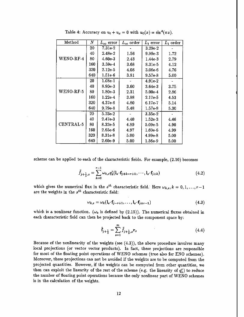
Table 4: Accuracy on ut + ux = 0 with u0(x) = sin4(7ra;).

Method N Loo error Loo order L\ error L\ order 20 7.31e-2 - 3.29e-2 - 40 2.48e-2 1.56 9.99e-3 1.72

WENO-RF-4 80 4.60e-3 2.43 1.44e-3 2.79 160 3.59e-4 3.68 8.31e-5 4.12 320 2.12e-5 4.08 3.06e-6 4.76 640 1.51e-6 3.81 9.57e-8 5.00 20 1.08e-l - 4.91e-2 - 40 8.90e-3 3.60 3.64e-3 3.75

WENO-RF-5 80 1.80e-3 2.31 5.00e-4 2.86 160 1.22e-4 3.88 2.17e-5 4.53 320 4.37e-6 4.80 6.17e-7 5.14 640 9.79e-8 5.48 1.57e-8 5.30 20 5.23e-2 - 3.35e-2 - 40 2.47e-3 4.40 1.52e-3 4.46

CENTRAL-5 80 8.32e-5 4.89 5.09e-5 4.90 160 2.65e-6 4.97 1.60e-6 4.99 320 8.31e-8 5.00 4.99e-8 5.00 640 2.60e-9 5.00 1.56e-9 5.00

scheme can be applied to each of the characteristic fields. For example, (2.10) becomes

r-l

U+\+ = X^ WM?3fc0«-fj+fc-r+l, • • *, ls-fj+fc) (4.2) k=0

which gives the numerical flux in the sth characteristic field. Here u>k,s,k = 0,1,...,r-l are the weights in the sth characteristic field:

">k,s — Wjfc(ls-fj_r+1,. . ., ls-fj+r—l) (4.3)

which is a nonlinear function, (uk is defined by (2.15)). The numerical fluxes obtained in each characteristic field can then be projected back to the component space by:

(4.4)

Because of the nonlinearity of the weights (see (4.3)), the above procedure involves many local projections (or vector vector products). In fact, these projections are responsible for most of the floating point operations of WENO schemes (true also for ENO schemes). Moreover, these projections can not be avoided if the weights are to be computed from the projected quantities. However, if the weights can be computed from other quantities, we then can exploit the linearity of the rest of the scheme (e.g. the linearity of qr

k) to reduce the number of floating point operations because the only nonlinear part of WENO schemes is in the calculation of the weights.

12

The question then is what quantities can serve as replacements of the projected val- ues. Obviously for each characteristic field, the replacing quantity must indicate the jump discontinuities in that field. Although such quantities are yet to be discovered for general systems of equations, we find, after an extensive searching and trial, that pressure and en- tropy are good replacements for the projected values when Euler systems are concerned, at least for problems without strong shocks and reflective waves.

Namely, we will use pressure to compute the weights in the genuinely nonlinear charac- teristic fields (s = l,m) and use entropy for the linearly degenerate field(s) (1 < s < m). The motivation: (1). The pressure does not jump at contact discontinuities but always jumps at shocks; (2). The entropy jumps at contact discontinuities but jumps only slightly at a weak shock.

Since the pressure and entropy can be obtained independent of the characteristic projec- tion procedure, we can reformulate the WENO schemes to take advantage of the linearity of the rest of the scheme. Let's define

r-l

^i+i',« = Yl w*,«?*(fi+*-r+i ,■■■■> tj+k) s = l,...,m (4.5) k=0

For Euler systems, the sth (1 < s < m) characteristic field is linearly degenerate. These fields have the same characteristic speed (eigenvalue) and the weights are all computed from the entropy. So we have for all 1 < s < m:

Uk,s=uk,2 Vfc = 0,...,r-1.

and therefore

for all 1 < s < m. Combine (4.2) and (4.4) and use the linearity of q\ to take out ls, we get

m

= (li <Fj+hl - ^+|,2)) ri + (M-Fi+i,m - ?i+iA)) *m + ?j+h2 (4.6)

As we can see, we only need two projections from component space to characteristic space and two inverse projections, plus the few operations for computing T>\ s,s = 1,2, m.

We will denote, by WEN0-LF-5-PS, the WENO scheme for the case r = 3, which uses pressure and entropy for weight computation in conjunction with the new smoothness measurement (3.1), the weights (2.15) and global Lax-Friedrichs flux splitting (according to our numerical tests, the original smoothness measurement of Liu et al. does not perform well at shocks when combined with the above way of computing weights).

Accuracy of WENO-LF-4, WENO-LF-5 and WEN0-LF-5-PS on the ID Euler system is tested using an initial condition which produces a smooth solution, the same example used in Section 6. The result is similar to the scalar case in Table 3 and thus will not be shown.

13

5 Sharpening of Contact Discontinuities

For a linear, constant coefficient problem ( f(u) = cm in (2.1)), Yang's artificial compression method, when applied to the WENO schemes is simply ( assuming c> 0 ):

ffH = fj+i + ci+i (5.1)

where /-+i is the flux obtained by one of the methods introduced in the previous three sections, and

S+l = m (5.2) ym(/£§ - /j+i>/£i - /,■-§)»/i+i - fj+^fjli - /i-i

Here f.x is obtained by the same method for /•_, i pretending a < 0; m is the usual J"r 2 2

minmod function defined by

f 5",W l°«'l' if« = «*5»(ai) = ••• = sign(an) m(a1,---,an) = < *<*<" (5.3)

^ 0 otherwise;

and aj is given by

""(^w^h)' (s-4) where a is a positive parameter. We will use a = 33 as suggested by Yang [20] in all our tests in Section 8, though this parameter can be tuned to optimize the results for individual problems. The case of a < 0 can be treated symmetrically and the generalization to variable coefficient or nonlinear problems is rather straight forward. See [15] for details.

We will apply the above sharpening technique only to contact discontinuities or contact characteristic field(s) in case of Euler systems. A scheme which uses the above artificial technique will be denoted by adding to its name the suffix "-A", e.g. WENO-LF-5-A.

6 Convergence for Smooth Solutions

As we can see from the previous sections, the WENO schemes are smooth in the sense that the spatial operator L

L — L{fj-r, fj-r+l,- ■ ■, fj+r-l) (6.1)

is infinitely differentiable to any of its arguments ( see (2.2), (2.10), (2.15), (2.16) and (2.18) or (3.1)). Here r > 2 is the L\ order of the base ENO scheme. In case of a general flux, if a smooth flux splitting is used (e.g. the global Lax-Friedrichs flux splitting), the smoothness of the WENO schemes is unchanged.

Strang's theorem (Theorem I in [18]) implies that, for a conservation law whose flux function and solution have enough continuous derivatives, a smooth, consistent scheme is convergent if its first variation (see [18] for the definition) is /2-stable.

It is easy to see that, for the scalar one dimensional conservation law (2.1) with /' > 0, the spatial operator of WENO schemes has the following simple first variation L

J+r-l QL

l=j—r

/'(%) Ax (^-lVj-r+l, * • •, tlj+r-l) " «^.iVi-r, ' ' ', Vj+r-lj) (6-2)

14

because §^(«j," -,UJ) = 0 and uk(uj,-•-,UJ) = Crk for all k = 0,...,r- 1 and I =

j - r,... ,j + r - 1. (6.2) can be rewritten into a summation of a (2r - 2)th order central difference D2r~2 and a (2r — l)i/l order upwind biased difference.

L = - Ax

(p2r-\uj.r+U- ■ •, tti+r_!) + (-l)'-1^^-1«^) (6.3)

where rr = 'r fcr-i)! > ^ an<^ ^+ * ^s t^ie (2r ~"1)*'1 order forward difference operator. Applying the classical Fourier analysis to the first variation, we see that the (2r — 2)th order central difference has a purely imaginary spectrum while the second term in (6.3), which is just a (2r — l)th order upwind biased difference, has a spectrum of the form

^-^H) 2r-1 9 6 (sin- + icos-) (6.4)

where 0 < 0 < 2ir. (6.3) and (6.4) together imply that the spectrum of the operator L lies fully on the left half of the complex plane. Therefore, with an appropriately chosen CFL number, the first variation of the WENO schemes are ^-stable when the 3rd or higher order Runge-Kutta time discretization is used.

Let's define by u(xo,to,Ax) the numerical solution at (x0,<o) € Rd x R+ for grid size Ax and fixed CFL number. For general scalar conservation laws, the same analysis gives

Theorem 6.1 For the initial value problem of (1.1) with m = 1 (i.e., scalar conservation laws), V(xo,<o) G RdxÄ+, if the exact solution v and ^,g have r+[^^]+q0+2 continuous derivatives in the domain of dependence of (xo,*o) as defined in [18], the WENO schemes using a smooth flux splitting and a nth order Runge-Kutta scheme ( n > max(r, 3) ) satisfy

ti(x0, t0, Ax) = v(xo, t0) + 0(Axr) (6.5)

for appropriately chosen CFL number. Here go is a small constant integer (see [18]).

For a few special cases, we list the CFL numbers in Table 5.

Table 5: CFL numbers (n: order of the Runge-Kutta scheme).

n = 3 n = 4 r = 2 1.625 1.745 r = 3 1.434 1.731

7 Efficiency Comparison

In this section, we compare the efficiency of WENO-LF-4, WENO-LF-5, WEN0-LF-5-PS and ENO-LF-4 on a vector supercomputer (CRAY C-90) and two serial workstations (SUN SparclO and SGI Indigo2).

15

ID, 2D and 3D Euler systems are solved. The 3D Euler system is (1.1) with d = 3, m = 5 and

u = (p,pu,pv,pw,E)T; (7.1)

f(u) = (pu,P + pv?,puv,puw,u(E + P))T; (7.2)

g(u) = (pv,pvu,P + pv2,pvw,v(E + P))T; (7.3)

h(u) = (pw,pwu,pwv,P + pw2,w(E +P))T. (7.4)

where

P = (7-l)(£-^,(«2 + *2 + ™2))

The initial condition is

p = 1 + 0.2 sin(7r(x + y + z)), u = v = w = 1, P = l

Here we use f, g, h, x, y, z instead of fa, f2, f3, Zi, x2, x3. The ID and 2D Euler systems and their initial conditions can be deduced from the above 3D problem by removing the extra degree of freedom(s).

We display the CPU time of ENO-LF-4, WENO-LF-4, WENO-LF-5 and WENO-LF- 5-PS (all with RK-4) on the CRAY C-90, the SparclO and the SGI Indigo2 in Table 6. We observe that WENO-LF-4 and WENO-LF-5 are at least twice as fast as ENO-LF-4 on the CRAY C-90 and WENO-LF-5-PS is 2.5 times as fast as ENO-LF-4 for the ID Euler problem, 3.2 times as fast for the 2D Euler problem and 3.9 times as fast for the 3D Euler system. On the workstations, WENO-LF-4 and WENO-LF-5 are a bit faster than ENO- LF-4 on the SUN SparclO but a bit slower on the SGI Indigo2. WENO-LF-5-PS is 1.5 to 2.2 times as fast as ENO-LF-4 on the SUN SparclO and on the SGI Indigo2. As a reference, we also include the CPU times of a typical second order TVD scheme [8] (Van Leer's limiter with 2nd order Runge-Kutta scheme in time, our own implementation) in the following tables. We can see the 2nd order scheme is about 10 times as fast as ENO-LF-4 on the CRAY C-90, 4.5 times as fast on the SUN SparclO and 3.5 times as fast on the SGI Indigo2.

In Table 7, the number of floating point operations and the MFlops (million floating- point operations per second) are given for the 2nd order scheme, ENO-Roe-4, ENO-LF-4, WENO-LF-5, WENO-LF-5-PS, ENO-Roe-4-A and WENO-LF-5-A. The operation count and MFlops for WENO-LF-4 is about the same as those for WENO-LF-5, thus omitted in the table. We can see all the WENO schemes achieve the speed of about 500 MFlops, which is 50% of the peak speed of CRAY C-90. The decrease of MFlops for high dimensions is because of the shorter array length N used in our tests. Notice also that the operation count per grid point per Runge-Kutta stage, of the full characteristic based 4th or 5th order ENO schemes using Lax-Friedrichs building blocks, is about 3 to 4 times that of the 2nd

order schemes. This ratio actually decreases to only about 1.5 if the Roe building block is used instead, i.e. f+(u) and f~(u) are not approximated separately. This is somewhat surprising, as it was commonly believed that high order methods are much more expensive than lower order ones. When the Roe building block is used, Yang's artificial compression causes a 40% increase in operation count for the ID Euler system and a 65% increase for the 2D Euler system as we can see from the operation counts for ENO-Roe-4 and ENO- Roe-4-A. When the Lax-Friedrichs building block is used, the increase of operation count is 65% for the ID Euler system and 100% for the 2D Euler system as shown by the operation

16

Table 6: CPU time in seconds. N points in each spatial dimension; 104-d iterations for the d-dimensional system.

d N 2nd order ENO-LF-4 WENO-LF-4 WENO-LF-5 WENO-LF-5-PS CRAY C-90, compiled with "-0 vector2"

1 1600 1.75 16.67 7.44 7.45 6.29 2 200 13.13 122.52 63.93 60.84 37.67 3 60 15.48 171.42 76.79 78.89 43.47

SUN SparclO (66MHz, HyperSparc), compiled with "-r8 -04" 1 1600 69.43 311.22 317.55 319.02 215.95 2 200 512.33 2582.25 2132.50 2116.53 1163.72 3 40 178.95 807.75 716.05 754.88 389.77

SGIIndigo2 (75MHz, R8000), compiled with "-r8 -03" 1 1600 21.03 66.21 73.88 77.01 58.14 2 200 151.26 555.51 564.54 578.22 347.48 3 60 167.44 626.92 699.58 715.91 366.29

counts for WENO-LF-5 and WENO-LF-5-A. The increase in CPU time is well reflected by the above percentages.

8 Numerical Results

8.1 Scalar Conservation Laws in One Dimension

Example 1. Linear Equation. We solve the linear equation:

ut + ux

u(a:,0)

0 -Kx < 1,

tto(z) periodic

where

u0(x) - <

' \ (G(x, ß,z-6) + G(x, ß,z+S) + 4G(x, ß, z)) -0.8 < x < -0.6; 1 -0.4 < x < -0.2; l-|10(as-0.1)| 0<x<0.2; I (F(x, a, a-6) + F(x, a, a+ 6) + 4F(x, a, a)) 0.4 < x < 0.6; 0 otherwise.

= p-ß{x-zf G(x,ß,z) = e-

F(x, a, a) = ymax(l - a2(x - a)2,0)

The constants are taken as c = 0.5, z = -0.7,6 = 0.005, a = 10 and ß = ^. The solution contains a smooth but narrow combination of Gaussians, a square wave, a sharp triangle wave, and a half ellipse.

We compute the solution up to t = 8 with 200 points. The results are shown in Figure 2. We observe that both WENO-Roe-4 and WENO-Roe-5 perform better than ENO-Roe-4

17

Table 7: Number of operations per Runge-Kutta stage per grid point and MFlops on CRAY C-90. d: the spatial dimension.

Scheme d x±y x *y x/y \x\ sign(x) xy,y/x- MFlops

2nd order 1 82 83 9 8 3 3 478 2 239 248 22 20 8 6 400 3 476 506 39 36 15 9 350

ENO-Roe-4 1 102 98 3 19 0 3 179 2 309 304 6 50 0 6 191 3 663 656 9 93 0 9 —

ENO-LF-4 1 244 233 3 39 0 3 223 2 791 766 6 102 0 6 219 3 1751 1718 9 189 0 9 190

WENO-LF-5 1 235 284 27 3 0 3 557 2 703 838 70 6 0 6 503 3 1466 1718 129 9 0 9 442

WENO-LF-5-PS 1 145 129 13 3 0 4 474 2 341 315 26 6 0 8 453 3 576 579 39 9 0 12 357

ENO-Roe-4-A 1 144 135 4 33 6 3 164 2 511 484 10 106 24 6 178

WENO-LF-5-A 1 375 447 37 19 12 3 526 2 1379 1654 110 70 48 6 482

18

for all the four types of waves in the initial condition. WENO-Roe-4 does better than WENO-Roe-5 at acute turns in the solution curve (or spike-like peaks) but WENO-Roe-5 does better for the square wave and at obtuse turns in the solution curve. With Yang's artificial compression technique, WENO-Roe-5-A performs the best at all waves. Note, we have adjusted the CFL number for WENO-Roe-5-A from 0.4 to 0.2. For CFL=0.4, using a = 40 in (5.4) gives similar results.

Example 2. Non-convex Problems. We test the 3rd and 5th order WENO schemes on the Buckley-Leverett problem whose flux is

*")= 4*+ (!-.)» <">

with initial data u = 1 in [|,0] and u = 0 elsewhere. (For the numerical results of the 4th

order WENO scheme of Liu et al., see [9]). The exact solution is a shock-rarefaction-contact discontinuity mixture.

The results obtained by WENO-RF-3 (with RK-3) and WENO-RF-5 (with RK-4) are shown in Figure 3. We can see both schemes converge to the correct entropy solution and give sharp shock profile. Note that, around discontinuities, WENO schemes are simulating the base ENO schemes. Therefore the sharpness of the shock profile obtained by the WENO schemes are only expected to be as good as that obtained by the base ENO schemes. However, in terms of this sharpness, our tests show that the 3rd order WENO scheme is comparable to the 3rd order ENO scheme instead of the base 2nd ENO scheme and, the 5th

WENO scheme is comparable to the 4th order ENO scheme.

8.2 Euler System in One Dimension

Example 1. ID Riemann Problems. We consider here two well known problem, which have the following Riemann type initial conditions:

u(x,0) =

The first one is the Sod problem [17]. The initial data are:

(pL,qL,PL) = (1,0,1); (pR,qR,PR) = (0.125,0,0.1)

The second one is the Riemann problem proposed by Lax [7]:

(pL, 9L, PL) = (0.445,0.698,3.528); (pR, qR, PR) = (0.5,0,0.571)

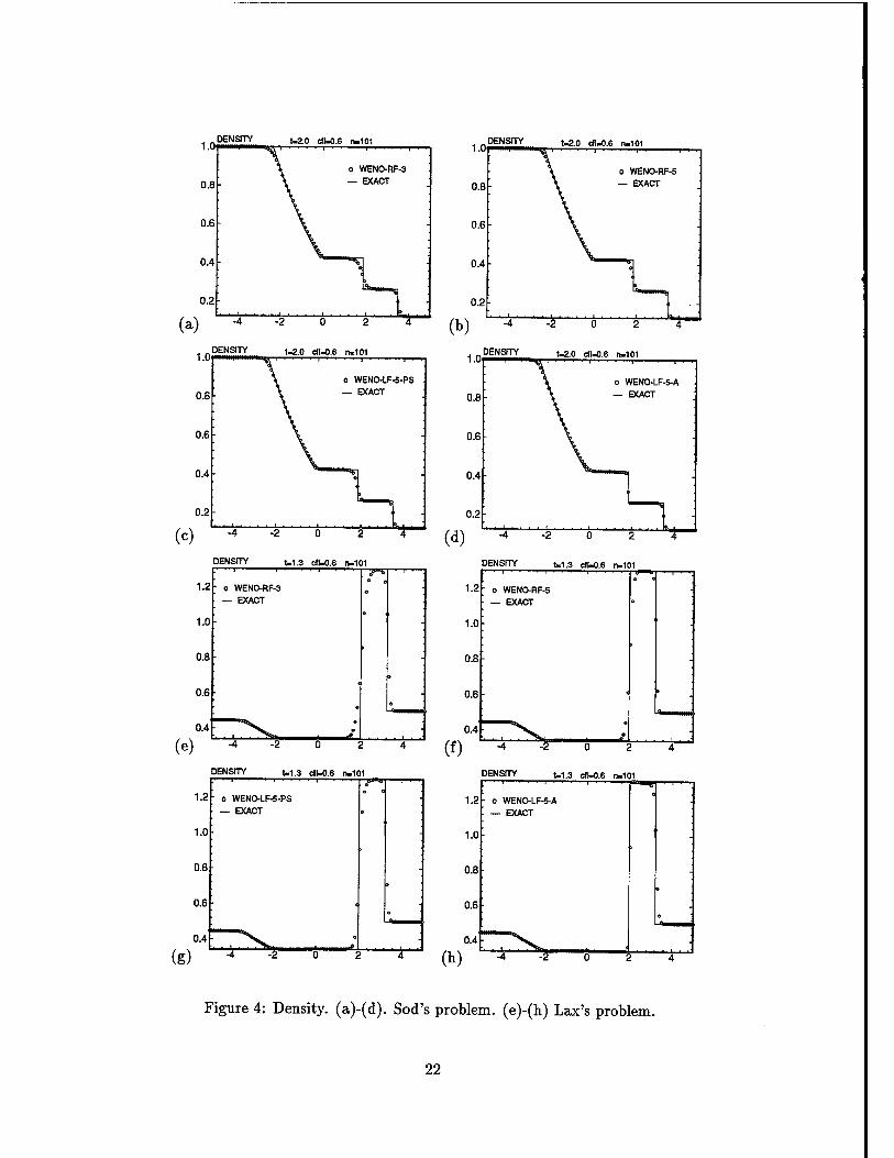
The numerical results are presented in Figure 4. We can see that all schemes give the correct solution with good resolution. WENO-RF-5 is better than WENO-LF-5-PS which is in turn better than WENO-RF-3. We note that Figures 4b and 4c ( Figures 4e and 4f) are comparable, resp. to Figure 10 ( Figure 11) in [15]. Also see Figures 9a ( Figure 10a) in [9]. WENO-LF-5-A does much better than all other schemes at the contact discontinuities. We would like to point out that, according to our experience with extensive numerical testing, these two problems, especially the Lax's problem, are tough test cases for non-characteristic

19

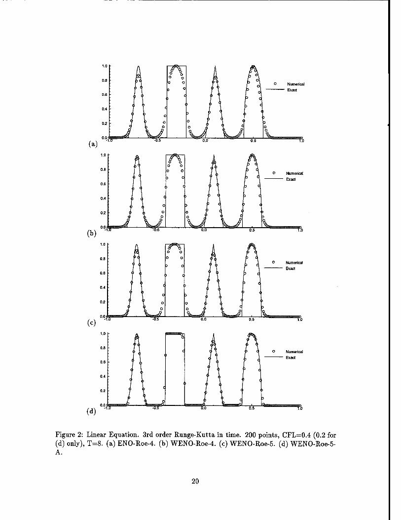
Figure 2: Linear Equation. 3rd order Runge-Kutta in time. 200 points, CFL=0.4 (0.2 for (d) only), T=8. (a) ENO-Roe-4. (b) WENO-Roe-4. (c) WENO-Roe-5. (d) WENO-Roe-5- A.

20

t.0.4 cfl-0.8 n-81

(»)•*> 0>)'

1.0

0.8

0.6

0.4-

02

t-0.4 dl-0.8 n-81

0 WENO-RF-5

— EXACT

0.5 10

Figure 3: The Buckley-Leverett problem, (a): WENO-RF-3; (b): WENO-RF-5.

based schemes of order at least three. Oscillations can easily appear for such schemes. Here WENO-LF-5-PS performs well in these two cases.

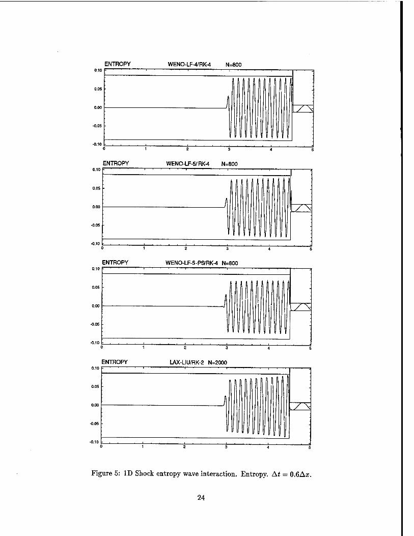
Example 2. ID Shock Entropy Wave Interaction. In this example, we test the WENO schemes on a model that involves a moving shock interacting with an entropy wave of small amplitude. On a domain [0,5], the initial condition is:

p = 3.85714; u = 2.629369; P = 10.33333; when x < 0.5 p = e-csm(kx). U = Q. p = 1. when a;>0.5

where e and k are the amplitude and wave number of the entropy wave, resp. The mean flow is a pure right moving Mach 3 shock. If € is small compared to the shock strength, the shock will march to the right at approximately the non-perturbed shock speed and generate a sound wave which travels along with the flow behind the shock. At the same time, the perturbing entropy wave, after "going through" the shock, is compressed and amplified and travels approximately at the speed of u + c where u and c are the velocity and speed of the sound of the mean flow left of the shock. The amplification factor for the entropy wave can be obtained by linear analysis. See [10, 21] for details. In order to get rid of the transient waves due to the non-numerical initial shock profile, we let the shock move up to x = 4.5 and then shuffle it back to x = 0.5. The solution is examined when the shock reaches x = 4.5 the second time.

The goal of this test is to examine the stability and accuracy of the WENO schemes in the presence of the shock. Since the entropy wave here is set to be very weak relative to the shock, any excessive oscillation could pollute the generated waves (e.g. the sound waves) and the amplified entropy waves. In our tests, we take e = 0.01 and k = 13. The amplitude of the amplified entropy waves predicted by the linear analysis is 0.08690716 (shown in the following figures as horizontal solid lines). First we use 800 points which is effectively 20 points in each wave length of the generated entropy wave. Since the generated sound waves (or pressure wave) are of lower frequency than the amplified entropy waves, they are much better resolved by this grid size. Therefore we only display the entropy component of the numerical solutions. WENO-LF-4, WENO-LF-5 and WENO-LF-5-PS are used in our tests and the results are shown in Figure 5 (the mean flow has been subtracted from

21

(a)

1.0 DENSITY t-2.0 cfl-0.6 n-101

\ o WENO-RF-3

0.8 V — EXACT

0.6 ■ \

0.4 ©

0.2

> h - -4 -2 0 2 4

(c)

1.0 DENSITY t-2.o cfl-0.6 n-101

t t '

o WENO-LF-5-PS

0.8 ■

— EXACT

0.6 -

0.4 0 •

)

0.2 • -4 -2 0 2

!„.,.„

DENSITY U1.3 cfU0.6 n-101

1.2 • o WENO-RF-3 — EXACT

1.0

0.8

0.6-

(e)

7°T

-4-2 0

DENSITY t.1.3 cfl-0.6 n.101

(g)

1.2 ■ o WENO-LF-5-PS — EXACT

© 0

1.0

» '

0.6 9

0.6 ( e

0.4 e - -4 -2 6 ) 4

0>)

DENSITY t-2.0 cfl-0.6 n-101

o WENO-RF-5

0.8 — EXACT

0.6 ■ ■

U.4

> 0.2 -

-4 -2 0 2 4

(d)

1.0 DENSITY t-2.0 cfl-0.6 n-101

""^J 1

o WENaLF-5-A

0.8 - — EXACT

0.6

0.4 i .

0.2 ■

-4 -2 0 2 J

CO

DENSfTY U1.3 cfl-0.6 n-101

© <

1.2 ■ o WENO-RF-5 - — EXACT °

1.0

■ » -

0.8 "

0.6 < *

0.4 " -4-2 0 2 ) 4

DENSfTY t-1.3 cfl-0.6 n-101

W

1.2 • o WENO-LF-5-A — EXACT

0

1.0

0.8 -

0.6

9

©

0.4

-4 -2 0 s ) 4

Figure 4: Density, (a)-(d). Sod's problem, (e)-(h) Lax's problem.

22

the numerical solution). We see that all three schemes catch the amplified entropy waves quite well. WENO-LF-4 performs the best on this grid and WENO-LF-5 ranks the second. In order to examine the relative performance of WENO-LF-4 and WENO-LF-5, we run the same test on a grid of 1200 points. The results for these two schemes are displayed in Figure 6. We can see that on this grid (approximately 30 points per wave length), WENO- LF-5 is as accurate as WENO-LF-4. In fact, on finer grids, WENO-LF-5 becomes more accurate than WENO-LF-4. This is in good agreement with our accuracy test in section 4. For the purpose of comparison with low order schemes, we also include the entropy computed by a typical second order scheme [8] (half Van Leer's limiter, half Superbee limiter with 2nd order Runge-Kutta scheme in time, 2000 points). The advantage of using higher order schemes for this example is apparent.

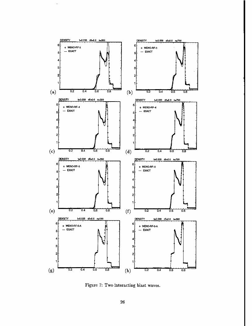
Example 3. Two Interacting Blast Waves. We consider here the interaction of two blast waves. The initial data are the following:

u(x,0) =

where

uL if 0 < x < 0.1 uM if O.K x < 0.9 UR if 0.9 < x < 1

PL = PM = PR = l UL = UM = UR = 0 PL = 103 PM = 10"2 PR = 102

A reflective boundary condition is applied at both x = 0 and x = 1. See [19] for a detailed discussion of this problem.

Three grids are used: 199, 399, 799 points. We examine our numerical solutions at t = 0.038. The "exact" solution (solid lines in all the pictures) are computed by ENO-RF-5 with 1600 points. In Figure 7, we show the density computed by WENO-RF-3 (with RK-3), WENO-RF-4, WENO-RF-5 and WENO-RF-5-A (with RK-4).

We observe that the 4th order and 5th order WENO schemes are much better than the 3rd order WENO scheme and the results are comparable with those obtained by the unmodified ENO-RF-4 (see Figure 12 in [15]. Note, the 4th order ENO scheme in the L1

norm was denoted as ENO-RF-3 there). WENO-RF-4 is slightly better than WENO-RF-5 on the medium grid while on the fine grid WENO-RF-5 seems to be better. The results of WENO-RF-5-A on the coarse and medium grids are nearly as good as WENO-RF-5 on, resp. medium and fine grids.

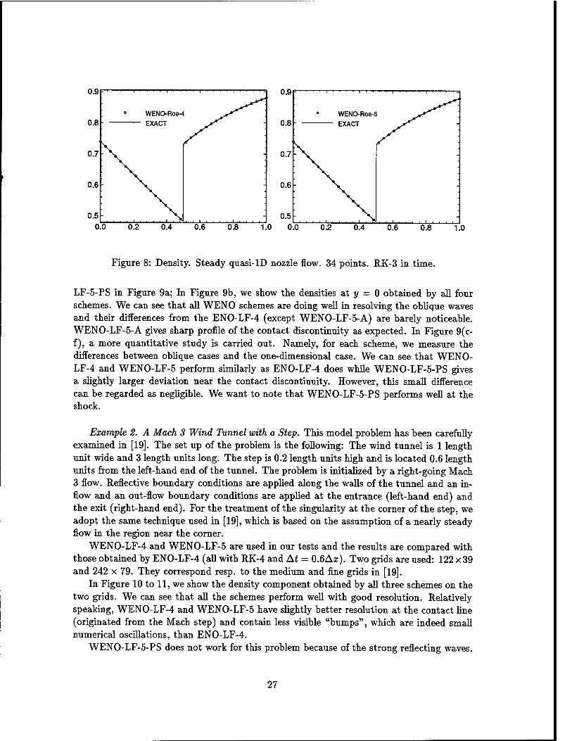
Example 4- Quasi-One Dimensional Nozzle Flow. In this example, we use the WENO schemes to solve the steady state quasi-lD nozzle flow. The governing equation of the quasi-lD nozzle flow is the ID Euler system with the following forcing term:

g(u, x) = -^-(pu, pu\ u(E + P)f

where A = A(x) is the cross area function of the nozzle and Ax = j£. The nozzle here is of unit length, whose shape is determined by assuming a linear, isentropic Mach number distribution, which is 0.8 at x = 0 (the entrance) and 1.8 at x = 1 (the exit). The exit flow condition is then decided by the prescribed shock position, which is x = 0.5 in our test.

In Figure 8, we display the density computed by WENO-Roe-4 and WENO-Roe-5 with 34 points. We can see both schemes converge nicely to the exact solution (solid line in the

23

ENTROPY 0.10

0.05

0.00

WENO-LF-4/RK-4 N=800

ENTROPY 0.10 F—'—'—"~

-o.os

UA

2 3

WENO-LF-5/RK-4 N=800

II

II

II

Z5

ZN

ENTROPY 0.10

WENO-LF-5-PSmK-4 N=800

ENTROPY LAX-LIU/RK-2 N=2000

o.os

-0.05

-0.10

zz^

Figure 5: ID Shock entropy wave interaction. Entropy. Ai = 0.6Ax.

24

ENTROPY WENO-LF-4/RK-4 N=1200 0.10 • , . * —. ■ 3

0.05 AAIAAI

I HUH

v\

111 -0.05 111 : -0.10 ..... i i , ,

ENTROPY WENO-LF-5/RK-4 N=1200 0.10 i i i - ■ - ' 1 ' ' • ' 2

0.05 min 111 ' ./\

iiiii -0.05 llllll : -010 i ...... , ,

Figure 6: ID Shock entropy wave interaction(cont'd). Entropy. At = 0.6Aa:.

pictures). The residue computed with both schemes settles down to 10~7 for this grid, and to a smaller number for a finer grid.

This example shows that WENO has its advantage for steady state calculations.

8.3 Euler System in Two Dimensions

Example 1. Oblique Sod's Problem. The purpose of this test is to analyze the capability of WENO schemes in resolving waves that are oblique to the computational mesh. The 2D Sod's problem is solved where the initial jump makes an angle 0 against the z-axis (0 < 0 < \). If 9 = -|, we have the one-dimensional Sod's problem. If 0 < 0 < -f, all the waves produced will be oblique to the rectangular computational mesh. We take our computational domain to be [0,6] x [0,1] and position the initial jump at (x, y) = (2.25,0). The physical domain varies with 0 and is taken as [0,^] x [0,^-g]. The scaling factor -^g is to ensure the same grid resolution normal to the wave propagation on a given mesh at some fixed time for all choices of 0. See [3] for details. We take 0 to be arctan 1, arctan2, and arctan 4. The solution is computed up to t = 1.2 on a 96 x 16 mesh.

WENO-LF-4, WENO-LF-5, WENO-LF-5-A and WENO-LF-5-PS are used in our tests and the results are compared with that obtained by ENO-LF-4 (all with RK-4 and At = 0.6Ax). For the case 0 — arctan 1, we display the density contours obtained by WENO-

25

DENSITY t-0.038 cfl.0.6 lta399

(a)

o WENO-RF-3

— EXACT T

0.2 0.4 0.6 0.8

DENSITY U0.038 cfl.0.6 n-399

DENSITY t-0.038 cfW.6 n-399

(e)

o WENO-RF-5

— EXACT

0.2 0.4 0.6 0.8

DENSITY W0.038 cfl-0.6 n-199

6

5

4

3

2|-

1

(g)

o WENO-RF-5-A

— EXACT

0.2 0.4 0.6 0.8

DENSITY t-0.038 cfl-0.6 n-799

DENSITY U0.038 cfU0.6 n-799

(d)

o WENO-RF-4

— EXACT

N 0.2 0.4 0.6 0.8

DENSITY U0.038 cfl-0.6 n-799

(f)

o WENO-RF-5

— EXACT

N /

0.2 0.4 0.6 0.8

00

DENSITY t-0.038 cfl-0.6 n-399

6

5

o WENO-RF-5-A

'_ — EXACT

•

4 ; \ -

3 X .

2 f 1 * 4_

0.2 0.4 0.6 0.8

Figure 7: Two interacting blast waves.

26

0.0 0.2 0.4 0.6 0.8 1.0 0.0 0.2 0.4 0.6 0.8 1.0

Figure 8: Density. Steady quasi-lD nozzle flow. 34 points. RK-3 in time.

LF-5-PS in Figure 9a; In Figure 9b, we show the densities at y = 0 obtained by all four schemes. We can see that all WENO schemes are doing well in resolving the oblique waves and their differences from the ENO-LF-4 (except WENO-LF-5-A) are barely noticeable. WENO-LF-5-A gives sharp profile of the contact discontinuity as expected. In Figure 9(c- f), a more quantitative study is carried out. Namely, for each scheme, we measure the differences between oblique cases and the one-dimensional case. We can see that WENO- LF-4 and WENO-LF-5 perform similarly as ENO-LF-4 does while WENO-LF-5-PS gives a slightly larger deviation near the contact discontinuity. However, this small difference can be regarded as negligible. We want to note that WENO-LF-5-PS performs well at the shock.

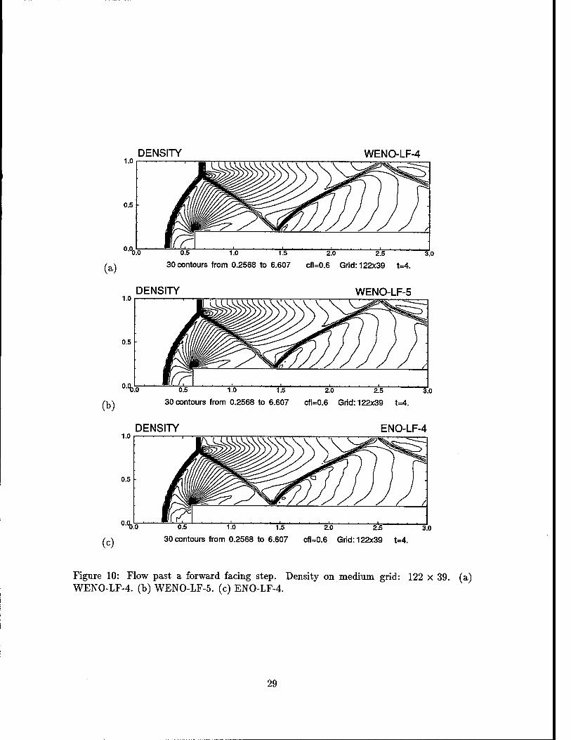
Example 2. A Mach 3 Wind Tunnel with a Step. This model problem has been carefully examined in [19]. The set up of the problem is the following: The wind tunnel is 1 length unit wide and 3 length units long. The step is 0.2 length units high and is located 0.6 length units from the left-hand end of the tunnel. The problem is initialized by a right-going Mach 3 flow. Reflective boundary conditions are applied along the walls of the tunnel and an in- flow and an out-flow boundary conditions are applied at the entrance (left-hand end) and the exit (right-hand end). For the treatment of the singularity at the corner of the step, we adopt the same technique used in [19], which is based on the assumption of a nearly steady flow in the region near the corner.

WENO-LF-4 and WENO-LF-5 are used in our tests and the results are compared with those obtained by ENO-LF-4 (all with RK-4 and At = 0.6Az). Two grids are used: 122 x 39 and 242 x 79. They correspond resp. to the medium and fine grids in [19].

In Figure 10 to 11, we show the density component obtained by all three schemes on the two grids. We can see that all the schemes perform well with good resolution. Relatively speaking, WENO-LF-4 and WENO-LF-5 have slightly better resolution at the contact line (originated from the Mach step) and contain less visible "bumps", which are indeed small numerical oscillations, than ENO-LF-4.

WENO-LF-5-PS does not work for this problem because of the strong reflecting waves.

27

1 .u

0.9 ':

0.8 ':

0.7

0.6

0.5

0.4

0.3

0.2

(b)

(c)

0.03

0.02

0.01

0.00

-0.01

-0.02

-0.03(

0.03

0.02

0.01

0.00

-0.01

-0.02

-0.03,

ENO-LF-4

WENO-LF-4

WENO-LF-5

WENO-LF-5-PS

WENO-LF-5-A

arctan 1

arctan 2

arctan 4

0.03

0.02

0.01

0.00

-0.01

-0.02

-0.03,

arctan 1

arctan 2

arctan 4

(d)

\ : araan 1

'TXP- YJ Si

* i

0.03

0.02

0.01

0.00

-0.01

-0.02

-0.03,

arctan 1

arctan 2

arctan 4

(e) (f)

Figure 9: Oblique Sod's problem, (a) Density contours. WENO-LF-5-PS, 9 = arctan 1. (b) Density, y = 0, 9 = arctan 1. (c)-(f) pe - p1D, y = 0. (c) ENO-LF-4. (d) WENO-LF-4. (e) WENO-LF-5. (f) WENO-LF-5-PS.

28

DENSITY WENO-LF-4

(a)

0.5 1.0 1.5 2.0 ^Z5 3 0

30 contours from 0.2568 to 6.607 cfl=0.6 Grid: 122x39 t=4.

DENSITY WENO-LF-5

(b)

0.5 1.0 1.5 2.0 2.5 3.0

30 contours from 0.2568 to 6.607 cfl=0.6 Grid: 122x39 t=4.

DENSITY ENO-LF-4

(c)

0.5 1.0 1.5 2.0 2.5 3 0

30 contours from 0.2568 to 6.607 cfl=0.6 Grid: 122x39 t=4.

Figure 10: Flow past a forward facing step. Density on medium grid: 122 x 39. (a) WENO-LF-4. (b) WENO-LF-5. (c) ENO-LF-4.

29

DENSITY WENO-LF-4

(a) 0.5 1.0 1.5 2.0 2.5 3 0

30 contours from 0.2568 to 6.607 cfl=0.6 Grid: 242x79 t=4.

DENSITY WENO-LF-5

00 0.5 1.0 1.5 2.0 2.5 3 0

30 contours from 0.2568 to 6.607 cfl=0.6 Grid: 242x79 t=4.

DENSITY ENO-LF-4

(c)

0.5 1.0 1.5 2.0 2.5 3 0

30 contours from 0.2568 to 6.607 cfl=0.6 Grid: 242x79 t=4.

Figure 11: Flow past a forward facing step (cont'd). Density on fine grid: 242 x 79. (a) WENO-LF-4. (b) WENO-LF-5. (c) ENO-LF-4.

30

Example 3. Double Mach Reflection of a Strong Shock. The computational domain for this problem is chosen to be [0,4] x [0,1]. The reflecting wall lies at the bottom of the computational domain starting from x = |. Initially a right-moving Mach 10 shock is positioned at x = |, y = 0 and makes a 60° angle with the x-axis. For the bottom boundary, the exact post-shock condition is imposed for the part from x = 0 to x = | and a reflective boundary condition is used for the rest. At the top boundary of our computational domain, the flow values are set to describe the exact motion of the Mach 10 shock. See [19] for a detailed description of this problem.

Two grids have been used in our tests: 240 x 59 and 480 x 119. They correspond to the medium and fine grids in [19], resp. We will only show the solutions on part of the domain: [0,3] x [0,1] where most of the flow features are located.

We use WENO-LF-4, WENO-LF-5 and ENO-LF-4 (all with RK-3 and At = 0.6Ax) in our tests. We show the density contours obtained by these three schemes. See Figure 12 and 13. We see that all three schemes resolve the two Mach stems well. Again WENO-LF- 5-PS does not work because of the strong reflecting wave pattern in this problem.

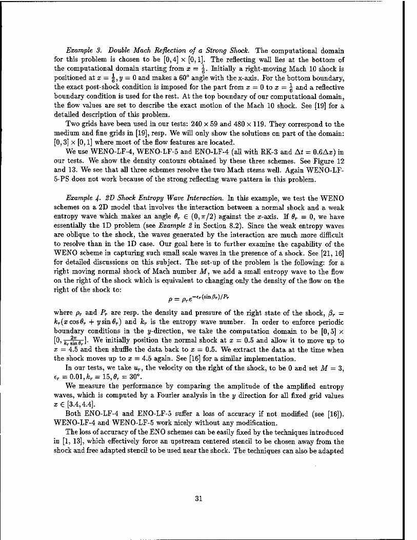
Example 4- 2D Shock Entropy Wave Interaction. In this example, we test the WENO schemes on a 2D model that involves the interaction between a normal shock and a weak entropy wave which makes an angle 6T € (0,7r/2) against the x-axis. If 9T = 0, we have essentially the ID problem (see Example 2 in Section 8.2). Since the weak entropy waves are oblique to the shock, the waves generated by the interaction are much more difficult to resolve than in the ID case. Our goal here is to further examine the capability of the WENO scheme in capturing such small scale waves in the presence of a shock. See [21, 16] for detailed discussions on this subject. The set-up of the problem is the following: for a right moving normal shock of Mach number M, we add a small entropy wave to the flow on the right of the shock which is equivalent to changing only the density of the flow on the right of the shock to:

p = Pre-er(siaßrVPr

where pT and Pr are resp. the density and pressure of the right state of the shock, ßr = kT(xcos6T + ysm0T) and kr is the entropy wave number. In order to enforce periodic boundary conditions in the t/-direction, we take the computation domain to be [0,5] x [0, k ^e ]. We initially position the normal shock at x — 0.5 and allow it to move up to x = 4.5 and then shuffle the data back to x = 0.5. We extract the data at the time when the shock moves up to x = 4.5 again. See [16] for a similar implementation.

In our tests, we take ur, the velocity on the right of the shock, to be 0 and set M = 3, er = 0.01,fcr= 15,0r = 3O°.

We measure the performance by comparing the amplitude of the amplified entropy waves, which is computed by a Fourier analysis in the y direction for all fixed grid values x£ [3.4,4.4].

Both ENO-LF-4 and ENO-LF-5 suffer a loss of accuracy if not modified (see [16]). WENO-LF-4 and WENO-LF-5 work nicely without any modification.

The loss of accuracy of the ENO schemes can be easily fixed by the techniques introduced in [1, 13], which effectively force an upstream centered stencil to be chosen away from the shock and free adapted stencil to be used near the shock. The techniques can also be adapted

31

DENSITY WENO-LF-4

0.0 0.5 1.0 1.5 2.0 2.5 3.0

(a) 30 contours from 1.731 to 20.92 Grid: 240x59 cfl=0.6 t=0.2

DENSITY WENO-LF-5

0.0 0.5 1.0 1.5 2.0 2!5 3.0

(b) 30 contours from 1.731 to 20.92 Grid: 240x59 cfl=0.6 t=0.2

DENSITY ENO-LF-4

0.0 0.5 1.0 1.5 2.0 2.5 3.0

(c) 30 contours from 1.731 to 20.92 Grid: 240x59 cfl=0.6 t=0.2

Figure 12: Double Mach reflection. Density on medium grid: 240 x 59. (a) WENO-LF-4. (b) WENO-LF-5. (c) ENO-LF-4.

32

DENSITY WENO-LF-4

0.0 0.5 1.0 1.5 2.0 2.5 3.0

(a) 30 contours from 1.731 to 20.92 Grid: 480x119 cfl=0.6 t=0.2

DENSITY WENO-LF-5

0.0 0.5 1.0 1.5 2.0 2.5 3.0

fl,) 30 contours from 1.731 to 20.92 Grid: 480x119 cfl=0.6 t=0.2

DENSITY ENO-LF-4

0.0 0.5 1.0 1.5 2.0 2.5 3.0

(c\ 30 contours from 1.731 to 20.92 Grid: 480x119 cfl=0.6 t=0.2

Figure 13: Double Mach reflection (cont'd). Density on fine grid: 480 x 119. (a) WENO- LF-4. (b) WENO-LF-5. (c) ENO-LF-4.

33

to enhance the performance of WENO schemes by modifying the weights as follows:

~)={Crk if JS^cT1 for any/= 0,...,r-l,

1 u>k otherwise. ^ ' '

where a is taken as 2 and vk,k = 0,...,r-l are the regularly computed weights. (8.2) leads to the optimal weights being used for stencils away from the shock and regularly computed weights being used near the shock. We denote the modified ENO-LF-4, ENO- LF-5, WENO-LF-4 and WENO-LF-5 to be, resp. EN02-LF-4, EN02-LF-5, WEN02-LF-4 and WEN02-LF-5. Note that, with the modified weights, WENO-LF-4 becomes 5th order accurate in smooth regions. In all tests, RK-4 is used with At = 0.6Aa:.

First we use 800 points in the z-direction and 20 points in the y—direction which give approximately 20 points per entropy wave length in both directions. In Figure 14, the amplitude of the amplified entropy waves obtained by all aforementioned schemes are displayed. The solid horizontal line is the amplitude predicted by linear analysis which is 0.08744786 (see [10, 21]). We see that the modified schemes generally perform better in terms of accuracy and decay rate than the unmodified schemes. As a reference, we have also included the amplitudes obtained by a typical second order TVD scheme [8] (half Van Leer's limiter, half Superbee limiter with 2nd order Runge-Kutta scheme in time, 800 points). We can see that high order schemes perform much better than the second order schemes in terms of accuracy and decay rate for this problem.

WENO-LF-5-PS does not perform well for this problem even with the remedy above. This indicates that the pressure-entropy combination is not good enough to indicate pre- cisely the smoothness of the numerical solution. This causes oscillations generated at shocks and thus destroys the accuracy of the scheme in resolving the waves which have "undergone" the interaction with the shock.

Remark: We have seen that WENO-LF-5-PS does not work for the step problem and the double Mach reflection problem because it can not handle the reflective boundary properly. This can be explained by the following: the usual way of imposing the reflective boundary condition3 is to reverse the normal velocity at the grid points which are symmetric with respect to that boundary while setting other flow quantities (density, pressure and tangential velocity) to be the same; in particular the pressure and entropy at each pair of symmetric grid points are identical. Therefore neither the pressure nor the entropy can indicate possible jumps in the normal velocity. This failure will result in an unstable weight distribution in the normal direction near the reflective boundary and cause fatal errors such as density becoming negative. An immediate "fix" seems to be using the normal velocity to compute the weights for one of the linearly degenerate fields. Unfortunately, the jump in the normal velocity is not like a contact discontinuity, which belongs solely to one of the characteristic fields. While this might cure the ill distribution of the weights in the field, in which the velocity is used, it can not cure this ill distribution in other fields.

However, WENO-LF-5-PS can be applied to problems where the reflective boundary does not play a vital role. As an example, we look at the following model problem.

Example 5. Shock Vortex Interaction. This model problem describes the interaction between a stationary shock and a vortex. The computational domain is taken to be [0,2] x

We assume here the physical boundary is flat, as is the case in aforementioned problems

34

0.087

0.077

0.067 -

0.057

0.047

0.037

0.027

0.017

LINEAR THEORY EN02-LF-4 EN02-LF-5 WEN02-LF-4 WENOJ

S-LF-4 WENO-LF-5

0 typical 2nd Order

3.4 4.4

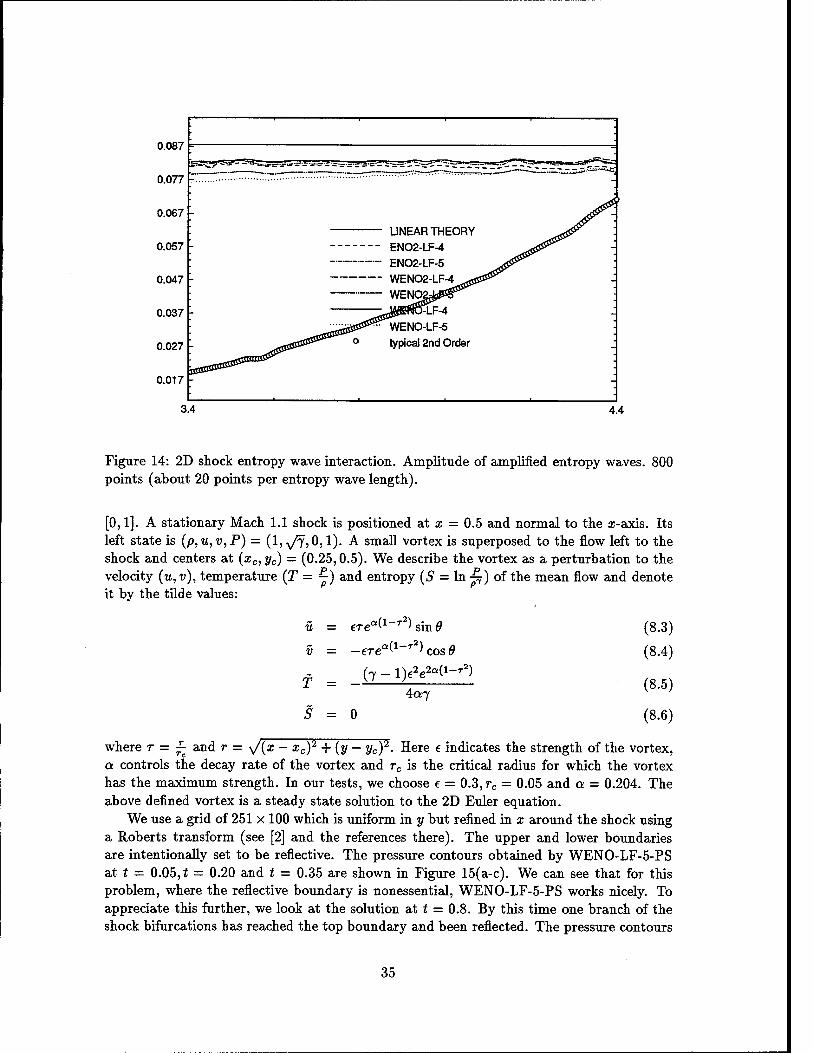
Figure 14: 2D shock entropy wave interaction. Amplitude of amplified entropy waves. 800 points (about 20 points per entropy wave length).

[0,1]. A stationary Mach 1.1 shock is positioned at x = 0.5 and normal to the z-axis. Its left state is (p, u, v, P) = (1, yfy, 0,1). A small vortex is superposed to the flow left to the shock and centers at (xc,yc) = (0.25,0.5). We describe the vortex as a perturbation to the velocity (u, v), temperature (T = j) and entropy (5 = In £) of the mean flow and denote it by the tilde values:

u

v

f

S

trea(l-r2)sinö

-ere^-^cosfl

(7 - l)e2e2a^-^) 4aj

= 0

(8.3)

(8.4)

(8.5)

(8.6)

where r = -^ and r = s/(x - xc)2 + (y - yc)

2. Here e indicates the strength of the vortex, a controls the decay rate of the vortex and rc is the critical radius for which the vortex has the maximum strength. In our tests, we choose 6 = 0.3, rc = 0.05 and a = 0.204. The above defined vortex is a steady state solution to the 2D Euler equation.

We use a grid of 251 x 100 which is uniform in y but refined in x around the shock using a Roberts transform (see [2] and the references there). The upper and lower boundaries are intentionally set to be reflective. The pressure contours obtained by WENO-LF-5-PS at t = 0.05, t = 0.20 and t = 0.35 are shown in Figure 15(a-c). We can see that for this problem, where the reflective boundary is nonessential, WENO-LF-5-PS works nicely. To appreciate this further, we look at the solution at t = 0.8. By this time one branch of the shock bifurcations has reached the top boundary and been reflected. The pressure contours

35

obtained by WENO-LF-5-PS at this moment are shown in Figure 15d. We see that the reflection is well captured.

In Figure 15(e-g), we compare the results obtained by WENO-LF-5-PS, WENO-LF- 5 and ENO-LF-4. 90 contours are drawn for the pressure component in the range of (1.19,1.37). We see that the three methods give approximately the same resolution. A careful examination reveals that WENO schemes are slightly better in the sense that less numerical noise is generated. Between the two WENO schemes, WENO-LF-5 seems a little better for the same reason. For a qualitative comparison, see also [2]. Note that a different vortex is used there.

Figure 15: 2D shock vortex interaction. Pressure, (a)-(d) WENO-LF-5-PS. 30 contours, (a) t=0.05. (b) t=0.20. (c) t=0.35. (d) t=0.80. (e)-(g) t=0.60. 90 contours from 1.19 to 1.37. (e) WENO-LF-5-PS. (f) WENO-LF-5. (g) ENO-LF-4.

Example 6. Flow Past a Cylinder. In this test, we use the WENO schemes to simulate

36

the supersonic flow past a cylinder. In the physical space, a cylinder of unit radius is positioned at the origin on a x — y plane. The computational domain is chosen to be [0,1] x [0,1] on the £-77 plane. The mapping between the computational domain and the physical domain is:

x = (Rx-(Rx-l)Z)cos(e(2V-l)) (8.7)

y = (Ry-(Ry-l)t)wL(6(2Ti-l)) (8.8)

where we take Rx = 3, Ry = 6 and 0 = ff. See [16] for the eigenvalues and eigenvectors of 2D Euler systems on general structured grids. A uniform mesh of 60 x 80 in the computational domain is used. For an illustration of the mesh in the physical space (drawing every other grid line), see Figure 16a.

The problem is initialized by a Mach 3 shock moving toward the cylinder from the left. A reflective boundary condition is imposed at the surface of the cylinder, i.e. £ = 1, inflow boundary condition is applied at £ = 0 and outflow boundary condition is applied at 17 = 0,1,

The pressure contour obtained by WENO-LF-5 with RK-4 and At = 0.6Ax is shown in Figure 16b. Similar results can be obtained by WENO-LF-4 and ENO-LF-4.

9 Conclusion

With the new smooth measurement, which is based on minimizing the L2 norm of the derivatives of the interpolation polynomials, the WENO schemes formulated from the rth

order ENO schemes can be made {2r-\)ih order accurate in smooth regions of the flux function (in spatial variables), at least for r = 2,3. However, at discontinuities, all WENO schemes are just rth accurate (r is the order of the base ENO scheme).

The 4th order WENO scheme of Liu et al. and the 5th order WENO scheme resulting from the new smoothness measurement are found to be at least twice as fast as the 4th order ENO schemes on vector supercomputers (e.g. CRAY C-90) and as fast on serial machines (therefore on parallel machines as well). Many ID and 2D numerical tests suggest that both WENO schemes are very robust for shock calculations. The 4th order WENO scheme of Liu et al. is slightly more accurate than the 5th order WENO scheme on coarse grids (20 points or less per wave length) but becomes less accurate on finer grids.

For Euler systems, we also suggest computing the weights from pressure and entropy instead of the projected values. The resulting WENO schemes are about twice as fast as the WENO schemes which use the projected values to compute weights, and work well for problems which do not contain strong shocks or strong reflected waves.

More detailed numerical results for WENO schemes can be found in [6]. We have also adopted the artificial compression method of Yang [20] to enhance the per-

formance of WENO schemes at contact discontinuities. However, the CPU cost is increased by as much as 100% when a Lax-Friedrichs building block is used. We believe the idea of artificial compression method can be adapted directly into the weight definition to achieve the sharpening effect at a much lower expense. This will be investigated in the future.

10 Acknowledgements

We would like to thank Jay Casper, Andrew Godfrey, Xu-Dong Liu, Eitan Tadmor and Huanan Yang for helpful discussions. We also want to thank Stanley Osher for valuable

37

4

-2

-4

PHYSICAL GRID 30x40 11111111111111111111111111

11111111111 ■!■■'■'■

PRESSURE 60x80 j i i i i | i i I I | i i i i I i i r i I i i i i' | i

■ ' ' ■ * ■ ' ■ ' * ■ ' ■ ■ ^f ' ■ ■ i ■ ■ ■ ' '

(a) -4 -3 -2-10 1 (b) -4 -3 -2-10 1

Figure 16: Flow past a cylinder, (a) Physical grid, (b) Pressure. WENO-LF-5 with RK-4. 20 contours

suggestions.

References

[1] H. Atkins, High-order ENO methods for the unsteady compressible Navier-Stokes equa- tions, AIAA paper 91-1557, AIAA 10th Computational Fluid Dynamics Conference, Honolulu, Hawaii, June, 1991.

[2] J. Casper, Finite-volume implementation of high-order essentially non-oscillatory schemes in two dimensions, AIAA Journal, v30, 1992, pp. 2829-2835.

[3] J. Casper, C-W Shu and H.L. Atkins, A comparison of two formulations for high-order accurate essentially non-oscillatory schemes, AIAA Journal, v32, 1994, pp. 1970-1977.

[4] A. Harten, ENO scheme with subcell resolution, J. Comput. Phys., v83, 1989, pp. 148-184.

38

[5] A. Harten, B. Engquist, S. Osher and S. Chakravarthy, Uniformly high-order accurate essentially non-oscillatory schemes III, J. Comput. Phys., v71, 1987, pp. 231-303.

[6] G-S. Jiang, Algorithm analysis and efficient computation of conservation laws. Ph.D. Thesis, Division of Applied Mathematics, Brown University, 1995.

[7] P.D. Lax, Weak solutions of nonlinear hyperbolic equations and their numerical com- putation, Commun. Pure Appl. Math. v7, 1954, pp. 159-193.

[8] X-D. Liu and P.D. Lax, Positive schemes for solving multi-dimensional systems of hyperbolic conservation laws, preprint, submitted to CFD Review.

[9] X-D. Liu, S. Osher and T. Chan, Weighted essentially non-oscillatory schemes, J. Comput. Phys., vll5, 1994, pp. 200-212.

[10] J. McKenzie and K. Westphal, Interaction of linear waves with oblique shock waves, Phys. of Fluids, vll, 1968, pp. 2350-2362.

[11] P. Roe, Approximate Riemann solvers, parameter vectors and difference schemes, J. Comput. Phys., v27, 1978, pp. 1-31.

[12] A. Rogerson and E. Meiberg, A Numerical study of the convergence properties of ENO schemes. J. Sei. Comput., v5, 1990, pp. 151-167.

[13] C-W. Shu, Numerical experiments on the accuracy of ENO and modified ENO schemes, J. Sei. Comput., v5, 1990, pp. 127-150.

[14] C-W. Shu and S. Osher, Efficient implementation of essentially non-oscillatory shock- capturing schemes, J. Comput. Phys., v77, 1988, pp. 439-471.

[15] C-W. Shu and S. Osher, Efficient implementation of essentially non-oscillatory shock- capturing schemes II, J. Comput. Phys., v83, 1989, pp. 32-78.

[16] C-W. Shu, T.A. Zang, G. Erlebacher, D. Whitaker, S. Osher, High-order ENO schemes applied to two- and three-dimensional compressible flow, Appl. Num. Math., v9, 1992, pp. 45-71.

[17] G. Sod, A survey of several finite difference methods for systems of nonlinear hyperbolic conservation laws, J. Comput. Phys., v27, 1978, pp. 1-31.

[18] G. Strang, Accurate partial difference methods II. non-linear problems, Numerische Mathematik, v6, 1964, pp. 37-46.

[19] P. Woodward and P. Colella, The numerical simulation of two-dimensional fluid flow with strong shocks, J. Comput. Phys., v54, 1984, pp. 115-173.

[20] H. Yang, An artificial compression method for ENO schemes, the slope modification method, J. Comput. Phys., v89, 1990, pp. 125-160.

[21] T.A. Zang, M.Y. Hussaini, D.M. Bushnell, Numerical computations of turbulence am- plification in shock wave interactions, AIAA Journal, v22, 1984, pp. 13-21.

39

REPORT DOCUMENTATION PAGE Form Approved

OMB No. 0704-0188

Public reporting burden for this collection of information is estimated to average 1 hour per response, including the time for reviewing instructions, searching existing data sources, gathering and maintaining the data needed, and completing and reviewing the collection of information. Send comments regarding this burden estimate or any other aspect of this collection of information, including suggestions for reducing this burden, to Washington Headquarters Services, Directorate for Information Operations and Reports, 1215 Jefferson Davis Highway, Suite 1204, Arlington, VA 22202-4302, and to the Office of Management and Budget, Paperwork Reduction Project (0704-0188), Washington, DC 20503.

1. AGENCY USE ONLYfieave blank) 2. REPORT DATE

October 1995 3. REPORT TYPE AND DATES COVERED

Contractor Report 4. TITLE AND SUBTITLE

EFFICIENT IMPLEMENTATION OF WEIGHTED ENO SCHEMES

6. AUTHOR(S)

Guang-Shan Jiang Chi-Wang Shu

5. FUNDING NUMBERS

C NAS1-19480 WU 505-90-52-01

7. PERFORMING ORGANIZATION NAME(S) AND ADDRESS(ES)

Institute for Computer Applications in Science and Engineering Mail Stop 132C, NASA Langley Research Center Hampton, VA 23681-0001

8. PERFORMING ORGANIZATION REPORT NUMBER

ICASE Report No. 95-73

9. SPONSORING/MONITORING AGENCY NAME(S) AND ADDRESS(ES)

National Aeronautics and Space Administration Langley Research Center Hampton, VA 23681-0001

10. SPONSORING/MONITORING AGENCY REPORT NUMBER

NASA CR-198228 ICASE Report No. 95-73

11. SUPPLEMENTARY NOTES

Langley Technical Monitor: Dennis M. Bushnell Final Report Submitted to Journal of Computational Physics

12a. DISTRIBUTION/AVAILABILITY STATEMENT

Unclassified-Unlimited

Subject Category 64

12b. DISTRIBUTION CODE

13. ABSTRACT (Maximum 200 words)

In this paper, we further analyze, test, modify and improve the high order WENO (weighted essentially non- oscillatory) finite difference schemes of Liu, Osher and Chan [9]. It was shown by Liu et al. that WENO schemes constructed from the rth order (in i1 norm) ENO schemes are (r + l)th order accurate. We propose a new way of measuring the smoothness of a numerical solution, emulating the idea of minimizing the total variation of the approximation, which results in a 5th order WENO scheme for the case r = 3, instead of the 4th order with the original smoothness measurement by Liu et al. This 5th order WENO scheme is as fast as the 4th order WENO scheme of Liu et al. and, both schemes are about twice as fast as the 4th order ENO schemes on vector supercomputers and as fast on serial and parallel computers. For Euler systems of gas dynamics, we suggest to compute the weights from pressure and entropy instead of the characteristic values to simplify the costly characteristic procedure. The resulting WENO schemes are about twice as fast as the WENO schemes using the characteristic decompositions to compute weights, and work well for problems which do not contain strong shocks or strong reflected waves. We also prove that, for conservation laws with smooth solutions, all WENO schemes are convergent. Many numerical tests, including the ID steady state nozzle flow problem and 2D shock entropy wave interaction problem, are presented to demonstrate the remarkable capability of the WENO schemes, especially the WENO scheme using the new smoothness measurement, in resolving complicated shock and flow structures. We have also applied Yang's artificial compression method to the WENO schemes to sharpen contact discontinuities.

14. SUBJECT TERMS Conservations Laws; ENO; Weighted ENO; Convergence

IS. NUMBER OF PAGES

41 16. PRICE CODE

A03 17. SECURITY CLASSIFICATION

OF REPORT Unclassified

18. SECURITY CLASSIFICATION OF THIS PAGE Unclassified

19. SECURITY CLASSIFICATION OF ABSTRACT

20. LIMITATION OF ABSTRACT

NSN 7540-01-280-5500 Standard Form 298(Rev. 2-89) Prescribed by ANSI Std. Z39-18 298-102